A Spatiotemporal Gamma Shot Noise Cox Process

Abstract

A new discrete-time shot noise Cox process for spatiotemporal data is proposed. The random intensity is driven by a dependent sequence of latent gamma random measures. Some properties of the latent process are derived, such as an autoregressive representation and the Laplace functional. Moreover, these results are used to derive the moment, predictive, and pair correlation measures of the proposed shot noise Cox process. The model is flexible but still tractable and allows for capturing persistence, global trends, and latent spatial and temporal factors. A Bayesian inference approach is adopted, and an efficient Markov Chain Monte Carlo procedure based on conditional Sequential Monte Carlo is proposed. An application to georeferenced wildfire data illustrates the properties of the model and inference.

Keywords: Autoregressive gamma; Exponential-affine process; Measure-valued process; Random measures; Shot noise process.

1 Introduction

Climate change is having a significant impact on the frequency and severity of wildfires in the world and especially in South America, where the Amazon rainforest, the world’s largest tropical forest and a vital carbon sink, has experienced a significant increase in wildfires in recent years (e.g., see Pontes-Lopes et al.,, 2021). Spatial and spatiotemporal models can play an important role in understanding and managing wildfires by identifying common patterns and heterogeneity across space and time. Cox processes with log-Gaussian random intensity, as introduced by Møller et al., (1998), are among the most used models in spatial statistics due to their flexibility. It has been studied and extended in different directions, such as the spatiotemporal (e.g., see Brix and Diggle,, 2001; Brix and Møller,, 2001) and the multivariate constructions (Waagepetersen et al.,, 2016). Diggle et al., (2013) provides a review of log-Gaussian Cox processes for spatial and spatiotemporal data. In this paper, we follow another flexible modelling approach based on shot noise Cox processes (Brix,, 1999; Wolpert and Ickstadt,, 1998), which has been extended to spatiotemporal (Møller and Díaz-Avalos,, 2010) and multivariate (Jalilian et al.,, 2015) settings. We contribute to this literature and propose a new spatiotemporal shot noise Cox process and adopt a Bayesian approach coupled with a Markov Chain Monte Carlo algorithm to perform inference. We show that the model is well suited for capturing spatial patterns and temporal dynamics in forest fires. Besides, it provides a possible solution to the challenging issue of estimating global trend and seasonality based on high spatial resolution fire data from a wide region (e.g., see Tyukavina et al.,, 2022; Jones et al.,, 2022). Moreover, adopting the Bayesian approach allows us to quantify uncertainty in the estimates and forecasts, a central issue in climate-risk analysis (Raftery et al.,, 2017).

A shot noise Cox process (Møller,, 2003) is a Poisson point process with random intensity given by $\Lambda(y)=\int_{\mathds{R}_{+}\times\Theta}wK(y,\theta)\>\widetilde{N}(\mathrm{d}w,\mathrm{d}\theta)$, where $\widetilde{N}$ is a Poisson point process on $\mathds{R}_{+}\times\Theta$, and $K$ is a kernel. They belong to the class of Cox processes (Cox,, 1955; Møller and Waagepetersen,, 2003; Baddeley,, 2013) and, unlike Poisson processes, they allow for complex spatial patterns of point events. The random intensity function can account for the effect of common observable variables and latent factors on the spatial configuration of the Poisson. In this article, we build on the gamma shot noise Cox process of Wolpert and Ickstadt, (1998), which assumes $\widetilde{N}(\mathrm{d}w,\mathrm{d}\theta)$ has intensity measure $w^{-1}e^{-w/c}\mathrm{d}wH(\mathrm{d}\theta)$. This yields the random intensity $\Lambda(y)=\int_{\Theta}K(y,\theta)W(\mathrm{d}\theta)$, where $W(\mathrm{d}\theta)=\int_{\mathds{R}_{+}}w\>\widetilde{N}(\mathrm{d}w,\mathrm{d}\theta)=\sum_{i}w_{i}\delta_{\theta_{i}}(\mathrm{d}\theta)$ is a gamma random measure.

We extend the gamma shot noise Cox process to a dynamic setting. Space-time data encountered routinely in meteorological and environmental studies are recorded at regular time intervals, thus forming a spatially indexed time series. Therefore, we assume a discrete-time setting (e.g., see Gneiting and Guttorp,, 2010; Diggle et al.,, 2013; Richardson et al.,, 2020) and introduce a measured-valued autoregressive gamma (M-ARG) process $(W_{t})_{t\geq 0}$ to drive the temporal evolution of the random intensity. Continuous-time constructions and corresponding inference procedures could be developed based on the Dawson-Watanabe theoretical framework of Papaspiliopoulos et al., (2016); King et al., (2021). However, such constructions contend with the fact that time data are usually measured at discrete time points. Our discrete-time gamma process extends the scalar autoregressive gamma process of Pitt and Walker, (2005) and Gouriéroux and Jasiak, (2006) to the measure-valued case. In the stationary case, our M-ARG process is a special case of the dependent generalised gamma process of Naik et al., (2022).

We derive several properties of the M-ARG, such as its unconditional and conditional exponential-affine Laplace functionals, which are essential for computing moment measures, predictive measures, and pair correlation measures of the proposed shot noise Cox process. We design a Markov Chain Monte Carlo algorithm for approximating the posterior distribution of the parameters and the latent intensity process. Markov Chain Monte Carlo can deliver more accurate estimates of the predictive probabilities in spatiotemporal modelling compared to alternative methods. However, the procedure must be designed carefully to achieve good mixing of the chain and to preserve some scalability (Taylor and Diggle,, 2014). Thus, in this article, we leverage the state-space representation of the shot noise Cox process with M-ARG intensity and apply particle Gibbs (Andrieu et al.,, 2010). A block updating of the latent process is designed to deal with the high-dimensionality of the state variable (e.g., see Singh et al.,, 2017; Goldman and Singh,, 2021). As suggested by Diggle et al., (2013), an adaptive Markov Chain Monte Carlo framework is employed to improve the mixing of the chain (Andrieu and Thoms,, 2008).

The proposed process is primarily motivated by some stylised facts in forest fire data, such as local and global trends and seasonality, persistence, and unobservable spatiotemporal factors. Nevertheless, it can be of interest to several real-world spatiotemporal applications where data arise as a spatially indexed time series.

The remainder of the paper is as follows. Section 2 defines M-ARG and spatiotemporal gamma shot noise Cox processes. Section 3 provides some properties of M-ARG and gamma shot noise Cox process. In Section 4, a Bayesian inference framework is presented. Section 5 gives the results of the forest fire application.

2 Dependent Poisson-Gamma Random Fields

2.1 Autoregressive gamma random measures

The autoregressive gamma model has been introduced and studied in Gouriéroux and Jasiak, (2006) to model positive data that feature time-varying complex nonlinear dynamics. According to Gouriéroux and Jasiak, (2006), a positive real-valued process $\{w_{t}\}_{t\geq 1}$ is an autoregressive gamma process if the conditional distribution of $w_{t+1}$ given $w_{t}$ is a noncentral gamma distribution $\textnormal{Nc}\mathcal{G}a(\delta,\beta_{t}w_{t},c_{t}^{-1})$. It is worth recalling that a random variable $Y$ has a noncentral gamma distribution of parameters $\delta>0$, $\beta>0$, and $c^{-1}>0$, denoted with $\textnormal{Nc}\mathcal{G}a(\delta,\beta,c^{-1})$, if it arises as the following Poisson mixture of gamma distributions:

$$Z\sim\mathcal{P}oi(Z\mid\beta),\qquad Y\mid Z\sim\mathcal{G}a(Y\mid\delta+Z,c^{-1}),$$ (1)

where $\mathcal{P}oi(\cdot\mid\beta)$ denotes the Poisson distribution and $\mathcal{G}a(\cdot\mid a,b)$ the gamma distribution with in the shape-rate parametrization (see Sim,, 1990).

To define a measure-valued autoregressive gamma random process, we need a suitable extension of the class of gamma random measures. A gamma random measure (process) $W$ on a Polish space $\Theta$, with base measure $H$ and inverse scale (i.e., rate) $\beta>0$, denoted $W\sim\mathcal{G}a\textnormal{P}(W\mid H,\beta)$, is characterised by the Laplace functional

$$\mathcal{L}_{W}(f)\coloneqq\textnormal{E}\Big{(}e^{-\int_{\Theta}fW(\mathrm{d}\theta)}\Big{)}=\exp\Big{(}-\int_{\Theta}\log\Big{(}1+\frac{f}{\beta}\Big{)}\>H(\mathrm{d}\theta)\Big{)},\qquad f\in\textnormal{BM}_{+}(\Theta),$$ (2)

where $\textnormal{BM}_{+}(\Theta)$ is the set of measurable positive, bounded functions with bounded support on $\Theta$. Hereafter, we only consider locally finite measures on metric spaces, that is, measures that give finite value to any set of bounded diameter. Recall that the law of any locally finite random measure $W$ is completely characterised by its Laplace functional (e.g., see Daley and Vere-Jones,, 2008, ex.10.10.5).

Definition 2.1.

Given $c>0$ and two base measures $H$ and $M$ on $\Theta$, a random measure $W$ is said to be a noncentral gamma process (or noncentral gamma random measure) of parameters $(H,M,c^{-1})$, written $W\sim\textnormal{Nc}\mathcal{G}a\textnormal{P}(H,M,c^{-1})$, if its Laplace functional is

$$\mathcal{L}_{W}(f)=\exp\Big{(}-\!\int_{\Theta}\log(1+cf)\>H(\mathrm{d}\theta)-\!\int_{\Theta}\frac{cf}{1+cf}\>M(\mathrm{d}\theta)\Big{)},\qquad f\in\textnormal{BM}_{+}(\Theta).$$

The noncentral gamma random measure $W\sim\textnormal{Nc}\mathcal{G}a\textnormal{P}(H,M,c^{-1})$ is the sum of two independent homogeneous completely random measures. More precisely, $W=W_{A}+W_{B}$, where $W_{A}$ is a gamma random measure, and $W_{B}$ is a finite activity compound Poisson-gamma random measure. Both these random measures belong to the class of the so-called $G$-random measures (see Brix,, 1999). In particular $W\sim\textnormal{Nc}\mathcal{G}a\textnormal{P}(H,M,c^{-1})$ turns out to be a completely random measure with Lévy measure

$$\mu(\mathrm{d}w\mathrm{d}\theta)=w^{-1}e^{-w/c}\>\mathrm{d}vH(\mathrm{d}\theta)+c^{-1}e^{-w/c}\mathrm{d}wM(\mathrm{d}\theta)$$ (3)

and hence it can be represented as a Poisson integral as follows:

$$W(\mathrm{d}\theta)=\sum_{i\geq 1}w_{i}\delta_{\theta_{i}}(\mathrm{d}\theta)=\int_{\mathds{R}_{+}}\!w\>N(\mathrm{d}w,\mathrm{d}\theta),$$ (4)

where $N=\sum_{i\geq 1}\delta_{(w_{i},\theta_{i})}$ is a Poisson random measure on $\mathds{R}_{+}\times\Theta$ with mean measure $\mu$ given in eq. (3) (e.g., see Last and Penrose,, 2018, Propositon 12.1). Clearly, for $M=0$, a noncentral gamma random measure reduces to a gamma random measure, that is, $\mathcal{G}a\textnormal{P}(H,\beta)\equiv\textnormal{Nc}\mathcal{G}a\textnormal{P}(H,0,\beta)$.

Definition 2.2 (M-ARG(1)).

A measure-valued stochastic Markov process $(W_{t})_{t\geq 1}$ on a Polish space $\Theta$ is called a measure-valued auto-regressive gamma process of order $1$, or $(W_{t})_{t\geq 1}\sim\textnormal{M-ARG}(1)$, if the conditional measure governing the transition $(t,t+1)$ is a noncentral gamma process with parameters $(H(\cdot),\beta_{t+1}W_{t},c_{t+1})$, that is

$$W_{t+1}\mid W_{t}\sim\textnormal{Nc}\mathcal{G}a\textnormal{P}(W_{t+1}\mid H,\beta_{t+1}W_{t},c_{t+1}^{-1}),$$

where $\beta_{t}>0$, $c_{t}>0$ for every $t\geq 2$ and $H$ is a locally finite measure on $\Theta$. The initial condition $W_{1}$ is a (possibly random) locally finite measure on $\Theta$.

The $\textnormal{M-ARG}(1)$ process $(W_{t})_{t\geq 1}$ admits a state-space representation, which is useful for the derivation of some properties. This representation is based on an auxiliary measure-valued stochastic process $(V_{t})_{t\geq 2}$. Starting from the initial condition $W_{1}$, define a process $(W_{t},V_{t+1})_{t\geq 1}$ as follows:

$$\begin{split}V_{t+1}\mid W_{t}&\sim\textnormal{PP}(V_{t+1}\mid\beta_{t+1}W_{t}),\\[3.0pt] W_{t+1}\mid V_{t+1}&\sim\mathcal{G}a\textnormal{P}\big{(}W_{t+1}\mid H+V_{t+1},c_{t+1}^{-1}\big{)},\end{split}$$ (5)

where $V\sim\textnormal{PP}(V\mid W)$ denotes a Poisson random measure (or Poisson point process) $V$ with mean measure (intensity measure) $W$. The (marginal) distribution of the process $W_{t}$ defined in eq. (5) turns out to be a $\textnormal{M-ARG}(1)$ process, as stated in the next proposition.

Proposition 2.1.

Let $(W_{t})_{t\geq 1}$ be defined by eq. (5). Then $W_{t+1}\mid W_{t}\sim\textnormal{Nc}\mathcal{G}a\textnormal{P}\big{(}W_{t+1}\mid H,\beta_{t+1}W_{t},c_{t+1}^{-1}\big{)}$.

Form the previous proposition, given any measurable set $A$ with $H(A)<+\infty$, the process $\{W_{t}(A)\}_{t\geq 1}$ is a scalar-valued autoregressive gamma process in the sense of Gouriéroux and Jasiak, (2006), that is $W_{t+1}(A)\mid W_{t}(A)\sim\textnormal{Nc}\mathcal{G}a(H(A),\beta_{t},c_{t}^{-1})$.

The state-space representation in (5) and a suitable choice of the thinning operator allows us to show that the M-ARG(1) is an autoregressive measure-valued process. Let us denote with $\textnormal{Nc}\mathcal{G}a(0,\beta,c^{-1})$ the limiting case, for $\delta\rightarrow 0$, of the noncentral gamma distribution $\textnormal{Nc}\mathcal{G}a(\delta,\beta,c^{-1})$, called noncentral gamma-zero distribution (see Monfort et al.,, 2017). The limiting case $\delta=0$ can be obtained assuming $\mathcal{G}a(0,c^{-1})$ is a Dirac distribution at zero in the representation (1).

Proposition 2.2.

The following autoregressive representation of a $\textnormal{M-ARG}(1)$ holds:

$$W_{t+1}\mid W_{t}\stackrel{{\scriptstyle\mathscr{L}}}{{=}}(\beta_{t+1},c_{t+1})\odot W_{t}+W^{(I)}_{t+1}$$

with $W^{(I)}_{t+1}$ and $W_{s}$ independent for all $s\leq t$, where $W^{(I)}_{t+1}\sim\mathcal{G}a\textnormal{P}(W^{(I)}_{t+1}\mid H,c_{t+1}^{-1})$, $W_{t}=\sum_{i\geq 1}w_{i,t}\delta_{\theta_{i,t}}$ and $\odot$ is a thinning operator defined as

$$(\beta_{t+1},c_{t+1})\odot W_{t}\coloneqq\sum_{i\geq 1}w_{i,t+1}^{(U)}\delta_{\theta_{i,t}},\qquad w_{i,t+1}^{(U)}\sim\textnormal{Nc}\mathcal{G}a(w_{i,t+1}^{(U)}\mid 0,\beta_{t+1}w_{i,t},c_{t+1}^{-1}).$$

The construction in the previous proposition exploits a thinning operator since the measure $\textnormal{Nc}\mathcal{G}a\textnormal{P}(0,\beta,c^{-1})$ is strictly positive at zero, and the atom $\theta_{i,t}$ in $W_{t}$ can die with probability

$$\textnormal{pr}\{w_{i,t+1}^{(U)}=0\mid w_{i,t}\}=\textnormal{pr}\{v_{i,t+1}=0\mid w_{i,t}\}=e^{-\beta_{t+1}w_{i,t}}.$$

The transition of the M-ARG(1) process decomposes into the sum finite and infinite activity measures, that are a compound Poisson-gamma random measure, $(\beta_{t+1},c_{t+1})\odot W_{t}$, and a gamma random innovation measure, $W_{t+1}^{I}$, respectively.

The time-dependent family of random measures introduced in Naik et al., (2022) and the M-ARG(1) are closely related. Specifically, the sequence of random measures in Naik et al., (2022) depends on three positive parameters $(\sigma,\tau,\phi)$ and, for the special case $\sigma=0$, it coincides with a M-ARG(1) for which $W_{1}\sim\mathcal{G}a\textnormal{P}(W_{1}\mid H,\tau)$, $\beta_{t+1}=\phi$ and $c_{t+1}^{-1}=\phi+\tau$ for any $t\geq 1$. Moreover, in the parametrization of Naik et al., (2022), $\beta_{t}$ and $c_{t}$ are assumed constant over time and such that $\beta_{t}c_{t}=\phi/(\phi+\tau)<1$. As we shall see in Proposition 3.2, a M-ARG(1) process with $\beta_{t}c_{t}<1$ and time constant parameters admits a $\mathcal{G}a\textnormal{P}(H,\tau)$ as stationary distribution. It corresponds to the processes given in Naik et al., (2022) for $\sigma=0$.

Remark 1.

Propositions 2.1 and 2.2 can be extended to a more general process, M-ARG(p) of order $p\geq 1$, with the following conditional measure governing the transition

$$W_{t+1}\mid W_{t},\ldots,W_{t+1-p}\sim\textnormal{Nc}\mathcal{G}a\textnormal{P}\Big{(}W_{t+1}\mid H,\sum_{j=1}^{p}\beta_{j,t+1}W_{t+1-j},c_{t+1}^{-1}\Big{)}.$$

2.2 A Shot Noise Cox Process driven by M-ARG

The Poisson-gamma random field introduced in Wolpert and Ickstadt, (1998) is a shot noise Cox process $N$ with values in a measurable (Polish) space $\mathbb{Y}$ that satisfies at the following hierarchical representation:

$$\begin{split}&N\mid W\sim\textnormal{PP}(N\mid\Lambda),\quad W\sim\mathcal{G}a\textnormal{P}(W\mid H,c),\quad\Lambda(\mathrm{d}y)\coloneqq\lambda(y)\ell(\mathrm{d}y),\\ &\lambda(y)\coloneqq\int_{\Theta}K_{\phi}(y,\theta)\>W(\mathrm{d}\theta),\end{split}$$ (6)

where $\ell(\mathrm{d}y)$ is a $\sigma$-finite measure on $\mathbb{Y}$ and $K_{\phi}$ is a positive density kernel on $\mathbb{Y}\times\Theta$, depending on some parameters $\phi\in\Phi$. The Poisson-gamma random field is an example of a standard shot noise Cox process, and the (random) density $\lambda$ is referred to as a random intensity function. It belongs to a general family of shot noise processes (Brix,, 1999), where the intensity measure $\Lambda$ satisfies $\Lambda(\mathrm{d}y)=\int_{\Theta\times\mathds{R}_{+}}\mathcal{K}(\mathrm{d}y,(w,\theta))N(\mathrm{d}w,\mathrm{d}\theta)$, with $\mathcal{K}:\mathbb{Y}\times\mathds{R}_{+}\times\Theta\mapsto\mathds{R}_{+}$ a kernel and $N$ the Poisson process in the integral representation (4).

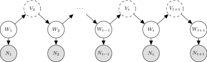
Figure 1: Directed acyclic graph of the shot noise M-ARG(1) in Definition 2.3. White solid circles represent latent gamma random measures, white dashed circles are auxiliary Poisson random measures and grey circles represent the observable Poisson point process.

We now introduce a dynamic version of the Poisson-gamma random field model of Wolpert and Ickstadt, (1998), where the latent intensity is assumed to evolve over time according to a M-ARG(1) process, as in eq. (5).

Definition 2.3.

A shot noise measure-valued auto-regressive gamma process of order 1, or $\textnormal{SN-M-ARG}(1)$, is the time-varying shot noise process defined as

$$N_{t}\mid W_{t}\sim\textnormal{PP}(N_{t}\mid\Lambda_{t})$$

where $(W_{t})_{t\geq 1}$ is a M-ARG(1) process of parameters $(\beta_{t},c_{t})_{t\geq 2}$, $\Lambda_{t}(\mathrm{d}y)=\kappa_{t}\lambda_{t}(y)\ell(\mathrm{d}y)$ is the random intensity measure, $\lambda_{t}(y)=\int_{\Theta}K_{\phi}(y,\theta)W_{t}(\mathrm{d}\theta)$ its density, $\ell(\mathrm{d}y)$ is a $\sigma$-finite measure on $\mathbb{Y}$, $K_{\phi}$ is a positive density kernel on $\mathbb{Y}\times\Theta$, and $(\kappa_{t})_{t\geq 1}$ a deterministic process.

The directed acyclic graph of the SN-M-ARG(1) is given in Fig. 1. The sequence of coefficients $(\kappa_{t})_{t\geq 1}$ captures temporal variations by including covariates and deterministic components, such as seasonality, cycle, and trend. The measure $\ell(dy)$ identifies the deterministic spatial component and may include covariates. Finally, the process $(W_{t})_{t\geq 1}$ incorporates temporal and spatial unobservable factors. This makes the model well-suited for the statistical modelling of spatiotemporal data. The intensity $\Lambda_{t}$ is related to the family of multiplicative intensities that can be written in the general form

$$\Lambda_{t}(\mathrm{d}y)=\tilde{\lambda}_{1}(t)\tilde{\lambda}_{2}(y)S(y,t)\mathrm{d}y,$$

where $S(y,t)$ is a spatiotemporal residual process and $\tilde{\lambda}_{i}$ ($i=1,2$) are deterministic components. In our construction $\tilde{\lambda}_{1}(t)=\kappa_{t}$, $\tilde{\lambda}_{2}(y)\mathrm{d}y=\ell(\mathrm{d}y)$, and the residual process $S(y,t)=\int_{\Theta}K_{\phi}(y,\theta)W_{t}(\mathrm{d}\theta)$ has a simple autoregressive structure well-suited for sequential prediction. This structure guarantees analytical tractability and allows for non-stationarity of the residual process and observed counts.

For $N_{t}$ to be well-defined, one needs some integrability conditions. We already assumed that $H$ is a locally finite measure. We shall assume that $\bar{W}_{1}(\cdot)=\textnormal{E}(W_{1}(\cdot))$ is also locally finite and that for every bounded measurable $B\subset\mathbb{Y}$ it holds:

$$\int_{B}K_{\phi}(y,\theta)\ell(\mathrm{d}y)<+\infty\;\;\forall\theta,\quad\int_{B}\int_{\Theta}K_{\phi}(y,\theta)\>[H(\mathrm{d}\theta)+\bar{W}_{1}(\mathrm{d}\theta)]\ell(\mathrm{d}y)<+\infty.$$ (7)

Proposition 2.3.

If eq. (7) holds, then $(N_{t})_{t\geq 1}$ is a locally finite counting process.

Remark 2.

A simulation method for $(N_{t})_{t\geq 1}$ can be derived by extending the inverse Lévy measure algorithm of Wolpert and Ickstadt, (1998). This truncation-based approach generates samples from the exact target distribution without any approximation error other than the unavoidable truncation error and converges in distribution as the truncation level increases.

3 Limit distributions, moments, covariances

3.1 Conditional Laplace functionals and mean for $(W_{t})_{t\geq 1}$

The conditional Laplace functional of a $\textnormal{M-ARG}(1)$ process at any lag $h\geq 1$ has the appealing feature of being linear in $W_{t}$. For ease of notation, for every $t\geq 1$ and $h\geq 1$ let $\rho_{t+1}\coloneqq\beta_{t+1}c_{t+1}$ and define

$$\rho_{t+h|t}\coloneqq\prod_{j=t+1}^{t+h}\rho_{j},\quad c_{t+h|t}\coloneqq c_{t+h}+\sum_{j=t+1}^{t+h-1}c_{j}\Big{(}\prod_{i=j+1}^{t+h}\rho_{i}\Big{)},\quad\beta_{t+h|t}\coloneqq\rho_{t+h|t}c_{t+h|t}^{-1},$$ (8)

where we use the convention $c_{t+1|t}=c_{t+1}$. Finally, if $(M,N)$ is a vector of random measures, write $\mathcal{L}_{M\mid N}(f)\coloneqq\textnormal{E}\big{(}e^{-\int f\>\mathrm{d}M}\mid N\big{)}$ for the conditional Laplace functional.

Proposition 3.1.

For any $f\in\textnormal{BM}_{+}(\Theta)$, $t\geq 1$ and $h\geq 1$

$$\mathcal{L}_{W_{t+h}\mid W_{t}}(f)=\exp\Big{(}-\!\!\int_{\Theta}\log(1+c_{t+h|t}f(\theta))\>H(\mathrm{d}\theta)-\!\int_{\Theta}\dfrac{\rho_{t+h|t}f(\theta)}{1+c_{t+h|t}f(\theta)}\>W_{t}(\mathrm{d}\theta)\Big{)}.$$

Therefore, the conditional law of $W_{t+h}$ given $W_{t}$ is the same as a $\textnormal{Nc}\mathcal{G}a\textnormal{P}\big{(}H,\beta_{t+h|t}W_{t},c_{t+h|t}^{-1}\big{)}$.

As a corollary of the previous proposition, one can compute the conditional mean measure at any lag $h\geq 1$, which turns out to be linear in the past realisations of the process.

Corollary 1 (Conditional mean measures).

For $t\geq 1$, $h\geq 1$ and any measurable set $A\subset\Theta$

$$\textnormal{E}\big{(}W_{t+h}(A)\mid W_{t}\big{)}=c_{t+h|t}H(A)+\rho_{t+h|t}W_{t}(A).$$

3.2 Stationary distributions

Provided that the coefficients of the M-ARG(1) process do not depend on $t$ and satisfy a suitable condition, the process admits a gamma limiting distribution and a stationary version in the gamma process family.

Proposition 3.2 (Stationary and limiting for $(W_{t})_{t}$).

If $c_{t+1}=c$ and $\beta_{t+1}=\beta$ for all $t\geq 1$ and $\rho=\beta c<1$, then

$$\lim_{h\to+\infty}\mathcal{L}_{W_{t+h}\mid W_{t}}(f)=\exp\Big{(}-\!\!\int_{\Theta}\log\Big{(}1+\dfrac{c}{1-\rho}f(\theta)\Big{)}\>H(\mathrm{d}\theta)\Big{)},\quad f\in\textnormal{BM}_{+}(\Theta).$$

Moreover, the limiting distribution is also invariant, that is, if $W_{t}\sim\mathcal{G}a\textnormal{P}\big{(}W_{t}\mid H,(1-\rho)/c\big{)}$ then $W_{t+h}\sim\mathcal{G}a\textnormal{P}\big{(}W_{t+h}\mid H,(1-\rho)/c\big{)}$, for every $h\geq 1$.

Similarly, one obtains a limiting process and a stationary distribution for the shot noise process $(N_{t})_{t\geq 1}$, which is a Poisson-gamma random field (Wolpert and Ickstadt,, 1998).

Proposition 3.3 (Stationary and limiting for $(N_{t})_{t}$).

Assume eq. (7) holds. Let $c_{t+1}=c$, $\beta_{t+1}=\beta$, $\kappa_{t}=1$ for all $t\geq 1$ and $\rho=\beta c<1$. Then the limiting law of $(N_{t})_{t\geq 1}$ is the one of a Poisson-gamma random field defined in eq. (6), with $(1-\rho)/c$ in place of $c$. Equivalently, for every $f$ in $\textnormal{BM}_{+}(\mathbb{Y})$ one has $\lim_{t\to+\infty}\mathcal{L}_{N_{t}}(f)=\mathcal{L}_{N_{\infty}}(f)$, where

$$\mathcal{L}_{N_{\infty}}(f)=\exp\Big{(}-\!\!\int_{\Theta}\log\Big{(}1+\dfrac{c}{1-\rho}\int_{\mathbb{Y}}\big{(}1-e^{-f(y)}\big{)}K_{\phi}(y,\theta)\>\ell(\mathrm{d}y)\Big{)}\>H(\mathrm{d}\theta)\Big{)}.$$

Moreover, if $W_{1}\sim\mathcal{G}a\textnormal{P}(W_{1}\mid H,(1-\rho)/c)$, then the process $(N_{t})_{t\geq 1}$ is stationary in the sense that $N_{t}\stackrel{{\scriptstyle\mathscr{L}}}{{=}}N_{\infty}$ for every $t$, where $N_{\infty}$ has Laplace functional $\mathcal{L}_{N_{\infty}}$.

3.3 Moments and Covariances

We now study first- and second-order moment measures (both in space and time) of the M-ARG(1) and SN-M-ARG(1) $(W_{t})_{t\geq 1}$ and $(N_{t})_{t\geq 1}$, respectively, by exploiting the properties of completely random measures and the results in Proposition 1.

Proposition 3.4 (Moments of $(W_{t})_{t}$).

Let $g_{1},g_{2}$ be measurable functions on $\Theta$. Define $\bar{W}_{1}(\cdot)\coloneqq\textnormal{E}(W_{1}(\cdot))$ and $W_{t}(g_{i})=\int_{\Theta}g_{i}(\theta)W_{t}(\mathrm{d}\theta)$, with $i=1,2$. Then for $t\geq 1$

$$\textnormal{E}(W_{t}(g_{1}))=c_{t|1}\int_{\Theta}g_{1}(\theta)H(\mathrm{d}\theta)+\rho_{t|1}\int_{\Theta}g_{1}(\theta)\bar{W}_{1}(\mathrm{d}\theta),$$ (9)

$$\begin{split}\textnormal{cov}(W_{t}(g_{1}),W_{t}(g_{2}))&=c_{t|1}^{2}\int_{\Theta}g_{1}(\theta)g_{2}(\theta)H(\mathrm{d}\theta)+2\rho_{t|1}c_{t|1}\int_{\Theta}g_{1}(\theta)g_{2}(\theta)\bar{W}_{1}(\mathrm{d}\theta)\\ &\quad+\rho_{t|1}^{2}\textnormal{cov}(W_{1}(g_{1}),W_{1}(g_{2})),\end{split}$$ (10)

provided the integrals on the right-hand side are well-defined, and

$$\textnormal{cov}(W_{t}(g_{1}),W_{t+h}(g_{2}))=\rho_{t+h|t}\textnormal{cov}(W_{t}(g_{1}),W_{t}(g_{2})),$$ (11)

where $c_{t|1}$, $\rho_{t|1}$ and $\rho_{t+h|t}$ are defined in eq. (8) with the convention $c_{1|1}=0$ and $\rho_{1|1}=1$.

Remark 3.

As a special case of Proposition 3.4, taking $g_{1}(\theta)=\mathds{1}\{\theta\in A_{1}\}$ and $g_{2}(\theta)=\mathds{1}\{\theta\in A_{2}\}$, one obtains expressions for $\textnormal{cov}(W_{t}(A_{1}),W_{t+h}(A_{2}))$ with $h\geq 0$. Under the assumptions of Proposition 3.2, when the process is time stationary, then $W_{t}\sim\mathcal{G}a\textnormal{P}\big{(}W_{t}\mid H,(1-\rho)/c\big{)}$, $\rho_{t+h|t}=\rho^{h}$, $W_{t}(A)\sim\mathcal{G}a(H(A),(1-\rho)/c)$ and from eq. (11) it follows

$$\textnormal{cov}(W_{t}(A),W_{t+h}(A))=\rho^{h}\textnormal{cov}(W_{t}(A),W_{t}(A))=\rho^{h}\textnormal{var}(W_{t}(A))=\rho^{h}H(A)\frac{c^{2}}{(1-\rho)^{2}}.$$

In particular, for any measurable $A\subseteq\Theta$, $\textnormal{corr}(W_{t}(A),W_{t+h}(A))=\rho^{h}$.

Following Definitions 4.2, 4.3, and 4.8 in Møller and Waagepetersen, (2003), the first- and second-order moment statistics of $(N_{t})_{t\geq 1}$ can be derived from the intensity $\mathfrak{D}^{(1)}_{t}(y)$, the second-order product density $\mathfrak{D}_{t}^{(2)}(y_{1},y_{2})$ and the cross second-order pair intensity $\mathfrak{D}^{(2)}_{t,t+h}(y_{1},y_{2})$, which are positive functions such that for bounded measurable $B_{1},B_{2}\subset\mathbb{Y}$:

$$\begin{split}\textnormal{E}(N_{t}(B_{1}))&=\int_{B_{1}}\mathfrak{D}^{(1)}_{t}(y)\ell(\mathrm{d}y),\\ \textnormal{E}(N_{t}(B_{1})N_{t}(B_{2}))&=\int_{B_{1}\cap B_{2}}\!\!\mathfrak{D}^{(1)}_{t}(y)\ell(\mathrm{d}y)+\int_{B_{1}\times B_{2}}\!\!\mathfrak{D}_{t}^{(2)}(y_{1},y_{2})\ell(\mathrm{d}y_{1})\ell(\mathrm{d}y_{2}),\\ \textnormal{E}(N_{t}(B_{1})N_{t+h}(B_{2}))&=\int_{B_{1}\times B_{2}}\!\!\mathfrak{D}_{t,t+h}^{(2)}(y_{1},y_{2})\ell(\mathrm{d}y_{1})\ell(\mathrm{d}y_{2}).\end{split}$$ (12)

In our shot noise process, conditionally on $(W_{t},W_{t+h})$, $(N_{t},N_{t+h})$ are independent Poisson random measures with random mean measures $\Lambda_{t}(\mathrm{d}y)=\kappa_{t}\lambda_{t}(y)\ell(\mathrm{d}y)$ and $\Lambda_{t+h}(\mathrm{d}y)=\kappa_{t+h}\lambda_{t+h}(y)\ell(\mathrm{d}y)$, respectively, where $\lambda_{t}(y)$ is given in Definition 2.3. Combining this observation with the fact that $\textnormal{E}(N(B_{1}))=\Lambda(B_{1})$ and $\textnormal{E}(N(B_{1})N(B_{2}))=\Lambda(B_{1}\cap B_{2})+\Lambda(B_{1})\Lambda(B_{2})$, for $N\sim\textnormal{PP}(N\mid\Lambda)$ (Last and Penrose,, 2018, eq. 4.26), it follows:

$$\begin{split}&\mathfrak{D}^{(1)}_{t}(y)=\kappa_{t}\textnormal{E}(\lambda_{t}(y)),\qquad\mathfrak{D}_{t}^{(2)}(y_{1},y_{2})=\kappa_{t}^{2}\textnormal{E}(\lambda_{t}(y_{1})\lambda_{t}(y_{2})),\\ &\mathfrak{D}^{(2)}_{t,t+h}(y_{1},y_{2})=\kappa_{t}\kappa_{t+h}\textnormal{E}(\lambda_{t}(y_{1})\lambda_{t+h}(y_{2})).\end{split}$$ (13)

For dependent sequences of shot noise processes, it is usually difficult to find tractable expressions for the intensity $\mathfrak{D}^{(1)}$ and the correlation densities $\mathfrak{D}^{(2)}_{t}$ and $\mathfrak{D}^{(2)}_{t,t+h}$ (see Jalilian et al.,, 2015, for further discussion). Instead, such expressions are available for our SN-M-ARG model.

The following integrability conditions are needed to guarantee the convergence of the integrals appearing on the right-hand side of eq. (12).

1. For every bounded measurable $B\subset\mathbb{Y}$ condition (7) is satisfied.

2. For every couple of bounded measurable sets $B_{1},B_{2}\subset\mathbb{Y}$ it holds:

   $$\int_{B_{1}\times B_{2}}\int_{\Theta}K_{\phi}(y_{1},\theta)K_{\phi}(y_{2},\theta)\>[H(\mathrm{d}\theta)+\bar{W}_{1}(\mathrm{d}\theta)]\ell(\mathrm{d}y_{1})\ell(\mathrm{d}y_{2})<+\infty.$$

3. For every couple of bounded measurable sets $B_{1},B_{2}\subset\mathbb{Y}$ it holds:

   $$\textnormal{E}\Big{(}\int_{B_{1}\times B_{2}}\int_{\Theta}K_{\phi}(y_{1},\theta_{1})W_{1}(\mathrm{d}\theta_{2})\int_{\Theta}K_{\phi}(y_{2},\theta_{2})W_{1}(\mathrm{d}\theta_{2})\ell(\mathrm{d}y_{1})\ell(\mathrm{d}y_{2})\Big{)}<+\infty.$$

Conditions $(H_{1})$-$(H_{3})$ are always satisfied when the kernel $K_{\phi}$ is bounded, and the expected initial measure $\bar{W}_{1}$ and the base measure $H$ are locally bounded.

Simpler forms for eq. (13) can be deduced in the time-stationary regime guaranteed by Proposition 3.3 when the following stationarity condition is satisfied:

1. for all $t\geq 1$ $c_{t}=c$, $\beta_{t}=\beta$, $\rho=\beta c<1$ and $W_{1}\sim\mathcal{G}a\textnormal{P}(W_{1}\mid H,(1-\rho)/c)$.

Proposition 3.5 (First and second order statistics of $(N_{t})_{t}$).

Let $(N_{t})_{t\geq 1}$ be a $\textnormal{SN-M-ARG}(1)$. Assume $(H_{1})$-$(H_{3})$. Then, for every $y$, $y_{1}$ and $y_{2}$ in $\mathbb{Y}$ and for every $t$ and $h$ strictly positive integers it holds:

$$\mathfrak{D}^{(1)}_{t}(y)=\kappa_{t}c_{t|1}\int_{\Theta}K_{\phi}(y,\theta)H(\mathrm{d}\theta)+\kappa_{t}\rho_{t|1}\int_{\Theta}K_{\phi}(y,\theta)\bar{W}_{1}(\mathrm{d}\theta),$$

$$\mathfrak{D}^{(2)}_{t,t+h}(y_{1},y_{2})=\kappa_{t+h}\rho_{t+h|t}{\kappa_{t}}\mathfrak{D}^{(2)}_{t}(y_{1},y_{2})+\mathfrak{D}^{(1)}_{t}(y_{1})\kappa_{t+h}c_{t+h|t}\int_{\Theta}K_{\phi}(y_{2},\theta)H(\mathrm{d}\theta)$$

$$\begin{split}\mathfrak{D}^{(2)}_{t}(y_{1},y_{2})&=\mathfrak{D}^{(1)}_{t}(y_{1})\mathfrak{D}^{(1)}_{t}(y_{2})+\kappa_{t}^{2}c_{t|1}^{2}\int_{\Theta}K_{\phi}(y_{1},\theta)K_{\phi}(y_{2},\theta)H(\mathrm{d}\theta)\\ &\quad+\kappa_{t}^{2}\rho_{t|1}^{2}\textnormal{cov}\Big{(}\int_{\Theta}K_{\phi}(y_{1},\theta)W_{1}(\mathrm{d}\theta),\int_{\Theta}K_{\phi}(y_{2},\theta)W_{1}(\mathrm{d}\theta)\Big{)}.\end{split}$$ (14)

The previous proposition can be extended to $h=0$, by using the convention $c_{t|t}=0$ and $\rho_{t|t}=1$, so that $\mathfrak{D}^{(2)}_{t,t}(y_{1},y_{2})=\mathfrak{D}^{(2)}_{t}(y_{1},y_{2})$. Expressions of the first and second-order statistics simplify under the stationarity assumption $(H_{4})$, as stated below.

Proposition 3.6 (First and second order statistics of stationary $(N_{t})_{t}$).

Let $(N_{t})_{t\geq 1}$ be a $\textnormal{SN-M-ARG}(1)$, assume integrability $(H_{1})$-$(H_{3})$ and time stationarity $(H_{4})$. Then for every $y$, $y_{1}$, and $y_{2}$ in $\mathbb{Y}$ and $t$ positive integers,

$$\mathfrak{D}^{(1)}_{t}(y)=\frac{c\kappa_{t}}{1-\rho}\int_{\Theta}K_{\phi}(y,\theta)H(\mathrm{d}\theta)$$ (15)

$$\mathfrak{D}^{(2)}_{t}(y_{1},y_{2})-\mathfrak{D}^{(1)}_{t}(y_{1})\mathfrak{D}^{(1)}_{t}(y_{2})=\frac{c^{2}\kappa_{t}^{2}}{(1-\rho)^{2}}\int_{\Theta}K_{\phi}(y_{1},\theta)K_{\phi}(y_{2},\theta)H(\mathrm{d}\theta).$$ (16)

The so-called cross-pair correlation function (see Møller and Waagepetersen,, 2003, def. 4.8) of the point process $(N_{t})_{t\geq 1}$ is

$$\mathscr{R}_{t_{1},t_{2}}(y_{1},y_{2})\coloneqq\frac{\mathfrak{D}^{(2)}_{t_{1},t_{2}}(y_{1},y_{2})}{\mathfrak{D}^{(1)}_{t_{1}}(y_{1})\mathfrak{D}^{(1)}_{t_{2}}(y_{2})}=\frac{\textnormal{E}(\lambda_{t_{1}}(y_{1})\lambda_{t_{2}}(y_{2}))}{\textnormal{E}(\lambda_{t_{1}}(y_{1}))\textnormal{E}(\lambda_{t_{2}}(y_{2}))},$$

where the second equality follows by eq. (13). The general expression of $\mathscr{R}$ for our SN-M-ARG can be easily deduced using Proposition 3.5. In the time-stationary regime of Proposition 3.6, one has

$$\mathscr{R}_{t,t+h}(y_{1},y_{2})=\rho^{h}\frac{\int_{\Theta}K_{\phi}(y_{1},\theta)K_{\phi}(y_{2},\theta)H(\mathrm{d}\theta)}{\int_{\Theta}K_{\phi}(y_{1},\theta_{1})H(\mathrm{d}\theta_{1})\int_{\Theta}K_{\phi}(y_{2},\theta_{2})H(\mathrm{d}\theta_{2})}+1$$

for $t\geq 1$ and $h\geq 0$. Indeed, in this case $\rho_{t+h|t}=\rho^{h}$ and $c_{t+h|t}=c(1-\rho^{h})/(1-\rho)$, so that combining eq. (3.5), (15), and (16) the previous expression follows easily.

In the time-stationary case with $\kappa_{t}=1$ for every $t$, since $\mathscr{R}_{t,t+h}\geq 1$, the process is attractive. Intuitively, pairs of points are more likely to occur at locations $y_{1}$ and $y_{2}$ than for a Poisson process (see, e.g. Møller and Waagepetersen,, 2003). Besides, the attraction effect decreases at larger temporal lags $h$. In this case, the cross pair correlation function $\mathscr{R}_{t_{1},t_{2}}$ is time-homogeneous since it depends on $h=|t_{1}-t_{2}|$, but it can be either homogeneous or non-homogeneous in space following the choice of $K_{\phi}$ and $H$. For example, if $\mathbb{Y}=\Theta=\mathds{R}^{d}$, $H$ and $\ell(\mathrm{d}y)$ are the Lebesgue measure on $\mathds{R}^{d}$ and $K_{\phi}(\theta,y)=(\pi\phi^{2})^{-d/2}\exp\{-\phi^{-2}\|\theta-y\|^{2}\}$ is a Gaussian kernel, then $\mathscr{R}_{t,t+h}(y_{1},y_{2})=C_{1}\rho^{|h|}e^{-C_{2}\|y_{1}-y_{2}\|^{2}}+1$, $C_{1}=(2\pi\phi^{2})^{-d/2}$, and $C_{2}=(2\phi^{2})^{-1}$.

Combining Propositions 3.5 and 3.6 with eq. (12), one obtains closed-form expressions of the second-order moments of $N_{t}$, given in the next two Corollaries. For simplicity, set $K_{\phi}(A,\theta)=\int_{A}K_{\phi}(y,\theta)\ell(\mathrm{d}y)$.

Corollary 2.

Assume $(H_{1})$-$(H_{3})$, then for measurable sets $B_{1},B_{2}\subset\Theta$ and integers $t\geq 1$ and $h\geq 0$, it holds

$$\begin{split}\textnormal{cov}(&N_{t}(B_{1}),N_{t+h}(B_{2}))=\kappa_{t}\kappa_{t+h}\rho_{t+h|t}c_{t|1}^{2}\int_{\Theta}K_{\phi}(B_{1},\theta)K_{\phi}(B_{2},\theta)(H(\mathrm{d}\theta)+2\beta_{t|1}\bar{W}_{1}(\mathrm{d}\theta))\\ &+\kappa_{t}\kappa_{t+h}\rho_{t+h|t}\rho_{t|1}^{2}\textnormal{cov}\Big{(}\int_{\Theta}K_{\phi}(B_{1},\theta)W_{1}(\mathrm{d}\theta),\int_{\Theta}K_{\phi}(B_{2},\theta)W_{1}(\mathrm{d}\theta)\Big{)}\\ &+\kappa_{t}\mathds{1}\{h=0\}\int_{\Theta}c_{t|1}K_{\phi}(B_{1}\cap B_{2},\theta)\big{(}H(\mathrm{d}\theta)+\beta_{t|1}\bar{W}_{1}(\mathrm{d}\theta)\big{)},\end{split}$$

provided all the quantities on the right-hand side are well-defined.

Corollary 3.

Assume integrability $(H_{1})$-$(H_{3})$ and time stationarity $(H_{4})$, then

$$\begin{split}\textnormal{E}(N_{t}(B_{1}))&=\frac{c\kappa_{t}}{1-\rho}\int_{\Theta}K_{\phi}(B_{1})\>H(\mathrm{d}\theta),\\ \textnormal{cov}(N_{t}(B_{1}),N_{t+h}(B_{2}))&=\mathds{1}\{h=0\}\frac{c\kappa_{t}}{1-\rho}\int_{\Theta}K_{\phi}(B_{1}\cap B_{2},\theta)\>H(\mathrm{d}\theta)\\ &\quad+\frac{\rho^{h}c^{2}\kappa_{t}\kappa_{t+h}}{(1-\rho)^{2}}\int_{\Theta}K_{\phi}(B_{1},\theta)K_{\phi}(B_{2},\theta)\>H(\mathrm{d}\theta),\end{split}$$

provided all the quantities on the right are well-defined.

We remark that, in the time-stationary case, the expression of $\textnormal{cov}(N_{t}(B_{1}),N_{t}(B_{2}))$ for each fixed $t=1,\ldots,T$, coincides with the result given in Wolpert and Ickstadt, (1998) for the Poisson-gamma random field.

Using arguments similar to those used to obtain first and second-order statistics, one can deduce closed-form expressions for high-order moments. For simplicity, we provide the high-order moments only in the time-stationary case.

Proposition 3.7.

Assume time stationarity $(H_{4})$ and

$$J_{r}(B)\coloneqq\frac{\gamma(r)c^{r}}{(1-\rho)^{r}}\int K_{\phi}(B,\theta)^{r}\>H(\mathrm{d}\theta)<+\infty,$$

for $r=1,\dots,m$, then

$$\textnormal{E}(N_{t}(B)^{m})=\sum_{j=1}^{m}S_{m,j}\,\,\kappa_{t}^{j}\!\!\sum_{\begin{subarray}{c}\ell_{1},\dots,\ell_{j}\geq 0\\ \sum_{r=1}^{j}r\ell_{r}=j\end{subarray}}c(\ell_{1},\dots,\ell_{j})\prod_{r=1}^{j}J_{r}(B)^{\ell_{r}}$$ (17)

where $c(\ell_{1},\dots,\ell_{j})=j!\big{(}\prod_{r=1}^{j}(r!)^{\ell_{r}}\ell_{r}!\big{)}^{-1}$ and $S_{m,j}$ are Stirling numbers of second kind.

4 Bayesian inference

4.1 Data augmentation

Given $\Lambda_{t}$, $N_{t+1}$ is an integer-valued measure which can be represented as the collection of a random number $N_{t}^{y}\sim\mathcal{P}oi(N_{t}^{y}\mid\Lambda_{t}(\mathbb{Y}))$ of unit point masses at not-necessarily-distinct points $y_{i,t}$. In the real-data illustration, $N_{t}^{y}$ is the total number of observed event points (fires) at the time (month) $t$. The points $y_{i,t}$ are drawn conditionally independently from

$$y_{i,t}\mid W_{t},N_{t}^{y}\stackrel{{\scriptstyle iid}}{{\sim}}Q_{t}^{y},\qquad i=1,\ldots,N_{t}^{y},$$

where $Q_{t}^{y}$ is the random probability measure resulting from the mixture

$$Q_{t}^{y}(\mathrm{d}y) =\frac{\Lambda_{t}(\mathrm{d}y)}{\Lambda_{t}(\mathbb{Y})}=\sum_{j=1}^{\infty}w_{j,t}^{*}K_{\phi}(y,\theta_{j,t})\ell(\mathrm{d}y),$$ (18)

where $w_{j,t}^{*}=w_{j,t}/\Lambda_{t}(\mathbb{Y})$, for $j=1,2,\ldots$, are normalised weights. Following Wolpert and Ickstadt, (1998), we consider the data augmentation approach and introduce a collection of latent allocation variables for resolving the mixture. As a result, one obtains a random measure $Z_{t+1}$ on $\mathbb{Y}\times\Theta$ such that

$$Z_{t+1}\mid W_{t},V_{t+1},W_{t+1} \sim\textnormal{PP}\big{(}Z_{t+1}\mid\kappa_{t+1}K_{\phi}(y,\theta)\ell(\mathrm{d}y)W_{t+1}(\mathrm{d}\theta)\big{)}$$

$$N_{t+1}(\mathrm{d}y) =Z_{t+1}(\mathrm{d}y\times\Theta).$$

The random measure $Z_{t+1}$ assigns unit mass to each pair $(y_{i,t+1},\theta_{i,t+1}^{*})$, where $\theta_{i,t+1}^{*}\in\Theta$ is the atom of the latent measure $W_{t+1}$ to which the observation $y_{i,t+1}$ has been allocated.

4.2 Model specification

In the application, we assume that both $\Theta$ and $\mathbb{Y}$ are bounded sets in $\mathds{R}^{2}$ and that the kernel is a two-dimensional normal density with covariance matrix $\phi^{2}\textnormal{I}_{2}$, that is $K_{\phi}(y,\theta)=\mathcal{N}_{2}(y\mid\theta,\phi^{2}\textnormal{I}_{2})$. As for the deterministic component $\kappa_{t}$, we assume $\kappa_{t}=\exp(\eta^{{\mathrm{\scriptscriptstyle T}}}x_{t})$ where $\eta$ is a parameter vector and the $x_{t}\in\mathds{R}^{m}$ are time-dependent covariates. See Section 5 for an illustration.

To reduce the complexity of the parameter space, we choose a discrete base measure $H$ with support $\Theta^{g}=\{\theta_{1},\ldots,\theta_{N^{g}}\}$, that is $H(\mathrm{d}\theta)=\sum_{j=1}^{N^{g}}\alpha_{j}\delta_{\theta_{j}}(\mathrm{d}\theta)$. This can be considered as a discretisation of a continuous measure $H(\mathrm{d}\theta)=h(\theta)\mathrm{d}\theta$, with $\alpha_{j}$ the value of $H(A_{j})$, $(A_{j})_{j=1,\dots,N^{g}}$ a suitable tessellation of $\Theta$, and $\theta_{j}$ the “centre” of the cell $A_{j}$. In this way $H$ is parametrised by a $N^{g}$-dimensional vector $(\alpha_{1},\dots,\alpha_{N^{g}})$.

With this choice, the measure-valued noncentral gamma process $(W_{t})_{t\geq 1}$ evaluated at $\Theta^{g}$ results in a collection of scalar noncentral gamma processes. In particular, for each $j=1,\ldots,N^{g}$, define $w_{j,t}\coloneqq W_{t}(\{\theta_{j}\})$ to obtain:

$$w_{j,t}\mid w_{j,t-1}\sim\textnormal{Nc}\mathcal{G}a(w_{j,t}\mid\alpha_{j},\beta w_{j,t-1},c_{t}^{-1}).$$ (19)

We can describe $Z_{t}$ with the collection of the data points $y_{i,t}$ and a set of allocation variables $z_{i,t}$, such that $\theta_{i,t}^{*}=\theta_{z_{i,t}}\in\Theta^{g}$ is the point in $\Theta^{g}$ which the observation $y_{i,t}$ has been allocated to. Therefore, we obtain $N_{t}^{y}\sim\mathcal{P}oi(N_{t}^{y}\mid\Lambda_{t}(\mathbb{Y}))$ and

$$(y_{i,t},z_{i,t})\mid N_{t}^{y}\stackrel{{\scriptstyle iid}}{{\sim}}\kappa_{t}\sum_{j=1}^{N^{g}}\frac{w_{j,t}}{\Lambda_{t}(\mathbb{Y})}K_{\phi}(y,\theta_{z_{j,t}})\delta_{\theta_{z_{j,t}}}(\mathrm{d}\theta)\ell(\mathrm{d}y),\quad i=1,\dots,N_{t}^{y}.$$ (20)

4.3 Bayesian inference

The collection of unknown parameters is the vector $\bm{\psi}=\{\bm{\alpha},\beta,\mathbf{c},\phi,r,\eta\}$, with $\bm{\alpha}=\{\alpha_{1},\ldots,\alpha_{N^{g}}\}$ and $\mathbf{c}=\{c_{1},\ldots,c_{T}\}$, for which a prior need to be specified. We assume the following prior for the static parameters:

$$\alpha_{j}\mid\gamma \mathbin{\overset{iid}{\kern 0.0pt\sim}}\mathcal{G}a(\alpha_{j}\mid\underline{a}_{\alpha},\gamma\underline{b}_{\alpha}),\;\;j=1,\ldots,N^{g},\qquad\beta\mid\gamma\sim\mathcal{G}a(\beta\mid\underline{a}_{\beta},\gamma\underline{b}_{\beta}),$$

$$\gamma \sim\mathcal{G}a(\gamma\mid\underline{a}_{\gamma},\underline{b}_{\gamma}),\qquad\phi\sim\mathcal{G}a(\phi\mid\underline{a}_{\phi},\underline{b}_{\phi}).$$

We consider two alternative specifications for the scale parameter $\mathbf{c}$: i) constant, that is, $c_{t}=c$ for every $t$; ii) time-varying. In the first setting, we assume $c\sim\mathcal{G}a(c\mid\underline{a}_{c},\underline{b}_{c})$, whereas in the second one, we assume the hierarchical prior distribution:

$$c_{t}\mid r \mathbin{\overset{iid}{\kern 0.0pt\sim}}\mathcal{G}a(c_{t}\mid r^{2}/\underline{\sigma}^{2}_{c},r/\underline{\sigma}^{2}_{c}),\;\;t=1,\ldots,T,\qquad r\sim\mathcal{G}a(r\mid\underline{a}_{r},\underline{b}_{r}),$$

such that $\textnormal{E}(c_{t}\mid r)=r$. Finally, a multivariate Gaussian prior is assumed for the coefficient vector, $\eta\sim\mathcal{N}_{m}(\eta\mid\underline{\bm{\mu}}_{\eta},\underline{\Sigma}_{\eta})$.

Let $\mathbf{y}_{1:T}=\{y_{1},\ldots,y_{T}\}$, $\mathbf{w}_{1:T}=\{w_{1},\ldots,w_{T}\}$ and $\mathbf{z}_{1:T}=\{z_{1},\ldots,z_{T}\}$, from eq. (19)-(20), the complete-data likelihood function $L(\mathbf{y}_{1:T},\mathbf{z}_{1:T},\mathbf{w}_{1:T}\mid\bm{\psi})$ is

$$\prod_{t=1}^{T}\mathcal{P}oi(N_{t}^{y}\mid\Lambda_{t}(\mathbb{Y}))\prod_{j=1}^{N^{g}}\textnormal{Nc}\mathcal{G}a(w_{j,t}\mid\alpha_{j},\beta w_{j,t-1},c_{t}^{-1})\prod_{i=1}^{N_{t}^{y}}\frac{w_{z_{i,t},t}\mathcal{N}_{2}(y_{i,t}\mid\theta_{z_{i,t}},\textnormal{I}_{2}\phi^{2})}{\Lambda_{t}(\mathbb{Y})}.$$

The joint posterior of the model parameters $\bm{\psi}$ and the latent variables $\mathbf{w}_{1:T}$ and $\mathbf{z}_{1:T}$ is approximated using a Particle Gibbs sampler (Andrieu et al.,, 2010; Kantas et al.,, 2015). To cope with the high dimensionality of the latent space, we combine a blocking strategy with a conditional Sequential Monte Carlo algorithm (Chopin et al.,, 2013; Gerber and Chopin,, 2015; Singh et al.,, 2017; Goldman and Singh,, 2021). We assume the latent states are grouped into $L$ blocks of size $S_{\ell}$ each, that is $\mathbf{w}_{1:T}=\{\mathbf{w}_{1,1:T},\ldots,\mathbf{w}_{L,1:T}\}$, where $\mathbf{w}_{\ell,1:T}=\{w_{j,t}:j\in S_{\ell},\,t=1,\ldots,T\}$ and $S_{\ell}\subset\{1,\ldots,N^{g}\}$. At each iteration, the algorithm yields an approximation $\widehat{p}(\mathbf{w}_{\ell,1:T}\mid\mathbf{y}_{1:T},\mathbf{z}_{1:T},\mathbf{w}_{-\ell,1:T},\bm{\psi})$ of the distribution $p(\mathbf{w}_{\ell,1:T}\mid\mathbf{y}_{1:T},\mathbf{z}_{1:T},\mathbf{w}_{-\ell,1:T},\bm{\psi})$. With this approximation at hand, the Particle Gibbs sampler cycles over the following steps:

1. Sample the parameters $\bm{\psi}$ given $\mathbf{y}_{1:T},\mathbf{z}_{1:T}$, and $\mathbf{w}_{1:T}$.

2. Sample the allocation variables $\mathbf{z}_{1:T}$ given $\mathbf{y}_{1:T},\mathbf{w}_{1:T}$, and $\bm{\psi}$.

3. Sample the latent states $\mathbf{w}_{\ell,1:T}$, sequentially for $\ell=1,\ldots,L$, by running a conditional Sequential Monte Carlo algorithm with target $p(\mathbf{w}_{\ell,1:T}\mid\mathbf{y}_{1:T},\mathbf{z}_{1:T},\mathbf{w}_{-\ell,1:T},\bm{\psi})$, and sampling $\mathbf{w}_{\ell,1:T}\sim\widehat{p}(\mathbf{w}_{\ell,1:T}\mid\mathbf{y}_{1:T},\mathbf{z}_{1:T},\mathbf{w}_{-\ell,1:T},\bm{\psi})$.

In Step 1, we draw from the full conditional distribution of the parameters with an adaptive Metropolis-Hastings. The allocation variables in Step 2 are drawn exactly. In Step 3, given the parameters, $\bm{\psi}$, the allocation variables, $\mathbf{z}_{1:T}$, and the other $L-1$ blocks, $\mathbf{w}_{-\ell,1:T}$, the conditional Sequential Monte Carlo for the $\ell$th block $\mathbf{w}_{\ell,1:T}$ is similar to the standard one, but imposes that a prespecified path, $\mathbf{w}_{\ell,1:T}$ with ancestral lineage survives all the resampling steps. The remaining $N-1$ particles are generated as usual. The Supplement provides further details.

5 Illustration

5.1 Data description

Climate change has been a critical factor impacting the risk and extent of wildfires in many areas, such as Australia, California, Canada, Siberia, the Mediterranean coast, and Savannah. Over the past decades, new regions and ecosystems such as tropical forests experienced an increase in the frequency and intensity of large fires with severe impact on ecological systems (e.g., vegetation structure and composition), economy (e.g., loss of properties) and society (e.g., direct and indirect threats to human health and life).

As argued by Balch et al., (2020), the abundance of remote sensed fire data calls for an effort of the science community to investigate changes in the fire regimes and vulnerabilities of society and ecosystems. Measuring the risk and intensity of fires and modelling and predicting their local or global spatiotemporal dynamics can help to support policy decisions in areas affected by future climatic and land-use changes (Hantson et al.,, 2016).

	Constant scale	Time-varying Scale
June $2020$
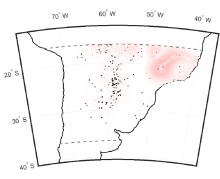
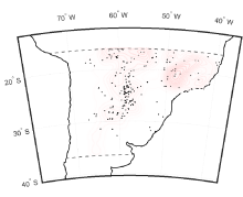
July $2020$
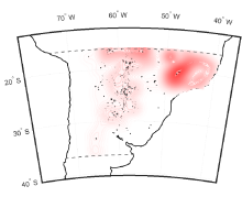
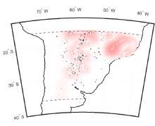
August $2020$
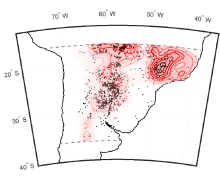
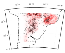
September $2020$

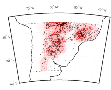
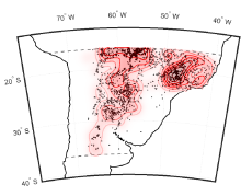
Figure 2: Monthly fires ($\bullet$) between longitude $80^{o}W$ and $40^{o}W$ and latitude $35^{o}S$ and $10^{o}S$ and estimated fire intensity, $\Lambda_{t}(y)$ (shaded areas and contour lines) for models with harmonic components and constant (left) and time-varying (right) scale.

Our application uses satellite observations with high spatiotemporal resolution and broad spatial coverage to study fires in the Amazon forest. Different kinds of satellite data are available to investigate fires. Here, we consider NASA’s Moderate Resolution Imaging Spectroradiometer (MODIS), the first family of remotely sensed fire datasets (Giglio et al.,, 2016). MODIS provides systematic observations of fires over the entire globe and has been used to answer many scientific questions, such as fire dynamics in forests (Csiszar,, 2007) and its impact on air quality and Savannah’s ecosystems.

Fire observations such as fire detection and fire radiative power are collected by MODIS 1-km sensor on Terra and Aqua (see the Supplement for further details). A geographic location, time, and date identify each fire pixel in the dataset. The study area of this paper covers the territory with a longitude between $82^{o}W$ and $34^{o}W$ and a latitude between $40^{o}S$ and $0^{o}$. The area includes the Amazon forest, the world’s largest rainforest, and is central to global warming. The additional pixel-level information allows us to exclude active volcanoes, other static land sources, and offshore fires and select only presumed vegetation fires detected by Terra and Aqua MODIS sensors with detection confidence between 80% and 100%. Figure 2 shows the frequency of observed fires (dots) in Brazil, Bolivia and Peru, which exhibits spatial and temporal patterns.

5.2 Results

We apply our spatiotemporal models with two alternative specifications of the global factor $\kappa_{t}$ proposed in the literature and three different specifications for the scale parameter $c_{t}$. As for $\kappa_{t}$, the first specification (denoted by “$D$”) has a trend and a dry-season dummy variable, that is $\kappa_{t}=\exp(\eta_{0}+\eta_{TR}t+\eta_{D,1}d_{t})$, where $d_{t}$ takes the value one if $t$ is a month of the dry season (from August to December), while the second specification (denoted by “$H$”) has a trend and four harmonic components $\kappa_{t}=\exp(\eta_{0}+\eta_{TR}t+\eta_{S,1}\sin(2\pi\omega_{1}t)+\eta_{C,1}\cos(2\pi\omega_{1}t)+\ldots+\eta_{S,4}\sin(2\pi\omega_{4}t)+\eta_{C,4}\cos(2\pi\omega_{4}t))$. The frequencies have been estimated following the peaks in the spectral density of the time series of the total number of fires. The estimated frequencies $\hat{\omega}_{1}=0.086$, $\hat{\omega}_{2}=0.168$, $\hat{\omega}_{3}=0.254$, and $\hat{\omega}_{4}=0.336$ correspond to annual, semi-annual, four-month and three-month periods, respectively. The three scale parameter specifications are constant scale $c_{t}=c$ for every $t$ (denoted by “$c$”), a time-varying scale $c_{t}$ (indicated by “$v$”) and a monthly specification $c_{t}=c_{t+12}=c_{t+24}\ldots$ for every $t$ (denoted by “$v12$”). We obtain three specifications for the harmonic models denoted by $\mathcal{M}^{H,c}$, $\mathcal{M}^{H,v}$, $\mathcal{M}^{H,v12}$ and three other specifications for the model with seasonal dummies marked by $\mathcal{M}^{D,c}$, $\mathcal{M}^{D,v}$, $\mathcal{M}^{D,v12}$.

Our framework can provide a globally consistent inference of fire trend and seasonality based on high spatial resolution data from a wide region, which is still an open issue in analysing climate-related risks (e.g., see Tyukavina et al.,, 2022). We notice that the Bayesian framework is well-suited for quantifying uncertainty in the model estimate and forecasts, which is currently a crucial issue in evaluating model-based estimates and projections for climate-related variables (Raftery et al.,, 2017).

Model estimates and fitting
	$\mathcal{M}^{H,c}$	$\mathcal{M}^{H,v}$	$\mathcal{M}^{H,v12}$	$\mathcal{M}^{D,c}$	$\mathcal{M}^{D,v}$	$\mathcal{M}^{D,v12}$
(a) Parameter estimates
$\eta_{TR}$	0.040	0.040	0.051	0.035	0.023	0.049
	(0.036,0.053)	(0.038,0.043)	(0.049,0.054)	(0.033,0.040)	(0.022,0.024)	(0.048,0.052)
$\eta_{D,1}$	1.367	1.369	1.984
	(0.947,1.501)	(1.297,1.444)	(1.930,2.038)
$\eta_{S,1}$				-0.155	0.714	0.539
				(-0.218,-0.063)	(0.699,0.733)	(0.528,0.551)
$\eta_{C,1}$				-0.965	-1.028	-1.084
				(-1.010,-0.912)	(-1.052,-1.000)	(-1.109,-1.062)
$\eta_{S,2}$				-0.287	-0.525	-0.594
				(-0.376,-0.181)	(-0.551,-0.498)	(-0.610,-0.576)
$\eta_{C,2}$				0.174	-0.121	0.065
				(0.082,0.236)	(-0.130,-0.110)	(0.051,0.080)
$\eta_{S,3}$				0.173	-0.040	-0.104
				(0.131,0.239)	(-0.058,-0.022)	(-0.114,-0.093)
$\eta_{C,3}$				0.386	0.341	0.307
				(0.355,0.448)	(0.327,0.357)	(0.294,0.320)
$\eta_{S,4}$				0.014	0.157	0.095
				(-0.018,0.060)	(0.131,0.187)	(0.071,0.116)
$\eta_{C,4}$				0.014	0.197	0.074
				(-0.084,0.121)	(0.174,0.215)	(0.064,0.084)
(b) Model fitting (normalised across models)
MSE	0.308	0.103	0.180	0.108	0.090	0.211
MAE	0.201	0.137	0.181	0.152	0.134	0.195
(c) Model forecasting over horizon $h$ (cumulated and normalised across models)
MSE $h=1$	0.1214	0.3111	0.1746	0.0072	0.3111	0.0745
MSE $h=3$	0.0198	0.0752	0.6618	0.0058	0.0752	0.1622
MSE $h=6$	0.0036	0.1611	0.5466	0.0712	0.1612	0.0563
MAE $h=1$	0.1555	0.2490	0.1865	0.0380	0.2490	0.1219
MAE $h=3$	0.0702	0.1501	0.3883	0.0407	0.1501	0.2006
MAE $h=6$	0.0295	0.1848	0.3713	0.1132	0.1849	0.1163

Table 1: Panel (a) reports the posterior mean and $95\%$ posterior credible intervals (in brackets) of the parameters of the global factor $\kappa_{t}$ across models. Panels (b) and (c) show the in- and out-of-sample model diagnostics. For the harmonic ($j=H$) and the dry-season dummy ($j=D$) model the following three specifications are considered: $\mathcal{M}^{j,c}$, constant scale; $\mathcal{M}^{j,v}$ time-varying scale; $\mathcal{M}^{j,v12}$ time-varying scale with monthly seasonal dummy. For model performance, Mean Square Error (MSE) and Mean Absolute Error (MAE) are computed in-sample and normalised across models.

The parameter estimates of the factor $\kappa_{t}$ in Panel (a) of Table 1 and the factor estimates in the second row of Panel (a) and (b) in Fig. 5 in the Supplement provide strong evidence, across specifications, of an exponential trend and seasonal effects for the entire area of interest. The monthly growth rate of the fire intensity varies between 0.023 and 0.051 across models, corresponding to annual percentage growth between 27% and 61%. These findings align with the results reported in other studies on global trends in fire intensity (e.g. Jones et al.,, 2022). There is strong evidence of temporal persistence regarding the dynamic of the latent random measure, which captures the residual local spatiotemporal variability. The estimated persistence parameter in the constant scale specification is $\hat{\rho}=0.471$ and $\hat{\rho}=0.527$ in the dummy and harmonic models, respectively. In the time-varying scale models, $\hat{\rho}_{t}$ takes values between 0.199 and 0.995 depending on the season, with large persistence of fires during January and July and low persistence intensity during November and December.

	Constant scale	Time-varying Scale
June $2020$
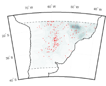
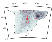
September $2020$

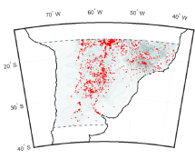
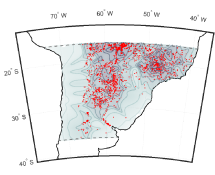
Figure 3: Coefficient of variation of the fire intensity $\Lambda_{t}(y)$ (shaded areas and contour lines) for models with harmonic components and constant (left) and time-varying (right) scale, and observed fires ($\bullet$).

Analysing the model performances is crucial in incorporating uncertainty in the prediction, for example, through model combination techniques. We studied the fitting of the time-varying scale model at a global scale by estimating the in-sample Mean Square Error and Mean Absolute Error when fitting $N_{t}$ with the intensity posterior mean $\textnormal{E}(\Lambda_{t}(\mathbb{Y})\mid\mathbf{y}_{1:T})$. Panel (b) of Table 1 shows the model relative errors normalised across models to the unit interval. There is evidence of better fitting abilities of models with time-varying scale $c_{t}$ across different specifications of $\kappa_{t}$. The reduction in the MSE is 66.65% and 16.42% for the harmonic and dummy specification, respectively. Regarding the out-of-sample analysis, Table 1 shows that the constant scale model with dry and wet season dummy specifications generally overperforms the other specifications, especially at horizons 1 and 3. However, at larger horizons (e.g. $h=6$), the differences in the model performances reduce significantly.

For illustrative purposes, we report in Fig. 2 the estimated expected fire intensity $\Lambda_{t}(y)$ (shaded areas) in four months of 2020 wet (June and July) and dry (August and September) seasons for the harmonic-component specification of $\kappa_{t}$ assuming alternatively constant scale $c_{t}=c$ (left) and time-varying scale (right). Similar figures for all the other models are reported in the Supplement. The time-varying scale model seems to better fit the spatial variability compared to the constant scale model and, in some regions, better captures the fire dynamics (e.g., between 50^∘W and 40^∘W).

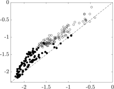
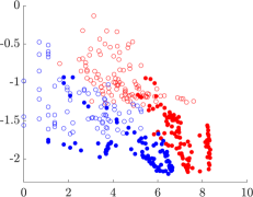
Figure 4: Variability of the expected intensity estimates $\textnormal{E}(\Lambda_{t}(A)|\mathbf{y}_{1:T})$, measured by the normalised interquantile range, $(Q_{97.5}(\Lambda_{t}(A))-Q_{2.5}(\Lambda_{t}(A)))/Q_{50}(\Lambda_{t}(A))$, for 100 different $1^{\circ}\times 1^{\circ}$ and $4^{\circ}\times 4^{\circ}$ areas $A$ ($\circ$ and $\bullet$, respectively). Left: Dry-season month against wet-season month range. Right: range against the number of fires in the same areas during dry ($\circ$, $\bullet$) and wet ($\circ$, $\bullet$) seasons.

The coefficient of variation (CV) of the intensity $\Lambda_{t}$ reported in Fig. 3 confirms the greater flexibility of the time-varying scale specifications (see also Fig. 3 and 4 in the Supplement). Since low CV values are associated with low posterior variance of $\Lambda_{t}(y)$, this measure is relevant in assessing the uncertainty, a crucial issue in spatial analysis. The CV of time-varying scale models presents higher spatial heterogeneity when compared to the constant scale models. Their CV is naturally lower (dark grey indicates values below 1) in areas with more fires, which suggests their latent random measures can better capture variability, possibly due to unobserved spatial factors.

To get further insights into the drivers of the uncertainty of $\Lambda_{t}$ across time and space, we report in Fig. 4 the normalised interquantile range defined as $(Q_{97.5}(\Lambda_{t}(A))-Q_{2.5}(\Lambda_{t}(A)))/Q_{50}(\Lambda_{t}(A))$, for several sub-regions $A\subset\mathbb{Y}$. The left plot shows that the uncertainty is larger during the dry season than during the wet season since all points lay above the $45^{\circ}$ line. Also, larger regions (dots) have lower uncertainty than smaller regions (circles) as more observations are available. This is confirmed by comparing the uncertainty and the number of observations per sub-region. The right plot shows that within each season, the uncertainty decreases when the number of observations increases. Figure 6 in the Supplement reports the results for different sizes of the sub-regions.

Figure 7 in the Supplement reports the value of the function $\mathscr{R}_{t,t+h}(x,y)$, for $t=3$ (March) and $t=11$ (November) at different locations and horizons ($h=0,1,3$). In each plot, there are areas with clustering features, that is, $\mathscr{R}_{t,t+h}(x,y)>1$, at a distance of $4^{\circ}$ from the centre $x$ (red shades), meaning that fires are likely to occur jointly at location $x$. Other areas exhibit regularity, that is, $\mathscr{R}_{t,t+h}(x,y)<1$ (white and blue shades). Overall there is evidence of spatial heterogeneity and deviation from the standard Poisson process. The local aggregation features decrease as the horizon $h$ increases and do not change across dry and wet season months (e.g. November).

A Proofs

In this Section, we provide all the proofs of the results presented in the main text.

of Proposition 1.

By eq. (2), for any $f\in\textnormal{BM}_{+}(\Theta)$ one has

$$\textnormal{E}\Big{(}e^{-\int_{\Theta}f(\theta)\>W_{t+1}(\mathrm{d}\theta)}\mid V_{t+1}\Big{)}=\exp\Big{(}-\!\!\int_{\Theta}\log(1+c_{t+1}f(\theta))\>H(\mathrm{d}\theta)-\!\!\int_{\Theta}\log(1+c_{t+1}f(\theta))\>V_{t+1}(\mathrm{d}\theta)\Big{)}.$$ (S.21)

Recall now that a Poisson random measure $V$ on $\Theta$ with intensity measure $H$ has Laplace functional

$$\mathcal{L}_{V}(f)=\textnormal{E}\Big{(}e^{-\int_{\Theta}f(\theta)V(\mathrm{d}\theta)}\Big{)}=\exp\Big{(}-\!\!\int_{\Theta}\big{(}1-e^{-f(\theta)}\big{)}\>H(\mathrm{d}\theta)\Big{)},\qquad f\in\textnormal{BM}_{+}(\Theta).$$ (S.22)

By iterated expectations and using eq. (S.21) together with eq. (S.22), we have

$$\textnormal{E}\Big{(} e^{-\int_{\Theta}f(\theta)\>W_{t+1}(\mathrm{d}\theta)}\mid W_{t}\Big{)}=\textnormal{E}\Big{(}\textnormal{E}\Big{(}\exp\Big{(}-\int_{\Theta}f(\theta)\>W_{t+1}(\mathrm{d}\theta)\Big{)}\mid V_{t+1}\Big{)}\mid W_{t}\Big{)}$$

$$=\exp\Big{(}-\!\!\int_{\Theta}\log(1+c_{t+1}f(\theta))\>H(\mathrm{d}\theta)\Big{)}\times\textnormal{E}\Big{(}\exp\Big{(}-\!\!\int_{\Theta}\log(1+c_{t+1}f(\theta))\>V_{t+1}(\mathrm{d}\theta)\Big{)}\mid W_{t}\Big{)}$$

$$=\exp\Big{(}-\!\!\int_{\Theta}\log(1+c_{t+1}f(\theta))\>H(\mathrm{d}\theta)\Big{)}\times\exp\Big{(}-\!\beta_{t+1}\!\int_{\Theta}\Big{(}1-e^{-\log(1+c_{t+1}f(\theta))}\Big{)}\>W_{t}(\mathrm{d}\theta)\Big{)}$$

$$=\exp\Big{(}-\!\!\int_{\Theta}\log(1+c_{t+1}f(\theta))\>H(\mathrm{d}\theta)-\!\!\int_{\Theta}\frac{\beta_{t+1}c_{t+1}f(\theta)}{1+c_{t+1}f(\theta)}\>W_{t}(\mathrm{d}\theta)\Big{)}.$$

By Definition 1, the thesis follows. ∎

of Proposition 2.

From eq. (S.21) one observes that the conditional law of $W_{t+1}$ given $V_{t+1}$ of the state space representation in eq. (5) is equivalent to

$$W_{t+1}\mid V_{t+1}\stackrel{{\scriptstyle\mathscr{L}}}{{=}}W_{t+1}^{(I)}+W_{t+1}^{(U)},$$

where $W_{t+1}^{(I)}$ is independent from $W_{t+1}^{(U)}$ and

$$W_{t+1}^{(I)}\mid V_{t+1}\sim\mathcal{G}a\textnormal{P}\big{(}W_{t+1}^{(I)}\mid H,c_{t+1}^{-1}\big{)}\qquad W_{t+1}^{(U)}\mid V_{t+1}\sim\mathcal{G}a\textnormal{P}\big{(}W_{t+1}^{(U)}\mid V_{t+1},c_{t+1}^{-1}\big{)}.$$

Recalling that $V_{t+1}\mid W_{t}\sim PP(V_{t+1}\mid\beta_{t+1}W_{t})$, conditionally on $W_{t}=\sum_{i\geq 1}w_{i,t}\delta_{\theta_{i,t}}$ one can write

$$V_{t+1}=\sum_{i\geq 1}v_{i,t+1}\delta_{\theta_{i,t}},\quad\quad v_{i,t+1}\sim\mathcal{P}oi(v_{i,t+1}\mid\beta_{t+1}w_{i,t})$$

and

$$W_{t+1}^{(U)}\mid V_{t+1}\stackrel{{\scriptstyle\mathscr{L}}}{{=}}\sum_{i\geq 1}w_{i,t+1}^{(U)}\delta_{\theta_{i,t}},$$

where the weights are distributed as

$$w_{i,t+1}^{(U)}\sim\begin{cases}\delta_{0}\big{(}w_{i,t+1}^{(U)}\big{)}&\text{ if }v_{i,t+1}=0\\[5.0pt] \mathcal{G}a\big{(}w_{i,t+1}^{(U)}\mid v_{i,t+1},c_{t+1}^{-1}\big{)}&\text{ if }v_{i,t+1}>0,\end{cases}$$

for $i=1,2,\ldots$, which is equivalent to the statement. ∎

of Proposition 3.

It is enough to show that $\textnormal{E}(N_{t}(B))<+\infty$ for every bounded $B$, which clearly yields that $\textnormal{pr}\{N_{t}(B)<+\infty\}=1$, that is, $N_{t}$ is a locally finite random measure. Using eq. (9) in Proposition 7 with $g_{1}(\theta)=\kappa_{t}\int_{B}K_{\phi}(y,\theta)\ell(\mathrm{d}y)$, the above expectation is finite thanks to eq. (7). ∎

of Proposition 4.

Consider the case $h=2$. By iterated use of Proposition 1 and iterated expectations one obtains

$$\textnormal{E}\Big{(} e^{-\int_{\Theta}f(\theta)\>W_{t+2}(\mathrm{d}\theta)}\mid W_{t}\Big{)}=\textnormal{E}\Big{(}\textnormal{E}\Big{(}\exp\Big{(}-\int_{\Theta}f(\theta)\>W_{t+2}(\mathrm{d}\theta)\Big{)}\mid W_{t+1}\Big{)}\mid W_{t}\Big{)}$$

$$=\exp\Big{(}-\!\!\int_{\Theta}\log\big{(}1+c_{t+2}f(\theta)\big{)}\>H(\mathrm{d}\theta)\Big{)}\times\textnormal{E}\Big{(}\exp\Big{(}-\!\int_{\Theta}\frac{\rho_{t+2}f(\theta)}{1+c_{t+2}f(\theta)}\>W_{t+1}(\mathrm{d}\theta)\Big{)}\mid W_{t}\Big{)}$$

$$=\exp\Big{(}-\!\!\int_{\Theta}\log\big{(}1+c_{t+2}f(\theta)\big{)}\>H(\mathrm{d}\theta)\Big{)}\times\exp\Big{(}-\!\int_{\Theta}\frac{\rho_{t+1}\frac{\rho_{t+2}f(\theta)}{1+c_{t+2}f(\theta)}}{1+c_{t+1}\frac{\rho_{t+2}f(\theta)}{1+c_{t+2}f(\theta)}}\>W_{t}(\mathrm{d}\theta)\Big{)}$$

$$\quad\times\exp\Big{(}-\!\!\int_{\Theta}\log\Big{(}1+c_{t+1}\frac{\rho_{t+2}f(\theta)}{1+c_{t+2}f(\theta)}\Big{)}\>H(\mathrm{d}\theta)\Big{)}$$

$$=\exp\Big{(}-\!\!\int_{\Theta}\log\big{(}1+(c_{t+2}+c_{t+1}\rho_{t+2})f(\theta)\big{)}\>H(\mathrm{d}\theta)$$

$$\qquad\quad-\!\int_{\Theta}\dfrac{\rho_{t+2}\rho_{t+1}f(\theta)}{1+(c_{t+2}+\rho_{t+2}c_{t+1})f(\theta)}\>W_{t}(\mathrm{d}\theta)\Big{)}.$$

The general case $h>2$ follows by iterating the same argument. ∎

of Corollary 1.

It can be easily proved that if $M\sim\textnormal{Nc}\mathcal{G}a\textnormal{P}(M\mid H,\beta W,c^{-1})$, then

$$\textnormal{E}(M(A))=cH(A)+c\beta W(A).$$

By Proposition 4, the thesis follows. ∎

of Proposition 5.

By assuming $c_{t}=c$, $\beta_{t}=\beta,\forall\,t$, one has $\rho_{t+h|t}=\rho^{h}$ and $c_{t+h|t}=c(1-\rho^{h})/(1-\rho)$ for any $h\geq 1$. Then, by Proposition 4 one gets

$$\lim_{h\to+\infty}\textnormal{E}\Big{(}e^{-\int_{\Theta}f(\theta)\>W_{t+h}(\mathrm{d}\theta)}\mid W_{t}\Big{)} =\lim_{h\to+\infty}\!\exp\Bigg{(}-\!\!\int_{\Theta}\log\Big{(}1+\frac{c(1-\rho^{h})}{1-\rho}f(\theta)\Big{)}\>H(\mathrm{d}\theta)$$

$$\qquad\qquad-\!\!\int_{\Theta}\dfrac{\rho^{h}f(\theta)}{1+\frac{c(1-\rho^{h})}{1-\rho}f(\theta)}\>W_{t}(\mathrm{d}\theta)\Bigg{)}.$$

Under the assumption $\rho<1$, the exponent of the second term converges to $0$ by the dominated convergence theorem. In fact, for any $f\in\textnormal{BM}_{+}(\Theta)$ and any $h\geq 1$,

$$f_{h}(\theta)\coloneqq\rho^{h}f(\theta)\Bigg{(}1+\frac{c(1-\rho^{h})}{1-\rho}f(\theta)\Bigg{)}^{-1}\leq\rho^{h}f(\theta)\leq f(\theta),\quad\forall\,\theta\in\Theta,\>\forall\,h\geq 1$$

and clearly $\lim_{h\to+\infty}f_{h}(\theta)=0$ for any $\theta$. Analogously, we can establish a bound for the argument of the logarithm in the first exponent as $1+(c(1-\rho^{h}))(1-\rho)^{-1}f(\theta)\leq 1+c(1-\rho)^{-1}f(\theta)$ and clearly $\lim_{h\to+\infty}1+(c(1-\rho^{h}))(1-\rho)^{-1}f(\theta)=1+c(1-\rho)^{-1}f(\theta)$. Therefore

$$\lim_{h\to+\infty}\textnormal{E}\Big{(}\exp\Big{(}-\int_{\Theta}f(\theta)\>W_{t+h}(\mathrm{d}\theta)\Big{)}\mid W_{t}\Big{)}=\exp\Big{(}-\!\!\int_{\Theta}\log\Big{(}1+\frac{c}{1-\rho}f(\theta)\Big{)}\>H(\mathrm{d}\theta)\Big{)}.$$

Finally, when $W_{t}\sim\mathcal{G}a\textnormal{P}(W_{t}\mid H,(1-\rho)/c)$, we can prove that the random measure $W_{t+1}$ follows the same law as $W_{t}$ by using Proposition 1, as follows:

$$\textnormal{E}\Big{(}\textnormal{E}\Big{(} e^{-\int_{\Theta}f(\theta)\>W_{t+1}(\mathrm{d}\theta)}\mid W_{t}\Big{)}\Big{)}=\exp\Big{(}-\!\!\int_{\Theta}\log\big{(}1+cf(\theta)\big{)}\>H(\mathrm{d}\theta)\Big{)}$$

$$\times\textnormal{E}\Big{(}\exp\Big{(}-\int_{\Theta}\frac{\rho f(\theta)}{1+cf(\theta)}\>W_{t}(\mathrm{d}\theta)\Big{)}\Big{)}$$

$$=\exp\Big{(}-\!\!\int_{\Theta}\log\big{(}1+cf(\theta)\big{)}\>H(\mathrm{d}\theta)-\!\!\int_{\Theta}\log\Big{(}1+\frac{c}{1-\rho}\frac{\rho f(\theta)}{1+cf(\theta)}\Big{)}\>H(\mathrm{d}\theta)\Big{)}$$

$$=\exp\Big{(}-\!\!\int_{\Theta}\log\Big{(}1+\frac{c}{1-\rho}f(\theta)\Big{)}\>H(\mathrm{d}\theta)\Big{)}.$$

∎

of Proposition 6.

Since $\Lambda_{t}(\mathrm{d}y)=\int_{\Theta}K_{\phi}(y,\theta)\>W_{t}(\mathrm{d}\theta)\ell(\mathrm{d}y)$, one has:

$$\begin{split}\mathcal{L}_{N_{t}}(f)&=\textnormal{E}\Big{(}\exp\Big{(}-\!\int_{\mathbb{Y}}\Big{(}1-e^{-f(y)}\Big{)}\>\int_{\Theta}K_{\phi}(y,\theta)\>W_{t}(\mathrm{d}\theta)\ell(\mathrm{d}y)\Big{)}\Big{)}\\ &=\textnormal{E}\Big{(}\exp\Big{(}-\!\int_{\Theta}g(\theta)\>W_{t}(\mathrm{d}\theta)\Big{)}\Big{)}=\mathcal{L}_{W_{t}}(g),\end{split}$$

where

$$g(\theta)\coloneqq\int_{B_{f}}\Big{(}1-e^{-f(y)}\Big{)}K_{\phi}(y,\theta)\>\ell(\mathrm{d}y),$$

and $B_{f}\subset\mathbb{Y}$ is the support of $f$ which is bounded by assumption. Since $f$ is also bounded $\int_{\Theta}g(\theta)H(\mathrm{d}\theta)\leq\int_{\Theta}\int_{B_{f}}K_{\phi}(y,\theta)\>\ell(\mathrm{d}y)H(\mathrm{d}\theta)<+\infty$ by eq. (7). This also yields

$$\mathcal{I}(g)\coloneqq\int_{\Theta}\log\Big{(}1+\dfrac{c}{1-\rho}g(\theta)\Big{)}\>H(\mathrm{d}\theta)<+\infty.$$

Hence $\mathcal{L}_{N_{\infty}}(f)$ is well-defined and $\exp(-\mathcal{I}(g))=\mathcal{L}_{N_{\infty}}(f)=\mathcal{L}_{W_{\infty}}(g)$ when $W_{\infty}\sim\mathcal{G}a\textnormal{P}(W_{\infty}\mid H,(1-\rho)/c)$. At this stage, one gets that if $W_{t}$ is stationary, then process $N_{t}$ is stationary in the sense that $N_{t}\stackrel{{\scriptstyle\mathscr{L}}}{{=}}N_{\infty}$. To prove the first part of the statement, choose $A_{\epsilon}\subset\Theta$ bounded such that $\mathcal{I}(g\mathds{1}\{A_{\epsilon}^{c}\})\leq\epsilon$, which is possible for every $\epsilon$ given $f$ since $\mathcal{I}(g)<+\infty$. Using eq. (9) and again eq. (7), one can also choose $A_{\epsilon}$ in such a way $\textnormal{E}(\int_{A_{\epsilon}^{c}}W_{t}(\mathrm{d}\theta))\leq\epsilon$ for every $t$. Now define $g^{\epsilon}(\theta)=g(\theta)\mathds{1}\{\theta\in A_{\epsilon}\}$ and write

$$|\mathcal{L}_{N_{t}}(f)-\mathcal{L}_{N_{\infty}}(f)|\leq|\mathcal{L}_{W_{t}}(g)-\mathcal{L}_{W_{t}}(g^{\epsilon})|+|\mathcal{L}_{W_{t}}(g^{\epsilon})-\mathcal{L}_{W_{\infty}}(g^{\epsilon})|+|\mathcal{L}_{W_{\infty}}(g^{\epsilon})-\mathcal{L}_{W_{\infty}}(g)|.$$

When $t\rightarrow+\infty$ one has that $|\mathcal{L}_{W_{t}}(g^{\epsilon})-\mathcal{L}_{W_{\infty}}(g^{\epsilon})|$ goes to zero by Proposition 5, and using the conditions $\textnormal{E}(\int_{A_{\epsilon}^{c}}W_{t}(\mathrm{d}\theta))\leq\epsilon$ and $\mathcal{I}(g\mathds{1}\{A_{\epsilon}^{c}\})\leq\epsilon$ one gets $|\mathcal{L}_{W_{t}}(g)-\mathcal{L}_{W_{t}}(g^{\epsilon})|+|\mathcal{L}_{W_{\infty}}(g^{\epsilon})-\mathcal{L}_{W_{\infty}}(g)|\leq\epsilon$. ∎

of Proposition 7.

By Proposition 3 one has that $W_{t}$ given $W_{1}$ has distribution $\textnormal{Nc}\mathcal{G}a\textnormal{P}(H,\beta_{t|1}W_{1},c_{t|1}^{-1})$, which is a CRM with Lévy measure $\mu(\mathrm{d}w,\mathrm{d}\theta)=w^{-1}e^{-w/c_{t|1}}\>\mathrm{d}wH(\mathrm{d}\theta)+\beta_{t|1}/c_{t|1}e^{-w/c_{t|1}}\mathrm{d}wW_{1}(\mathrm{d}\theta)$, see eq. (3). By eq. (4), one has the representation $W_{t}(g_{i})=\int_{\mathds{R}_{+}\times\Theta}g_{i}(\theta)w\>M(\mathrm{d}w\mathrm{d}\theta)$ ($i=1,2$), with $M\sim\textnormal{PP}(M\mid\mu)$. Now recall that, if $f_{1}$ and $f_{2}$ are measurable functions, then

$$\textnormal{E}\Big{(}\int_{\mathds{R}_{+}\times\Theta}f_{1}(w,\theta)\>M(\mathrm{d}w\mathrm{d}\theta)\Big{)}=\int_{\Re_{+}\times\Theta}f(w,\theta)\>\mu(\mathrm{d}w\mathrm{d}\theta),$$ (S.23)

$$\textnormal{cov}\Big{(}\int_{\Re_{+}\times\Theta}\!f_{1}(w,\theta)\>M(\mathrm{d}w\mathrm{d}\theta),\int_{\mathds{R}_{+}\times\Theta}\!f_{2}(w^{\prime},\theta^{\prime})\>M(\mathrm{d}w^{\prime}\mathrm{d}\theta^{\prime})\Big{)}=$$

$$\hskip 150.69397pt=\!\int_{\mathds{R}_{+}\times\Theta}\!f_{1}(w,\theta)f_{2}(w,\theta)\>\mu(\mathrm{d}w\mathrm{d}\theta),$$ (S.24)

provided the integrals on the right-hand side are well-defined (see, e.g. Last and Penrose,, 2018, Campbell’s formula in Proposition 2.7 and eq. 4.26). The expression (9) follows from eq. (S.23). As for eq. (10), we start with the elementary identity:

$$\textnormal{cov}(W_{t}(g_{1}),W_{t}(g_{2}))=\textnormal{E}(\textnormal{cov}(W_{t}(g_{1}),W_{t}(g_{2})\mid W_{1}))+\textnormal{cov}(\textnormal{E}(W_{t}(g_{1})\mid W_{1}),\textnormal{E}(W_{t}(g_{2})\mid W_{1})).$$

Using Proposition 1 with $t=1$ and $h=t-1$ one gets $\textnormal{E}(W_{t}(g_{i})\mid W_{1})=c_{t|1}H(g_{i})+\rho_{t|1}W_{1}(g_{i})$ and hence

$$\textnormal{cov}(\textnormal{E}(W_{t}(g_{1})\mid W_{1}),\textnormal{E}(W_{t}(g_{2})|W_{1}))=\rho_{t|1}^{2}\textnormal{cov}(W_{1}(g_{1}),W_{1}(g_{2})).$$

It remains to compute $\textnormal{cov}(W_{t}(g_{1}),W_{t}(g_{2})|W_{1})$. Using eq. (S.24) with $f_{i}(w,\theta)=wg_{i}(\theta)$ one obtains

$$\begin{split}\textnormal{cov}(W_{t}(g_{1}),W_{t}(g_{2})\mid W_{1})&=\int_{\mathds{R}_{+}\times\Theta}g_{1}(\theta)g_{2}(\theta)w^{2}\>\mu(\mathrm{d}w\mathrm{d}\theta)\\ &=c_{t|1}^{2}\int_{\Theta}g_{1}(\theta)g_{1}(\theta)\big{(}H(\mathrm{d}\theta)+2\beta_{t|1}W_{1}(\mathrm{d}\theta)\big{)}.\end{split}$$

Equation (10) follows. Using Proposition 1 one gets

$$\begin{split}\textnormal{E}(W_{t}(g_{1})W_{t+h}(g_{2}))&=\textnormal{E}(W_{t}(g_{1})\textnormal{E}(W_{t+h}(g_{2})\mid W_{t}))\\ &=c_{t+h|t}\textnormal{E}(W_{t}(g_{1}))\int_{\Theta}g_{2}(\theta)H(\mathrm{d}\theta)+\rho_{t+h|t}\textnormal{E}(W_{t}(g_{1})W_{t}(g_{2}))\end{split}$$ (S.25)

and

$$\textnormal{E}(W_{t}(g_{1}))\,\textnormal{E}(W_{t+h}(g_{2}))=c_{t+h|t}\textnormal{E}(W_{t}(g_{1}))\,\int_{\Theta}g_{2}(\theta)H(\mathrm{d}\theta)+\rho_{t+h|t}\textnormal{E}(W_{t}(g_{2}))\textnormal{E}(W_{t}(g_{1})).$$

Combining these two identities, eq. (11) follows. ∎

of Proposition 8.

Note that the expressions for $\mathfrak{D}^{(1)}_{t}(y)$, $\mathfrak{D}^{(2)}_{t}(y_{1},y_{2})$ and $\mathfrak{D}^{(2)}_{t,t+h}(y_{1},y_{2})$ are well defined $\ell$-almost everywhere by $(H_{1})$-$(H_{3})$. In addition, integrals in eq. (12) for these functions are also well-defined for bounded sets. Starting from eq. (13), eq. (8) follows by (9) with $g(\theta)=\kappa_{t}K_{\phi}(y,\theta)$ and (8) follows by (S.25) with $g_{1}(\theta)=\kappa_{t}K_{\phi}(y_{1},\theta)$ and $g_{2}(\theta)=\kappa_{t+h}K_{\phi}(y_{2},\theta)$. Similarly eq. (14) follows by eq. (9)-(10) using the elementary identity $\textnormal{E}(\lambda_{t}(y_{1})\lambda_{t}(y_{2}))=\textnormal{cov}(\lambda_{t}(y_{1}),\lambda_{t}(y_{2}))+\textnormal{E}(\lambda_{t}(y_{1}))\textnormal{E}(\lambda_{t}(y_{2}))$. Note that eq. (14) can also be deduced using Proposition 5.1 in Møller and Waagepetersen, (2003), which states that in a Cox process directed by a Poisson process with intensity measure $\mu$ and kernel $k$, the second-order product density $\mathfrak{D}^{(2)}(y_{1},y_{2})$ satisfies

$$\begin{split}\mathfrak{D}^{(2)}(y_{1},y_{2})&=\int_{\Re_{+}\times\Theta}wk(\theta,y_{1})\mu(\mathrm{d}w\mathrm{d}\theta)\int_{\Re_{+}\times\Theta}wk(\theta,y_{2})\mu(\mathrm{d}w\mathrm{d}\theta)\\ &+\int_{\Re_{+}\times\Theta}w^{2}k(\theta,y_{1})k(\theta,y_{2})\mu(\mathrm{d}w\mathrm{d}\theta).\end{split}$$ (S.26)

Since conditionally on $W_{1}$, $N_{t}$ is a Cox process directed by a Poisson process with intensity $\mu(\mathrm{d}w,\mathrm{d}\theta)=\kappa_{t}w^{-1}e^{-w/c_{t|1}}\>\mathrm{d}wH(\mathrm{d}\theta)+\kappa_{t}\beta_{t|1}/c_{t|1}e^{-w/c_{t|1}}\mathrm{d}wW_{1}(\mathrm{d}\theta)$, eq. (14) follows by conditioning and elementary computations starting from eq. (S.26). ∎

of Proposition 9.

By Proposition 5, $W_{t}\sim\mathcal{G}a\textnormal{P}(W_{t}\mid H,(1-\rho)/c)$. Equation (15) follows immediately from Proposition 8. As for the second-order product density, one can use the expression recalled in eq. (8) where now the Lévy measure of $W_{t}$ is $\mu(\mathrm{d}w\mathrm{d}\theta)=w^{-1}e^{-c^{*}w}\mathrm{d}wH(\mathrm{d}\theta)$, with $c^{*}=(1-\rho)/c$. ∎

of Corollary 2.

The proof follows by combining eq. (12) with Proposition 8. As an alternative proof, recall that if $M\sim PP(M\mid\mu)$ then $E(M(B_{1}))=\mu(B_{1})$ and $\textnormal{E}(M(B_{1})M(B_{2}))=\mu(B_{1})\mu(B_{2})+\mu(B_{1}\cap B_{1})$ (see, e.g. Last and Penrose,, 2018, Campbell’s formula in Proposition 2.7 and eq. 4.26). Hence, since $N_{t}\mid W_{t}\sim PP(N_{t}\mid\Lambda_{t})$ one gets

$$\textnormal{cov}(N_{t}(B_{1}),N_{t}(B_{2}))=\textnormal{cov}(\Lambda_{t}(B_{1}),\Lambda_{t}(B_{2}))+\textnormal{E}\big{(}\Lambda_{t}(B_{1}\cap B_{2})\big{)}.$$ (S.27)

Since for any set $B\subset\mathbb{Y}$, one has $\Lambda_{t}(B)=\kappa_{t}\int_{\Theta}K_{\phi}(B,\theta)W_{t}(\mathrm{d}\theta)$, by (9) with $g(\theta)=\kappa_{t}K_{\phi}(B_{1}\cap B_{2},\theta)$ it follows

$$\textnormal{E}(\Lambda_{t}(B_{1}\cap B_{2}))=\kappa_{t}c_{t|1}\int_{\Theta}K_{\phi}(B_{1}\cap B_{2},\theta)(H(\mathrm{d}\theta)+\beta_{t|1}\bar{W}_{1}(\mathrm{d}\theta)).$$

Moreover, by Proposition 7 with $g_{1}(\theta)=\kappa_{t}K_{\phi}(B_{1},\theta)$ and $g_{2}(\theta)=\kappa_{t}K_{\phi}(B_{2},\theta)$ one obtains

$$\begin{split}\textnormal{cov}(\Lambda_{t}(B_{1}),\Lambda_{t}(B_{2}))&=\kappa_{t}^{2}c_{t|1}^{2}\int_{\Theta}K_{\phi}(B_{1},\theta)K_{\phi}(B_{2},\theta)(H(\mathrm{d}\theta)+2\beta_{t|1}\bar{W}_{1}(\mathrm{d}\theta))\\ &+\kappa_{t}^{2}\rho_{t|1}^{2}\textnormal{cov}\Big{(}\int_{\Theta}K_{\phi}(B_{1},\theta)W_{1}(\mathrm{d}\theta),\int_{\Theta}K_{\phi}(B_{2},\theta)W_{1}(\mathrm{d}\theta)\Big{)}.\end{split}$$

Collecting all the terms, the statement for $h=0$ follows. As for $h\geq 1$

$$\begin{split}\textnormal{E}(N_{t}(B_{1})N_{t+h}(B_{2}))&=\textnormal{E}\big{(}\textnormal{E}(N_{t}(B_{1})N_{t+h}(B_{2})\mid W_{t},W_{t+h})\big{)}\\ &=\textnormal{E}(\Lambda_{t}(B_{1})\Lambda_{t+h}(B_{2})).\end{split}$$

Since $\textnormal{E}(N_{t}(B_{1}))=\textnormal{E}(\Lambda_{t}(B_{1}))$ and $\textnormal{E}(N_{t+h}(B_{2}))=\textnormal{E}(\Lambda_{t+h}(B_{2}))$, one gets

$$\textnormal{cov}(N_{t}(B_{1}),N_{t+h}(B_{2}))=\textnormal{cov}(\Lambda_{t}(B_{1}),\Lambda_{t+h}(B_{2}))=\textnormal{cov}(W_{t}(g_{1}),W_{t+h}(g_{2})),$$ (S.28)

for $g_{1}(\theta)=\kappa_{t}K_{\phi}(B_{1},\theta)$ and $g_{2}(\theta)=\kappa_{t+h}K_{\phi}(B_{2},\theta)$. By Proposition (9), $\textnormal{cov}(W_{t}(g_{1}),W_{t+h}(g_{2}))=\rho_{t+h|t}\textnormal{cov}(W_{t}(g_{1}),W_{t}(g_{2}))$ and the thesis follows also for $h\geq 1$. ∎

of Corollary 3.

Start by recalling the relationship $\textnormal{E}(N_{t}(B_{1}))=\textnormal{E}(\Lambda_{t}(B_{1}))=\kappa_{t}\textnormal{E}\big{(}\int_{\Theta}K_{\phi}(B_{1},\theta)W_{t}(\mathrm{d}\theta)\big{)}$. Under the stated assumptions, it follows that $W_{t}\sim\mathcal{G}a\textnormal{P}(W_{t}\mid H,(1-\rho)/c)$ and $W_{t}\sim\mathcal{G}a\textnormal{P}(W_{t}\mid H,(1-\rho)/c)$, cf. Proposition 5, thus proving the first statement. If $h=0$, by eq. (S.27) one has $\textnormal{cov}(N_{t}(B_{1}),N_{t+h}(B_{2}))=\textnormal{cov}(W_{t}(g_{1}),W_{t}(g_{2}))+\textnormal{E}\big{(}W_{t}(g_{1,2})\big{)}$, where $g_{1}(\theta)=\kappa_{t}K_{\phi}(B_{1},\theta)$, $g_{2}(\theta)=\kappa_{t}K_{\phi}(B_{2},\theta)$, and $g_{1,2}(\theta)=\kappa_{t}K_{\phi}(B_{1}\cap B_{2},\theta)$. Since $W_{t}\sim\mathcal{G}a\textnormal{P}(W_{t}\mid H,(1-\rho)/c)$, the second part of the statement for $h=0$ follows using eq. (S.24). To conclude, assume $h\geq 1$ and use eq. (S.28) to write $\textnormal{cov}(N_{t}(B_{1}),N_{t+h}(B_{2}))=\textnormal{cov}(W_{t}(g_{1}),W_{t+h}(g_{2}))$, with $g_{1}(\theta)=\kappa_{t}K_{\phi}(B_{1},\theta)$ and $g_{2}(\theta)=\kappa_{t+h}K_{\phi}(B_{2},\theta)$. By Proposition (9), $\textnormal{cov}(W_{t}(g_{1}),W_{t+h}(g_{2}))=\rho_{t+h|t}\textnormal{cov}(W_{t}(g_{1}),W_{t}(g_{2}))$ and the claim follows using $W_{t}\sim\mathcal{G}a\textnormal{P}(W_{t}\mid H,(1-\rho)/c)$ and eq. (S.24). ∎

of Proposition 10.

The unconditional moments of $N_{t}(B)$ follow from the moments of $\Lambda_{t}$. Since $N_{t}(B)\mid\Lambda_{t}\sim\mathcal{P}oi(N_{t}(B)\mid\Lambda_{t}(B))$ and the $m$th moment of a Poisson random variable of parameter $\lambda$ is $\sum_{j=1}^{m}S_{m,j}\lambda^{j}$, then

$$\textnormal{E}\big{(}N_{t}(B)^{m}\big{)}=E\Big{(}\textnormal{E}\big{(}N_{t}(B)^{m}\mid\Lambda_{t}\big{)}\Big{)}=\textnormal{E}\Big{(}\sum_{j=1}^{m}S_{m,j}\Lambda_{t}(B)^{j}\Big{)}.$$ (S.29)

To prove eq. (17), starting from eq. (S.29), one needs to compute $\textnormal{E}\big{(}\Lambda_{t}(B)^{j}\big{)}$. Since we are assuming that $W_{t}\sim\mathcal{G}a\textnormal{P}(W_{t}\mid H,(1-\rho)/c)$, $W_{t}$ is a CRM with Lévy measure $\mu(\mathrm{d}w\mathrm{d}\theta)=w^{-1}e^{-c^{*}w}\mathrm{d}wH(\mathrm{d}\theta)$, where $c^{*}=(1-\rho)/c$. By eq. (4)

$$\Lambda_{t}(B)=\kappa_{t}\int_{\Theta}K_{\phi}(B,\theta)\>W_{t}(\mathrm{d}\theta)=\kappa_{t}\int_{\mathds{R}_{+}\times\Theta}K_{\phi}(B,\theta)w\>M(\mathrm{d}w\mathrm{d}\theta),$$

where $M\sim\textnormal{PP}(M\mid\mu)$. For $M\sim\textnormal{PP}(M\mid\mu)$, following Bassan and Bona, (1990), one has

$$\textnormal{E}\Big{(}\Big{(}\int_{\mathds{R}_{+}\times\Theta}K_{\phi}(B,\theta)w\>M(\mathrm{d}w\mathrm{d}\theta)\Big{)}^{j}\Big{)}=\sum_{\begin{subarray}{c}\ell_{1},\dots,\ell_{j}\geq 0\\ \sum_{r=1}^{j}r\ell_{r}=j\end{subarray}}c(\ell_{1},\dots,\ell_{j})\prod_{r=1}^{j}J_{r}(B)^{\ell_{r}},$$

which concludes the proof. ∎

B Posterior full conditional distributions

In this section, we provide a description of the posterior full conditional distributions of the parameters and the algorithms used to draw samples from them. Let us first define the collection of measures $\mathbf{W}=\{W_{1},\ldots,W_{T}\}$, $\mathbf{Z}=\{Z_{1},\ldots,Z_{T}\}$, $\mathbf{Y}=\{y_{1},\ldots,y_{T}\}$, and $\mathbf{N}^{y}=\{N_{1}^{y},\ldots,N_{T}^{y}\}$. Finally, let us recall that $\bm{\alpha}=\{\alpha_{1},\ldots,\alpha_{N^{g}}\}$, $\mathbf{c}=\{c_{1},\ldots,c_{T}\}$, $\mathbf{y}_{1:T}=\{y_{1},\ldots,y_{T}\}$, $\mathbf{w}_{1:T}=\{w_{1},\ldots,w_{T}\}$ and $\mathbf{z}_{1:T}=\{z_{1},\ldots,z_{T}\}$.

B.1 Sampling the parameters $\psi$

The parameters $\bm{\psi}$ given $\mathbf{y}_{1:T},\mathbf{z}_{1:T}$, and $\mathbf{w}_{1:T}$ are drawn from their full conditional distributions by adaptive Metropolis-Hastings. Details are given below.

The full conditional posterior of the spatial shape parameters $\alpha_{j}$, $j=1,\ldots,N^{g}$ is

$$\alpha_{j}\mid\mathbf{W},\beta,\mathbf{c},\gamma\propto\mathcal{G}a(\alpha_{j}\mid\underline{a}_{\alpha},\gamma\underline{b}_{\alpha})\prod_{t=1}^{T}\textnormal{Nc}\mathcal{G}a(w_{j,t}\mid\alpha_{j},\beta w_{j,t-1},c_{t}^{-1}),$$

which can be sampled by using an adaptive random walk Metropolis-Hastings (RWMH) step with a Lognormal proposal (e.g., see Andrieu and Thoms,, 2008; Atchadé and Rosenthal,, 2005).

The full conditional posterior of the shape parameter $\beta$ is

$$\beta\mid\mathbf{W},\bm{\alpha},\mathbf{c},\gamma\propto\mathcal{G}a(\beta\mid\underline{a}_{\beta},\gamma\underline{b}_{\beta})\prod_{t=1}^{T}\prod_{j=1}^{N^{g}}\textnormal{Nc}\mathcal{G}a(w_{j,t}\mid\alpha_{j},\beta w_{j,t-1},c_{t}^{-1}),$$

which can be sampled by using an adaptive RWMH step with a Lognormal proposal.

The full conditional posterior of the constant scale parameter $c$ is

$$c\mid\mathbf{W},\bm{\alpha},\beta\propto\mathcal{G}a(c\mid\underline{a}_{c},\underline{b}_{c})\prod_{t=1}^{T}\prod_{j=1}^{N^{g}}\textnormal{Nc}\mathcal{G}a(w_{j,t}\mid\alpha_{j},\beta w_{j,t-1},c^{-1}),$$

which can be sampled by using an adaptive RWMH step with a Lognormal proposal.

The full conditional posterior of the scale parameters $c_{t}$, $t=1,\ldots,T$ is

$$c_{t}\mid\mathbf{W},\bm{\alpha},\beta,r\propto\mathcal{G}a(c_{t}\mid r^{2}/\underline{\sigma}^{2}_{c},r/\underline{\sigma}^{2}_{c})\prod_{j=1}^{N^{g}}\textnormal{Nc}\mathcal{G}a(w_{j,t}\mid\alpha_{j},\beta w_{j,t-1},c_{t}^{-1}),$$

which can be sampled by using an adaptive RWMH step with a Lognormal proposal.

The full conditional posterior of the hierarchical scale parameter $r$ is

$$r\mid\mathbf{c} \propto\mathcal{G}a(r\mid\underline{a}_{r},\underline{b}_{r})\prod_{t=1}^{T}\mathcal{G}a\Big{(}c_{t}\mid\frac{r^{2}}{\underline{\sigma}^{2}_{c}},\frac{r}{\underline{\sigma}^{2}_{c}}\Big{)}$$

$$\propto r^{\underline{a}_{r}-1}e^{-r\underline{b}_{r}}\prod_{t=1}^{T}\frac{1}{\Gamma\Big{(}\frac{r^{2}}{\underline{\sigma}^{2}_{c}}\Big{)}}\Big{(}\frac{r}{\underline{\sigma}^{2}_{c}}\Big{)}^{\frac{r^{2}}{\underline{\sigma}^{2}_{c}}}\>c_{t}^{\frac{r^{2}}{\underline{\sigma}^{2}_{c}}-1}\>\exp\Big{(}-\frac{r}{\underline{\sigma}^{2}_{c}}c_{t}\Big{)}$$

$$\propto r^{\underline{a}_{r}-1}\exp\Bigg{\{}-r\Big{(}\underline{b}_{r}+\sum_{t=1}^{T}\frac{c_{t}}{\underline{\sigma}^{2}_{c}}\Big{)}\Bigg{\}}\Big{(}\prod_{t=1}^{T}c_{t}\Big{)}^{\frac{r^{2}}{\underline{\sigma}^{2}_{c}}}\Bigg{\{}\frac{1}{\Gamma\Big{(}\frac{r^{2}}{\underline{\sigma}^{2}_{c}}\Big{)}}\Big{(}\frac{r}{\underline{\sigma}^{2}_{c}}\Big{)}^{\frac{r^{2}}{\underline{\sigma}^{2}_{c}}}\Bigg{\}}^{T},$$

which can be sampled by using an adaptive RWMH step with a Lognormal proposal.

Assuming monthly-specific scales $c_{t}$, that is

$$c_{t}=\begin{cases}\xi_{k},&t\bmod 12=k\wedge k\in\{1,\ldots,11\}\\ \xi_{12},&t\bmod 12=0.\end{cases}$$

We choose the hierarchical prior:

$$\xi_{k}\mid r \mathbin{\overset{iid}{\kern 0.0pt\sim}}\mathcal{G}a(\xi_{k}\mid r^{2}/\underline{\sigma}_{c}^{2},r/\underline{\sigma}_{c}^{2}),\quad k=1,\ldots,12,$$

$$r \sim\mathcal{G}a(r\mid\underline{a}_{r},\underline{b}_{r}).$$

Hence, the full conditional posterior of the monthly scale parameters $\xi_{k}$, $k=1,\ldots,12$ is

$$\xi_{k}\mid r,\bm{\alpha},\beta,\mathbf{W}\propto\mathcal{G}a(\xi_{k}\mid r^{2}/\underline{\sigma}^{2}_{c},r/\underline{\sigma}^{2}_{c})\prod_{t\in\mathcal{T}_{k}}\prod_{j=1}^{N^{g}}\textnormal{Nc}\mathcal{G}a(w_{j,t}\mid\alpha_{j},\beta w_{j,t-1},c_{t}^{-1}),$$

where $\mathcal{T}_{k}=\{t\in\{1,\ldots,T\}:t\bmod 12=k\}$, for $k=1,\ldots,11$, and $\mathcal{T}_{12}=\{t\in\{1,\ldots,T\}:t\bmod 12=0\}$ if $k=12$. We use an adaptive RWMH step to sample from this distribution.

Let $\bm{\xi}=\{\xi_{1},\ldots,\xi_{12}\}$, then the full conditional posterior of the hierarchical scale parameter $r$ is

$$r\mid\bm{\xi} \propto\mathcal{G}a(r\mid\underline{a}_{r},\underline{b}_{r})\prod_{k=1}^{12}\mathcal{G}a(\xi_{k}\mid r^{2}/\underline{\sigma}^{2}_{c},r/\underline{\sigma}^{2}_{c})$$

$$\propto r^{\underline{a}_{r}-1}e^{-r\underline{b}_{r}}\prod_{k=1}^{12}\frac{1}{\Gamma\Big{(}\frac{r^{2}}{\underline{\sigma}^{2}_{c}}\Big{)}}\Big{(}\frac{r}{\underline{\sigma}^{2}_{c}}\Big{)}^{\frac{r^{2}}{\underline{\sigma}^{2}_{c}}}\>\xi_{k}^{\frac{r^{2}}{\underline{\sigma}^{2}_{c}}-1}\>\exp\Big{(}-\frac{r}{\underline{\sigma}^{2}_{c}}\xi_{k}\Big{)}$$

$$\propto r^{\underline{a}_{r}-1}\exp\Bigg{\{}-r\Big{(}\underline{b}_{r}+\sum_{k=1}^{12}\frac{\xi_{k}}{\underline{\sigma}^{2}_{c}}\Big{)}\Bigg{\}}\Big{(}\prod_{k=1}^{12}\xi_{k}\Big{)}^{\frac{r^{2}}{\underline{\sigma}^{2}_{c}}}\Bigg{\{}\frac{1}{\Gamma\Big{(}\frac{r^{2}}{\underline{\sigma}^{2}_{c}}\Big{)}}\Big{(}\frac{r}{\underline{\sigma}^{2}_{c}}\Big{)}^{\frac{r^{2}}{\underline{\sigma}^{2}_{c}}}\Bigg{\}}^{12},$$

which can be sampled by using an adaptive RWMH step with a Lognormal proposal.

The full conditional posterior of the hierarchical scale parameter $\gamma$ is

$$\gamma\mid\bm{\alpha},\beta \propto\gamma^{\underline{a}_{\gamma}-1}\exp\big{(}-\gamma\underline{b}_{\gamma}\big{)}\gamma^{\underline{a}_{\beta}}\exp\big{(}-\beta\gamma\underline{b}_{\beta}\big{)}\prod_{j=1}^{N^{g}}\gamma^{\underline{a}_{\alpha}}\exp\big{(}-\alpha_{j}\gamma\underline{b}_{\alpha}\big{)}\propto\mathcal{G}a(\gamma\mid\overline{a}_{\gamma},\overline{b}_{\gamma}),$$

where $\overline{a}_{\gamma}=\underline{a}_{\gamma}+\underline{a}_{\beta}+N^{g}\underline{a}_{\alpha}$ and $\overline{b}_{\gamma}=\underline{b}_{\gamma}+\beta\underline{b}_{\beta}+\underline{b}_{\alpha}\sum_{j=1}^{N^{g}}\alpha_{j}$.

The full conditional posterior of the kernel bandwidth parameter $\phi$ is

$$\phi\mid\mathbf{Y},\mathbf{W},\mathbf{Z}\propto\mathcal{G}a(\phi\mid\underline{a}_{\phi},\underline{b}_{\phi})\prod_{j=1}^{N^{g}}\prod_{(i,t):z_{i,t}=j}\!\!\frac{\mathcal{N}_{2}(y_{i,t}\mid\theta_{j},\textnormal{I}_{2}\phi^{2})}{\mathcal{N}_{2}(\mathbb{Y}\mid\theta_{j},\textnormal{I}_{2}\phi^{2})},$$

which can be sampled by using an adaptive RWMH step with a Lognormal proposal.

The full conditional posterior of the temporal covariates’ coefficients $\eta$ is

$$\eta\mid\mathbf{W},\mathbf{N}^{y}\propto\mathcal{N}_{m}(\eta\mid\underline{\mu}_{\eta},\underline{\Sigma}_{\eta})\prod_{t=1}^{T}\mathcal{P}oi(N_{t}^{y}\mid\Lambda_{t}(\mathbb{Y})),$$

which can be sampled by using an adaptive RWMH step with a multivariate Lognormal proposal.

B.2 Sampling the allocation variables $\mathbf{z}_{1:T}$

The posterior distribution of the allocation variables $\mathbf{z}_{1:T}$ is easily described. For $i=1,\ldots,N_{t}^{y}$, $t=1,\ldots,T$, one has

$$\textnormal{pr}(z_{i,t}=m\mid\mathbf{y}_{1:T},\mathbf{w}_{1:T},\bm{\psi})=\frac{w_{m,t}k_{\phi}(y_{i,t},\theta_{m})}{{\Lambda}(y_{i,t})},\qquad m=1,\dots,N^{g},$$

where ${\Lambda}(y_{i,t})=\sum_{m=1}^{N^{g}}w_{m,t}k_{\phi}(y_{i,t},\theta_{m})$.

B.3 Sampling the latent states $\mathbf{w}_{1:T}$

Let $q(\cdot\mid\cdot)$ be an importance density from which the particles are generated (at $t=1$) or extended forward in time (for $t=2,\ldots,T$). Set $A_{\ell,t-1}^{k}$ to be the index of the ‘parent’ at time $t-1$ of the particle $\mathbf{w}_{\ell,1:t}^{k}$, and let $\mathcal{F}(\cdot)$ be a discrete distribution governing the resampling procedure. For $\mathcal{F}$ equal to the multinomial distribution, one obtains the standard multinomial resampling. Finally, $B_{\ell,1:T}^{k}=(B_{\ell,1}^{k},\ldots,B_{\ell,T}^{k})$ is the ancestor lineage of the $k$th particle, where $B_{\ell,T}^{k}\coloneqq k$ and $B_{\ell,t}^{k}\coloneqq A_{\ell,t}^{B_{\ell,t+1}^{k}}$ for $t=T-1,\ldots,1$. Note that $\mathbf{w}_{\ell,1:T}^{k}=(\mathbf{w}_{\ell,1}^{B_{\ell,1}^{k}},\ldots,\mathbf{w}_{\ell,T}^{B_{\ell,T}^{k}})$ for all $k$. The Sequential Monte Carlo algorithm is:

1. Let $\mathbf{w}_{\ell,1:T}=(\mathbf{w}_{\ell,1}^{B_{\ell,1}},\mathbf{w}_{\ell,2}^{B_{\ell,2}},\ldots,\mathbf{w}_{\ell,T}^{B_{\ell,T}})$ be a path associated with the ancestral lineage $B_{\ell,1:T}$.

2. At time $t=1$, do

   1. for $k\neq B_{\ell,1}$, sample $\mathbf{w}_{\ell,1}^{k}\sim q(\mathbf{w}_{\ell,1}^{k}|\mathbf{y}_{1},\mathbf{z}_{1},\mathbf{w}_{-\ell,1},\bm{\psi})$

   2. compute the weights $u_{\ell,1}(\mathbf{w}_{\ell,1}^{k})$ and their normalised version, $\tilde{u}_{\ell,1}$, as

      $$u_{\ell,1}(\mathbf{w}_{\ell,1}^{k}) \coloneqq\frac{p(\mathbf{w}_{\ell,1}^{k},\mathbf{y}_{1}\mid\mathbf{z}_{1},\mathbf{w}_{-\ell,1},\bm{\psi})}{q(\mathbf{w}_{\ell,1}^{k}\mid\mathbf{y}_{1},\mathbf{z}_{1},\mathbf{w}_{-\ell,1},\bm{\psi})},\qquad\tilde{u}_{\ell,1}^{k}\coloneqq\frac{u_{\ell,1}(\mathbf{w}_{\ell,1}^{k})}{\sum_{j=1}^{N}u_{\ell,1}(\mathbf{w}_{\ell,1}^{j})}$$

3. For time $t=2,\ldots,T$, do

   1. for $k\neq B_{\ell,t}$, sample $A_{\ell,t-1}^{k}\sim\mathcal{F}(A_{\ell,t-1}^{k}\mid\tilde{u}_{\ell,1}^{k},\ldots,\tilde{u}_{\ell,t-1}^{k})$

   2. for $k\neq B_{\ell,t}$, sample $\mathbf{w}_{\ell,t}^{k}\sim q(\mathbf{w}_{\ell,t}^{k}\mid\mathbf{y}_{t},\mathbf{w}_{\ell,t-1}^{A_{\ell,t-1}^{k}},\mathbf{z}_{t},\mathbf{w}_{-\ell,t},\bm{\psi})$

   3. compute the weights $u_{\ell,t}(\mathbf{w}_{\ell,1:t}^{k})$ and normalised version, $\tilde{u}_{\ell,t}$, as

      $$u_{\ell,t}(\mathbf{w}_{\ell,1:t}^{k}) \coloneqq\frac{p(\mathbf{w}_{\ell,1:t}^{k},\mathbf{y}_{1:t}\mid\mathbf{z}_{1:t},\mathbf{w}_{-\ell,1:t},\bm{\psi})}{g_{t}(\mathbf{w}_{\ell,1:t}^{k},\mathbf{w}_{-\ell,1:t},\mathbf{y}_{1:t})},\quad\tilde{u}_{\ell,t}^{k}\coloneqq\frac{u_{\ell,t}(\mathbf{w}_{\ell,1:t}^{k})}{\sum_{j=1}^{N}u_{\ell,t}(\mathbf{w}_{\ell,1:t}^{j})},$$

      where $g_{t}(\mathbf{w}_{\ell,1:t}^{k},\mathbf{w}_{-\ell,1:t},\mathbf{y}_{1:t})=p(\mathbf{w}_{\ell,1:t-1}^{A_{\ell,t-1}^{k}},\mathbf{y}_{1:t-1}\mid\mathbf{z}_{1:t},\mathbf{w}_{-\ell,1:t},\bm{\psi})$ $q(\mathbf{w}_{\ell,t}^{k}\mid\mathbf{w}_{\ell,t-1}^{A_{\ell,t-1}^{k}},$ $\mathbf{y}_{t},\mathbf{z}_{t},\mathbf{w}_{-\ell,t},\bm{\psi})$.

This Sequential Monte Carlo algorithm yields an approximation of the distribution $p(\mathbf{w}_{\ell,1:T}\mid\mathbf{y}_{1:T},\mathbf{z}_{1:T},\mathbf{w}_{-\ell,1:T},\bm{\psi})$ given by

$$\widehat{p}(\mathrm{d}\mathbf{w}_{\ell,1:T}\mid\mathbf{y}_{1:T},\mathbf{z}_{1:T},\mathbf{w}_{-\ell,1:T},\bm{\psi})\coloneqq\sum_{k=1}^{N}\tilde{u}_{\ell,T}^{k}\,c_{\mathbf{w}_{\ell,1:T}^{k}}(\mathrm{d}\mathbf{w}_{\ell,1:T}),$$

In the empirical analysis, we take $q(\cdot\mid\cdot)$ as the prior noncentral gamma transition density and use multinomial resampling.

C Further details of the empirical application

In our application, we consider the global monthly fire location product (MCD14ML), which contains Terra and Aqua MODIS fire pixels in single monthly ASCII files. MODIS Collection 6 NRT Hotspot/Active Fire Detections MCD14ML distributed from NASA FIRMS. Available on-line https://earthdata.nasa.gov/firms. Fires are detected by the algorithms and swath-level products implemented as part of the Collection 6 land-product reprocessing, starting in May 2015. The algorithms detect a fire pixel that contains actively burning fires at the time of the satellite overpass (Giglio et al.,, 2003, 2016).

In the following, we present some results for models with dry and wet season dummy variables ($j=D$) and with harmonic components ($j=H$) following three specifications: (i) constant scale $\mathcal{M}^{j,c}$; (ii) time-varying scale $\mathcal{M}^{j,v}$; (iii) time-varying scale with monthly seasonal dummy $\mathcal{M}^{j,v12}$.

Figures 5 and 6 show the estimates of the fire intensity $\Lambda_{t}(x)$ for the dummy and harmonic model, respectively. Figures 7 and 8 show the estimates of the coefficient of variation of the fire intensity for the dummy and harmonic model, respectively.

To investigate the in-sample performance of the proposed M-ARG(1) model, we compare the different scale and covariate specifications already considered in Table 1. Specifically, for each case, Fig. 9 compares the estimated total latent intensity, $\hat{\Lambda}_{t}$, with the total number of fires in the dataset. All the models are found to perform well, with a better performance of the harmonic specifications for months characterised by few fires. Furthermore, we report the estimated global temporal component, $\kappa_{t}$, which clearly highlights both the trend and the seasonal patterns of the fire counts. As a robustness check about the findings in Fig. 4 of the main article, Figure 10 reports the normalised interquantile range of $\Lambda_{t}(A)$ for different sizes of the sub-regions $A\subset\mathbb{Y}$. For all the sizes of the sub-regions, the main results are unaltered since there is evidence of higher uncertainty during the dry season (left plots) and, within each season, the uncertainty decreases when the number of observations increases. Finally, Fig. 11 shows the value of $\mathscr{R}_{t,t+h}(x,y)$, for different months, locations, and horizons. We find evidence of heterogeneous dependence patterns, both spatially and over time. In fact, areas characterised by clustering features (i.e., $\mathscr{R}_{t,t+h}(x,y)>1$) and areas with regularity ($\mathscr{R}_{t,t+h}(x,y)<1$) are found at the same time/horizon around several of the locations considered. Summarising, this suggests spatial heterogeneity and deviation from the standard Poisson process.

	June $2020$	July $2020$	August $2020$	September $2020$
Constant scale $c$
Time-varying scale $c_{t}$
Time-varying scale $c_{t}(12)$

Figure 5: Monthly fires (dots) between longitude $80^{o}W$ and $40^{o}W$ and latitude $35^{o}S$ and $10^{o}S$ and estimated fire intensity, $\Lambda_{t}(x)$ (shaded areas and contour lines) for models with dry and wet seasonal dummy variables and either constant scale $c$ or time-varying scale $c_{t}$ and time-varying seasonal scale $c_{t}(12)$ (different rows).

	June $2020$	July $2020$	August $2020$	September $2020$
Constant scale $c$
Time-varying scale $c_{t}$
Time-varying scale $c_{t}(12)$

Figure 6: Monthly fires (dots) between longitude $80^{o}W$ and $40^{o}W$ and latitude $35^{o}S$ and $10^{o}S$ and estimated fire intensity, $\Lambda_{t}(x)$ (shaded areas and contour lines) for models with harmonic components and either constant scale $c$ or time-varying scale $c_{t}$ and time-varying seasonal scale $c_{t}(12)$ (different rows).

	June $2020$	July $2020$	August $2020$	September $2020$
Constant scale $c$
Time-varying scale $c_{t}$
Time-varying scale $c_{t}(12)$

Figure 7: Coefficient of variation of the fire intensity, $\Lambda_{t}(x)$ (shaded areas and contour lines) for models with seasonal dummy variables and either constant scale $c$ or time-varying scale $c_{t}$ and time-varying seasonal scale $c_{t}(12)$ (different rows).

	June $2020$	July $2020$	August $2020$	September $2020$
Constant scale $c$
Time-varying scale $c_{t}$
Time-varying scale $c_{t}(12)$

Figure 8: Coefficient of variation of the fire intensity, $\Lambda_{t}(x)$ (shaded areas and contour lines) for models with harmonic components and either constant scale $c$ or time-varying scale $c_{t}$ and time-varying seasonal scale $c_{t}(12)$ (different rows).

(a) Global factor $\kappa_{t}$ with dummy specification
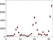
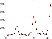
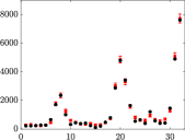
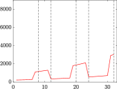
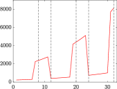
(b) Global factor $\kappa_{t}$ with harmonic specification

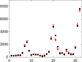
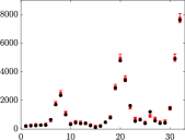
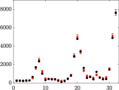
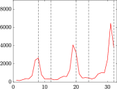
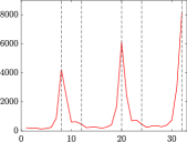
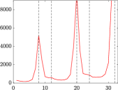
Figure 9: Fire intensity for the harmonic component (panel a) and the dummy variable (panel b) specifications. In each panel, the global number of fires $N_{t}^{y}$ (top,$\bullet$), estimated global fire intensity $\Lambda_{t}(\mathbb{Y})$ (top, $\square$) and the global factor $\kappa_{t}$ (bottom) at a monthly frequency from February 2018 to September 2020. Dashed vertical lines denote the start and end of the dry season (August-December).

$g=0.5^{\circ}$	$g=1^{\circ}$
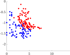
$g=1.5^{\circ}$	$g=2^{\circ}$
$g=2.5^{\circ}$	$g=3^{\circ}$
$g=3.5^{\circ}$	$g=4^{\circ}$

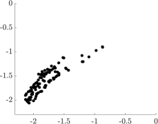
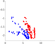
Figure 10: Variability of the intensity estimates, measured by the normalised interquantile range, $(Q_{97.5}-Q_{2.5})/Q_{50}$, for 100 different $g\times g$ areas ($\bullet$). Left: Dry season against wet season range. Right: range against the number of fires in the same areas during dry ($\bullet$) and wet ($\bullet$) seasons.

	Constant scale	Time-varying Scale
$t=3$ (March) $h=0$
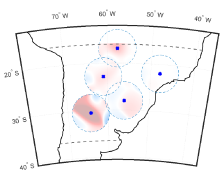
$t=3$ (March) $h=1$
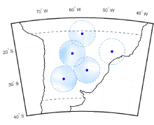
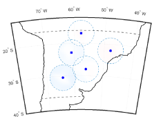
$t=11$ (November) $h=0$
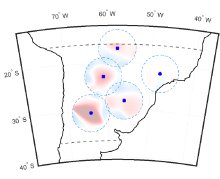
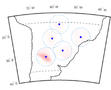
$t=11$ (November) $h=1$

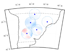
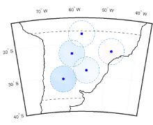
Figure 11: Pair correlation function $\mathscr{R}_{t,t+h}(x,y)$ for harmonic components models with constant (left) and time-varying (right) scale. In each plot, the function value (colours) for $t=3$ (March) and $t=11$ (November) at reference location (dots) $x\in\{(30.521^{\circ}S,64.333^{\circ}W)$, $(22.833^{\circ}S,61.042^{\circ}W)$, $(16.854^{\circ}S,57.750^{\circ}W)$, $(27.958^{\circ}S,56.104^{\circ}W)$, $(21.979^{\circ}S,47.875^{\circ}W)\}$ and alternative locations in a $4^{\circ}$ degree radius around $x$ (circles). Red shades for $\mathscr{R}_{t,t+h}(x,y)>1$ and blue shades for $\mathscr{R}_{t,t+h}(x,y)\leq 1$.

References

- Andrieu et al., (2010) Andrieu, C., Doucet, A., and Holenstein, R. (2010). Particle Markov chain Monte Carlo methods. Journal of the Royal Statistical Society: Series B (Statistical Methodology), 72(3):269–342.
- Andrieu and Thoms, (2008) Andrieu, C. and Thoms, J. (2008). A tutorial on adaptive MCMC. Statistics and Computing, 18(4):343–373.
- Atchadé and Rosenthal, (2005) Atchadé, Y. F. and Rosenthal, J. S. (2005). On adaptive Markov chain Monte Carlo algorithms. Bernoulli, 11(5):815–828.
- Baddeley, (2013) Baddeley, A. (2013). Spatial point patterns: Models and statistics. In Stochastic geometry, spatial statistics and random fields: Asymptotic methods, pages 49–114. Springer.
- Balch et al., (2020) Balch, J. K., St. Denis, L. A., Mahood, A. L., Mietkiewicz, N. P., Williams, T. M., McGlinchy, J., and Cook, M. C. (2020). Fired (fire events delineation): An open, flexible algorithm and database of us fire events derived from the modis burned area product (2001–2019). Remote Sensing, 12(21).
- Bassan and Bona, (1990) Bassan, B. and Bona, E. (1990). Moments of stochastic processes governed by Poisson random measures. Commentationes Mathematicae Universitatis Carolinae, 31(2):337–343.
- Brix, (1999) Brix, A. (1999). Generalized gamma measures and shot-noise Cox processes. Advances in Applied Probability, 31(4):929–953.
- Brix and Diggle, (2001) Brix, A. and Diggle, P. J. (2001). Spatiotemporal prediction for log-Gaussian Cox processes. Journal of the Royal Statistical Society: Series B (Statistical Methodology), 63(4):823–841.
- Brix and Møller, (2001) Brix, A. and Møller, J. (2001). Space-time multi type log Gaussian Cox processes with a view to modelling weeds. Scandinavian Journal of Statistics, 28(3):471–488.
- Chopin et al., (2013) Chopin, N., Jacob, P. E., and Papaspiliopoulos, O. (2013). SMC2: An efficient algorithm for sequential analysis of state space models. Journal of the Royal Statistical Society: Series B (Statistical Methodology), 75(3):397–426.
- Cox, (1955) Cox, D. R. (1955). Some statistical methods connected with series of events. Journal of the Royal Statistical Society: Series B (Methodological), 17(2):129–157.
- Csiszar, (2007) Csiszar, T. L. I. (2007). Reconstruction of fire spread within wildland fire events in Northern Eurasia from the MODIS active fire product. Global and Planetary Change, 56.
- Daley and Vere-Jones, (2008) Daley, D. J. and Vere-Jones, D. (2008). An introduction to the theory of point processes, volume II. General Theory and Structure. Springer.
- Diggle et al., (2013) Diggle, P. J., Moraga, P., Rowlingson, B., and Taylor, B. M. (2013). Spatial and Spatio-Temporal Log-Gaussian Cox Processes: Extending the Geostatistical Paradigm. Statistical Science, 28(4):542 – 563.
- Gerber and Chopin, (2015) Gerber, M. and Chopin, N. (2015). Sequential quasi Monte Carlo. Journal of the Royal Statistical Society: Series B (Statistical Methodology), 77(3):509–579.
- Giglio et al., (2003) Giglio, L., Descloitres, J., Justice, C. O., and Kaufman, Y. J. (2003). An enhanced contextual fire detection algorithm for MODIS. Remote Sensing of Environment, 87(2):273–282.
- Giglio et al., (2016) Giglio, L., Schroeder, W., and Justice, C. O. (2016). The collection 6 MODIS active fire detection algorithm and fire products. Remote Sensing of Environment, 178:31–41.
- Gneiting and Guttorp, (2010) Gneiting, T. and Guttorp, P. (2010). Continuous parameter spatio-temporal processes. In Gelfand, A. E., Diggle, P., Guttorp, P., and Fuentes, M., editors, Handbook of Spatial Statistics, pages 427–436. CRC press.
- Goldman and Singh, (2021) Goldman, J. V. and Singh, S. S. (2021). Spatiotemporal blocking of the bouncy particle sampler for efficient inference in state-space models. Statistics and Computing, 31(5):68.
- Gouriéroux and Jasiak, (2006) Gouriéroux, C. and Jasiak, J. (2006). Autoregressive gamma processes. Journal of Forecasting, 25(2):129–152.
- Hantson et al., (2016) Hantson, S., Arneth, A., Harrison, S. P., Kelley, D. I., Prentice, I. C., Rabin, S. S., Archibald, S., Mouillot, F., Arnold, S. R., Artaxo, P., Bachelet, D., Ciais, P., Forrest, M., Friedlingstein, P., Hickler, T., Kaplan, J. O., Kloster, S., Knorr, W., Lasslop, G., Li, F., Mangeon, S., Melton, J. R., Meyn, A., Sitch, S., Spessa, A., van der Werf, G. R., Voulgarakis, A., and Yue, C. (2016). The status and challenge of global fire modelling. Biogeosciences, 13(11):3359–3375.
- Jalilian et al., (2015) Jalilian, A., Guan, Y., Mateu, J., and Waagepetersen, R. (2015). Multivariate product-shot-noise Cox point process models. Biometrics, 71(4):1022–1033.
- Jones et al., (2022) Jones, M. W., Abatzoglou, J. T., Veraverbeke, S., Andela, N., Lasslop, G., Forkel, M., Smith, A. J. P., Burton, C., Betts, R. A., van der Werf, G. R., Sitch, S., Canadell, J. G., Santín, C., Kolden, C., Doerr, S. H., and Le Quéré, C. (2022). Global and regional trends and drivers of fire under climate change. Reviews of Geophysics, 60(3):e2020RG000726.
- Kantas et al., (2015) Kantas, N., Doucet, A., Singh, S. S., Maciejowski, J., and Chopin, N. (2015). On particle methods for parameter estimation in state-space models. Statistical Science, 30(3):328–351.
- King et al., (2021) King, G. K. K., Papaspiliopoulos, O., and Ruggiero, M. (2021). Exact inference for a class of hidden Markov models on general state spaces. Electronic Journal of Statistics, 15(1):2832 – 2875.
- Last and Penrose, (2018) Last, G. and Penrose, M. (2018). Lectures on the Poisson process. Cambridge University Press.
- Møller, (2003) Møller, J. (2003). Shot noise Cox processes. Advances in Applied Probability, 35(3):614–640.
- Møller and Díaz-Avalos, (2010) Møller, J. and Díaz-Avalos, C. (2010). Structured spatio-temporal shot-noise Cox point process models, with a view to modelling forest fires. Scandinavian Journal of Statistics, 37(1):2–25.
- Møller et al., (1998) Møller, J., Syversveen, A. R., and Waagepetersen, R. P. (1998). Log Gaussian Cox processes. Scandinavian Journal of Statistics, 25(3):451–482.
- Møller and Waagepetersen, (2003) Møller, J. and Waagepetersen, R. P. (2003). Statistical inference and simulation for spatial point processes. CRC press.
- Monfort et al., (2017) Monfort, A., Pegoraro, F., Renne, J.-P., and Roussellet, G. (2017). Staying at zero with affine processes: An application to term structure modelling. Journal of Econometrics, 201(2):348–366.
- Naik et al., (2022) Naik, C., Caron, F., Rousseau, J., Teh, Y. W., and Palla, K. (2022). Bayesian nonparametrics for sparse dynamic networks. In Joint European Conference on Machine Learning and Knowledge Discovery in Databases, pages 191–206. Springer.
- Papaspiliopoulos et al., (2016) Papaspiliopoulos, O., Ruggiero, M., and Spanò, D. (2016). Conjugacy properties of time-evolving Dirichlet and gamma random measures. Electronic Journal of Statistics, 10(2):3452 – 3489.
- Pitt and Walker, (2005) Pitt, M. K. and Walker, S. G. (2005). Constructing stationary time series models using auxiliary variables with applications. Journal of the American Statistical Association, 100(470):554–564.
- Pontes-Lopes et al., (2021) Pontes-Lopes, A., Silva, C. V., Barlow, J., Rincón, L. M., Campanharo, W. A., Nunes, C. A., de Almeida, C. T., Silva Júnior, C. H., Cassol, H. L., and Dalagnol, R. (2021). Drought-driven wildfire impacts on structure and dynamics in a wet Central Amazonian forest. Proceedings of the Royal Society B, 288(1951):20210094.
- Raftery et al., (2017) Raftery, A. E., Zimmer, A., Frierson, D. M., Startz, R., and Liu, P. (2017). Less than 2 c warming by 2100 unlikely. Nature Climate Change, 7(9):637–641.
- Richardson et al., (2020) Richardson, R., Kottas, A., and Sansó, B. (2020). Spatiotemporal modelling using integro-difference equations with bivariate stable kernels. Journal of the Royal Statistical Society: Series B (Statistical Methodology), 82(5):1371–1392.
- Sim, (1990) Sim, C. H. (1990). First-order autoregressive models for gamma and exponential processes. Journal of Applied Probability, 27(2):325–332.
- Singh et al., (2017) Singh, S. S., Lindsten, F., and Moulines, E. (2017). Blocking strategies and stability of particle Gibbs samplers. Biometrika, 104(4):953–969.
- Taylor and Diggle, (2014) Taylor, B. M. and Diggle, P. J. (2014). INLA or MCMC? A tutorial and comparative evaluation for spatial prediction in log-Gaussian Cox processes. Journal of Statistical Computation and Simulation, 84(10):2266–2284.
- Tyukavina et al., (2022) Tyukavina, A., Potapov, P., Hansen, M. C., Pickens, A. H., Stehman, S. V., Turubanova, S., Parker, D., Zalles, V., Lima, A., Kommareddy, I., Song, X., Wang, L., and Harris, N. (2022). Global trends of forest loss due to fire from 2001 to 2019. Frontiers in Remote Sensing, 3:825190.
- Waagepetersen et al., (2016) Waagepetersen, R., Guan, Y., Jalilian, A., and Mateu, J. (2016). Analysis of multispecies point patterns by using multivariate log-Gaussian Cox processes. Journal of the Royal Statistical Society: Series C (Applied Statistics), 65(1):77–96.
- Wolpert and Ickstadt, (1998) Wolpert, R. L. and Ickstadt, K. (1998). Poisson/gamma random field models for spatial statistics. Biometrika, 85(2):251–267.
Supplementary Material for “A Spatiotemporal Gamma Shot Noise Cox Process”