Label Propagation Techniques for Artifact Detection in Imbalanced Classes using Photoplethysmogram Signals

Abstract

This study aimed to investigate the application of label propagation techniques to propagate labels among photoplethysmogram (PPG) signals, particularly in imbalanced class scenarios and limited data availability scenarios, where clean PPG samples are significantly outnumbered by artifact-contaminated samples. Our research compares the performance of supervised classifiers, such as conventional classifiers and neural networks (Multi-Layer Perceptron (MLP), Transformers, Fully Convolutional Network (FCN)), with the semi-supervised label propagation algorithm for artifact classification in PPG signals. The results indicate that the label propagation algorithm achieves a precision of 91%, a recall of 90%, and an F1 score of 90% for the ”artifacts” class, showcasing its effectiveness in annotating a medical dataset, even in cases where clean samples are rare. Although the K-Nearest Neighbors (KNN) supervised model demonstrated good results with a precision of 89%, a recall of 95%, and an F1 score of 92%, the semi-supervised algorithm excels in artifact detection. In the case of imbalanced and limited pediatric intensive care environment data, the semi-supervised label propagation algorithm is promising for artifact detection in PPG signals. The results of this study are important for improving the accuracy of PPG-based health monitoring, particularly in situations in which motion artifacts pose challenges to data interpretation.

=-21pt

I Introduction

Machine learning, a sub-field of artificial intelligence [1], has emerged as a transformative technology in various domains, including healthcare. With its ability to analyze large amounts of data [2] and find important patterns, machine learning is a robust technique. It has the potential to improve healthcare outcomes, help doctors make better decisions [3], and revolutionize medical research. Using advanced algorithms and computing power, machine learning can extract all the necessary information from various types of healthcare data, such as electronic medical records [4], medical images, and physiological signals.

In clinical context, machine learning techniques can improve decision making. Support systems help with things like medication alerts and reminders for patient safety. Indeed, the model uses patient medical records and the vast amount of information available to develop models that aim to predict injuries [5], detect heart disease earlier [6] and mortality [7]. Based on clinical experience and physiological principles, machine learning provides scores that enable hospital staff to make faster, more accurate decisions. Additionally, machine learning algorithms can contribute to drug discovery and development by expediting the identification of promising drug targets, optimizing drug efficacy, and predicting potential adverse reactions [8].

Despite its potential, the integration of machine learning into healthcare comes with challenges and considerations. Privacy and ethical implications must be taken into account when applying machine learning to healthcare [9]. The data acquired must respect patient privacy and confidentiality. This data is often recorded by several devices, so it is important to link the recordings so that the data is standardized and can be more easily managed. In order to be able to link these data, they need to be collected in a single database, and thus be consistent with each other. In other words, the data must be harmonized [10]. Data security and accountability should be prioritized, especially when using cloud-based technologies that require extensive storage and computing power.

One major concern is the availability of high-quality data for training and testing these algorithms [11]. To be able to evaluate the performance of the algorithms implemented, it is necessary to have access to a ground truth. This ground truth is often non-existent or requires the help of experts, and is often time-consuming. Moreover, it’s crucial to have a large enough sample size to ensure accurate and reliable predictions. However, obtaining such labeled data can be challenging, as it may be limited and incomplete. Furthermore, the imbalance in classes during the algorithm’s training phase is a common consequence of medical data predominantly representing the most frequent cases present in patients. Consequently, a significant challenge arises in rebalancing the data whereas ensuring the retention of its crucial medical value. Additionally, the amount of erroneous, missing or imprecise data is an obstacle to model prediction. Erroneous data are data which have been altered by abnormal occurrences. Continuous waveform data captured by sensors is vulnerable to high-frequency artifacts that often result from patient motion or clinical interventions. Even periodic clinical measurements are not immune to contamination, as data collection and coding practices can introduce issues [10].

The main objective of this work is to detect motion artifacts in photoplethysmogram (PPG) signals obtained from the pediatric intensive care unit (PICU) database of the CHU Sainte-Justine hospital (CHUSJ). PPG signals are frequently captured during different types of movements which introduces motion noise and interferes with the accuracy of the signals. This noise is irregular and causes high-amplitude fluctuations within the PPG signals [12]. Motion artifacts can result in the pulse oximeter either misinterpreting movement as the actual signal or masking the true signal with unwanted interference, which can lead to incorrect readings, false alarms, and missed important alarms [13]. The cleaned PPG signals will be used in the construction of clinical decision systems (CDSS) at the PICU of CHUSJ. Specifically, annotated signals will be used in screening and identifying various health-related concerns on children. As an example, changes in blood pressure in children serve as significant indicators for identifying patients who require immediate care and admission to the PICU. Invasive methods, like catheter insertion for continuous blood pressure monitoring, offer precise real-time data but come with significant risks such as bleeding and infection [14]. On the other hand, conventional cuff-based measurements, though less invasive, provide only intermittent readings and may not capture sudden clinical changes effectively. Therefore, predicting blood pressure from PPG waveforms has emerged as a successful approach [15] for comprehensive CDSS applications. In this project, we used a semi-supervised labeling algorithm to annotate PPG signals to effectively remove artifacts from them in real-time. A small proportion of data was annotated by an expert and a statistical analysis algorithm was then used to validate the annotations. To annotate the entire dataset, a machine learning algorithm that annotates all data using only a small proportion of previously annotated data, was used. The Label Propagation (LP) algorithm is a machine learning technique used for semi-supervised learning tasks. This algorithm is effective in our scenario because the availability of labeled data is limited and there is a large amount of unlabeled data [16].

Our medical data are very unbalanced, with around 80% of pulses free of artifacts and only 20% with artifacts. This means that to have an accurate labeling algorithm, a rebalancing of the classes in the training part need to be done. Several methods are available for this: oversampling, undersampling and, both oversampling and undersampling. It must be remembered that medical data is being worked with, so using sampling methods must make medical sense, whether by randomly duplicating data or by removing it. Medical data involves intricate relationships among different data elements, such as patient demographics, medical history, symptoms, diagnoses, treatments, and outcomes [17].

Another aim of this project is to compare classifiers to the Label Propagation algorithm, used as a classifier, to accurately detect artifacts. In [18] the authors explore the use of semi-supervised models to classify temporal data. These models are based on a graphical approach, such as the label propagation algorithm. The results of the algorithm are evaluated on different datasets of varying lengths, including ECG (electrocardiogram) signal data. The results show that semi-supervised models are accurate for classifying time series data. However, these algorithms have not been applied to artifact detection. Semi-supervised learning is widely used as a classification algorithm in cases where not all data is annotated. Active learning is also a very powerful semi-supervised classification method that has proven its effectiveness for temporal data [19].

Machine learning classifiers are designed to categorize data into distinct classes or groups based on specific features or patterns. The use of classifiers has witnessed significant growth across different domains, especially in health care, where classifiers are a real help in decision-making [20]. By leveraging statistical analysis and optimization techniques, classifiers enable accurate predictions and information retrieval. The spectrum of classifiers is very wide: from traditional classifiers like K-Nearest Neighbors (KNN), Support Vector Machine (SVM), Decision Tree (DT), Naive Bayes classifier (NB) [21], to classifiers using neural networks, such as Multi-Layer Perceptron classifier (MLP) or Transformers. A comparison of the results of each type of classifier with the semi-supervised Label Propagation algorithm will be dressed. The effectiveness of these two streams is analyzed by the experimental results (in section IV) from the comparative analysis of semi-supervised label propagation (label propagation with KNN kernel) and fully-supervised learning, including conventional machine learning classifiers (KNN, Support Vector Classification (SVC), DT, Random Forest (RF), GaussianNB, MultinominalNB, and Logistic Regression (LR)), MLP, and Transformers. Then, the best classification method will be presented, followed by a conclusion on artifact detection.

The paper is structured as follows. In section II, data characteristics, preprocessing and methodology: labeling and classification, are introduced. In section III, the implementation of experiments is presented. Section IV is used to evaluate the results with different metrics and present a comparison of experimental result tables. In section V, the results are interpreted and the limitations are discussed.

II Material and Methods

This study was conducted following ethical approval from the research ethics board at CHUSJ (protocol number 2023-4556, accepted January 18, 2023). The detailed workflow of the various work stages is shown in the Fig. 1.

II-A Data Collection

The aim of this project is to detect motion artifacts in PPG signals. The eligible study population includes all children aged 0 to 18 years, admitted between September 2018 and July 2022 inclusive, for whom electrocardiogram (ECG), PPG and arterial blood pressure (ABP) waveform records are available. In this population, specific exclusion criteria have been established to avoid bias. Data collected beyond the fourth day of hospital stay will be disregarded to prevent potential bias from a few patients who may have prolonged stays with arterial lines. Patients on extracorporeal membrane oxygenation (ECMO) treatment will also be excluded from the analysis. Furthermore, if a patient is readmitted to the PICU multiple times, only data from the first stay will be considered for analysis.

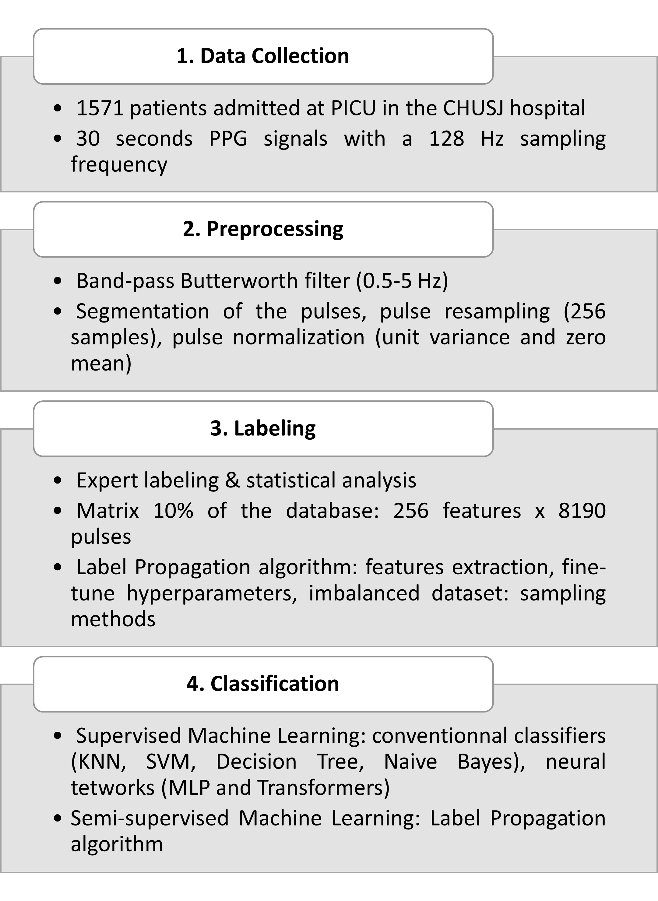
Figure 1: Workflow of the proposed method for detecting motion artifacts in PPG signals.

A PPG signal is recorded using a sensor called the pulse oximeter. This device is placed on a patient’s skin, for children on a fingertip or earlobe. A PPG sensor emits light into the skin, which is partially absorbed by the blood vessels. Changes in blood flow during the cardiac cycle cause variations in light absorption. The sensor detects the reflected light, measuring its intensity modulated by blood volume changes. This varying intensity is converted into an electrical signal, creating the PPG waveform. Blood pressure signals are recorded using an invasive and continuous method, i.e., the catheter, and a non-invasive and discontinuous method, i.e., the blood pressure cuff. ECG is continuously recorded by placing electrodes on the patient’s chest. The Sainte-Justine University Hospital Pediatric Intensive Care Unit (PICU) utilizes a high-resolution research database (HRDB) [22, 23] that has been approved by the ethical committee. The HRDB links biomedical signals extracted from the different devices, displayed through patient monitors, to the electronic patient record continuously throughout their stay in the unit [24].

Between 2018 and 2022, 1571 patients met the inclusion criteria. For each patient, four physiological signals were extracted: ECG, PPG, blood pressure from the catheter, and blood pressure from the cuff. Each signal was extracted over a period of 96 hours (4 days). Signal values are grouped together in a table with the date and time of acquisition. For the PPG signal, 640 values are acquired every 5 seconds, corresponding to a sampling frequency of 128 Hz. For blood pressure and ECG signals, 2560 values are acquired every 5 seconds, with a sampling frequency of 512 Hz. For the duration of the extraction, a fixed 30-second window of PPG signals will be used for the further processing.

II-B Preprocessing

The raw PPG signal is preprocessed to increase its quality, remove unwanted noise, and make it more suitable for subsequent processing steps [25]. The different steps are described below:

1. Filtering: each signal window is filtered using a band-pass Butterworth filter, the cut-off frequencies are 0.5 and 5 Hz, corresponding to a heart rate between 30 and 300 bpm. A forward-backward filtering is used to avoid phase distortions. The objective is to remove baseline wander and high-frequency noise.

2. Pulse segmentation: a function to finds all local minima by a comparison between samples is used. The aim is to divide the preprocessed PPG signal into smaller segments or windows to be able to detect the artifacts present for each pulse. In our case, a segment is a pulse. The size of each segment may vary depending on the characteristics of the PPG signal and the specific application the signal pulses. A pulse is considered to lie between two minima.

3. Resampling: the duration of a cardiac cycle for children is between 0.3 and 1 second. A pulse is representing a cardiac cycle. Therefore, not all pulses have the same number of samples. Each pulse is uniformly oversampled in time to contain 256 samples, which corresponds to a heart cycle of 1s. A linear interpolation function [26] is used to create the missing points for each pulse. Linear interpolation is favored for signals due to its simplicity, computational efficiency, and ability to estimate values between known data points. It maintains signal continuity and linearity, making it suitable for signals with relatively smooth and linear variations.

4. Normalization: the data are normalized to have a unit variance and zero mean. This normalization ensures that all features or variables in the data have the same scale, preventing certain features from dominating the learning process simply because they have larger numerical values.

5. Data transformation: each PPG pulse, which is essentially a waveform representing blood volume changes over time, can be represented as a data point in a column that contains 256 values. These values are equally spaced points obtained using step 3 of the preprocessing. At the end of preprocessing, a vector of 256 points is obtained, representing a pulse of the PPG signal. The number of vectors depends on the number of pulses. This method allows to work with PPG data in a structured manner, suitable for a range of applications, from statistical analysis to machine learning.

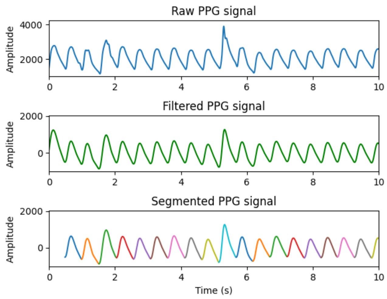
Figure 2: Example of a 10s segment of a 30s raw PPG signal in the top image, filtered signal in the middle image and segmented signal in the bottom image.

The Fig. 2 shows the first 10 seconds of a raw PPG signal, then when the signal has been filtered and finally when the pulses have been segmented. The effect of the bandpass filter can be seen in the second figure. The filter has smoothed the signal by removing the extreme frequency components. The signal waveform is preserved, and the filter does not introduce resonances or significant ripples in the desired frequency range. Note that the first pulse has not been segmented. This is because the function could not detect the two minima that make up a pulse and therefore could not segment it. The signal does not start at the first low point of the pulse.

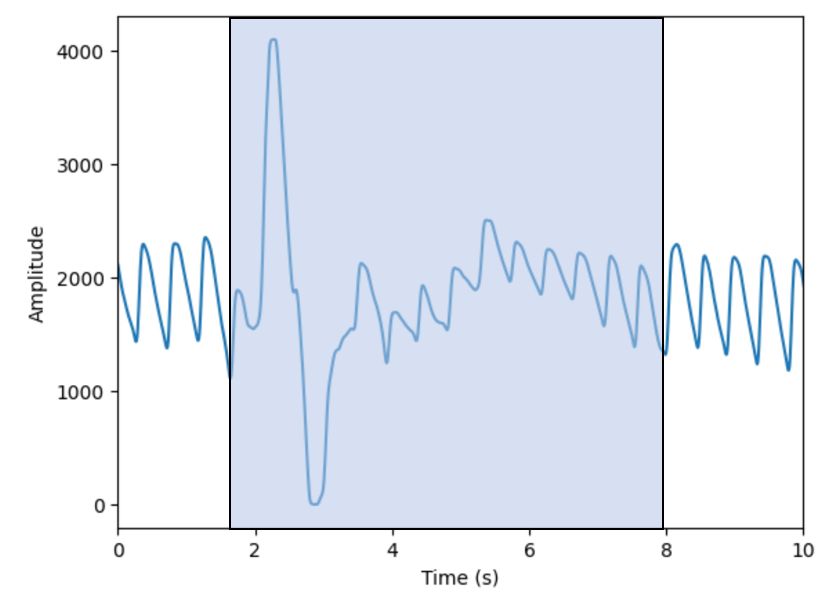
Figure 3: Example of a 10s segment of a 30s raw PPG signal. Inside the blue box are all the pulses containing motion artifacts.

II-C Dataset annotation

First, after preprocessing the data, the aim is to build a ground truth for future evaluation of the classification algorithms. In this objective, one human expert annotated 10% of the database. Annotation is visual, comparing pulses with each other and binary classifying each pulse as good or as containing artifacts. To avoid involving another human expert, in consideration of time and specialist resources, we implemented an automated algorithm to handle additional annotations. This algorithm, acting as a surrogate expert, was developed to recheck the entirety of the 10% annotated data by the human expert, identifying similarities in the process. Employing a statistical approach, the algorithm determines if the values of a given pulse lie within standard parameters or deviate from the norm. We subsequently cross-validated the algorithm’s annotations against those from the professional expert to determine the algorithm’s accuracy. It was decided to annotate a maximum of 10% of the database and then use the label propagation algorithm to annotate the rest of the data.

II-C1 Expert labeling

PPG signals already segmented are presented to the expert. By analyzing each pulse, the expert classifies each pulse as artifact or artifact-free. A pulse is defined as artifact-free if its morphology is typical i.e. if its characteristics - amplitude, width, shape - are the same as those of adjacent signals. A pulse is defined with artifacts if its characteristics differ from those of adjacent pulses (see Fig. 3). To recheck the annotations of one expert, an algorithm that acts as a second expert was set up, allowing all impulses to be reannotated to see similarities. This algorithm uses a statistical approach to assess whether the statistical values of a pulse are normal or outside the norm.

II-C2 Statistical analysis

For each cardiac cycle, which corresponds to a pulse, if the waveform is similar, statistics such as skewness, standard deviation (std) and kurtosis are approximately constant for each cycle. It is therefore possible to detect motion artifacts by using the value of these statistics to differentiate a pulse without artifacts from a pulse with motion artifacts [27]. Skewness indicates the degree of asymmetry in the probability distribution of a random variable around its mean. It can take on positive, zero, negative, or undefined values, reflecting the shape and symmetry of the distribution. Kurtosis is the sharpennes of the peak of a frequency-distribution curve and standard deviation reflects the dispersion degree of a data set. If $X$ is considered a variable with $\mu$ and $\sigma$ the mean and standard deviation respectively, statistical values are calculated as follows:

$$\text{Kurt}[X]=E\left[\left(\frac{X-\mu}{\sigma}\right)^{4}\right]=\frac{E\left[\left(X-\mu\right)^{4}\right]}{\sigma^{4}}$$ (1)

$$\text{Skew}[X]=E\left[\left(\frac{X-\mu}{\sigma}\right)^{3}\right]=\frac{E\left[\left(X-\mu\right)^{3}\right]}{\sigma^{3}}$$ (2)

$$\text{std}[X]=\sqrt{E\left[\left(X-\mu\right)^{2}\right]}$$ (3)

These values are calculated for each pulse of a signal. So in our case, the variable X represents a vector of all the samples in a pulse. If the shape of the cycle changes, then these statistical values will no longer be constant. To be able to detect outliers, thresholds that detect skewness, kurtosis and standard deviation values that are not normal, i.e. values for artifact-free cycles, were set up. For this reason, the distribution of each of these three statistics over a pulse can be estimated using a normal distribution [28]. The aim is to reduce the risk of a pulse being incorrectly annotated. To do this, a wide confidence interval is taken to ensure that the probability that the value of the corresponding statistic is not unnecessarily rejected. If X is considered to be a variable which can be approximated by a normal distribution $\mathcal{N}(\mu,\,\sigma^{2})$, the probability that this variable lies within the chosen confidence interval can be written as follows:

$$\mathbb{P}(\mu-2\sigma\leq X\leq\mu+2\sigma)\approx 0.9545$$ (4)

After several experiments, this 95% confidence interval gives the best results, as it reduces the risk of poor detection. So a lower and an upper thresholds can be defined as follows:

$$th_{l}=\mu-2\sigma$$ (5)

$$th_{u}=\mu+2\sigma$$ (6)

With the mean and standard deviation calculated for each statistic measure by taking the set of values for each pulse of a signal. To effectively detect motion artifacts, a waveform segment is classified as containing motion artifacts if at least one of the three statistics falls outside the defined thresholds. The result of this first step is a small proportion of the annotated dataset, with a binary value for each pulse: pulse with artifact or without artifact. The annotations given by the algorithm are then compared with the expert’s annotations and found to have 80% similarity. After examining the annotations with the expert, the function chosen to segment the pulses did not always correctly segment a pulse that was formed by a distinct diastole and systole curve. In a cardiac cycle, diastole is the relaxation phase when the heart fills with blood, and systole is the contraction phase when the heart pumps blood out to the body or lungs. In this case, two pulses were detected instead of one. This segmentation error partly explains the 20% difference in annotation between the expert and the algorithm. The percentage of similarity is considered high enough to validate the expert’s annotations.

II-C3 Imbalanced dataset

The two classes of annotated data are unevenly distributed. In fact, the annotation includes many more pulses without motion artifacts, approximately 80% and 20% of pulses with motion artifacts. For accurate results with the algorithms, the data needs to be resampled. The complex characteristics of our clinical data: small training size, many features, and correlations between the features, makes the task more complicated. Understanding the interconnectedness of these variables is crucial for accurate analysis and prediction [17]. Oversampling and undersampling methods are the most frequently used. Under-sampling reduces the majority class examples, achieving a balanced dataset, with random under-sampling (RUS) being a well-known method. However, under-sampling may lead to the loss of valuable information from the majority class. On the other hand, over-sampling increases the minority class examples. Random over-sampling (ROS) replicates existing minority examples, but it may result in overfitting. Synthetic minority over-sampling technique (SMOTE) generates artificial minority examples by interpolating between selected examples and their nearest neighbors. Modifications such as adaptive synthetic sampling (ADASYN) adjust the number of artificial minority examples based on the density of majority examples surrounding the original minority example [29]. Also, it is concluded that there is no clear winner between oversampling and undersampling to compensate for the class imbalance if factors such as class distribution, class prevalence, and features correlations in medical decision-making [17] are not taken into consideration. In the section IV the different results obtained with the sampling methods will be presented, to conclude on the best method for our study.

II-C4 Label Propagation

The Label Propagation algorithm is an iterative algorithm that assigns labels to unlabeled data points by propagating labels through the dataset [30]. In graph-based semi-supervised learning methods, a graph where each node is represented by a vector of features is created. The edges between nodes are weighted based on how similar the features are. When the weights of the edges are high, it means that the connected nodes are likely to have the same label. This idea is based on the assumption that samples close to each other in the graph are part of the same group or category [31]. At the start of the algorithm, only a small proportion of the data is already labeled, corresponding here to the proportion of data annotated in the previous step. In our case, considering that we have around 51 pulses per signal and that we have annotated 10% of the entire database of 1571 signals, we therefore have 8000 pulses, and thus 8000 nodes in the graph. This algorithm is based on the hypothesis that if two nodes are connected that means they carry a similarity. Usually, the Euclidean distance between nodes is calculated to establish the graph. Depending on the kernels chosen for the algorithm’s operation, this distance measurement may be different. Consider the following notations:

$$u :\text{number of unlabeled points}$$

$$l :\text{number of labeled points}$$

$$k :\text{number of classes}$$

The aim of this algorithm is to look, in the final state, at all the probabilities a node has of belonging to a certain class and to take the largest. $Y$ a matrix with rows containing the probabilities that a node belongs to a certain class is considered. This matrix $Y$ is a $N\times k$ matrix where $N=l+u$. Also considered $T$, a $N\times N$ probability transition matrix. This matrix T is obtained by calculating the degree matrix ($D$) and the adjacency matrix ($A$). It defines the probability of jumping from one node to another in $t$ steps. This number $t$ can tend towards infinity [32]. The matrix $Y$ contains two sub-matrices: $Y_{l}$ and $Y_{u}$, respectively for the known and unknown labels. The same applies to the $T$ matrix, which contains 4 sub-matrices:

• $T_{ll}$: probability to get from labelled nodes to labelled nodes. This matrix will be an identity matrix.

• $T_{lu}$: probability to get from labelled nodes to unlabelled nodes. This will be a zero matrix because labelled nodes are absorbing states, it means you are in a self-loop and can’t move in any direction.

• $T_{ul}$ and $T_{uu}$: probability to get from unlabelled nodes to labelled and unlabelled nodes respectively.

Consider $\hat{Y}$, the probability matrix of annotations obtained in the final state. The matrix T is set to the infinite power and $Y_{0}$ represents the initial annotations of the nodes. The equation for the final state of this algorithm can be expressed as:

$$\hat{Y}=T^{t\rightarrow\infty}Y_{0}$$ (7)

In 7, the matrix $T$ is set to the power $t$ with $t$ tending to infinity. It can be written:

$$\lim\limits_{t\to\infty}T^{t}=\begin{bmatrix}I&0\\ \left(\sum_{t=0}^{\infty}T_{uu}^{t}\right)T_{ul}&T_{uu}^{\infty}\end{bmatrix}$$ (8)

The sum between the brackets is similar, when $t$ tends to infinity, to a geometric series that has an argument that is less than 1 in modulus. And if $T_{uu}$ is multiplied by itself a large number of times, knowing that the values are less than 1, it will become very close to 0. Therefore, a conclusion on the limit of the transition matrix for a very large number of steps, is:

$$\lim\limits_{t\to\infty}T^{t}=\begin{bmatrix}I&0\\ \left(I-T_{uu}\right)^{-1}T_{ul}&0\end{bmatrix}$$ (9)

The equation 7 can, therefore, be rewritten:

$$\begin{bmatrix}\hat{Y_{l}}\\ \hat{Y_{u}}\end{bmatrix}=\begin{bmatrix}I&0\\ \left(I-T_{uu}\right)^{-1}T_{ul}&0\end{bmatrix}\begin{bmatrix}Y_{l0}\\ Y_{u0}\end{bmatrix}$$ (10)

For unknown labels, the following formula can be written:

$$\hat{Y_{u}}=\left(I-T_{uu}\right)^{-1}T_{ul}Y_{l0}$$ (11)

This matrix contains the new labels and is the output of the algorithm. To sum up, the various stages of the algorithm can be summarized as follows:

1. Creation of a graph with nodes labeled and unlabeled.

2. Calculation of the probability transition matrix $T$. This matrix is linked to the degree matrix $D$, it is a diagonal matrix where each diagonal element corresponds to the sum of edge weights connected to that node. And also linked to the adjacency matrix $A$, it is a square matrix where each row and column corresponds to a node, and the value at the intersection indicates whether there’s an edge (value 1, otherwise 0) connecting those nodes. The formula is: $T=D^{-1}\cdot A$. This matrix is the same throughout the algorithm.

3. Calculation of the new labels for each $t$ iteration:

   $$Y^{t+1}=T^{t}Y^{t}$$ (12)

4. Repeat step 3 until convergence.

While performing label propagation, groups of closely linked nodes quickly reach a consensus on a single label, causing many labels to vanish. This leaves only a few labels remaining after propagation. When nodes end up with the same label after convergence, it signifies that they are part of the same group.

II-D Classification

Once the ground truth has been established, the aim is to classify the pulses and compare the results obtained with the annotations. Machine learning classifiers are used for classification. These automatic algorithms categorize data into the two classes of our problem. They operate as mathematical models, utilizing statistical analysis and optimization techniques to detect patterns within the data. By identifying these patterns, classifiers can assign each instance to a specific class or category. There are a wide variety of traditional classifiers, both supervised and unsupervised. To process medical data, which is also temporal data, supervised classifiers have been chosen to be utilized. Here are 4 examples [21]:

1. K-Nearest Neighbor (KNN): this is a supervised method where k represents the number of neighbors. For classification, when given a new input data point, the algorithm identifies the k nearest neighbors from the training dataset based on their feature similarity. The class label of the majority of these k neighbors is then assigned to the new data point.

2. Support Vector Machine (SVM): in SVM, data points are mapped as vectors within a high-dimensional space. The algorithm aims to identify the optimal hyperplane that distinctly categorizes the classes. In binary classification, a hyperplane can be considered as a boundary delineating two distinct data classes. While numerous hyperplanes might achieve this separation, the algorithm selects the one that provides the most effective separation. For a specific classification purpose, as is the case for this project, we have subsequently used SVC (Support Vector Classification) which is a type of SVM specialized for classifications.

3. Decision Tree: Each internal node represents a feature or attribute, and each branch represents a decision rule based on that feature. The leaf nodes of the tree represent the final class label or predicted value. During training, each value is separated based on the attribute. When making predictions, new data points traverse the decision tree by following the decision rules at each node until reaching a leaf node, which then provides the predicted class label or value.

4. Naive Bayes classifier: this classifier use probability to predict whether an input will fit into a certain category. It builds a statistical model based on these probabilities. Naive Bayes calculates the likelihood of the data point belonging to each class using the previously estimated probabilities.

Traditional classifiers have big advantages for small or medium datasets that require simpler or linear models. They have few layers in their architecture, on the other hand, deep learning (MLP and Transformers) architectures are comprised of multiple layers of neural networks. Deep architectures take advantage of unsupervised pre-training at layer level, which facilitates efficient tuning of the deep networks and enables them to extract intricate structures from input data. These extracted features at higher levels contribute to improved predictions and overall performance [33]. For classification, MLP and Transformers are neural networks classifiers:

• Multilayer Perceptron (MLP): it consists of multiple layers of nodes (neurons) that are interconnected through weighted connections. MLP employs a feedforward mechanism, where information flows from the input layer through the hidden layers to the output layer. Each node in the network applies an activation function to the weighted sum of its inputs to produce an output. Through a process called backpropagation, the MLP classifier adjusts the weights to minimize the error between predicted and actual labels during training.

• Transformers: it relies on the attention mechanism. The attention-mechanism looks at an input sequence and decides at each step which other parts of the sequence are important. Transformer is an architecture for transforming one sequence into another one with the help of two parts (Encoder and Decoder).

The objective is to apply all these classifiers to the PPG signal pulses so that a comparison of the classifiers on our medical data can be built. In addition to being compared with each other, these classifiers will also be compared with the Label Propagation semi-supervised algorithm, which not only annotates our database but also classifies artifacts in PPG signals.

III Experimental Implementation

First, as a reminder, in the Label Propagation algorithm, the two input matrices are the annotation matrix, which is a binary vector, and a matrix containing the features for each pulse. Each pulse represents a node in the algorithm’s graph. For the choice of features, the signal from a temporal perspective has been considered. Therefore, an input matrix for the algorithm of size 256 samples $\times$ the number of pulses, can be obtained.

To be able to evaluate our results different metrics have been chosen. The negative state (0) is a pulse without motion artifacts, whereas the positive state (1) is a pulse with motion artifacts. All these measures are based on the evaluation of false negatives (FN), pulse with artifact incorrectly identified as a clean pulse, false positives (FP), clean pulse incorrectly identified as a pulse with artifact, true negatives (TN), clean pulse correctly identified as a clean pulse, and true positives (TP), pulse with artifact correctly identified as a pulse with artifact. The following metrics are defined:

• Confusion Matrix: a table with two rows and two columns that reports the number of true positives, false negatives, false positives, and true negatives.

• Precision, Recall & F1: these three scores give a more general idea of how the algorithm works, rather than just looking at the algorithm’s accuracy, which can be biased in certain situations. They are defined as follows:

  $$\text{Precision}=\frac{TP}{TP+FP}$$

  $$\text{Recall}=\frac{TP}{TP+FN}$$

  $$\text{F1}=2*\frac{\text{Precision}*\text{Recall}}{\text{Precision}+\text{Recall}}$$

• AUROC: the AUROC (Area Under the Receiver Operating Characteristic curve) represents the probability that the model correctly ranks a randomly chosen positive instance higher than a randomly chosen negative instance. The ROC curve is created by plotting the TP rate against the FP rate.

Using these metrics, the hyperparameters of our model for the Label Propagation algorithm need to be defined. The first parameters defined are the parameters of the function used. The choice of kernel is between KNN or RBF (radial basis function), and depending on this choice, two other associated parameters could be modified. The maximum number of iterations and the algorithm’s convergence tolerance remained the default values: 1000 iterations and $10^{-3}$ for the threshold of convergence. The first parameter to be defined was the choice of kernel. For this, a cross-validation was carried out on the data. This involves dividing the data into several parts, then running the two algorithms using different values for the parameters on each part, keeping one part aside for performance testing. Then a calculation of the average performance can be done over all the test parts for each value and choose the one that gives the best performance. A KNN kernel with a number of neighbors of 7 has been chosen. The data are separated as follows: 70% training and 30% testing. The data from the training part are redivided evenly to obtain 50% of unlabeled data and 50 % of labeled data.

IV Results and Discussion

To optimize the Lable Propagation algorithm to achieve the best performance on automatic labeling, different proportions of the dataset were tried for annotation. The aim is to annotate as few pulses as possible. 2.5%, 5%, 7.5%, and 10% of the dataset were annotated, given that the entire database contains 1571 signals, and the proportion that gave the best results was evaluated. For each proportion of the dataset the precision, recall and F1 values were analyzed to decide. The results for the class 1 (class ”pulse with artifacts”) of these metrics are presented in the table II. Because the data are imbalanced, the results for the class 0 (class ”pulse without artifacts”) remain consistently good and don’t change much with different parameters. The best results are obtained for a proportion of 5% of the dataset. Indeed, as the proportion of annotated data increases, the distribution of classes becomes even more disparate. For 2.5% there are 17.3% of pulses with artifacts, and for 5% the proportion of pulses with artifacts is 18.1%. As the size of the annotated dataset increases, for 7.5% there are 16.4% of pulses with artifacts. For 10% of the dataset, 17.7% of pulses contain artifacts. All these values are summarized in the table I. If the classes are more unbalanced, this may have an influence on the algorithm, which will have greater difficulty in finding a constant pattern for propagating the labels. In the case of 10%, the proportion of pulses with artifacts is high, but the number of annotated pulses increases, and this may induce new data that is less representative of the overall data distribution, leading to poor generalization on unseen data.

TABLE I: Summary table containing the labeling portion and the imbalance rate

Dataset proportion	Artifacts (%)	Non-artifacts (%)
2.5%	17.3	82.7
5%	18.1	81.9
7.5%	16.4	83.6
10%	17.7	82.3

TABLE II: Results for the class ”with artifacts” for different proportions of the dataset

Dataset proportion	Precision	Recall	F1
2.5%	0.89	0.88	0.89
5%	0.91	0.90	0.90
7.5%	0.84	0.88	0.86
10%	0.83	0.90	0.86

TABLE III: Results for the class ”with artifacts” for different sampling methods

Sampling method	Precision	Recall	F1
None	0.96	0.82	0.89
RUS	0.87	0.90	0.88
ROS	0.91	0.87	0.89
SMOTE	0.91	0.90	0.90
ADASYN	0.88	0.91	0.90
ROS+RUS	0.89	0.91	0.90

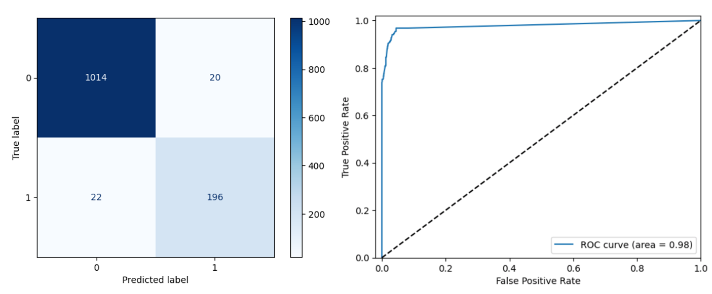
Figure 4: Confusion matrix and ROC curve for the Label Propagation algorithm with a KNN kernel with 7 neighbors, an oversampling method SMOTE and 5% of the dataset already labeled.

The various resampling methods presented in section II-C3 were applied. The results are shown in table III. The difference in results between undersampling and oversampling can be explained by the fact that undersampling will reduce the number of majority, this leads to loss of data and loss of information from this data. On the contrary, oversampling increases the number of values in the minority class, providing more data. In our case, SMOTE is the best oversampling method. SMOTE selects a minority class instance and identifies its k-nearest neighbors in the feature space. It then creates new synthetic examples along the line segments connecting the selected instance and its neighbors. By introducing these synthetic examples, SMOTE effectively increases the size of the minority class, making it comparable to the majority class and improving the performance of classifiers in handling imbalanced datasets.

TABLE IV: A comparison of the performance of different classifiers for the class ”with artifact”

Model	Precision	Recall	F1	AUROC
KNN	0.89	0.95	0.92	0.98
MLP	0.76	0.97	0.85	0.99
Transformer	0.85	0.86	0.85	0.97
ConvolutionNN Baseline Classifier	0.86	0.83	0.84	0.95

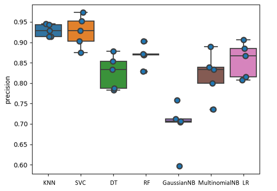
Figure 5: Precision evaluation for different traditional Machine Learning classifiers (in axis order: KNN, SVC, Decision Tree, Random Forest, Gaussian NB, Multinomial NB, Logistic Regression).

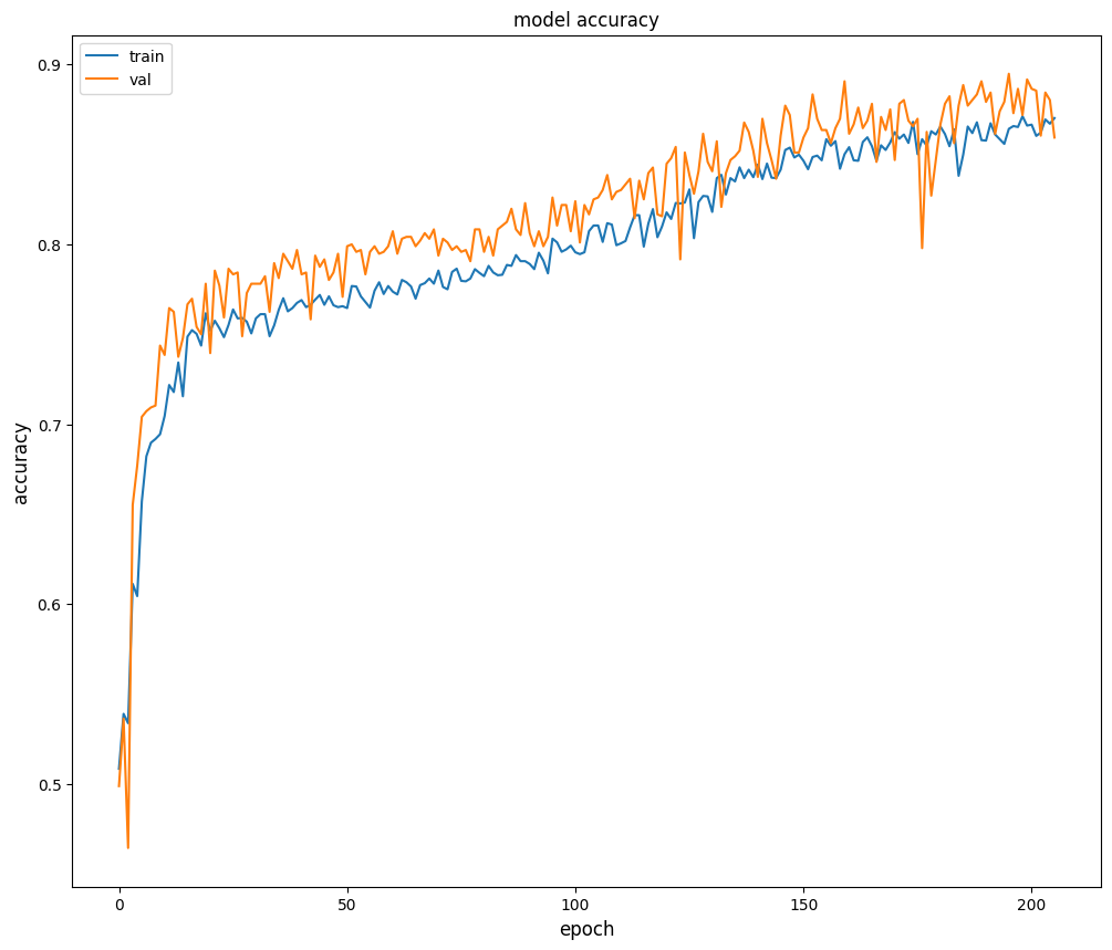
Figure 6: Accuracy curve during training and validation for the FCN model.

Given the correct sampling method and the appropriate proportion of the dataset to be selected, the results of the Label Propagation algorithm were evaluated. The confusion matrix is shown on the left and the ROC curve on the right, on the Fig. 4. The ROC curve is plotted for each decision threshold. In the case of the label propagation algorithm, this represents the probability assigned to each instance for each class. For a 5% dataset, the number of pulses for the validation part is 1252 pulses. 1034 belong to the ”without artifacts” category and 218 to the ”with artifacts” category. The number of true positives and true negatives is higher than the number of false positives or false negatives. This indicates that the algorithm is correctly able to understand the model and apply it to unlabeled signals. However, the number of pulses detected as clean but actually containing artifacts (false negatives) is higher than the reverse (false positives). This is because the Label Propagation algorithm uses neighborhood information to propagate labels through the data network. This means that labels for samples close in feature space tend to be similar. However, in the case of pulses containing artifacts, these artifacts may be similar to certain features of other clean pulses, leading to incorrect label propagation. As a result, pulses containing artifacts may be incorrectly labeled as clean by the Label Propagation algorithm, leading to a higher number of falsely classified pulses. Having misclassified pulses is always a problem that is important in the medical field. This can lead to false alarms, if the pulse is not a clean pulse, or to misdetections. False alarms force hospital staff to make emergency visits due to outliers. These situations are exhausting, and not necessary as an additional burden on caregivers. The area under the ROC curve (AUROC) is 0.97. The closer the AUROC is to 1, the better the model’s performance. A high AUROC indicates that our model is able to discriminate well between positive and negative classes.

After evaluating the Label Propagation algorithm, the performance of the different types of classifiers, presented in section II-D, were assessed. First, dealing with the imbalanced classes by oversampling using Adaptive Synthetic (ADASYN) algorithm. Cross-validation was employed to ensure accurate model prediction and assess the reliability of the machine learning algorithms. The results of the 5-fold cross-validation on different classifiers are presented in Fig. 5, which shows a precision comparison using a box plot. Each blue dot represents the performance of an individual fold in the cross-validation. The figure indicates that KNN and SVC (with a kernel of ’rbf’) are the top-performing classifiers, with median precision rates above 90%. However, KNN shows a slightly better and more consistent performance than SVC. This observation is highlighted by the broader range of variability for SVC, as indicated by the whiskers on the box plot, compared to KNN. To sum up, KNN and SVC are the top classifiers, but KNN is the more reliable and stable solution. KNN is also the best classifier compared to classifiers that use neural networks such as MLP and Transformers. Table IV shows the different performances of the neural networks classifiers: MLP classifier, Transformer, ConvolutionNN VS KNN classifier. MLP consists of 3 hidden layers with 500 neurons for each hidden layer. Its macro average accuracy (calculates the accuracy for each class individually and then computes the average accuracy across all classes) is 0.88, compared with 0.94 for KNN. In our case, using a complex model like MLP could lead to overfitting, as the model may have a high capacity relative to the amount of data available. In addition, training an MLP can be computationally expensive, especially with larger architectures and limited computational resources. Transformers, especially large ones like BERT (Bidirectional Encoder Representations from Transformers), have a high computational complexity and require significant computational resources for training and inference. Like the MLP classifier, Transformers works best on larger datasets because it needs a lot of data for the training part, otherwise the model has a greater capacity than the limited number of data and the risk is overfitting. Generally speaking, in the medical field, Transformers excel in natural language processing tasks [34]. They can learn complex relationships and patterns within the text, making them suitable for tasks involving medical text classification and understanding.

For the last classifier, experiments were conducted with a Fully Convolutional Network (FCN). FCN is a neural network architecture designed for semantic segmentation, producing dense pixel-wise predictions. It consists of convolutional layers without fully connected layers, enabling it to handle images of any size and preserve spatial information. Using FCN for time series classification involves adapting the fully convolutional architecture to process one-dimensional time series data. Instead of working with two-dimensional images, the FCN is applied to sequences of data points. The temporal convolutional layers capture temporal patterns and dependencies in the time series, and the decoding path with transposed convolutional layers helps to produce dense predictions for each data point in the sequence, enabling accurate time series classification [35]. One key benefit is that FCN eliminate the need for manual feature engineering, as they can directly learn relevant features from raw time series data. This streamlines the classification process and saves time and effort in designing handcrafted features. Additionally, FCN enable end-to-end learning, optimizing feature representations and classification jointly, which can lead to improved performance. The flexibility of FCN with input size allows them to handle time series data of varying lengths without requiring resizing or padding, making them suitable for irregularly sized data. Moreover, FCN produce dense predictions for each time step, capturing fine-grained temporal patterns and enhancing the informativeness of classification results. Experimentally, during FCN training, it is evident that the process takes longer than other approaches. However, its performance is not comparable to those methods, mainly due to its lower accuracy. Moreover, the Fig. 6 shows that both the validation and training accuracy display fluctuations, indicating a lack of stability in its performance.

V Conclusion

In conclusion, this study delved into utilizing semi-supervised label propagation (LP) methods for artifact classification within PPG signals, especially in scenarios characterized by imbalanced class distributions. To validate the effectiveness of this approach, we compared the results from the semi-supervised LP method against those obtained using traditional supervised learning algorithms, MLP, and Transformer-based models. Based on the experimental results, with oversampling method, the Label Propagation classifier performs better than neural network classifiers, MLP, FCN, and Transformers, achieving precision, recall, and F1 scores of 91%, 90%, and 90%, respectively. In particular, the performance of Label Propagation is comparable to that of KNN (k=3), which attains a higher recall score of 95% and an F1 score of 92%. However, the label propagation performs more consistently with a balanced precision-recall trade-off, whereas the KNN classifier struggles in that aspect. For improvements and future work, some directions can be given:

• Improving the preprocessing: In section II-C2, the problem of segmentation has already been mentioned. Some steps can be added to the preprocessing part. First, adaptive filtering techniques can be used to attenuate artifacts without affecting the signal. Signal quality can be improved through noise reduction methods, such as singular value decomposition (SVD). To enhance the efficiency of the statistical analysis algorithm, alternative segmentation approaches can be employed. Peak or minima detection can be improved by employing derivative-based algorithms. A CNN model can also be used to detect peaks, known for its pattern recognition capabilities.

• Machine learning approaches: Adapting different methods for tackling labeling limitation like self-supervised or unsupervised learning approaches.

• Data augmentation: Exploring data augmentation methods to increase data availability for improving the classifier’s generalization.

Overall, the use of label propagation techniques for labeling and classifying artifacts detection in PPG signals presents a promising direction for more accurate and reliable healthcare monitoring systems.

Clara Macabiau is a double degree student in Canada. After three years at the ENSEEIHT engineering school in Toulouse, specializing in EEEA (Electronics, Electrical Energy and Automation), she is completing her master’s degree with a thesis in electrical engineering at the Ecole de Technologie Supérieure in Montreal. Her master’s project focused on the detection of artifacts in photoplethysmography signals from children admitted to pediatric intensive care at CHU Sainte-Justine. Her fields of interest are signal processing, machine learning and electronics.

Thanh-Dung Le (Member, IEEE) received a B.Eng. degree in mechatronics engineering from Can Tho University, Vietnam, an M.Eng. degree in electrical engineering from Jeju National University, S. Korea, and a Ph.D. in biomedical engineering from Ecole de Technologie Supérieure (ETS), Canada. He is a postdoctoral fellow at the Biomedical Information Processing Laboratory, ETS. His research interests include applied machine learning approaches for biomedical informatics problems. Before that, he joined the Institut National de la Recherche Scientifique, Canada, where he researched classification theory and machine learning with healthcare applications. He received the merit doctoral scholarship from Le Fonds de Recherche du Quebec Nature et Technologies. He also received the NSERC-PERSWADE fellowship, Canada, and a graduate scholarship from the Korean National Research Foundation, S. Korea.

Kévin Albert is physiotherapist, graduated from EUSES School of Health and Sport (2018 - Girona, Spain). He developed clinical expertise in the field of function rehabilitation after neuro-traumatic injury (France) and in cardio-respiratory rehabilitation (Swiss). He is currently enrolled in the Master’s Biomedical Engineering program at the University of Montreal and has joined the Clinical Decision Support System (CDSS) laboratory under the supervision of Prof. P. Jouvet M.D. Ph.D. in the Pediatric Intensive Care Unit at Sainte-Justine Hospital (Montréal, Canada) since May 2023. His primary research interest is application new technologies of support care system tool with artificial intelligence, especially in ventilatory support. His research program is supported by the Sainte-Justine Hospital and the Quebec Respiratory Health research Network (QRHN).

Mana Shahriari is an artificial intelligence (AI) researcher passionate about employing AI to address practical and real-world challenges. Her research interests are signal processing (including time-series analysis), image processing and computer vision, machine learning and deep earning, and statistical analysis of data. She is currently a postdoctoral researcher at CHU Sainte Justine research centre, affiliated with University of Montreal. She holds a Ph.D. in electrical engineering, a Master’s in Artificial Intelligence, and a bachelor’s in electrical engineering.

Philippe Jouvet received the M.D. degree from Paris V University, Paris, France, in 1989, the M.D. specialty in pediatrics and the M.D. subspecialty in intensive care from Paris V University, in 1989 and 1990, respectively, and the Ph.D. degree in pathophysiology of human nutrition and metabolism from Paris VII University, Paris, in 2001. He joined the Pediatric Intensive Care Unit of Sainte Justine Hospital—University of Montreal, Montreal, QC, Canada, in 2004. He is currently the Deputy Director of the Research Center and the Scientific Director of the Health Technology Assessment Unit, Sainte Justine Hospital–University of Montreal. He has a salary award for research from the Quebec Public Research Agency (FRQS). He currently conducts a research program on computerized decision support systems for health providers. His research program is supported by several grants from the Sainte-Justine Hospital, Quebec Ministry of Health, the FRQS, the Canadian Institutes of Health Research (CIHR), and the Natural Sciences and Engineering Research Council (NSERC). He has published more than 160 articles in peer-reviewed journals. Dr. Jouvet gave more than 120 lectures in national and international congresses.

Rita Noumeir (Member, IEEE) received master’s and Ph.D. degrees in biomedical engineering from École Polytechnique of Montreal. She is currently a Full Professor with the Department of Electrical Engineering, École de Technologie Superieure (ETS), Montreal. Her main research interest is in applying artificial intelligence methods to create decision support systems. She has extensively worked in healthcare information technology and image processing. She has also provided consulting services in large-scale software architecture, healthcare interoperability, workflow analysis, and technology assessment for several international software and medical companies, including Canada Health Infoway.

References

- [1] J. M. Helm et al., “Machine learning and artificial intelligence: definitions, applications, and future directions,” Current reviews in musculoskeletal medicine, vol. 13, no. 1, pp. 69–76, 2020.
- [2] S. Dash et al., “Big data in healthcare: management, analysis and future prospects,” Journal of Big Data, vol. 6, no. 54, 2019.
- [3] G. Gutierrez, “Artificial intelligence in the intensive care unit,” Critical Care, vol. 24, no. 1, p. 101, 2020.
- [4] L. Ho et al., “The dependence of machine learning on electronic medical record quality,” in AMIA Symposium, 2018, pp. 883–891.
- [5] L. N. Sanchez-Pinto and R. G. Khemani, “Development of a prediction model of early acute kidney injury in critically ill children using electronic health record data,” Pediatric Critical Care, vol. 17, no. 6, pp. 508–15, 2016.
- [6] E. Choi et al., “Using recurrent neural network models for early detection of heart failure onset,” Journal of the American Medical Informatics Association : JAMIA, vol. 24, no. 2, pp. 361–370, 2017.
- [7] H. Li et al., “Patient clustering improves efficiency of federated machine learning to predict mortality and hospital stay time using distributed electronic medical records,” Journal of Biomedical Informatics, vol. 99, p. 103291, 2019.
- [8] S. Dara et al., “Machine learning in drug discovery: a review,” Artificial Intelligence Review, vol. 55, no. 3, pp. 1947–1999, 2022.
- [9] K. Ngiam and I. Khor, “Big data and machine learning algorithms for health-care delivery,” The Lancet. Oncology, vol. 20, no. 5, pp. 262–273, 2016.
- [10] A. E. Johnson et al., “Machine learning and decision support in critical care,” Proceedings of the IEEE, vol. 104, no. 2, pp. 444–466, 2016.
- [11] H. Habehh and S. Gohel, “Machine learning in healthcare,” Current Genomics, vol. 22, no. 4, pp. 291–300, 2016.
- [12] D. Pollreisz and N. TaheriNejad, “Detection and removal of motion artifacts in ppg signals,” Mobile Networks and Applications, vol. 27, pp. 728–738, 2022.
- [13] M. T. Petterson et al., “The effect of motion on pulse oximetry and its clinical significance,” Anesthesia & Analgesia, vol. 105, no. 6, pp. 78–84, 2007.
- [14] S.-H. Kim et al., “Accuracy and precision of continuous noninvasive arterial pressure monitoring compared with invasive arterial pressure: a systematic review and meta-analysis,” Anesthesiology, vol. 120, no. 5, pp. 1080–1097, 2014.
- [15] B. L. Hill et al., “Imputation of the continuous arterial line blood pressure waveform from non-invasive measurements using deep learning,” Scientific Reports, vol. 11, no. 1, p. 15755, 2021.
- [16] D. Bünger et al., “An empirical study of graph-based approaches for semi-supervised time series classification,” Frontiers in Applied Mathematics and Statistics, vol. 7, 2022.
- [17] Mazurowski et al., “Training neural network classifiers for medical decision making: The effects of imbalanced datasets on classification performance,” Neural networks, vol. 21, no. 2, pp. 427–436, 2008.
- [18] Z. Xu and K. Funaya, “Time series analysis with graph-based semi-supervised learning,” in 2015 IEEE International Conference on Data Science and Advanced Analytics (DSAA), 2015, pp. 1–6.
- [19] Y. Shin et al., “Coherence-based label propagation over time series for accelerated active learning,” in International Conference on Learning Representations, 2021.
- [20] D. E. Robbins et al., “Information architecture of a clinical decision support system,” in 2011 Proceedings of IEEE Southeastcon. IEEE, 2011, pp. 374–378.
- [21] A. J. Aljaaf et al., “Applied machine learning classifiers for medical applications: clarifying the behavioural patterns using a variety of datasets,” in 2015 International Conference on Systems, Signals and Image Processing (IWSSIP). IEEE, 2015, pp. 228–232.
- [22] D. Brossier et al., “Creating a high-frequency electronic database in the picu: The perpetual patient,” Pediatric critical care medicine, vol. 19, no. 4, pp. 189–198, 2018.
- [23] N. Roumeliotis et al., “Reorganizing care with the implementation of electronic medical records: A time-motion study in the picu,” Pediatric critical care medicine, vol. 19, no. 4, pp. 172–179, 2018.
- [24] A. Mathieu et al., “Validation process of a high-resolution database in a paediatric intensive care unit-describing the perpetual patient’s validation,” Journal of Evaluation in Clinical Practice, vol. 27, no. 2, pp. 316–324, 2021.
- [25] P. Lim et al., “Adaptive template matching of photoplethysmogram pulses to detect motion artefact,” Physiological measurement, vol. 39, no. 10, p. 105005, 2018.
- [26] Q. Li and G. Clifford, “Dynamic time warping and machine learning for signal quality assessment of pulsatile signals,” Physiological measurement, vol. 33, no. 9, pp. 1491–1501, 2012.
- [27] S. Hanyu and C. Xiaohui, “Motion artifact detection and reduction in ppg signals based on statistics analysis,” in 2017 29th Chinese Control And Decision Conference (CCDC), 2017, pp. 3114–3119.
- [28] R. Krishnan et al., “Analysis and detection of motion artifact in photoplethysmographic data using higher order statistics,” 03 2008, pp. 613–616.
- [29] K. Fujiwara et al., “Over- and under-sampling approach for extremely imbalanced and small minority data problem in health record analysis,” Frontiers in Public Health, vol. 8, 2020.
- [30] X. Zhu and Z. Ghahramani, “Learning from labeled and unlabeled data with label propagation,” School of Computer Science, 2002.
- [31] Z. Song et al., “Graph-based semi-supervised learning: A comprehensive review,” IEEE Transactions on Neural Networks and Learning Systems, pp. 1–21, 2022.
- [32] Z. Bodo and L. Csató, “A note on label propagation for semi-supervised learning,” Acta Universitatis Sapientiae, Informatica, vol. 7, 2015.
- [33] R. Miotto et al., “Deep learning for healthcare: review, opportunities and challenges,” Briefings in bioinformatics, vol. 19, no. 6, pp. 1236–1246, 2018.
- [34] V. Yogarajan et al., “Transformers for multi-label classification of medical text: an empirical comparison,” in International Conference on Artificial Intelligence in Medicine, 2021, pp. 114–123.
- [35] Z. Wang et al., “Time series classification from scratch with deep neural networks: A strong baseline,” in 2017 International joint conference on neural networks (IJCNN). IEEE, 2017, pp. 1578–1585.