Eliciting Risk Aversion with Inverse Reinforcement Learning via Interactive Questioning

Abstract:

This paper proposes a novel framework for identifying an agent’s risk aversion using interactive questioning. Our study is conducted in two scenarios: a one-period case and an infinite horizon case. In the one-period case, we assume that the agent’s risk aversion is characterized by a cost function of the state and a distortion risk measure. In the infinite horizon case, we model risk aversion with an additional component, a discount factor. Assuming the access to a finite set of candidates containing the agent’s true risk aversion, we show that asking the agent to demonstrate her optimal policies in various environment, which may depend on their previous answers, is an effective means of identifying the agent’s risk aversion. Specifically, we prove that the agent’s risk aversion can be identified as the number of questions tends to infinity, and the questions are randomly designed. We also develop an algorithm for designing optimal questions and provide empirical evidence that our method learns risk aversion significantly faster than randomly designed questions in simulations. Our framework has important applications in robo-advising and provides a new approach for identifying an agent’s risk preferences.

Keywords:

imitation learning, design of experiments, distortion risk measures, robo-advising

1 Introduction

The prevailing belief that behavioral demonstrations reflect human values has led to the development of inverse reinforcement learning (IRL), a field dedicated to understanding an agent’s objectives through their behavior. Specifically, IRL aims to estimate an agent’s reward (or cost) function by observing their assumed optimal policy within a known environment (cf. [26, 1, 31, 29, 42]). We also refer to [7, 3] for surveys on recent progress of IRL.

Most studies in IRL operate under the assumption that the agent is risk-neutral toward uncertainty. However, this assumption, often made for simplicity, may not accurately reflect real-world values. A comprehensive model of human values should likely include components that describe risk aversion toward uncertainty in addition to cost functions. Therefore, it is crucial to develop methods capable of providing corresponding estimations.

The study of human risk aversion toward uncertainty has been extensively conducted in the fields of economics, finance and psychology (cf. [12, 25, 34, 13, 40] and the references therein). While these investigations naturally demand the modeling capacity provided by modern computational power, the related exposition within an IRL context has been limited. To the best of our knowledge, a related study was first initiated in [24]. In this work, the authors use coherent risk measures (CRMs), introduced in [8, 18], to model the risk aversion. The proposed IRL method is further investigated in [36]. The numerical efficiency of this method was improved in [14] through the adoption of an active learning framework, which allows for querying the agent for additional demonstrations. We would also like to draw attention to [30], where the risk aversion is modeled from the standpoint of prospect theory.

As pointed out in [26], one major challenge in IRL is identifiability. This challenge becomes even more pronounced when estimating CRMs in addition to the cost function. Under certain assumptions, including the known and strictly convex cost, identifiability was established in a one-period case in [36]. The question of CRM identifiability in an IRL context largely remains unresolved.

In a risk neutral setting, there has been numerous studies addressing the identifiability of rewards. For instance, [19] proposes using an adversarial reward learning formulation. [20] and the references therein showcase that learning from exploring agents alleviates the identifiability issue given a limited amount of agent’s demonstrations. [22] embeds the domain of a Markov decision process model into a graph and reasons about how properties of the graph relate to identifiability. [37] formally characterizes the partial identifiability of the reward function and analyze the impact of partial identifiability.

While the extant literature show promising potential in handling the identifiability issue, in this paper, we are particularly interested in the framework where we as learners are allowed to design the environment in which the agent operates. [6, 5] establish the identifiability for reward function that depends only on the state, in a setting where the agent faces multiple tasks designed by the learner. A related setting appears in [11] to study identifiability with more general rewards. We refer to [9, 10] for simulations showcasing the effectiveness of the design in various scenarios. Beyond the risk neutral setting, [17] formulates a constrained optimization problem based on a series of assessments that infer the client’s risk aversion, as modeled by CRM, with solution methods for such constrained optimization further studied in [23]. Rather than directly addressing the identifiability, these two studies provide an alternative perspective on the issue.

In this paper, we aim to further explore the potential of environment design in IRL. Our study is conducted within a discrete world and is divided into two scenarios: a one-period case and an infinite horizon case. In the one-period case, we model the agent’s risk aversion with a cost function of the state and a spectral risk measure (SRM), which was popularized in [2] as a special, but very useful, class of CRMs. For the infinite horizon case, the agent assesses the temporal effect with a discount factor, which is also a component of the agent’s risk aversion unknown to us, and that the environment is stationary. Furthermore, we assume that the sequential decision making of the agent in the infinite horizon adheres to the risk averse dynamic programming principle proposed in [33] with a similar SRM used in one-period case. In the one-period case, we can design the probability of a state’s occurrence; in the infinite horizon case, we can design the transition matrix. After designing the environment, the agent, in turn, provides an optimal action or policy based on her own risk aversion, and this interaction repeats over multiple rounds.

To facilitate identifiability, we assume a finite set of candidate risk aversions that includes the agent’s true risk aversion. In this setting, identifiability can be resolved by establishing the existence of an environment leading to distinct optimal actions when two distinct risk aversions are considered. We present the desired existence results for the one-period case and the infinite horizon case in Theorem 3.2 and Theorem 3.3, respectively.

For implementation, we propose the use of Gibbs measures based on the regrets of the agent’s action or policy under hypothetical risk aversions. We argue that by properly choosing the learning rate, this Gibbs measure approach resembles the procedure that eliminates candidate risk aversions individually via the aforementioned theorems, while potentially providing robustness against errors arising from the agent’s suboptimal decisions. We justify the use of regret-based Gibbs measure by showing in Proposition 4.2 and Proposition 4.4 that the Gibbs measures asymptotically concentrate on the true risk aversion when the environments are randomly selected. We further propose methods for designing the environment for faster convergence. These methods select the environment by optimizing certain heuristically induced criteria. We demonstrate their effectiveness in simulations by comparing with scenarios where the environments are randomly selected and show that, empirically, they converge much faster.

Our framework has important applications in robo-advising, where an algorithm-driven robot entity recommends a strategy according to the client’s preferences. For instance, one may think of obtaining a personalized long-term investment portfolio allocation strategy with minimal human intervention and periodical interactions with the robot. Robo-advisors usually elicit clients’ risk-reward preferences with questionnaires to gather information about the investor’s profile of the client. This paper illustrates how such robo-advisors may learn and identify the client’s preferences. A particularly relevant configuration is the canonical setup (see Remark 2.2), where the cost of a state is the state itself. In this canonical setup, the design of the environment is virtually the same as querying the agent for the more acceptable random losses, as tailored by the learner.

The remainder of the paper is structured as follows. We first introduce some notations and the detailed setup in Section 2. We then proceed to investigate identifiability in Section 3 by establishing the existence of distinguishing environments. Section 4 is dedicated to the discussion of environment design. We examine the proposed design methods in Section 5. Finally, we provide some discussions on potential further works in Section 6 and conclude the paper in Section 7.

2 Problem setup

Main Goal.

In this paper, our primary objective is to investigate the IRL problem for an agent’s risk aversion within an iterative experimental setting. This setting enables us to exercise complete control over the environment in which the agent operates. By observing the agent’s policy, which is presumed to be optimal given their risk aversion, we aim to deduce the agent’s risk aversion. Next, we give some notations for risk assessment and analyze the problem in two scenarios: the one-period case and the infinite horizon case.

Notations.

$\delta_{z}$ is the Dirac measure at $z$. For a finite set $\mathbb{S}$, we use $|\mathbb{S}|$ to denote the cardinality. For a real-valued random variable $Z$ , we let $F_{Z}$ be the CDF of $Z$, and define $F^{-1}_{Z}(u):=\inf\{r\in\mathbb{R}:F_{Z}(r)\geq u\}$.

Distortion Risk Measures.

Let $\mathcal{P}([0,1])$ be the set of Borel probability measures on $[0,1]$ and $\mathcal{P}_{0}([0,1]):=\{\mu\in\mathcal{P}([0,1]):\mu(1)=0\}$. Let $\mu\in\mathcal{P}_{0}([0,1])$. For a real-valued integrable random variable $Z$, we define the following

$$\rho_{\mu}(Z):=\int_{0}^{1}\operatorname{\mathrm{AV}@\mathrm{R}}_{1-\alpha}(Z)\;\mu(\operatorname{d\!}\alpha),$$ (2.1)

where, for $\eta\in(0,1]$,

$$\operatorname{\mathrm{AV}@\mathrm{R}}_{\eta}(Z):=\inf_{r\in\mathbb{R}}\left\{r+\frac{1}{\eta}\mathbb{E}((Z-r)_{+})\right\},$$ (2.2)

i.e., $\operatorname{\mathrm{AV}@\mathrm{R}}$ is the average value at risk also called conditional value-at-risk (cf. [32]). In particular, $\rho_{\delta_{0}}$ is the expectation, i.e.,

$$\rho_{\delta_{0}}(Z)=\operatorname{\mathrm{AV}@\mathrm{R}}_{1}(Z)=\mathbb{E}(Z).$$

This class of risk measures is convenient to characterize trade-offs between different risk-aware objectives, for instance with a convex combination $\mu=\gamma\,\delta_{0}+(1-\gamma)\,\delta_{\kappa}$ (with $\gamma\in(0,1)$, $\kappa\in(0,1]$) the agent emphasizes risk while still valuing gains. Let

$$\sigma_{\mu}(r):=\int_{[0,r]}\frac{1}{1-\alpha}\,\mu(\operatorname{d\!}\alpha),\quad r\in[0,1).$$ (2.3)

The result below regards the properties of $\rho_{\mu}$, the proof of which can be found in, for example, [2], [35, Section 6.3.4].

Lemma 2.1.

Let $\mu\in\mathcal{P}_{0}([0,1])$ and $\sigma_{\mu}$ be defined in (2.3). Then, $\sigma_{\mu}$ is nonnegative, nondecreasing, right continuous, and $\int_{0}^{1}\sigma_{\mu}(r)\operatorname{d\!}r=1$. Moreover, $\sigma_{\mu}$ characterizes $\mu$ and $\rho_{\mu}$ in the following way

$$\mu([0,r]) =(1-r)\sigma_{\mu}(r)+\int_{0}^{r}\sigma_{\mu}(\alpha)\operatorname{d\!}\alpha,\qquad\alpha\in[0,1)$$

$$\rho_{\mu}(Z) =\int_{0}^{1}\sigma_{\mu}(\alpha)F^{-1}_{Z}(\alpha)\operatorname{d\!}\alpha.$$ (2.4)

For future reference, we provide a formula for computing $\rho_{\mu}(Z)$, when $Z$ is a real-valued random variable with finite support. Suppose $d\in\mathbb{N}$ and $0=z_{0}<\dots<z_{d}$. Consider a discrete real-valued random variable $Z$ taking values $z_{k}$ with probability $p_{k}$ where $\sum_{k=0}^{d}p_{k}=1$. By Lemma2.1, we have

$$\rho_{\mu}(Z)=\sum_{k=1}^{d}z_{k}\int_{P_{k-1}}^{P_{k}}\sigma_{\mu}(\alpha)\operatorname{d\!}\alpha,$$ (2.5)

where $P_{k}:=\sum_{i=0}^{k}p_{i}$ for $k=0,1,\dots,d$.

One period case.

Let $\mathbb{X}$ and $\mathbb{A}$ be finite state and action spaces. We model the agent’s risk aversion by $(C,\mu)$, where $C:\mathbb{X}\to\mathbb{A}$ is a cost function and $\mu\in\mathcal{P}_{0}([0,1])$ characterizes her risk measure. Let $C_{0}:\mathbb{X}\to\mathbb{R}$ and $\mu_{0}\in\mathcal{P}_{0}([0,1])$ be the ground truth. To deduce the agent’s risk aversion, at every round $n$, we design an environment $G_{n}:=(P_{n}^{a})_{a\in\mathbb{A}}\in\mathcal{P}(\mathbb{X})^{\mathbb{A}}$, where $P^{a}\in\mathcal{P}(\mathbb{X})$ is a simplex on $\mathbb{X}$. Provided $G_{n}$, the agent in turn demonstrates an optimal action subject to $G_{n}$, that is the agent provides the learner with

$$a_{n}^{*}\in\operatorname*{arg\,min}_{a\in\mathbb{A}}\rho_{\mu_{0}}\big{(}C_{0}(X^{a}_{G_{n}})\big{)},\quad\text{where }X^{a}_{G_{n}}\sim P^{a}_{n}.$$ (2.6)

Upon observing $a_{n}^{*}$, together with the observation from previous rounds, we design the next environment $G_{n+1}$. This process repeats itself for a given number of rounds, and our goal is to determine $(C_{0},\mu_{0})$. For simplicity, we assume the true risk aversion belongs to a finite set

$$\Upsilon:=\{(C_{0},\mu_{0}),(C_{1},\mu_{1}),\dots,(C_{L},\mu_{L})\}.$$

Remark 2.2.

Sometimes, it is fitting to consider a scenario where the cost of a state is represented by the state itself. We call this the canonical setup. For example, in canonical setup, $\mathbb{X}=\{0,0.5,1\}$ are the losses and the cost function is defined $C(x)=x$. This approach is particularly useful in questionnaires where the agent is asked to choose between two random losses, selecting the one they perceive to be less detrimental. $\blacksquare$

Remark 2.3.

Suppose the cost is known to take values from $[0,b]$. It would be ideal to formulate the problem without restricting ourselves to a finite set of candidates, $\Upsilon$, but to elicit risk aversion from $[0,b]^{|\mathbb{X}|}\times\mathcal{P}([0,1])$. The usage of $\Upsilon$ in this context is mainly for simplicity, as we are in the early stages of study.

On the other hand, we believe that a properly constructed $\Upsilon$, even without correctly containing the true risk aversion $(C_{0},\mu_{0})$, can achieve a small misspecification error. We may define the misspecification error as

$$\min_{(C,\mu)\in\Upsilon}\left|\rho_{\mu_{0}}(C_{0}(X_{0}))-\rho_{\mu}(C(X_{0}))\right|,$$

where $X_{0}$ is an $\mathbb{X}$-valued random variable on which the learner will evaluate using the agent’s risk aversion. Alternatively, in the canonical setup (see Remark 2.2), we may define the misspecification error as

$$\min_{(C,\mu)\in\Upsilon}\left|\rho_{\mu_{0}}(Z_{0})-\rho_{\mu}(Z_{0})\right|,$$

where $Z_{0}$ is a $[0,b]$-valued random variable. It is clear that $[0,b]^{|\mathbb{X}|}$ can be harmlessly discretized. Regarding $\mathcal{P}([0,1])$, we may invoke the compactness under weak topology (cf. [4, Section 15.3, 15.11]) and the fact that, for bounded real-valued random variable $Z$, $\eta\mapsto\operatorname{\mathrm{AV}@\mathrm{R}}_{\eta}(Z)$ is continuous in $\zeta\in(0,1]$ and can be continuously extended to $\zeta=0$ (cf. [35, Section 6.2.4, Remark 22]). A more in-depth analysis on missepcification error will be pursued in further works.

Nevertheless, in practical settings, the true risk aversion of the agent may be different than the risk aversion candidates the learner postulates. We investigate the behavior of algorithms with different environment-design approaches in the event of model misspecification in Section 5. $\blacksquare$

Infinite horizon case.

When managing a sequence of losses, the discount factor $r\in(0,1)$ is an important component. More precisely, we characterize the agent’s risk aversion with the triplet $(C,\mu,r)$, where $C:\mathbb{X}\to\mathbb{R}$ is the stationary cost, $\mu$ is a probability on $(0,1)$, and $r\in(0,1)$ represents the discount factor. We will detail our model of the agent’s decision-making process shortly in Definition 2.5 below.

Here, we develop the learning environment in the stationary infinite horizon context. This involves considering an infinite horizon stationary Markov Decision Process (MDP) with a finite state space $\mathbb{X}$ and action space $\mathbb{A}$. We assume the MDP’s controlled transition matrix is constant in time and the admissible domain of actions is always $\mathbb{A}$.

Remark 2.4.

In this remark, we provide some rationale behind the use of a stationary infinite horizon setting. In real world settings, decision making typically has a finite horizon. It is, however, often impractical to reverse-engineer every potential outcome for long-term decision making. It is plausible to assume that long-term decisions are formed by stringing together a series of short-term (myopic) choices, possibly facilitated by disregarding uncertainties in the distant future. While this may be a simplification, we model such disregard with a discount factor $r\in(0,1)$. The presence of this discount factor implies that decisions made in a stationary environment with a relatively large time frame may resemble those made within an infinite horizon. Take, for instance, the context of trading where an agent adjusts the portfolio on a daily basis. In such scenarios, using a stationary infinite horizon approach for approximation may be appropriate, even with its inherent simplifications. $\blacksquare$

Below we provide the detailed description on how the agent makes decisions under the risk aversion $(C,\mu,r)$. We assume the agent uses a stationary ‘deterministic’ action $\pi:\mathbb{X}\to\mathbb{A}$. We use $\Pi$ to denote the space of allowed actions, which can be equivalently viewed as $\mathbb{A}^{\mathbb{X}}$. Let ${\widetilde{G}}:=(T^{a})_{a\in\mathbb{A}}\in\mathcal{T}(\mathbb{X})^{\mathbb{A}}$ be a controlled transition dynamic, where $\mathcal{T}(\mathbb{X})$ is the set of transition matrices on $\mathbb{X}$. The learner chooses the transition dynamics ${\widetilde{G}}$ and any initial state $i_{0}\in\mathbb{X}$ freely. Subsequently, the agent evaluates a policy $\pi\in\Pi$ with $\varrho_{C,\mu,r}^{i_{0},\infty}\left(\pi;{\widetilde{G}}\right)$ defined below.

Definition 2.5.

We first introduce $R^{\pi,{\widetilde{G}}}_{C,\mu,r}:\ell^{\infty}(\mathbb{X})\to\ell^{\infty}(\mathbb{X})$ by how it acts on functions $u\in\ell^{\infty}(\mathbb{X})$ as follows

$$R^{\pi,{\widetilde{G}}}_{C,\mu,r}u(x):=C(x)+r\,\rho_{\mu}\left(u\left(X^{x,\pi(x)}_{{\widetilde{G}}}\right)\right),\quad X^{x,a}_{{\widetilde{G}}}\sim T^{a}_{x},$$

where $T^{a}_{x}$ is the $x$-row of $T^{a}$. Let $O\equiv 0$. For $\tau\in\mathbb{N}$, we then let

$$\varrho^{x,\tau}_{C,\mu,r}\left(\pi;{\widetilde{G}}\right):=\left(R^{\pi,{\widetilde{G}}}_{C,\mu,r}\right)^{\tau}O,\quad x\in\mathbb{X}$$

Finally, we define $\varrho_{C,\mu,r}^{x,\infty}\left(\pi;{\widetilde{G}}\right):=\displaystyle\lim_{\tau\to\infty}\varrho^{x,\tau}_{C,\mu,r}(\pi)$ for $x\in\mathbb{X}$.

It follows from the monotonicity and translation invariance of coherent risk measure (cf. [35, Section 6.3]) that the limit defining $\varrho_{C,\mu,r}^{x,\infty}(\pi)$ is valid and $\varrho_{C,\mu,r}^{x,\infty}(\pi)\leq(1-r)^{-1}\|C\|_{\infty}$. This type of performance criteria was first proposed by [33] and is now widely used in many disciplines, such as finance and autonomous robotics (cf. [16, 41] and the reference therein). It is known [33] that $\varrho_{C,\mu,r}^{\cdot,\infty}(\pi;{\widetilde{G}})$ is the unique solution of the fixed-point equation below with unknown $V\in\ell^{\infty}(\mathbb{X})$,

$$V(x)=R^{\pi,{\widetilde{G}}}_{C,\mu,r}V(x)=C(x)+r\left\{\rho_{\mu}\left(V\left(X^{x,a}_{\widetilde{G}}\right)\right)\right\},\quad x\in\mathbb{X},$$ (2.7)

and $\min_{\pi}\varrho_{C,\mu,r}^{\cdot,\infty}(\pi;{\widetilde{G}})$ is the unique solution of the fixed-point equation below with unknown $V^{*}\in\ell^{\infty}(\mathbb{X})$,

$$V^{*}(x)=\min_{\pi\in\Pi}R^{\pi,{\widetilde{G}}}_{C,\mu,r}V^{*}(x)=C(x)+r\min_{a\in\mathbb{A}}\left\{\rho_{\mu}\left(V^{*}\left(X^{x,a}_{\widetilde{G}}\right)\right)\right\},\quad x\in\mathbb{X},$$ (2.8)

Moreover, if $\pi^{*}:\mathbb{X}\to\mathbb{A}$ satisfies

$$\pi^{*}(x)\in\operatorname*{arg\,min}_{a\in\mathbb{A}}\left\{R^{\pi,{\widetilde{G}}}_{C,\mu,r}V^{*}(x)\right\}=\operatorname*{arg\,min}_{a\in\mathbb{A}}\rho_{\mu}\left(V^{*}\left(X^{x,a}_{\widetilde{G}}\right)\right),\quad x\in\mathbb{X},$$ (2.9)

then $\pi^{*}$ is the optimal action. Furthermore, it can be shown that under the setup above, particularly when $\rho_{\mu}$ is a spectral risk measure, the optimal stationary Markovian deterministic action is optimal even when compared to all the history-dependent randomized policies; we refer to [15, Section 6] for detailed discussion.

We consider a similar iterative scheme as in the one period case. Let $(C_{0},\mu_{0},r_{0})$ represents the risk aversion of the agent. At every round $n$, we design a controlled transition matrix ${\widetilde{G}}_{n}\in\mathcal{T}(\mathbb{X})^{\mathbb{A}}$ and the agent takes the optimal policy $\pi^{*}_{n}$, i.e.,

$$\pi_{n}^{*}(x)\in\operatorname*{arg\,min}_{a\in\mathbb{A}}\rho_{\mu_{0}}\left(V^{*}_{\widetilde{G}_{n},0}\left(X^{x,a}_{\widetilde{G}_{n}}\right)\right),\quad x\in\mathbb{X},$$ (2.10)

where

$$V^{*}_{\widetilde{G},\ell}(x):=\min_{\pi\in\Pi}\varrho_{C_{\ell},\mu_{\ell},r_{\ell}}^{x,\infty}\left(\pi;{\widetilde{G}}\right),\quad x\in\mathbb{X}.$$ (2.11)

For simplicity, we assume that we have full access to the agent’s optimal policy through demonstration. We also assume the knowledge that the agent’s risk aversion is contained by a finite set of candidates $\Xi:=\{(C_{0},\mu_{0},r_{0}),(C_{1},\mu_{1},r_{1}),\dots,(C_{L},\mu_{L},r_{L})\}$.

3 Identifiability

The interactive environment provides us with the means to identify the risk aversion of the agent, in the setting where we assume a finite set of candidates. Idenfiability of the agent’s risk aversion can be achieved by establishing the existence of a distinguishing environment for any two distinct risk aversions. Specifically, a distinguishing environment leads to different optimal actions or policies corresponding to the respective risk aversions. To rigorously establish the said existence, we make the following technical assumptions.

Assumption 3.1.

The following is true for $\ell\in\{0,\dots,L\}$:

1. $|\mathbb{X}|\geq 3$ and $|\mathbb{A}|\geq 2$;

2. $C_{\ell}$ is one-to-one, $\displaystyle\min_{x\in\mathbb{X}}C_{\ell}(x)=0$ and $\displaystyle\max_{x\in\mathbb{X}}C_{\ell}(x)=1$;

3. $\sigma_{\mu_{\ell}}$ is bounded.

It is important that $C_{0}$ takes at least $3$ different values. To see this in the one-period case, notice that if $C_{0}$ takes only $2$ values, say $C_{0}:\mathbb{X}\to\{c_{1},c_{2}\}$ for some $c_{1}>c_{2}$, then $a^{*}$ satisfies (2.6) if and only if

$$\mathbb{P}\big{(}C_{0}(X^{a^{*}}_{G})=c_{1}\big{)}\leq\mathbb{P}\big{(}C_{0}(X^{a}_{G})=c_{1}\big{)},\quad a\in\mathbb{A},$$

regardless of the specific values of $c_{1}$, $c_{2}$ and $\mu_{0}$. As a result, different $(C_{0},\mu_{0})$’s can result in the same optimal action for all $G\in\mathcal{P}(\mathbb{X})^{\mathbb{A}}$, which hinders the identifiability. Regarding condition (ii), the one-to-one property of $C_{\ell}$ is imposed primarily for the sake of convenience. While it is possible to remove this condition, doing so would require a tedious case-by-case discussion that provides little additional insight. The rest of condition (ii) is a harmless rescaling assumption, due to the translation invariance and positive homogeneity of coherent risk measure (cf. [35, Section 6.3]). Finally, condition (iii) imposes the boundedness for $\sigma_{\mu_{\ell}}$. This condition plays a crucial technical role in establishing the subsequent results on the existence of a distinguishing environment (see the proof of Lemma A.2). We recognize, however, the significance of exploring identifiability without this condition. The related results will be pursued in the future work.

Below we present two results. The first result, Theorem 3.2, regards the existence of a distinguishing environment in the one-period case. For illustration, we provide an example of such a environment in Figure 1. In this example, we assume the two risk aversions share the same $C$ but have different Dirac $\mu$’s. The construction of a distinguishing environment for proving Theorem 3.2 is less straightforward, and we refer to Appendix A.1 for the details.

Theorem 3.2.

Suppose the one-period setting depicted in Section 2 and Assumption 3.1 both hold. For any different $(C,\mu),(C^{\prime},\mu^{\prime})\in\Upsilon$, there exists $G\in\mathcal{P}(\mathbb{X})^{\mathbb{A}}$ such that

$$\operatorname*{arg\,min}_{a\in\mathbb{A}}\rho_{\mu}\left(C(X^{a}_{G})\right)\cap\operatorname*{arg\,min}_{a\in\mathbb{A}}\rho_{\mu^{\prime}}\left(C^{\prime}(X^{a}_{G})\right)=\emptyset.$$

Figure 1: Illustration of a separating environment.

Suppose $\mathbb{X}=\{x_{0},x_{1},x_{2}\}$, $\mathbb{A}=\{a_{1},a_{2}\}$ and $C(x_{1})=c\in(0,1)$ is known. We consider $0<\kappa<\kappa^{\prime}<1$ and set $\mu=\delta_{1-\kappa}$, $\mu^{\prime}=\delta_{1-\kappa^{\prime}}$, i.e., $\rho_{\mu}=\operatorname{\mathrm{AV}@\mathrm{R}}_{\kappa}$ and $\rho_{\mu^{\prime}}=\operatorname{\mathrm{AV}@\mathrm{R}}_{\kappa^{\prime}}$. Let $P^{a_{1}}=(1-p,p,0)$ and $P^{a_{2}}=(1-q,0,q)$. Values of $p$ and $q$ affect the optimal actions under $\rho_{\mu}$ and $\rho_{\mu^{\prime}}$. The blue region is where $(p,q)$ make the the optimal actions under $\rho_{\mu}$ and $\rho_{\mu^{\prime}}$ distinct.

The second result, Theorem 3.3, is the infinite horizon counterpart to Theorem 3.2. In its proof, we first examine a scenario where $(C,\mu)\neq(C^{\prime},\mu^{\prime})$ and $r,r^{\prime}$ may or may not differ. By leveraging Theorem 3.2 and exploiting the freedom to choose the controlled transition matrix $\widetilde{G}$, we establish the existence of a distinguishing environment. Subsequently, we investigate the situation where $(C,\mu)=(C^{\prime},\mu^{\prime})$ but $r\neq r^{\prime}$. A distinguishing environment can be constructed accordingly. The details of the proof is deferred to Appendix A.2.

Theorem 3.3.

Suppose the infinite horizon setting depicted in Section 2 and Assumption 3.1 both hold. For any different $(C,\mu,r),(C^{\prime},\mu^{\prime},r^{\prime})\in\Xi$, there exists ${\widetilde{G}}\in\mathcal{T}(\mathbb{X})^{\mathbb{A}}$ such that

$$\operatorname*{arg\,min}_{\pi:\mathbb{X}\to\mathbb{A}}\varrho^{x,\infty}_{C,\mu,r}\left(\pi;{\widetilde{G}}\right)\cap\operatorname*{arg\,min}_{\pi:\mathbb{X}\to\mathbb{A}}\varrho^{x,\infty}_{C^{\prime},\mu^{\prime},r^{\prime}}\left(\pi;{\widetilde{G}}\right)=\emptyset\quad\text{for some}\quad x\in\mathbb{X}.$$

4 Design of environments

In this section, we propose a method that designs the environment for the next round based on outcomes of previous interactions. This method hinges on the concepts of regret and the associated Gibbs measure, which we introduce in Section 4.1. In particular, the Gibbs measure converts the environments and actions (policies) of the agent from previous rounds into a probability on $\{0,1,\dots,L\}$, reflecting our confidence on the candidate risk aversions. We discuss the design of environments based on these concepts in Section 4.2.

As elaborated below, utilizing regrets and the related Gibbs measure could be advantageous. On one hand, it integrates the intuitive learning procedure that eliminates candidate risk aversions individually (occasionally achieving collateral elimination), aligning closely with Theorem 3.2 and Theorem 3.3. On the other hand, it facilitates the development of a scheme that enables the bulk elimination of candidate risk aversions. Finally, although not explicitly addressed in this paper, we believe that an approach like the one we propose here could potentially provide some degree of robustness against errors arising from the agent selecting a suboptimal action.

4.1 Regrets and the associated Gibbs measure

We structure our discussion into two parts: the one-period case and the infinite horizon case. We note that, despite the differences in these two cases, the concepts of regret and the associated Gibbs measure are founded on similar principles.

One period case.

We start by introducing a notion of regret.

Definition 4.1.

We define the regret of action $a\in\mathbb{A}$ under environment $G\in\mathcal{P}(\mathbb{X})^{\mathbb{A}}$ and risk aversion $\ell\in\{0,1,\dots,L\}$ as

$$\Phi(a;G,\ell):=\rho_{\mu_{\ell}}(C_{\ell}(X^{a}_{G}))-\min_{k\in\mathbb{A}}\rho_{\mu_{\ell}}\left(C_{\ell}\left(X^{k}_{G}\right)\right).$$ (4.1)

That is, the regret is the excess risk the agent takes on if they choose the action $a$ compared to the optimal one. Clearly, $\Phi\geq 0$, and $a\in\operatorname*{arg\,min}_{\theta}V(\theta,G,\ell)$ if and only if $\Phi(a,G,\ell)=0$. Since $G\mapsto\rho_{\mu_{\ell}}(C_{\ell}(X^{a}_{G}))$ is continuous due to (2.5), and $\mathbb{A}$ is finite, we have $G\mapsto\Phi(a;G,\ell)$ is continuous.

Let $(G_{n})_{n=1}^{N}$ be a finite set of environments, $(a^{*}_{n})_{n=1}^{N}$ be the optimal action generated according to (2.6). We introduce below a Gibbs measure as the probability on the candidate risk aversions $\{0,1,\dots,L\}$:

$$\mathbb{Q}_{N}(\{\ell\})\propto\exp\left(-k\sum_{n=1}^{N}\Phi(a^{*}_{n};G_{n},\ell)\right),$$ (4.2)

where $k>0$ is a learning parameter.

Built upon Theorem 3.2, the next result regards the consistency of $(\mathbb{Q}_{N})_{N\in\mathbb{N}}$ when the $G_{n}$’s are IID samples from a uniform distribution on $\mathcal{P}(\mathbb{X})^{\mathbb{A}}$. More precisely, we let $d=|\mathbb{X}|-1\geq 2$ and consider the uniform distribution on $\mathcal{P}(\mathbb{X})$, denoted by $m$. In particular, for any $B\in\mathcal{B}(\mathbb{R}^{d+1})$,

$$m(B)=\int_{\mathbb{R}^{d}}\mathbbm{1}_{B}\left(1-\sum_{i=1}^{d}p_{i},p_{1},\dots,p_{d}\right)f(p_{1},\dots,p_{d})\operatorname{d\!}\,(p_{1},\dots,p_{d}),$$ (4.3)

where

$$f(p_{1},\dots,p_{d})=\begin{cases}d!,&\sum_{i=1}^{d}p_{i}\leq 1\text{ and }p_{i}\in[0,1],i=1,\dots,d,\\ 0,&\text{o.w.}\end{cases}$$

The uniform distribution on $\mathcal{P}(\mathbb{X})^{\mathbb{A}}$, denoted by $M$, is defined as $M:=m^{\otimes|A|}$. The proof of Proposition 4.2 below is deferred to Appendix A.3.

Proposition 4.2.

Let $(\Gamma_{n})_{n\in\mathbb{N}}$ be an IID sequence drawn from the uniform distribution on $\mathcal{P}(\mathbb{X})^{\mathbb{A}}$. Let $(\alpha^{*}_{n})_{n\in\mathbb{N}}$ be a sequence of $\mathbb{A}$-valued random variable satisfying

$$\alpha^{*}_{n}\in\operatorname*{arg\,min}_{a\in\mathbb{A}}\rho_{\mu_{0}}\big{(}C_{0}(X^{a}_{\Gamma_{n}})\big{)}.$$ (4.4)

For $N\in\mathbb{N}$, let $\mathfrak{Q}_{N}$ be a random probability measure on $\{0,1,\dots,L\}$ such that

$$\mathfrak{Q}_{N}(\{\ell\})\propto\exp\left(-k\sum_{n=1}^{N}\Phi(\alpha^{*}_{n};\Gamma_{n},\ell)\right),$$ (4.5)

Then, $\lim_{N\to\infty}\mathfrak{Q}_{N}(\{0\})=1$ with probability $1$.

Infinite horizon case.

Recall Definition 2.5. We may define the infinite horizon regret as

$$\sum_{x\in\mathbb{X}}\left(\varrho^{x,\infty}_{(C_{\ell},\mu_{\ell},r_{\ell})}(\pi;\widetilde{G})-\min_{\pi^{\prime}}\varrho^{x,\infty}_{(C_{\ell},\mu_{\ell},r_{\ell})}(\pi^{\prime};\widetilde{G})\right).$$ (4.6)

However, the following alternative definition of regret is preferred.

Definition 4.3.

For $\widetilde{G}\in\mathcal{T}(\mathbb{X})^{\mathbb{A}}$ and $\ell\in\{0,1,\dots,L\}$, we define

$$\widetilde{\Phi}^{x}\left(a;\widetilde{G},\ell\right):=C_{\ell}(x)+r_{\ell}\rho_{\mu_{\ell}}\left(V^{*}_{\widetilde{G},\ell}\left(X^{x,a}_{\widetilde{G}}\right)\right)-V^{*}_{\widetilde{G},\ell}\left(x\right).$$ (4.7)

We further introduce the regret of policy $\pi:\mathbb{X}\to\mathbb{A}$ under environment $\widetilde{G}$ and risk aversion $\ell$ as

$$\widetilde{\Phi}\left(\pi;\widetilde{G},\ell\right):=\sum_{x\in\mathbb{X}}\widetilde{\Phi}^{x}\left(\pi(x);\widetilde{G},\ell\right),$$ (4.8)

where we recall the definition of $V^{*}_{\widetilde{G},\ell}$ in (2.11).

As $V^{*}_{\widetilde{G},\ell}$ is the unique solution of (2.8), we have $\widetilde{\Phi}\left(\pi;\widetilde{G},\ell\right)\geq 0$. Moreover, in view of (2.9), $\pi$ is optimal under the game dynamics $\widetilde{G}$ and risk aversion $(C_{\ell},\mu_{\ell},r_{\ell})$ if and only if $\widetilde{\Phi}^{x}\left(\pi(x);\widetilde{G},\ell\right)=0$ for all $x\in\mathbb{X}$, or equivalently, $\widetilde{\Phi}\left(\pi;\widetilde{G},\ell\right)=0$. The rationale for why we prefer Definition 4.3 for regret in the infinite horizon case is discussed in Remark 4.11 below.

Let $\big{(}\widetilde{G}_{n}\big{)}_{n=1}^{N}$ be a finite set of environments, and $(\pi^{*}_{n})_{n=1}^{N}$ be the agent’s optimal policy under $\widetilde{G}_{n}$ (see (2.10)). As before, we define the Gibbs measure as a probability on $\{0,1\dots,L\}$ such that

$$\widetilde{\mathbb{Q}}_{N}(\{\ell\})\propto\exp\left(-k\sum_{n=1}^{N}\widetilde{\Phi}(\pi^{*}_{n};\widetilde{G}_{n},\ell)\right).$$ (4.9)

Based on Theorem 3.3, we establish below the consistency of $\big{(}\widetilde{\mathbb{Q}}_{N}\big{)}_{N\in\mathbb{N}}$ when $\big{(}\widetilde{G}_{n}\big{)}_{n\in\mathbb{N}}$ is a sequence of IID samples from a uniform distribution on $\mathcal{T}(\mathbb{X})^{\mathbb{A}}$. We clarify that, when viewing a controlled transition matrix on $\mathbb{X}$ as a $|\mathbb{X}||\mathbb{A}|$-array of simplexes on $\mathbb{X}$, the uniform distribution on $\mathcal{T}(\mathbb{X})^{\mathbb{A}}$ is defined as $\widetilde{M}:=m^{\otimes|\mathbb{X}||\mathbb{A}|}$, where we recall the definition of $m$ from (4.3).

Proposition 4.4.

Let $\big{(}\widetilde{\Gamma}_{n}\big{)}_{n\in\mathbb{N}}$ be a sequence of IID of random matrices drawn from the uniform distribution on $\mathcal{T}(\mathbb{X})^{\mathbb{A}}$. Let $(\varpi^{*}_{n})_{n\in\mathbb{N}}$ be a sequence of random functions from $\mathbb{X}$ to $\mathbb{A}$ satisfying

$$\varpi^{*}_{n}(x)\in\operatorname*{arg\,min}_{a}\rho_{\mu_{\ell}}\left(V^{*}_{0}\left(X^{x,a}_{\widetilde{\Gamma}_{n}}\right)\right),\qquad\forall n\in\mathbb{N}.$$

For $N\in\mathbb{N}$, let $\widetilde{\mathfrak{Q}}_{N}$ be a random probability measure on $\{0,1,\dots,L\}$ such that

$$\widetilde{\mathfrak{Q}}_{N}(\{\ell\})\propto\exp\left(-k\sum_{n=1}^{N}\widetilde{\Phi}(\varpi^{*}_{n},\widetilde{\Gamma}_{n},\ell)\right).$$

Then, $\lim_{N\to\infty}\widetilde{\mathfrak{Q}}_{N}(\{0\})=1$ with probability $1$.

4.2 Design of environments by optimization

In this section, we discuss, in the one-period case, how to select a environment $G_{N+1}$ for the $(N+1)$-th round based on all environments $(G_{n})_{n=1}^{N}$ and optimal actions $(a^{*}_{n})_{n=1}^{N}$ that occurred up to and including round $N\in\mathbb{N}$. We also illustrate how the the proposed methods can be analogously used in infinite horizon case.

Here we consider $\mathbb{A}=\{1,2\}$ for simplicity. Some of the optimization criteria (see Remark 4.8) are feasible for larger $\mathbb{A}$, however, they pose some computational bottlenecks and extending to this case is left for future work.

Remark 4.5.

Another reason why we avoid larger $\mathbb{A}$ is the possibility of the agent making suboptimal choices due to an excessive number of options. Accommodating such potential suboptimality would require a significant amount of additional efforts, which warrants a separate study on its own. For a preliminary discussion on the matter, we note that the suboptimality can be mitigated by, for example, introducing criteria that encourage the obviousness of the optimal action under the hypothetical risk aversion. Alternatively, we may address the suboptimality in a Bayesian framework. We refer to Section 6 for further discussion.

One-period case.

The design of the environment hinges on the following concept of distinguishing power, which is based on the regret as defined in Definition 4.1.

Definition 4.6.

We define the distinguish power of an environment $G\in\mathcal{P}(\mathbb{X})^{\mathbb{A}}$ toward risk aversions $i,j\in\{0,1,\dots,L\}^{2}$ as

$$\Psi(G,i,j):=-\Phi\left(a^{*,j};G,i\right)\Phi\left(a^{*,i};G,j\right),$$ (4.10)

where $a^{*,i}$ and $a^{*,j}$ are optimal actions under risk aversion $i$ and $j$, respectively. With $\mathbb{A}=\{1,2\}$, the following expression may be more convenient:

$$\Psi(G,i,j)=-\Phi(1;G,i)\Phi(2;G,j)-\Phi(2;G,i)\Phi(1;G,j).$$ (4.11)

Note that $\Psi\leq 0$ and is symmetric in $i,j$. For $\Psi(G;i,j)$ to be negative, it is both necessary and sufficient that the optimal actions differ under risk aversions $i$ and $j$. Furthermore, $\Psi(G,i,j)$ is significantly less than 0 if and only if a particular action is significantly optimal under risk aversion $i$, while the same action is significantly suboptimal under risk aversion $j$.

Proposition 4.7 below highlights the continuity in $G\mapsto\Psi(G,i,j)$. It is an immediate consequence of (4.11) and Lemma A.4, the proof of which is therefore omitted. This continuity is crucial for the wellposedness of the optimization problems introduced later in (4.12) and (4.13), which are used for environment design.

Proposition 4.7.

Suppose $\mathbb{A}=\{1,2\}$. For any $i,j\in\{0,1,\dots,L\}$, $G\mapsto\Psi(G,i,j)$ is continuous in $\mathcal{P}(\mathbb{X})^{\mathbb{A}}$.

Remark 4.8.

The distinguish power $\Psi$ defined in (4.10) may not extend well to the case of $|\mathbb{A}|>2$ as it is not necessarily a continuous function of $G$. This limitation arises from the fact that $a^{*,i},a^{*,j}$ lack continuous dependence on $G$ in general and the counterpart of (4.11) is absent. Moreover, when the obviousness of the optimal action need to taken into consideration, as $a^{*,j}$ inducing significant regret under risk aversion $i$ may not implies that $a^{*,i}$ is significantly obvious. Instead, for $|\mathbb{A}|>2$, inspired by (4.11), we may define

$$\Psi(G,i,j) :=-\left(\min_{\theta\in\mathbb{A}\setminus{a^{*,i}}}\rho_{\mu_{i}}(C_{i}(X^{\theta}_{G}))-\min_{\theta\in\mathbb{A}}\rho_{\mu_{i}}(C_{i}(X^{\theta}_{G}))\right)\Phi(a^{*,i};G,j)$$

$$\quad-\left(\min_{\theta\in\mathbb{A}\setminus{a^{*,j}}}\rho_{\mu_{j}}(C_{j}(X^{\theta}_{G}))-\min_{\theta\in\mathbb{A}}\rho_{\mu_{j}}(C_{j}(X^{\theta}_{G}))\right)\Phi(a^{*,j};G,i).$$

For such $\Psi$, it can be shown that $G\mapsto\Psi(G,i,j)$ is continuous. In particular, in the neighborhood where $a^{*,i}$ switches values, $\min_{\theta\in\mathbb{A}\setminus{a^{*,i}}}\rho_{\mu_{i}}(C_{i}(X^{\theta}_{G}))-\min_{\theta\in\mathbb{A}}\rho_{\mu_{i}}(C_{i}(X^{\theta}_{G})$ is nearly zero due to Lemma A.4, facilitating the desired continuity in that region. Moreover, the obviousness is addressed. $\blacksquare$

One choice of $G_{N+1}$ would be

$$G_{N+1}\in\operatorname*{arg\,min}_{G\in\mathcal{P}(\mathbb{X})^{\mathbb{A}}}\Psi(G,i^{*}_{N},j^{*}_{N}),$$ (4.12)

where $(i^{*}_{N},j^{*}_{N})$ is the pair of entries with the largest and second largest probabilities assigned by $\mathbb{Q}_{N}$. Returning to the base case of $|\mathbb{A}|=2$, when $\Psi<0$, we have

$$\Psi(G,i,j)=\left(\rho_{\mu_{i}}(C_{i}(X^{1}_{G}))-\rho_{\mu_{i}}(C_{i}(X^{2}_{G}))\right)\left(\rho_{\mu_{j}}(C_{j}(X^{2}_{G}))-\rho_{\mu_{j}}(C_{j}(X^{1}_{G}))\right).$$

In view of Theorem 3.2, for any $i\neq j$, there exists an distinguishing $G$, and thus for such $G$, we have $\Psi(G,i,j)<0$. Therefore, (4.12) can be equivalently reformulated into

$$G_{N+1}\in\operatorname*{arg\,min}_{G\in\mathcal{P}(\mathbb{X})^{\mathbb{A}}}\big{\{}\left(\rho_{\mu_{i}}(C_{i}(X^{1}_{G}))-\rho_{\mu_{i}}(C_{i}(X^{2}_{G}))\right)\left(\rho_{\mu_{j}}(C_{j}(X^{2}_{G}))-\rho_{\mu_{j}}(C_{j}(X^{1}_{G}))\right)\big{\}}.$$

We note that with $k$ in (4.2) sufficiently large, the design based on (4.12) resembles the elimination procedure that we randomly pick two risk aversions and then find a separating environment in the line of Theorem 3.2.

However, when ${\mathbb{Q}_{N}}$ is evenly spread over that $\{0,1,\dots,L\}$, $0$ may not belong to $\left\{i^{*}_{N},j^{*}_{N}\right\}$. Consequently, optimizing (4.12) may not yield a environment with a strong distinguishing capability. Bearing this in mind, we put forward an alternative criterion for designing $G_{N+1}$,

$$G_{N+1}\in\operatorname*{arg\,min}_{G\in\mathcal{P}(\mathbb{X})^{\mathbb{A}}}\mathbb{E}\left[\Psi(G,\eta,\zeta)\right],$$ (4.13)

where $\eta\sim\mathbb{Q}_{N}$ and $\zeta\sim\mathbb{Q}_{N}|\zeta\neq\eta$. This method may also help eliminate a batch of candidate risk aversions. It remains unknown to us whether there exists a environment that distinguishes one set of risk aversions from its complement.

Infinite horizon case.

Below we introduce the concept of distinguishing power in the infinite horizon scenario. Similar to the previous case, this concept relies on the notion of regrets as defined in Definition 4.3.

Definition 4.9.

We define the distinguishing power of environment $\widetilde{G}\in\mathcal{T}(\mathbb{X})^{\mathbb{A}}$ toward risk aversions $i,j\in\{0,1,\dots,L\}$ in infinite horizon case as

$$\widetilde{\Psi}\left(\widetilde{G},i,j\right):=-\sum_{x\in\mathbb{X}}\widetilde{\Phi}^{x}\left(\pi^{*,j}(x);\widetilde{G},i\right)\widetilde{\Phi}^{x}\left(\pi^{*,i}(x);\widetilde{G},j\right),$$ (4.14)

where $\pi^{*,i}$ and $\pi^{*,j}$ are optimal policies under risk aversion $i$ and $j$, respectively. A potentially more convenient expression, when $\mathbb{A}=\{1,2\}$, is

$$\widetilde{\Psi}\left(\widetilde{G},i,j\right)=-\sum_{x\in\mathbb{X}}\left(\widetilde{\Phi}^{x}\left(1;\widetilde{G},i\right)\widetilde{\Phi}^{x}\left(2;\widetilde{G},j\right)+\widetilde{\Phi}^{x}\left(2;\widetilde{G},i\right)\widetilde{\Phi}^{x}\left(1;\widetilde{G},j\right)\right).$$ (4.15)

The discussion following (4.10) can be carried over analogously here for $\widetilde{\Psi}$ as well. We first note that $\widetilde{\Psi}\leq 0$, is symmetric in $(i,j)$, and $\widetilde{\Psi}(\widetilde{G},i,j)=0$ if and only if $\pi^{*,i}=\pi^{*,j}$. Furthermore, $\widetilde{\Psi}$ is significantly smaller than zero if and only if there is $x\in\mathbb{X}$ such that, one policy at $x$ is significantly optimal under risk aversion $i$ while the other policy at $x$ is significantly optimal under risk aversion $j$.

Similar to the one-period case, Proposition 4.10 below reveals the continuity of $\widetilde{G}\mapsto\widetilde{\Psi}\left(\widetilde{G},i,j\right)$, validating the well-posedness of optimization (4.16) and (4.17) introduced shortly after. The proof is omitted as Proposition 4.10 is an immediate consequence of (4.15) and Lemma A.5.

Proposition 4.10.

Suppose $\mathbb{A}=\{1,2\}$. For any $i,j\in\{0,1,\dots,L\}$, $\widetilde{G}\mapsto\Psi\left(\widetilde{G},i,j\right)$ is continuous in $\mathcal{T}(\mathbb{X})^{\mathbb{A}}$.

Remark 4.11.

Here, we provide some discussion on why (4.7) from Definition 4.3 is preferred over (4.6). First, $\widetilde{\Psi}$ defined in (4.7) allows us to take advantage of the setting induced by $|\mathbb{A}|=2$ and facilitates the design of environments by comparing policies state-wise. This is formally manifested through (4.15) and Proposition 4.10. Second, (4.7) reduces the computational workload. Indeed, computing regret defined by (4.6) requires to compute both $\varrho^{x,\infty}_{(C_{\ell},\mu_{\ell},r_{\ell})}\left(\pi;\widetilde{G}\right)$ and $V^{*}_{\widetilde{G},\ell}$, whereas the computation of $\widetilde{\Psi}$ defined in (4.7) only requires $V^{*}_{\widetilde{G},\ell}$. Typically, the computation of the (optimal) value function in the infinite horizon case is done by an iterative scheme in line with Definition 2.5, and has high computationally cost. Therefore, in a design setting where we need to explore regrets for multiple different $\widetilde{G}$, avoiding the computation $\varrho^{x,\infty}_{(C_{\ell},\mu_{\ell},r_{\ell})}\left(\pi;\widetilde{G}\right)$ may lead to a significant reduction in cost. $\blacksquare$

Similarly to the one-period case, we may design $\widetilde{G}_{N+1}$ by minimizing quantities based on $\widetilde{\Psi}$. The first method considers

$$\widetilde{G}_{N+1}\in\operatorname*{arg\,min}_{\widetilde{G}\in\mathcal{T}(\mathbb{X})^{\mathbb{A}}}\widetilde{\Psi}\left(\widetilde{G},i^{*}_{N},j^{*}_{N}\right),$$ (4.16)

where $(i^{*}_{N},j^{*}_{N})$ is the pair of entries with the largest and second largest probabilities assigned by $\widetilde{\mathbb{Q}}_{N}$. Alternatively, we may consider

$$\widetilde{G}_{N+1}\in\operatorname*{arg\,min}_{\widetilde{G}\in\mathcal{T}(\mathbb{X})^{\mathbb{A}}}\mathbb{E}\left[\widetilde{\Psi}\left(\widetilde{G},\eta,\zeta\right)\right],$$ (4.17)

where $\eta\sim\widetilde{\mathbb{Q}}_{N}$ and $\zeta\sim\widetilde{\mathbb{Q}}_{N}|\zeta\neq\eta$.

5 Implementations

The code, written in Python, for both the one-period and infinite-horizon cases is available upon request.

One-period case.

In this set of experiments, we validate the theoretical result derived in Proposition 4.2 and the environment design approaches proposed in Section 4.2. To this end, we investigate the convergence behaviors of the learning algorithms when selecting the next environment (i) fully at random; (ii) according to (4.12), i.e. by choosing an environment that minimizes $\Psi$ between the largest probabilities assigned by $\mathbb{Q}_{N}$; and (iii) according to (4.13), i.e. by choosing an environment that minimizes the expected $\Psi$ under $\mathbb{Q}_{N}$.

We next describe the setup to benchmark all different environment design strategies. This setting is performed for 25 runs, which allows us to describe the convergence behaviors of the different approaches. As mentioned in Assumption 3.1, we have $|\mathbb{X}|=3$, $|\mathbb{A}|=2$, and $C_{\ell}$ satisfies Assumption 3.1 (iii). For each run, we fix a set of 500 transition probabilities $G\in\mathcal{P}(\mathbb{X})^{\mathbb{A}}$ representing the environments from which we can choose at every round. For simplicity, here, we consider risk measures of the form (2.1) with

$$\mu=\gamma\;\delta_{0}+(1-\gamma)\;\delta_{\kappa},$$

where the values of $\gamma$ and $\kappa$ are specified below. This characterizes a trade-off between risk-aversion behaviors from the CVaR at level $\kappa$, and risk-seeking behaviors from the (risk-neutral) expectation. With this one-period case, a natural approach consists of computing analytically the risk aversion with the expression in (2.5). We also consider cost functions $C$ that are either fully known or partially known, i.e. the learner only knows the values of the function. The finite set of risk aversions $\Upsilon$ is thus composed of tuples $(C_{\ell},\kappa_{\ell},\gamma_{\ell})$.

In our first experiments, this set contains 36 tuples by taking the Cartesian product of three distinct cost functions, four different $\kappa$’s and three different $\gamma$’s, more specifically

$$\kappa \in\{0.2,0.3,0.4,0.5\};$$

$$\gamma \in\{0.25,0.5,0.75\};$$

$$C(\mathbb{X}) \in\Big{\{}[1.0,0.5,0.0],\;[0.5,1.0,0.0],\;[1.0,0.0,0.5]\Big{\}}.$$

The expert’s risk aversion is given by $\kappa_{0}=0.3$, $\gamma_{0}=0.25$, and $C_{0}(\mathbb{X})=[1.0,0.5,0.0]$. Figure 2(a) shows that all Gibbs measure values $\mathbb{Q}_{N}(\{0\})$ converge to the Dirac measure for the agent’s true risk aversion irrespective of the environment design approach. Here, we set the learning parameter of the Gibbs measure, as defined in (4.2), to $k=4$. Uniformly sampling environments on $\mathcal{P}(\mathbb{X})^{\mathbb{A}}$ also converges to the Dirac measure, which confirms Proposition 4.2, but it takes up to 5000 rounds. In addition, we observe that both the environment design approaches according to (4.12) and (4.13) converge quickly to the agent’s risk aversion, with a slight advantage for the method minimizing $\Psi$ between the largest values of the Gibbs measure. The slowest convergence is obtained when using a uniform environment-design, which showcases the importance for the learner of carefully choosing a environment to efficiently and quickly discover the agent’s true risk aversion. Finally, we constructed sets of experiments where the agent’s risk aversion does not belong to the risk-aversion candidates in $\Upsilon$. In those cases, not shown here for brevity, the learner finds the closest risk-aversion in $\Upsilon$ and concludes that it must be the agent’s risk-aversion.

The learner may wish to quickly attain strong confidence on the agent’s true risk aversion without waiting for the algorithm to fully converge. For instance, there is a limited number of questions a robo-advisor may ask to a potential client, and the learner cannot expect an expert to answer hundreds of questions. In practice, this can be achieved by tuning the learning rate $k$ of the Gibbs measure. For a fixed number of rounds, increasing the learning rate leads to faster convergence to the agent’s risk aversion, as illustrated in Figure 2(b). Still, the learner must carefully choose the learning rate to trade-off between convergence and optimality – small learning rates take many rounds to converge, but too large of a learning rate may indicate a non-optimal risk aversion.

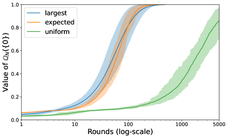
(a) Fixed learning rate $k=4$.

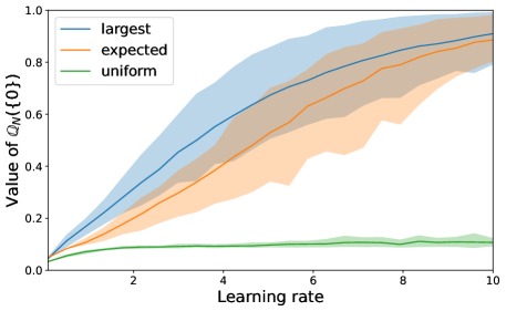
(b) Fixed number of rounds $N=50$.

Figure 2: Convergence of the Gibbs measure in the one-period setting.

Gibbs measure value for the agent’s true risk-aversion at each round of the learning algorithm when selecting the next environment fully at random (”uniform”), according to (4.12) (”largest”), or according to (4.13) (”expected”), while varying the number of rounds (top) and the learning rate $k$ (bottom). Expectation, 10% and 90% quantiles are estimated over 25 runs.

We now take a closer look at the choice of $G_{n}$ during the learning algorithm for the different environment-design methods. We display the evolution of $G_{n}$ at every round $n$ for a specific run in Figures 3(a) and 3(b), where each point corresponds to one of the many environments the learner may choose from. It is interesting to note the exploration-exploitation pattern (see e.g. [38]) with the environment design approaches that are not uniform. It seems as the learner explores different environments at the beginning of the learning phase, and then focuses on a small subset of the available environments to refine its estimation of the agent’s risk aversion. There is some variability seen in Figures 3(a) and 3(b). Indeed, for the environment design approach according to (4.12), the algorithm constantly alternates between two environments, because the second largest value of the Gibbs measure changes at each round, as illustrated in Figure 3(c). As well, for the environment design approach according to (4.13), the exploration pattern reappears once the Gibbs measure attributes most of the weight on a single value. In Figures 3(c) and 3(d), we observe the Gibbs measure values $\mathbb{Q}_{N}$ for all risk aversion candidates in $\Upsilon$ for a specific run, which shows that $\mathbb{Q}_{N}(\ell)$ converges to zero for all $\ell\in\{1,\ldots,L\}$. The legends in these plots give the closest risk-aversion candidates to the agent’s risk aversion $(C_{0},\kappa_{0},\gamma_{0})$. Figure 4 shows similar behaviors when using a larger learning rate of $k=10$.

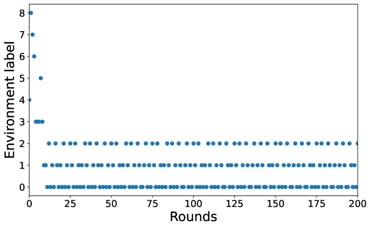
(a) According to (4.12).

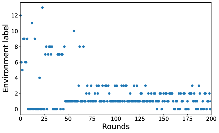
(b) According to (4.13).

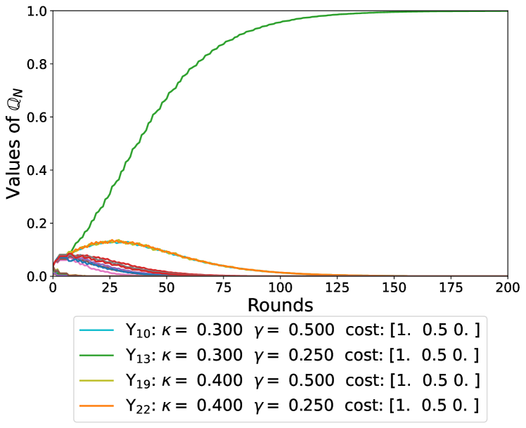
(c) According to (4.12).

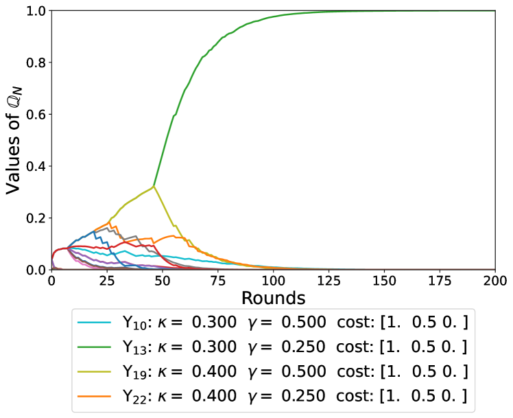
(d) According to (4.13).

Figure 3: Evolution of the designed game and Gibbs measure in the one-period setting for $k=4$.

Evolution of the selected environments at each round of the learning algorithm (top), where each point represents the label of the chosen transition probability matrix characterizing the environment, and evolution of the Gibbs measure at each round of the learning algorithm (bottom), where each line corresponds to one of the many risk-aversion candidates.

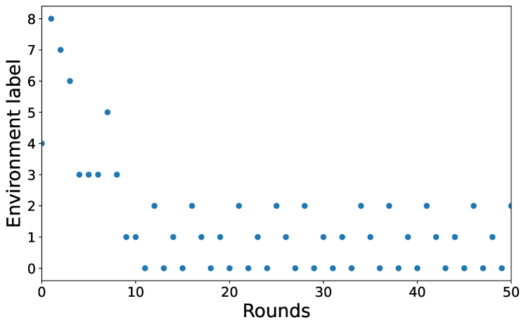
(a) According to (4.12).

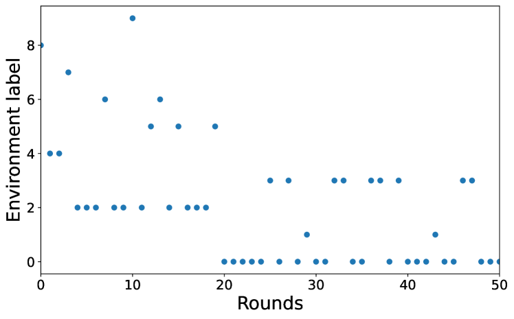
(b) According to (4.13).

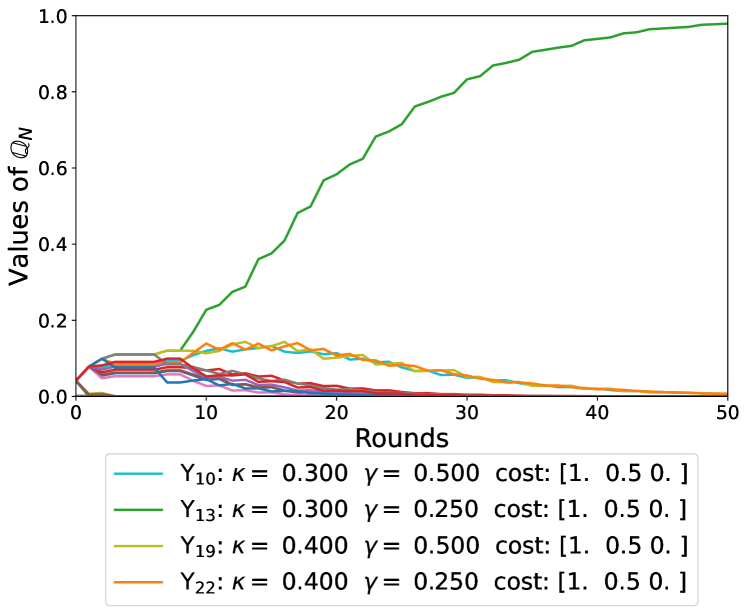
(c) According to (4.12).

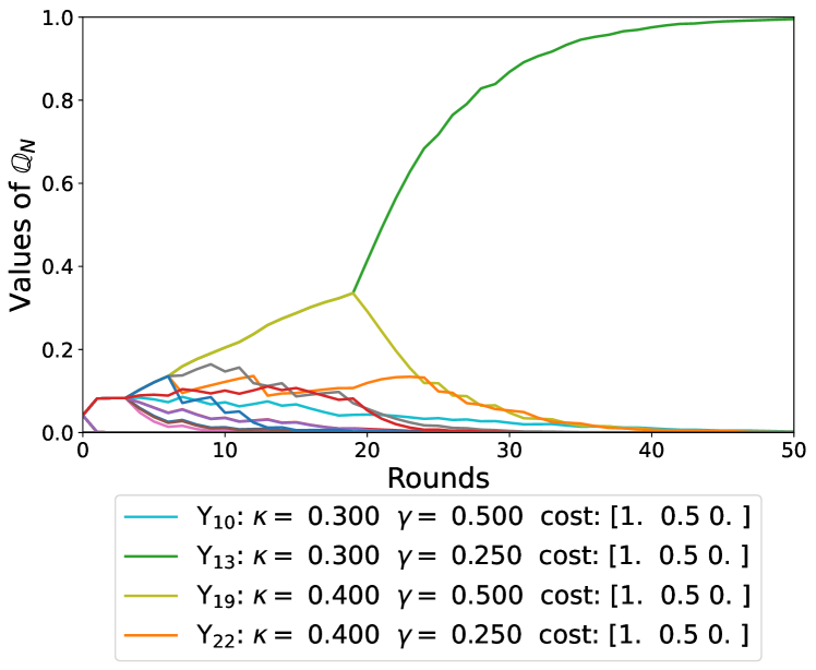
(d) According to (4.13).

Figure 4: Evolution of the designed game and Gibbs measure in the one-period setting for $k=10$.

Evolution of the selected environments at each round of the learning algorithm (top), where each point represents the label of the chosen transition probability matrix characterizing the environment, and evolution of the Gibbs measure at each round of the learning algorithm (bottom), where each line corresponds to one of the many risk-aversion candidates.

An interesting question to ask is: what happens if the true risk aversion of the agent is not in the set of candidates $\Upsilon$ of the learner? In other words, what happens if the model is misspecified? To illustrate this scenario, we now fix the cost function $C_{0}(\mathbb{X})=[1.0,0.5,0.0]$ as well as $\gamma_{0}=0$, but vary the $\kappa$ parameter. More precisely, we take 21 evenly spaced numbers over the interval $[0.1,0.9]$ and set the true parameters $\kappa_{0}$ to 0.24, which does not belong to the set of risk aversion candidates. Figure 5 shows the evolution of the Gibbs measure for the different environment design approaches. When the agent’s true risk aversion is not part of the set of risk candidates $\Upsilon$, the algorithm struggles to choose the truth at the beginning, but eventually converges to the closest risk aversion available. On the other hand, uniformly sampling environments on $\mathcal{P}(\mathbb{X})^{\mathbb{A}}$ fails to decide on the agent’s risk aversion, which is in line with Proposition 4.2. This indicates that a learner may prefer the environment design method according to (4.13) for better identifying the agent’s risk aversion in settings where there is misspecification.

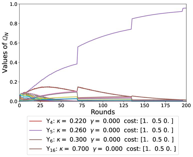
(a) According to (4.12).

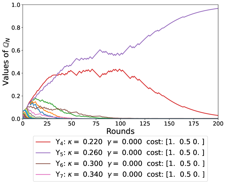
(b) According to (4.13).

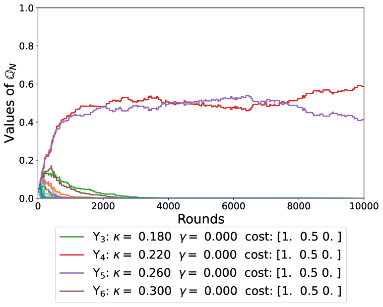
(c) Fully at random.

Figure 5: Evolution of the Gibbs measure for all risk-aversion candidates in the one-period setting.

Evolution of the selected environments at each round of the learning algorithm for different environment-design approaches, where each line corresponds to one of the many risk-aversion candidates. The expert’s true risk-aversion does not belong to the risk-aversion candidates $\Upsilon$.

Infinite horizon case.

We repeat experiments in the infinite horizon setting. Similarly to the one-period setting, we aim to quantify the gain of using environment design approaches according to (4.16) or (4.17) as opposed to random sampling.

In an analogous manner to the one-period case previously described, we suppose that $|\mathbb{X}|=3$, $|\mathbb{A}|=2$, and $C_{\ell}$ satisfies a one-to-one property. For each of the 25 runs, we fix a set of 500 controlled transition matrices ${\widetilde{G}}_{n}\in\mathcal{T}(\mathbb{X})^{\mathbb{A}}$, representing the environments from which the learner can choose, and let the learner interact with the agent for a certain number of rounds to find the agent’s risk-aversion. We set the learning parameter of the Gibbs measure in (4.9) to $k=4$. In addition to the risk measure characterized by $(\kappa,\gamma)$ and the cost function $C$, the learner attempts to also learn the agent’s discount factor $r\in[0,1)$. Therefore, the finite set of risk aversion candidates $\Xi$ is a collection of tuples of the form $(C_{\ell},\kappa_{\ell},\gamma_{\ell},r_{\ell})$. In our experiments, this set contains 36 tuples by taking the Cartesian product between two distinct cost functions, three different $\kappa$’s, two different $\gamma$’s, and three different $r$’s, more specifically

$$\kappa \in\{0.2,0.3,0.4\};$$

$$\gamma \in\{0.2,0.5\};$$

$$r \in\{0.2,0.4,0.6\};$$

$$C(\mathbb{X}) \in\Big{\{}[1.0,0.5,0.0],\;[0.5,1.0,0.0]\Big{\}}.$$

The expert’s risk aversion is given by $\kappa_{0}=0.4$, $\gamma_{0}=0.2$, $r_{0}=0.4$, and $C_{0}(\mathbb{X})=[1.0,0.5,0.0]$.

Since both $\mathbb{X}$ and $\mathbb{A}$ are finite, the challenge of the optimization problem in the infinite-horizon setting lies in the handling of the dynamic programming equation $V$. Indeed, both the regret $\widetilde{\Phi}$ in (4.8) and the distinguishing power $\widetilde{\Psi}$ in (4.14) involve the optimal value function $V^{*}_{\widetilde{G},\ell}$ in (2.8). We suggest to make use of fixed-point iteration to solve this Bellman equation. More precisely, we perform a value iteration algorithm [38, Section 4.4], which finds the optimal $V^{*}$ in (2.7) for each state $x\in\mathbb{X}$. We terminate the value iteration procedure once the value function changes by less than $1\times 10^{-6}$ between two iterations. Note that we compute the optimal value function prior to the learning phase for fixed sets of environments $\widetilde{G}$ and risk aversion candidates $\Xi$.

Once again, carefully designing the next environments provides a much faster convergence than simply randomly sampling one of the available controlled transition matrices, as illustrated in Figure 6(a). We note that learning in the infinite-horizon setting is slower than the one-period setting. This is to be expected, because the learner must discover the discount factor in addition to the cost function and the risk aversion characterization. We also remark that both environment-design approaches are similar in terms of convergence, but (4.13) outperforms (4.12) in terms of variance. At the early stage of the learning process, the agent’s risk aversion may not belong to the largest probabilities assigned by $\widetilde{\mathbb{Q}}_{N}$, which weakens the distinguishing power of (4.12). We believe that both the infinite-horizon setup and the large number of risk aversion candidates emphasize this observation. As remarked in the one-period case, appropriately tuning the learning rate $k$ of the Gibbs measure provides faster convergence. Indeed, Figure 6(b) shows that the learner may faster achieve strong confidence in the agent’s true risk aversion by using larger learning rates.

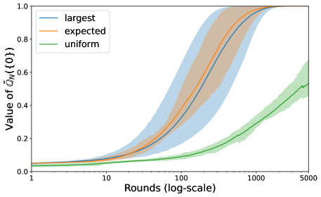
(a) Fixed learning rate $k=4$.

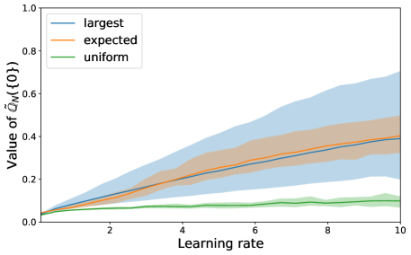
(b) Fixed number of rounds $N=50$.

Figure 6: Convergence of the Gibbs measure in the infinite-horizon setting.

Gibbs measure value for the agent’s true risk-aversion at each round of the learning algorithm when selecting the next environment fully at random (”uniform”), according to (4.12) (”largest”), or according to (4.13) (”expected”), while varying the number of rounds (top) and the learning rate $k$ (bottom). Expectation, 10% and 90% quantiles are estimated over 25 runs.

6 Further discussion on potential further works

In this section, we provide some discussions on potential further works.

6.1 Multiple choices may improve learning

A natural follow-up to Theorem 3.2 is to question whether there exists a scenario where the agent’s risk aversion can be distinguished with only one demonstration. Proposition 6.1 below demonstrates that under the canonical setup described in Remark 2.2, this is possible, provided the state and action space is large enough. The proof is provided in Appendix A.4. However, it remains an open question whether there exists an environment that distinguishes risk aversion with a single demonstration in other settings. The corresponding design problem may also be of interest.

Proposition 6.1.

Consider $\Upsilon=\{\mu_{1},\dots,\mu_{L}\}$. Suppose the canonical setup introduced in Remark 2.2 holds. Then, there exists a state space $\mathbb{X}=\{x_{0},\dots,x_{2L}\}$ with $x_{0}<x_{1}<\dots<x_{2L}$, an action space $\mathbb{A}$ with $|\mathbb{A}|=L$, and an environment $G\in\mathcal{P}(\mathbb{X})^{\mathbb{A}}$ such that

$$\{a_{\ell}\}=\operatorname*{arg\,min}_{a\in\mathbb{A}}\rho_{\mu_{\ell}}\left(X^{a}_{G}\right),\quad\ell=1,\dots,L,$$

where $X^{a}_{G}\sim G$.

6.2 Action-depending cost and design with limited influence

In MDP, the cost function often depends not only on the state but also on the agent’s action. Exploring the identifiability with a cost function depending on both the state and the action is a desirable avenue of research. In addition to a cost function of state and action, it is also important to consider scenarios where the learner has limited influence over the environment, rather than total control. This concern naturally arises in situations such as the imitation of safe driving, where the movement of cars, as characterized by the transition kernel, on the road should obey physical laws.

For the sake of unification, we may consider an environment design problem in infinite horizon with a cost function of the state only and assume the learner has limited influence on the environment. Such a framework can handle a cost function of state and action by augmenting the state space with an artificial buffer that records the state-action of the previous epochs and imposing the design constraint accordingly. A specific state would then be reachable only by selecting the corresponding actions at the corresponding states. For an illustrative example, consider a driving scenario. It is natural to factor in the gas consumption of a maneuver, leading to an action-dependent cost function. Alternatively, we could augment the state space to keep track of the total amount of gas consumed, thereby allowing for a cost function of the state.

6.3 A Bayesian framework

The following Bayesian framework for IRL is a reasonable alternative (cf. [9]) to approach we take. One reason to adopt the Bayesian framework is that it naturally takes into account sub-optimality, as illustrated below. Assume that the agent, given risk aversion $\ell$, chooses action $a$ with probability

$$\frac{h(V(a,\ell,G))}{\sum_{i\in\mathbb{A}}h(V(i,\ell,G))},$$

where $h:\mathbb{R}\to(0,\infty)$ is nonincreasing. Suppose additionally that the choices are independent across different rounds. After $N$ rounds of interactions, under the Bayesian paradigm that

$$\text{posterior}\propto\text{likelihood}\times\text{prior},$$

with uniform prior, the posterior $Q_{N}$ satisfies

$$Q_{N}(\{\ell\})\propto\prod_{n=1}^{N}\frac{h(V(a_{n}^{*},\ell,G_{n}))}{\sum_{i\in\mathbb{A}}h(V(i,\ell,G_{n}))}.$$

It is possible to consider $h$ unknown and integrate the estimation of $h$ as a part of the IRL. It would be interesting to study the identifiability and the convergence of posterior distributions under this setting.

6.4 Function approximation

Instead of using a brute force approach to compute the value function $V$ in the infinite-horizon setting, another approach consists of using neural network as function approximators of $V$. Using neural networks helps mitigate the cost of computing the regret and power, as defined in (4.8) and (4.14), respectively, for the learner every time a new environment $G$ appears. This ultimately becomes important when the action space $\mathbb{A}$ and/or state space $\mathbb{X}$ are continuous. Neural network structures are also known to be universal approximators (see e.g. [28]) which allows the estimation of $V$ to any arbitrary accuracy given a sufficiently large neural net.

One may consider a neural net, denoted $V^{\theta}$, parametrized by some parameters $\theta$ that takes as inputs a risk aversion characterization $\mu_{\ell}$, a discount factor $r_{\ell}$, values of the cost function $C_{\ell}$ as well as an environment $G$, and outputs $V(a,\ell,G)$ for all actions $a\in\mathbb{A}$. Depending on the class of dynamic risk measures under study, the neural network may be trained with a nested simulation framework to approximate general risk aversion characterizations under coherent risk measures (see e.g. [39]). Alternatively, one could focus on elicitable dynamic risk measures (see e.g. [16, 21]), such as subclasses of spectral and distortion risk measures, and make use of strictly consistent scoring functions to efficiently approximate the dynamic risk without any nested simulation. We leave as future work a formal validation of this methodology for continuous states with function approximators.

7 Concluding Remarks

In this paper, we propose an IRL framework for eliciting an agent’s risk preferences in a interactive manner in both one-period and infinite horizon cases. Our algorithm uses a Gibbs measure to assess our confidence on the candidate risk aversion. In both cases, we prove the existence of a distinguishing environment for any two risk aversions, and show that the Gibbs measure concentrates on the agent’s true risk aversion when using a randomly designed environments. In addition, we provide two other approaches for updating the game that results in faster convergence than choosing the games uniformly. We showcase the empirical efficiency of such methods in many settings and illustrate how they outperform a fully random design.

Appendix A Proofs

A.1 Proof of Theorem 3.2

If $C$ and $C^{\prime}$ lead to different preferential orders, we can easily construct a distinguishing environment by considering the form that different actions deterministically lead to different states. Therefore, in what follows, without loss of generality, we assume $C$ and $C^{\prime}$ share the same preferential orders. That is, $0=C(x_{0})<C(x_{1})<\dots<C(x_{d})=1$ and $0=C^{\prime}(x_{0})<C^{\prime}(x_{1})<\dots<C^{\prime}(x_{d})=1$, where $d=|\mathbb{X}|-1$.

It is sufficient to prove the case of $|\mathbb{X}|=3$ and $|\mathbb{A}|=2$. Indeed, once Theorem 3.2 for $|\mathbb{X}|=3$ and $|\mathbb{A}|=2$ is proved, for $|\mathbb{X}|>3$, since $(P^{a})_{a\in\mathbb{A}}$ is free to choose, we can always reduce the environment to $3$ states by assigning $0$ probability to certain states. Moreover, we can reduce the effective number of choices of action by having the same outcome for different actions. The three chosen states would be $x_{0},x_{i},x_{d}$, where $0<i<d$ and $C(x_{i})\neq C^{\prime}(x_{i})$.

For the remainder of the section, we assume $\mathbb{X}=\{x_{0},x_{1},x_{2}\}$ and $\mathbb{A}=\{1,2\}$, with $0=C(x_{0})<C(x_{1})<C(x_{2})=1$ and $0=C^{\prime}(x_{0})<C^{\prime}(x_{1})<C^{\prime}(x_{2})=1$. For notational simplicity, we set $C(x_{1})=c$ and $C^{\prime}(x_{1})=c^{\prime}$. Note that if $c=c^{\prime}$, we must have $\mu\neq\mu^{\prime}$. For $p,q\in[0,1]$, we consider environments $G_{p,q}$ of the form

$$G_{p,q}=\bordermatrix{~{}&1&2\cr x_{0}&1-p&1-q\cr x_{1}&p&0\cr x_{2}&0&q\cr}$$

In view of Lemma 2.1, we define

$$h_{C,\mu}^{1}(p):=\rho_{\mu}(C(X^{1}_{p}))=c\int_{1-p}^{1}\sigma_{\mu}(\kappa)\operatorname{d\!}\kappa\quad\text{and}\quad h_{C,\mu}^{2}(q):=\rho_{\mu}(C(X^{2}_{q}))=c^{-1}h_{C,\mu}^{1}(q),$$ (A.1)

where $X^{1}_{p}\sim(1-p)\delta_{x_{0}}+p\delta_{x_{1}}$ and $X^{2}_{q}\sim(1-q)\delta_{x_{0}}+q\delta_{x_{2}}$. Clearly, $h^{1}_{C,\mu}(1)=c$ and $h^{2}_{C,\mu}(1)=1$. Moreover, both $h_{C,\mu}^{1}$ and $h_{C,\mu}^{2}$ are continuous, nondecreasing and concave due to Lemma 2.1. Let

$$r_{\mu}:=\sup\left\{r\in\mathbb{R}:\int_{r}^{1}\sigma_{\mu}(t)\operatorname{d\!}t=1\right\}.$$ (A.2)

Note that both $h^{1}_{C,\mu}$ and $h^{2}_{C,\mu}$ are strictly increasing in $[0,1-r_{\mu})$, and constant in $[1-r_{\mu},1]$. For $p\in[0,1]$, we further define

$$g_{C,\mu}(p):=\inf\big{\{}q\in[0,1]:h_{C,\mu}^{2}(q)\geq h_{C,\mu}^{1}(p)\big{\}}=\inf\big{\{}q\in[0,1]:h_{C,\mu}^{2}(q)\geq ch_{C,\mu}^{2}(p)\big{\}},$$ (A.3)

where the second equality follows from (A.1). The lemma below provides some useful properties of $g_{C,\mu}$.

Lemma A.1.

The following is true:

• $h_{C,\mu}^{2}(g_{C,\mu}(p))=ch_{C,\mu}^{2}(p)$ for $q\in[0,1]$;

• For $p\in[0,1]$, if $q<g_{C,\mu}(p)$ (resp. $q>g_{C,\mu}(p)$), then $h_{C,\mu}^{2}(q)<h_{C,\mu}^{1}(p)$ (resp. $h_{C,\mu}^{2}(q)>h^{1}_{C,\mu}(p)$);

• $g_{C,\mu}$ is strictly increasing in $[0,1-r_{\mu})$, and constant in $[1-r_{\mu},1]$;

• $g_{C,\mu}$ is continuous in $[0,1]$;

• $g_{C,\mu}(q)=0$ only at $q=0$, $g_{C,\mu}(p)<p$ for $q\in(0,1)$, and $g_{C,\mu}(1)=\inf\{p\in[0,1]:h^{2}_{C,\mu}(p)\geq c\}<1-r_{\mu}$.

Proof.

(a) In view of (A.1), invoking the continuity of $h^{2}_{C,\mu}$, the statement follows immediately.
(b) In view of (A.1), since $h^{1}_{C,\mu}$ is nondecreasing and thus $h^{1}_{C,\mu}(p)\leq h^{1}_{C,\mu}(1)=c$. It follows that

$$g_{C,\mu}(p)\leq\inf\{q\in[0,1]:h^{2}_{C,\mu}(q)\geq c\}=\inf\bigg{\{}q\in[0,1]:\int_{1-q}^{1}\sigma_{\mu}(\kappa)\operatorname{d\!}\kappa\geq c\bigg{\}}<1-r_{\mu},$$ (A.4)

where the last inequality is indeed strict; otherwise, following from statement (a) and (A.2), we have the contradiction below

$$c=h_{C,\mu}^{2}(g_{C,\mu}(1))=h_{C,\mu}^{2}(1-r_{\mu})=h_{C,\mu}^{2}(1)=1$$

In view of the strict monotonicity of $h^{2}_{C,\mu}$ in $[0,1-r_{\mu})$ and (a), the proof is complete.
(c) By (A.2), $h^{2}_{C,\mu}$ is constant in $[1-r_{\mu},1]$. Thus, by (A.3), $g_{C,\mu}$ must also be constant in $[1-r_{\mu},1]$. Regarding the strict monotonicity of $g_{C,\mu}$ in $[0,1-r_{\mu})$, we proceed by contradiction. Suppose there is $0\leq p<p^{\prime}<1-r_{\mu}$ such that $g_{C,\mu}(p)\geq g_{C,\mu}(p^{\prime})$, then by (a) we have

$$ch^{2}_{C,\mu}(p)=h^{2}_{C,\mu}(g_{C,\mu}(p))\geq h^{2}_{C,\mu}(g_{C,\mu}(p^{\prime}))=ch^{2}_{C,\mu}(p^{\prime}),$$

which contradicts the fact that $h^{2}_{C,\mu}$ is strictly increasing in $[0,1-r_{\mu})$ due to (A.2).
(d) Let $(q_{n})_{n\in\mathbb{N}}\subset[0,1]$ converge to $q_{0}$. Then, by statement (a) and the continuity of $h^{2}_{C,\mu}$ due to (A.1), we have

$$h_{C,\mu}^{2}(g_{C,\mu}(q_{n}))=ch^{2}_{C,\mu}(q_{n})\xrightarrow[n\to\infty]{}ch_{C,\mu}^{2}(q_{0}).$$

Note the limit above remains true if we replace $(q_{n})_{n\in\mathbb{N}}$ with a subsequence of $(q_{n})_{n\in\mathbb{N}}$. Replacing $(q_{n})_{n\in\mathbb{N}}$ with its subsequences approximating $\liminf_{n\to\infty}g_{C,\mu}(q_{n})$ and $\limsup_{n\to\infty}g_{C,\mu}(q_{n})$, respectively, we yield

$$h_{C,\mu}^{2}\left(\liminf_{n\to\infty}g_{C,\mu}(q_{n})\right)=h_{C,\mu}^{2}\left(\limsup_{n\to\infty}g_{C,\mu}(q_{n})\right)=ch_{C,\mu}^{2}(q_{0})=h_{C,\mu}^{2}(g_{C,\mu}(q_{0})),$$

where we use statement (a) again in the last equality. Finally, by statement (b), we must have

$$\liminf_{n\to\infty}g_{C,\mu}(q_{n})=\limsup_{n\to\infty}g_{C,\mu}(q_{n})=g_{C,\mu}(q_{0}),$$

which completes the proof.
(e) It is clear from (A.1) and (A.3) that $g_{C,\mu}(0)=0$. The last statement was proved in (A.4). The above together with the monotonicity of $g_{C,\mu}$ implies that $g_{C,\mu}(p)\in(0,1-r_{\mu})$ for $p\in(0,1)$. The second statement follows immediately from statement (a) and (c). ∎

The following lemma is crucial for the construction of a distinguishing environment.

Lemma A.2.

If $(C,\mu)$ and $(C^{\prime},\mu^{\prime})$ are different, then there is $p\in(0,1)$ such that $g_{C,\mu}(p)\neq g_{C^{\prime},\mu^{\prime}}(p)$.

Proof.

Recall that $(C,\mu)$ and $(C^{\prime},\mu^{\prime})$ are different if $c\neq c^{\prime}$ and/or $\mu\neq\mu^{\prime}$. We will prove by contradiction in two different cases. In both cases, we suppose $g_{C,\mu}(p)=g_{C^{\prime},\mu^{\prime}}(p)$ for all $p\in[0,1]$.
Step 1. We first consider the case where $c\neq c^{\prime}$, while $\mu$ and $\mu^{\prime}$ may or may not be different. Without loss of generality, we assume $c<c^{\prime}$. We define $p_{1}=1$ and $p_{k+1}=g_{C,\mu}(p_{k})$ for $k\in\mathbb{N}$. It follows from Lemma A.1 (e) that $(p_{k})_{k\in\mathbb{N}}$ is positive and strictly decreasing. Moreover, $h^{2}_{C,\mu}(p_{1})=1$ by (A.1) and Lemma 2.1, and thus $h^{2}_{C,\mu}(p_{k})=c^{k-1}$ for $k\in\mathbb{N}$ by Lemma A.1 (a). Similarly, $h^{2}_{C^{\prime},\mu^{\prime}}(p_{k})={c^{\prime}}^{k-1}$ for $k\in\mathbb{N}$. It follows that

$$\frac{h^{2}_{C^{\prime},\mu^{\prime}}(p_{k})-h^{2}_{C^{\prime},\mu^{\prime}}(p_{k+1})}{p_{k}-p_{k+1}}=\frac{{c^{\prime}}^{k-1}-{c^{\prime}}^{k}}{p_{k}-p_{k+1}}=\frac{{c^{\prime}}^{k-1}-{c^{\prime}}^{k}}{{c^{\prime}}^{k-1}-{c^{\prime}}^{k-1}c}\frac{{c^{\prime}}^{k-1}}{{c}^{k-1}}\frac{{c}^{k-1}-{c}^{k}}{p_{k}-p_{k+1}}=\frac{1-c^{\prime}}{1-c}\frac{{c^{\prime}}^{k-1}}{{c}^{k-1}}\frac{h^{2}_{C,\mu}(p_{k})-h^{2}_{C,\mu}(p_{k+1})}{p_{k}-p_{k+1}}.$$

For $k\geq 3$, we have $p_{k+1}<p_{k}<p_{2}<p_{1}=1$. We continue to the concavity of $h^{2}_{C^{\prime},\mu^{\prime}}$ and yield

$$\frac{h^{2}_{C^{\prime},\mu^{\prime}}(p_{k})-h^{2}_{C^{\prime},\mu^{\prime}}(p_{k+1})}{p_{k}-p_{k+1}}\geq\frac{1-c^{\prime}}{1-c}\frac{{c^{\prime}}^{k-1}}{{c}^{k-1}}\frac{h^{2}_{C,\mu}(p_{1})-h^{2}_{C,\mu}(p_{2})}{p_{1}-p_{2}}=\frac{{c^{\prime}}^{k-1}}{{c}^{k-1}}\frac{1-c^{\prime}}{p_{1}-p_{2}}.$$

In view of (A.1) and the regularity of $\sigma_{\mu}$ in Lemma 2.1, we must have $\lim_{r\to 1}\sigma_{\mu^{\prime}}(r)=\infty$, contradicting Assumption 3.1 (ii).
Step 2. We now suppose $c=c^{\prime}$, but $\mu\neq\mu^{\prime}$. We define $p_{1}=1$ and $p_{k+1}=g_{C,\mu}(p_{k})$ for $n\in\mathbb{N}$. Similarly as before, $(p_{k})_{k\in\mathbb{N}}$ is positive and strictly decreasing. Additionally, $h^{2}_{C,\mu}(p_{k})=h^{2}_{C,\mu^{\prime}}(p_{k})=c^{k-1}$. We must have $\lim_{k\to\infty}p_{k}=0$; otherwise by Lemma A.1 (d), we have $g_{C,\mu}(p)=0$ for some $p>0$, contradicting (e).

There must be a $\hat{p}\in(0,1)$ such that $h^{2}_{C,\mu}(\hat{p})\neq h^{2}_{C,\mu^{\prime}}(\hat{p})$. Suppose otherwise, then by (A.1) and the right continuity of $\sigma_{\mu},\sigma_{\mu^{\prime}}$ from Lemma 2.1, we have $\sigma_{\mu}=\sigma_{\mu^{\prime}}$. By Lemma 2.1 again, we have $\mu([0,\alpha])=\mu^{\prime}([0,\alpha])$ for $\alpha\in[0,1)$. If follows from monotone class lemma ([4, Section 4.4, Lemma 4.13]) that $\mu=\mu^{\prime}$.

We define $\hat{c}:=h^{2}_{C,\mu}(\hat{p})$ and $\hat{c}^{\prime}:=h^{2}_{C,\mu^{\prime}}(\hat{p})$. Without loss of generality, we assume that $\hat{c}<\hat{c}^{\prime}$. Moreover, since $(p_{k})_{k\in\mathbb{N}}$ is strictly decreasing and $\lim_{k\to\infty}p_{k}=0$, we have $\hat{p}\in(p_{k_{0}+1},p_{k_{0}})$ for some $k_{0}\in\mathbb{N}$. Note that

$$c^{k_{0}}<\hat{c}<\hat{c}^{\prime}<c^{k_{0}-1}$$ (A.5)

We let $\bar{p}_{k}:=p_{k_{0}+k-1}$ for $k\in\mathbb{N}$. Additionally, we define $\hat{p}_{1}:=\hat{p}$ and $\hat{p}_{k+1}=g_{C,\mu}(\hat{p}_{k})$ for $k\in\mathbb{N}$. By Lemma A.1 (a), we have $h^{2}_{C,\mu}(\hat{p}_{k})=c^{k-1}\hat{c}$. The above together with Lemma A.1 (a) implies

$$h^{2}_{C,\mu^{\prime}}(\bar{p}_{k})=h^{2}_{C,\mu^{\prime}}(\bar{p}_{k})=c^{k_{0}+k-2},\quad h^{2}_{C,\mu}(\hat{q}_{k})=\hat{c}c^{k-1},\quad h^{2}_{C,\mu^{\prime}}(\hat{q}_{k})=\hat{c}^{\prime}c^{k-1}.$$ (A.6)

By combining (A.5), (A.6) and the monotonicity of $h^{2}_{C,\mu}$ from definition (A.1), we have

$$\hat{p}_{k+1}<\bar{p}_{k+1}<\hat{p}_{k}<\bar{p}_{k}.$$ (A.7)

It follows from (A.7), the concavities of $h^{2}_{C,\mu^{\prime}}$ from definition (A.1), and (A.6) that

$$\frac{h^{2}_{C,\mu^{\prime}}(\bar{p}_{k+1})-h^{2}_{C,\mu^{\prime}}(\hat{p}_{k+1})}{\bar{p}_{k+1}-\hat{p}_{k+1}}\geq\frac{h^{2}_{C,\mu^{\prime}}(\hat{p}_{k})-h^{2}_{C,\mu^{\prime}}(\bar{p}_{k+1})}{\hat{p}_{k}-\bar{p}_{k+1}}=\frac{\hat{c}^{\prime}c^{k-1}-c^{k_{0}+k-1}}{\hat{p}_{k}-\bar{p}_{k+1}}.$$

Recall that $\hat{c}<\hat{c}^{\prime}$. By (A.6), (A.7) and the the concavities of $h^{2}_{C,\mu}$ in (A.1), we yield

$$\frac{h^{2}_{C,\mu^{\prime}}(\bar{p}_{k+1})-h^{2}_{C,\mu^{\prime}}(\hat{p}_{k+1})}{\bar{p}_{k+1}-\hat{p}_{k+1}}\geq\frac{\hat{c}c^{k-1}-c^{k_{0}+k-1}}{\hat{p}_{k}-\bar{p}_{k+1}}=\frac{h^{2}_{C,\mu}(\hat{p}_{k})-h^{2}_{C,\mu}(\bar{p}_{k+1})}{\hat{p}_{k}-\bar{p}_{k+1}}\geq\frac{h^{2}_{C,\mu}(\bar{p}_{k})-h^{2}_{C,\mu}(\hat{p}_{k})}{\bar{p}_{k}-\hat{p}_{k}}$$

$$\quad=\frac{c^{k_{0}+k-2}-\hat{c}c^{k-1}}{\bar{q}_{k}-\hat{q}_{k}}=\frac{c^{k_{0}-1}-\hat{c}}{c^{k_{0}-1}-\hat{c}^{\prime}}\frac{c^{k_{0}+k-2}-\hat{c}^{\prime}c^{k-1}}{\bar{q}_{k}-\hat{q}_{k}}=\frac{c^{k_{0}-1}-\hat{c}}{c^{k_{0}-1}-\hat{c}^{\prime}}\frac{h^{2}_{C,\mu^{\prime}}(\bar{q}_{k})-h^{2}_{C,\mu^{\prime}}(\hat{q}_{k})}{\bar{q}_{k}-\hat{q}_{k}}.$$

By induction, we have

$$\frac{h^{2}_{C,\mu^{\prime}}(\bar{q}_{k})-h^{2}_{C,\mu^{\prime}}(\hat{q}_{k})}{\bar{q}_{k}-\hat{q}_{k}}\geq\left(\frac{c^{k_{0}-1}-\hat{c}}{c^{k_{0}-1}-\hat{c}^{\prime}}\right)^{k-1}\frac{h^{2}_{C,\mu^{\prime}}(\bar{q}_{1})-h^{2}_{C,\mu^{\prime}}(\hat{q}_{1})}{\bar{q}_{1}-\hat{q}_{1}}=\left(\frac{c^{k_{0}-1}-\hat{c}}{c^{k_{0}-1}-\hat{c}^{\prime}}\right)^{k-1}\frac{c^{k_{0}-1}-\hat{c}}{\bar{p}_{k_{0}}-\hat{p}},$$

where we note $\frac{c^{k_{0}-1}-\hat{c}}{c^{k_{0}-1}-\hat{c}^{\prime}}>1$ due to (A.5). In view of (A.1) and the regularity of $\sigma_{\mu}$ in Lemma 2.1, we must have $\lim_{r\to 1}\sigma_{\mu^{\prime}}(r)=\infty$, contradicting Assumption 3.1 (ii). ∎

We are ready to prove Theorem 3.2.

Proof of Theorem 3.2.

Let $p$ be defined as in Lemma A.2. Without loss of generality, we assume $g_{C,\mu}(p)<g_{C^{\prime},\mu^{\prime}}(p)$. Pick $q\in(g_{C,\mu}(p),g_{C^{\prime},\mu^{\prime}}(p))$. Then, by Lemma A.1 (b) and (A.1), we have $\rho_{\mu}(C(X^{1}_{G_{p,q}}))<\rho_{\mu}(C(X^{2}_{G_{p,q}}))$, while $\rho_{\mu^{\prime}}(C^{\prime}(X^{1}_{G_{p,q}}))>\rho_{\mu^{\prime}}(C^{\prime}(X^{2}_{G_{p,q}}))$, i.e., $G_{p,q}$ is the distinguishing environment. This completes the proof. ∎

A.2 Proof of Theorem 3.3

We start by establishing a technical lemma.

Lemma A.3.

Suppose an infinite horizon setting where Assumption 3.1 holds. Assume additionally that there is $P^{a}\in\mathcal{P}(\mathbb{X})^{\mathbb{A}}$ such that $T^{a}_{x}=P^{a}$ for all $x\in\mathbb{X}$, and denote $G=(P^{a})_{a\in\mathbb{A}}$. Then, for any $(C,\mu,r)\in\Xi$, we have $\pi^{*}$ is the optimal action if and only if $\pi^{*}(x)\in\operatorname*{arg\,min}_{a}\rho_{\mu}(X^{a}_{G})$ for all $x\in\mathbb{X}$, and and $\varrho^{x,\infty}_{C,\mu,r}(\pi^{*};{\widetilde{G}})=C(x)+r(1-r)^{-1}\min_{a}\rho_{\mu}(X^{a}_{G})$ for $x\in\mathbb{X}$.

Proof.

We first show that $\min_{\pi}\varrho^{x,\infty}_{C,\mu,r}\left(\pi;{\widetilde{G}}\right)\geq C(x)+r(1-r)^{-1}\min_{a}\rho_{\mu}(X^{a}_{G})$ for any $x\in\mathbb{X}$. Recall that $R^{\pi,{\widetilde{G}}}_{C,\mu,r}0(x)=C(x)$ and note that, for any $x\in\mathbb{X}$,

$$R^{\pi,{\widetilde{G}}}_{C,\mu,r}\circ R^{\pi,{\widetilde{G}}}_{C,\mu,r}O(x) =C(x)+r\rho_{\mu}\left(C\left(X^{x,\pi(x)}_{{\widetilde{G}}}\right)\right)$$

$$=C(x)+r\rho_{\mu}\left(C\left(X^{\pi(x)}_{G}\right)\right)\geq C(x)+r\min_{a}\rho_{\mu}(X^{a}_{G})$$ (A.8)

We proceed by backward induction. For $\tau\geq 2$, suppose $\left(R^{\pi,{\widetilde{G}}}_{C,\mu,r}\right)^{\tau}O(x)\geq C(x)+\sum_{t=1}^{\tau-1}r^{t}\min_{a}\rho_{\mu}\left(C\left(X^{a}_{G}\right)\right)$ for $x\in\mathbb{X}$, then

$$(R^{\pi,{\widetilde{G}}}_{C,\mu,r})^{\tau+1}O(x)=C(x)+r\rho_{\mu}\left(\left(R^{\pi,{\widetilde{G}}}_{C,\mu,r}\right)^{\tau}O\left(X^{x,\pi(x)}_{{\widetilde{G}}}\right)\right)=C(x)+r\rho_{\mu}\left(\left(R^{\pi,{\widetilde{G}}}_{C,\mu,r}\right)^{\tau}O\left(X^{\pi(x)}_{G}\right)\right)$$

$$\quad=C(x)+r\rho_{\mu}\left(C\left(X^{\pi(x)}_{G}\right)\right)+r\sum_{t=2}^{\tau-1}r^{t}\min_{a}\rho_{\mu}\left(C\left(X^{a}_{G}\right)\right)\geq C(x)+\sum_{t=1}^{\tau}r^{t}\min_{a}\rho_{\mu}(X^{a}_{G}).$$ (A.9)

Letting $\tau\to\infty$, we show that $\min_{\pi}\varrho^{x,\infty}_{C,\mu,r}\left(\pi;{\widetilde{G}}\right)\geq C(x)+r(1-r)^{-1}\min_{a}\rho_{\mu}\left(X^{a}_{G}\right)$ for any $x\in\mathbb{X}$.

Next, we will argue that if $\pi(x)\in\operatorname*{arg\,min}_{a}\rho_{\mu}(X^{a}_{G})$ for $x\in\mathbb{X}$, then $\varrho^{x,\infty}_{C,\mu,r}(\pi;{\widetilde{G}})$ attains the lower bound. To this end note that the equality in (A.2) is attained for all $x\in\mathbb{X}$ if $\pi\equiv(x)\in\operatorname*{arg\,min}_{a}\rho_{\mu}(X^{a}_{G})$. Inducing backward, we have that such $\pi$ also attains the equality in (A.2).

Lastly, we argue that, in order to attain the optimal, it is necessary for $\pi(x)\in\operatorname*{arg\,min}_{a}\rho_{\mu}(X^{a}_{G})$ for all $x\in\mathbb{X}$. Otherwise, starting the experiment at $x$ where the aforementioned is violated will lead to a strictly suboptimal case

$$\left(R^{\pi,{\widetilde{G}}}_{C,\mu,r}\right)^{\infty}O(x)=C(x)+r\rho_{\mu}\left(\left(R^{\pi,{\widetilde{G}}}_{C,\mu,r}\right)^{\infty}O\left(X^{\pi(x)}_{G}\right)\right)\geq C(x)+r\rho_{\mu}\left(\varrho^{X^{\pi(x)}_{G},\infty}_{C,\mu,r}\left(\pi^{*};{\widetilde{G}}\right)\right)>\varrho^{x,\infty}_{C,\mu,r}\left(\pi^{*};{\widetilde{G}}\right),$$

where we have used (2.7) for the first equality. ∎

Proof of Theorem 3.3.

Without loss of generality, we suppose $C$ and $C^{\prime}$ share common preferential orders. That is, $C(x_{0})\leq C(x_{1})\leq\cdots\leq C(x_{d})$ and $C^{\prime}(x_{0})\leq C^{\prime}(x_{1})\leq\cdots\leq C^{\prime}(x_{d})$, where $d=|\mathbb{X}|$. Indeed, if this is not the case, we can simply design an environment with deterministic actions to distinguish between $C$ and $C^{\prime}$. In a similar manner to Lemma A.2, we consider the different cases that make $(C,\mu,r)$ and $(C^{\prime},\mu^{\prime},r^{\prime})$ distinct.

We first prove the case with $(C,\mu)\neq(C^{\prime},\mu^{\prime})$, while $r$ may or may not be the same as $r^{\prime}$. We construct ${\widetilde{G}}$ in the space homogeneous setting, i.e., there is $P^{a}\in\mathcal{P}(\mathbb{X})$ such that $T^{a}_{x}=P^{a}$ for all $(x,a)\in\mathbb{X}$. By Theorem 3.2, there is $G=(P^{a})_{a\in\mathbb{A}}$ such that

$$\operatorname*{arg\,min}_{a}\rho_{\mu}\left(C(X^{a}_{G})\right)\cap\operatorname*{arg\,min}_{a}\rho_{\mu^{\prime}}\left(C^{\prime}(X^{a}_{G})\right)=\emptyset.$$ (A.10)

In view of Lemma A.3, let $\pi^{*}(x)\in\operatorname*{arg\,min}_{a}\rho_{\mu}\left(C(X^{a}_{G})\right)$ and ${\pi^{*}}^{\prime}(x)\in\operatorname*{arg\,min}_{a}\rho_{\mu^{\prime}}\left(C^{\prime}(X^{a}_{G})\right)$ for $x\in\mathbb{X}$, i.e., $\pi^{*}$ and $(\pi^{*})^{\prime}$ are the optimal policies under $(C,\mu,r)$ and $(C^{\prime},\mu^{\prime},r^{\prime})$, respectively. What is left to show is that both ${\pi^{*}}^{\prime}$ and $\pi^{*}$ are not optimal under $(C,\mu,r)$ and $(C^{\prime},\mu^{\prime},r^{\prime})$, respectively. The following reasoning is similar to the proof of Lemma A.3, and is presented here for the sake of completeness. Let $\mathbb{A}^{*}:=\operatorname*{arg\,min}_{a}\rho_{\mu}\left(C(X^{a}_{G})\right)$. Note that

$$R^{{\pi^{*}}^{\prime},{\widetilde{G}}}_{C,\mu,r}\circ R^{{\pi^{*}}^{\prime},{\widetilde{G}}}_{C,\mu,r}O(x) =C(x)+r\rho_{\mu}\left(C\left(X^{x,{\pi^{*}}^{\prime}(x)}_{{\widetilde{G}}}\right)\right)$$

$$=C(x)+r\rho_{\mu}\left(C\left(X^{{\pi^{*}}^{\prime}(x)}_{G}\right)\right)\geq C^{\prime}(x)+r\min_{a\notin{\mathbb{A}^{*}}}\rho_{\mu}\left(C\left(X^{a}_{G}\right)\right),$$ (A.11)

where the last inequality follows from (A.10). Moreover, $\left(R^{{\pi^{*}}^{\prime},{\widetilde{G}}}_{C,\mu,r}\right)^{\tau}O(x)\geq C(x)+\sum_{t=1}^{\tau-1}{r}^{t}\min_{a\notin{\mathbb{A}^{*}}}\rho_{\mu}(C(X^{a}_{G}))$ for $x\in\mathbb{X}$ and $\tau\geq 2$ implies that

$$\left(R^{{\pi^{*}}^{\prime},{\widetilde{G}}}_{C,\mu,r}\right)^{\tau+1}O(x) =C(x)+r\rho_{\mu}\left(\left(R^{{\pi^{*}}^{\prime},{\widetilde{G}}}_{C,\mu,r}\right)^{\tau}O\left(X^{x,{\pi^{*}}^{\prime}(x)}_{{\widetilde{G}}}\right)\right)=C(x)+r\rho_{\mu}\left(\left(R^{{\pi^{*}}^{\prime},{\widetilde{G}}}_{C,\mu,r}\right)^{\tau}O\left(X^{{\pi^{*}}^{\prime}(x)}_{G}\right)\right)$$

$$=C(x)+r\rho_{\mu}\left(C\left(X^{{\pi^{*}}^{\prime}(x)}_{G}\right)\right)+\sum_{t=2}^{\tau-1}{r}^{t}\min_{a\notin{\mathbb{A}^{*}}}\rho_{\mu}(C(X^{a}_{G}))\geq C(x)+\sum_{t=1}^{\tau}r^{t}\min_{a\notin{\mathbb{A}^{*}}}\rho_{\mu}(X^{a}_{G}).$$

In view of Definition 2.5, letting $\tau\to\infty$, we have

$$\varrho^{x,\infty}_{C,\mu,r}({\pi^{*}}^{\prime};{\widetilde{G}})\geq C(x)+\sum_{t=1}^{\infty}r^{t}\min_{a\notin{\mathbb{A}^{*}}}\rho_{\mu}(X^{a}_{G})>C(x)+\sum_{t=1}^{\infty}r^{t}\min_{a}\rho_{\mu}(X^{a}_{G}),$$

which is not optimal by Lemma A.3. A similar reasoning shows that $\pi^{*}$ is not optimal in $(C^{\prime},\mu^{\prime},r^{\prime})$.

Next, we prove the case with $(C,\mu)=(C^{\prime},\mu^{\prime})$ but $r\neq r^{\prime}$. We can restrict the environment to have $|\mathbb{X}|=3$ by constructing non-transient block. We also assume $|\mathbb{A}|=2$, which can be done by letting additional actions having the exact same outcome as one of the previous actions. Without loss of generality, we also suppose $0=C(x_{0})<C(x_{1})<C(x_{2})=1$. Let ${\widetilde{G}}_{p}:=\left(T^{a}_{p}\right)_{a\in\{1,2\}}$ with

$$T^{1}_{p}:=\bordermatrix{~{}&x_{0}&x_{1}&x_{2}\cr x_{0}&1&0&0\cr x_{1}&p&1-p&0\cr x_{2}&1&0&0\cr}\quad\text{and}\quad T^{2}_{p}:=\bordermatrix{~{}&x_{0}&x_{1}&x_{2}\cr x_{0}&0&0&1\cr x_{1}&0&0&1\cr x_{2}&0&0&1\cr}.$$

It is clear that for $\pi$ to be optimal, it must satisfies $\pi(x_{0})=1$ and $\pi(x_{2})=1$. Let

$$\pi^{1}(x)=\begin{cases}1,&x=x_{0},\\ 1,&x=x_{1},\\ 1,&x=x_{2},\\ \end{cases}\quad\text{and}\quad\pi^{2}(x)=\begin{cases}1,&x=x_{0},\\ 2,&x=x_{1},\\ 1,&x=x_{2}.\\ \end{cases}$$

Clearly, $\varrho^{x_{1},\infty}_{C,\mu,r}\left(\pi^{2};{\widetilde{G}}_{p}\right)=C(x_{1})+r$. In order to compare $\pi^{1}$ and $\pi^{2}$, what is left to compute is $\varrho^{x_{1},\infty}_{C,\mu,r}\left(\pi^{1};{\widetilde{G}}_{p}\right)$. In view of (2.7) and Lemma 2.1, we solve the following for $u\mathbb{R}$

$$u=C(x_{1})+r\rho_{\mu}\left(C\left(X^{x_{1},1}_{{\widetilde{G}}_{p}}\right)\right)=C(x_{1})+ru\int_{1-p}^{1}\sigma_{\mu}(\alpha)\operatorname{d\!}\alpha.$$

Consequently, we yield $\varrho^{x_{1},\infty}_{C,\mu,r}\left(\pi^{1};{\widetilde{G}}_{p}\right)=\left(1-r\int_{1-p}^{1}\sigma_{\mu}(\alpha)\operatorname{d\!}\alpha\right)^{-1}C(x_{1})$. Thus, $\pi^{1}$ is optimal if $p>\overline{p}_{r}$ and $\pi^{2}$ is optimal if $p<\underline{p}_{r}$, where

$$\overline{p}_{r}:=\inf\left\{p\in[0,1]:\frac{C(x_{1})}{1-r\int_{1-p}^{1}\sigma_{\mu}(\alpha)\operatorname{d\!}\alpha}<r\right\}=\inf\left\{p\in[0,1]:\int_{1-p}^{1}\sigma_{\mu}(\alpha)\operatorname{d\!}\alpha<\frac{r}{C(x_{1})+r}\right\},$$

$$\underline{p}_{r}:=\sup\left\{p\in[0,1]:\frac{C(x_{1})}{1-r\int_{1-p}^{1}\sigma_{\mu}(\alpha)\operatorname{d\!}\alpha}>r\right\}=\sup\left\{p\in[0,1]:\int_{1-p}^{1}\sigma_{\mu}(\alpha)\operatorname{d\!}\alpha>\frac{r}{C(x_{1})+r}\right\}.$$

Both $\overline{p}_{r}$ and $\underline{p}_{r}$ are well-defined due to the setting that $C(x_{1})\in(0,1)$ and Lemma 2.1. Without loss of generality, assume $r<r^{\prime}$, and note that $\frac{r^{\prime}}{C(x_{1})+r^{\prime}}<\frac{r}{C(x_{1})+r}$. Since $p\mapsto\int_{1-p}^{1}\sigma_{\mu}(\operatorname{d\!}\alpha)$ is continuous, we have $\overline{p}_{r^{\prime}}<\underline{p}_{r}$. Pick $p\in(\overline{p}_{r^{\prime}},\underline{p}_{r})$, then $\pi^{2}$ is optimal under $(C,\mu,r)$ and $\pi^{1}$ is optimal under $(C,\mu,r^{\prime})$. The proof is complete. ∎

A.3 Proof of Proposition 4.2 and Proposition 4.4

Below we equip $\mathcal{P}(\mathbb{X})^{\mathbb{A}}$ and $\mathbb{R}^{\mathbb{A}}$ with the entrywise $1$-norm. The lemma below regards the continuity of $\Phi$ in $G$.

Lemma A.4.

$G\in\mathcal{P}(\mathbb{X})^{\mathbb{A}}\mapsto\big{(}\Phi(a;G,\ell)\big{)}_{a\in\mathbb{A}}\in\mathbb{R}^{\mathbb{A}}$ is continuous.

Proof.

This is an immediate consequence of (2.5). ∎

We are ready to prove Proposition 4.2.

Proof of Proposition 4.2.

To start with, for $\ell\in\{0,\dots,L\}$, we define an auxiliary random variable

$$\xi_{N}^{\ell}=-\beta\sum_{n=1}^{N}\Phi(\alpha^{*}_{n};\Gamma_{n},\ell).$$

Clearly, $\mathfrak{Q}_{N}$ assigns probability $e^{\xi_{N}^{\ell}}/\sum_{k=0}^{L}e^{\xi_{N}^{k}}$ to $\{\ell\}$. By the nonnegativity of $\Phi$ following (4.1), $(\xi_{N}^{\ell})_{n\in\mathbb{N}}$ is a nonincreasing sequence for any $\ell$, meanwhile $\xi_{N}^{0}=0$ for all $N\in\mathbb{N}$ due to (4.4). In view of Theorem 3.2, for $\ell=1,\dots,L$, we let $H_{\ell}\in\mathcal{P}(\mathbb{X})^{\mathbb{A}}$ be an environment that distinguishes $(C_{0},\mu_{0})$ and $(C_{\ell},\mu_{\ell})$. Consequently, for $\ell=1,\dots,L$, there exists $\varepsilon_{\ell}>0$ such that for any $a^{*}\in\operatorname*{arg\,min}_{a\in\mathbb{A}}\rho_{\mu_{0}}(C_{0}(X^{a}_{H_{\ell}}))$, we have $\Phi(a^{*},H_{\ell},\ell)>\varepsilon_{\ell}$. Then, by Lemma A.4, there exists an open ball on $\mathcal{P}(\mathbb{X})^{\mathbb{A}}$ with radius $\delta_{\ell}>0$ under entrywise $1$-norm, denoted by $B_{\delta_{\ell}}(H_{\ell})$, such that for any $H\in B_{\delta_{\ell}}(H_{\ell})$ and $a^{*}\in\operatorname*{arg\,min}_{a\in\mathbb{A}}V(a,0,H)$, we have $\Phi(a^{*},H,\ell)>\varepsilon_{\ell}/2$. It follows that

$$\xi_{N}^{\ell}\leq-\beta\frac{\varepsilon_{\ell}}{2}\sum_{n=1}^{N}\mathbbm{1}_{B_{\delta_{\ell}}(H_{\ell})\cap\mathcal{P}(\mathbb{X})^{\mathbb{A}}}(G_{n}).$$

Because $M(B_{\delta_{\ell}}(H_{\ell})\times\{a\})>0$, by second Borel-Cantelli lemma, $B_{\delta_{\ell}}(H_{\ell})$ will be visited infinitely often with probability $1$. Consequently, $\mathbb{P}\big{(}\limsup_{N\to\infty}\xi^{\ell}_{N}=-\infty\big{)}=1$ for $\ell\neq 0$, and thus

$$\mathbb{P}\bigg{[}\big{\{}\xi^{0}_{N}=0,N\in\mathbb{N}\big{\}}\cap\bigg{\{}\limsup_{N\to\infty}\xi^{\ell}_{N}=-\infty,\ell=1\dots,L\bigg{\}}\bigg{]}=1,$$

which completes the proof. ∎

The proof of Proposition 4.4 follows the exact structure utilized in the proof for Proposition 4.2. For the sake of completeness, we have included the detailed proof here. We start by establishing the continuity of $\widetilde{G}\in\mathcal{T}(\mathbb{X})^{\mathbb{A}}\mapsto\left(\widetilde{\Phi}(\pi;\widetilde{G},\ell)\right)_{\pi\in\Pi}\in\mathbb{R}^{\Pi}$, where $\mathcal{T}(\mathbb{X})^{\mathbb{A}}$ and $\mathbb{R}^{\Pi}$ are equipped with entrywise $1$-norm for convenience.

Lemma A.5.

For any $(x,\ell)\in\mathbb{X}\times\{0,\dots,L\}$, $\widetilde{G}\in\mathcal{T}(\mathbb{X})^{\mathbb{A}}\mapsto\left(\widetilde{\Phi}(\pi;\widetilde{G},\ell)\right)_{\pi\in\Pi}\in\mathbb{R}^{\Pi}$ is continuous.

Proof.

We first show that for any bounded continuous $V:\mathbb{X}\times\mathcal{T}(\mathbb{X})^{\mathbb{A}}\mapsto\mathbb{R}$,

$$\widetilde{G}\mapsto\rho_{\mu_{\ell}}\left(V\left(X^{x,k}_{\widetilde{G}},\widetilde{G}\right)\right)$$ (A.12)

must be continuous. Indeed, in view of (2.2), for $\kappa\in(0,1]$ we have

$$\operatorname{\mathrm{AV}@\mathrm{R}}_{\kappa}\left(V\left(X^{x,k}_{\widetilde{G}},\widetilde{G}\right)\right)=\inf_{|z|\leq\|V\|_{\infty}}\left\{z+\frac{1}{\kappa}\sum_{y\in\mathbb{X}}\widetilde{G}^{k}_{xy}\left(V\left(y,\widetilde{G}\right)-z\right)_{+}\right\}.$$ (A.13)

It follows that $\widetilde{G}\mapsto\operatorname{\mathrm{AV}@\mathrm{R}}_{\kappa}\left(V\left(X^{x,k}_{\widetilde{G}},\widetilde{G}\right)\right)$ is continuous (cf. [4, Section 17.5, Lemma 17.29 and Lemma 17.30]). This together dominated convergence implies that $\widetilde{G}\mapsto\rho_{\mu_{\ell}}\left(V^{*}_{\widetilde{G},\ell}\left(X^{x,k}_{\widetilde{G}}\right)\right)$ is continuous.

In view of Definition 2.5, invoking (A.12) repeatedly verifies that $\widetilde{G}\mapsto\varrho_{C_{\ell},\mu_{\ell},r_{\ell}}^{x,\tau}(\pi;{\widetilde{G}})$ is continuous. This together with the convergence of $\left(\varrho_{C_{\ell},\mu_{\ell},r_{\ell}}^{x,\tau}\left(\pi;{\widetilde{G}}\right)\right)_{\tau\in\mathbb{N}}$ implies that $\widetilde{G}\mapsto\varrho_{C_{\ell},\mu_{\ell},r_{\ell}}^{x,\infty}\left(\pi;{\widetilde{G}}\right)$ is continuous. Since the minimum of a finite family of continuous functions is also continuous, in view of (2.11), we have $\widetilde{G}\mapsto V^{*}_{\widetilde{G},\ell}(x)$ is also continuous. Furthermore, since $r_{\ell}\in(0,1)$, we have $\left|V^{*}_{\widetilde{G},\ell}(x)\right|\leq(1-r_{\ell})^{-1}$. This allow us to apply (A.12) to obtain the continuity of $\widetilde{G}\mapsto\rho_{\mu_{\ell}}\left(V^{*}_{\widetilde{G},\ell}\left(X^{x,k}_{\widetilde{G}}\right)\right)$. In view of (4.7) and (4.8), we conclude the proof. ∎

We are ready to prove Proposition 4.4.

Proof of Proposition 4.4.

Similarly to the proof of Proposition 4.2, for $\ell\in\{0,\dots,L\}$, we define an auxiliary random variable

$$\tilde{\xi}_{N}^{\ell}=-\beta\sum_{n=1}^{N}\widetilde{\Phi}\left(\varpi^{*}_{n};\widetilde{\Gamma}_{n},\ell\right).$$

Note that $\widetilde{\mathfrak{Q}}_{N}$ assigns probability $e^{\tilde{\xi}_{N}^{\ell}}/\sum_{k=0}^{L}e^{\tilde{\xi}_{N}^{k}}$ to $\{\ell\}$. By the nonnegativity of $\widetilde{\Phi}$ following (4.8), $\big{(}\tilde{\xi}_{N}^{\ell}\big{)}_{n\in\mathbb{N}}$ is a nonincreasing sequence for any $\ell$, meanwhile $\tilde{\xi}_{N}^{0}=0$ for all $N\in\mathbb{N}$ due to (4.4). In view of Theorem 3.3, for $\ell=1,\dots,L$, we let $\widetilde{H}_{\ell}\in\mathcal{T}(\mathbb{X})^{\mathbb{A}}$ be a environment that distinguishes $(C_{0},\mu_{0},r_{0})$ and $(C_{\ell},\mu_{\ell},r_{\ell})$. Consequently, for $\ell=1,\dots,L$, there is $\varepsilon_{\ell}>0$ such that for any $\pi^{*}$ that is optimal under $(C_{0},\mu_{0},r_{0})$, we have $\widetilde{\Phi}(\pi^{*},\widetilde{H}_{\ell},\ell)>\varepsilon_{\ell}$. Then, by Lemma A.5, there is an open ball on $\mathcal{T}(\mathbb{X})^{\mathbb{A}}$ with radius $\delta_{\ell}>0$ under entrywise $1$-norm, denoted by $B_{\delta_{\ell}}\big{(}\widetilde{H}_{\ell}\big{)}$, such that for any $\widetilde{H}\in B_{\delta_{\ell}}\big{(}\widetilde{H}_{\ell}\big{)}$ and $\pi^{*}$ that is optimal under $(C_{0},\mu_{0},r_{0})$, we have $\widetilde{\Phi}\big{(}\pi^{*},\widetilde{H},\ell\big{)}>\varepsilon_{\ell}/2$. It follows that

$$\tilde{\xi}_{N}^{\ell}\leq-\beta\frac{\varepsilon_{\ell}}{2}\sum_{n=1}^{N}\mathbbm{1}_{B_{\delta_{\ell}}(\widetilde{H}_{\ell})\cap\mathcal{T}(\mathbb{X})^{\mathbb{A}}}(G_{n}).$$

Because $\widetilde{M}\left(B_{\delta_{\ell}}\left(\widetilde{H}_{\ell}\right)\times\{a\}\right)>0$, by second Borel-Cantelli lemma, $B_{\delta_{\ell}}(H_{\ell})$ will be visited infinitely often with probability $1$. Consequently, $\mathbb{P}\big{(}\limsup_{N\to\infty}\tilde{\xi}^{\ell}_{N}=-\infty\big{)}=1$ for $\ell\neq 0$, and thus

$$\mathbb{P}\bigg{[}\left\{\tilde{\xi}^{0}_{N}=0,N\in\mathbb{N}\right\}\cap\bigg{\{}\limsup_{N\to\infty}\tilde{\xi}^{\ell}_{N}=-\infty,\ell=1\dots,L\bigg{\}}\bigg{]}=1,$$

which completes the proof. ∎

A.4 Proof of Proposition 6.1

We start by establishing a useful technical lemma.

Lemma A.6.

For $i=1,\dots,L$, let $\sigma_{i}=\sigma_{\mu_{i}}$, where $\sigma_{\mu_{i}}$ is defined in (2.3). If $\mu_{i}\neq\mu_{j}$, then there exist $0\leq c<d<1$ and $0\leq s<t<1$ such that $\sigma_{i}(r)-\sigma_{j}(r)<0$ for $r\in(c,d)$ and $\sigma_{i}(r)-\sigma_{j}(r)>0$ for $r\in(s,t)$, respectively.

Proof.

We will proceed by contradiction. Suppose for any $(s,t)\subseteq[0,1)$, we have $\sigma_{i}(r)-\sigma_{j}(r)\leq 0$ for some $r\in(c,d)$. Consequently, $\{r\in[0,1):\sigma_{i}(r)-\sigma_{j}(r)\leq 0\}$ is dense in $[0,1)$. Combining this with the right continuity in Lemma 2.1, we yield $\sigma_{i}(r)-\sigma_{j}(r)\leq 0$ for $r\in[0,1)$. But since $\int_{0}^{1}\sigma_{i}(r)\operatorname{d\!}r=\int_{0}^{1}\sigma_{j}(r)\operatorname{d\!}r=1$, we must have $\sigma_{i}(r)=\sigma_{j}(r)$ for Lebesgue almost every $r\in[0,1)$, and thus every $r\in[0,1)$ due to right continuity again. This together with Lemma 2.1 and monotone class lemma ([4, Section 4.4, Lemma 4.13]) implies $\mu_{i}=\mu_{j}$, which contradicts the hypothesis that $\mu_{i}\neq\mu_{j}$. Analogously, there must exists $0\leq c<d<1$ such that $\sigma_{i}(r)-\sigma_{j}(r)<0$ for $r\in(c,d)$ as long as $\mu_{i}\neq\mu_{j}$. ∎

We are in position of proving Proposition 6.1.
$\mathbf{L=2}$. Although the statement for $L=2$ can be considered as a special case of Theorem 3.2, we present an alternative proof here in order to better illustrate a key mechanism used in the proof for $L\geq 3$. We select arbitrarily $x_{0}<x_{1}<x_{2}$. In view of Lemma A.6, we let $(c,d)$ and $(s,t)$ be non-empty interval on $[0,1]$ such that

$$\sigma_{1}(r)<\sigma_{2}(r),\,\,r\in(c,d)\quad\text{and}\quad\sigma_{1}(r)>\sigma_{2}(r),\,\,r\in(s,t).$$ (A.14)

Here, we only present the argument for the case of $d\leq s$ as the case of $c\geq t$ can be done analogously. By (A.14), because $\sigma_{i},\,i=1,2$ are non-negative and nondecreasing, we have $\sigma_{2}(r)>0$ for $r>c$. For $\varepsilon\in(0,d-c)$ sufficiently small, there is a $\delta_{0}\in(0,t-s)$ such that

$$(x_{1}-x_{0})\int_{c}^{c+\varepsilon}\sigma_{2}(r)\operatorname{d\!}r=(x_{2}-x_{1})\int_{t-\delta_{0}}^{t}\sigma_{2}(r)\operatorname{d\!}r.$$

By (A.14) again, for the $\varepsilon$ and $\delta$ introduced above, we have

$$(x_{1}-x_{0})\int_{c}^{c+\varepsilon}\!\sigma_{1}(r)\operatorname{d\!}r<(x_{1}-x_{0})\int_{c}^{c+\varepsilon}\sigma_{2}(r)\operatorname{d\!}r\\ =(x_{2}-x_{1})\int_{t-\delta_{0}}^{t}\sigma_{2}(r)\operatorname{d\!}r<(x_{2}-x_{1})\int_{t-\delta_{0}}^{t}\sigma_{1}(r)\operatorname{d\!}r.$$ (A.15)

With similar reasoning as before, we have $\sigma_{1}(r)>0$ for $r>s$. Recall that we also have $\sigma_{2}(r)>0$ for $r>s$. Note $\sigma_{1}$ must be locally bounded due to Lemma 2.1. The above together with (A.15) implies that there exists $\delta\in(\delta_{0},t-s)$ such that

$$(x_{1}-x_{0})\int_{c}^{c+\varepsilon}\sigma_{1}(r)\operatorname{d\!}r<(x_{2}-x_{1})\int_{t-\delta}^{t}\sigma_{1}(r)\operatorname{d\!}r\\ \quad{\text{and}}\quad(x_{1}-x_{0})\int_{c}^{c+\varepsilon}\sigma_{2}(r)\operatorname{d\!}r>(x_{2}-x_{1})\int_{t-\delta}^{t}\sigma_{2}(r)\operatorname{d\!}r.$$ (A.16)

Finally, we let $Y$ be a real-valued random variable such that

$$\mathbb{P}(Y=x_{i})=\begin{cases}c,&i=0,\\ t-c,&i=1,\\ 1-t,&i=2,\end{cases}\quad\text{thus}\quad F_{Y}^{-1}(u)=\begin{cases}x_{0},&u\in[0,c),\\ x_{1},&u\in[c,t),\\ x_{2},&u\in[t,1],\end{cases}$$

and $Z$ be another real-valued random variable such that

$$\mathbb{P}(Z=x_{\ell})=\begin{cases}c+\varepsilon,&\ell=0,\\ t-\delta-(c+\varepsilon),&\ell=1,\\ 1-(t-\delta),&\ell=2,\end{cases}\quad\text{thus}\quad F_{Z}^{-1}(u)=\begin{cases}x_{0},&u\in[0,c+\varepsilon),\\ x_{1},&u\in[c+\varepsilon,t-\delta),\\ x_{2},&u\in[t-\delta,1].\end{cases}$$

In view of Lemma 2.1, for $i=1,2$,

$$\rho_{\mu_{i}}(Y)-\rho_{\mu_{i}}(Z)=(x_{1}-x_{0})\int_{\tilde{c}}^{c+\varepsilon}\sigma_{i}(r)\operatorname{d\!}r-(x_{2}-x_{1})\int_{t-\delta}^{t}\sigma_{i}(r)\operatorname{d\!}r.$$

This together with (A.16) implies that $Y$ is preferred under $\rho_{\mu_{1}}$ while $Z$ is preferred under $\rho_{\mu_{2}}$. Constructing $\mathbb{X}$ and $G$ according to $Y$ and $Z$ finishes the proof for $L=2$.

$\mathbf{L\geq 3}$. Let $\mathbb{L}=\{1,\dots,L\}$ and consider $i\neq j$. In view of the monotonicity in Lemma 2.1, the support of $\sigma_{\ell}$ is of the form $[b_{\ell},1]$ with $b_{\ell}\in[0,1)$. Without loss of generality, we suppose $\sigma_{i}$ has the smallest support among all $\sigma_{\ell}$’s. By Lemma A.6, we let $I^{<}_{ij}$ and $I^{>}_{ij}$ be nonempty open intervals such that $\sigma_{i}(r)<\sigma_{j}(r)$ for all $r\in I^{<}_{ij}$ and $\sigma_{i}(r)>\sigma_{j}(r)$ for all $r\in I^{>}_{ij}$, respectively. Thanks to the monotonicity in Lemma 2.1 and assumption that $\sigma_{i}$ has the smallest support, we must have

one of $$I^{<}_{ij} I^{>}_{ij} \bigcap_{\ell\in\mathbb{L}}\operatorname{supp}\sigma_{\ell}$$ and is included by . (A.17)

We construct $X^{2}_{1}$ and $X^{2}_{2}$ as in the case of $L=2$ such that

$$\rho_{\mu_{i}}(X^{2}_{1})<\rho_{\mu_{i}}(X^{2}_{2})\quad\text{but}\quad\rho_{\mu_{j}}(X^{2}_{1})>\rho_{\mu_{j}}(X^{2}_{2})$$ (A.18)

Note that $X^{2}_{1}$ and $X^{2}_{2}$ have the same finite range with cardinality of at most $3$. Consequently, $F_{X^{2}_{1}}^{-1}$ and $F_{X^{2}_{2}}^{-1}$ are piecewise constant on $[0,1)$ with finitely many jumps. Moreover, in view of (A.17) and the construction procedure in the case of $L=2$, we can slightly perturb the probabilities associated with $X^{2}_{1}$ and $X^{2}_{2}$ such that $\rho_{\mu_{\ell}}(X^{2}_{1})\neq\rho_{\mu_{\ell}}(X^{2}_{2})$ for any $\ell\in\mathbb{L}$ while the preference order in (A.18) remains unchanged. Based on the discussion above, we divide $\mathbb{L}$ into a partition $\mathbb{L}^{2}_{1}$ and $\mathbb{L}^{2}_{2}$ such that for any $k,k^{\prime}\in\{1,2\}$ with $k\neq k^{\prime}$ and $\ell\in\mathbb{L}^{2}_{k}$ we have $\rho_{\mu_{\ell}}(X^{2}_{k})<\rho_{\mu_{\ell}}(X^{2}_{k^{\prime}})$. We also note that $\Delta^{2}:=\min_{k,k^{\prime}\in\{1,2\},\,k^{\prime}\neq k,\,\ell\in\mathbb{L}^{2}_{k}}\big{|}\rho_{\mu_{\ell}}(X^{2}_{k})-\rho_{\mu_{\ell}}(X^{2}_{k^{\prime}})\big{|}>0.$

We will proceed by induction. Suppose for some $K\geq 2$, there are $(X^{K}_{k})_{k=1}^{K}$ and $(\mathbb{L}^{K}_{k})_{k=1}^{K}$ such that

• for any $k\in\{1,\dots,K\}$, $\operatorname{range}(X^{K}_{k})\subseteq\{x_{0},x_{1},\dots,x_{2K}\}$ with $x_{0}<x_{1}<\dots<x_{2K}$ and thus

  $$\mathcal{J}^{K}_{k}:=\left\{u\in[0,1]:F^{-1}_{X^{K}_{k}}(u-)\neq F^{-1}_{X^{K}_{k}}(u+)\right\}\text{ is finite},$$

  where we set $F^{-1}(0-)=F^{-1}(0)$ and $F^{-1}(1+)=F^{-1}(1)$;

• $\mathbb{L}^{K}_{k}$ is nonempty for $k=1,\dots,K$ and $\mathbb{L}=\bigcup_{k=1}^{K}\mathbb{L}^{K}_{k}$,

• for any $k,k^{\prime}\in\{1,\dots,K\}$ with $k\neq k^{\prime}$ and $\ell\in\mathbb{L}^{K}_{k}$, we have $\rho_{\mu_{\ell}}(X^{K}_{k})<\rho_{\mu_{\ell}}(X^{K}_{k^{\prime}})$,

• $\Delta^{K}:=\min_{k,k^{\prime}\in\{1,\dots,K\},\,k\neq k^{\prime},\ell\in\mathbb{L}^{K}_{k}}\big{|}\rho_{\mu_{\ell}}(X^{K}_{k})-\rho_{\mu_{\ell}}(X^{K}_{k^{\prime}})\big{|}>0.$

Without loss of generality, we assume $\mathbb{L}^{K}_{1}$ has more than two elements. With similar reasoning leading to (A.17), we pick $i,j\in\mathbb{L}^{K}_{1}$ and non-empty open intervals $(c,d)$ and $(s,t)$ satisfying

$$\sigma_{i}(r)<\sigma_{j}(r) r\in I^{<}_{ij} \sigma_{i}(r)>\sigma_{j}(r) r\in I^{>}_{ij}$$ for all  and   for all . (A.19)

$$\text{one of }I^{<}_{ij}\text{ and }I^{>}_{ij}\text{ is included by }\bigcap_{\ell\in\mathbb{L}^{K}_{1}}\operatorname{supp}\sigma_{\ell}.$$ (A.20)

Additionally, we require that $\overline{I^{<}_{ij}}$ and $\overline{I^{>}_{ij}}$ do not overlap with $\mathcal{J}^{K}_{1}$, which consists of finitely many points. This is viable as $\mathcal{J}^{K}_{1}$ is finite. In what follows, we denote $I^{<}_{ij}=(c,d)$ and $I^{>}_{ij}=(s,t)$.

Without loss of generality, we suppose $d<s$. Let $u_{1},u_{2},u_{3},u_{4}\in\mathcal{J}^{K}_{1}\cup\{0,1\}$ such that

$$u_{1}<u_{2},\quad u_{3}<u_{4},\quad(c,d)\subset(u_{1},u_{2}),\quad(s,t)\subset(u_{3},u_{4}),\quad((u_{1},u_{2})\cup(u_{3},u_{4}))\cap\mathcal{J}^{K}_{1}=\emptyset,$$ (A.21)

where the last condition is viable because $[c,d]$ and $[s,t]$ do not overlap with $\mathcal{J}^{K}_{1}$, which is finite. Note that $u_{1}<u_{4}$ because $d<s$. We select arbitrarily

$$h^{-},h^{+}\in\left(0,\frac{1}{2}\left(\min_{k\in\{1,\dots,K\}}\left\{x_{k}-x_{k-1}\right\}\wedge\Delta^{K}\right)\right].$$ (A.22)

We proceed with a similar construction as in the case of $L=2$. To start with, by Lemma 2.1 and (A.19), we have $\sigma_{j}(r)>0$ for $r>c$. Thus, for $\varepsilon\in(0,d-c)$ sufficiently small, there is $\delta_{0}\in(0,t-s)$ such that

$$h^{-}\int_{c}^{c+\varepsilon}\sigma_{j}(r)\operatorname{d\!}r=h^{+}\int_{t-\delta_{0}}^{t}\sigma_{j}(r)\operatorname{d\!}r.$$

By (A.19),

$$h^{-}\int_{c}^{c+\varepsilon}\sigma_{i}(r)\operatorname{d\!}r<h^{-}\int_{c}^{c+\varepsilon}\sigma_{j}(r)\operatorname{d\!}r=h^{+}\int_{t-\delta_{0}}^{t}\sigma_{j}(r)\operatorname{d\!}r<h^{+}\int_{t-\delta_{0}}^{t}\sigma_{i}(r)\operatorname{d\!}r.$$ (A.23)

By Lemma 2.1 and (A.19), we also have $\sigma(r)>0$ for $r>s$. This together with (A.23) implies that there exists a $\delta\in(\delta_{0},t-s)$ such that

$$h^{-}\int_{c}^{c+\varepsilon}\sigma_{i}(r)\operatorname{d\!}r<h^{+}\int_{t-\delta}^{t}\sigma_{i}(r)\operatorname{d\!}r\quad{\text{and}}\quad h^{-}\int_{c}^{c+\varepsilon}\sigma_{j}(r)\operatorname{d\!}r>h^{+}\int_{t-\delta}^{t}\sigma_{j}(r)\operatorname{d\!}r.$$ (A.24)

Furthermore, in view of (A.20) and the assumptions that $d<s$, we can pick $\delta$ such that

$$h^{-}\int_{c}^{c+\varepsilon}\sigma_{\ell}(r)\operatorname{d\!}r\neq h^{+}\int_{t-\delta}^{t}\sigma_{\ell}(r)\operatorname{d\!}r,\quad\ell\in\mathbb{L}^{K}_{1}.$$ (A.25)

We then define $Y$ with

$$F^{-1}_{Y}(u):=F^{-1}_{X^{K}_{1}}(u)-h^{-}\mathbbm{1}_{[u_{1},c)}(u)+h^{+}\mathbbm{1}_{[t,u_{4})}(u),\quad u\in[0,1],$$

and define $Z$ with

$$F^{-1}_{Z}(u):=F^{-1}_{X^{K}_{1}}(u)-h^{-}\mathbbm{1}_{[u_{1},c+\varepsilon)}(u)+h^{+}\mathbbm{1}_{[t-\delta,u_{4})}(u),\quad u\in[0,1),$$

where we note that $F^{-1}_{Y}$ and $F^{-1}_{Z}$ are both valid inverse CDFs because of (A.21) and (A.22). It follows from Lemma 2.1 that

$$\rho_{\mu_{\ell}}(Y)-\rho_{\mu_{\ell}}(Z)=h^{-}\int_{c}^{c+\varepsilon}\sigma_{\ell}(r)\operatorname{d\!}r-h^{+}\int_{t-\delta}^{t}\sigma_{\ell}(r)\operatorname{d\!}r,\quad\ell\in\mathbb{L}^{K}_{1}.$$

This together with (A.24) implies that $Y$ is preferred under $\rho_{\mu_{i}}$ and $Z$ is preferred under $\rho_{\mu_{j}}$. Moreover, in view of (A.25), $\rho_{\mu_{\ell}}(Y)\neq\rho_{\mu_{\ell}}(Z)$ for any $\ell\in\mathbb{L}^{K}_{1}$. Furthermore, by (A.22) and the fact that $\int_{0}^{1}\sigma_{\mu}(r)\operatorname{d\!}r=1$ due to Lemma 2.1, we have

$$\max\big{\{}\big{|}\rho_{\mu_{\ell}}(X^{K}_{1})-\rho_{\mu_{\ell}}(Y)|,\big{|}\rho_{\mu_{\ell}}(X^{K}_{1})-\rho_{\mu_{\ell}}(Z)|\big{\}}<\frac{1}{2}\Delta^{K},$$

and thus, for $k\in\{2,\dots,K\}$, we have

$$\min\big{\{}\rho_{\mu_{\ell}}(Y),\rho_{\mu_{\ell}}(Z)\big{\}}<\rho_{\mu_{\ell}}(X^{K}_{k}),\;\ell\in\mathbb{L}^{K}_{1}\quad\text{and}\quad\rho_{\mu_{\ell}}(X^{K}_{k})<\min\big{\{}\rho_{\mu_{\ell}}(Y),\rho_{\mu_{\ell}}(Z)\big{\}},\;\ell\in\mathbb{L}^{K}_{k}.$$ (A.26)

Finally, to finish the construction, we define $X^{K+1}_{1}=Y$, $X^{K+1}_{2}=Z$, $X^{K+1}_{k}=X^{K}_{k-1}$ for $k=3,\dots,K+1$. Furthermore, for $k=1,\dots,K+1$ we let

$$\mathbb{L}^{K+1}_{k}:=\left\{\ell\in\mathbb{L}:\rho_{\mu_{\ell}}(X^{K+1}_{k})<\rho_{\mu_{\ell}}(X^{K+1}_{k^{\prime}}),k^{\prime}\neq k\right\}$$ (A.27)

It follows that

• for any $k\in\{1,\dots,K\}$, $\operatorname{range}(X^{K+1}_{k})\subseteq\{x_{0},x_{1},\dots,x_{2k}\}\cup\left\{F^{-1}_{X^{K}_{1}}(u_{1})-h^{-},F^{-1}_{X^{K}_{1}}(u_{4})+h^{+}\right\}$;

• $\mathbb{L}^{K+1}_{k}$ is nonempty for $k=1,\dots,K+1$ due to the construction above, and $\mathbb{L}=\bigcup_{k=1}^{K+1}\mathbb{L}^{K+1}_{k}$;

• for any $k,k^{\prime}\in\{1,\dots,K+1\}$ with $k\neq k^{\prime}$ and $\ell\in\mathbb{L}^{K+1}_{k}$, we have $\rho_{\mu_{\ell}}(X^{K+1}_{k})<\rho_{\mu_{\ell}}(X^{K+1}_{k^{\prime}})$ by (A.27);

• $\Delta^{K}:=\min_{k,k^{\prime}\in\{1,\dots,K+1\},\,k\neq k^{\prime},\ell\in\mathbb{L}^{K}_{k}}\big{|}\rho_{\mu_{\ell}}(X^{K+1}_{k})-\rho_{\mu_{\ell}}(X^{K+1}_{k^{\prime}})\big{|}>0$ due to induction hypothesis, (A.25) and (A.26).

Note that the construction above introduces $2$ more elements to $\bigcup_{k=1}^{K}\operatorname{range}(X^{K}_{k})$. After $L$ iterations, we obtain a partition of $\mathbb{L}$ consists of singletons only. Constructing $\mathbb{X}$ and $G$ accordingly, we conclude the proof.

References

- [1] P. Abbeel and A. Y. Ng. Apprenticeship learning via inverse reinforcement learning. Proceedings of the twenty-first international conference on Machine learning, 2004.
- [2] C. Acerbi. Spectral measures of risk: A coherent representation of subjective risk aversion. Journal of Banking and Finance, 26:1505–1518, 2002.
- [3] S. Adams, T. Cody, and P. A. Beling. A survey of inverse reinforcement learning. Artificial Intelligence Review, 55:4307–4346, 2022.
- [4] C. D. Aliprantis and K. C. Border. Infinite Dimensional Analysis: A Hitchhiker’s Guide. Springer-Verlag Berlin Heidelberg, 2006.
- [5] K. Amin, N. Jiang, and S. Singh. Repeated inverse reinforcement learning. Advances in Neural Information Processing Systems, 30, 2017.
- [6] K. Amin and S. Singh. Towards resolving unidentifiability in inverse reinforcement learning. arXiv:1601.06569, 2016.
- [7] S. Arora and P. Doshi. A survey of inverse reinforcement learning: Challenges, methods and progress. Artificial Intelligence, 297, 2021.
- [8] P. Artzner, F. Delbaen, J. Eber, and D. Heath. Coherent measures of risk. Mathematical Finance, 9(3):203–228, 1999.
- [9] T. K. Buening and C. Dimitrakakis. Environment design for inverse reinforcement learning. arXiv:2210.14972, 2022.
- [10] T. K. Büning, A.-M. George, and C. Dimitrakakis. Interactive inverse reinforcement learning for cooperative games. International Conference on Machine Learning, page 2393–2413, 2022.
- [11] H. Cao, S. Cohen, and L. Szpruch. Identifiability in inverse reinforcement learning. Advances in Neural Information Processing Systems 34, 2021.
- [12] G. Charness, U. Gneezy, and A. Imas. Experimental methods: Eliciting risk preferences. Journal of Economic Behavior and Organization, 87:43–51, 2012.
- [13] G. Charness, U. Gneezy, and V. Rasocha. Experimental methods: Eliciting beliefs. Journal of Economic Behavior and Organization, 189:234–256, 2021.
- [14] R. Chen, W. Wang, Z. Zhao, and D. Zhao. Active learning for risk-sensitive inverse reinforcement learning. arXiv:1909.07843, 2019.
- [15] Z. Cheng and S. Jaimungal. Distributional dynamic risk measures in markov decision processes. arXiv:2203.09612, 2023.
- [16] A. Coache, S. Jaimungal, and Á. Cartea. Conditionally elicitable dynamic risk measures for deep reinforcement learning. arXiv preprint arXiv:2206.14666, 2022.
- [17] E. Delage and J. Y.-M. Li. Minimizing risk exposure when the choice of a risk measure is ambiguous. Management Science, 64(1):327–344, 2018.
- [18] F. Delbaen. Coherent risk measures on general probability spaces. Advances in Finance and Stochastics, 9(3):1–37, 2002.
- [19] J. Fu, K. Luo, and S. Levine. Learning robust rewards with adverserial inverse reinforcement learning. International Conference on Learning Representations, 2018.
- [20] W. Guo, K. K. Agrawal, A. Grovery, V. Muthukumarz, and A. Pananjady. Learning from an exploring demonstrator: Optimal reward estimation for bandits. International Conference on Artificial Intelligence and Statistics, 2021.
- [21] S. Jaimungal, S. M. Pesenti, Y. F. Saporito, and R. S. Targino. Risk budgeting allocation for dynamic risk measures. arXiv preprint arXiv:2305.11319, 2023.
- [22] K. Kim, S. Garg, K. Shiragur, and S. Ermon. Reward identification in inverse reinforcement learning. Proceedings of the 38th International Conference on Machine Learning, 139:5496–5505, 2021.
- [23] J. Y.-M. Li. Inverse optimization of convex risk functions. Management Science, 67(11):7113–7141, 2021.
- [24] A. Majumdar, S. Singh, A. Mandlekar, and M. Pavone. Risk-sensitive inverse reinforcement learning via coherent risk models. Robotics: Science and Systems, 2017.
- [25] R. Mata, R. Frey, D. Richter, J. Schupp, and R. Hertwig. Risk preference: A view from psychology. Journal of Economic Perspectives, 32(2):155–172, 2018.
- [26] A. Y. Ng and S. J. Russell. Algorithms for inverse reinforcement learning. Proceedings of the Seventeenth International Conference on Machine Learning, pages 663–670, 2000.
- [27] D. Payette. Regulating robo-advisers in canada. Banking & Finance Law Review, 33(3):423–474, 2018.
- [28] A. Pinkus. Approximation theory of the MLP model in neural networks. Acta Numerica, 8:143–195, 1999.
- [29] D. Ramachandran and E. Amir. Bayesian inverse reinforcement learning. Proceedings of the 20th international joint conference on Artifical intelligence, page 2586–2591, 2007.
- [30] L. J. Ratliff and E. Mazumdar. Inverse risk-sensitive reinforcement learning. IEEE TRANSACTIONS ON AUTOMATIC CONTROL, 65(3), 2020.
- [31] N. D. Ratliff, J. A. Bagnell, and M. A. Zinkevich. Maximum margin planning. Proceedings of the 23rd international conference on Machine learning, page 729–736, 2006.
- [32] R. T. Rockafellar and S. Uryasev. Optimization of conditional value-at-risk. Journal of Risk, 2:21–42, 2000.
- [33] A. Ruszczyński. Risk-averse dynamic programming for markov decision processes. Mathematical Programming, Series B, 125:235–261, 2010.
- [34] H. Schildberg-Hörisch. Are risk preferences stable? Journal of Economic Perspectives, 32(2):135–154, 2018.
- [35] A. Shapiro, D. Dentcheva, and A. Ruszczynski. Lectures on Stochastic Programming: Modeling and Theory, Third Edition. Springer, 2021.
- [36] S. Singh, J. Lacotte, A. Majumdar, and M. Pavone. Risk-sensitive inverse reinforcement learning via semi- and non-parametric methods. Robotics: Science and Systems, 37(13-14), 2018.
- [37] J. M. V. Skalse, M. Farrugia-Roberts, S. Russell, A. Abate, and A. Gleave. Invariance in policy optimisation and partial identifiability in reward learning. Proceedings of the 40th International Conference on Machine Learning, 202:32033–32058, 2023.
- [38] R. S. Sutton and A. G. Barto. Reinforcement learning: An introduction. MIT press, 2018.
- [39] A. Tamar, Y. Chow, M. Ghavamzadeh, and S. Mannor. Sequential decision making with coherent risk. IEEE Transactions on Automatic Control, 62(7):3323–3338, 2016.
- [40] J. R. J. Thompson, L. Feng, R. M. Reesor, C. Grace, and A. Metzler. Measuring the gap between elicited and revealed risk for investors: An empirical study. Financial Planning Review, 5, 2022.
- [41] Y. Wang and M. P. Chapman. Risk-averse autonomous systems: A brief history and recent developments from the perspective of optimal control. Artificial Intelligence, 311, 2022.
- [42] B. D. Ziebart, A. Maas, J. Bagnell, and A. K. Dey. Maximum entropy inverse reinforcement learning. Proceedings of the Twenty-Third AAAI Conference on Artificial Intelligence, 2008.