Differentiable Robust Model Predictive Control

Abstract

Deterministic model predictive control (MPC), while powerful, is often insufficient for effectively controlling autonomous systems in the real-world. Factors such as environmental noise and model error can cause deviations from the expected nominal performance. Robust MPC algorithms aim to bridge this gap between deterministic and uncertain control. However, these methods are often excessively difficult to tune for robustness due to the nonlinear and non-intuitive effects that controller parameters have on performance. To address this challenge, we first present a unifying perspective on differentiable optimization for control using the implicit function theorem (IFT), from which existing state-of-the art methods can be derived. Drawing parallels with differential dynamic programming, the IFT enables the derivation of an efficient differentiable optimal control framework. The derived scheme is subsequently paired with a tube-based MPC architecture to facilitate the automatic and real-time tuning of robust controllers in the presence of large uncertainties and disturbances. The proposed algorithm is benchmarked on multiple nonlinear robotic systems, including two systems in the MuJoCo simulator environment to demonstrate its efficacy.

I Introduction

MPC is a predominant approach for real-time optimization-based motion planning and control across robotics [39, 49], aerospace [18, 16, 29], and process systems [40]. One of the main strengths of model predictive control (MPC) is that it reformulates the optimal control problem as optimization over an open-loop control sequence that is applied successively online. This allows for an implicit form of feedback since the controls are reoptimized from the current state of the system at every time step of the problem [42].

However, when applied to autonomous systems acting in the real-world, deterministic MPC is often unable to respond to large disturbances that occur due to environmental factors, model uncertainty, etc. Additionally, under such large disturbances the open-loop optimal control may be infeasible or result in unsafe solutions, e.g., crashing into obstacles. This motivates the development of control algorithms that explicitly account for unknown disturbances in the dynamics and guarantee robustness. This field of study is known as robust control [44, 38], for which two classes of algorithms exist. The first formulates the problem as a min-max optimization, finding a control policy that minimizes the cost under worst-case disturbances. These methods are generally impractical as they require optimization over a class of infinite-dimensional control policies and are often too conservative in practice [32, 42].

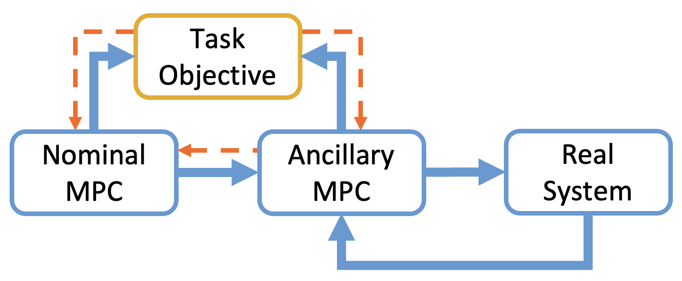
Figure 1: Proposed differentiable robust MPC architecture. Orange dashed arrows show how gradients are passed in our architecture.

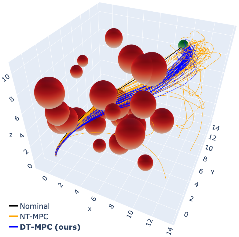
Figure 2: Controlled quadrotor trajectories subject to large disturbances. 50 trajectories are plotted for each algorithm. ‘Nominal’ corresponds to the reference trajectory being tracked by the two algorithms. Our proposed differentiable tube-based MPC (DT-MPC) is safer and more robust than the baseline nonlinear tube-based MPC (NT-MPC).

On the other hand, tube-based approaches have found large success as they are able to leverage the strengths of MPC [27, 34, 13, 50, 30]. These approaches are robust to uncertainty in the dynamics by dividing the online control problem into two optimization layers: a nominal MPC layer and an ancillary MPC layer. The nominal MPC generates a nominal reference trajectory $\bar{\bm{x}}$ in the absence of noise or disturbances. The role of the ancillary MPC is to track the reference trajectory subject to uncertainty in the state of the system. Under certain regularity assumptions, the true state $x$ is guaranteed to lie within some bounded distance from the nominal state $\bar{x}$ — plotting multiple realizations of the state will look like a “tube” centered around the nominal trajectory, from which these approaches derive their name [33, 42]. The use of the ancillary controller makes tube-based approaches more flexible than standard open-loop control through the additional degree of freedom available [34], while the use of MPC keeps these approaches computationally efficient, particularly for real-time applications, e.g., vehicle trajectory planning. While numerous approaches exist that allow the nominal controller of the tube-based MPC to respond to the environment, they are often heuristic in nature or require running an additional optimization, e.g., to select the best candidate starting state for the nominal MPC at every time step [34].

The main contribution of this work is the development of a novel differentiable tube-based MPC (DT-MPC) framework for safe, robust control. Safety is enforced through the use of discrete barrier states [3], which enables scalable constraint satisfaction such that safe planning and control can be executed in real-time. A general differentiable optimal control algorithm is derived that describes how to efficiently pass derivatives through both layers of the MPC architecture (nominal and ancillary controllers). Fig. 1 summarizes the proposed differentiable robust MPC architecture and Fig. 2 demonstrates the proposed DT-MPC algorithm solving a complex quadrotor navigation task in the presence of numerous obstacles. Trajectories controlled under DT-MPC remain safe under large uncertainty and arrive at the goal with higher probability than the baseline.

Additionally, our proposed approach performs gradient updates on the controller parameters in a principled manner and has computational complexity equivalent to that of a single finite-horizon LQR solve. The computation scales linearly with the look-ahead horizon of the MPC, and, therefore, our proposed algorithm is comparable in complexity to conventional MPC. The efficacy of the proposed approach is benchmarked through multiple Monte Carlo simulations on five nonlinear robotics systems, including two systems in the MuJoCo simulator environment [47]. Moreover, timing and gradient error comparisons against state-of-the-art differentiable optimal control methods are provided. Overall, the proposed adaptive, robust MPC algorithm enables robust constraint satisfaction, with the adaptive computation contributing less than 10% of the total runtime.

In summary, the main contributions of this work include:

1. the derivation of a general differentiable optimal control framework enabled through a novel application of the implicit function theorem,

2. the proposition of a differentiable tube-based MPC algorithm that allows the online adaptation of controller parameters to maximize success and safety,

3. extensive benchmarks on five nonlinear robotics systems showing the applicability and generality of the proposed approach.

In Section II, tube-based MPC is reviewed along with embedded discrete barrier states that will be used in the proposed algorithm to enforce safety. Section III presents a generalized differentiable optimal control framework, relating recent advancements in differentiable optimization-based control. In Section IV, a differentiable robust MPC algorithm is presented. Experiments are provided on various robotics systems in Section V. Concluding remarks are given in Section VI.

II Mathematical Background

II-A Tube-based Model Predictive Control

Tube-based MPC approaches design a robust controller for the uncertain, safety-critical system

$$x_{t+1}=f_{\text{true}}(x_{t},u_{t})=f(x_{t},u_{t})+w_{t},$$ (1)

where $t\in\mathbb{N}$ denotes the task time step, $f_{\text{true}}$ describes the true dynamics of the system (e.g., reality), and $f$ is a smooth function which is a model or an approximation of $f_{\text{true}}$ (e.g., physics-based or learned dynamics) that will be used for MPC. $w_{t}\in\mathbb{W}$, where $\mathbb{W}\subseteq\mathbb{R}^{n_{w}}$ is a convex and compact set containing the origin, is a bounded disturbance, which exists due to model uncertainty, random noise, etc. [34]. The system is subject to control constraints $u_{t}\in\mathbb{U}\subset\mathbb{R}^{n_{u}}$, such as physical actuator limits, and safety constraints $x_{t}\in\mathbb{X}\subset\mathbb{R}^{n_{x}}$ that determine the safe operating region of the system of interest. It is assumed that both sets are (strict) superlevel sets of some continuously differentiable functions.

Development of a successful model predictive controller for Eq. 1 relies on the fact that $f$ is a good approximation of the true dynamics $f_{\text{true}}$. However, in practice, the system under study is subject to large dynamical uncertainty through effects such as unmodeled physics, random noise, etc., that results in some error between $f_{\text{true}}$ and $f$, which is captured by the additive disturbance $w$ in the formulation above. The objective will be to bound the deviation of the true state trajectory $\bm{x}\vcentcolon=(x_{0},x_{1},\ldots)$, subject to disturbances, from a reference trajectory $\bar{\bm{x}}\vcentcolon=(\bar{x}_{0},\bar{x}_{1},\ldots)$ that is determined online by solving the nominal MPC problem defined below. Throughout this work, we will use bold letters, such as $\bm{x}$, to represent trajectories of variables. For notational compactness, we define the state-control trajectory as $\bm{\tau}\vcentcolon=(\bm{x},\bm{u})=(x_{0},u_{0},x_{1},u_{1},\ldots,x_{N})$, with planning horizon $N\in\mathbb{N}$. The nominal MPC problem is, therefore, given as:

Problem 1 (Nominal MPC).

$$\bar{\bm{\tau}}= \operatorname*{arg\,min}_{\bm{\tau}}\bar{J}(\bm{\tau})\vcentcolon=\sum_{k=0}^{N-1}\bar{\ell}(x_{k},u_{k})+\bar{\phi}(x_{N}),$$

subject to $$x_{k+1}=f(x_{k},u_{k}),\quad x_{0}=\bar{x}_{t},$$

$$u_{k}\in\mathbb{U},\quad x_{k}\in\bar{\mathbb{X}}\subset\mathbb{X},$$

where $\bar{x}_{t}$ denotes the nominal state at MPC time step $t$ since the controller is employed in a receding horizon fashion and re-optimized at every successor state and $k$ is used to denote predictive quantities. The set $\bar{\mathbb{X}}$ represents a “tightened” constraint set that ensures the true state can be kept safe in the presence of uncertainty [34, 42]. In other words, the nominal state must be kept sufficiently far from the boundary of the true constraint set $\mathbb{X}$, such that the true state of the system will not violate the safety constraints when subject to disturbances.

The nominal controller is often employed in isolation for the control of Eq. 1 by solving 1 online from every true state $x_{t}$. This approach is inherently robust to small uncertainty providing one explanation for the success of nominal MPC in practice, even when 1 is not solved fully at every time step due to restrictions on the available computational resources [37, 1]. However, this approach is only valid when the error between $f_{\text{true}}$ and $f$ is small, i.e., when the disturbances are small. A potential failure mode of nominal MPC when applied for the control of the true system is safety violations caused by this large predictive error [34].

To address this shortcoming, tube-based MPC augments the nominal controller with a feedback model predictive controller that drives the state of the true system towards the nominal trajectory. This controller is known as the ancillary MPC, and solves online at every true state $x_{t}$ the following optimization:

Problem 2 (Ancillary MPC).

$$\begin{aligned} \bm{\tau}^{*}=\operatorname*{arg\,min}_{\bm{\tau}}J(\bm{\tau},t)\vcentcolon={}&\sum_{k=0}^{N-1}\ell(x_{k}-\bar{x}_{k},u_{k}-\bar{u_{k}})\\ &\quad+\phi(x_{N}-\bar{x}_{N}),\end{aligned}$$

$$\text{subject to}\ \ x_{k+1}=f(x_{k},u_{k}),\quad x_{0}=x_{t},$$

$$u_{k}\in\mathbb{U},\quad x_{k}\in\mathbb{X}.$$

Due to the disturbances entering the system Eq. 1, the true state $x_{t}\neq\bar{x}_{t}$ in general. The role of 2 is to drive the true state of the system towards the reference trajectory $\bar{\bm{\tau}}$, under the nominal predictive model $f$. The disturbances affect the optimization through perturbations on the initial state of 2. For more details on the tube-based MPC approach and its analyses, the reader is referred to the works of Mayne et al. [34] and Rawlings et al. [42].

II-B Embedded Barrier States

Consider the safe set $\mathbb{X}$ that is defined as the strict superlevel set of a continuously differentiable function $h:\mathbb{R}^{n_{x}}\to\mathbb{R}$ such that

$$\mathbb{X}\vcentcolon=\{x\in\mathbb{R}^{n_{x}}\ |\ h(x)>0\}.$$

The goal is to render the safe set $\mathbb{X}$ forward invariant, i.e., once the system is in the set, it stays in it for all future times of operation. This is accomplished by defining an appropriate barrier function $B:\mathbb{X}\to\mathbb{R}$ over the safety condition $h$ whose value “blows up” as the state of the system approaches the unsafe region. The idea of embedded barrier states is to augment the system with the state of the barrier and define a new control problem that, when solved, guarantees safety along with other performance objectives [3, 2]. The discrete barrier state (DBaS), denoted $b_{k}$, is defined by the dynamics

$$b_{k+1}=g(x_{k},u_{k},b_{k})=B(h(f(x_{k},u_{k}))-\gamma(B(h(x_{k}))-b_{k}),$$

where $\gamma\in[-1,1]$. Examples of suitable barrier functions include the inverse barrier $B(\zeta)=1/\zeta$ and the log barrier $B(\zeta)=-\log\zeta$. The state of the system to be controlled is then augmented by the barrier state $\hat{x}_{k}=(x_{k},b_{k})$, resulting in the augmented dynamics

$$\hat{x}_{k+1}=\hat{f}(\hat{x}_{k},u_{k})=\begin{bmatrix}f(x_{k},u_{k})\\ g(x_{k},u_{k},b_{k})\end{bmatrix}.$$ (2)

The system Eq. 2 is called the safety-embedded system. The set $\mathbb{X}$ is, therefore, rendered forward invariant if and only if the barrier state of the system remains bounded for all time, given that the system starts in the safe set  [3]. Using the iterative linear-quadratic regulator (iLQR) [26] with embedded DBaS guarantees positive definiteness of the Hessian of the quadratically expanded value function providing guarantees of improvement of safe solutions and convergence (see Theorems 2 and 3 of [3]). The algorithm enjoys a computational efficiency and fast convergence as shown by Almubarak et al. [3] and in the MPC formulation by Cho et al. [14] compared to other safe DDP-based approaches, such as penalty methods, control barrier functions, and augmented Lagrangian methods which require multiple optimization loops and thus do not scale well for real-time applications.

Nonetheless, in the interest of the proposed work and in light of the requirement of starting in the safe region, the solution to the open-loop optimal control problem may be infeasible. A well established solution for barrier-based methods is the relaxed barrier function, which was presented in the linear MPC formulation by Feller and Ebenbauer [19] using the logarithmic barrier function. In dependence of the underlying relaxation, convergence guarantees and and constraint satisfaction were provided. Hence, in this work, recursive feasibility of the tube-based MPC is pledged through the use of a relaxed embedded barrier state that is similar conceptually to the idea of relaxed barrier functions [19]. In essence, the barrier function $B$ is replaced with the relaxed barrier function by taking a Taylor series approximation of the safety function $h$ around a point $\alpha$ close to the constraint “unsatisfaction”, i.e., close to $h=0$, while reserving the advantages of using barrier states within the iLQR. For example, for the inverse barrier function, which is used throughout this work, we take a quadratic approximation and define the strictly monotone and continuously differentiable relaxed barrier function:

$$B_{\alpha}(\zeta)=\begin{cases}1/\zeta&\text{ if }\zeta\geq\alpha,\\ 1/\alpha-(\zeta-\alpha)/\alpha^{2}+(\zeta-\alpha)^{2}/\alpha^{3}&\text{ if }\zeta<\alpha.\end{cases}$$

It is worth noting that the relaxation hyperparameter $\alpha$ determines the amount of relaxation such that $\lim_{\alpha\to 0}B_{\alpha}(\zeta)\to B(\zeta)$. Enabled through differentiable optimization, the framework described in Section IV allows an adaptation scheme to be derived that modulates the amount of relaxation online through updating $\alpha$ based on task performance and feasibility. From the safe MPC via barrier methods perspective, the proposed work provides a novel expansion of the works [3], [14] and [19] to a tube-based MPC algorithm in which the barrier state’s parameters, e.g., dynamics and cost penalization, can be adapted or auto-tuned which greatly improves the controls performance, as we show and discuss in more detail in our experimentation provided in Section V.

In the sequel, we will use $x$ and $f$ to represent the embedded state and the safety-embedded dynamics in our development of the main proposition for notational simplicity. It should be understood that we are working with the safety-embedded system and safety is guaranteed by the boundedness of the barrier state.

III Generalized Differentiable Optimal Control through the Implicit Function Theorem

We derive a general differentiable optimal control framework for computing gradients through the solution of a parameterized optimal control problem ($\bm{\tau}^{*}$ of 3 below). This enables a principled manner through which the parameters of the control problem can be automatically adapted to maximize both safety as well as the desired task performance. The key result here is that the differentiable optimal control algorithm has the same computational complexity as a single finite-horizon LQR solve, namely $O(N)$ in time. This connection with LQR control justifies the use of a Gauss-Newton approximation when backpropagating the derivatives through time, allowing the dynamics and cost derivatives to be reused between the optimal control solver (e.g., iLQR) and the differentiable optimization. Furthermore, we show how the gradient can be accumulated across the trajectory at an $O(1)$ memory cost, independent of the time horizon. This prevents needing to store the entire trajectory of derivatives in memory at once, which is an important consideration for highly parameterized problems, e.g., when neural networks are used to model the dynamics or cost function.

III-A Differentiable Optimization

Our work is inspired by recent developments in implicit differentiation — also known as differentiable optimization — which is an emerging trend in machine learning [4, 6, 11, 10] that studies how to embed optimization processes as end-to-end trainable components into learning-based architectures. Differentiable optimization has seen large success in a wealth of fields such as hyperparameter tuning [8, 28], meta-learning [20, 41], and model-based reinforcement learning and control [5, 24, 17, 22]. This subsection gives a brief overview of differentiable optimization in the context of general optimization problems. These results will be used afterwards to develop a general differentiable optimal control methodology and a differentiable robust MPC framework.

Consider the unconstrained minimization problem

$$z^{*}(\theta)=\operatorname*{arg\,min}_{z}\varphi(z,\theta),$$ (3)

where $\varphi:\mathbb{R}^{n_{z}}\times\mathbb{R}^{n_{\theta}}\to\mathbb{R}$ is smooth, $z$ is the optimization variable, and $\theta$ is a vector of parameters that influence the objective function to be minimized. The implicit function theorem (IFT) provides a precise relation between the optimal solution and the learning parameters by defining $z^{*}$ as an implicit function of $\theta$. Furthermore, it gives an expression for the derivative $\pdv{z^{*}}{\theta}$ — the derivative of the solution with respect to the parameters — and the conditions under which this derivative is defined. This development is necessary when the minimization process Eq. 3 is embedded as a component within, e.g., a deep learning architecture. This allows the parameters of the optimization process to be optimized in an end-to-end fashion through the use of backpropagation and other gradient-based algorithms.

Theorem 1 (Implicit function theorem [25]).

Let $F:\mathbb{R}^{n_{z}}\times\mathbb{R}^{n_{\theta}}\to\mathbb{R}^{n_{z}}$ be a continuously differentiable function. Fix a point $(z_{0},\theta_{0})$ such that $F(z_{0},\theta_{0})=0$. If the Jacobian matrix of partial derivatives $\pdv{F}{z}(z_{0},\theta_{0})$ is invertible, then there exists a function $z^{*}(\cdot)$ defined in a neighborhood of $\theta_{0}$ such that $z^{*}(\theta_{0})=z_{0}$ and

$$\pdv{}{\theta}z^{*}(\theta)=-\left(\pdv{}{z}F(z^{*}(\theta),\theta)\right)^{-1}\pdv{}{\theta}F(z^{*}(\theta),\theta).$$

Proof.

See Krantz and Parks [25] or de Oliveira [15]. ∎

Remark 1.

The condition $F(z_{0},\theta_{0})=0$ may seem restrictive, but the power of Theorem 1 is revealed when we examine the first-order optimality conditions for the minimization problem Eq. 3 — a solution $z^{*}$ to Eq. 3 must satisfy $\nabla_{z}\varphi(z^{*},\theta)=0$. Therefore, the gradient of the function $\varphi$ satisfies the conditions of Theorem 1 as long as the matrix of second-order partial derivatives of $\varphi$ with respect to $z$, namely the Hessian $\varphi_{zz}\vcentcolon=\pdv{}{z}\nabla_{z}\varphi$ is invertible. Furthermore, this generalizes naturally to constrained optimization problems (e.g., $z\in\mathcal{C}\subset\mathbb{R}^{n_{z}}$, for some constraint set $\mathcal{C}$) by considering the appropriate first-order optimality conditions of the problem (e.g., the Karush-Kuhn-Tucker (KKT) conditions). Further discussion can be found in recent works such as [10].

The IFT will be applied in the following subsection to derive a general differentiable optimal control (DOC) framework. This framework will be used to develop a robust MPC algorithm in Section IV that is made adaptive through online differentiable optimization.

III-B General Learning Framework as Bilevel Optimization

We start by motivating the learning problem through the lens of optimal control. For clarity of presentation, we focus on the unconstrained case and provide discussion on the control-constrained case in Appendix G. We consider the following general parameterized optimal control problem of the form

Problem 3 (Parameterized OC).

$$\bm{\tau}^{*}(\theta)=\operatorname*{arg\,min}_{\bm{\tau}}{} J(\bm{\tau},\theta)\vcentcolon=\sum_{k=0}^{N-1}\ell(x_{k},u_{k},\theta)+\phi(x_{N},\theta),$$

subject to $$x_{k+1}=f(x_{k},u_{k},\theta),\quad x_{0}=\xi(\theta),$$

where $\xi$ is a differentiable function denoting the initial condition of the problem (e.g., $\bar{x}_{t}$ for the nominal MPC and $x_{t}$ for the ancillary MPC).

The solution $\bm{\tau}^{*}$ depends on the problem parameters $\theta$, which represent the parts of the dynamics and the objective that are learnable or adaptable, such as cost function weights or unknown constants of a parametric, physics-based model. In practice, these parameters $\theta$ are hand-tuned by a domain expert and fixed during task execution. However, we propose an alternative methodology enabled through differentiable optimization that allows the parameters to be learned and adapted online through minimization of an appropriately specified loss function describing the desired task behavior. The learning objective is therefore defined as the following bilevel optimization over the parameters of 3:

Problem 4 (Learning Problem).

$$\min_{\theta}L(\bm{\tau}^{*}(\theta)),$$ (4)

where $L$ is a differentiable loss function, such as the imitation loss $L=\left\lVert\bm{\tau}^{*}(\theta)-\bm{\tau}_{\text{expert}}\right\rVert^{2}$ where $\bm{\tau}_{\text{expert}}$ is generated by a task expert, e.g., through human demonstration. Without loss of generality, we will assume $L$ does not depend on $\theta$ directly, but the following results can be easily extended to such cases.

The goal will be to establish an efficient methodology to learn the optimal parameters $\theta^{*}$ by solving 4. A natural choice to learn these parameters is through gradient descent. Using the chain rule, the gradient of the objective Eq. 4 with respect to $\theta$ is given as

$$\nabla_{\theta}L(\bm{\tau}^{*}(\theta))=\left(\pdv{\bm{\tau}^{*}(\theta)}{\theta}\right)^{\top}\nabla_{\bm{\tau}}L(\bm{\tau}^{*}(\theta)).$$

The term $\nabla_{\bm{\tau}}L$ can be calculated straightforwardly as it is often a simple analytic expression, e.g., for the imitation learning loss defined earlier, the gradient is given simply as $\nabla_{\bm{\tau}}L=2(\bm{\tau}-\bm{\tau}_{\text{expert}})$. The difficulty arises in calculating the Jacobian $\pdv{\bm{\tau}^{*}}{\theta}$ efficiently — it is not obvious at first how to take derivatives of a solution to 3.

A naïve approach to computing this Jacobian would be to “unroll” the optimization algorithm itself, in a process similar to automatic differentiation (AD). Indeed, this approach is used to great effect in recent work [36, 9]. However, the computational efficiency scales linearly with the number of iterations $K$ necessary to solve 3, making it expensive for highly nonlinear, non-convex problems that might require many iterations to find a good solution. This motivates the use of implicit differentiation and the IFT as introduced in Section III-A, which enables us to derive an analytic expression for the Jacobian $\pdv{\bm{\tau}^{*}}{\theta}$ without requiring full unrolling of the lower-level optimizer.

We begin by introducing the optimality conditions for 3:

Proposition 2 (Optimality conditions of 3).

Define the real-valued function $\mathcal{L}$ for 3, called the Lagrangian, as

$$\begin{aligned} \mathcal{L}(\bm{z},\theta)={}&\sum_{k=0}^{N-1}\ell(x_{k},u_{k},\theta)+\lambda_{k+1}^{\top}(f(x_{k},u_{k},\theta)-x_{k+1})\\ &+\lambda_{0}^{\top}(\xi(\theta)-x_{0})+\phi(x_{N},\theta),\end{aligned}$$

where $\lambda_{k}\in\mathbb{R}^{n_{x}}$, $k=0,1,\ldots,N$ are the Lagrange multipliers for the dynamics and initial condition constraints, and $\bm{z}\vcentcolon=(\bm{\tau},\bm{\lambda})=(\lambda_{0},x_{0},u_{0},\ldots,\lambda_{N},x_{N})$ for notational compactness.

Let $\bm{\tau}^{*}$ be a solution to 3 for fixed parameters $\theta$. Then, there exists Lagrange multipliers $\bm{\lambda}^{*}$ which together with $\bm{\tau}^{*}$ satisfy $\nabla_{\bm{z}}\mathcal{L}(\bm{z}^{*},\theta)=0$.

Proof.

The conditions $\nabla_{\bm{z}}\mathcal{L}(\bm{z}^{*},\theta)=0$ are the KKT conditions for 3. See Appendix A. ∎

For reasons that will be clear soon, it is advantageous to use differential dynamic programming (DDP) [31, 23] as the optimization algorithm to solve 3. DDP uses the principle of dynamic programming [7] to solve 3 efficiently by reparameterizing the minimization over all possible control trajectories as a sequence of minimizations proceeding backwards-in-time.

More formally, DDP iteratively solves for and applies the Newton step $\odif{\bm{z}}$ until convergence:

$$\mathcal{L}_{\bm{z}\bm{z}}\odif{\bm{z}}=-\nabla_{\bm{z}}\mathcal{L},$$ (5)

which requires inverting the Hessian $\mathcal{L}_{\bm{z}\bm{z}}$. However, naïvely inverting this matrix is prohibitively expensive, since the size of the matrix is quadratic in the time horizon of the problem, i.e., the matrix inversion of $\mathcal{L}_{\bm{z}\bm{z}}$ is $O(N^{3})$. To remedy this, we utilize dynamic programming and the sparsity induced by the constraints of the control problem to rewrite Eq. 5 as a series of backwards difference equations — in optimal control, these are known as the Riccati equations. This allows the solution of Eq. 5 to be computed with efficiency linear in the horizon $N$. This same insight will be key to efficiently computing the implicit derivative of 3 defined below.

Proposition 3 (Implicit derivative of 3).

Let $\bm{\tau}^{*}$ be a solution to 3 for fixed parameters $\theta$. By Proposition 2, Theorem 1 holds with $F=\nabla_{\bm{z}}\mathcal{L}$. Furthermore, the Jacobian $\pdv{\bm{z}^{*}}{\theta}$ is given as

$$\pdv{}{\theta}\bm{z}^{*}(\theta)=-\mathcal{L}_{\bm{z}\bm{z}}^{-1}\mathcal{L}_{\bm{z}\theta}.$$ (6)

Proof.

See Appendix B. ∎

Remark 2.

Note that the structure of both Eq. 5 and Eq. 6 here is similar, with the only difference being the fact that the inverse Hessian is applied to the gradient $\nabla_{\bm{z}}\mathcal{L}$ in Eq. 5 while it is multiplied with a matrix of partial derivatives $\mathcal{L}_{\bm{z}\theta}$ in Eq. 6. In fact, solving Eq. 6 directly allows one to derive the Pontryagin differentiable programming (PDP) framework proposed by Jin et al. [24], which was originally derived by directly differentiating the KKT conditions of 3 with respect to $\theta$.

Corollary 4 (Pontryagin differentiable programming [24]).

Let the conditions of Proposition 2 and Proposition 3 hold. Then, the differentiable Pontryagin conditions ((Eq. (13) of Jin et al. [24]) are equivalent to solving the linear system Eq. 6.

Proof.

This can be seen by expanding the matrix multiplication in Eq. 6. See Appendix C. ∎

Corollary 4 implies that rather than differentiating the Pontryagin conditions directly, a more general framework can be derived by applying the IFT to the control problem. Furthermore, the IFT describes the conditions under which this derivative exists and can be calculated, which generalizes the work by Jin et al. [24].

However, this process requires solving the set of matrix equations in Eq. 6, i.e., a matrix control system backwards-in-time. This is inefficient due to requiring the computation and storage of the intermediate Jacobians $\pdv{x_{k}^{*}}{\theta}$ and $\pdv{u_{k}^{*}}{\theta}$ along the entire trajectory. We will show next that an improvement can be made by taking advantage of an insight similar to the computation of vector-Jacobian products in AD.

Theorem 5 (Differentiable Optimal Control).

Let $\bm{z}$ denote the augmented vector consisting of $\bm{\tau}$ and $\bm{\lambda}$. In addition, let the conditions of Proposition 2 and Proposition 3 hold. Then, the gradient of the loss $L$ with respect to $\theta$ is given by

$$\nabla_{\theta}L(\bm{z}^{*}(\theta))=\mathcal{L}_{\theta\bm{z}}\delta\bm{z},$$ (7)

where the vector $\delta\bm{z}$ is given by solving the linear system

$$\mathcal{L}_{\bm{z}\bm{z}}\delta\bm{z}=-\nabla_{\bm{z}}L.$$ (8)

Proof.

See Appendix D. ∎

Remark 3.

Theorem 5 shows that, rather than calculating $\mathcal{L}_{\bm{z}\bm{z}}^{-1}\mathcal{L}_{\bm{z}\theta}$ directly as in Eq. 6, we can instead start by solving the linear system Eq. 8 for the vector $\delta\bm{z}$. Then, the gradient $\nabla_{\theta}L$ can be computed through a simple matrix multiplication (Eq. 7). This general algorithm is presented in Algorithm 1, whose full derivation is provided in the Appendix E.

Input: Derivatives of $\mathcal{L}$ (equivalently $f$, $\ell$, $\phi$, and $\xi$) and $L$ along the solution $\bm{z}^{*}$

Output: Gradient of upper-level loss $\nabla_{\theta}L$

1

2$\widetilde{\bm{V}}_{x},\bm{V}_{xx},\widetilde{\bm{k}},\bm{K}\leftarrow$ Solve backward pass equations (Algorithm 3 of Appendix E);

$\nabla_{\theta}L\leftarrow$ Solve forward pass equations (Algorithm 4 of Appendix E);

Algorithm 1 Differentiable Optimal Control (DOC)

As established earlier and presented in Algorithm 1, solving systems of the form Eq. 8 can be accomplished through the DDP equations by replacing the gradient of the Lagrangian $\nabla_{\bm{z}}\mathcal{L}$ in Eq. 5 with the gradient of the upper-level loss $\nabla_{\bm{z}}L$. This fact illustrates the connection between the lower-level control problem (3) and the upper-level learning problem (4) and highlights the advantages of implicit differentiation — by taking advantage of the structure of the lower-level problem, an efficient algorithm can be derived for computing the derivatives of the upper-level problem. This algorithm is presented in Algorithm 1 and has $O(N)$ time complexity and $O(1)$ memory complexity, where $N$ is the look-ahead horizon of the MPC. Therefore, our approach scales similarly to conventional MPC, and furthermore, this connection shows that it is advantageous to use DDP as the lower-level control solver since the necessary derivatives for DDP (e.g., $\mathcal{L}_{\bm{z}\bm{z}}$) can be reused during the computation of the parameter gradient in Eqs. 7 and 8.

Additionally, by deriving Theorem 5 through the IFT, the proposed DOC methodology is independent of how a solution to 3 is generated. In other words, rather than begin from an existing optimal control algorithm, as is presented by, e.g., Amos et al. [5] in the context of iLQR or Dinev et al. [17] in the context of DDP, we show that a single framework generalizes to any control algorithm, as long as the solution itself satisfies the conditions of Proposition 2.

An additional benefit of the independence from the optimal control solver is the fact that the gradient computation does not depend on the number of solver iterations $K$ required to reach a solution. While unrolling a numerical solver through AD would incur computational complexity $O(KN)$ in both time and memory, our approach maintains $O(N)$ complexity independent of the underlying solver. These facts allow the gradient computation to be efficient enough for the adaptation of a real-time MPC controller. Further speedups can be incorporated by adopting a Gauss-Newton approximation when solving Eq. 8, at the cost of numerical error. The particular choice of a Gauss-Newton approximation allows one to derive the seminal differentiable MPC by Amos et al. [5]. This is formalized in the following corollary:

Corollary 6 (Differentiable MPC [5]).

Differentiable MPC as proposed by Amos et al. [5] is equivalent to using a Gauss-Newton approximation when solving Eq. 8.

Proof.

See Appendix F. ∎

Timing and gradient error comparisons between our proposed Algorithm 1 and the algorithms of Amos et al. [5], Jin et al. [24], and Dinev et al. [17] are provided in Appendix H.

IV Differentiable Tube-based MPC

When experiencing large disturbances, MPC under the nominal system model can fail. Although tube-based MPC is designed to tackle such a problem, determining the cost parameters necessary to achieve robustness is difficult in practice due to the nonlinear dependence between the nominal controller and the ancillary controller. Moreover, tuning fixed parameters offline to work for one scenario does not generalize for online, real-time MPC applications, where there may exist, e.g., a large sim-to-real gap. This motivates a method that can update the robust controller parameters automatically and online.

Under the differentiable optimal control framework presented in Section III, the nominal controller seeks to optimize the parameterized safe nominal trajectory $\bar{\bm{\tau}}$ in the absence of disturbances by solving the following optimization:

Problem 5 (Differentiable Nominal MPC).

$$\begin{aligned} \bm{\bar{\tau}}(\bar{\theta})=\operatorname*{arg\,min}_{\bm{\tau}}\bar{J}(\bm{\tau},\bar{\theta})\vcentcolon={}&\sum_{k=0}^{N-1}\bar{\ell}(x_{k},u_{k},\bar{\theta})+\bar{\phi}(x_{N},\bar{\theta}),\end{aligned}$$

$$\begin{aligned} \text{subject to}\ \ &x_{k+1}=f(x_{k},u_{k},\bar{\theta}),\quad x_{0}=\bar{x}_{t},\\ &u_{k}\in\mathbb{U},\quad x_{k}\in\bar{\mathbb{X}}(\bar{\theta})\subset\mathbb{X}.\end{aligned}$$

Here “bar” denotes nominal quantities and $\bar{\mathbb{X}}$ represents the tightened state constraint set (see 1 of Section II-A), now parameterized by $\bar{\theta}$. This parameterization enables the online determination of effective size of $\bar{\mathbb{X}}$ through differentiable optimization, instead of hand tuning it using, e.g., offline data.

In our algorithm, the parameterization of $\bar{\mathbb{X}}$ with $\bar{\theta}$ is enabled through the adoption of barrier states for enforcing safety constraints and their penalizations in the cost function. In the use of DBaS as described in Section II-B, an additional state within the cost function is introduced. For example, for the cost function $J$, we will assume that it has the partitioned form $\hat{J}=J+\sum_{k=0}^{N}q_{b}b_{k}^{2}$, with $q_{b}>0$ being a tunable parameter quantifying the strength of the barrier. This enables the online determination of the effective size of the feasible region $\bar{\mathbb{X}}$ through adaptation of $q_{b}$ based on task performance and predicted safety of the true system. Nonetheless, it should be noted that the proposed method is general and this is one specific choice that the authors find to work very well in practice. We will show different controller designs and solutions in Section V.

Consequently, the differentiable ancillary MPC problem is given as follows:

Problem 6 (Differentiable Ancillary MPC).

$$\begin{aligned} \bm{\tau}^{*}(\theta)=\operatorname*{arg\,min}_{\bm{\tau}}J(\bm{\tau},\theta,t)\vcentcolon=&\sum_{k=0}^{N-1}\ell(x_{k}-\bar{x}_{k},u_{k}-\bar{u_{k}},\theta)\\ &\quad+\phi(x_{N}-\bar{x}_{N},\theta),\end{aligned}$$

$$\text{subject to}\ \ x_{k+1}=f(x_{k},u_{k},\theta),\quad x_{0}=x_{t},\quad u_{k}\in\mathbb{U}.$$

It is worth highlighting again that the safety constraint does not appear in 6 as the state equation represents the safety-embedded system through the use of the DBaS as mentioned earlier. This has the effect of increasing the state dimension of the problem but does not affect the algorithm computationally as the input dimension is unchanged (DDP-based methods scale with the size of the control input but not the state input [31]). Note that this means that $\theta$ includes the DBaS tunable parameters such as $\gamma$ and $\alpha$ for the DBaS feedback and the relaxation of the barrier condition for the recursive feasibility of the algorithm when needed.

Through the introduction of the DBaS, an additional degree of freedom that helps determine the tightness of the constraint satisfaction is added to the control problem. Therefore, our method is able to adjust the conservativeness of the nominal controller while also adapting the tube shape and size by updating the cost parameters of the ancillary controller based on the disturbances encountered. This allows for an efficient computational and engineering framework for robust control. Namely, the nominal controller can be tuned for task completion in the well-understood deterministic case, as is typical in standard nonlinear control design. The adaptive ancillary controller can then be used to augment the nominal controller for robustness, responding to disturbances when necessary.

Next, we propose an algorithm that applies the DOC methodology presented in Section III to the real-time tuning of tube-based controllers of the form given by 5 and 6. In order to optimize both the nominal and ancillary controller, we propose to use a loss function of the form

$$L(\bm{\tau}^{*}(\theta),\bar{\bm{\tau}}(\bar{\theta}))=\left\lVert\bm{x}^{*}(\theta)-\bar{\bm{x}}(\bar{\theta})\right\rVert_{2}^{2}+\left\lVert\bm{b}^{*}(\theta)\right\rVert_{2}^{2},$$ (9)

but modify the loss in the experiments as necessary to capture task-specific objectives. Notably, this choice of objective is beneficial as it captures the primary goal of tube-based MPC, which is to drive the true state $x$ towards the nominal state $\bar{x}$ while maintaining safety of the true system. Furthermore, this choice allows the parameters of the nominal MPC to be updated based on the expected performance of the ancillary MPC, allowing the nominal MPC to respond to the environment in an optimal manner. The general differentiable tube-based MPC algorithm is presented in Algorithm 2 and is a straightforward application of Algorithm 1.

Input: Initial nominal parameters $\bar{\theta}$ and ancillary parameters $\theta$, learning rate $\eta$, task horizon $H$

1

2$\bar{x}_{0}\leftarrow x_{0}$;

3for $t=0,\ldots,H$ do

4      

5      $\bar{\bm{\tau}}(\bar{\theta})\leftarrow$ Solve 5 starting from $\bar{x}_{t}$;

6      $\bm{\tau}^{*}(\theta)\leftarrow$ Solve 6 starting from $x_{t}$;

7      $\nabla_{\bar{\theta}}L,\nabla_{\theta}L\leftarrow$ Compute gradients of $L(\bm{\tau}^{*}(\theta),\bar{\bm{\tau}}(\bar{\theta}))$ using Algorithm 1;

      // Gradient descent step

8       $\bar{\theta}\leftarrow\bar{\theta}-\eta\nabla_{\bar{\theta}}L$;  $\theta\leftarrow\theta-\eta\nabla_{\theta}L$;  

      // True and nominal dynamics

9       $x_{t+1}\leftarrow f(x_{t},u_{t}^{*})+w_{t}$;  $\bar{x}_{t+1}\leftarrow f(\bar{x}_{t},\bar{u}_{t})$;

10 end for

Algorithm 2 Differentiable Tube-based Model Predictive Control (DT-MPC)

Figure 1 visualizes the information and gradient flow of the proposed architecture. In summary, Algorithm 2 solves the nominal MPC 5 from the current nominal state $\bar{x}_{t}$ with $\bar{\theta}$ fixed and consisting of the DBaS parameters and task-dependent cost function parameters. The solution $\bar{\bm{\tau}}$ is passed to the ancillary MPC 6 which is solved starting from the current state $x_{t}$ for fixed $\theta$ that consists of the DBaS parameters and the cost function parameters that determine the tracking cost of the feedback controller. Gradients of a task-dependent loss function are computed with respect to both the nominal and the ancillary parameters through Algorithm 1, and a gradient update is performed (Line 6). Finally, the ancillary control is sent to the true system, and the controller receives an observation of the next state perturbed by the disturbance $w_{t}$. Meanwhile, the nominal system propagates forward in the absence of noise or uncertainty, and the process is repeated.

The proposed algorithm improves upon and solves problems within previous contributions in multiple directions. In one aspect, it can be clearly seen that for such a problem, many parameters need to be tuned and carefully selected, e.g., through trial and error, while the proposed algorithm provides a theoretically sound and practical approach to auto-tune the different parameters involved to achieve a high level of autonomy. Indeed, not only does the proposed algorithm provide robustness to the safe trajectory optimization problem through tube-based MPC, but it also provides adaptability and auto-tuning of the DBaS weight in the DBaS-iLQR MPC formulation by Cho et al. [14]. Rather than keeping the weight fixed, which might result in an overly-conservative solution that withstands disturbances but prevents task completion, the proposed DT-MPC results in an adaptive, time-varying weight that is used to solve the safety-critical optimal control problem and therefore better approximates the original optimal control problem. This is especially true when the nominal controller uses a poor model that might guide the ancillary controller to violate the safety condition. Moreover, through the use of relaxed barriers along with DDP, the work by Feller and Ebenbauer [19] is generalized to the nonlinear case while auto-tuning the relaxation parameter $\alpha$ online. This allows us to recover the original barrier when needed.

V Experiments

The generality of the proposed DT-MPC is established through benchmarks on five nonlinear robotics systems subject to highly non-convex constraints such as dense obstacle fields. In the experiments that follow, the nominal MPC is tuned to perform the task successfully and then the algorithms are deployed on the true system, without further tuning. This puts the proposed framework to the test, especially in comparison to the non-adaptive, nonlinear tube-based MPC. This suite of experiments showcases how the differentiable framework enables robust control through online adaptation of the necessary parameters to accomplish the task while maintaining safety. The results are summarized in Table I, which details the overall task completion percentage as well as the percentage of safety violations for each algorithm. Specific numerical information related to the experiments, such as the parameterization for each controller as well as timing comparisons between algorithms, is provided in Appendix I.

	Dubins Vehicle		Quadrotor		Robot Arm		Cheetah		Quadruped
	Successes	Violations	Successes	Violations	Successes	Violations	Successes	Violations	Successes	Violations
NT-MPC	14%	0%	14%	20%	0%	56%	26%	4%	20%	0%
DT-MPC (ours)	100%	0%	76%	4%	78%	10%	70%	0%	64%	0%

TABLE I: Success and safety violation percentage for each algorithm over 50 trials per task. For successes, higher is better, while for violations, lower is better. Success is defined as arriving close to a target state, while a violation is defined as colliding with an obstacle or violating the safety constraints. The magnitude of disturbances are upper-bounded by $0.05$, $0.1$, $0.1$, $0.05$ and $0.05$ for each system, respectively.

V-A Dubins Vehicle

As an illustrative example, a Dubins vehicle task is set up where the goal is to reach a target state of $(10,10)$ $\text{\,}\mathrm{m}$ while avoiding obstacles, as shown in Fig. 3. The vehicle starts at the origin facing the upper-right direction and, at every timestep, receives disturbances sampled uniformly from the range $[-0.05,0.05]$ in both the xy position as well as its orientation. The nominal MPC parameters are kept fixed, while the ancillary MPC is allowed to adapt through minimization of the loss defined in Eq. 9.

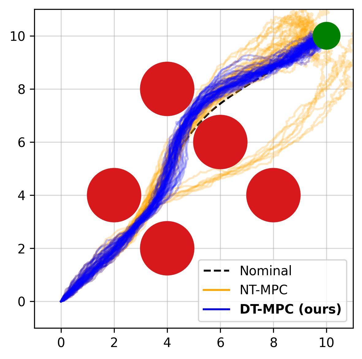
Figure 3: Controlled Dubins vehicle trajectories subject to large noise. NT-MPC trajectories diverge from the nominal trajectory and the uncertainty increases over time. Meanwhile, DT-MPC adapts to the environment, maintaining safety and robust task performance.

Controlled trajectories under both tube-based MPC algorithms for 50 different disturbance realizations are plotted in Fig. 3. DT-MPC bounds the true system within a safer tube around the nominal trajectory, and the trajectories remain on the same side of the central obstacle. Additionally, the size of the tube is updated based on safety (proximity to obstacles), while the NT-MPC tube grows as the trajectory proceeds.

While both algorithms remain safe and avoid collisions (see Table I), only DT-MPC is able to complete the task the majority of the time. This is attributed to the fact that the tube around the nominal trajectory is both tighter and safer allowing for more robust control. Furthermore, a qualitatively beneficial emergent behavior is observed where the tube of trajectories becomes tighter around the nominal trajectory when the state is most unsafe.

V-B Quadrotor

The second experiment is a quadrotor navigating through a dense field of spherical obstacles, where the goal is to reach the target location of $(10,10,10)$ $\text{\,}\mathrm{m}$, starting from the origin, in the presence of large disturbances. The system experiences disturbances in the position and Euler angles sampled uniformly from the range $[-0.01,0.01]$, while disturbances in the linear and angular velocities are sampled from a larger range of $[-0.1,0.1]$ — this choice emulates large unmodeled forces and moments in the dynamics. Like the Dubins vehicle experiment, the nominal MPC parameters are fixed, while the ancillary MPC is adapted through minimization of Eq. 9, balancing tracking performance with safety.

From Fig. 2 and Table I, it can be seen that NT-MPC is unable to maintain robustness, resulting in 20% of the trajectories hitting obstacles or diverging from the nominal system, and only 14% of trajectories are able to solve the task. On the other hand, the proposed DT-MPC bounds the true system within a safer tube around the nominal trajectory by tuning the ancillary MPC in real-time, drastically increasing the success rate to 76% with only 4% violations.

V-C Robot Arm

Figure 4: Environment for the robot arm task.

A 6-DOF torque-controlled robot arm with three links is used to test the ability of the proposed approach to adapt both the nominal and ancillary controller to respond to disturbances. A visualization for the task is given in Fig. 4. The goal is to bring the end effector to the location of $(2,0,1)$ $\text{\,}\mathrm{m}$, starting from a random initial orientation, in the presence of large disturbances and obstacles.

Disturbances in the angles and angular velocities at every timestep are sampled uniformly from the ranges $[-0.01,0.01]$ $\text{\,}\mathrm{rad}$ and $[-0.1,0.1]$ $\text{\,}\mathrm{rad}\text{\,}{\mathrm{s}}^{-1}$, respectively, which, like the quadrotor experiment, corresponds to very large unmodeled forces and moments. For this task, the nominal controller (tuned for deterministic task completion) is too aggressive for the magnitude of disturbances received, leading to a large number of failures even when controlled using NT-MPC. Meanwhile, the proposed DT-MPC is able to adapt the nominal controller to be less aggressive (by tuning the barrier state cost weights) while simultaneously tuning the ancillary controller to be more robust.

V-D Cheetah

(a) Nonlinear tube-based MPC. The lack of adaptation causes the cheetah to flip over.

(b) Differentiable tube-based MPC. Adaptation produces a stable running behavior and allows the cheetah to reach the target safely.

Figure 5: Comparison of tube-based MPC approaches on the DeepMind Control Suite cheetah robotics system [48].

In the next experiment, we design a locomotion task for the cheetah model provided by the DeepMind Control Suite [48]. The objective of the controller is to drive the cheetah to a target position of $5\text{\,}\mathrm{m}$ in $3\text{\,}\mathrm{s}$, requiring an average velocity of $1.67\text{\,}\mathrm{m}\mathrm{/}\mathrm{s}$, while maintaining safe operation. Safety is enforced by constraining the pitch angle of the cheetah to stay within the range $[-\pi/4,\pi/4]$ — when the pitch angle becomes larger than these bounds, it is difficult in general for the cheetah to recover, especially in the presence of large noise. Disturbances are injected into the velocity states and are sampled uniformly from $[-0.05,0.05]$. Additional control noise is added sampled from $\mathcal{N}(0,0.02)$.

For DT-MPC, we use the loss $L=\left\lVert\bm{p}_{x}^{*}-\bar{\bm{p}}_{x}\right\rVert_{2}^{2}+\left\lVert\bm{b}^{*}\right\rVert_{2}^{2}$, where $p_{x}$ is the state corresponding to the x-position, and allow the running cost and barrier state parameters of the nominal MPC and the ancillary MPC to be adapted online. Notably, the terminal cost is kept fixed for the nominal MPC to ensure the task objective information is not lost. The loss function is selected to only penalize the x-position as otherwise all of the states are weighted equally and the ancillary MPC prefers to default to a stable (yet safe) configuration rather than complete the task.

The results in Table I show that, while NT-MPC fails to reach the target in the majority of the cases and occasionally violates the safety of the system, the proposed DT-MPC is able to adapt the entire robust MPC architecture for task completion while maintaining safe control. A sample visualization of one trial per algorithm is provided in Fig. 5.

V-E Quadruped

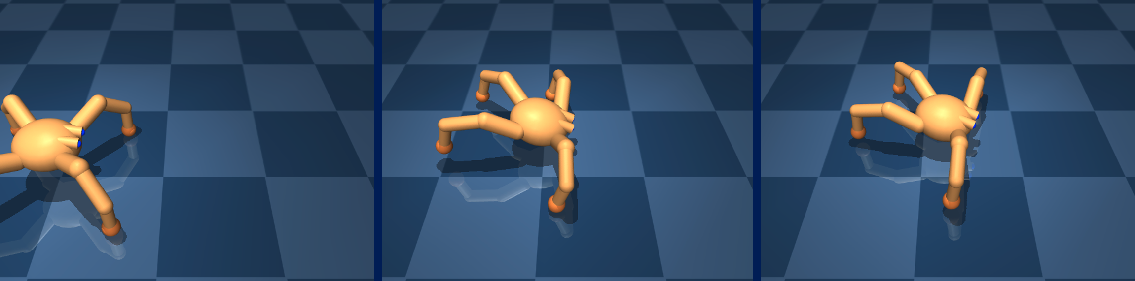
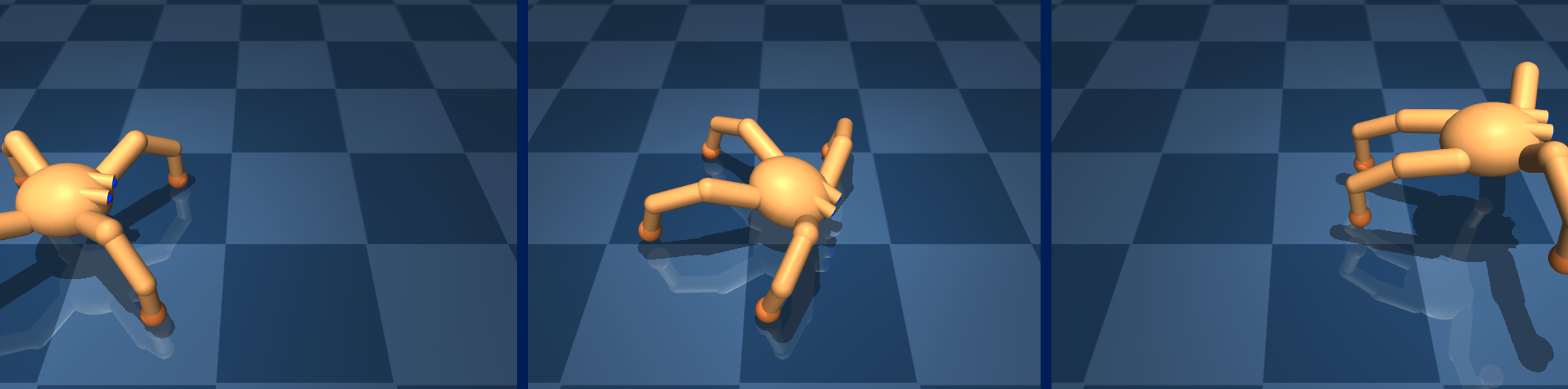
(a) Nonlinear tube-based MPC. The quadruped gets stuck because the true state diverges from the nominal due to the disturbances.

(b) Differentiable tube-based MPC. The adaptation enables the quadruped to successfully reach the target despite large disturbances.

Figure 6: Comparison of tube-based MPC approaches on the DeepMind Control Suite quadruped system [48].

The final experiment is a locomotion task using the quadruped model provided by the DeepMind Control Suite [48]. The system has 56 states and 12 controls, and the objective is to drive the quadruped towards a target position of $2.5\text{\,}\mathrm{m}$ in $2\text{\,}\mathrm{s}$ requiring an average velocity of $1.25\text{\,}\mathrm{m}\mathrm{/}\mathrm{s}$. Dynamical uncertainty is simulated by perturbing the velocity states with a disturbance sampled from the range $[-0.05,0.05]$ and introducing control noise sampled from $\mathcal{N}(0,0.01)$. Safety is determined by constraining the Euler angles of the system such that the quadruped does not flip over ($[-\pi/2,\pi/2]$ for the roll and yaw angles and $[-1.0,1.0]$ for the pitch angle). Figure 6 provides a visualization of the model and task.

The loss for DT-MPC is selected to be the same as the cheetah experiment, namely $L=\left\lVert\bm{p}_{x}^{*}-\bar{\bm{p}}_{x}\right\rVert_{2}^{2}+\left\lVert\bm{b}^{*}\right\rVert_{2}^{2}$. Similarly, both the nominal and ancillary MPC running cost and barrier state parameters are adapted online.

Like the robot arm and cheetah experiment, the nominal controller in NT-MPC has no awareness of the true task performance. Therefore, the system controlled under NT-MPC has difficulty reaching the target. While the deterministic nominal trajectory reaches the target state during every trial, the ancillary controller cannot keep up with the desired aggressive jumping maneuver due to the disturbances. This causes the gap between the nominal trajectory and true state to grow over time. Meanwhile, the system controlled under DT-MPC allows the nominal controller to adapt based on the tracking performance of the ancillary MPC. Furthermore, the ancillary MPC is adapted online to keep the system safe. This results in successful aggressive jumping maneuvers such as the one shown in the bottom right of Fig. 6. Overall, DT-MPC remains safe while increasing the task success rate by over 200% (20% success rate for NT-MPC vs. 64% success rate for DT-MPC).

VI Conclusion

This work has proposed a general algorithm for differentiable optimal control with a unified perspective derived from applying the implicit function theorem to the lower-level control problem. We have detailed how to apply the methodology to the real-time tuning of tube-based MPC controllers, illustrating a principled manner for which to learn the problem parameters of any nonlinear control algorithm. The generality of the method is verified for the robust control of five nonlinear systems in the presence of various safety constraints and large uncertainties. We emphasize the fact that our proposed architecture enables the real-time tuning of any tube-based MPC algorithm. Promising future extensions of the work include learning the dynamical uncertainty and adapting the model used by the MPC controllers.

Appendix A Proof of Proposition 2

Proposition 2 (Optimality conditions of 3).

Define the real-valued function $\mathcal{L}$ for 3, called the Lagrangian, as

$$\begin{aligned} \mathcal{L}(\bm{z},\theta)={}&\sum_{t=0}^{N-1}\ell(x_{k},u_{k},\theta)+\lambda_{k+1}^{\top}(f(x_{k},u_{k},\theta)-x_{k+1})\\ &+\lambda_{0}^{\top}(\xi(\theta)-x_{0})+\phi(x_{N},\theta),\end{aligned}$$ (10)

where $\lambda_{k}\in\mathbb{R}^{n_{x}}$, $k=0,1,\ldots,N$ are the Lagrange multipliers for the dynamics and initial condition constraints, and $\bm{z}\vcentcolon=(\bm{\tau},\bm{\lambda})=(\lambda_{0},x_{0},u_{0},\ldots,\lambda_{N},x_{N})$ for notational compactness.

Let $\bm{\tau}^{*}$ be a solution to 3 for fixed parameters $\theta$. Then, there exists Lagrange multipliers $\bm{\lambda}^{*}$ which together with $\bm{\tau}^{*}$ satisfy $\nabla_{\bm{z}}\mathcal{L}(\bm{z}^{*},\theta)=0$.

Proof.

Taking the gradient of the Lagrangian Eq. 10 with respect to each argument yields the following set of equations:

$$\nabla_{\lambda_{0}}\mathcal{L} =\xi(\theta)-x_{0}^{*},$$

$$\nabla_{\lambda_{k+1}}\mathcal{L} =f(x_{k}^{*},u_{k}^{*},\theta)-x_{k+1}^{*},$$

$$\nabla_{x_{k}}\mathcal{L} =\ell_{x_{k}}+f_{x_{k}}^{\top}\lambda_{k+1}-\lambda_{k},$$

$$\nabla_{u_{k}}\mathcal{L} =\ell_{u_{k}}+f_{u_{k}}^{\top}\lambda_{k+1},$$

$$\nabla_{x_{N}}\mathcal{L} =\phi_{x}-\lambda_{N},$$

where functions are evaluated at the points $x_{k}^{*},u_{k}^{*},\theta$ along the solution $\bm{\tau}^{*}$ and the abbreviated notation $\ell_{x_{k}}$, $f_{u_{k}}$, etc. is used for gradients and partial derivatives. The first two equations are equal to zero because a feasible solution satisfies the initial condition and dynamics constraints of 3. The remaining equations, when set equal to zero, yield a set of backward equations defining the optimal Lagrange multipliers $\bm{\lambda}^{*}$:

$$\lambda_{k}^{*} =\ell_{x_{k}}+f_{x_{k}}^{\top}\lambda_{k+1}^{*},\quad\lambda_{N}^{*}=\phi_{x},$$

$$0 =\ell_{u_{k}}+f_{u_{k}}^{\top}\lambda_{k+1}^{*}.$$

These facts together imply the statement of the proposition. These conditions $\nabla_{\bm{z}}\mathcal{L}(\bm{z}^{*},\theta)=0$ are known as the KKT conditions, and are equivalent to the discrete-time Pontryagin maximum/minimum principle (PMP) (see, e.g., Appendix C of Jin et al. [24]). ∎

Appendix B Proof of Proposition 3

Proposition 3 (Implicit derivative of 3).

Let $\bm{\tau}^{*}$ be a solution to 3 for fixed parameters $\theta$. By Proposition 2, Theorem 1 holds with $F=\nabla_{\bm{z}}\mathcal{L}$. Furthermore, the Jacobian $\pdv{\bm{z}^{*}}{\theta}$ is given as

$$\pdv{}{\theta}\bm{z}^{*}(\theta)=-\mathcal{L}_{\bm{z}\bm{z}}^{-1}\mathcal{L}_{\bm{z}\theta}.$$

Proof.

Let Proposition 2 hold for $\bm{z}^{*}=(\bm{\tau}^{*},\bm{\lambda}^{*})$. Furthermore, assume the Hessian $\mathcal{L}_{\bm{z}\bm{z}}$ evaluated at $\bm{z}^{*}$ is nonsingular, which can be ensured through, e.g., Levenberg–Marquardt regularization [46]. Since $\nabla_{\bm{z}}\mathcal{L}(\bm{z}^{*},\theta)=0$, the gradient $\nabla_{\bm{z}}\mathcal{L}$ satisfies the conditions of Theorem 1, and the statement of the proposition follows naturally. ∎

Appendix C Proof of Corollary 4

Corollary 4 (Pontryagin differentiable programming [24]).

Let the conditions of Proposition 2 and Proposition 3 hold. Then, the differentiable Pontryagin conditions ((Eq. (13) of Jin et al. [24]) are equivalent to solving the linear system Eq. 6.

Proof.

First, let us state the differentiable Pontryagin conditions [24] in the notation of this paper:

$$\pdv{x_{0}}{\theta} =\xi_{\theta},$$ (11)

$$\pdv{x_{k+1}}{\theta} =f_{x_{k}}\pdv{x_{k}}{\theta}+f_{u_{k}}\pdv{u_{k}}{\theta}+f_{\theta_{k}},$$

$$\pdv{\lambda_{k}}{\theta} =\mathcal{L}_{xx}^{(k)}\pdv{x_{k}}{\theta}+\mathcal{L}_{xu}^{(k)}\pdv{u_{k}}{\theta}+f_{x_{k}}^{\top}\pdv{\lambda_{k+1}}{\theta}+\mathcal{L}_{x\theta}^{(k)},$$

$$0 =\mathcal{L}_{ux}^{(k)}\pdv{x_{k}}{\theta}+\mathcal{L}_{uu}^{(k)}\pdv{u_{k}}{\theta}+f_{u_{k}}^{\top}\pdv{\lambda_{k+1}}{\theta}+\mathcal{L}_{u\theta}^{(k)},$$

$$\pdv{\lambda_{N}}{\theta} =\phi_{xx}\pdv{x_{N}}{\theta}+\phi_{x\theta},$$

where all derivatives are evaluated along the solution $\bm{z}^{*}$. The notation $\mathcal{L}_{ux}^{(k)}$ denotes the block of the Hessian of the Lagrangian Eq. 10 corresponding to $u_{k}^{*},x_{k}^{*}$, see below. Let us write explicitly the form of the Jacobian $\pdv{\bm{z}^{*}}{\theta}=(\ldots,\pdv{\lambda_{k}}{\theta},\pdv{x_{k}}{\theta},\pdv{u_{k}}{\theta},\pdv{\lambda_{k+1}}{\theta},\ldots,\pdv{\lambda_{N}}{\theta},\pdv{x_{N}}{\theta})$, the Hessian of the Lagrangian

$$\mathcal{L}_{\bm{z}\bm{z}}=\bNiceMatrix[margin,first-row,last-col]{\color[rgb]{1,0,0}\lambda_{k}}&{\color[rgb]{1,0,0}x_{k}}{\color[rgb]{1,0,0}u_{k}}{\color[rgb]{1,0,0}\lambda_{k+1}}{\color[rgb]{1,0,0}x_{N}}\\ \ddots-I{\color[rgb]{1,0,0}\lambda_{k}}\\ -I\mathcal{L}_{xx}^{(k)}\mathcal{L}_{xu}^{(k)}f_{x_{k}}^{\top}{\color[rgb]{1,0,0}x_{k}}\\ \mathcal{L}_{ux}^{(k)}\mathcal{L}_{uu}^{(k)}f_{u_{k}}^{\top}{\color[rgb]{1,0,0}u_{k}}\\ f_{x_{k}}f_{u_{k}}{\color[rgb]{1,0,0}\lambda_{k+1}}\\ \ddots-I\\ -I\phi_{xx}{\color[rgb]{1,0,0}x_{N}},$$ (12)

and the Hessian $\mathcal{L}_{\bm{z}\theta}=(\xi_{\theta},\ldots\mathcal{L}_{x\theta}^{(k)},\mathcal{L}_{u\theta}^{(k)},f_{\theta_{k}},\ldots,\phi_{x\theta})$. Expanding the matrix multiplication $\mathcal{L}_{\bm{z}\bm{z}}\pdv{\bm{z}^{*}}{\theta}=-\mathcal{L}_{\bm{z}\theta}$ yields

$$\begin{split}-\pdv{x_{0}}{\theta}&=-\xi_{\theta},\\ -\pdv{\lambda_{k}}{\theta}+\mathcal{L}_{xx}^{(k)}\pdv{x_{k}}{\theta}+\mathcal{L}_{xu}^{(k)}\pdv{u_{k}}{\theta}+f_{x_{k}}^{\top}\pdv{\lambda_{k+1}}{\theta}&=-\mathcal{L}_{x\theta}^{(k)},\\ \mathcal{L}_{ux}^{(k)}\pdv{x_{k}}{\theta}+\mathcal{L}_{uu}^{(k)}\pdv{u_{k}}{\theta}+f_{u_{k}}^{\top}\pdv{\lambda_{k+1}}{\theta}&=-\mathcal{L}_{u\theta}^{(k)},\\ f_{x_{k}}\pdv{x_{k}}{\theta}+f_{u_{k}}\pdv{u_{k}}{\theta}-\pdv{x_{k+1}}{\theta}&=-f_{\theta_{k}},\\ -\pdv{\lambda_{N}}{\theta}+\phi_{xx}\pdv{x_{N}}{\theta}&=-\phi_{x\theta},\end{split}$$

which are equivalent to Eq. 11 above. ∎

Appendix D Proof of Theorem 5

Theorem 5 (Differentiable Optimal Control).

Let $\bm{z}$ denote the augmented vector consisting of $\bm{\tau}$ and $\bm{\lambda}$. In addition, let the conditions of Proposition 2 and Proposition 3 hold. Then, the gradient of the loss $L$ with respect to $\theta$ is given by

$$\nabla_{\theta}L(\bm{z}^{*}(\theta))=\mathcal{L}_{\theta\bm{z}}\delta\bm{z},$$

where the vector $\delta\bm{z}$ is given by solving the linear system

$$\mathcal{L}_{\bm{z}\bm{z}}\delta\bm{z}=-\nabla_{\bm{z}}L.$$

Proof.

Start by stating the expression for the gradient $\nabla_{\theta}L$ and applying Proposition 3:

$$\nabla_{\theta}L(\bm{z}^{*}(\theta)) =\pdv{\bm{z}^{*}(\theta)}{\theta}^{\top}\nabla_{\bm{z}}L$$

$$=-\mathcal{L}_{\theta\bm{z}}\mathcal{L}_{\bm{z}\bm{z}}^{-1}\nabla_{\bm{z}}L.$$

The last line shows this gradient can be computed either by solving $-\mathcal{L}_{\bm{z}\bm{z}}^{-1}\mathcal{L}_{\bm{z}\theta}$ (LABEL:proposition:pdp) or $-\mathcal{L}_{\bm{z}\bm{z}}^{-1}\nabla_{\bm{z}}L$. We adopt here the second choice — call the solution $\delta\bm{z}=-\mathcal{L}_{\bm{z}\bm{z}}^{-1}\nabla_{\bm{z}}L$, equivalently $\mathcal{L}_{\bm{z}\bm{z}}\delta\bm{z}=-\nabla_{\bm{z}}L$. Substituting $\delta\bm{z}$ back into the expression for the gradient completes the proof. ∎

Appendix E Derivation of Algorithm 1

The derivation of Algorithm 1 is very similar to the derivation of DDP [31, 23] — in fact, it is the same, the only difference being the gradient that is considered. The resultant algorithm consists of a backward pass and forward pass procedure summarized by the equations in Algorithm 3 and Algorithm 4, with derivation below. Diacritic tildes (e.g., $\widetilde{Q}_{x}^{(k)}$) are used to emphasize quantities that are unique from the usual DDP equations.

Input: Derivatives of $\mathcal{L}$ (equivalently $f$, $\ell$, $\phi$, and $\xi$) and $L$ along the solution $\bm{z}^{*}$

Output: Derivatives and gains $\widetilde{\bm{V}}_{x},\bm{V}_{xx},\widetilde{\bm{k}},\bm{K}$

1

2$\widetilde{V}_{x}^{(N)}\leftarrow\nabla_{x_{N}}L$;  $V_{xx}^{(N)}\leftarrow\phi_{xx}$;

3for $k=N-1,\ldots,0$ do

       // $Q$ derivatives

4       $\widetilde{Q}_{x}^{(k)}\leftarrow\nabla_{x_{k}}L+f_{x_{k}}^{\top}\widetilde{V}_{x}^{(k+1)}$;

5       $\widetilde{Q}_{u}^{(k)}\leftarrow\nabla_{u_{k}}L+f_{u_{k}}^{\top}\widetilde{V}_{x}^{(k+1)}$;

6       $Q_{xx}^{(k)}\leftarrow\mathcal{L}_{xx}^{(k)}+f_{x_{k}}^{\top}V_{xx}^{(k+1)}f_{x_{k}}$;

7       $Q_{ux}^{(k)}\leftarrow\mathcal{L}_{ux}^{(k)}+f_{u_{k}}^{\top}V_{xx}^{(k+1)}f_{x_{k}}=(Q_{xu}^{(k)})^{\top}$;

8       $Q_{uu}^{(k)}\leftarrow\mathcal{L}_{uu}^{(k)}+f_{u_{k}}^{\top}V_{xx}^{(k+1)}f_{u_{k}}$;

       // Control gains

9       $\widetilde{k}^{(k)}\leftarrow-\big{(}Q_{uu}^{(k)}\big{)}^{-1}\widetilde{Q}_{u}^{(k)}$;

10       $K^{(k)}\leftarrow-\big{(}Q_{uu}^{(k)}\big{)}^{-1}Q_{ux}^{(k)}$;

       // $V$ derivatives

11       $\widetilde{V}_{x}^{(k)}\leftarrow\widetilde{Q}_{x}^{(k)}+Q_{xu}^{(k)}\widetilde{k}^{(k)}$;

12       $V_{xx}^{(k)}\leftarrow Q_{xx}^{(k)}+Q_{xu}^{(k)}K^{(k)}$;

13 end for

Algorithm 3 DOC Backward Pass

Input: Outputs from Algorithm 3 and parameter derivatives $\xi_{\theta}$, $\bm{f}_{\theta}$, $\bm{\mathcal{L}}_{\theta x}$, $\bm{\mathcal{L}}_{\theta u}$, $\phi_{\theta x}$

Output: Gradient of upper-level loss $\nabla_{\theta}L$

1

2$\delta{x_{0}}\leftarrow 0$;

3$\delta{\lambda_{0}}\leftarrow\widetilde{V}_{x}^{(0)}$;

4$\nabla_{\theta}L\leftarrow\xi_{\theta}^{\top}\delta{\lambda_{0}}$;

5for $k=0,\ldots,N-1$ do

6      

7      $\delta{u_{k}}\leftarrow\widetilde{k}^{(k)}+K^{(k)}\delta{x_{k}}$;

8      $\delta{x_{k+1}}\leftarrow f_{x_{k}}\delta{x_{k}}+f_{u_{k}}\delta{u_{k}}$;

9      $\delta{\lambda_{k+1}}\leftarrow\widetilde{V}_{x}^{(k+1)}+V_{xx}^{(k+1)}\delta{x_{k+1}}$;

       // Accumulate gradient

10       $\nabla_{\theta}L\leftarrow\nabla_{\theta}L+\mathcal{L}_{\theta x}^{(k)}\delta{x_{k}}+\mathcal{L}_{\theta u}^{(k)}\delta{u_{k}}+f_{\theta_{k}}^{\top}\delta{\lambda_{k+1}}$;

11 end for

$\nabla_{\theta}L\leftarrow\nabla_{\theta}L+\phi_{\theta x}\delta{x_{N}}$;

Algorithm 4 DOC Forward Pass

The goal will be to derive an efficient algorithm for solving

$$\mathcal{L}_{\bm{z}\bm{z}}\delta\bm{z}=-\nabla_{\bm{z}}L,$$

as given in Theorem 5.

Using the block form of $\mathcal{L}_{\bm{z}\bm{z}}$ given in Eq. 12 and noting that $\nabla_{\bm{z}}L=(0,\ldots,\nabla_{x_{k}}L,\nabla_{u_{k}}L,\ldots,\nabla_{x_{N}}L)$, expanding the matrix multiplication above yields the following system of equations:

$$\delta x_{0} =0,$$ (13a)

$$\delta{\lambda_{k}} =\nabla_{x_{k}}L+\mathcal{L}_{xx}^{(k)}\delta{x_{k}}+\mathcal{L}_{xu}^{(k)}\delta{u_{k}}+f_{x_{k}}^{\top}\delta{\lambda_{k+1}},$$ (13b)

$$0 =\nabla_{u_{k}}L+\mathcal{L}_{ux}^{(k)}\delta{x_{k}}+\mathcal{L}_{uu}^{(k)}\delta{u_{k}}+f_{u_{k}}^{\top}\delta{\lambda_{k+1}},$$ (13c)

$$\delta{x_{k+1}} =f_{x_{k}}\delta{x_{k}}+f_{u_{k}}\delta{u_{k}},$$ (13d)

$$\delta{\lambda_{N}} =\phi_{xx}\delta{x_{N}}+\nabla_{x_{N}}L.$$ (13e)

Through an inductive argument, we will show $\delta{\lambda_{k}}$ has the form

$$\delta{\lambda_{k}}=\widetilde{V}_{x}^{(k)}+V_{xx}^{(k)}\delta{x_{k}}.$$ (14)

Eq. 14 holds at time $N$ by taking $\widetilde{V}_{x}^{(N)}=\nabla_{x_{N}}L$ and $V_{xx}^{(N)}=\phi_{xx}$. Next, assume Eq. 14 holds at time $k+1$, namely

$$\delta{\lambda_{k+1}} =\widetilde{V}_{x}^{(k+1)}+V_{xx}^{(k+1)}\delta{x_{k+1}}$$

$$=\widetilde{V}_{x}^{(k+1)}+V_{xx}^{(k+1)}f_{x_{k}}\delta{x_{k}}+V_{xx}^{(k+1)}f_{u_{k}}\delta{u_{k}},$$

where we have substituted in the linear dynamics Eq. 13d. Substituting into Eq. 13c yields

$$\delta{u_{k}}=\tilde{k}^{(k)}+K^{(k)}\delta{x_{k}},$$ (15)

where

$$\tilde{k}^{(k)} \vcentcolon=-\big{(}Q_{uu}^{(k)}\big{)}^{-1}\widetilde{Q}_{u}^{(k)},$$

$$K^{(k)} \vcentcolon=-\big{(}Q_{uu}^{(k)}\big{)}^{-1}Q_{ux}^{(k)},$$

$$\widetilde{Q}_{u}^{(k)} \vcentcolon=\nabla_{u_{k}}L+f_{u_{k}}^{\top}\widetilde{V}_{x}^{(k+1)},$$

$$Q_{uu}^{(k)} \vcentcolon=\mathcal{L}_{uu}^{(k)}+f_{u_{k}}^{\top}V_{xx}^{(k+1)}f_{u_{k}},$$

$$Q_{ux}^{(k)} \vcentcolon=\mathcal{L}_{ux}^{(k)}+f_{u_{k}}^{\top}V_{xx}^{(k+1)}f_{x_{k}}.$$

Finally, substituting $\delta{u_{k}}$ and $\delta{\lambda_{k+1}}$ into Eq. 13b yields

$$\delta{\lambda_{k}}=\widetilde{V}_{x}^{(k)}+V_{xx}^{(k)}\delta{x_{k}},$$

with

$$\widetilde{V}_{x}^{(k)} \vcentcolon=\widetilde{Q}_{x}^{(k)}+Q_{xu}^{(k)}\widetilde{k}^{(k)},$$

$$V_{xx}^{(k)} \vcentcolon=Q_{xx}^{(k)}+Q_{xu}^{(k)}K^{(k)},$$

$$\widetilde{Q}_{x}^{(k)} \vcentcolon=\nabla_{x_{k}}L+f_{x_{k}}^{\top}\widetilde{V}_{x}^{(k+1)},$$

$$Q_{xx}^{(k)} \vcentcolon=\mathcal{L}_{xx}^{(k)}+f_{x_{k}}^{\top}V_{xx}^{(k+1)}f_{x_{k}},$$

$$Q_{xu}^{(k)} \vcentcolon=\mathcal{L}_{xu}^{(k)}+f_{x_{k}}^{\top}V_{xx}^{(k+1)}f_{u_{k}}=(Q_{ux}^{(k)})^{\top},$$

which proves Eq. 14 holds at time $k$. By induction, it holds for all $k=N,N-1,\ldots,0$. This motivates the backward-forward nature of Algorithm 1, as the $Q$ and $V$ derivatives can be computed backwards-in-time, then the solution $\delta\bm{z}$ is given by forward application of Eq. 15, Eq. 13d, and Eq. 14.

Finally, the computation of the gradient $\nabla_{\theta}L$ is given as

$$\nabla_{\theta}L=\mathcal{L}_{\theta\bm{z}}\delta\bm{z}.$$

Multiplication of $\mathcal{L}_{\theta\bm{z}}$ with

$$\delta\bm{z}=(\delta{\lambda_{0}},\ldots,\delta{x_{k}},\delta{u_{k}},\delta{\lambda_{k+1}},\ldots,\delta{x_{N}})$$

yields the sum

$$\nabla_{\theta}L={} \xi_{\theta}^{\top}\delta{\lambda_{0}}+\ldots$$

$$+\mathcal{L}_{\theta x}^{(k)}\delta{x_{k}}+\mathcal{L}_{\theta u}^{(k)}\delta{u_{k}}+f_{\theta_{k}}^{\top}\delta{\lambda_{k+1}}+\ldots$$

$$+\phi_{\theta x}\delta{x_{N}},$$

which shows how the gradient can be accumulated during the forward pass of Algorithm 1.

Appendix F Proof of Corollary 6

Corollary 6 (Differentiable MPC [5]).

Differentiable MPC as proposed by Amos et al. [5] is equivalent to using a Gauss-Newton approximation when solving Eq. 8.

Proof.

Differentiable MPC was originally derived by Amos et al. [5] starting with iLQR and then implicitly differentiating with respect to the iLQR parameters $A_{k}$, $B_{k}$, $Q_{k}$, $R_{k}$, etc., using matrix calculus. We present an alternative derivation that generalizes [5] to consider arbitrary dynamics and cost parameters through applying Algorithm 1 using a Gauss-Newton approximation of the Hessian — this approximation is advantageous computationally as it only requires first-order dynamics derivatives. Furthermore, adopting the Gauss-Newton approximation is equivalent to the iLQR algorithm [21].

Adopting the notation of this work, the Differentiable MPC equations are given by solving the system

$$K\delta\bm{z}=-\nabla_{\bm{z}}L,$$

with the KKT matrix $K$ given by

$$K=\bNiceMatrix[margin,first-row,last-col]{\color[rgb]{1,0,0}\lambda_{k}}&{\color[rgb]{1,0,0}x_{k}}{\color[rgb]{1,0,0}u_{k}}{\color[rgb]{1,0,0}\lambda_{k+1}}{\color[rgb]{1,0,0}x_{N}}\\ \ddots-I{\color[rgb]{1,0,0}\lambda_{k}}\\ -I\ell_{xx}^{(k)}\ell_{xu}^{(k)}f_{x_{k}}^{\top}{\color[rgb]{1,0,0}x_{k}}\\ \ell_{ux}^{(k)}\ell_{uu}^{(k)}f_{u_{k}}^{\top}{\color[rgb]{1,0,0}u_{k}}\\ f_{x_{k}}f_{u_{k}}{\color[rgb]{1,0,0}\lambda_{k+1}}\\ \ddots-I\\ -I\phi_{xx}{\color[rgb]{1,0,0}x_{N}},$$

This matrix should look familiar to the form of $\mathcal{L}_{\bm{z}\bm{z}}$ given in Eq. 12. Consider the second-order derivatives of the Lagrangian that are necessary when applying Algorithm 1 to invert $\mathcal{L}_{\bm{z}\bm{z}}$:

$$\mathcal{L}_{xx}^{(k)} =\ell_{xx}^{(k)}+\lambda_{k+1}\otimes f_{xx}^{(k)},$$

$$\mathcal{L}_{ux}^{(k)} =\ell_{ux}^{(k)}+\lambda_{k+1}\otimes f_{ux}^{(k)},$$

$$\mathcal{L}_{uu}^{(k)} =\ell_{uu}^{(k)}+\lambda_{k+1}\otimes f_{uu}^{(k)},$$

with the $\otimes$ operator representing tensor contraction. Dropping the final term of each equation (and thus avoiding their expensive computation) corresponds to a Gauss-Newton approximation of the Hessian, and we have that $\mathcal{L}_{\bm{z}\bm{z}}=K$. Note that, importantly, this approximation does not change the structure of the algorithm itself. This shows that Differentiable MPC can be derived through our framework by applying a Gauss-Newton Hessian approximation in Algorithm 1. ∎

Appendix G Incorporating Control Constraints

Algorithm 1 can be straightforwardly extended to incorporate control constraints. The most common case is that of box control limits $\underline{u}\leq u_{k}\leq\overline{u}$, which can be expressed as the general linear inequality constraint

$$Gu_{k}-\mu\leq 0,$$

with $G=\begin{bmatrix}-I\\ I\end{bmatrix}$ and $\mu=\begin{bmatrix}\underline{u}\\ -\overline{u}\end{bmatrix}$.

Since Algorithm 1 is applied at a solution $\bm{z}^{*}$, the control trajectory itself is fixed. Therefore, the control constraints can be partitioned into an active set and an inactive set (active meaning the equality holds). Let the active inequality constraints be given by $\widetilde{G}u_{k}-\widetilde{\mu}=0$. This is equivalent to the condition $\delta u_{k}^{(i)}=0$ if $u_{k}^{(i)}\in\{\underline{u},\overline{u}\}$ [5], and is easily incorporated into the forward pass (Algorithm 4).

General control inequality constraints of the form $g(u_{k})\leq 0$ for $g$ differentiable can be handled similarly. This imposes the constraint $\pdv{\widetilde{g}}{u}\delta u_{k}=0$ with $\widetilde{g}$ the active constraints, which can be seen by adding the control constraint to the Lagrangian and rederiving Algorithm 1. In words, this condition restricts $\delta u_{k}$ to the null space of the Jacobian $\pdv{\widetilde{g}}{u}$, and can be incorporated into Algorithm 1 by reparameterizing the solution in terms of the QR decomposition of $\pdv{\widetilde{g}}{u}$ along the trajectory [22].

Appendix H Gradient Error and Timing Comparisons

This supplementary section presents numerical comparisons between the proposed approach Algorithm 1 and the state-of-the-art works of Amos et al. [5], Dinev et al. [17], and Jin et al. [24]. All algorithms are implemented in JAX [12] and run on a Mac M1 processor. They are benchmarked against an unrolling baseline that fully unrolls the operations of the lower-level solver through AD.

To benchmark the numerical accuracy of each method, we compute the absolute error between the gradient calculated by implicit differentiation and the unrolling gradient. The average absolute error over 100 evaluations is given in Figs. 7(a), 8(a) and 9(a). Additionally, the average time in milliseconds over 100 iterations of each algorithm is presented below in Figs. 7(b), 8(b) and 9(b), followed by a breakdown showing which components of the algorithm contribute the most time (Figs. 7(c), 8(c) and 9(c)).

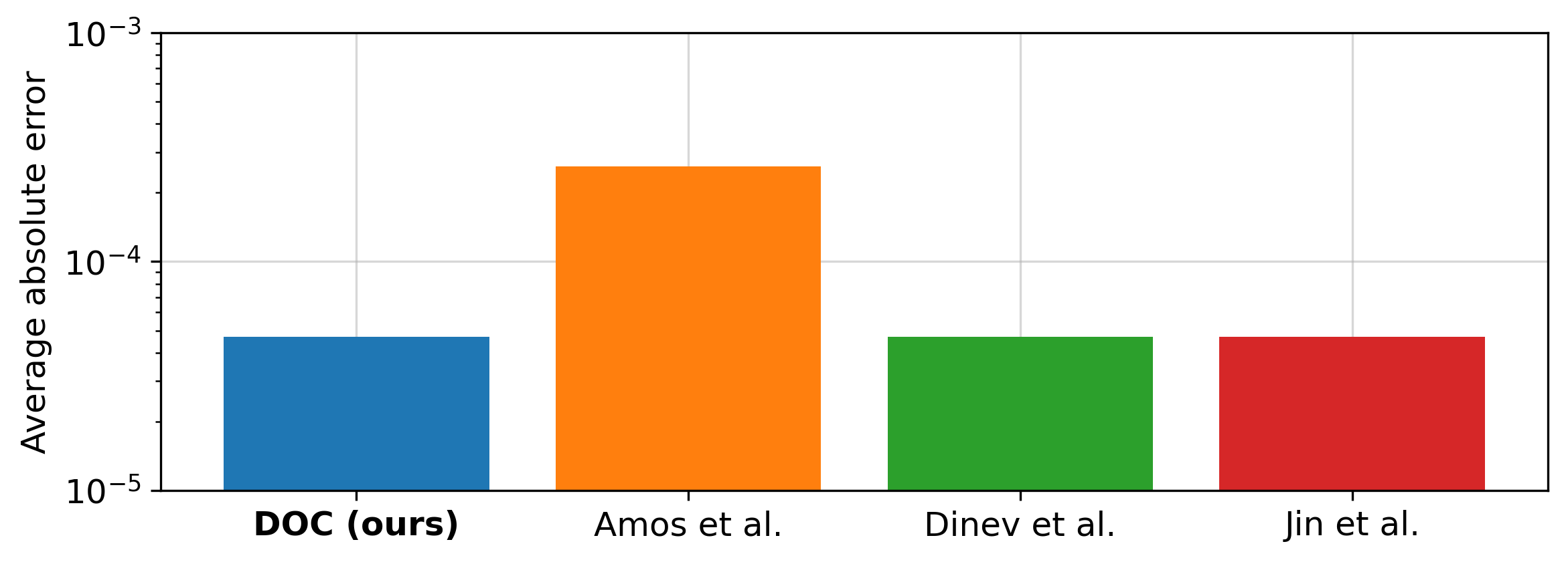
(a) Gradient error comparison. Note the log scale on the y-axis.

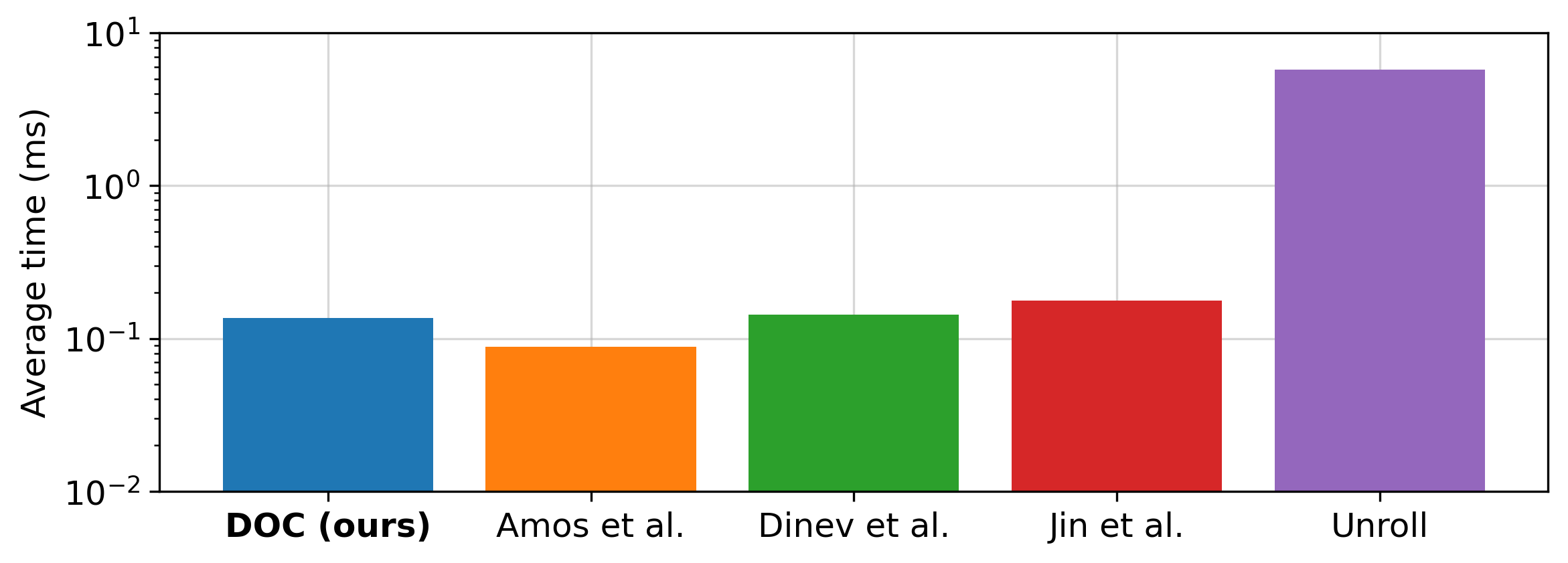
(b) Timing comparison. Note the log scale on the y-axis.

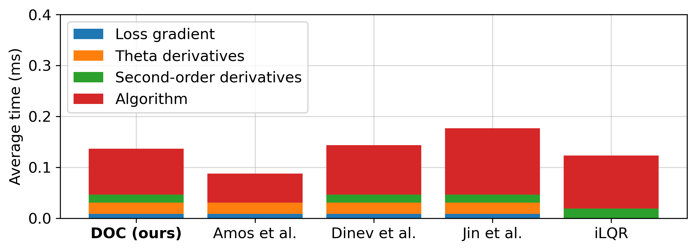
(c) Timing breakdown. iLQR timings are shown for reference.

Figure 7: Dubins vehicle numerical comparisons.

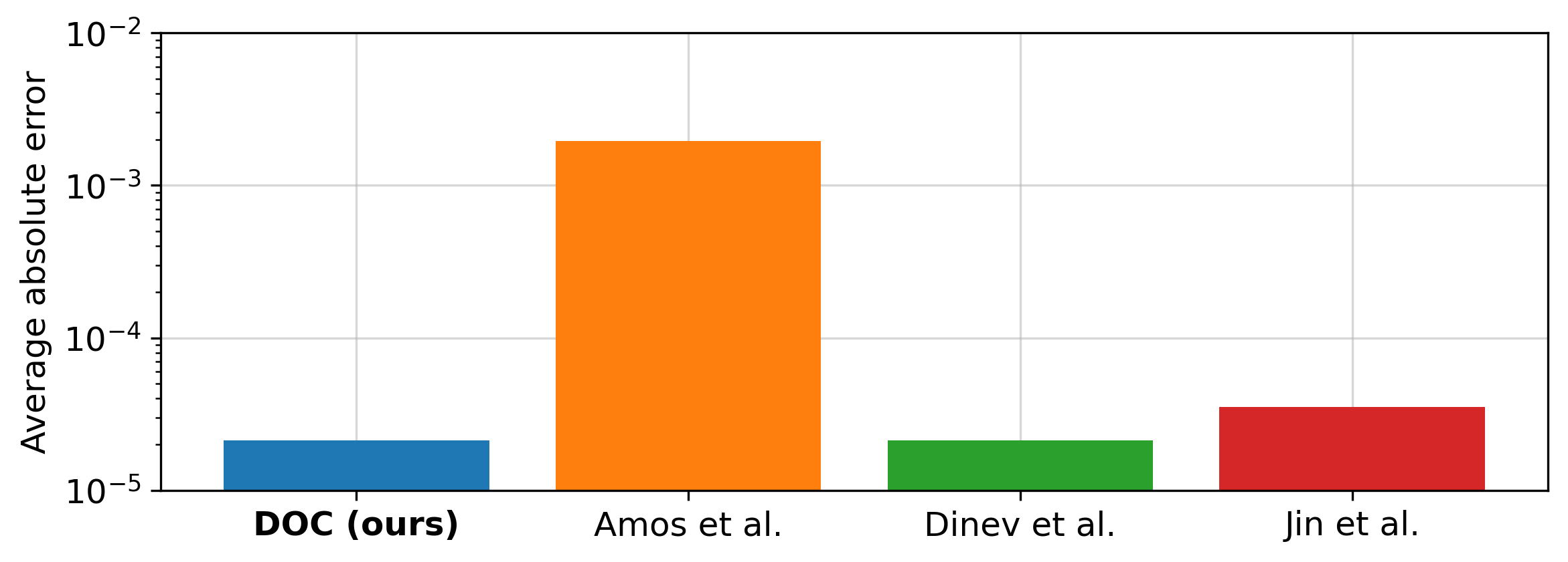
(a) Gradient error comparison. Note the log scale on the y-axis.

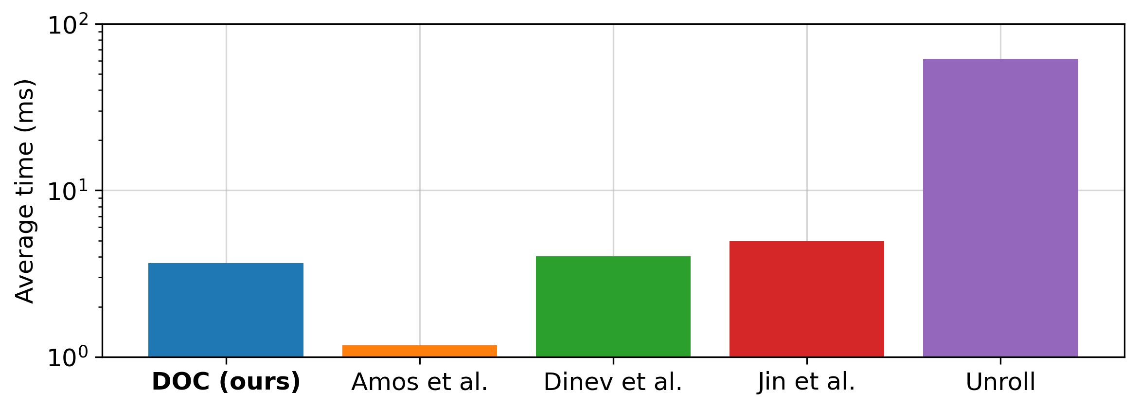
(b) Timing comparison. Note the log scale on the y-axis.

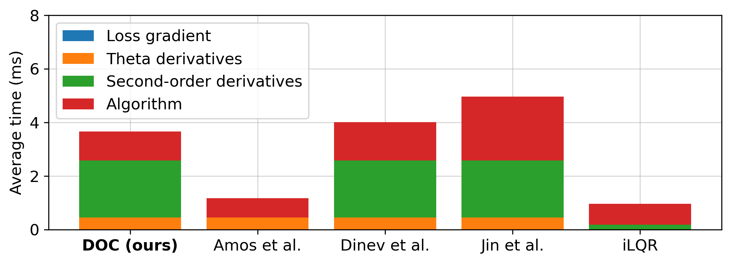
(c) Timing breakdown. iLQR timings are shown for reference.

Figure 8: Quadrotor numerical comparisons.

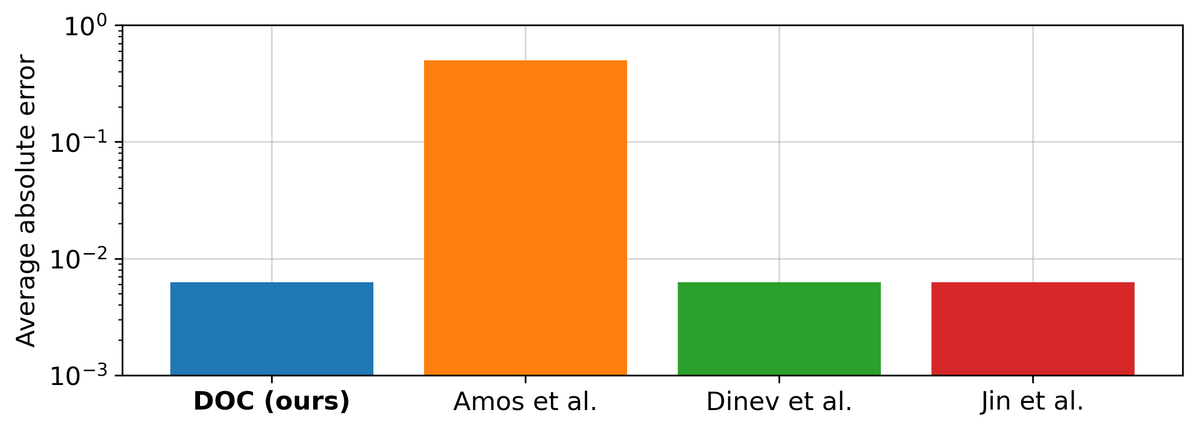
(a) Gradient error comparison. Note the log scale on the y-axis.

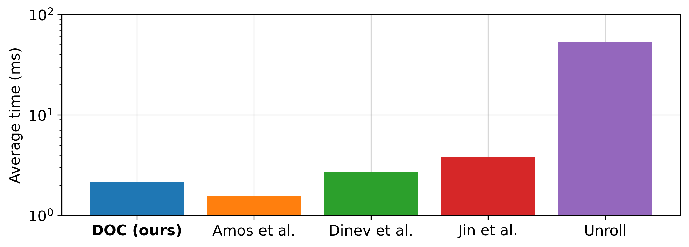
(b) Timing comparison. Note the log scale on the y-axis.

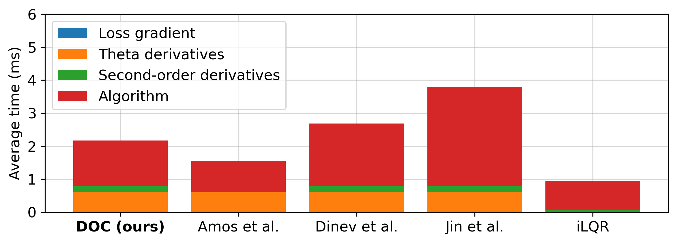
(c) Timing breakdown. iLQR timings are shown for reference.

Figure 9: Robot arm numerical comparisons.

The lower-level control problem is solved using iLQR, and thus only those derivatives are available for reuse by each algorithm. As Amos et al. [5] uses an LQ approximation to the control problem, their algorithm is able to achieve very fast timings. However, this results in inaccurate gradients, which is reflected in the high average absolute error compared to the other methods (see Figs. 7(a), 8(a) and 9(a)).

We highlight the fact that our algorithm is faster, as well as more memory efficient, compared to the work of Dinev et al. [17] due to the smart accumulation of the gradient during the forward pass of Algorithm 1. This prevents needing to store intermediate vectors $\delta{x_{t}}$, etc. The PDP algorithm of Jin et al. [24] produces accurate gradients, but is slower than the other methods due to needing to solve a matrix control system.

Since the MuJoCo dynamics are not compatible with autodiff, comparisons on those systems are omitted. However, we provide a timing comparison between NT-MPC and the proposed DT-MPC on these two systems in Fig. 10. Our proposed method is comparable in runtime with the baseline while vastly improving task performance and safety.

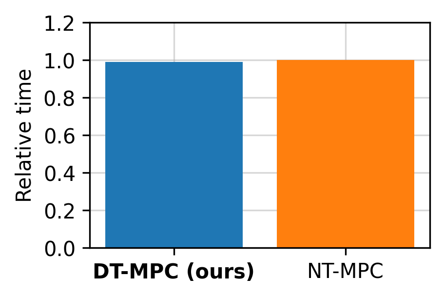
(a) Cheetah system.

(b) Quadruped system.

Figure 10: Timing comparison on MuJoCo systems. Values are normalized with the NT-MPC time corresponding to a value of 1 to show the relative speedup/slowdown of our approach.

Appendix I Further Experimental Detail

This section provides supplementary detail for the experiments performed in Section V. In particular, we define the varying parameterizations of each controller (i.e., what is allowed to adapt during MPC) to highlight the generality of the proposed method.

For both the nominal and ancillary controllers, we use DBaS-DDP [3] and the control-limited DDP solver for handling box control limits [45], dropping the second-order dynamics terms (equivalent to the iLQR approximation). For all experiments, we use the (relaxed) inverse barrier. Additionally, we consider a “computational budget” of 10 iterations. This means NT-MPC can optimize both controllers for the full 10 iterations. However, our method optimizes the lower-level controllers for 9 iterations and uses the last to calculate the parameter gradients as long as either controller converged. Convergence in this sense is declared if the cost does not improve between iterations more than $110-3$.

Of particular note is the choice of learning rate in Algorithm 2. We find that learning rates smaller than $\eta=$110-3$$ tend to suffer in both task completion as well as obstacle avoidance. On the other hand, we have found that a relatively large learning rate of $\eta=$110-2$$ enables fast response to disturbances, especially as the system approaches an obstacle. To improve the efficiency of the method, we adopt a Nesterov momentum scheme [35], but it should be noted that vanilla gradient descent works well in practice.

For all experiments, the nominal controller has a cost function dependent on the task being solved, while the ancillary controller has the general form $\ell=\left\lVert x_{k}-\bar{x}_{k}\right\rVert_{Q}^{2}+\left\lVert u_{k}-\bar{u}_{k}\right\rVert_{R}^{2}+q_{b}b_{k}^{2}$ and $\phi=\left\lVert x_{N}-\bar{x}_{N}\right\rVert_{Q}^{2}+q_{b}b_{N}^{2}$, with weights generally initialized to all ones. To avoid invalid control solutions (i.e., for DDP $R$ must be positive definite), we constrain the parameters (when applicable) through projected gradient descent to ensure: $Q_{ii}\geq 0$, $R_{ii}\geq$110-4$$, ${q_{b}\in[0,1]}$, $\gamma\in[-1,1]$, and $\alpha\geq 0$.

I-A Dubins Vehicle

The Dubins vehicle is a nonlinear system with three states (xy position and yaw angle $\theta$) and two controls (linear velocity $v$ and angular velocity $\omega$). The controls are constrained such that $|v|~{}\leq$ $10\text{\,}\mathrm{m}\text{\,}{\mathrm{s}}^{-1}$ and $|\omega|~{}\leq~{}\pi$ $\text{\,}\mathrm{rad}\text{\,}{\mathrm{s}}^{-1}$. The dynamics are discretized with a time step of $\Delta t=0.01$. The controller horizon is $N=50$ corresponding to a planning horizon of $0.5\text{\,}\mathrm{s}$ long. The task is run for $H=300$ time steps, or until success or failure occurs. Success in Table I is defined as arriving within a $0.25\text{\,}\mathrm{m}$ circle of the target, while failure is defined as colliding with an obstacle.

The nominal cost is fixed and given by $\bar{\ell}=\left\lVert x_{k}-x_{\text{target}}\right\rVert_{\bar{Q}}^{2}+\left\lVert u_{k}\right\rVert_{\bar{R}}^{2}+\bar{q}_{b}b_{k}^{2}$ and $\bar{\phi}=\left\lVert x_{N}-x_{\text{target}}\right\rVert_{\bar{Q}_{f}}^{2}+\bar{q}_{b}b_{N}^{2}$, where ${x_{\text{target}}=(10,10,\pi/4)}$, ${\bar{Q}=\operatorname{diag}(1,1,0)}$, ${\bar{R}=\operatorname{diag}(1,1)}$, ${\bar{Q}_{f}=\operatorname{diag}(1000,1000,1000)}$, $\bar{q}_{b}=1$. The ancillary cost is initialized to all ones and allowed to adapt through minimization of Eq. 9. For this experiment, we use the inverse barrier (relaxed inverse barrier with $\alpha=0$) and fix $\gamma=0$.

I-B Quadrotor

The obstacle field in Fig. 2 is generated as follows. 30 spherical obstacles are created by sampling a center point from the range $[0,10]$ $\text{\,}\mathrm{m}$ in all three axes and a radius from the range $[0.5,1.5]$ $\text{\,}\mathrm{m}$. An additional obstacle with radius $1.5\text{\,}\mathrm{m}$ is placed at the center point $(5,5,5)$ $\text{\,}\mathrm{m}$ between the origin and the target to avoid trivial solutions.

Success for this task is defined as arriving within a $0.5\text{\,}\mathrm{m}$ sphere of the target, while failure is defined as colliding with an obstacle or leaving the bounds $[-2,12]$ $\text{\,}\mathrm{m}$ in any of the three axes.

The dynamics model is adapted from Sabatino [43] and contains 12 states — xyz position, orientation expressed as Euler angles, and linear and angular velocities — and four controls — thrust magnitude and pitching moments. For simplicity, unity parameters ($1\text{\,}\mathrm{kg}$ mass, identity inertia matrix, etc.) are adopted. The thrust is limited to the range $[0,50]$ $\text{\,}\mathrm{N}$ and the pitching moments to $[-10,10]$ $\text{\,}\mathrm{N}\text{\,}\mathrm{m}$. The dynamics are discretized with $\Delta t=0.02$ and the MPC horizon is $N=50$ for both controllers corresponding to a $1\text{\,}\mathrm{s}$ planning horizon. The task is run for $H=300$ time steps, or until success or failure occurs.

Similar to the Dubins vehicle experiment, the nominal cost is fixed and given by $\bar{\ell}=\left\lVert x_{k}-x_{\text{target}}\right\rVert_{\bar{Q}}^{2}+\left\lVert u_{k}\right\rVert_{\bar{R}}^{2}+\bar{q}_{b}b_{k}^{2}$ and $\bar{\phi}=\left\lVert x_{N}-x_{\text{target}}\right\rVert_{\bar{Q}_{f}}^{2}+\bar{q}_{b}b_{N}^{2}$, where $\bar{Q}=\operatorname{diag}(\operatorname{ones}(12))$, $\bar{R}=\operatorname{diag}(\operatorname{ones}(4))$, $\bar{Q}_{f}=1000*\operatorname{diag}(\operatorname{ones}(12))$, and $\bar{q}_{b}=1$. The target state is $x_{\text{target}}=(10,10,10,0,0,0,0,0,0,0,0,0)$. The ancillary cost is initialized to all ones and adapted online through minimization of Eq. 9. The inverse barrier (relaxed inverse barrier with $\alpha=0$) is used and $\gamma=0$ is fixed.

I-C Robot Arm

This system has 12 states corresponding to the orientation $\theta$ (pitch and yaw angles) and angular velocities $\dot{\theta}$ of each of the sections of the arm, and six controls corresponding to the torques $\ddot{\theta}$ applied at each joint. The torques are limited to $|\ddot{\theta}|\leq 10$ $\text{\,}\mathrm{N}\text{\,}\mathrm{m}$. The three links of the arm have lengths $1\text{\,}\mathrm{m}$, $1.5\text{\,}\mathrm{m}$, and $1\text{\,}\mathrm{m}$, respectively. The obstacles visualized in Fig. 4 are fixed with centers $(1,0)$, $(1,1.5)$, $(1,-1.5)$, $(2,-2)$, and $(2,2)$ $\text{\,}\mathrm{m}$, each with radius $0.5\text{\,}\mathrm{m}$ — a $0.5\text{\,}\mathrm{m}$ gap exists on either side of the central obstacle that the arm can safely pass through. At the start of each trial, the arm begins in a random feasible starting orientation which is generated by sampling angles from the range $[-\pi,\pi]$ $\text{\,}\mathrm{rad}$ and rejecting configurations with the arm below the xy-plane or conflicting with obstacles.

The dynamics are discretized with a time step of $\Delta t=0.02$, and the MPC time horizon for both controllers is 50 time steps, corresponding to a $1\text{\,}\mathrm{s}$ planning horizon. The task is run for at most $H=400$ time steps, or until success (the end effector enters a $0.25\text{\,}\mathrm{m}$ sphere of the target location) or failure (any link of the arm collides with an obstacle or the arm goes below the xy-plane) occurs.

The nominal cost function here is reparameterized in terms of the end effector position $e_{k}$. The running cost is given as $\bar{\ell}=\left\lVert e_{k}-e_{\text{target}}\right\rVert_{\bar{Q}}^{2}+\left\lVert u_{k}\right\rVert_{\bar{R}}^{2}+\bar{q}_{b}b_{k}^{2}$ and the terminal cost $\bar{\phi}=\left\lVert e_{N}-e_{\text{target}}\right\rVert_{\bar{Q}_{f}}^{2}+\bar{q}_{b}b_{N}^{2}$, with $\bar{Q}=100*\operatorname{diag}(\operatorname{ones}(3))$, $\bar{R}=100*\operatorname{diag}(\operatorname{ones}(6))$, $\bar{Q}_{f}=10000*\operatorname{diag}(\operatorname{ones}(3))$, $\bar{q}_{b}=$110-3$$, and $e_{\text{target}}=(2,0,1)$. The ancillary cost is the same as described previously and initialized to all ones, except for the barrier weight which is initialized as $q_{b}=$110-3$$.

I-D Cheetah

The cheetah system has 18 states and 6 controls with $\Delta t=0.01$ and control limits $u_{i}\in[-1,1]$. The controller plans for $N=50$ time steps with an allotted task time of $H=300$. The nominal cost is given as $\bar{\ell}=\bar{q}(p_{x}^{(k)}-5)^{2}+\left\lVert u_{k}\right\rVert_{\bar{R}}^{2}+\bar{q}_{b}b_{k}^{2}$ and $\bar{\phi}=\bar{q}_{f}(p_{x}^{(N)}-5)^{2}+\bar{q}_{b}b_{N}^{2}$, where $p_{x}^{(k)}$ is the x-position at time $k$, and $\bar{q}=1$, $\bar{R}=0.01*\operatorname{diag}(\operatorname{ones}(6))$, $\bar{q}_{f}=100$, and $q_{b}=1$. Notably, we fix the terminal cost but allow the remaining parameters to adapt online during MPC — this allows the DT-MPC to improve the task completion percentage without sacrificing safety. The ancillary controller is initialized to all ones. Additionally, we use the relaxed barrier with initialization $\gamma=0,\alpha=0.1$ and allow the parameters to adapt along with the cost function weights. The use of the relaxed barrier here is beneficial as small violations of the pitch angle constraint are acceptable as long as the cheetah does not flip over. As stated in the main text, the loss for both controllers is $L=\left\lVert\bm{p}_{x}^{*}-\bar{\bm{p}}_{x}\right\rVert_{2}^{2}+\left\lVert\bm{b}^{*}\right\rVert_{2}^{2}$, motivating safe task completion.

I-E Quadruped

The quadruped system is a complex robotic system with 56 states and 12 controls. Each leg is a simplified biological model with an extending/contracting tendon. The controls for each leg consist of the yaw angle, lift, and extension of the leg. The dynamics are discretized with $\Delta t=0.005$ and the MPC horizon is $N=50$. The task is run for $H=400$ time steps.

The nominal cost is similar to the cheetah experiment, with $\bar{\ell}=\bar{q}(p_{x}^{(k)}-2.5)^{2}+\left\lVert u_{k}\right\rVert_{\bar{R}}^{2}+\bar{q}_{b}b_{k}^{2}$ and $\bar{\phi}=\bar{q}_{f}(p_{x}^{(N)}-2.5)^{2}+\bar{q}_{b}b_{N}^{2}$, and the weights given as $\bar{q}=1$, $\bar{R}=0.01*\operatorname{diag}(\operatorname{ones}(6))$, $\bar{q}_{f}=100$, and $q_{b}=1$. The ancillary cost is initialized to all ones, except the barrier weight which is initialized to $q_{b}=0.1$. The relaxed inverse barrier is adopted here with initial parameters $\gamma=0,\alpha=1.0$, and both controllers minimize the loss $L=\left\lVert\bm{p}_{x}^{*}-\bar{\bm{p}}_{x}\right\rVert_{2}^{2}+\left\lVert\bm{b}^{*}\right\rVert_{2}^{2}$ for adaptation.

References

- Allan et al. [2017] Douglas A Allan, Cuyler N Bates, Michael J Risbeck, and James B Rawlings. On the inherent robustness of optimal and suboptimal nonlinear MPC. Systems & Control Letters, 106:68–78, 2017.
- Almubarak et al. [2021] Hassan Almubarak, Nader Sadegh, and Evangelos A Theodorou. Safety embedded control of nonlinear systems via barrier states. IEEE Control Systems Letters, 6:1328–1333, 2021.
- Almubarak et al. [2022] Hassan Almubarak, Kyle Stachowicz, Nader Sadegh, and Evangelos A Theodorou. Safety embedded differential dynamic programming using discrete barrier states. Robotics and Automation Letters, 7(2):2755–2762, 2022.
- Amos and Kolter [2017] Brandon Amos and J Zico Kolter. Optnet: Differentiable optimization as a layer in neural networks. In International Conference on Machine Learning, pages 136–145. PMLR, 2017.
- Amos et al. [2018] Brandon Amos, Ivan Jimenez, Jacob Sacks, Byron Boots, and J Zico Kolter. Differentiable MPC for end-to-end planning and control. Advances in Neural Information Processing Systems, 31, 2018.
- Bai et al. [2019] Shaojie Bai, J Zico Kolter, and Vladlen Koltun. Deep equilibrium models. Advances in Neural Information Processing Systems, 32, 2019.
- Bellman [1966] Richard Bellman. Dynamic programming. Science, 153(3731):34–37, 1966.
- Bertrand et al. [2020] Quentin Bertrand, Quentin Klopfenstein, Mathieu Blondel, Samuel Vaiter, Alexandre Gramfort, and Joseph Salmon. Implicit differentiation of lasso-type models for hyperparameter optimization. In International Conference on Machine Learning, pages 810–821. PMLR, 2020.
- Bhardwaj et al. [2020] Mohak Bhardwaj, Byron Boots, and Mustafa Mukadam. Differentiable gaussian process motion planning. In International Conference on Robotics and Automation, pages 10598–10604. IEEE, 2020.
- Blondel et al. [2022] Mathieu Blondel, Quentin Berthet, Marco Cuturi, Roy Frostig, Stephan Hoyer, Felipe Llinares-López, Fabian Pedregosa, and Jean-Philippe Vert. Efficient and modular implicit differentiation. Advances in Neural Information Processing Systems, 35:5230–5242, 2022.
- Bolte et al. [2021] Jérôme Bolte, Tam Le, Edouard Pauwels, and Tony Silveti-Falls. Nonsmooth implicit differentiation for machine-learning and optimization. Advances in Neural Information Processing Systems, 34:13537–13549, 2021.
- Bradbury et al. [2018] James Bradbury, Roy Frostig, Peter Hawkins, Matthew James Johnson, Chris Leary, Dougal Maclaurin, George Necula, Adam Paszke, Jake VanderPlas, Skye Wanderman-Milne, and Qiao Zhang. JAX: composable transformations of Python+NumPy programs, 2018. URL http://github.com/google/jax.
- Buckner and Lampariello [2018] Caroline Buckner and Roberto Lampariello. Tube-based model predictive control for the approach maneuver of a spacecraft to a free-tumbling target satellite. In Annual American Control Conference (ACC), pages 5690–5697. IEEE, 2018.
- Cho et al. [2023] Minsu Cho, Yeongseok Lee, and Kyung-Soo Kim. Model predictive control of autonomous vehicles with integrated barriers using occupancy grid maps. IEEE Robotics and Automation Letters, 8(4):2006–2013, 2023.
- de Oliveira [2012] Oswaldo Rio Branco de Oliveira. The implicit and the inverse function theorems: Easy proofs. arXiv preprint arXiv:1212.2066, 2012.
- Di Cairano and Kolmanovsky [2018] Stefano Di Cairano and Ilya V Kolmanovsky. Real-time optimization and model predictive control for aerospace and automotive applications. In American Control Conference (ACC), pages 2392–2409. IEEE, 2018.
- Dinev et al. [2022] Traiko Dinev, Carlos Mastalli, Vladimir Ivan, Steve Tonneau, and Sethu Vijayakumar. Differentiable optimal control via differential dynamic programming. arXiv preprint arXiv:2209.01117, 2022.
- Eren et al. [2017] Utku Eren, Anna Prach, Başaran Bahadır Koçer, Saša V Raković, Erdal Kayacan, and Behçet Açıkmeşe. Model predictive control in aerospace systems: Current state and opportunities. Journal of Guidance, Control, and Dynamics, 40(7):1541–1566, 2017.
- Feller and Ebenbauer [2016] Christian Feller and Christian Ebenbauer. Relaxed logarithmic barrier function based model predictive control of linear systems. IEEE Transactions on Automatic Control, 62(3):1223–1238, 2016.
- Franceschi et al. [2018] Luca Franceschi, Paolo Frasconi, Saverio Salzo, Riccardo Grazzi, and Massimiliano Pontil. Bilevel programming for hyperparameter optimization and meta-learning. In International Conference on Machine Learning, pages 1568–1577. PMLR, 2018.
- Giftthaler et al. [2018] Markus Giftthaler, Michael Neunert, Markus Stäuble, Jonas Buchli, and Moritz Diehl. A family of iterative gauss-newton shooting methods for nonlinear optimal control. In 2018 IEEE/RSJ International Conference on Intelligent Robots and Systems (IROS), pages 1–9. IEEE, 2018.
- Grandia et al. [2023] Ruben Grandia, Farbod Farshidian, Espen Knoop, Christian Schumacher, Marco Hutter, and Moritz Bächer. DOC: Differentiable optimal control for retargeting motions onto legged robots. ACM Transactions on Graphics (TOG), 42(4):1–14, 2023.
- Jacobson and Mayne [1970] David H Jacobson and David Q Mayne. Differential dynamic programming. Elsevier Publishing Company, 1970.
- Jin et al. [2020] Wanxin Jin, Zhaoran Wang, Zhuoran Yang, and Shaoshuai Mou. Pontryagin differentiable programming: An end-to-end learning and control framework. Advances in Neural Information Processing Systems, 33:7979–7992, 2020.
- Krantz and Parks [2002] Steven George Krantz and Harold R Parks. The Implicit Function Theorem: History, Theory, and Applications. Springer Science & Business Media, 2002.
- Li and Todorov [2004] Weiwei Li and Emanuel Todorov. Iterative linear quadratic regulator design for nonlinear biological movement systems. In First International Conference on Informatics in Control, Automation and Robotics, volume 2, pages 222–229. SciTePress, 2004.
- Limón et al. [2010] Daniel Limón, Ignacio Alvarado, TEFC Alamo, and Eduardo F Camacho. Robust tube-based MPC for tracking of constrained linear systems with additive disturbances. Journal of Process Control, 20(3):248–260, 2010.
- Lorraine et al. [2020] Jonathan Lorraine, Paul Vicol, and David Duvenaud. Optimizing millions of hyperparameters by implicit differentiation. In International Conference on Artificial Intelligence and Statistics, pages 1540–1552. PMLR, 2020.
- Malyuta et al. [2021] Danylo Malyuta, Yue Yu, Purnanand Elango, and Behçet Açıkmeşe. Advances in trajectory optimization for space vehicle control. Annual Reviews in Control, 52:282–315, 2021.
- Mammarella et al. [2019] Martina Mammarella, Dae Young Lee, Hyeongjun Park, Elisa Capello, Matteo Dentis, and Giorgio Guglieri. Attitude control of a small spacecraft via tube-based model predictive control. Journal of Spacecraft and Rockets, 56(6):1662–1679, 2019.
- Mayne [1966] David Mayne. A second-order gradient method for determining optimal trajectories of non-linear discrete-time systems. International Journal of Control, 3(1):85–95, 1966.
- Mayne [2014] David Q Mayne. Model predictive control: Recent developments and future promise. Automatica, 50(12):2967–2986, 2014.
- Mayne et al. [2011a] David Q Mayne, Eric C Kerrigan, and Paola Falugi. Robust model predictive control: Advantages and disadvantages of tube-based methods. IFAC Proceedings Volumes, 44(1):191–196, 2011a.
- Mayne et al. [2011b] David Q Mayne, Erric C Kerrigan, EJ Van Wyk, and Paola Falugi. Tube-based robust nonlinear model predictive control. International Journal of Robust and Nonlinear Control, 21(11):1341–1353, 2011b.
- Nesterov [2003] Yurii Nesterov. Introductory Lectures on Convex Optimization: A Basic Course, volume 87. Springer Science & Business Media, 2003.
- Okada et al. [2017] Masashi Okada, Luca Rigazio, and Takenobu Aoshima. Path integral networks: End-to-end differentiable optimal control. arXiv preprint arXiv:1706.09597, 2017.
- Pannocchia et al. [2011] Gabriele Pannocchia, James B Rawlings, and Stephen J Wright. Conditions under which suboptimal nonlinear MPC is inherently robust. Systems & Control Letters, 60(9):747–755, 2011.
- Petersen and Tempo [2014] Ian R Petersen and Roberto Tempo. Robust control of uncertain systems: Classical results and recent developments. Automatica, 50(5):1315–1335, 2014.
- Poignet and Gautier [2000] Ph Poignet and Maxime Gautier. Nonlinear model predictive control of a robot manipulator. In International Workshop on Advanced Motion Control, pages 401–406. IEEE, 2000.
- Qin and Badgwell [2003] S Joe Qin and Thomas A Badgwell. A survey of industrial model predictive control technology. Control Engineering Practice, 11(7):733–764, 2003.
- Rajeswaran et al. [2019] Aravind Rajeswaran, Chelsea Finn, Sham M Kakade, and Sergey Levine. Meta-learning with implicit gradients. Advances in Neural Information Processing Systems, 32, 2019.
- Rawlings et al. [2017] James Blake Rawlings, David Q Mayne, and Moritz Diehl. Model Predictive Control: Theory, Computation, and Design, volume 2. Nob Hill Publishing Madison, WI, 2017.
- Sabatino [2015] Francesco Sabatino. Quadrotor control: Modeling, nonlinear control design, and simulation. Master’s thesis, KTH Royal Institute of Technology, 2015.
- Safonov [2012] Michael G Safonov. Origins of robust control: Early history and future speculations. Annual Reviews in Control, 36(2):173–181, 2012.
- Tassa et al. [2014] Yuval Tassa, Nicolas Mansard, and Emo Todorov. Control-limited differential dynamic programming. In 2014 IEEE International Conference on Robotics and Automation (ICRA), pages 1168–1175. IEEE, 2014.
- Todorov and Li [2005] Emanuel Todorov and Weiwei Li. A generalized iterative LQG method for locally-optimal feedback control of constrained nonlinear stochastic systems. In Proceedings of the 2005, American Control Conference, 2005., pages 300–306. IEEE, 2005.
- Todorov et al. [2012] Emanuel Todorov, Tom Erez, and Yuval Tassa. Mujoco: A physics engine for model-based control. In 2012 IEEE/RSJ international conference on intelligent robots and systems, pages 5026–5033. IEEE, 2012.
- Tunyasuvunakool et al. [2020] Saran Tunyasuvunakool, Alistair Muldal, Yotam Doron, Siqi Liu, Steven Bohez, Josh Merel, Tom Erez, Timothy Lillicrap, Nicolas Heess, and Yuval Tassa. dm_control: Software and tasks for continuous control. Software Impacts, 6:100022, 2020. ISSN 2665-9638.
- Wieber [2006] Pierre-Brice Wieber. Trajectory free linear model predictive control for stable walking in the presence of strong perturbations. In International Conference on Humanoid Robots, pages 137–142. IEEE, 2006.
- Williams et al. [2018] Grady Williams, Brian Goldfain, Paul Drews, Kamil Saigol, James M Rehg, and Evangelos A Theodorou. Robust sampling based model predictive control with sparse objective information. In Robotics: Science and Systems, volume 14, page 2018, 2018.