X-PSI Parameter Recovery for Temperature Map Configurations Inspired by PSR J0030+0451

Abstract

In the last few years, the NICER collaboration has provided mass and radius inferences, via pulse profile modeling, for two pulsars: PSR J0030$+$0451 and PSR J0740$+$6620. Given the importance of these results for constraining the equation of state of dense nuclear matter, it is crucial to validate them and test their robustness. We therefore explore the reliability of these results and their sensitivity to analysis settings and random processes, including noise, focusing on the specific case of PSR J0030$+$0451. We use X-PSI, one of the two main analysis pipelines currently employed by the NICER collaboration for mass and radius inferences. With synthetic data that mimic the PSR J0030$+$0451 NICER data set, we evaluate the recovery performances of X-PSI under conditions never tested before, including complex modeling of the thermally emitting neutron star surface. For the test cases explored, our results suggest that X-PSI is capable of recovering the true mass and radius within reasonable credible intervals. This work also reveals the main vulnerabilities of the analysis: a significant dependence on noise and the presence of multi-modal structure in the posterior surface. Noise particularly impacts our sensitivity to the analysis settings and widths of the posterior distributions. The multi-modal structure in the posterior suggests that biases could be present if the analysis is unable to exhaustively explore the parameter space. Convergence testing, to ensure an adequate coverage of the parameter space and a suitable representation of the posterior distribution, is one possible solution to these challenges.

https://www.overleaf.com/project/63331d06041e4510858c5dda

1 Introduction

Millisecond pulsars are incredibly valuable resources for understanding the behaviour of matter at extreme densities. With densities that can reach several times the saturation density in their cores, neutron stars are indeed among the densest objects in our Universe (Lattimer, 2012; Oertel et al., 2017; Baym et al., 2018; Tolos & Fabbietti, 2020; Yang & Piekarewicz, 2020; Hebeler, 2021). The main scientific goal of the payload Neutron Star Interior Composition Explorer (NICER) (Gendreau et al., 2016), installed on the International Space Station, is to probe matter at these otherwise inaccessible conditions to constrain the Equation of State (EoS). It targets millisecond pulsars showing X-ray emission with pulsations. This pulsating X-ray emission is thought to originate from the heat deposited at the magnetic poles by return currents (see e.g., Ruderman & Sutherland, 1975; Arons, 1981; Harding & Muslimov, 2001). The thermal X-rays thus generated carry information about the space-time in which the NS is embedded. Meanwhile the relativistic speed of the NS surface and the atmospheric beaming break the degeneracy between the effects of the NS mass and radius, which can then be inferred through Pulse Profile Modeling (PPM) techniques (see Watts et al., 2016; Watts, 2019; Bogdanov et al., 2019b, 2021, and references therein).

We use the X-ray Pulse Simulation and Inference (X-PSI) (Riley et al., 2023) software package, which is designed to simulate the thermal X-ray emission of MSPs and estimate the model parameter values that allow for a good representation of a specific data set. By adopting sampling software like MultiNest (Feroz & Hobson, 2008; Feroz et al., 2009a, 2019), and more specifically PyMultiNest (Buchner et al., 2014a), X-PSI provides a Bayesian inference framework that allows us to explore the parameter space describing the emission model. Model parameters include those that describe the temperature patterns on the NS surface, observer inclination, distance, interstellar medium, the instrument response and the NS mass and radius.

To establish the reliability of inferences with PPM, it is necessary to carry out parameter recovery simulations, where the analysis pipeline is deployed on synthetic data with known input parameters, to see how well those are recovered. While some parameter recovery simulations using X-PSI have already been reported, (Riley, 2019; Bogdanov et al., 2019b, 2021), there are other crucial aspects of the analysis process that still need to be explored to establish the robustness of previous and current findings: this is the aim of the current paper. In particular we investigate the impact of the Poisson noise present in the data, the analysis settings and the randomness of the sampling, and explore the important role of multi-modal structures in the posterior surface. We also perform parameter recovery simulations for the more complex surface temperature patterns that were identified as the preferred geometry in Riley et al. (2019, hereafter R19).

Parameter estimation in the context of PPM, is a high dimensional problem, requiring a large amount of computational resources. For this reason, in this paper we only focus on simulated data representing models and parameter vectors that can reproduce PSR J0030$+$0451 X-ray data (Bogdanov et al., 2019a). PSR J0030$+$0451 is the first MSP whose emission was analysed and for which results were published by the NICER collaboration (Miller et al. 2019, R19). These publications also present the first mass inferences for an isolated NS. Using X-PSI, R19 found that the NICER data of PSR J0030$+$0451 could be well represented by a NS with a radius of $12.74^{+1.14}_{-1.19}\,\mathrm{km}$, a mass of $1.34^{+0.15}_{-0.16}\,\mathrm{M_{\odot}}$ and two hot spots on the southern hemisphere ( R19, ) . The peculiarity of this latter detail, together with the elongated, arc-shape (according to the X-PSI analysis) of one of these hot spots drew a lot of attention among theorists studying magnetic fields on NSs in general and MSPs in particular. These temperature patterns indeed imply the presence of a complex magnetic field with multipolar structure, in contrast to the classical picture of a centered dipolar magnetic field (see e.g., Bilous et al., 2019; Chen et al., 2020; Kalapotharakos et al., 2021). These first NICER results were also recently confirmed by an external group, which also used the openly available X-PSI software to reproduce those initial PSR J0030$+$0451 analyses (Afle et al., 2023).

The derived mass of PSR J0030$+$0451 also valorises the role of this pulsar for EoS studies. Its relatively standard mass complements the high mass of PSR J0740$+$6620 (Cromartie et al., 2020; Fonseca et al., 2021), the second NICER target whose data and results have been published (Riley et al., 2021; Miller et al., 2021; Salmi et al., 2022).

In Section 2, we summarise our inference analysis. We lay out our main questions and how we address them in Section 3. In Section 4 we show our findings and we discuss them in Section 5. We conclude with final remarks in Section 6.

2 Methodology: X-PSI upgrades

In this work we adopt the same X-PSI framework currently used for NICER analyses. We build on the findings of R19, by applying an improved X-PSI pipeline to simulated data that mimics a slightly revised PSR J0030$+$0451 NICER data set. Detailed analysis of this revised data set, which is derived from the one presented in Bogdanov et al. (2019a), but uses the latest NICER response matrix, is the main subject of Vinciguerra et al. (2023, submitted).

The aim of these two papers is to set a baseline for the analysis of new, larger PSR J0030$+$0451 NICER data set that will soon be available. In particular, here we reflect on the current analysis protocol, adopted within the NICER collaboration, and provide a benchmark to consistently interpret future results concerning PSR J0030$+$0451.

2.1 Brief Outline of X-PSI Inference Analysis

In the following, we briefly outline the main steps of this analysis and the most relevant features following recent X-PSI developments.

NICER registers events (which include photons as well as instrumental noise artefacts) characterised by a well-measured time stamp and a specific pulse-invariant (PI) channel. Each NICER PI channel has a nominal energy band which is related to the real energy of incoming photons through the instrument response. The events registered by NICER are then folded over the spin period of the pulsar of interest ($4.87\,\mathrm{ms}$ in the case of PSR J0030$+$0451) and binned in phases (32 phase bins in past and current NICER analyses). The NICER data analysed with X-PSI thus take the form of event counts per PI channel and phase bin. This data is then compared to simulated data of the same form, through our likelihood function (see Section 2.4.3 and Equation 5 of R19, ).

Simulated data are generated by X-PSI, according to the selected model (see Section 2.3) and parameter vector. The models that we employ use relativistic ray tracing techniques and describe: (i) the emission patterns on the NS surface, how the emitted thermal X-rays interact with (ii) the NS atmosphere (using NSX, Ho & Lai, 2001) and (iii) the surrounding space-time (assuming the Oblate Schwarzschild plus Doppler approximation Morsink et al., 2007), (iv) how they travel through the interstellar medium to the telescope, and (v) how they are registered by the telescope. Every model adopted in our analyses has multiple free variables; they include the mass and radius of the pulsar of interest, which impact the observed data through special and general relativistic effects such as lensing, Doppler shifts and aberration (see Bogdanov et al., 2019b, for more details). Within X-PSI, parameter estimation is then performed in a Bayesian inference framework, where the parameter space is explored by the sampling algorithm MultiNest (Feroz & Hobson, 2008; Feroz et al., 2009a, 2019), specifically PyMultiNest (Buchner et al., 2014b).

2.2 Updates since R19

Since the early publication of the analysis of PSR J0030$+$0451 NICER data set (R19), X-PSI underwent several changes; most of them have already been outlined in Riley et al. (2021). Below we briefly list the most relevant differences compared to the analyses presented in R19 (for more details see Riley et al., 2021).

X-PSI version: in this work for simulations and inference analyses we use X-PSI v0.7.9 (v1.0.0 and v2.0.0 to produce the reported corner plots), an updated version of the package used in R19 (X-PSI v0.1). From version v0.6.0, X-PSI allows multiple rays to come to the telescope from the same point on the NS surface, an effect which operates to create multiple images for a small part of the prior compactness space.

Modeling of the instrument response: as in Riley et al. (2021) and Salmi et al. (2022), we no longer include the Crab as part of our modeling of the instrument response, i.e., in Equation 3 of R19, $\beta_{R19}=0$ (here _R19 indicates parameter definition according to R19). We instead use a single parameter $\beta\,[\mathrm{kpc^{-2}}]=\alpha D^{-2}$, where $D$ is the distance in $\mathrm{kpc}$ and $\alpha$ is the energy independent scaling factor that multiplies the reference response matrix. In our analysis $\alpha$ is the only parameter shaping the effective instrument response ($\mathcal{R}_{ij}=\alpha\mathcal{R}^{\star}_{ij}$, where $\mathcal{R}$ and $\mathcal{R}^{\star}$ are respectively the effective and nominal instrument response for the $i^{th}$ channel and the $j^{th}$ energy interval). Our analysis only depends on $\alpha$ and $D$ through their combination $\beta$, hence the choice of sampling the single parameter $\beta$. The prior on $\beta$ has been constructed using two Gaussian distributions truncated at $\pm 5\sigma$ for $\alpha$ and $D$, respectively centered at $1$ and $0.325\,\mathrm{kpc}$ with scale parameters $\sigma$ set to $0.1$ and $0.009\,\mathrm{kpc}$.

Priors: as in Riley et al. (2021) and Salmi et al. (2022), we adopt isotropic priors (i.e., flat in the cosine) for inclination and colatitudes of the hot spot centers (see Section 2.3 for details concerning the model parameters).

Settings: the range of the NICER PI channels has been limited to $[30,300)$, corresponding to nominal energies of $[0.3-3]\,\mathrm{keV}$, compared to the $[25,300)$ range adopted in the analyses of R19. The energy range included in the applied response matrix is also slightly altered, following the changes in the instrument response (the upper limit on the energy considered is now $3.715\,\mathrm{keV}$, compared to $3.6\,\mathrm{keV}$ in R19). Further differences concern settings and definitions of variables specific to the X-PSI pipeline, which are explicitly listed in the X-PSI version of R19 (https://xpsi-group.github.io/xpsi), such as the resolution setting for light bending $num\_rays$ (now, as in Riley et al. 2021 and Salmi et al. 2022, set to 512, in R19 to 200) .

2.3 X-PSI Models

In X-PSI the shape of a hot spot can be modeled by either one or two overlapping spherical caps. In the latter case, one of the caps entirely dominates the emission of the overlap region, masking completely the other component. Each of these caps emits at a uniform temperature. If the temperature of the prioritised one is set to match the rest of the star (in this work always assumed to be zero), it will mask part of the emission from the other without contributing to hot spot radiation (for simplicity, hereafter we refer to such a cap as the omitting component and to the correspondent ceding cap as the emitting component). In this way we can allow emitting regions with circular, annular and crescent shapes, as well as dual temperatures.

Each hot spot component is modeled with a number of cells constituting a grid in azimuth and colatitude. Despite the discretisation, the emitting area is correctly accounted for by appropriately weighting the edge cells. The radiation emerging from the NS surface is then modeled with rays generated from these cells. Using relativistic ray tracing (we adopt the Oblate Schwarzschild plus Doppler approximation of Morsink et al., 2007), we infer for each of these cells the emission angle required for the ray to reach the observer, given the phase of rotation (leaf) and the specific location of the cell on the NS surface. This in turn determines the intensity received by the observer, estimated at different energies, while also accounting for the temperature and surface gravity of the emitting cell, and the interstellar medium. Through the instrument response, we then estimate the events registered by NICER, to which a background component is also added.

We model the NICER data set of PSR J0030$+$0451 with the thermal emission generated by two non-overlapping hot spots on the NS surface, as assumed in R19. This is motivated by the two distinct pulses characterising the data set of interest (see Figure 1 of R19, ).

2.3.1 X-PSI Settings

X-PSI requires us to set specific run parameters; in the analyses presented in this paper, we follow Riley et al. (2021) and Salmi et al. (2022) and (unless otherwise stated) fix: the square root of the approximate number of cells per hot spot sqrt$\_$num$\_$cells to 32; the square root of the maximum number of cells in the grid describing the hot spot component max$\_$sqrt$\_$num$\_$cells to 64; the phase resolution in the star frame num$\_$leaves to 64; and number of energies at which the specific photon flux is calculated num$\_$energies (defined within the likelihood object) to 128. We refer to runs adopting these settings as high resolution runs. Due to limitation in computational resources, in combination with the different scope of our paper, for the most expensive models we often adopt a low resolution setting, given by: sqrt$\_$num$\_$cells=18, max$\_$sqrt$\_$num$\_$cells=32, num$\_$leaves=32 and num$\_$energies=64. Comparing results with these two different resolution settings allow us to assess their impact on our results and evaluate whether we could reduce the required computational resources without compromising the inference outcomes.

2.3.2 Atmosphere and Interstellar Medium Assumptions

In this work we assume the presence of a fully-ionized NSX hydrogen atmosphere (Ho & Lai, 2001; Ho & Heinke, 2009). To obtain the specific intensity of the radiation field, we interpolate the values registered in a lookup table, where this intensity is precomputed as a function of effective temperature, surface gravity, photon energy and the cosine of emission angle calculated from the surface normal (for more details see Section 2.4.1 of R19, ). The methodology is consistent with the setup of R19 and is mostly motivated by limitation on computational resources (for comments over the validity and limitation of this assumption see Section 4.1.1 of R19, ). However, here as in Riley et al. (2021) and Salmi et al. (2022), we adopt an extended table, including higher values for the surface gravity.
The effect of the interstellar medium is modeled and parametrized with the hydrogen column density $N_{\mathrm{H}}$ as in R19 see in particular Section 2.4.1.

2.3.3 Model Naming Convention and Parameters

Within X-PSI it is possible to adopt models with various levels of complexity to match the data. To assist the reader, in Figure 1 we provide a schematic representation of our naming convention for emission models (see R19, for more details). Each hot spot can be characterised by a single temperature (ST) or two temperatures (dual temperature DT). For this paper we will be interested only in single temperature hot spots. In the simplest case, the hot spot is described by an emitting spherical cap, simply labelled ST. More complicated shapes can be obtained, for a single hot spot, by overlapping two different spherical caps. If one of these components masks the other, the hot spot can assume ring-like or crescent-like shapes. We refer to a hot spot, whose masking spherical cap is not constrained in location (except for the overlapping condition), as protruding single temperature PST. So far the applications of X-PSI have been limited to modeling the emission of two non-overlapping hot spots, that we label as primary and secondary hot spots. If the two hot spots describing the emitting surface pattern of our model can assume the same range of shapes, we add: -S if all the parameters of the two hot spots are dependent on each other; and -U if they are all independent from each other. Otherwise, the two or three letter acronyms of each hot spots, separated by a plus, are used to label the model.

All of the two hot spot models adopted so far for NICER analyses include the parameters reported below (parentheses clarify the components in case where two spherical caps are used to describe a hot spot):

• mass $M\,[\mathrm{M_{\odot}}]$: the mass;

• radius $R_{\mathrm{eq}}\,[\mathrm{km}]$: the equatorial radius;

• distance $D\,[\mathrm{kpc}]$: the distance between the Earth and PSR J0030$+$0451 ;

• inclination $i\,[\mathrm{rad}]$: the angle between the spin axis and line of sight;

• column density $N_{H}\,[\mathrm{cm^{-2}}]$: the neutral hydrogen column density. Following the TBabs model (Wilms et al., 2000, updated in 2016), we derive the abundances of all other attenuating gaseous elements, dust, and grains from the value of $N_{H}$;

• temperature of the (emitting, superseding) primary component $T_{p}\,[\mathrm{K}]$;

• temperature of the (emitting, superseding) secondary component $T_{s}\,[\mathrm{K}]$;

• radius of the (emitting, superseding) primary component $\zeta_{p}\,[\mathrm{rad}]$: the angular opening from the center of the NS to the center of the (emitting, superseding) primary spherical cap and its circumference;

• radius of the (emitting, superseding) secondary component $\zeta_{s}\,[\mathrm{rad}]$: the angular opening from the center of the NS to the center of the (emitting, superseding) secondary spherical cap and its circumference;

• colatitude of the (emitting, superseding) primary component $\theta_{p}\,[\mathrm{rad}]$: the angle between the North pole, defined by the spinning direction through the right-hand rule, of the NS and the center of the (emitting, superseding) primary spherical cap;

• colatitude of the (emitting, superseding) primary component $\theta_{s}\,[\mathrm{rad}]$: the angle between the North pole of the NS and the center of the (emitting, superseding) secondary spherical cap;

• primary phase shift $\phi_{p}\,[\mathrm{cycles}]$: the phase shift of the center of the primary prioritised component (omitting or emitting) compared to the reference phase set by the data;

• secondary phase shift $\phi_{s}\,[\mathrm{cycles}]$: the phase shift of the center of the secondary prioritised component (omitting or emitting) compared to the reference phase set by the data;

• energy-independent scaling factor alpha $\alpha$: which multiplies the reference instrument response (more on this in what follows) 9.

In general, our models suffer from many degeneracies (see Section 2.5 of R19, for more details).

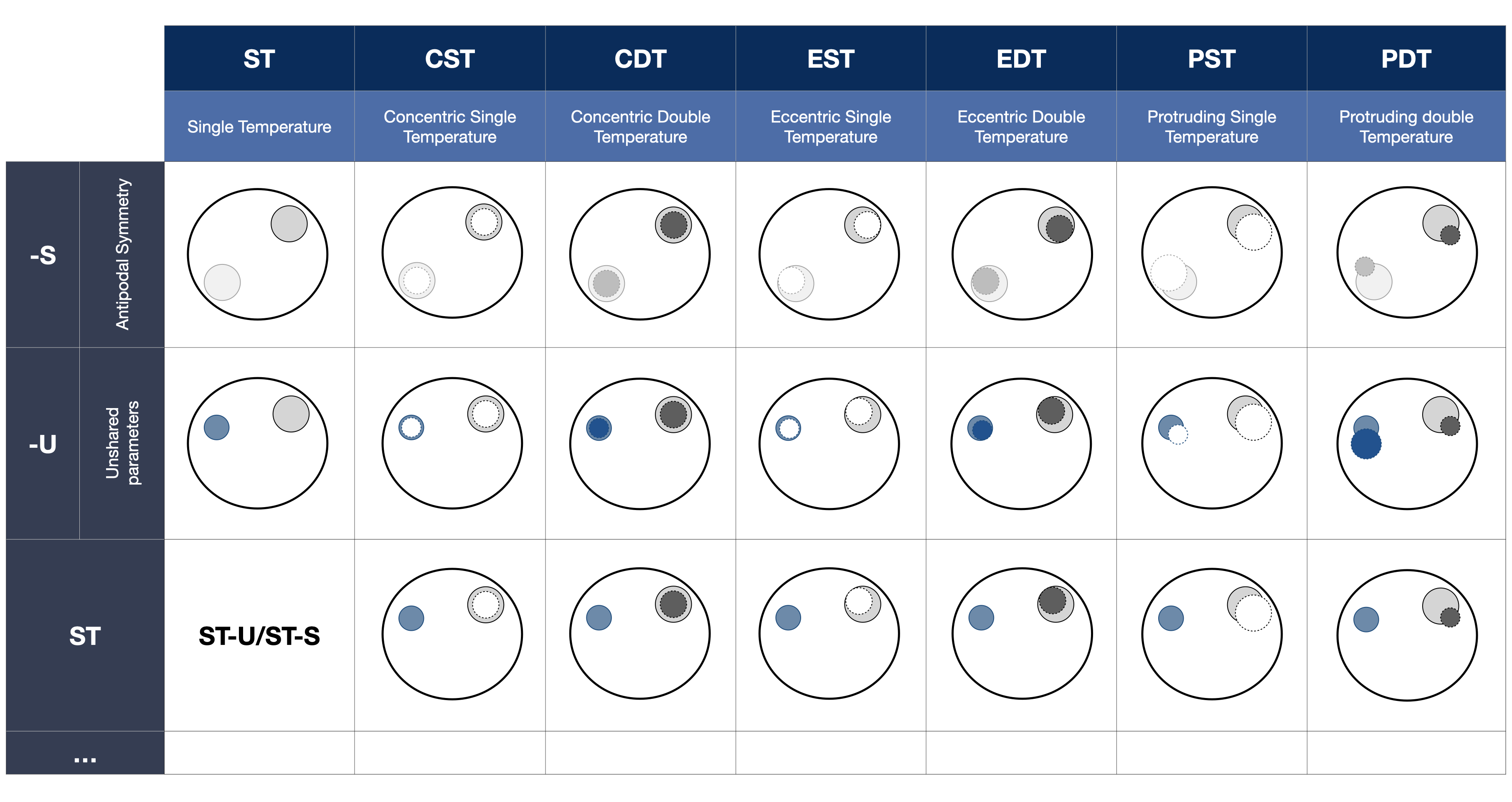
Figure 1: Schematic representation of naming convention adopted within X-PSI. Note that the protruding P configurations include the eccentric E ones which, in turn, include the concentric ones C. In the case of antipodal symmetry (-S in the table), the lightest hot spot indicates that it is located on the hemisphere opposite to the observer. The dots in the last row of the table suggest how additional models could be built, allowing different geometries for the two hot spots.

Motivated by the findings in R19, in this work we apply two different models: ST-U and ST+PST. In R19, ST-U was disfavoured compared to more complex models in view of their correspondent evidences. However this model was not flagged by any anomaly in the residuals (see Section 3, paragraph labeled as Posterior predictive performance in R19) and therefore represents the simplest and least computationally demanding model able to reproduce the PSR J0030$+$0451 NICER data. ST+PST was the preferred and one of the most complex models examined in R19. Below we briefly outline changes in the description of the ST+PST model.

2.3.4 Changes to ST+PST Model Parametrization

According to the naming convention explained above, in the ST+PST model the thermal emission from the NS surface originates from the radiation of a spherical cap with uniform temperature and a second hot spot, whose shape depends on the parameter values determining the relation between an emitting and a masking spherical cap (see also Figure 2). We report parameters as they are defined within the ST+PST model in the X-PSI framework (R19 instead reported derived variables, an alternative description). As in R19, we assume the most complex (PST) hot spot to be the secondary. In this case, the secondary parameters listed above refer to the emitting component of the secondary hot spot, except for the phase, which instead corresponds to the masking region. In addition to the list previously presented, this model requires the definition of the following parameters:

• radius of the masking region of the secondary hot spot $\zeta_{o,s}\,[\mathrm{rad}]$: the angular opening from the center of the NS to the center of the masking spherical cap and its circumference;

• colatitude of the masking region of the secondary hot spot $\theta_{o,s}\,[\mathrm{rad}]$: the angle between the North pole of the NS and the center of the masking spherical cap;

• azimuth offset of the secondary hot spot $\chi_{s}\,[\mathrm{rad}]$: the offset in azimuth between the emitting and the masking spherical caps of the secondary hot spot (the emitting region is taken as a reference).

All the parameters of interest are shown in Figure 2.

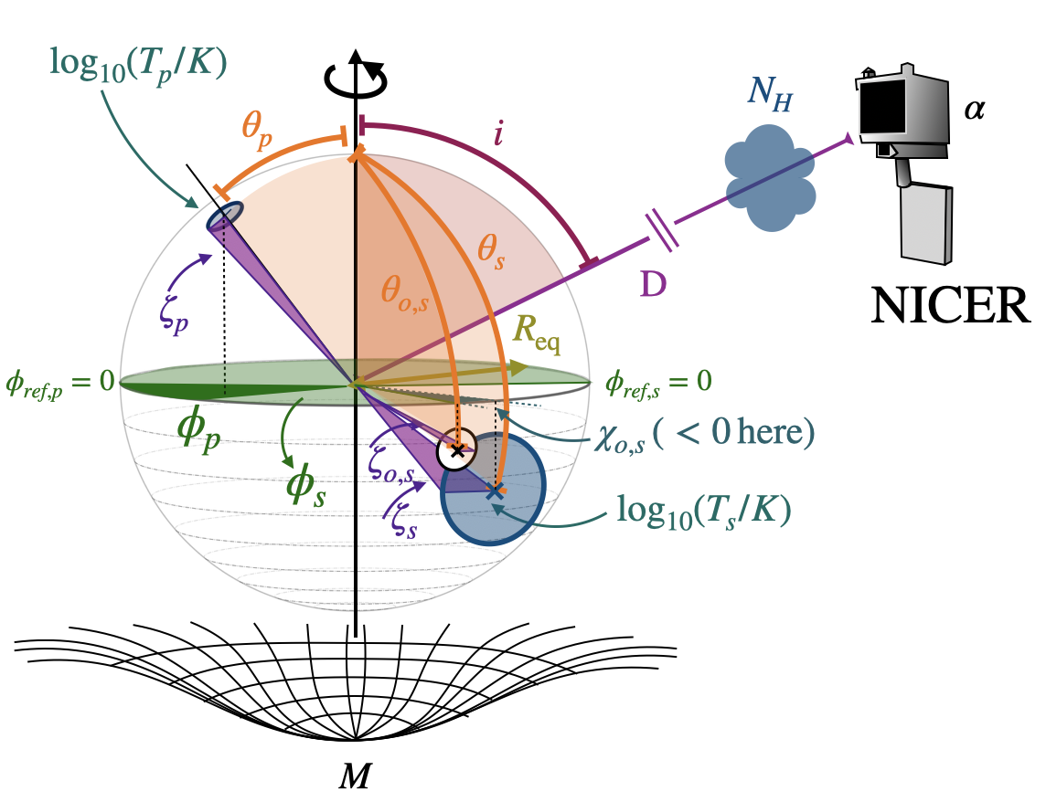
Figure 2: Schematic representation of the ST+PST model and the parameters describing it.

Note that despite the change in the reported variables, our inference analyses are based on the same prior parameterisation described in Section 2.5.6 and Appendix B of R19, except for the following modified rejection rule.

In general in X-PSI, we require that the emitting spherical caps of the two modeled hot spots do not overlap. In R19, the implementation of this condition prevented the primary ST from overlapping also with the omitted part of the emitting spherical cap describing the PST hot spot. There is however no physical reason to exclude such configurations from consideration. Therefore in this work, the primary is allowed to overlap with the secondary masking cap as long as it does not overlap with the non-masked mesh cells of the emitting component, defining a Comprehensive Hot spot prior .

2.4 MultiNest

In our inference runs we use MultiNest to explore the parameter space. Parameter estimation is a by-product of nested sampling algorithms (Skilling, 2004) as MultiNest, which target the computation of the evidence. Conceptually, to perform such calculation, they start from a number of initial samples (live points) that explore the whole prior space and evolve them to define iso-likelihood contours of higher and higher values, enclosing increasingly smaller prior volumes. The process continues until the change of evidence, due to the contribution of the remaining, currently-enclosed prior volume, is estimated to be less than user-defined threshold, which sets the termination condition. Samples are uniformly drawn by MultiNest from a unit hypercube prior volume and are converted to physical parameter values by inverse sampling. X-PSI interfaces with MultiNest through PyMultiNest (Buchner et al., 2014b) by defining priors and the likelihood function. In our analysis, we employ the same background-marginalised likelihood function for phase-folded and binned events described in Equation 4 and 5 of R19 (see also Miller & Lamb, 2015). To probe our parameter space we inverse sample from our priors, as defined in R19 and at the beginning of Section 2.2.

The use of MultiNest requires the definition of a range of settings. In particular in our standard inference runs, we specify the following parameters which can potentially affect the results of our analyses.

• sampling efficiency (SE) $e$ (or equivalently the expansion factor $1/e$): this parameter sets the enlargement factor applied to the prior volume adopted during the sampling procedure (Section 5.2 of Feroz et al., 2009a). This parameter is introduced in MultiNest to widen the prior volume defined by the clusters (ellipsoids), since they may not be optimal in approximating the iso-likelihood contour (suggested values are 0.3 for evidence estimates and 0.8 for parameter estimations). In practice, the value we set in X-PSI is later scaled by the fraction of the unit hypercube sampling space effectively allowed by our prior conditions and rejection rules (see Appendix B Section 5.3 of Riley 2019 for details on its implementation in X-PSI);

• evidence tolerance (ET): this parameter sets our termination criteria (the suggested value is 0.5) by imposing an upper limit over the contribution of the missing prior volume to the evidence at the current iteration (see Appendix A Section 1 of R19, ).

• number of live points (LP): this parameter sets how many samples are initially drawn from the prior volume; these are later replaced following the procedure described in Feroz et al. (2009a) and schematised in Algorithm 1 of the same reference (in Feroz et al. 2009a an example is given with 400 LP, and similar values are reported for UltraNest as well, see Buchner 2021).

• multi-modal or mode-separation method (MM): when this modality is used, the samples associated with the identified modes are evolved independently and locked to the correspondent mode. The number of live points associated with each mode is determined by the prior mass of each mode upon mode separation.

Accuracy and precision of evidence estimates and posterior distributions increase with low sampling efficiency, low evidence tolerance and high number of live points. Whilst making the evidence calculation less efficient, enabling the mode-separation allows us to recover parameters describing disjoint modes identified by MultiNest. The resulting broader understanding of the posterior surface allows us to put the found solutions into a wider context. We can compare them against expectations derived from independent inferences and phenomena e.g. other NICER targets or gravitational wave estimates. Unfortunately the computational cost of the analysis also increases with number of live points, low sampling efficiency and low evidence tolerance. Compromises are therefore required. Below we explore the impact of differences in MultiNest settings on the inferred results, while limiting the computational cost. In particular, we verify the robustness of our inference results employing variations of our reference set up, defined by the same MultiNest setting configuration adopted in most of the analyses of R19: SE 0.3, ET 0.1, LP 1000, MM off.

3 Simulations and Tests: the Case of PSR J0030+0451

3.1 Our Main Lines of Enquiry

This work expands the previous studies reported in Riley (2019) and Bogdanov et al. (2021). In particular we aim to explore the robustness of X-PSI parameter recovery, i.e. checking whether the injected parameter values are recovered within statistically expected credible intervals, for configurations that resemble those emerging both from R19 and a revised PSR J0030$+$0451 data set (Bogdanov et al., 2019a; Vinciguerra et al., 2023, submitted). For this reason we test:

• different Poisson noise realisations;

• different MultiNest and X-PSI settings;

• different initial random conditions in the sampling process;

• different models describing the emission pattern, including the never-before-tested and favored, according to R19, ST+PST model (in particular, data sets are generated and analysed with ST-U and ST+PST models);

• the effect of a mismatch between the model used to generate and analyse the data sets.

Ideally to unveil possible biases, verify the statistical properties of our results and assess their reliability, we would set up large scale simulation studies, exhaustively exploring the posterior distributions inferred from the analysis of the actual data set (Vinciguerra et al., 2023, submitted), similarly to what has been done e.g., in Berry et al. (2015). Through such studies, we could also confirm the expected dependencies of the inference performances on parameter values (Lo et al., 2013, and refs therein). However there is a considerable mismatch between the computational resources available to us and the resources required to carry out such tests. We therefore restrict our study to two simulated expected (i.e., in absence of noise) signals, corresponding to two specific parameter vectors, one per model. With this limitation, we used about $\sim 1.\times 10^{6}$ core-hours on the Dutch national supercomputer Cartesius/Snellius .

3.2 Presentation of Injected Data

Here we describe the simulated signals that we adopt for the inference analyses presented in this work. The simulated data sets can be found in the Zenodo repository Vinciguerra et al. (2023, the Zenodo link will be made public, and the files available, once the publication is accepted ). Using the ST-U model, we produce 7 different data sets; all of them rely on the same expected signal and parameter vector, but incorporate different noise realisations. These are obtained applying Poisson noise, with different random seeds, over the expected counts per channel and phase bin (grouped in $270\times 32$ bins), calculated from the applied model, parameter vector and correspondent background. The exact procedure is explained in detail in the X-PSI tutorial (https://xpsi-group.github.io/xpsi/Modeling.html#Synthesis). The expected signal is fixed by the maximum likelihood sample found by a preliminary ST-U inference run (SE 0.3, ET 0.1, LP 10 000, MM on) on the revised NICER data set of PSR J0030$+$0451 analysed in Vinciguerra et al. (2023, submitted). The posterior sample sets the values of the 13 model parameters outlined in Section 2.3, which in turn determine the simulated thermal emission of PSR J0030$+$0451. These are consistent with the parameter posteriors found by R19. The specific parameter values adopted for simulation in this work are reported in Table 1 and correspond to the geometric configuration reported in the left panel of Figure 3.

Similarly, we generate three different data sets adopting the more complex ST+PST model. We limit our tests to three different Poisson noise realisations, built in the same way as for the ST-U model, since analysing data sets assuming ST+PST is considerably (up to $\sim 90$ times, for the same MultiNest and X-PSI settings) more expensive than when using the ST-U model. These noise realisations are applied on the expected counts obtained given the 16 values of the model parameters reported in the last column of Table 1 and represented as hot spot geometric configuration in the right panel of Figure 3. These values describe the maximum likelihood sample of a preliminary low resolution ST+PST run (SE 0.3, ET 0.1, LP 10 000, MM on) from the revised NICER data set of PSR J0030$+$0451 (Vinciguerra et al., 2023, submitted). This parameter vector resembles the bulk of solutions found by R19 with the same model.

For all data sets, we also fix the 270 parameters (one per PI channel) that we use to model the phase-independent background (see Section 2.4.3 of Riley et al., 2021; Salmi et al., 2022, for more details on background modeling within X-PSI). Since the signal is constructed by folding over the counts collected over many rotational cycles, this background should account for contributions from cosmic energetic particles, X-ray contamination from the Sun, including optical loading, as well as other X-ray point sources in NICER’s field of view (as their time dependence should wash out over in the folding procedure) . The background is chosen to maximise the likelihood of the NICER revised data set being produced by the hot spot emission described by the 13 (for data sets constructed using the ST-U model) or 16 (for data sets constructed using the ST+PST model) parameter values of Table 1.

To produce synthetic data with X-PSI, we adopt the synthesise$\_$given$\_$total$\_$count$\_$number X-PSI function. This calculates a mock data set and its associated exposure time from the values of the model parameters and the number of total counts expected from the source and background.

All the data sets analysed in this work have been generated assuming high resolution in terms of number of cells, leaves and energies (see Section 2.3 for more details).

Table 1: Injected model parameters

Parameter	ST-U value	ST+PST value
$M\,[\mathrm{M_{\odot}}]$	1.13	1.33
$R_{\mathrm{eq}}\,[\mathrm{km}]$	10.20	13.91
$\beta\,[\mathrm{kpc^{-2}}]$	7.19	9.25
$\cos(i)$	0.545	0.766
$N_{H}\,[\mathrm{cm^{-2}}]$	1.40	0.98
$\log_{10}(T_{p}/\mathrm{K})$	6.11	6.10
$\log_{10}(T_{s}/\mathrm{K})$	6.10	6.10
$\zeta_{p}\,[\mathrm{rad}]$	0.15	0.08
$\zeta_{s}\,[\mathrm{rad}]$	0.32	0.89
$\theta_{p}\,[\mathrm{rad}]$	2.45	1.97
$\theta_{s}\,[\mathrm{rad}]$	2.75	2.98
$\phi_{p}\,[\mathrm{cycles}]$	0.46	0.46
$\phi_{s}\,[\mathrm{cycles}]$	0.50	0.24
$\zeta_{o,s}\,[\mathrm{rad}]$	-	0.94
$\theta_{o,s}\,[\mathrm{rad}]$	-	2.98
$\chi_{s}\,[\mathrm{rad}]$	-	-0.70

Note. — Parameters are given in the same format adopted to define our models; in particular we express the information concerning inclination and temperature respectively in the form of cosine $\cos(i)$ and logarithms $\log_{10}(T)$. The reference phase of $\phi_{s}$ is half a cycle away from the reference phase used to define $\phi_{p}$, hence the phase difference between primary and secondary is $\phi_{s}+0.5-\phi_{p}$.

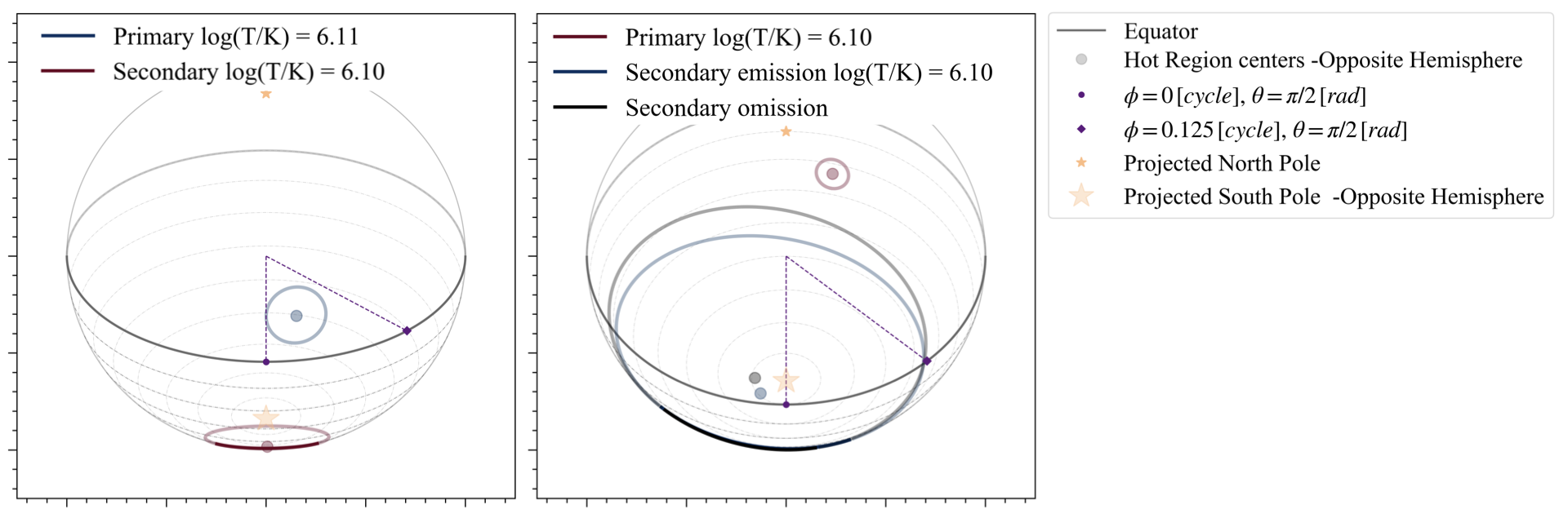
Figure 3: Schematic representation of the geometric configurations, as seen from Earth, of the NS hot spots adopted to create the data analysed in this work. The parameter values corresponding to the ST-U and ST+PST models, respectively shown on the left and right panels, are reported in Table 1. The configurations show, in solid lines, the hot spot section visible to us at phase $\phi=\phi_{p}=0.0$ cycle (the reference phase of the primary hot spot); in transparency we show the component parts on the hemisphere which, at this rotation phase, is opposite to the observer. With a second point on the equator we also display how the NS rotates. The blue/red line is used to mark the hottest/coldest component. We also remind the reader that for the ST-U configuration, the primary hot spot is defined as the component with lower colatitude, while for the ST+PST it is set by the hot spot description as a single spherical cap with uniform temperature.

3.3 Performed Inference Runs

To investigate the robustness of X-PSI inference analyses, we set up a number of inference runs on our simulated data sets. Given our limited computational resources and the overall adequacy of the ST-U model in explaining the PSR J0030$+$0451 NICER data set (see Section 2.3.3), we investigate the various performance dependencies listed in Section 3.1, employing the cheapest ST-U model in the majority of our cases.

3.3.1 Inferences with ST-U Models

All inference runs performed with the ST-U model are carried out with the high resolution X-PSI settings (the same settings used for the data generation) and are reported in Table 2. Below we briefly motivate our ST-U inference runs, in view of the target tests described in Section 3.1.

Noise: To test the effect of different noise realisations in parameter recovery and the width of credible intervals (particularly for the case of mass and radius), we analyse all 7 data sets with the default MultiNest settings.

SE, ET and randomness in the sampling process: Of the 7 data sets built with the ST-U model, we use two to test the effect of different values of SE, ET and variability due to the randomness in the sampling process. Motivated by the settings suggested by the MultiNest authors and what was adopted in R19, we test the SE with additional values SE: 0.1, 0.8, while keeping ET, LP and MM constant at their default and the ET with additional value ET: 0.001, while keeping SE, LP and MM constant at their default. We than repeat all these runs, and the one with the default settings, a second time to test variability due to the randomness in the sampling process.

LP and MM: For the same two data sets selected for testing SE and ET, we also perform an additional inference run, using 10 000 live points and adopting the mode-separation method (MM on) to increase our prior exploration and learn more about our posterior surfaces.

Performance when the data set is created with the more complex ST+PST model: We would also like to understand the impact of adopting a model in our inference analysis which does not include all the complexity of the true (in this case simulated) system. This indeed reflects the situation for our normal NICER analysis, where the models adopted for inference cannot incorporate every detail of the physics describing the actual physical system. However we normally assume that the collected data is not resolved enough for our analyses to be sensitive to the missing physics. So to test how sensitive we are to the hot spot shapes, we use one of the data sets generated employing the ST+PST model, and test the performance of our inference pipeline when assuming the ST-U model. In this case indeed we know that the model adopted for our inference lacks the complexity used to generate the data. In particular we would like to check: if mass and radius can be recovered anyway; if the residuals hint at any inadequacy of the model to reproduce the data; if the evidence helps in identifying ST+PST as the best model (for which we also need an inference run with ST+PST as the assumed model, see below); the relation between the recovered and injected geometrical parameters; and how the identified solutions compare to what was found for ST-U in R19. This test can also highlight degeneracies between models and, as a natural consequence, the presence of multi-modal structure in the posterior surface (since we can consider the different hot spot models as nested). As shown in Table 2, we perform 5 inference runs with different MultiNest settings to check the robustness of our results.

Data set	SE	ET	LP	MM	N	Core hs
Noise 1	0.3	0.1	$10^{3}$	off	2	$\sim$900
						$\sim$1500
	0.1	0.1	$10^{3}$	off	2	$\sim$2900
						$\sim$1800
	0.8	0.1	$10^{3}$	off	2	$\sim$500
						$\sim$1000
	0.3	0.001	$10^{3}$	off	2	$\sim$1700
						$\sim$2000
	0.3	0.1	$10^{4}$	on	1	$\sim$12800
Noise 2	0.3	0.1	$10^{3}$	off	2	$\sim$600
						$\sim$1300
	0.1	0.1	$10^{3}$	off	2	$\sim$1200
						$\sim$3000
	0.8	0.1	$10^{3}$	off	2	$\sim$700
						$\sim$800
	0.3	0.001	$10^{3}$	off	2	$\sim$2000
						$\sim$900
	0.3	0.1	$10^{4}$	on	1	$\sim$13200
Noise 3	0.3	0.1	$10^{3}$	off	1	$\sim$1200
Noise 4	0.3	0.1	$10^{3}$	off	1	$\sim$1400
Noise 5	0.3	0.1	$10^{3}$	off	1	$\sim$700
Noise 6	0.3	0.1	$10^{3}$	off	1	$\sim$800
Noise 7	0.3	0.1	$10^{3}$	off	1	$\sim$1000
ST+PST	0.3	0.1	$10^{3}$	off	1	$\sim$1400
(Noise 1)	0.8	0.1	$10^{3}$	off	1	$\sim$600
	0.1,	0.1	$10^{3}$	off	1	$\sim$2900
	0.3,	0.001	$10^{3}$	off	1	$\sim$1100
	0.3,	0.1	$10^{4}$	on	1	$\sim$13700

Table 2: Summary of the inference runs performed with the ST-U model. High resolution is always used for number of cells, leaves and energies. The first column shows the synthetic data used for the inference run (horizontal lines separate different data sets). The different noise numbers indicate different noise realisations. SE: sampling efficiency; ET: evidence tolerance; LP: live points and MM (multi-mode): mode-separation modality describe the MultiNest settings of the inference run (more details can be found in Section 2.4). N represents the number of repetitions of a run. Core hs indicates the CPU core hours used to perform the inference run; note that when two identical inference analyses have been performed, the CPU core hours for each run are reported in two separate and consecutive rows.

3.3.2 Inferences with ST+PST Models

Because of the high computational costs of inference runs employing the ST+PST model, we often use the low resolution X-PSI settings, reducing the number of leaves, cells and energies compared to what was used to produce the various data sets. This change also allows us to explore the robustness of our results when adopting more limited resolution.

The settings used for ST+PST inference runs and their motivation resemble what is reported in Section 3.3.1 for ST-U runs and they are summarised in Table 3. In addition to the cases presented for ST-U analyses, here we also check the effect of external constraints on parameter recovery and the width of credible intervals. In particular we set up three inference runs assuming that there are tight constraints on mass and distance (for one run), and mass, distance and inclination for the other two. We choose uncertainties compatible with those being used for other NICER sources, where these constraints are available. For these runs, we modify the above-described priors as follows.

Mass prior: We sample the NS mass from a normal distribution, centered on an injected value of $M=1.33\,M_{\odot}$, characterised by standard deviation $\sigma=0.053\,M_{\odot}$ and truncated at $\pm 5\sigma$;

Distance prior: As mentioned at the beginning of Section 2.2, we use information about the distance to define the prior of the $\beta$ parameter. Differently from the other analyses (including what was assumed in R19), for these inference runs we adopt $\sigma=0.0006$ kpc (instead of $\sigma=0.009$ kpc).

Inclination prior: Finally we tighten the prior on inclination, using a truncated normal distribution, with center $\arccos(0.766)$ and $\sigma$ set to $0.0001$, on the inclination and inverse sampling the $\cos(i)$ from the cosine of the cumulative distribution of this function.

Data set	SE	ET	LP	MM	X-PSI settings	constraints	Core hs
Noise 1	0.3	0.1	$10^{3}$	off	LR	NO	$\sim$12100
	0.8	0.1	$10^{3}$	off	LR	NO	$\sim$4700
	0.8	0.1	$5\times 10^{3}$	off	LR	NO	$\sim$11600
	0.3	0.1	$10^{4}$	on	LR	NO	$\sim$ 55500
	0.8	0.1	$10^{3}$	off	HR	NO	$\sim$14600
	0.8	0.1	$6\times 10^{3}$	off	HR	NO	$\sim$103400
	0.8	0.1	$10^{3}$	off	LR	MD	$\sim$3200
	0.8	0.1	$10^{3}$	off	LR	MDI	$\sim$7000
	0.3	0.1	$10^{4}$	off	LR	MDI	$\sim$43700
Noise 2	0.3	0.1	$6\times 10^{3}$	off	LR	NO	$\sim$23000
Noise 3	0.3	0.1	$6\times 10^{3}$	off	LR	NO	$\sim$35500
ST-U	0.8	0.1	$10^{3}$	off	LR	NO	$\sim$3300
(Noise 1)	0.3	0.1	$10^{4}$	on	LR	NO	$\sim$79800

Table 3: Summary of the inference runs performed with the ST+PST model. The first column shows the synthetic data used for the inference run (horizontal lines separate different data sets). The different noise numbers indicate different noise realisations. SE: sampling efficiency; ET: evidence tolerance; LP: live points and MM: mode-separation (multi-mode) modality describe the MultiNest settings of the inference run (more details can be found in Section 2.4). LR and HR respectively correspond to low and high resolution. The seventh (second-to-last) column describes the parameters on which we applied constrained priors: M stands for mass, D for distance and I for inclination. The CPU hours needed for each run are reported in the last column.

4 Results

In this section, we present the overall results of our inference runs. The data and routines (including some examples of modules adopted by X-PSI for inference) necessary to reproduce the posterior distributions presented in this Section are reported in the Zenodo repository Vinciguerra et al. (2023, the Zenodo link will be made public, and the files available, once the publication is accepted ).

Since the main goal of the NICER mission is to measure the masses and radii of neutron stars, we particularly focus on the recovery of these parameters. In this list of fundamental variables, we also include the compactness, the combination of mass and radius to which our analysis is expected to be most sensitive. In Figures 5, 6, 7, 9, 10 and 11 we therefore report the posterior distributions of mass, radius and compactness obtained by X-PSI, when adopting MultiNest to sample the parameter space, and smoothed with Kernel Density Estimations from GetDist . As in R19, Riley et al. (2021); Salmi et al. (2022), in the 1D posterior plots we highlight the area enclosed within the $\sim 16\%$ and $\sim 84\%$ quantiles of the 1D marginalised distribution, while in the 2D plots we show contours for the $\sim 68.3\%$ credible regions; injected values are reported with thin solid black lines. In most of our 2D posterior plots, showing compactness versus radius, the KDE interpolation introduces an artefact at the boundary of the compactness limit, applied through rejection rules in our prior definition (similar rejection rules and artefacts are also present in R19, Riley et al. 2021; Salmi et al. 2022) .

4.1 Inferences with the ST-U Model

We first focus on our ST-U inference runs, whose settings are summarised in Table 2. In particular here we consider parameter estimations on data generated with the same ST-U model (results obtained with mismatching models are reported in Section 4.3).

4.1.1 Noise and Settings

Figures 5, 6 and 7 show that overall mass, radius and compactness are well recovered by our inference runs. This is also demonstrated by the P-P plot reported in Figure 4. The inferred geometry of the hot spots also resembles the correct configuration shown in the left panel of Figure 3. In particular we find that, with our default MultiNest settings, the percentage of parameters recovered withing the 1D 68% credible interval lies within the expected, although indicative, range $\sim(54-84)\%$ , for 5 out of the 7 inference runs characterised by different noise realisations. This range expresses the uncertainty due to the finite and, for statistical purposes, relatively low number of model parameters. The $\sim(54-84)\%$ range is defined by the $\sim 16\%$ and $\sim 84\%$ quantiles of the percent point function of a binomial distribution characterising a sample of size $n=13$ (number of inferred parameters per run, for the ST-U model) and rate of success $p=68\%$ (considered credible interval). Since we calculated this uncertainty also at the 68% level, our findings (i.e., that 5 of 7 runs exhibit parameter recovery within the expected range) are consistent with expectations. The two outliers, generated with noise realisation 4 and 5, recover respectively 12 and 2 of the parameters within the 1D 68% credible interval. Comparing the two panels in Figure 5 and looking at Figure 6, we notice that a major role is played by the noise realisation. In particular, noise seems to have a greater effect than the MultiNest settings on the precision and accuracy of our results. Figure 5 shows, however, that the impact of MultiNest settings is also somewhat dependent on the noise realisation. Indeed the right panel (where the analysed data was subjected to the noise realisation 2) shows a larger scatter in the results compered to the left one (where the analysed data was subjected to the noise realisation 1).

In Figure 6, we notice that the injected values of mass and radius intersect the posterior distributions of the data set labeled with noise realisation 5 only at their tails. Even in this case however, our analysis is able to identify the correct compactness. All of our runs find the injected value of compactness within the 68% credible interval of its 1D posterior distribution, the only exceptions being the runs whose noise realisation is labeled with 2; in these cases the true value lies just outside this boundary.

As mentioned before, the P-P plot of Figure 4 summarises the findings outlined above, focusing on mass, radius and compactness, for the 7 different noise realisations tested with the ST-U model and whose marginalised posteriors are shown in Figure 6. Both plots show that the mass is always underestimated, however it stays well within the 3 $\sigma$ (Cameron, 2011) level. Radius and compactness are well recovered, lying most of the time within the 1 $\sigma$ level.

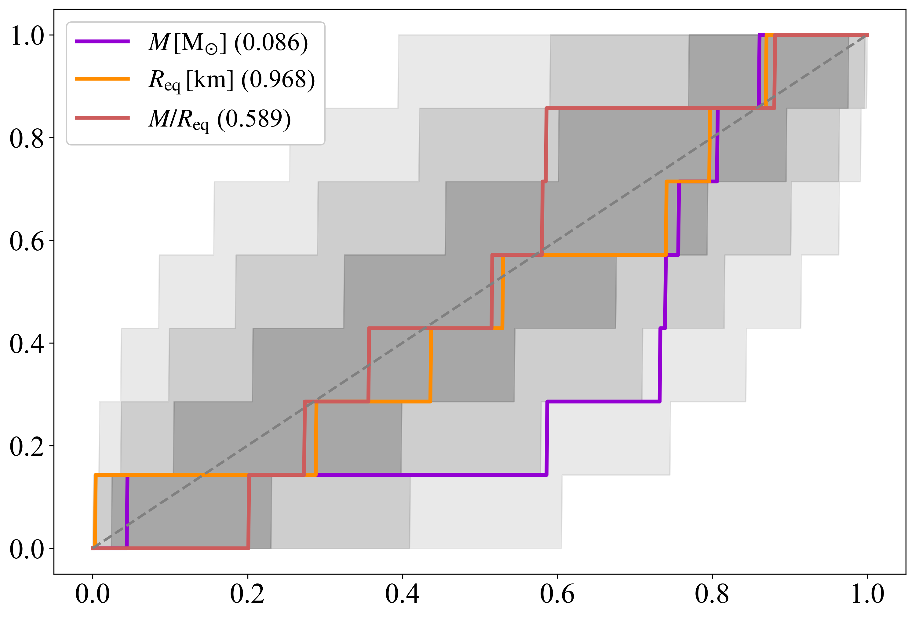
Figure 4: P-P plot for the 7 noise realisations produced and analysed with the ST-U model. It represents, for mass, radius and compactness the cumulative fraction recovered within a credible interval (i.e. the cumulative of the left-side p-value at which the injection is found) as a function of the credible intervals. The legend values in parentheses are the p-values from the KS-test against the theoretical uniform expectations (the injected value should appear $p\%$ of the times within the $p\%$ credible interval). The grey areas represent the 1, 2, and 3 $\sigma$ confidence intervals on the theoretical expectations, calculated according to Cameron (2011).

These findings corroborate the robustness and reliability of our compactness inferences, at least in absence of unaccounted-for physics.

4.1.2 Degeneracies and Posterior Multi-Modal Structure

As shown in Table 2, we also run our inference analyses enabling the mode-separation modality. Thanks to these runs, we have uncovered a multi-modal structure in our likelihood and posterior surfaces, that were not highlighted in the earlier R19 study. We find two distinct modes. In terms of hot spot geometries, these two modes are qualitatively similar to the two leftmost plots in Figure 8. The posteriors of mass, radius and compactness of these two runs, plotted with dashed black lines in Figure 5, correspond to the main mode. In terms of likelihood, there is a clear preference for the main mode; the difference in log-likelihood correspondent to the maximum likelihood samples of these two modes is indeed $\sim 25$. Although the secondary modes, found by the two mode-separation runs (respectively on data generated with noise realisations 1 and 2), share the main characteristics (very low inclination angle, two hot spots similar in size and temperature, almost antipodal in phase, close to the equator and always on the southern hemisphere), they present slightly different properties. In particular, the posterior distributions of the NS mass and radius have different averages and standard deviations as reported in Table 4.

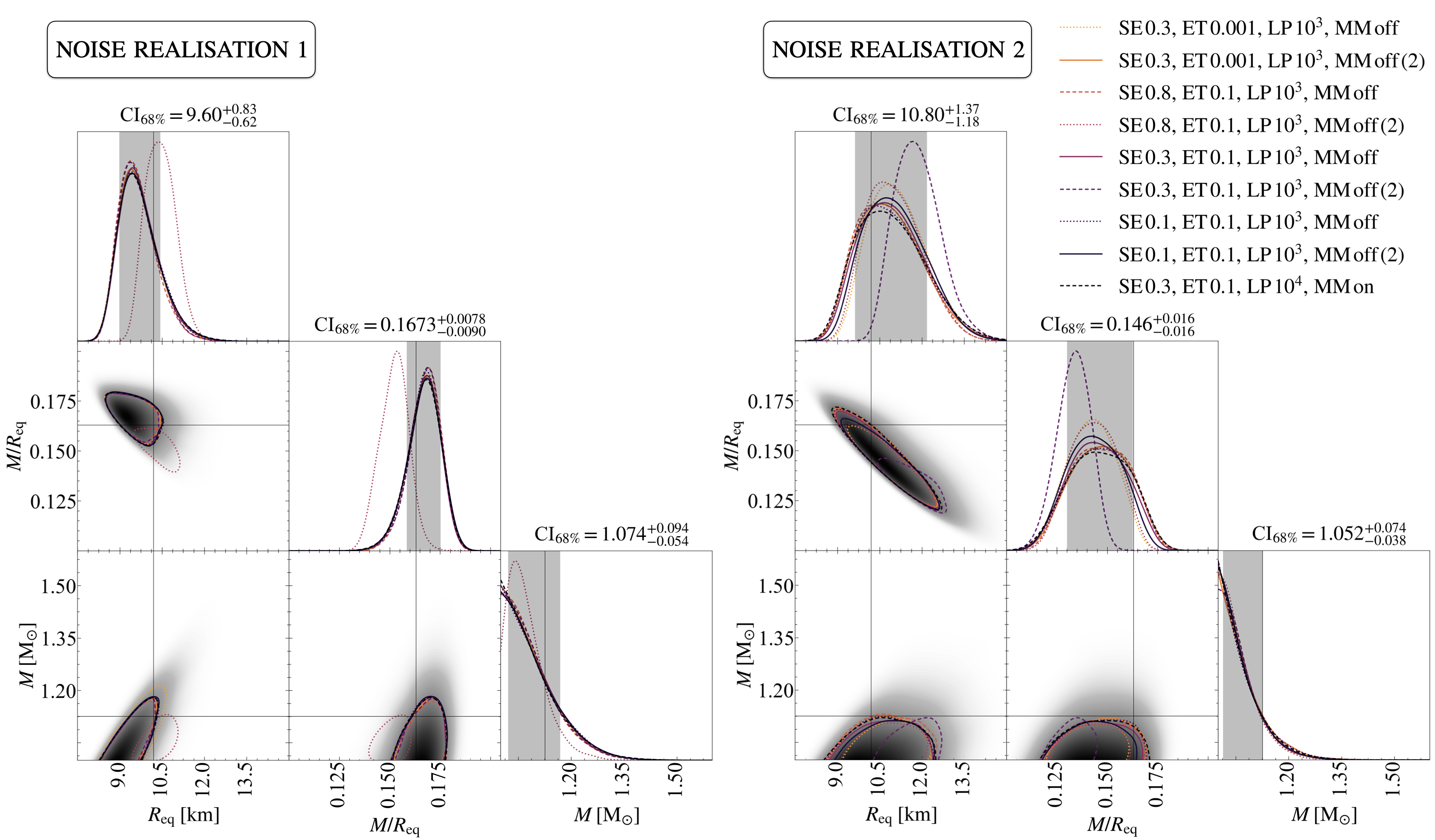
Figure 5: Posterior distributions (smoothed by GetDist KDEs) from 18 runs, for radius, compactness and mass. Results are obtained using data sets produced with two different noise realisations, labeled as one (left panel) and two (right panel). The two data sets were generated and analysed with the ST-U model. Each of the two plots shows posteriors from 9 inference runs which use different MultiNest settings, as reported in the legend (for definitions see Section 2.4). On top of the 1D posteriors, we report the 68% credible intervals (representing the area within the 16% and 84% quantiles in the 1D marginal posterior mass) starting from the median of the distributions. These values, as well as the colored areas, refer to the two runs enabling the mode-separation modality (dashed black lines). The lines in the 2D plots represent the 68% credible areas of the 2D marginalized posterior, while the shadow refers to the whole distributions of the inferences enabling the mode-separation modality. The thin solid black lines represent the injected values. Overall the various settings seem to recover consistent marginalised posteriors, while the different noise realisations adopted to build the two analysed data sets have a significant impact on the shapes of these distributions. The outlier within the runs in the left panel has MultiNest settings: SE 0.8, ET 0.1, LP $10^{3}$, MM off (2). The outlier within the runs in the right panel has MultiNest settings: SE 0.3, ET 0.1, LP $10^{3}$, MM off (2).

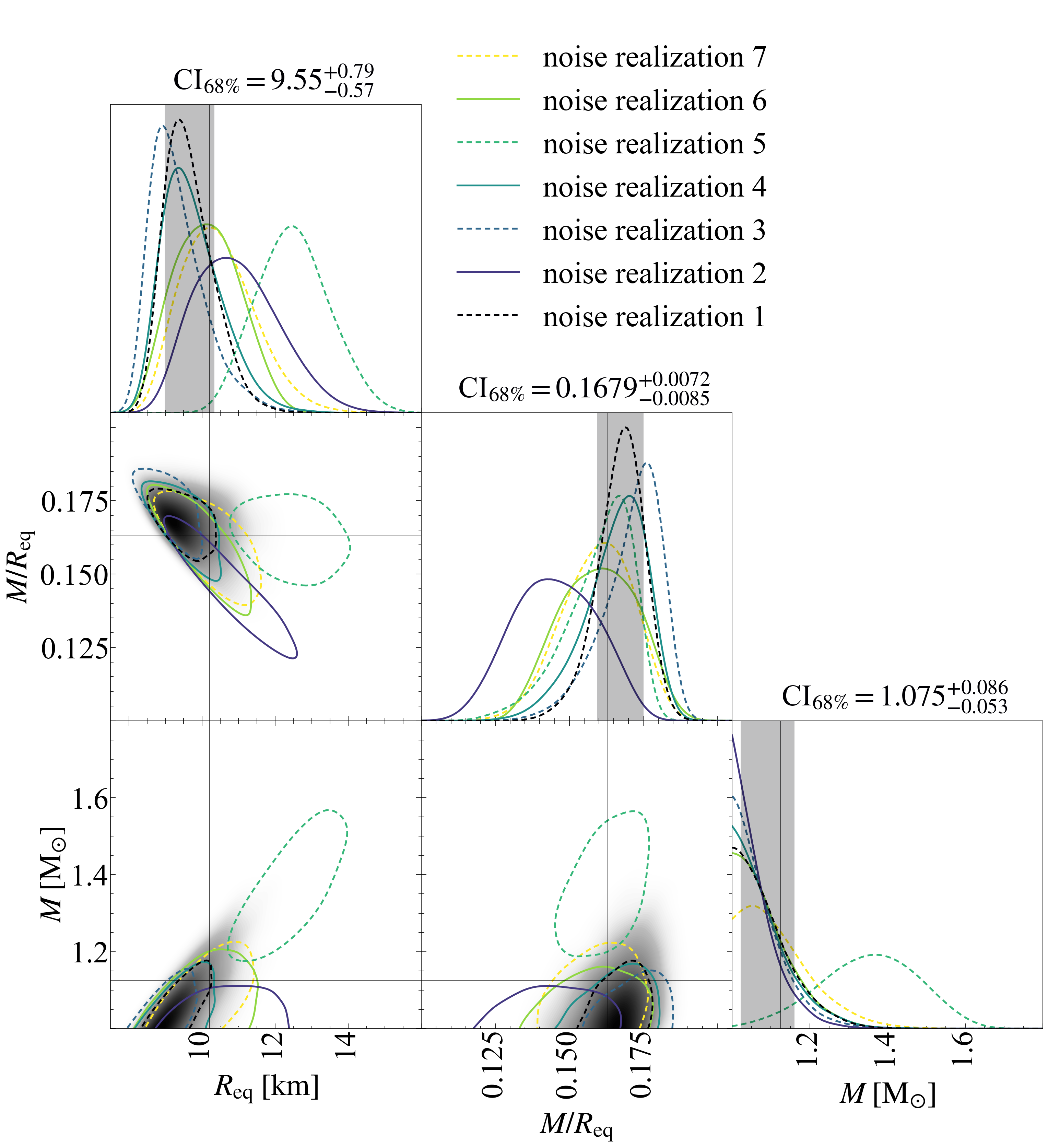
Figure 6: Posterior distributions (smoothed by GetDist KDEs) of radius, compactness and mass. Results are obtained using data sets produced with 7 different noise realisations, labeled from 1 to 7 in the legend. The data sets were generated and analysed with the ST-U model. Credible intervals and colored areas refer to the inference run labeled as noise realisation 1 (also represented with dashed black lines). See caption of Figure 5, for further details on the plot. These inference runs were performed with the X-PSI and MultiNest settings described in the Sections 3.3.1, 2.4 and reported in Table 2. As expected the different noise realisations introduce some scatter in the marginalised posteriors. The outlier (see especially the mass plot) is the run correspondent to noise realisation 5, the presence of this outlier may be simply due to random fluctuations arising in the sampling process (see indeed also the presence of outliers in Figure 5). The purple line delineating broad radius and compactness posteriors represents results from noise realisation 2.

	Mode 1	Mode 2	Mode 3
$\left<R_{\mathrm{eq}}\right>$ [km]	9.7,10.9(13.1)	9.9,13.4(14.6)	(15.3)
$\sigma_{R_{\mathrm{eq}}}$ [km]	0.7,1.2 (1.5)	1.3,1.7(1.0)	(0.5)
$\left<M\right>\,\mathrm{[M_{\odot}]}$	1.1,1.1(1.4)	1.1,1.2(1.5)	(1.6)
$\sigma_{M}\,\mathrm{[M_{\odot}]}$	0.1,0.1(0.2)	0.1,0.2(0.2)	(0.2)

Table 4: Means $\left<\cdot\right>$ and standard deviations $\sigma$ of the mass $M$ and equatorial radius $R_{\mathrm{eq}}$ posterior distributions. The different values correspond to the two (three) modes found by the X-PSI inference run when using the ST-U model to analyse a data set generated with the ST-U model -noise realisation 1, 2 and, in brackets, with the ST+PST-noise realisation 1.

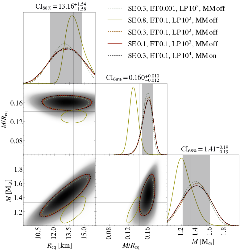
Figure 7: Posterior distributions (smoothed by GetDist KDEs) of radius, compactness and mass. The data set was generated adopting the ST+PST model (noise realisation label 1) and analysed assuming the ST-U model. Credible intervals and colored areas refer to the inference run enabling the mode-separation modality (also represented with dashed black lines). See caption of Figure 5, for further details on the plot. The inference runs shown in this plot were performed with the MultiNest settings reported in the legend (see Section 2.4 for definitions) and in Table 2. For all inferences, the injected parameter values are in the bulk of the marginalised posteriors even though the model adopted for inferences does not allow for the complex configuration used to generate the data set. The obtained distributions also well resemble the ones obtained when the correct model is used (see Figure 9). The outlier corresponds to the run with MultiNest settings: SE 0.8, ET 0.1, LP $10^{3}$, MM off and again it may simply be due to statistical fluctuations, possibly reflecting the need of more stringent sampling parameters.

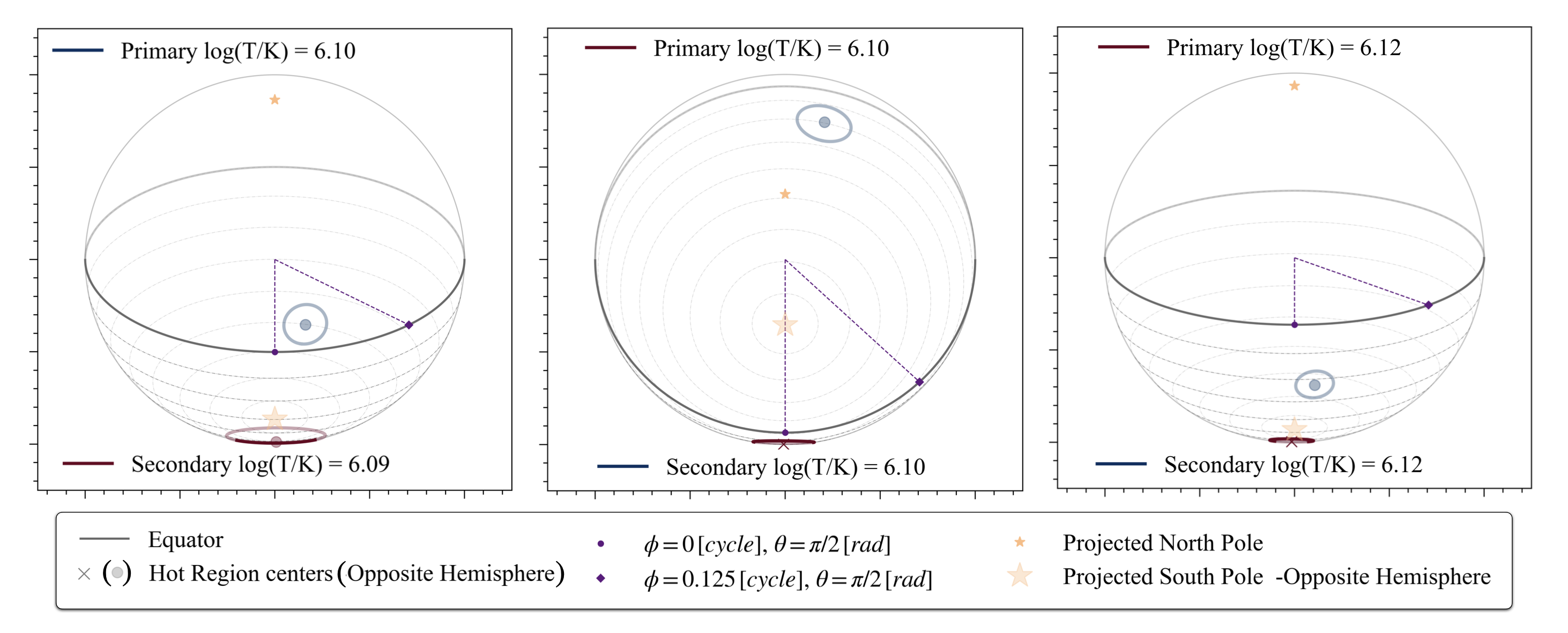
Figure 8: Schematic representation of the the hot spot configurations, as seen from Earth, for the three modes found by the X-PSI inference run when using the ST-U model to analyse a data set generated with ST+PST. The specific configurations correspond to the maximum likelihood sample associated with each mode (for other details, see the caption of Figure 3).

4.2 Inferences with the ST+PST Model

We present here the results obtained with inference runs adopting the ST+PST model, as reported in Table 3, particularly focusing on the analyses of data generated with the same ST+PST model (results obtained with mismatching models are reported in Section 4.3).

4.2.1 Noise and Settings

Figure 9 shows the impact of different noise realisations (left corner plot) and different MultiNest and X-PSI settings (right corner plot) on the inferred posteriors of mass, radius and compactness. Note that for the data set described by the noise realisation 1, we report results from a run with different MultiNest settings (LP $10^{4}$ and MM on) compared to the runs on the other two data sets (LP $6\times 10^{3}$ and MM off). In all the reported runs, the injected values lie within the 2D $\sim 95.4\%$ credible regions. Looking at the 1D posterior distributions, we find that, for similar analysis settings, the parameter recovery performance of X-PSI is worse for the more complex model ST+PST than for the simpler ST-U model. In particular, when broadening our attention to all the parameters describing the ST+PST model, the three runs reported in the left panel of Figure 9 recover within the 1D 68% credible interval: 7 ($\sim 43\%$, for the case of noise realisation 1), 5 ($\sim 31\%$, for the case of noise realisation 2) and 3 ($\sim 19\%$, for the case of noise realisation 3) parameters over the 16 describing the ST+PST model. These recovery rates are all below the expected range of $\sim(56-81)\%$ (calculated as 16% and 84% quantiles of a binomial distribution describing a sample of size $n=16$ and success rate $p=68\%$) and are mostly connected to geometrical parameters.

The variability due to noise looks comparable to the variability generated by different MultiNest settings. Among them, the number of live points seems to make the biggest difference, in terms of parameter recovery. If LP $\gtrsim 5\times 10^{3}$, the posterior distributions become wider and slightly shift toward the correct mass and compactness values. Figure 9 also demonstrates that, while noticeably reducing the required computational resources, using the X-PSI low resolution described in Section 3 only slightly modifies our posterior distributions compared to the X-PSI high resolution runs.

4.2.2 External Constraints, Degeneracies and Posterior Multi-Modal Structure

Effects of external Constraints. In Figure 11, we show the impact on mass, radius and compactness posteriors of different external constraints. Comparing it with the results in Figure 9, it is clear that adding constraints on mass and distance significantly reduced the widths of the radius posterior; however, including the constraints on the inclination, in our test case, biases our findings (we discuss these results in details in Section 5.3).

Degeneracies. The complexity of the ST+PST model introduces additional degeneracies between the parameters (see also Section 2.5 of R19, ); in particular, in view of our low sensitivity to the smaller details describing the hot spot shapes, many different parameter vectors are able to reproduce quite well the analysed data (see e.g., the small differences reported in Figure 12 and discussed in Section 5). This can be qualitatively understood, for example, looking at the top plots of panels A and C, reported in Figure 12. They represent the hot spot configurations found in our inference runs on data generated with the ST+PST model. In particular the top plots of panels A and C represent the maximum likelihood sample of the runs analysing data simulated with noise realisations 1 and 3 (the results for noise realisation 2 mimic the configurations of panel A). Although both of these represented configurations can well replicate the simulated data, only the latter recovers a hot spot configuration that resembles the correct one (right panel of Figure 3). This is probably due to the weak sensitivity of our analysis to e.g., the direction of the thermally emitting arc (which indeed faces the right direction in panel C and the wrong one in panel A). The additional degeneracies introduced by the complexity of the model therefore compromise the recovery of the model parameters (as demonstrated by the low rate of recovered parameters mentioned in Section 4.2.1), which set the geometry of the emitting NS surface.

Posterior Multi-Modal Structure. When applied to the data set generated using the ST+PST model, our inference runs employing mode-separation modality find two different modes with comparable maximum likelihood values. The configuration corresponding to the maximum likelihood samples of these two modes are shown in the top plots of panels A and B, Figure 12. While the main mode approximately recalls the simulated configuration of the hot spots, the secondary mode resembles the ST-U configuration in Figure 3. With the averages and standard deviations reported in Table 5, the recovered radius and mass corresponding to this secondary mode are, however, quite close to the injected values.

	Mode 1	Mode 2
$\left<R_{\mathrm{eq}}\right>$ [km]	13.8(9.7)	13.4(9.7)
$\sigma_{R_{\mathrm{eq}}}$ [km]	1.3(0.6)	1.2(0.7)
$\left<M\right>\,\mathrm{[M_{\odot}]}$	1.4(1.1)	1.4(1.1)
$\sigma_{M}\,\mathrm{[M_{\odot}]}$	0.2(0.1)	0.2(0.1)

Table 5: Means $\left<\cdot\right>$ and standard deviations $\sigma$ of mass $M$ and equatorial radius $R_{\mathrm{eq}}$ posterior distributions. The different values correspond to the two modes found by the X-PSI inference run when using the ST+PST model to analyse a data set generated with the ST+PST model -noise realisation 1 and, in brackets, with ST-U-noise realisation 1.

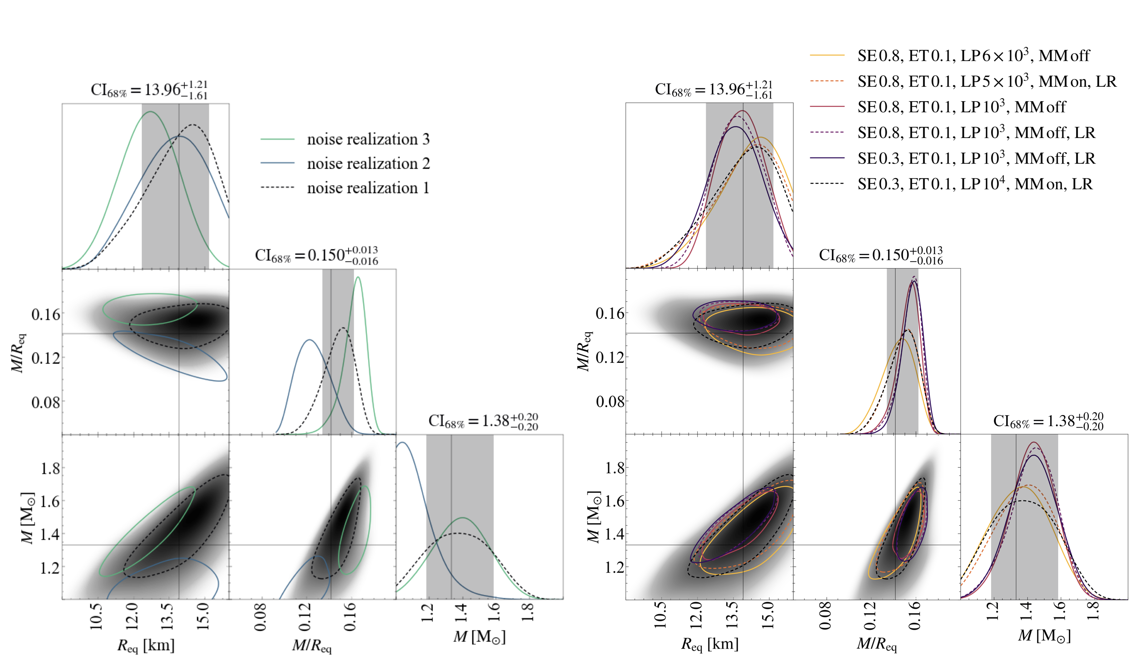
Figure 9: Posterior distributions (smoothed by GetDist KDEs) of radius, compactness and mass. The data sets were generated and analysed adopting the ST+PST model. In the left panel, we present results obtained using data sets produced with three different noise realisations, labeled from one to three in the legend. For all these runs we adopted the X-PSI low resolution setting (LR), SE 0.3 and ET 0.1. For noise realisation 2 and 3, we use LP $6\times 10^{3}$ and MM off, for noise realisation 1 LP $10^{4}$ and MM on (the right panel demonstrates that these two settings lead to similar results). This plot shows that, given these settings, model and observing properties, our recovered posterior distribution is sensitive to the noise realisation adopted to generate the analysed data sets. In the right panel, we show the corner plots corresponding to different runs analysing the data set generated with noise realisation 1 and different X-PSI and MultiNest settings as shown in the legend. The three curves with broader posteriors represent the runs with $\geq 5\times 10^{3}$ LP (the first two and the last one in the legend). This corner plot demonstrates the need of a large number of live points to sensibly estimate the width of the marginalised posteriors. All these inference runs are described in Sections 3.3.2, 2.4 and their details are reported in Table 3. In both plots credible intervals and colored areas refer to the inference run adopting SE 0.3, ET 0.1, LP $10^{4}$, MM on and LR as MultiNest and X-PSI settings (represented with dashed black lines), and applied to the data set generated with noise realisation 1. See caption of Figure 5, for further details.

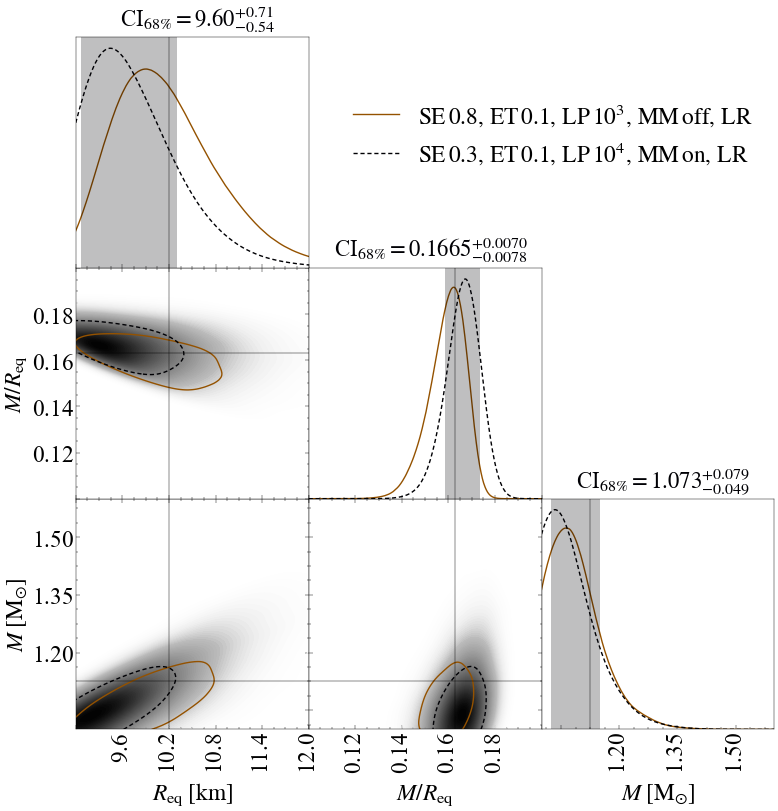
Figure 10: Posterior distributions (smoothed by GetDist KDEs) of radius, compactness and mass. We present results from two ST+PST inference runs analysing the data set generated with the ST-U model defined by noise realisation 1; MultiNest settings are reported in the legend. LR stands for the X-PSI low resolution setting. Credible intervals and colored areas refer to the mode-separation inference run (also represented with dashed black lines). The injected parameter values are well within the bulk of the obtained marginalised posteriors. These distributions are also similar to ones found when the ST-U model was used to analyse this data set. Increasing the number of live points used in the sampling procedure to $10^{4}$ slightly shifts the obtained posterior distributions, highlighting that $10^{3}$ live points are probably not enough to adequately explore the parameter space. See caption of Figure 5, for further details.

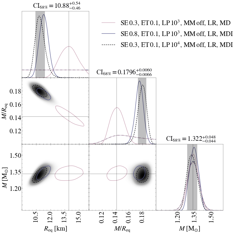
Figure 11: Posterior distributions (smoothed by GetDist KDEs) of radius, compactness and mass. We report posterior distributions for data analysed and generated with the ST+PST model. With these inference analyses we explore the effect of external constraints on our analysis (see Section 3.3.2 for more details). MultiNest and X-PSI settings, as well as the model parameters a priori constrained (M stands for mass, D for distance and I for inclination), are shown in the legend. For this plot we used the data generated with noise realisation 1. Credible intervals and colored areas refer to the inference run obtained with constraints on mass, distance and inclination and using $10^{4}$ live points (also represented with dashed black lines). For clarity, here we also show the 1D marginalised prior distributions on radius, mass and compactness with dash-dot lines. Including the inclination constraints (which is otherwise not well recovered) shifts the inferred marginalised posterior distributions away from the injected values of radius and compactness, highlighting the multi-modal structure and complexity of our posterior surfaces. See caption of Figure 5, for further details.

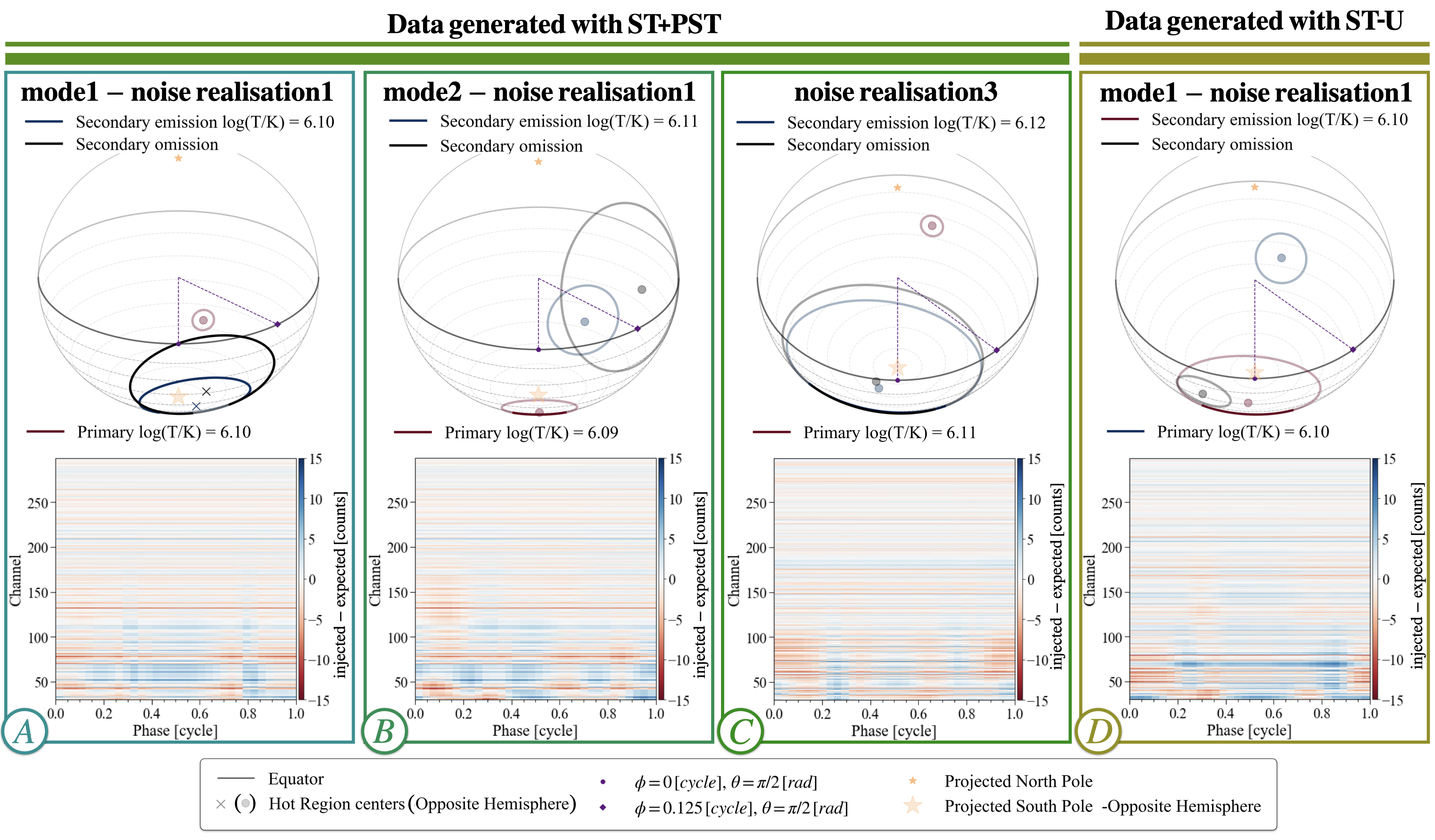
Figure 12: Results for three different ST+PST runs: panels A and B refer to the SE 0.3, ET 0.1, LP $10^{4}$, MM on, LR run on data generated with the ST+PST model and noise realisation 1; panel C to the SE 0.3, ET 0.1, LP $6\times 10^{3}$, MM on, LR run on data generated with the ST+PST model and noise realisation 3; and panel D to the SE 0.3, ET 0.1, LP $10^{4}$, MM on, LR run on data generated with the ST-U model and noise realisation 1. Mode numbers are specified only for analyses employing the mode-separation modality (also referred to as mode-separation variant). Panel B corresponds to the maximum likelihood sample belonging to the secondary mode; all other panels refer to the maximum likelihood sample of their respective inference runs. Top panels: schematic representation of the the hot spot configurations, as seen from Earth. Bottom panels: difference in counts between the injected data and the expected counts correspondent to the considered sample of their respective runs (as a reference, in the injected data the maximum count per phase bin and channel is $\sim 700$). The small differences in counts, always smaller then $\sim$ twice the Poisson noise standard deviation, imply that significantly different configurations and parameter values can arise from very similar data sets, assuming the current properties of the PSR J0030$+$0451 NICER observations.

Data/Analysis	ST-U	ST+PST
ST-U	$-35657.1\pm 0.1$	$-35655.5\pm 0.1$
ST+PST	$-35740.5\pm 0.1$	$-35736.2\pm 0.1$

Table 6: Natural logarithm of evidences and their errors (as reported by MultiNest) for inference runs with settings SE 0.3, ET 0.1, LP $10^{4}$, MM on. X-PSI low resolution is applied for all inference runs assuming the ST+PST model. Different rows signify different models used to generate the analysed data; different columns correspond to different models adopted in the inference runs.

	Mode 1	Mode 2
$\mathbf{max(\mathcal{L})}$	$1.14\,M_{\odot}\,(10.9\,\mathrm{km})$	$1.01\,M_{\odot}\,(8.9\,\mathrm{km})$
$\mathbf{max(\mathcal{P})}$	$1.09\,M_{\odot}\,(9.0\,\mathrm{km})$	$1.02\,M_{\odot}\,(10.1\,\mathrm{km})$
$\mathbf{mean}$	$1.12\,M_{\odot}\,(9.9\,\mathrm{km})$	$1.09\,M_{\odot}\,(9.7\,\mathrm{km})$

Table 7: Mass and radius values (in brackets) of the maximum likelihood ${max(\mathcal{L})}$, maximum posterior ${max(\mathcal{P})}$ and the mean of the marginalised 1D posterior distributions for the SE 0.3, ET 0.1, LP $10^{4}$, MM on inference run, employing the ST-U model on a data set generated with the same model and noise realisation 1.

4.3 Model Mismatches

4.3.1 ST-U inferences on data produced with the ST+PST model.

In Figure 7 we show 1D and 2D posterior distributions of mass, radius and compactness for ST-U runs on data produced with the ST+PST model. This figure suggests that X-PSI inference runs can recover these parameters even when the model used for inference does not capture the full complexity of the ground truth. However, in view of the previous findings concerning our sensitivity to noise realisations, our results cannot be easily generalised, i.e., this could be restricted to a subset of parameter values and noise combinations. To generalise our findings we would need to consider a statistically significant number of model parameter vectors and noise realisations. For this data set we also perform an inference run enabling the mode-separation modality. We find three modes from this analysis; the configurations corresponding to their respective maximum likelihood samples are reported in Figure 8. The corresponding means and standard deviations for mass and radius are reported in brackets in Table 4. In this case, the main mode is also clearly dominant in terms of likelihood and evidence calculation, while the other two modes show comparable maximum log-likelihood and local evidences.

So far for X-PSI analyses, we have mostly relied on residuals to verify how well our solution can represent the data. In the context of X-PSI, residuals are defined, per bin in channel and phase, as the difference between the data and the inferred expected counts divided by the square root of the same expected counts (see e.g. bottom panel of Riley et al., 2019). Interestingly, although the ST-U model can not represent a configuration complex as the one injected to simulate the data (shown in the right panel of Figure 3), the residuals do not present any anomalous feature and therefore look compatible with Poisson noise.

4.3.2 ST+PST inferences on data produced with the ST-U model.

In Figure 10, we report posterior distributions for the mass, radius and compactness obtained when analysing data produced with the ST-U model, assuming the more complex ST+PST model. The ST+PST model allows configurations that can well approximate the ST-U ones (ST-U is nested in ST+PST). The model can therefore identify, as a main solution, samples that well represent the correct and injected parameter vector. Also in this case mass, radius and compactness are well recovered by our analysis. In particular, both inference runs on ST-U generated data return 1D/2D posterior distributions whose 68% credible intervals/regions include the injected values of these parameters. However, also here, the various dependencies of our findings and the restricted test cases prevent us from generalising this conclusion.

As for the runs in the right panel of Figure 5, also here the more computationally expensive MultiNest settings (LP $10^{4}$, MM on) lead to slightly wider and more accurate posteriors compared to the other runs. However, now the complexity of the model, and the degeneracies between its parameters, yield two different modes in the posterior, with similar mass and radius (both correctly recovered) and comparable in maximum likelihood and local evidences. The corresponding hot spot configurations of the two modes are however significantly different from one another. To understand this difference, we can compare the top plots of panels B and D, Figure 12. The configuration corresponding to the maximum likelihood sample of the main mode is indeed represented in the top plot of panel D, Figure 12. The (exact) configuration correspondent to the secondary mode is not reported here, but it is qualitatively equivalent to the secondary mode found analysing data generated with the ST+PST model and shown in the top plot of panel B, Figure 12.

Similarly to the previous case, also here the mismatch between the model adopted to create the data set and the one used to analyse it never appears as a clear feature in the residuals. This is, in this case, less surprising, since the model used for inference is the most complex between the two.

5 Discussion

Here we discuss the results presented in Section 4. For the (albeit limited) cases considered in this paper, our inference runs on simulated data illustrate the adequacy of X-PSI analysis in recovering mass, radius and compactness given PSR J0030$+$0451-like NICER data. This reinforces and expands the findings reported in Riley (2019); Bogdanov et al. (2021), which also included ST-U recovery tests. In particular, compactness, mass and radius are recovered within the 95.4% 1D credible interval (when no additional constraints are applied on the inclination) for all of the tested data sets, except the one generated with the ST-U model and noise realisation 5. In the following we reflect on the meaning of our findings, particularly focusing on the role of different analysis conditions, and discuss the few anomalous encountered cases and the caveats of our analysis.

The ST+PST inference runs for which we adopted mock constraints on mass, distance and inclination are separated out and discussed in Section 5.3.

5.1 The Effect of Noise, Analysis Settings and Randomness in the Sampling Process

This study shows a clear dependence of our results, including our sensitivity to MultiNest settings, on the noise realisation. This is shown for the ST-U model in Figures 5 and 6, and in Figure 9 for the more complex ST+PST model. This implies that each data set will require its own study to assess the robustness of the results. In Figure 5 we see indeed that the posterior distributions for the data set created with ST-U and noise realisation 1 (left corner plot) are much more similar to each other than the ones obtained analysing the data set created with noise realisation 2 (right corner plot). Note that the posterior distributions in the left corner plot are so insensitive to the different tested MultiNest settings, that even increasing the number of live points by about an order of magnitude does not seem to make any significant difference (despite expectations, see for example Ashton et al., 2019; Riley et al., 2021). However, for both of the ST-U data sets analysed with different MultiNest settings (i.e. the data generated with noise realisation 1 and 2), 1 of our 9 inference runs shows a different behavior. This is also the case for the ST-U parameter estimation runs for the data set created with the ST+PST model (yellow curve in Figure 7). Given our limited tests, it is not possible to conclusively assess the main origin of such fluctuations. They clearly have a stochastic component, since, for noise realisations 1 and 2, they appear in only one of two identical analyses; however, it is unclear whether they could be exacerbated by poorer MultiNest settings, e.g., by fixing SE to 0.8 (two out of the three outliers have this setting). The poor statistics also prevent a significant evaluation of the role played by the noise realisation on the rate of occurrence of these anomalous results.

Despite the noise fluctuations, compactness is recovered within the $\sim 68\%$ credible interval for almost all cases. Exceptions are: the inference run on a data set built with the ST-U model and noise realisation 2 (where the injection value lies just outside it, see right panel of Figure 5) and the inference run on the data set built with the ST+PST model and noise realisation 3 (which qualitatively recovers the injected hot spot geometry). These results are consistent with expectations, although quantitative expectations can only be formulated assuming independence between the parameters. Mass and radius are also well recovered by our analyses: we recover mass within the $\sim 68\%$ credible interval for 7 of the 10, ST-U and ST+PST, data sets and the radius for 6 of them. These rates both fall within the approximate expected 5-8 range, estimated as explained in Section 4.1.1. The main deviation comes from data generated with ST-U model and noise realisation 5. This could either be due directly to the noise realisation, such that repeated inference runs (with the default or better MultiNest settings) would show the same behaviour, or it could just be due to a random fluctuation (as we see happening for 1 of the 9 ST-U inferences runs on data characterised by noise realisation 1 and 2). We have indeed just argued that the MultiNest settings required to adequately explore the parameter space may vary for different noise realisations. An inspection of this simulated data set does not reveal any particular anomalous feature; we can only identify a slightly lower rate of high counts for channels $\sim(30-60)$ and phases $\sim(0.2-0.6)$ compared to the other noise realisation. Given the computational resources available to us for this study, we currently cannot fully determine the statistical relevance of this deviation nor its origin. Its relatively low rate, however, is in principle consistent with statistical fluctuations and is therefore not particularly worrying.

As shown in Figure 6, different noise realisations can yield very different sizes of the mass, radius and compactness credible regions. This finding seems also completely independent from the model adopted to infer the parameter values (see the similarities between the left plot of Figure 5 and Figure 10). Our results therefore highlight the crucial role played by stochastic processes on the recovered mass and radius uncertainties and reveal scatter that could complicate and affect their predictions.

5.2 Model Complexity

Both ST-U and ST+PST models are able to mimic the data of PSR J0030$+$0451 collected by NICER (see e.g., Figure 1 in R19, ). Without accounting for noise realisations, the data sets produced, assuming these models and their correspondent parameter vectors as reported in Table 1, are not only similar in overall counts but also in the hot spot and background contributions to the data. This can be seen in Figure 13, comparing e.g., the mostly overlapping dashed gray and solid black lines, which represent the background counts used (and found in preliminary analyses of the revised PSR J0030$+$0451 NICER data set ) to simulate data with the ST-U and the ST+PST model respectively. These strong similarities show that, even for the same background, there are significant degeneracies in the model and parameter space able to explain PSR J0030$+$0451-like data. When we use the ST-U model on data produced with the ST+PST model, we find a configuration which very much resembles the one used for generating ST-U data sets and reported in the left panel of Figure 3. In particular, independently from the model used to create the analysed data set, the ST-U inference run enabling the mode-separation modality finds similar hot spot configurations for the primary and secondary modes. When analysing the data set created with the ST+PST model, however, a tertiary mode is also revealed (the geometries of all modes are shown in Figure 8).

The ST+PST inference runs show slightly different behaviour: the primary mode found when analysing the data generated with the ST-U model shows a configuration in between the ST-U and the ST+PST one (panel D of Figure 12). Indeed temperatures, inclination and hot spot locations resemble the configuration injected for the ST+PST model, while hot spot sizes and resulting geometries recall the ST-U injection. Therefore, although the ST-U injected configuration could be very well approximated within the ST+PST model, the larger available parameter space guided the inference process to a geometry which differs from it. For two of the three data sets generated with the ST+PST model, we also find a configuration which slightly differ from the injected one. Our findings therefore seem to suggest that the complexity introduced by the ST+PST model makes it harder for the sampler to identify the correct parameter values. On the other hand, mass, radius and compactness are always well recovered (see Tables 7 and 5); in particular we see that the posterior shapes of these parameters seem to be independent of the model adopted for the analysis. This is surprisingly different compared to the situation found in R19, where the mass and radius changed considerably depending on the model adopted for the X-PSI analysis. Differently from the results of R19 (where the difference in log-evidence between the ST-U and the ST+PST models was of $\sim 10$ units), are also the values of the various evidences. From Table 6 we notice that there is never a decisive preference for one model compared to the other, since, given a data set, the evidences differ by just a few units in $\log$. Different behaviours compared to the data suggest that our simulations do not capture all features present in the data. At this moment, however we cannot conclusively assess if these discrepancies are strictly related to the specific noise realisations (see Section 5.1), limited to the two considered parameter vectors, or signs of some more profound differences (e.g., some aspect of the physics that is not being modeled).

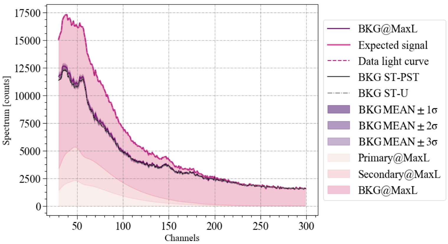
Figure 13: Background figure for the ST+PST inference run SE 0.3, ET 0.1, LP $10^{4}$, MM on, LR on data created with the same model and noise realisation 1. In shades of pink, from the lightest to the darkest we highlight the contribution to the data in counts per channel of the primary hot spot, the secondary hot spot and the background. The solid pink and dashed fuchsia lines represent respectively the total counts per channel expected according to our model and found in the data. With the solid purple line we show the background correspondent to the maximum likelihood sample of the inference run. From the strongest to the dimmest purple regions we show the $\pm 1$, $\pm 2$ and $\pm 3$ standard deviation regions. The solid black and the dashed gray lines (mostly overlapping) show the background added to the hot spot contribution to obtain the simulated data with the ST+PST and ST-U models respectively.

5.2.1 Degeneracies and Multi-Modal Structure in the Posterior and Likelihood Surfaces

A general discussion of degeneracies between model parameters is found in Sections 2.5.4 and 2.5.6 of R19; here we comment on them in relation to the specific findings of this paper. In the context of mock PSR J0030$+$0451 NICER data, our inference runs demonstrate the degeneracies between model parameters via the presence of a multi-modal structure in the posterior surface.

In this work we took advantage of the mode-separation modality offered by MultiNest. This has highlighted the presence of a multi-modal structure in the posterior surface, which does not comes as a surprise given the different configurations found in the nested models explored for PSR J0030$+$0451 NICER data in R19. As we comment below, naturally the extent to which degeneracies populate the parameter space is correlated with the degree of multi-modality present in the posterior surface. This should be kept in mind when comparing evidences between models; indeed higher evidences could arise from the introduction of a more adequate model to describe the data (i.e. for the presence of higher likelihood points) as well as from larger portions of the parameter space rendering similarly good solutions to represent the data.

For the ST-U inference runs, the difference in likelihood and evidence between the various modes is large enough to strongly prefer the correct mode; the performance of X-PSI in recovering injected parameters mimicking the secondary mode, has however not been checked. Although the mass and radius of the primary mode are always in reasonable agreement with the injected values, Table 7 shows that the radius values associated with the secondary mode change considerably depending on the specific considered data set (and therefore noise realisation). This variability may be due to an inadequate number of live points covering the specific mode, or due to random fluctuations.

Looking instead at the ST+PST inference runs we find a different situation. As mentioned above, in two of the three analysed data sets, we are unable to find the injected geometry (see Figure 12), even though all runs and both of the flagged modes display mass and radius posteriors compatible with the injected values (see Table 5 and Figure 9). Indeed multiple hot spot configurations can give rise to very similar PSR J0030$+$0451-like data sets. For all three runs in the left panel of Figure 9, the injected configuration had a likelihood difference from the maximum likelihood solution of only a few units in $\log$. This can also be understood e.g., by looking at the bottom plots of Figure 12. These plots represent the difference in counts, per energy channel and phase bin, between the injected data sets and the expected one, given by the maximum likelihood sample of that specific run or mode (corresponding to the hot spot geometry represented on the above panel). Note that the largest differences occur where the typical counts per energy channel and phase bin are a few hundred, so that the relative difference is never more than a few % ($\lesssim 10\%$). Given the number of counts characterising these bins, this percentage is always smaller than $\sim$ twice the Poisson noise standard deviation. This means that, assuming the same properties of the revised PSR J0030$+$0451 NICER data set (for more details see Vinciguerra et al., 2023, submitted), we expect no significant difference between the data produced with the various configurations (whose geometry is represented on the corresponding top panel).

If we integrate these plots over phase bins $i$ and energy channels $j$, we can define the variable

$$\mathfrak{D}=\frac{\sum_{i}\sum_{j}|d_{i,j}-c_{i,j}|}{\sum_{i}\sum_{j}d_{i,j}}\,,$$

where $c$ and $d$ represent numbers of counts respectively for inferred sample solutions and the injected data. For all the 4 cases (from panel A to D) presented in Figure 12, we find that the integrated difference $\mathfrak{D}$ between the injected data $d$ and the expected counts predicted by the run or mode $c$ (assuming its maximum likelihood sample) is smaller than the difference between the simulated data in presence and absence of noise $\mathfrak{D_{sim}}\sim 0.056$. This highlights the presence of some major degeneracies between our model parameters, as introduced in Section 2.3, for a PSR J0030$+$0451-like data set. We can use the top panels of Figure 12 to motivate some of them. The similar values of likelihoods and evidences between all of these configurations tells us that, with these simulated data sets, we are not very sensitive to the details of the shapes of either hot spot. For example the top plots of panels A and C show the arc of the PST region oriented in opposite directions, and in both cases a visual inspection of the residuals does not highlight any anomaly. Similar pulses can therefore be generated even when the parameters describing the hot spot significantly differ (e.g., a difference in the arc direction is rendered with the centre coordinates of the spherical caps having considerably different values). Similarly the emission from the ST hot spot seems to be captured by both a circular hot spot as well as an arc, comparing the top plots of panels A and B. Moreover we find that, in general, the most likely configurations presented in this paper cluster around values of inclinations between $i\sim 40^{\circ}$ and $i\sim 60^{\circ}$; the limits of this range also roughly correspond to the inclinations used to simulate data respectively with the ST+PST and the ST-U model. Focusing on the ST+PST inference results, Figure 12 shows that both inclination values can be recovered, independently from the model used to generate the analysed data. To generate data comparable to the analysed one, the hot spot geometry needs to adapt to the different inclination values. When we have lower inclination values, the hot spot, closer to the equator, needs to have lower colatitude to still be visible to an observer. Similarly the emitting region located closer to the South Pole needs to reach lower colatitude and cover a larger area to still be detectable in the correct phase interval.

The noise shifts the peak of the likelihood away from the true parameter values (as expected) and the sampler does not always identify modes of comparable likelihood.

The ST+PST analyses, for the data sets labeled with noise realisation 1 and 2, were unable to identify the likelihood peak corresponding to the true hot spot configuration, despite them having comparable likelihood values to the best fitting samples found. The absence of configurations similar to the injected one in the posteriors, despite the comparable likelihood value, reveal the inadequacy of the X-PSI and/or MultiNest settings adopted in our analyses for these specific cases. Indeed comprehensive tests, assessing the robustness of the obtained results and the level of coverage of the parameter space for ST+PST inference runs, are computationally demanding and we therefore decided to prioritise preserving compute time to carry out these kind of studies for the analysis of the upcoming and future new data sets.

The inference run on data with noise realisation 3 (the one which recovered the injected geometry) instead collected samples also resembling the configuration found as the main mode for the other two noise realisations. Despite the difference of only a few units in $\log$ likelihood, however, this latter configuration was not prominent enough to form a clear feature in the posteriors.

Importantly none of the solutions found, including the ones pointing to a slightly different geometry compared to the true ones, exhibit any anomaly in the residuals. Once we are assured that the parameter space has been exhaustively explored and if multiple solutions are revealed, it is possible to evaluate them considering a broader context, including e.g., radii inferences from other NICER sources, constraints/indications coming from independent phenomena, such as gravitational waves (see e.g., Raaijmakers et al., 2021), or even from theoretical advancements. Alternatively, this independent information could also be incorporated in follow up test runs with the application of tighter priors on the radius.

5.3 External Constraints

The impact of the multiple modes arising from the posterior surface could be, at least in principle, mitigated by external constraints, e.g., on mass, distance and inclination (coming from radio observations) or on the background spectrum. Applying such constraints can also considerably reduce the uncertainties on the inferred parameters, including radius. This is clearly visible comparing the sizes of the posteriors in Figure 11 to the ones in Figure 9.

In the cases analysed in this paper, however, tight constraints on inclination end up biasing our results, even affecting the radius inferences, which were otherwise correctly estimated. In addition, these biased solutions do not exhibit any anomaly in the residuals. Comparing the two ST+PST runs with constrained inclination prior, we notice that increasing the MultiNest resolution settings (in particular increasing the live points and lowering the sampling efficiency) improves the performances of our analysis. In particular it increases the likelihood of the maximum likelihood sample by a factor of $\sim 15$ in $\log$. The reason becomes apparent when inspecting the posterior distributions of the SE 0.3, ET 0.1, LP $10^{4}$, MM off run. Here we find a clear bi-modality: this inference run is able to correctly identify the more complex hot spot, however it also shows the presence of an additional secondary mode where the PST region is actually identified as an ST hot spot and vice-versa. This local maxima in the posterior surface seems to dominate the progression of the less computationally expensive run, which is therefore unable to reveal the additional, higher-likelihood mode.

However, neither our runs is able to identify the mode associated with the correct solution. By checking the likelihood value correspondent to the injected parameter vector, we notice that in both cases the log-likelihood of the injected solution is greater than the maximum likelihood solution found by the sampler; however only by a factor of a few in $\log$, for the SE 0.3, ET 0.1, LP $10^{4}$, MM off run. This suggests that another mode is present in the posterior surface and that the relevant part of the parameter space has not yet been adequately explored and/or that the prior volume supporting the mode, found without external constraints, has now been significantly reduced, such that it is harder to identify it. Indeed neither inference run found samples space close to the injected vector.

Although our work here has revealed that systematics can occur in the PPM analysis of NICER data, it also highlights that these can be mitigated by convergence tests, proving that the parameter space has been exhaustively explored. These should include increasingly more computationally expensive runs, with more and more stringent sampling requirements, as well as repeated inferences, assessing the variability due to the random processes, and posterior predictive distribution tests. Since we find that in general mass and radius are well recovered if no further constraints are added (even when the geometry parameters are not), our findings also suggest it may be beneficial to accompany inference runs with tight constraints on geometry parameters, when these are available, with runs that do not consider them. We are now prioritizing computer resources to ensure that we can carry out such targeted and comprehensive convergence tests on upcoming real data sets.

In the two ST+PST inference runs (with tight constraints on the inclination prior) here considered, applying background constraints would have not improved our findings, since the recovered background is always very similar to the injected one (see Figure 13). This, however, is not necessarily the case for the real data. On the contrary, if the background constraints could cut the level of background found with these analyses, it would eliminate a large group of possible - and possibly similarly good - solutions, maybe uncovering a prominent but less ambiguous portion of the parameter space. NICER background constraints have been applied on NICER data sets for PSR J0740$+$6620 (Salmi et al., 2022) and are currently being adopted for NICER analyses on new, and expanded NICER data sets for multiple NICER sources.

Similar constraints could also be provided through observations of NICER sources by other X-ray (and in particular, imaging) telescopes. For example in Riley et al. (2021); Miller et al. (2021), the portion of the NICER data attributed to the thermal emission of PSR J0740$+$6620, was constrained by the XMM-Newton observations. Since coherently including XMM-Newton data into X-PSI inference has been proven very beneficial, this procedure is also planned for other NICER sources.

5.4 Implications for PSR J0030+0451

Our study demonstrates that the analysis (X-PSI and MultiNest) settings need to be tailored to each specific data set and applied assumptions. In particular our work places some of the findings, reported in R19, in a broader context. The new uncertainties and complications of the analysis process revealed in this study imply that PSR J0030$+$0451 NICER results and their interpretation need further investigations. Such studies are crucial to validate the robustness of the implications on the equation of state and the magnetic field structures derived from previous PSR J0030$+$0451 NICER works. This is the main target of the upcoming reanalysis of NICER data (Vinciguerra et al., 2023, submitted).

5.5 Implications for PSR J0740+6620

PSR J0740$+$6620 is the second NICER source, whose PPM analyses have been publicly released by the NICER collaboration. The inference of PSR J0740$+$6620’s radius has crucial implications for the equation of state, given the very high mass, independently inferred from radio observations of $2.08\pm 0.07\,M_{\odot}$ (Fonseca et al., 2021). The same study has also provided meaningful constraints on distance and inclination. This information has been used in the X-PSI analyses of PSR J0740$+$6620 NICER data sets (Riley et al., 2021; Salmi et al., 2022). While no simulation has yet been published to test the recovery performance of X-PSI for similar parameter vectors, we expect these studies to have delivered accurate results (T. Salmi et al. 2023, in preparation). In Riley et al. (2021), PSR J0740$+$6620 was analysed with very different numbers of MultiNest live points, proving stability in the solution found and the absence of other high-likelihood modes (a high number of live points, $4\times 10^{4}$, was in the end used for production runs to correctly render the width of the posteriors; however no significant shift was found compared to runs with fewer live points). This more detailed analysis was possible for PSR J0740$+$6620, and not for PSR J0030$+$0451, because of its fewer counts, lower signal to noise ratio and the simpler model (the ST-U model was indeed identified as the headline model).

5.6 Caveats

The simulations presented in this paper are far more exhaustive, and hence computationally expensive, than those done previously, but are still finite in scope. From them we have learned that the noise greatly impacts our results, changing, in particular, the width of our posteriors as well as their sensitivity to the analysis settings. The extent of this effect however could not be fully inferred with our limited resources.

Our findings could also be significantly affected by the particular choices of parameter vectors and background spectra adopted to simulate the considered data sets. Our sensitivity to such choices has not been tested here; however the difference in behaviour found in this paper, compared to the results reported in R19 (e.g., in the effect of using different models on radius inference and evidence), suggests their impact could be significant. This difference in behaviour could also lie only in the parameter vector used for the ST+PST model. This parameter vector was indeed found in a low-resolution inference run (Vinciguerra et al., 2023); while data were then built with it at higher resolution. This change might have produced some features in the simulated data sets which have no correspondence in the real data and may therefore explain the difference behaviour (in particular for the evidence comparison with different models) between simulated and real data (see evidence discussion in Section 3 of R19, ). Indeed when simulating the ST+PST data, the inferred exposure time differs from the real one by $\sim 50\,$s, in contrast with only $0.01\,$s in the case of the ST-U model and parameter vector.

We also highlight here that in all the tests presented in this work, the physics used to produce the synthetic data sets was known and mostly (except for the ST-U inference runs on data produced with the ST+PST model) entirely captured by the inference set-up. This is not necessarily the case for the analysis of real data obtained by NICER, where the physics is sometimes assumed (e.g., for the atmosphere composition) and sometimes approximated (e.g., for the specific hot spot shapes).

5.6.1 Correlations

To correctly interpret our results, we need to be aware of the various correlations between the parameter models. For example, when we presented the percentage of parameters recovered within the $\sim 68\%$ credible interval and the relative uncertainties, we had to assume that all the parameters were independent. This is however not the case and can have considerable impact; for instance if a certain inclination is favoured by the sampling process, this will likely also shift the values of hot spot centers and sizes, as mentioned in Section 5.2.1. Moreover, as explained in the same section, we can obtain very similar emitting patterns with significantly different parameter values. For example, our tests seem to hint at weak sensitivity of our analysis to the smaller details of the hot spot shapes. Some emitting arcs could then be placed in either the two opposite directions without considerably changing the counts per channel and phase bin detected by NICER. However the parameter values describing these two configurations would significantly differ from one another. These, at least partly, explain the poorer parameter recovery found for the tested ST+PST configuration.

Correlations should also be considered, when using the results presented by the NICER collaboration. If one is interested in a single quantity, it is appropriate to use the median and credible interval reported for that 1D posterior of that model parameter (and marginalised over all the others). However, for reproducing a configuration that well represents the data, it is instead advisable to account for these correlations by selecting one (or more) appropriate specific sample(s). Tables 7 and 5 show, with a specific example, how different the values of mass and radius can be for different modes and different samples, and how different they can be compared to properties describing their 1D posteriors, such as the mean. Even considering only the main mode, opting for the maximum likelihood sample or the maximum posterior one would make a difference to the NS radius of almost 2 km. These considerations are particularly relevant when the posteriors show multi-modal structures with similar probability and therefore figures describing the overall distributions as means and medians could take values that are totally inadequate (i.e. with very low posterior support) in reproducing the data.

6 Summary and Conclusions

This paper investigates the performance of X-PSI, one of the two main pipelines currently in use within the NICER collaboration for PPM. Simulation studies are particularly crucial to validate the results obtained for sources lacking external constraints, as it is the case for PSR J0030$+$0451. This study expands the work presented in Riley (2019); Bogdanov et al. (2021), by focusing on simulations that resemble PSR J0030$+$0451 NICER data with ST-U and, for the first time, ST+PST models. The former is the simplest model able to reproduce PSR J0030$+$0451 NICER data set with acceptable residuals ( R19, ); it describes each of the two hot spots with a spherical cap of uniform temperature. The latter was the model favored by the evidence in the study of R19; compared to the ST-U model it introduces a third element which masks the emission from one of the two hot spots, giving it a more complex shape. This work presents the first investigation of parameter recovery for the ST+PST model, on which the headline results of R19 are based. We also study the impact of noise, analysis settings, external constraints, and lack/excess of model complexity. Below we list a summary of the most relevant lessons learnt:

• Focusing on mass, radius, and compactness our findings validate the inference analyses performed by X-PSI for both models;

• The overall parameter recovery performance of X-PSI for the ST-U inference runs is consistent with expectations and supports the results of Riley (2019); Bogdanov et al. (2021);

• The overall parameter recovery from ST+PST runs is challenged by the increased complexity: degeneracies and correlations complicate the performance evaluation;

• For both models, the posterior surface is often characterised by a multi-modal structure. Possible future strategies to mitigate this challenge (once assured that the parameter space has been adequately explored) could include constraints based on independent findings (coming from additional NICER sources, other phenomena or theoretical development) that could isolate the correct mode;

• The specific noise realisation can significantly impact the inference process. In particular it can considerably affect our sensitivity to settings and the widths of the posterior distributions. There is therefore an additional source of scatter in the uncertainties on mass and radius inferences that can affect predictions such as the ones proposed by Psaltis et al. (2014);

• As expected the noise realisation can also drive the best fitting solution away from the truth;

• We can potentially save computational resources by adopting the X-PSI low resolution settings (as described in Section 3) without compromising the inference process;

• With the adopted settings and data sets, MultiNest does not always adequately sample the parameter space to reveal all the maxima of the posterior surface (see ST+PST inference runs); residuals however do not show any prominent features. A sufficient exploration of the parameter space, through multiple runs with different analysis settings and based on simulated data, is therefore needed to assure the robustness of X-PSI results;

• In light of the uncovered multi-modal posterior surface often present in our inference analyses, evidences should be carefully evaluated. They also do not always help in identifying the most adequate model complexity (i.e. sometimes the difference in log-evidence between the ST-U and the ST+PST model is not significant);

• PSR J0030$+$0451-like data sets could be similarly reproduced by many diverse configurations, without showing any particular feature in the residuals;

• There are a few discrepancies between the behaviour of the analyses performed on the simulated or real data sets. For example there is now a much smaller difference in log-evidence between the runs using ST-U and ST+PST models, and the mass and radius of a specific data set seem to be recovered independent of the model used for the inference analyses); both these findings differ from what was reported in R19). Given an adequate amount of resources, a more comprehensive set of parameter vectors should be analysed;

• As expected, introducing tight constraints on mass, distance and inclination can noticeably reduce the radius uncertainties;

• Because of the multi-modal structure of the posterior surface, applying tight constraints on parameter priors could potentially introduce biases in our results. In this work we see it clearly when we adopted mock constraints on PSR J0030$+$0451 inclination. The better likelihood associated with the injected parameter vector, however, suggests that more adequate sampling settings would allow the identification of the main mode, corresponding to the injected configuration;

• The tests done with increasing number of live points in Riley et al. (2021) suggests that the radius inferences performed on PSR J0740$+$6620 NICER data sets are not affected by the same challenges identified here for the considered synthetic PSR J0030$+$0451-like data sets.

Our tests have therefore identified noise and multi-modal structure in the posterior (mostly due to degeneracies between the model parameters) as the two most prominent challenges of PPM analyses conducted with X-PSI. Our findings also identified convergence tests, tailored to the specific data set and analysis of interest as a possible solution to both of them. These convergence tests will aim at assessing whether the parameter space is adequately explored and the uncovered posterior faithfully reflects the real one. They will include multiple runs with the same data set and model and increasingly stringent sampling settings (and in particular with an increasingly larger number of live points) and repeated runs to quantify the variability due to the randomness of the processes involved. We also plan to implement posterior predictive distribution checks and, on a longer time scale, to also adopt different and more sophisticated sampling algorithm (such as UltraNest, Buchner, 2021). Although we will always be computationally limited, we think that these tests will help us to build a more solid interpretation of our results and get an overall understanding of the complexity of the posterior surface. Given the results presented in this work, we plan to accompany future analyses of NICER data with a few inference runs on data simulated near the the recovered solution. These tests will require additional computational resources to ensure the robustness of NICER findings on PPM.

Despite the caveats listed in Section 5.6, this work shows that X-PSI recovers mass, radius and compactness according to expectations, when the settings guarantee the convergence of the sampling procedure.

References

- Afle et al. (2023) Afle, C., Miles, P. R., Caino-Lores, S., et al. 2023, arXiv e-prints, arXiv:2304.01035, doi: 10.48550/arXiv.2304.01035
- Arons (1981) Arons, J. 1981, ApJ, 248, 1099, doi: 10.1086/159239
- Ashton et al. (2019) Ashton, G., Hübner, M., Lasky, P. D., et al. 2019, The Astrophysical Journal Supplement Series, 241, 27
- Baym et al. (2018) Baym, G., Hatsuda, T., Kojo, T., et al. 2018, Reports on Progress in Physics, 81, 056902, doi: 10.1088/1361-6633/aaae14
- Behnel et al. (2011) Behnel, S., Bradshaw, R., Citro, C., et al. 2011, Computing in Science and Engineering, 13, 31, doi: 10.1109/MCSE.2010.118
- Berry et al. (2015) Berry, C. P. L., Mandel, I., Middleton, H., et al. 2015, ApJ, 804, 114, doi: 10.1088/0004-637X/804/2/114
- Bilous et al. (2019) Bilous, A. V., Watts, A. L., Harding, A. K., et al. 2019, ApJ, 887, L23, doi: 10.3847/2041-8213/ab53e7
- Bogdanov et al. (2019a) Bogdanov, S., Guillot, S., Ray, P. S., et al. 2019a, ApJ, 887, L25, doi: 10.3847/2041-8213/ab53eb
- Bogdanov et al. (2019b) Bogdanov, S., Lamb, F. K., Mahmoodifar, S., et al. 2019b, ApJ, 887, L26, doi: 10.3847/2041-8213/ab5968
- Bogdanov et al. (2021) Bogdanov, S., Dittmann, A. J., Ho, W. C. G., et al. 2021, ApJ, 914, L15, doi: 10.3847/2041-8213/abfb79
- Buchner (2021) Buchner, J. 2021, The Journal of Open Source Software, 6, 3001, doi: 10.21105/joss.03001
- Buchner et al. (2014a) Buchner, J., Georgakakis, A., Nandra, K., et al. 2014a, A&A, 564, A125, doi: 10.1051/0004-6361/201322971
- Buchner et al. (2014b) —. 2014b, A&A, 564, A125, doi: 10.1051/0004-6361/201322971
- Cameron (2011) Cameron, E. 2011, PASA, 28, 128, doi: 10.1071/AS10046
- Chen et al. (2020) Chen, A. Y., Yuan, Y., & Vasilopoulos, G. 2020, ApJ, 893, L38, doi: 10.3847/2041-8213/ab85c5
- Cromartie et al. (2020) Cromartie, H. T., Fonseca, E., Ransom, S. M., et al. 2020, Nature Astronomy, 4, 72, doi: 10.1038/s41550-019-0880-2
- Dagum & Menon (1998) Dagum, L., & Menon, R. 1998, IEEE Computational Science and Engineering, 5, 46, doi: 10.1109/99.660313
- Dalcín et al. (2008) Dalcín, L., Paz, R., Storti, M., & D’Elía, J. 2008, Journal of Parallel and Distributed Computing, 68, 655, doi: https://doi.org/10.1016/j.jpdc.2007.09.005
- Feroz & Hobson (2008) Feroz, F., & Hobson, M. P. 2008, MNRAS, 384, 449, doi: 10.1111/j.1365-2966.2007.12353.x
- Feroz et al. (2009a) Feroz, F., Hobson, M. P., & Bridges, M. 2009a, MNRAS, 398, 1601, doi: 10.1111/j.1365-2966.2009.14548.x
- Feroz et al. (2009b) —. 2009b, MNRAS, 398, 1601, doi: 10.1111/j.1365-2966.2009.14548.x
- Feroz et al. (2019) Feroz, F., Hobson, M. P., Cameron, E., & Pettitt, A. N. 2019, The Open Journal of Astrophysics, 2, 10, doi: 10.21105/astro.1306.2144
- Fonseca et al. (2021) Fonseca, E., Cromartie, H. T., Pennucci, T. T., et al. 2021, ApJ, 915, L12, doi: 10.3847/2041-8213/ac03b8
- Forum (1994) Forum, M. P. 1994, MPI: A Message-Passing Interface Standard, http://www.scipy.org/
- Gendreau et al. (2016) Gendreau, K. C., Arzoumanian, Z., Adkins, P. W., et al. 2016, in Society of Photo-Optical Instrumentation Engineers (SPIE) Conference Series, Vol. 9905, Space Telescopes and Instrumentation 2016: Ultraviolet to Gamma Ray, ed. J.-W. A. den Herder, T. Takahashi, & M. Bautz, 99051H, doi: 10.1117/12.2231304
- Gough (2009) Gough, B. 2009, GNU Scientific Library Reference Manual (Network Theory Ltd.)
- Handley (2018) Handley, W. 2018, The Journal of Open Source Software, 3, 849, doi: 10.21105/joss.00849
- Harding & Muslimov (2001) Harding, A. K., & Muslimov, A. G. 2001, ApJ, 556, 987, doi: 10.1086/321589
- Hebeler (2021) Hebeler, K. 2021, Phys. Rep., 890, 1, doi: 10.1016/j.physrep.2020.08.009
- Higson (2018) Higson, E. 2018, The Journal of Open Source Software, 3, 916, doi: 10.21105/joss.00916
- Higson et al. (2018) Higson, E., Handley, W., Hobson, M., & Lasenby, A. 2018, Bayesian Analysis, 13, 873, doi: 10.1214/17-BA1075
- Higson et al. (2019) —. 2019, MNRAS, 483, 2044, doi: 10.1093/mnras/sty3090
- Ho & Heinke (2009) Ho, W. C. G., & Heinke, C. O. 2009, Nature, 462, 71, doi: 10.1038/nature08525
- Ho & Lai (2001) Ho, W. C. G., & Lai, D. 2001, MNRAS, 327, 1081, doi: 10.1046/j.1365-8711.2001.04801.x
- Hobbs et al. (2006) Hobbs, G. B., Edwards, R. T., & Manchester, R. N. 2006, MNRAS, 369, 655, doi: 10.1111/j.1365-2966.2006.10302.x
- Hunter (2007) Hunter, J. D. 2007, Computing in Science & Engineering, 9, 90, doi: 10.1109/MCSE.2007.55
- Jones et al. (2001) Jones, E., Oliphant, T., Peterson, P., & et al. 2001, SciPy: Open source scientific tools for Python., http://www.scipy.org/
- Kalapotharakos et al. (2021) Kalapotharakos, C., Wadiasingh, Z., Harding, A. K., & Kazanas, D. 2021, ApJ, 907, 63, doi: 10.3847/1538-4357/abcec0
- Kluyver et al. (2016) Kluyver, T., Ragan-Kelley, B., Pérez, F., et al. 2016, in IOS Press, 87–90, doi: 10.3233/978-1-61499-649-1-87
- Lattimer (2012) Lattimer, J. M. 2012, Annual Review of Nuclear and Particle Science, 62, 485, doi: 10.1146/annurev-nucl-102711-095018
- Lo et al. (2013) Lo, K. H., Miller, M. C., Bhattacharyya, S., & Lamb, F. K. 2013, ApJ, 776, 19, doi: 10.1088/0004-637X/776/1/19
- Michael et al. (2018) Michael, D., Caswell, T. A., Hunter, J., Firing, E., & et al. 2018, matplotlib/matplotlib v2.2.2, v2.2.2, Zenodo, doi: 10.5281/zenodo.1202077
- Miller & Lamb (2015) Miller, M. C., & Lamb, F. K. 2015, ApJ, 808, 31, doi: 10.1088/0004-637X/808/1/31
- Miller et al. (2019) Miller, M. C., Lamb, F. K., Dittmann, A. J., et al. 2019, ApJ, 887, L24, doi: 10.3847/2041-8213/ab50c5
- Miller et al. (2021) —. 2021, ApJ, 918, L28, doi: 10.3847/2041-8213/ac089b
- Morsink et al. (2007) Morsink, S. M., Leahy, D. A., Cadeau, C., & Braga, J. 2007, ApJ, 663, 1244, doi: 10.1086/518648
- Oertel et al. (2017) Oertel, M., Hempel, M., Klähn, T., & Typel, S. 2017, Reviews of Modern Physics, 89, 015007, doi: 10.1103/RevModPhys.89.015007
- Oliphant (2007) Oliphant, T. E. 2007, Computing in Science and Engineering, 9, 10, doi: 10.1109/MCSE.2007.58
- Perez & Granger (2007) Perez, F., & Granger, B. E. 2007, Computing in Science & Engineering, 9, 21, doi: 10.1109/MCSE.2007.53
- Psaltis et al. (2014) Psaltis, D., Özel, F., & Chakrabarty, D. 2014, ApJ, 787, 136, doi: 10.1088/0004-637X/787/2/136
- Raaijmakers et al. (2021) Raaijmakers, G., Greif, S. K., Hebeler, K., et al. 2021, ApJ, 918, L29, doi: 10.3847/2041-8213/ac089a
- Ray et al. (2019) Ray, P. S., Arzoumanian, Z., Ballantyne, D., et al. 2019, arXiv e-prints, arXiv:1903.03035. https://arxiv.org/abs/1903.03035
- Riley (2019) Riley, T. E. 2019, PhD thesis, University of Amsterdam. https://hdl.handle.net/11245.1/aa86fcf3-2437-4bc2-810e-cf9f30a98f7a
- Riley et al. (2018) Riley, T. E., Raaijmakers, G., & Watts, A. L. 2018, MNRAS, 478, 1093, doi: 10.1093/mnras/sty1051
- Riley et al. (2019) Riley, T. E., Watts, A. L., Bogdanov, S., et al. 2019, ApJ, 887, L21, doi: 10.3847/2041-8213/ab481c
- Riley et al. (2021) Riley, T. E., Watts, A. L., Ray, P. S., et al. 2021, ApJ, 918, L27, doi: 10.3847/2041-8213/ac0a81
- Riley et al. (2023) Riley, T. E., Choudhury, D., Salmi, T., et al. 2023, Journal of Open Source Software, 8, 4977, doi: 10.21105/joss.04977
- Ruderman & Sutherland (1975) Ruderman, M. A., & Sutherland, P. G. 1975, ApJ, 196, 51, doi: 10.1086/153393
- Salmi et al. (2022) Salmi, T., Vinciguerra, S., Choudhury, D., et al. 2022, ApJ, 941, 150, doi: 10.3847/1538-4357/ac983d
- Skilling (2004) Skilling, J. 2004, in American Institute of Physics Conference Series, Vol. 735, Bayesian Inference and Maximum Entropy Methods in Science and Engineering: 24th International Workshop on Bayesian Inference and Maximum Entropy Methods in Science and Engineering, ed. R. Fischer, R. Preuss, & U. V. Toussaint, 395–405, doi: 10.1063/1.1835238
- Tolos & Fabbietti (2020) Tolos, L., & Fabbietti, L. 2020, Progress in Particle and Nuclear Physics, 112, 103770, doi: 10.1016/j.ppnp.2020.103770
- van der Walt et al. (2011) van der Walt, S., Colbert, S. C., & Varoquaux, G. 2011, Computing in Science and Engineering, 13, 22, doi: 10.1109/MCSE.2011.37
- Vinciguerra et al. (2023) Vinciguerra, S., Salmi, T., Watts, A. L., et al. 2023, X-PSI Parameter Recovery for Temperature Map Configurations Inspired by PSR J0030+0451, Zenodo, doi: 10.5281/zenodo.7646352
- Vinciguerra et al. (2023) Vinciguerra, S., Salmi, T., Watts, L. A., et al. 2023, ApJ, submitted
- Watts (2019) Watts, A. L. 2019, in American Institute of Physics Conference Series, Vol. 2127, Xiamen-CUSTIPEN Workshop on the Equation of State of Dense Neutron-Rich Matter in the Era of Gravitational Wave Astronomy, 020008, doi: 10.1063/1.5117798
- Watts et al. (2016) Watts, A. L., Andersson, N., Chakrabarty, D., et al. 2016, Reviews of Modern Physics, 88, 021001, doi: 10.1103/RevModPhys.88.021001
- Watts et al. (2019) Watts, A. L., Yu, W., Poutanen, J., et al. 2019, Science China Physics, Mechanics, and Astronomy, 62, 29503, doi: 10.1007/s11433-017-9188-4
- Wilms et al. (2000) Wilms, J., Allen, A., & McCray, R. 2000, ApJ, 542, 914, doi: 10.1086/317016
- Yang & Piekarewicz (2020) Yang, J., & Piekarewicz, J. 2020, Annual Review of Nuclear and Particle Science, 70, 21, doi: 10.1146/annurev-nucl-101918-023608