Quantum simulation of Maxwell’s equations via Schr$\ddot{\text{o}}$dingerisation

Abstract

We present quantum algorithms for electromagnetic fields governed by Maxwell’s equations. The algorithms are based on the Schrödingerisation approach, which transforms any linear PDEs and ODEs with non-unitary dynamics into a system evolving under unitary dynamics, via a warped phase transformation that maps the equation into one higher dimension. In this paper, our quantum algorithms are based on either a direct approximation of Maxwell’s equations combined with Yee’s algorithm, or a matrix representation in terms of Riemann-Silberstein vectors combined with a spectral approach and an upwind scheme. We implement these algorithms with physical boundary conditions, including perfect conductor and impedance boundaries. We also solve Maxwell’s equations for a linear inhomogeneous medium, specifically the interface problem. Several numerical experiments are performed to demonstrate the validity of this approach. In addition, instead of qubits, the quantum algorithms can also be formulated in the continuous variable quantum framework, which allows the quantum simulation of Maxwell’s equations in analog quantum simulation.

Keywords: Maxwell’s equations, quantum algorithm, Schr$\ddot{\text{o}}$dingerisation method, boundary and interface conditions, continuous-variable quantum system

1 Introduction

It has been pointed out in [17] that classical computing technology, which has been developing rapidly for more than half a century, could soon reach its limit as prescribed by the laws of physics. In 1982, Feynman [16] proposed a new type of computer called a quantum computer that could simulate the physical world more efficiently than conventional computers. Deutsch provided a quantum-mechanical model of the theory of quantum computing [12], and it has been shown that quantum computers could potentially outperform the most powerful classical computers for certain types of problems [14, 27]. Today, quantum computing is considered a promising candidate to overcome the limitations of classical computing[13, 28, 29].

The application of quantum algorithms to Maxwell’s equations has already been discussed in the literature, which can be classified into two main approaches. One is to solve the linear system of equations using the Harrow-Hassidim-Lloyd (HHL) algorithm, which is combined with finite element method (FEM) [10, 37], or Methods of Moments [7]. The other is to rewrite the source-free Maxwell formulation into a Hamiltonian system based on the Riemann-Silberstein vectors for simulation [11, 30, 32, 33, 34, 35, 6]. Since the Hamiltonian results from a tensor product of Pauli matrices, it is easy to implement the quantum lattice algorithm (QLA) [32, 33, 34, 35], following [36]. Despite the intensive research on quantum computing in recent years, study on the quantum simulation of electromagnetic models with physical boundary conditions and complex medium are scarce in the literature.

In the present paper, we investigate the use of another method – the Schrödingeri-sation method – which opens many new opportunities for quantum simulation of complex physical systems, in both qubit [22, 23] and continuous-variable frameworks [20]. The main idea is to convert linear partial differential equations (PDEs) or ordinary differential equations (ODEs) with non-unitary dynamics to a system of Schr$\ddot{\text{o}}$dinger type equations – with unitary dynamics – by a warped phase transformation. This transformation converts the non-unitary dynamics into a unitary one by introducing one auxiliary space-like dimension. The method can also be extended to solve open quantum systems in a bounded domain with artificial boundary conditions [21], and physical and interface conditions [19].

Our algorithm is an extension of the Schr$\ddot{\text{o}}$dingerisation method applied to Maxwell’s equations with suitable boundary conditions. The main contributions are the following.

1. We apply the Schr$\ddot{\text{o}}$dingerisation approach combined with the spectral method or the upwind scheme to the eight-dimensional matrix representation of Maxwell’s equations. We then construct a quantum algorithm for Yee’s scheme [31, 8] to simulate the original electromagnetic equations. Yee’s algorithm is the most popular algorithm for numerically approximating Maxwell’s equations, due to its simplicity and preservation of the continuous vector identities on the discrete grid. We compare these two methods theoretically and numerically. We then analyze the influence of Schr$\ddot{\text{o}}$dingerisation on the traditional numerical methods for preserving the divergence-free condition of the magnetic field and the total energy of the electromagnetic field.

2. We convert the boundary and interface conditions of the original electromagnetic model into the conditions of the matrix representation of Maxwell’s equations via a unitary transformation. We then give the implementation details of the application of the Schr$\ddot{\text{o}}$dingerisation method to complex boundary value problems and interface problems for Maxwell’s equations.

3. We apply the Schr$\ddot{\text{o}}$dingerisation method to continuous-variable quantum systems introduced in [20] to solve the Maxwell equations. This approach avoids the dense Hamiltonian matrix caused by the discretisation of the velocity varying with space, and allows one to use analog quantum computing to solve the system, which may be more accessible for intermediate-term devices.

The rest of the paper is organized as follows. In Section 2, we give a brief review of Maxwell‘s equations. In Section 3, we review the Schr$\ddot{\text{o}}$dingerisation approach for general linear systems. In Section 4 and 5, we give implementation details for the three boundary conditions, including periodic, perfect conductor and impedance boundary conditions [3]. In Section 6, we apply the Schr$\ddot{\text{o}}$dingerisation method to interface problems. In Section 7, we show the Schrödingerisation framework in the continuous-variable representation to simulate Maxwell’s equations. Finally, we show the numerical tests in Section  8.

Throughout the paper, we restrict the simulation to a finite time interval $t\in[0,T]$, and we use a 0-based indexing, i.e. $j=\{0,1,\cdots,N-1\}$, or $j\in[N]$, and $|j\rangle\in\mathbb{C}^{N}$, denotes a vector with the $j$-th component being $1$ and others $0$. We shall denote the identity matrix and null matrix by 1 and 0, respectively, and the dimensions of these matrices should be clear from the context, otherwise, the notation $\textbf{1}_{N}$ stands for the $N$-dimensional identity matrix.

2 A brief review of Maxwell’s equations

We consider the Maxwell equations for a medium, in presence of sources of charge $\rho$ and currents ${\bm{J}}$,

$$\frac{\partial{\bm{D}}}{\partial t}-\nabla\times{\bm{H}} =-{\bm{J}},\qquad\frac{\partial{\bm{B}}}{\partial t}+\nabla\times{\bm{E}}=0,$$ (2.1)

$$\nabla\cdot{\bm{B}} =0,\qquad\quad\nabla\cdot{\bm{D}}=\rho,$$

in the three-dimensional domain $\Omega=[0,1]^{3}$. Assuming the medium to be linear, the electric field, ${\bm{E}}(x,t)$, the electric flux, ${\bm{D}}(x,t)$, as well as the magnetic field, ${\bm{H}}(x,t)$, and the magnetic flux density, ${\bm{B}}(x,t)$, are related through the constitutive relations

$${\bm{D}}=\varepsilon{\bm{E}},\quad{\bm{H}}={\bm{B}}/\mu,$$ (2.2)

where $\varepsilon$ and $\mu$ are the permittivity and permeability of the medium, respectively, and they may vary with space and time.

Maxwell’s equations must be supplemented by boundary conditions that must be satisfied by the electric and magnetic fields at physical boundaries. For the important special case of a perfect conductor, the conditions take a special form as the perfect conductor supports surface charges and currents, whereas the fields are unable to penetrate into the body [3], i.e.,

$${\bm{n}}\times{\bm{E}}=\textbf{0},\qquad{\bm{n}}\cdot{\bm{B}}=0,\quad\text{on}\;\partial\Omega,$$ (2.3)

where ${\bm{n}}$ is the unit normal to the boundary $\partial\Omega$. However, there also exist media that are more or less dissipative, for instance, when the exterior medium $\mathbb{R}^{3}\backslash\Omega$ is a conductor but not a perfect one [3]. In this case, an impedance boundary condition appears in which the tangential electric and magnetic fields are related through a surface impedance $Z_{s}$,

$${\bm{E}}\times{\bm{n}}+Z_{s}{\bm{n}}\times({\bm{H}}\times{\bm{n}})=0,\quad\text{on}\;\partial\Omega.$$ (2.4)

In its simplest form, the impedance $Z_{s}=\sqrt{\mu/\varepsilon}$ is a characteristic of the medium, which allows the plane wave to leave the domain $\Omega$ with velocity $v=1/\sqrt{\mu\varepsilon}$ if $\partial\Omega$ is a plane.

2.1 A matrix representation of Maxwell’s equations

We shall now consider a medium in which $\varepsilon$ and $\mu$ are independent of time. The electromagnetic equations (2.1)-(2.2) can be written with the unknowns ${\bm{E}}$ and ${\bm{B}}$. They read as

$$\frac{\partial}{\partial t}(\sqrt{\varepsilon}{\bm{E}})-v(\nabla-\frac{1}{2\mu}\nabla\mu)\times(\frac{{\bm{B}}}{\sqrt{\mu}}) =-\frac{{\bm{J}}}{\sqrt{\varepsilon}},\quad(\nabla+\frac{1}{2\mu}\nabla\mu)\cdot(\frac{{\bm{B}}}{\sqrt{\mu}})=0,$$ (2.5)

$$\frac{\partial}{\partial t}(\frac{{\bm{B}}}{\sqrt{\mu}})+v(\nabla-\frac{1}{2\varepsilon}\nabla\varepsilon)\times(\sqrt{\varepsilon}{\bm{E}}) =0,\quad(\nabla+\frac{1}{2\varepsilon}\nabla\varepsilon)\cdot(\sqrt{\varepsilon}{\bm{E}})=\frac{\rho}{\sqrt{\varepsilon}},$$

where $v=1/\sqrt{\varepsilon\mu}$ is the speed of light in the medium. Remark that vacuum is a particular case of a homogeneous medium. For the sake of simplicity of notation, define

$$\mathcal{F} =\frac{1}{\sqrt{2}}\bigg{(}\sqrt{\varepsilon}E_{x}|0\rangle+\sqrt{\varepsilon}E_{y}|1\rangle+\sqrt{\varepsilon}E_{z}|2\rangle+\frac{1}{\sqrt{\mu}}B_{x}|4\rangle+\frac{1}{\sqrt{\mu}}B_{y}|5\rangle+\frac{1}{\sqrt{\mu}}B_{z}|6\rangle\bigg{)},$$

$$\mathcal{J} =\frac{1}{\sqrt{2\varepsilon}}\bigg{(}J_{x}|0\rangle+J_{y}|1\rangle+J_{z}|2\rangle-v\rho|7\rangle\bigg{)}.$$

Write Equation (2.5) in vector form as

$$\frac{\partial\mathcal{F}}{\partial t}=\mathcal{M}\mathcal{F}-\mathcal{J}=\begin{bmatrix}\textbf{0}&v\mathcal{M}_{12}\\ v\mathcal{M}_{21}&\textbf{0}\end{bmatrix}\mathcal{F}-\mathcal{J}.\quad$$ (2.6)

Here the operator $\mathcal{M}_{12}$ and $\mathcal{M}_{21}$ are defined by

$$\mathcal{M}_{12}=\mathcal{C}-\mathcal{C}\bar{\mu},\quad\mathcal{M}_{21}=-\mathcal{C}+\mathcal{C}\bar{\varepsilon},\quad\mathcal{C}=\begin{bmatrix}0&-\partial_{z}&\partial_{y}&-\partial_{x}\\ \partial_{z}&0&-\partial_{x}&-\partial_{y}\\ -\partial_{y}&\partial_{x}&0&-\partial_{z}\\ \partial_{x}&\partial_{y}&\partial_{z}&0\end{bmatrix},$$

where $\bar{\varepsilon}=\frac{\ln\varepsilon}{2},\;\bar{\mu}=\frac{\ln\mu}{2}$. Following [32, 25], the Riemann-Silberstein vector [24] is defined by

$${\bm{F}}^{\pm}=(\sqrt{\varepsilon}{\bm{E}}\pm i{\bm{B}}/\sqrt{\mu})/\sqrt{2}.$$ (2.7)

We define new variables and source term based on Riemann-Silberstein vector as

$$\Psi =|0\rangle\otimes\bm{\psi^{+}}+|1\rangle\otimes\bm{\psi^{-}},\quad\mathfrak{J}=|0\rangle\otimes J^{+}+|1\rangle\otimes J^{-},$$

with the vector $\bm{\psi^{\pm}}$ and $J^{\pm}$ defined by

$$\Psi^{\pm} =\frac{1}{2}\bigg{(}(-F_{x}^{\pm}\pm iF_{y}^{\pm})|0\rangle+F_{z}^{\pm}|1\rangle+F_{z}^{\pm}|2\rangle+(F_{x}^{\pm}\pm iF_{y}^{\pm})|3\rangle\bigg{)},$$

$$J^{\pm} =\frac{1}{2\sqrt{2\varepsilon}}\bigg{(}(-J_{x}\pm iJ_{y})|0\rangle+(J_{z}+v\rho)|1\rangle+(J_{z}-v\rho)|2\rangle+(J_{z}\pm iJ_{y})|3\rangle\bigg{)}.$$

Then, we write Maxwell’s equation in a matrix form as

$$\frac{\partial\Psi}{\partial t}=(M_{0}+M^{\prime})\Psi-\mathfrak{J}=v\bigg{(}-\begin{bmatrix}\bm{\Sigma}\cdot\bm{\nabla}&\textbf{0}\\ \textbf{0}&\bm{\Sigma}^{*}\cdot\bm{\nabla}\end{bmatrix}+\frac{1}{2}\begin{bmatrix}M_{11}^{\prime}&M_{12}^{\prime}\\ M_{21}^{\prime}&M_{22}^{\prime}\end{bmatrix}\bigg{)}\Psi-\mathfrak{J},$$ (2.8)

where $M_{0}+M^{\prime}=(T\mathcal{M}T^{{\dagger}})$, and the unitary matrix $T$ and Hermitian matrix $\bm{\Sigma}$ are defined by

$$T=\frac{1}{2}\begin{bmatrix}-1&i&0&0&-i&-1&0&0\\ 0&0&1&i&0&0&i&-1\\ 0&0&1&-i&0&0&i&1\\ 1&i&0&0&i&-1&0&0\\ -1&-i&0&0&i&-1&0&0\\ 0&0&1&-i&0&0&-i&-1\\ 0&0&1&i&0&0&-i&1\\ 1&-i&0&0&-i&-1&0&0\end{bmatrix},\quad\bm{\Sigma}=\begin{bmatrix}\bm{\sigma}&\textbf{0}\\ \textbf{0}&\bm{\sigma}\end{bmatrix}=\textbf{1}\otimes\bm{\sigma}.$$ (2.9)

Here $\bm{\Sigma}\cdot\bm{\nabla}=\Sigma_{1}\partial_{x}+\Sigma_{2}\partial_{y}+\Sigma_{3}\partial_{z}$, $\Sigma_{i}=\textbf{1}\otimes\sigma_{i}$, and the Pauli matrices are defined by

$$\sigma_{1}=\begin{bmatrix}0&1\\ 1&0\end{bmatrix},\quad\sigma_{2}=\begin{bmatrix}0&-i\\ i&0\end{bmatrix},\quad\sigma_{3}=\begin{bmatrix}1&0\\ 0&-1\end{bmatrix}.$$

The conjugate of $\bm{\Sigma}$ is denoted by $\bm{\Sigma}^{*}$. Each component of $M^{\prime}$ is defined by

$$M_{11}^{\prime} =\bm{\sigma}\cdot(\bm{\nabla}(\bar{\varepsilon}+\bar{\mu}))\otimes\textbf{1},\quad\quad M_{12}^{\prime}=\bm{\sigma}\cdot(\bm{\nabla}(\bar{\varepsilon}-\bar{\mu}))\sigma_{2})\otimes\sigma_{2},$$

$$M_{21}^{\prime} =\bm{\sigma}^{*}\cdot(\bm{\nabla}(\bar{\varepsilon}-\bar{\mu}))\sigma_{2})\otimes\sigma_{2},\quad M_{22}^{\prime}=\bm{\sigma}^{*}\cdot(\bm{\nabla}(\bar{\varepsilon}+\bar{\mu}))\otimes\textbf{1}.$$

The electromagnetic field is recovered by a unitary matrix, i.e. $\mathcal{F}=T^{\dagger}\Psi$.

Mathematically, Equation (2.8) is equivalent to Equation (2.6) after applying a unitary transformation. In a source-free homogeneous medium, the matrix $\mathcal{M}$ has nonzero 4-dimensional matrix blocks only along the off-diagonal directions. However, $M_{0}$ has nonzero 2-dimensional matrix blocks along the diagonal, and all other entries of the matrix are zero, which is a direct sum of four Pauli matrix blocks. Since the structure of the time evolution equation resulting from the Riemann-Silberstein formulation is simpler to work with in the qubit framework, we simulate Equation (2.8) instead of Equation (2.6).

3 Quantum simulation via Schr$\ddot{\text{o}}$dingerisation

In this section, we briefly review the Schr$\ddot{\text{o}}$dingerisation approach first proposed in [22, 23] for general linear ODEs, which is written as

$$\frac{\mathrm{d}}{\mathrm{d}t}{\bm{u}}=A(t){\bm{u}}(t)+{\bm{b}}(t),\quad{\bm{u}}(0)={\bm{u}}_{0},$$ (3.1)

where ${\bm{u}}$, ${\bm{b}}\in\mathbb{C}^{n}$ and $A\in\mathbb{C}^{n\times n}$. It is noted that all semi-discrete systems (after spatial discretizations) of (PDEs) are ODE systems. Using an auxiliary scalar function $r(t)\equiv 1$, the above ODEs can be rewritten as a homogeneous system

$$\frac{\mathrm{d}}{\mathrm{d}t}\begin{bmatrix}{\bm{u}}\\ r\end{bmatrix}=\begin{bmatrix}A&{\bm{b}}\\ \textbf{0}^{\top}&0\end{bmatrix}\begin{bmatrix}{\bm{u}}\\ r\end{bmatrix},\qquad\begin{bmatrix}{\bm{u}}(0)\\ r(0)\end{bmatrix}=\begin{bmatrix}{\bm{u}}_{0}\\ 1\end{bmatrix}.$$ (3.2)

Therefore, without generality, we assume ${\bm{b}}=\textbf{0}$ in (3.1). Since any matrix can be decomposed into a Hermitian term and an anti-Hermitian one, Equation (3.1) can be expressed as

$$\frac{\mathrm{d}}{\mathrm{d}t}{\bm{u}}=H_{1}{\bm{u}}+iH_{2}{\bm{u}},\quad{\bm{u}}(0)={\bm{u}}_{0},$$ (3.3)

with $H_{1}=\frac{A+A^{{\dagger}}}{2}$ and $H_{2}=\frac{A-A^{{\dagger}}}{2i}$, both Hermitian. Using the warped phase transformation ${\bm{w}}(t,p)=e^{-p}{\bm{u}}$ for $p>0$ and symmetrically extending the initial data to $p<0$, Equation (3.3) is converted to a system of linear convection equations:

$$\frac{\mathrm{d}}{\mathrm{d}t}{\bm{w}}=-H_{1}\partial_{p}{\bm{w}}+iH_{2}{\bm{w}},\quad{\bm{w}}(0)=e^{-|p|}{\bm{u}}_{0}.$$ (3.4)

The solution ${\bm{u}}$ can be restored by

$${\bm{u}}=e^{p^{*}}{\bm{w}},\quad\text{for}\;\text{some}\;p^{*}>0,$$ (3.5)

or using the integration to obtain

$${\bm{u}}=\int_{0}^{\infty}{\bm{w}}\;dp.$$ (3.6)

To discretize the $p$ domain, we choose a large enough domain $p\in[L,R]$ (so wave initially supported inside the domain remains so in the duration of computation) and set the uniform mesh size $\triangle p=(R-L)/N$ where $N$ is a positive even integer and grid points denoted by $L=p_{0}<\cdots<p_{N}=R$. Define the vector ${\bm{v}}$ the collection of the function ${\bm{w}}$ at these grid points by

$${\bm{v}}=\sum_{j\in[n]}|j\rangle\otimes{\bm{v}}_{j},\quad{\bm{v}}_{j}=\sum_{k\in[N]}{\bm{w}}_{j}(t,p_{k})|k\rangle,$$ (3.7)

where ${\bm{w}}_{j}$ is the $j$-th component of ${\bm{w}}$. The $1$-D basis functions for the Fourier spectral method are usually chosen as

$$\phi_{l}^{p}(x)=e^{i\nu_{l}^{p}x},\qquad\nu_{l}^{p}=2\pi(l-N/2-1)/(R-L),\quad 1\leq l\leq N.$$ (3.8)

Using (3.8), we define

$$\Phi^{p}=(\phi_{jl}^{p})_{N\times N}=(\phi_{l}^{p}(p_{j}))_{N\times N},\quad D_{p}=\text{diag}\{\nu_{1}^{p},\cdots,\nu_{N}^{p}\}.$$ (3.9)

Considering the Fourier spectral discretisation on $p$, one easily gets

$$\frac{\mathrm{d}}{\mathrm{d}t}{\bm{v}}=-i(H_{1}\otimes P){\bm{v}}+i(H_{2}\otimes\textbf{1}_{N}){\bm{v}}.$$ (3.10)

Here $P$ is the matrix representation of the momentum operator $-i\partial_{p}$ and defined by $P=\Phi^{p}D_{p}(\Phi^{p})^{-1}$. By a change of variables $\tilde{{\bm{v}}}=[\textbf{1}_{n}\otimes(\Phi^{p})^{-1}]{\bm{v}}$, one gets

$$\frac{\mathrm{d}}{\mathrm{d}t}\tilde{{\bm{v}}}=-i[(H_{1}\otimes D_{p})-(H_{2}\otimes\textbf{1}_{N})]\tilde{{\bm{v}}}=-iH\tilde{{\bm{v}}}.$$ (3.11)

At this point, a quantum simulation can be carried out to the above Hamiltonian system. For time-dependent Hamiltonians, we refer to [1, 2, 5, 15] for quantum algorithms. In practice, $H_{1}$ and $H_{2}$ are usually sparse, hence the Hamiltonian $H=H_{1}\otimes D_{p}-H_{2}\otimes\textbf{1}_{M}$ inherits the sparsity. It is easy to find that

$$s(H)=\mathscr{O}(s(A)),\quad\|H\|_{\max}\leq\|H_{1}\|_{\max}/\triangle p+\|H_{2}\|_{\max},$$ (3.12)

where $s(H)$ is the sparsity of the matrix $H$ (maximum number of nonzero entries in each row) and $\|H\|_{\max}$ is its max-norm (value of largest entry in absolute value). In quantum algorithms, Hamiltonian simulation with nearly optimal dependence on all parameters can be found in [4], with complexity given by the next lemma.

Lemma 3.1.

An $s$-sparse Hamiltonian H action on $m_{H}$ qubits can be simulated within error $\delta$ with

$$\mathscr{O}\bigg{(}\tau\log(\tau/\delta)/(\log\log(\tau/\delta))\bigg{)}$$ (3.13)

queries and

$$\mathscr{O}\bigg{(}\tau\big{[}m_{H}+\log_{2.5}(\tau/\delta)\big{]}\frac{\log(\tau/\delta)}{\log\log(\tau/\delta)}\bigg{)}$$ (3.14)

additional 2-qubits gates, where $\tau=s\|H\|_{max}t$, and $t$ is the evolution time.

After the computation of $\tilde{{\bm{v}}}$, one can use quantum (inverse) FFT to get back to ${\bm{v}}$, and then ${\bm{u}}$ via (3.5) or (3.6). For more details on the choice of $p^{*}$ in (3.5) or numerical integration of (3.6), we refer to Section 2 in [23].

4 Quantum simulation of Maxwell’s equations in a linear homogeneous medium with periodic boundary conditions

In this section, we first consider quantum simulation for Maxwell’s equations with periodic boundary conditions in a linear homogeneous medium, namely $\varepsilon$ and $\mu$ are constants. In this case, the matrix $M^{\prime}$ in (2.8) disappears. We choose a uniform spatial mesh size $\triangle x=\triangle y=\triangle z=M^{-1}$ for $M$ with an even positive integer.

4.1 Quantum Simulation of (2.8) with the spectral method

The $3$-dimensional grid points are given by ${\bm{x}}_{{\bm{j}}}=(x_{j1},y_{j2},z_{j3})$ with ${\bm{j}}=(j_{1},j_{2},j_{3})$, and

$$x_{j_{1}}=j_{1}\triangle x,\quad y_{j_{2}}=j_{2}\triangle y,\quad z_{j_{3}}=j_{3}\triangle z,\quad j_{1},j_{2},j_{3}\in[M].$$ (4.1)

Let the $n_{{\bm{j}}}^{i}$-th component of the vector $\bm{\psi}_{h}$ that approximates $\psi_{i}(t,x_{{\bm{j}}})$ be denoted by $\bm{\psi}_{i,{\bm{j}}}$, where

$$n_{{\bm{j}}}^{i}=M^{3}i+\sum_{k=1}^{3}j_{k}M^{k-1},\quad|{\bm{j}}\rangle=|j_{3}\rangle\otimes|j_{2}\rangle\otimes|j_{1}\rangle,\quad i\in[8],$$ (4.2)

and $\psi_{i}$ is the $i$-th component of $\Psi$. Therefore, one has

$$\bm{\psi}_{h}=\sum_{i\in[8]}|i\rangle\otimes(\sum_{{\bm{j}}}\bm{\psi}_{i,{\bm{j}}}|{\bm{j}}\rangle).$$ (4.3)

The discretization for the source term $\mathfrak{J}$ is denoted by

$${\bm{J}}_{h}=\sum_{i\in[8]}|i\rangle\otimes(\sum_{{\bm{j}}}\mathfrak{J}_{i}(t,x_{{\bm{j}}})|{\bm{j}}\rangle).\quad$$ (4.4)

The 1-D basis functions for the Fourier spectral method in $x$-space are defined by

$$\Phi=(e^{i\nu_{l}x_{j}})_{M\times M},\quad D_{\nu}=\text{diag}\{\nu_{1},\cdots,\nu_{M}\},\quad\nu_{l}=2\pi(l-M/2-1),\quad 1\leq l\leq M.$$

Considering the Fourier spectral discretization on ${\bm{x}}$, one easily gets

$$\frac{\mathrm{d}}{\mathrm{d}t}\bm{\psi}_{h} =\mathbb{Q}\bm{\psi}_{h}-{\bm{J}}_{h},\quad\mathbb{Q}=-iv\begin{bmatrix}\mathbb{P}_{1}&\textbf{0}\\ \textbf{0}&\mathbb{P}_{1}^{*}\end{bmatrix},\quad\mathbb{P}_{1}=\sum_{i=1}^{3}\Sigma_{i}\otimes{\bm{P}}_{i}.$$ (4.5)

The matrices ${\bm{P}}_{1}$, ${\bm{P}}_{2}$ and ${\bm{P}}_{3}$ are defined by

$${\bm{P}}_{1}=\bm{\Phi}{\bm{D}}_{1}\bm{\Phi}^{-1},\quad{\bm{P}}_{2}=\bm{\Phi}{\bm{D}}_{2}\bm{\Phi}^{-1},\quad{\bm{P}}_{3}=\bm{\Phi}{\bm{D}}_{3}\bm{\Phi}^{-1}.$$ (4.6)

Here $\bm{\Phi}=\Phi^{\otimes^{3}}$, ${\bm{D}}_{1}={\textbf{1}_{M}}^{\otimes^{2}}\otimes D_{\nu}$, ${\bm{D}}_{2}=\textbf{1}_{M}\otimes D_{\nu}\otimes\textbf{1}_{M}$, ${\bm{D}}_{3}=D_{\nu}\otimes\textbf{1}_{M}^{\otimes^{2}}$. Note that the Fourier spectral discretization will generate a matrix which is not sparse, so this may affect the complexity used in Lemma 3.1 and sparse access. Thus, let $\bm{c}(t)=(\textbf{1}^{\otimes^{3}}\otimes\bm{\Phi}^{-1})\bm{\psi}_{h}$, $\tilde{{\bm{J}}}=(\textbf{1}^{\otimes^{3}}\otimes\bm{\Phi}^{-1}){\bm{J}}_{h}$, Equation (4.5) is rewritten as

$$\frac{\mathrm{d}}{\mathrm{d}t}\bm{c}=\tilde{\mathbb{Q}}\bm{c}-\tilde{{\bm{J}}},\quad\tilde{\mathbb{Q}}=-iv\begin{bmatrix}\mathbb{Q}_{1}&\textbf{0}\\ \textbf{0}&\mathbb{Q}_{1}^{*}\end{bmatrix},\quad\mathbb{Q}_{1}=\sum_{i=1}^{3}\Sigma_{i}\otimes{\bm{D}}_{i}.$$ (4.7)

It is obvious to see that $\tilde{\mathbb{Q}}$ is anti-Hermitian. We rewrite Equation (4.7) in a homogeneous form

$$\frac{\mathrm{d}}{\mathrm{d}t}{\bm{u}}=A{\bm{u}},\quad{\bm{u}}=\begin{bmatrix}{\bm{c}}(t)\\ r(t)\end{bmatrix},\quad A=\begin{bmatrix}\tilde{\mathbb{Q}}&-\tilde{{\bm{J}}}\,\\ \textbf{0}^{\top}&0\end{bmatrix},\quad{\bm{u}}(0)=\begin{bmatrix}{\bm{c}}(0)\\ 1\end{bmatrix},$$ (4.8)

which is a $n=8M^{3}+1$ dimensional ODE system. With the help of the preceding calculation, we are now in a position to apply Schr$\ddot{\text{o}}$dingerisation. In terms of (4.7), using a new variable

$$\tilde{{\bm{v}}}=(\textbf{1}_{n}\otimes\Phi^{-1})\sum_{i,j}|n_{{\bm{j}}}^{i}\rangle\otimes{\bm{v}}_{n_{{\bm{j}}}^{i}},\quad{\bm{v}}_{n_{{\bm{j}}}^{i}}=\sum_{k}\psi_{i,j}(t,p_{k})|k\rangle,$$ (4.9)

one gets an ODE system that suits a quantum simulation:

$$\frac{\mathrm{d}}{\mathrm{d}t}\tilde{{\bm{v}}}=-i[(H_{1}\otimes D_{p})-(H_{2}\otimes\textbf{1}_{N})]\tilde{{\bm{v}}}=-iH\tilde{{\bm{v}}},$$ (4.10)

where the matrices $H_{1}$ and $H_{2}$ are defined by

$$H_{1}=\frac{1}{2}\begin{bmatrix}\textbf{0}&-\bm{\tilde{{\bm{J}}}}\\ -\bm{\tilde{{\bm{J}}}}^{\top}&0\end{bmatrix},\quad H_{2}=\frac{1}{2i}\begin{bmatrix}2\tilde{\mathbb{Q}}&-\bm{\tilde{{\bm{J}}}}\\ \bm{\tilde{{\bm{J}}}}^{\top}&0\end{bmatrix}.$$ (4.11)

Theorem 4.1.

Given sparse-access to the Hermitian matrix $H$ in (4.10) and the unitary $U_{\text{initial}}$ that prepares the initial quantum state $|{\bm{u}}(0)\rangle=U_{\text{initial}}|0\rangle$. Assume the mesh size satisfies $N=\mathscr{O}(M)$ and $M=2^{m}$. With the Schr$\ddot{\text{o}}$dingerisation method, the state $|{\bm{u}}(t)\rangle$ can be simulated with gate complexity given by

$$N_{Gate}=\mathscr{O}\big{(}M((d+2)m^{2}+4m)/\log m\big{)}+\mathscr{O}(m\log m),$$ (4.12)

where $d$ is the dimensional number.

Proof.

Given the initial state $|{\bm{u}}(0)\rangle$, one gets the following procedure

$${\bm{u}}(0)\xrightarrow{DFT}\tilde{{\bm{v}}}(0)\xrightarrow{e^{-iHt}}{\bm{v}}(t)\xrightarrow{DFT}{\bm{u}}(t).$$

It is known that the quantum Fourier transforms in one dimension can be implemented using $\mathscr{O}(m\log m)$ gates. Under the assumption of the mesh size, the lack of regularity of the initial condition implies first-order accuracy on the spatial discretization, the error bound $\delta$ satisfies $M^{-1}\sim N^{-1}\sim\delta$. Considering $s(H)=\mathscr{O}(1)$, $t=\mathscr{O}(1)$ and $\|H\|_{\max}=\max\{\|H_{1}\|_{\max},\|H_{2}\|_{\max}\}=\mathscr{O}(M)$, one has

$$\frac{\log\tau\delta^{-1}}{\log\log\tau\delta^{-1}}=\mathscr{O}(\frac{m}{\log m}).$$

The proof is finished by Lemma 3.1 . ∎

It is well known that the complexity of the FDTD is $\mathscr{O}(M^{d+1})$ under the given error bound $\delta\sim M^{-1}$ [18], which is much larger than quantum algorithms. However, Schr$\ddot{\text{o}}$dingerisation with Yee’s algorithm for quantum simulation not only reduces the complexity, but also retains some advantages of the FDTD schemes.

4.2 Quantum simulation of (2.5) with Yee’s algorithm

Yee’s finite difference method [31] for Maxwell equations is the most popular algorithm for numerically approximating Maxwell’s equations, due to its simplicity and preservation of the continuous vector identities on the discrete grid. In this section, we use Yee’s lattice discretization of the spatial operator in Equation (2.5). Without causing any ambiguity, let ${\bm{E}}$ denote $\sqrt{\varepsilon}{\bm{E}}$, ${\bm{B}}$ denote ${\bm{B}}/\sqrt{\mu}$. The Maxwell equations in a linear homogeneous medium is written as

$$\frac{\partial}{\partial t}{\bm{E}}-v\nabla\times{\bm{B}} =-\frac{{\bm{J}}}{\sqrt{\varepsilon}},\quad\frac{\partial}{\partial t}{\bm{B}}+v\nabla\times{\bm{E}}=\textbf{0},$$ (4.13a)

$$\nabla\cdot{\bm{B}} =0,\quad\quad\quad\nabla\cdot{\bm{E}}=\frac{\rho}{\sqrt{\varepsilon}}.$$ (4.13b)

From Equation (4.13), the Maxwell-Gauss equation (or Gauss’s law) and the Maxwell-Thomson equation (4.13b) are actually consequences of the other equations and charge conservation equation

$$\frac{\partial\rho}{\partial t}=\nabla\cdot{\bm{J}}.$$ (4.14)

The different components of the electromagnetic field and of the current densities are calculated at the cell center (half integer index) and at the cell vertices (integer index) according to Yee’s lattice configuration:

$${\bm{E}}_{{\bm{j}}} =(E_{x,{\bm{j}}},E_{y,{\bm{j}}},E_{z,{\bm{j}}})=(E_{x,j_{1},j_{2}+\frac{1}{2},j_{3}+\frac{1}{2}},\;E_{y,j_{1}+\frac{1}{2},j_{2},j_{3}+\frac{1}{2}},\;E_{z,j_{1}+\frac{1}{2},j_{2}+\frac{1}{2},j_{3}}),$$

$${\bm{B}}_{{\bm{j}}} =(B_{x,{\bm{j}}},B_{y,{\bm{j}}},B_{z,{\bm{j}}})=(B_{x,j_{1}+\frac{1}{2},j_{2},j_{3}},\;B_{y,j_{1},j_{2}+\frac{1}{2},j_{3}},\;B_{z,j_{1},j_{2},j_{3}+\frac{1}{2}}).$$

Correspondingly, the current densities are calculated at the cell center (half integer index) and the cell vertices (integer index) according to Yee’s lattice configuration:

$${\bm{J}}_{{\bm{j}}}=(J_{x,{\bm{j}}},J_{y,{\bm{j}}},J_{z,{\bm{j}}})/\sqrt{\varepsilon}=(J_{x,j_{1},j_{2}+\frac{1}{2},j_{3}+\frac{1}{2}},\;J_{y,j_{1}+\frac{1}{2},j_{2},j_{3}+\frac{1}{2}},\;J_{z,j_{1}+\frac{1}{2},j_{2}+\frac{1}{2},j_{3}}).$$

Following Yee’s algorithm, one gets the semi-discrete system

$$\frac{\mathrm{d}{\bm{E}}_{h}}{\mathrm{d}t}-v\nabla_{h}\times{\bm{B}}_{h} =-{\bm{J}}_{h},$$ (4.15)

$$\frac{\mathrm{d}{\bm{B}}_{h}}{\mathrm{d}t}+v\nabla_{h}\times{\bm{E}}_{h} =\textbf{0},$$ (4.16)

where ${\bm{E}}_{h}$, ${\bm{B}}_{h}$ and ${\bm{J}}_{h}$ are the collections of ${\bm{E}}_{{\bm{j}}}$, ${\bm{B}}_{{\bm{j}}}$ and ${\bm{J}}_{{\bm{j}}}$,

$${\bm{E}}_{h}=\begin{bmatrix}\sum_{{\bm{j}}}E_{x,{\bm{j}}}|{\bm{j}}\rangle\\ \sum_{{\bm{j}}}E_{y,{\bm{j}}}|{\bm{j}}\rangle\\ \sum_{{\bm{j}}}E_{z,{\bm{j}}}|{\bm{j}}\rangle\end{bmatrix},\quad{\bm{B}}_{h}=\begin{bmatrix}\sum_{{\bm{j}}}B_{x,{\bm{j}}}|{\bm{j}}\rangle\\ \sum_{{\bm{j}}}B_{y,{\bm{j}}}|{\bm{j}}\rangle\\ \sum_{{\bm{j}}}B_{z,{\bm{j}}}|{\bm{j}}\rangle\end{bmatrix},\quad{\bm{J}}_{h}=\begin{bmatrix}\sum_{{\bm{j}}}J_{x,{\bm{j}}}|{\bm{j}}\rangle\\ \sum_{{\bm{j}}}J_{y,{\bm{j}}}|{\bm{j}}\rangle\\ \sum_{{\bm{j}}}J_{z,{\bm{j}}}|{\bm{j}}\rangle\end{bmatrix}.$$ (4.17)

The discrete curl operator $\nabla_{h}\times$ is the central difference, which is also used in divergence operators. Define a matrix

$${\bm{F}}_{M}=\sum_{i=0}^{M-2}|i\rangle\langle i+1|+|M-1\rangle\langle 0|,\quad i\in[M].$$ (4.18)

Using (4.18), we define the following matrices

$${\bm{C}}_{x}=\frac{\textbf{1}_{M^{2}}\otimes{\bm{F}}_{M}-\textbf{1}_{M^{3}}}{\triangle x},\;{\bm{C}}_{y}=\frac{\textbf{1}_{M}\otimes{\bm{F}}_{M}\otimes\textbf{1}_{M}-\textbf{1}_{M^{3}}}{\triangle y},\;{\bm{C}}_{z}=\frac{{\bm{F}}_{M}\otimes\textbf{1}_{M^{2}}-\textbf{1}_{M^{3}}}{\triangle z}.$$

The matrix expression for (4.15)-(4.16) is rewritten as a $n=6M^{3}+1$ dimensional ODE system:

$$\frac{\mathrm{d}}{\mathrm{d}t}{\bm{u}}=A{\bm{u}},\quad{\bm{u}}=\begin{bmatrix}{\bm{E}}_{h}\\ {\bm{B}}_{h}\\ r\end{bmatrix},\quad A=\begin{bmatrix}\textbf{0}&{\bm{M}}_{B}^{E}&-{\bm{J}}_{h}\\ {\bm{M}}_{E}^{B}&\textbf{0}&\textbf{0}\\ \textbf{0}&\textbf{0}&0\end{bmatrix},\quad{\bm{u}}(0)=\begin{bmatrix}{\bm{E}}_{h}(0)\\ {\bm{B}}_{h}(0)\\ 1\end{bmatrix},$$ (4.19)

where ${\bm{M}}_{B}^{E},{\bm{M}}_{E}^{B}\in\mathbb{R}^{3M^{3}\times 3M^{3}}$, and they satisfy ${\bm{M}}_{E}^{B}=-({\bm{M}}_{B}^{E})^{\top}$,

$${\bm{M}}_{B}^{E}=v\begin{bmatrix}\textbf{0}&-{\bm{C}}_{z}&{\bm{C}}_{y}\\ {\bm{C}}_{z}&\textbf{0}&-{\bm{C}}_{x}\\ -{\bm{C}}_{y}&{\bm{C}}_{x}&\textbf{0}\end{bmatrix},$$ (4.20)

where the zero vector 0 has the same size as ${\bm{C}}_{x}$. Comparing with (4.19) and (4.15)-(4.16), it can be seen that ${\bm{M}}_{B}^{E}$ is the matrix expression of the discrete curl operator.

Applying the Schr$\ddot{\text{o}}$dingerisation, one gets an Hamiltonian system for the new variable ${\bm{v}}=(\textbf{1}_{n}\otimes\Phi^{-1}){\bm{u}}$,

$$\frac{\mathrm{d}}{\mathrm{d}t}{\bm{v}}(t)=-i(H_{1}\otimes D_{p}){\bm{v}}+i(H_{2}\otimes\textbf{1}_{N}){\bm{v}}=-iH{\bm{v}},$$ (4.21)

where the matrices $H_{1}$ and $H_{2}$ are defined by

$$H_{1}=\begin{bmatrix}\textbf{0}&\textbf{0}&-{\bm{J}}_{h}/2\\ \textbf{0}&\textbf{0}&\textbf{0}\\ -{\bm{J}}_{h}^{\top}/2&\textbf{0}&0\end{bmatrix},\quad H_{2}=\frac{1}{i}\begin{bmatrix}\textbf{0}&{\bm{M}}_{B}^{E}&-{\bm{J}}_{h}/2\\ {\bm{M}}_{E}^{B}&\textbf{0}&\textbf{0}\\ {\bm{J}}_{h}^{\top}/2&\textbf{0}&0\end{bmatrix}.$$ (4.22)

Theorem 4.2.

Given sparse-access to the Hermitian matrix $H$ in (4.21), assume the same assumptions in Theorem 4.1 hold true. The Schr$\ddot{\text{o}}$dingerisation method can be simulated with gate complexity given by

$$N_{Gate}=N_{Gate}=\mathscr{O}\big{(}M((d+2)m^{2}+2m)/\log m\big{)}+\mathscr{O}(m\log m).$$ (4.23)

Proof.

The proof is the same as that in Theorem 4.1, and we omit it here. ∎

It is well known that Yee’s algorithm for the space derivatives satisfies

$$\nabla_{h}\cdot(\nabla_{h}\times{\bm{E}}_{h})=0,\quad\nabla_{h}\cdot({\bm{E}}_{h}\times{\bm{B}}_{h})={\bm{B}}_{h}\cdot(\nabla_{h}\times{\bm{E}}_{h})-{\bm{E}}_{h}\cdot(\nabla_{h}\times{\bm{B}}_{h}).$$ (4.24)

The discrete divergence of (4.16) gives the solenoidal property:

$$\nabla_{h}\cdot{\bm{B}}_{h}(t)=0,\quad\forall t>0,$$ (4.25)

as long as the initial magnetic field is divergence free. Similarly, the discrete Gauss’s law is enforced once the charge conservation is ensured. We now check if the quantum simulation with Yee’s scheme still has the property. It is easy to find that Equation (4.21) is the discretization of Equation (3.4) with $H_{1}$ and $H_{2}$ defined in (4.22), and one has

$${\bm{w}}=e^{-p}\begin{bmatrix}{\bm{E}}_{h}\\ {\bm{B}}_{h}\\ r\end{bmatrix},\quad{\bm{w}}(0)=e^{-|p|}\begin{bmatrix}{\bm{E}}_{h}\\ {\bm{B}}_{h}\\ 1\end{bmatrix}.$$

Taking the discrete divergence of (3.4) and using (4.24), one gets

$$\frac{\mathrm{d}}{\mathrm{d}t}(e^{-p}\nabla_{h}\cdot{\bm{E}}_{h})=\, (\nabla_{h}\cdot\frac{{\bm{J}}_{h}}{2})\,\big{[}\partial_{p}(e^{-p}r)-e^{-p}r\big{]},$$ (4.26)

$$\frac{\mathrm{d}}{\mathrm{d}t}(e^{-p}\nabla_{h}\cdot{\bm{B}}_{h})=\, \textbf{0}.$$ (4.27)

From (4.27), it can be seen that the discrete magnetic field is divergence-free if we recover ${\bm{B}}_{h}$ by Equation (3.6). Since the discretization of $[\partial_{p}(e^{-p}r)-e^{-p}r]$ in the $p$-domain dose not equal to $-2e^{-p}r$ due to the error from the spectral method and the non-smoothness of the initial value, the discrete Gauss law may not be exactly ensured. However, it is satisfied within the numerical tolerance error. This is because the overall error comes from two parts, one from the spatial discretization of Yee’s algorithm and the spectral method, and the other from the evolution of the Hamiltonian system. In particular, when the source of the system vanishes, both the discrete Gauss law and the divergence free magnetic field are preserved due to the disappearance of $H_{1}$. Moreover, the quantum algorithm preserves the energy conservation law when the current density is set to zero.

We now compare the simulation between the discretization of (2.8) and (4.13). Obviously, the computational complexity of the latter is smaller. Let $\mathcal{F}_{i}$ denote the $i$-th component of $\mathcal{F}$, from (2.6), one obtains

$$\partial_{t}\mathcal{F}_{4}=v\nabla\cdot{\bm{B}}/\sqrt{2\mu},\quad\partial_{t}\mathcal{F}_{8}=-v\nabla\cdot\sqrt{\varepsilon/2}{\bm{E}}+v\rho/\sqrt{2\varepsilon},$$ (4.28)

in a linear homogeneous medium. It is known that $\mathcal{F}_{4}\equiv 0$, $\mathcal{F}_{8}\equiv 0$, discrete Gauss law and Maxwell-Thomson equation hold modulus error from discretization of $\mathcal{F}_{4}$ and $\mathcal{F}_{8}$. Besides, different from quantum simulation (4.21), the discrete energy conservation cannot be guaranteed when the current density disappears.

5 Quantum simulation of Maxwell’s equations in a linear homogeneous medium with physical boundary conditions

In this section, we concentrate on how physical boundary conditions can be incorporated into the framework of Schr$\ddot{\text{o}}$dingerisation, especially for the boundary conditions mentioned above in Section 2. For simplicity, we assume $\varepsilon$ and $\mu$ are constants.

5.1 Quantum simulation of (2.8) with the upwind scheme

According to the perfect conductor conditions in (2.3), we consider the corresponding boundary conditions of the variable $\Psi$. Firstly, we give a matrix representation of the boundary conditions to the variable $\mathcal{F}$:

$$\begin{bmatrix}{\bm{N}}_{1}&\textbf{0}\\ \textbf{0}&{\bm{N}}_{2}\end{bmatrix}\mathcal{F}=\mathcal{B}_{pc}\mathcal{F}=\textbf{0},\;{\bm{N}}_{1}=\begin{bmatrix}0&\frac{n_{z}}{\sqrt{\varepsilon}}&\frac{-n_{y}}{\sqrt{\varepsilon}}&0\\ \frac{-n_{z}}{\sqrt{\varepsilon}}&0&\frac{n_{x}}{\sqrt{\varepsilon}}&0\\ \frac{n_{y}}{\sqrt{\varepsilon}}&\frac{-n_{x}}{\sqrt{\varepsilon}}&0&0\\ 0&0&0&1\\ \end{bmatrix},\;{\bm{N}}_{2}=\begin{bmatrix}0&0&0&0\\ 0&0&0&0\\ 0&0&0&0\\ 0&0&0&1\\ \end{bmatrix},$$

where the unit normal vector to the boundary is denoted by ${\bm{n}}=(n_{x},n_{y},n_{z})^{\top}$, and we have used the fact that $\mathcal{F}_{4}=\mathcal{F}_{8}=0$ on $\partial\Omega$. Since ${\Psi}=T\mathcal{F}$, one gets the boundary condition for ${\Psi}$,

$$\mathcal{B}_{pc}\mathcal{F} =\mathcal{B}_{pc}T^{\dagger}\bm{\Psi}=\mathbb{B}_{pc}\bm{\Psi}=\begin{bmatrix}{\bm{B}}_{pc}^{1}&({\bm{B}}_{pc}^{1})^{*}\\ {\bm{B}}_{pc}^{2}&{\bm{B}}_{pc}^{2}\end{bmatrix}\bm{\Psi}=\textbf{0}.$$ (5.1)

Here the matrices ${\bm{B}}_{pc}^{1},\,{\bm{B}}_{pc}^{2}\in\mathbb{C}^{4\times 4}$ are denoted by

$${\bm{B}}_{pc}^{1}=\frac{1}{\sqrt{\varepsilon}}\begin{bmatrix}-in_{z}&-n_{y}&-n_{y},&-in_{z}\\ n_{z}&n_{x}&n_{x},&-n_{z}\\ -n_{y}+in_{x}&0&0&n_{y}+in_{x}\\ 0&-i\sqrt{\varepsilon}&i\sqrt{\varepsilon}&0\\ \end{bmatrix},\quad{\bm{B}}_{pc}^{2}=\begin{bmatrix}0&0&0&0\\ 0&0&0&0\\ 0&0&0&0\\ 0&-1&1&0\end{bmatrix}.$$

According to (2.4), the impedance boundary condition is written with the unknowns ${\bm{E}}$ and ${\bm{B}}$ as

$${\bm{E}}\times{\bm{n}}+v{\bm{n}}\times({\bm{B}}\times{\bm{n}})=0,\quad\text{on}\;\partial\Omega.$$ (5.2)

Similarly, the matrix representation of the impedance boundary condition corresponding to the variable $\Psi$ is

$$\mathbb{B}_{im}{\Psi}=\begin{bmatrix}{\bm{B}}_{im}&{\bm{B}}_{im}^{*}\end{bmatrix}{\Psi}=\textbf{0},\quad{\bm{B}}_{im}=\begin{bmatrix}{\bm{B}}_{im}^{L1}&{\bm{B}}_{im}^{R1}\\ {\bm{B}}_{im}^{L2}&{\bm{B}}_{im}^{R2}\end{bmatrix},$$ (5.3)

where the matrices ${\bm{B}}_{im}^{Lj},\;{\bm{B}}_{im}^{Rj}\in\mathbb{C}^{4\times 2}$, $j=1,2$ are defined by

$${\bm{B}}_{im}^{L1}=\begin{bmatrix}n_{x}n_{y}\sqrt{\mu}v+i\sqrt{\mu}v(n_{y}^{2}+n_{z}^{2})-\frac{in_{z}}{\sqrt{\varepsilon}}&\frac{-n_{y}}{\sqrt{\varepsilon}}+i\sqrt{\mu}vn_{x}n_{z}\\ \frac{n_{z}}{\sqrt{\varepsilon}}-\sqrt{\mu}v(n_{x}^{2}+n_{z}^{2})-i\sqrt{\mu}vn_{x}n_{y}&\frac{n_{x}}{\sqrt{\varepsilon}}+i\sqrt{\mu}vn_{y}n_{z}\\ n_{y}n_{z}\sqrt{\mu}v-\frac{n_{y}}{\sqrt{\varepsilon}}+i\frac{n_{x}}{\sqrt{\varepsilon}}-i\sqrt{\mu}vn_{x}n_{z}&-i\sqrt{\mu}v(n_{x}^{2}+n_{y}^{2})\\ 0&-i\end{bmatrix},\;{\bm{B}}_{im}^{L2}=\begin{bmatrix}0&0\\ 0&0\\ 0&0\\ 0&-1\end{bmatrix},$$

$${\bm{B}}_{im}^{R1}=\begin{bmatrix}\frac{-n_{y}}{\sqrt{\varepsilon}}+i\sqrt{\mu}vn_{x}n_{z}&n_{x}n_{y}\sqrt{\mu}v+i\sqrt{\mu}v(n_{y}^{2}+n_{z}^{2})-\frac{in_{z}}{\sqrt{\varepsilon}}\\ \frac{n_{x}}{\sqrt{\varepsilon}}+i\sqrt{\mu}vn_{y}n_{z}&\frac{n_{z}}{\sqrt{\varepsilon}}-\sqrt{\mu}v(n_{x}^{2}+n_{z}^{2})-i\sqrt{\mu}vn_{x}n_{y}\\ -i\sqrt{\mu}v(n_{x}^{2}+n_{y}^{2})&n_{y}n_{z}\sqrt{\mu}v-\frac{n_{y}}{\sqrt{\varepsilon}}+i\frac{n_{x}}{\sqrt{\varepsilon}}-i\sqrt{\mu}vn_{x}n_{z}\\ i&0\end{bmatrix},\;{\bm{B}}_{im}^{R2}=\begin{bmatrix}0&0\\ 0&0\\ 0&0\\ 1&0\end{bmatrix}.$$

In the following, we only consider the 1-D case for the $z$-transverse electric (TE) model in the domain $[0,1]$. For the three-dimensional case, a similar approach can be adopted straightforwardly. The electric field is assumed to have a longitudinal component $E_{x}$, and a transverse component $E_{y}$, i.e. ${\bm{E}}=(E_{x}(x,t),E_{y}(x,t),0)$. The magnetic field is aligned with the $z$ direction and its magnitude is denoted by $B_{z}$, i.e. ${\bm{B}}=(0,0,B_{z}(x,t))$. The reduced Maxwell system is written as

$$\frac{\partial E_{x}}{\partial t}=-J_{x},\quad\frac{\partial E_{y}}{\partial t}+\frac{\partial B_{z}}{\partial x}=-J_{y},\quad\frac{\partial B_{z}}{\partial t}+\frac{\partial E_{y}}{\partial x}=0.$$ (5.4)

The unit outward normal vector to the left of the computational domain is $[-1,0,0]^{\top}$, and to the right is $[1,0,0]^{\top}$. Without loss of generality, the boundary condition on the left is perfect conductor and the right is impedance boundary condition. It is noted that $\Sigma_{1}$ can be diagonalized via a unitary matrix, that is $\Sigma_{1}=U^{\top}\Lambda_{1}U$, with

$$\Lambda_{1}=\textbf{1}\otimes\begin{bmatrix}1&0\\ 0&-1\end{bmatrix},\quad U=\textbf{1}\otimes\frac{1}{\sqrt{2}}\begin{bmatrix}1&1\\ 1&-1\end{bmatrix}.$$ (5.5)

We rewrite the system of the variables $\tilde{\Psi}=(\textbf{1}\otimes U)\Psi$ as

$$\frac{\mathrm{d}}{\mathrm{d}t}\tilde{\Psi}=-v\bm{\Lambda_{1}}\partial_{x}\tilde{\Psi}-\tilde{\mathfrak{J}},$$ (5.6)

where $\bm{\Lambda_{1}}=\textbf{1}\otimes\Lambda_{1}$ and $\tilde{\mathfrak{J}}=(\textbf{1}\otimes U)\mathfrak{J}$. The boundary condition of the perfect conductor on the left side of the domain is computed by

$$\mathbb{B}_{pc}\Psi=\mathbb{B}_{pc}(\textbf{1}\otimes U^{\top})\tilde{\Psi}=\tilde{\mathbb{B}}_{pc}\tilde{\Psi}=\textbf{0}.$$ (5.7)

Simple calculation gives

$$\begin{bmatrix}\tilde{\psi}_{0}\\ \tilde{\psi}_{2}\\ \tilde{\psi}_{4}\\ \tilde{\psi}_{6}\end{bmatrix}=\frac{1}{2\sqrt{2}}\begin{bmatrix}1&1&1&-1\\ -1&-1&1&-1\\ 1&-1&1&1\\ 1&-1&-1&-1\end{bmatrix}\begin{bmatrix}\tilde{\psi}_{1}\\ \tilde{\psi}_{3}\\ \tilde{\psi}_{5}\\ \tilde{\psi}_{7}\end{bmatrix}=B_{E2O}\begin{bmatrix}\tilde{\psi}_{1}\\ \tilde{\psi}_{3}\\ \tilde{\psi}_{5}\\ \tilde{\psi}_{7}\end{bmatrix},$$ (5.8)

where $\tilde{\psi}_{i}$ is the $i$-th value of $\tilde{\Psi}$, $i\in[8]$. Similarly, we have the impedance boundary condition on the right side of the domain:

$$\begin{bmatrix}\tilde{\psi}_{1}\\ \tilde{\psi}_{3}\\ \tilde{\psi}_{5}\\ \tilde{\psi}_{7}\end{bmatrix}=\frac{1}{2\sqrt{2}}\begin{bmatrix}1&-1&-\frac{v-1}{v+1}&-\frac{v-1}{v+1}\\ 1&-1&\frac{v-1}{v+1}&\frac{v-1}{v+1}\\ -\frac{v-1}{v+1}&-\frac{v-1}{v+1}&1&-1\\ \frac{v-1}{v+1}&\frac{v-1}{v+1}&1&-1\end{bmatrix}\begin{bmatrix}\tilde{\psi}_{0}\\ \tilde{\psi}_{2}\\ \tilde{\psi}_{4}\\ \tilde{\psi}_{6}\end{bmatrix}=B_{O2E}\begin{bmatrix}\tilde{\psi}_{0}\\ \tilde{\psi}_{2}\\ \tilde{\psi}_{4}\\ \tilde{\psi}_{6}\end{bmatrix}.$$ (5.9)

We consider the upwind scheme for Equation (5.6) on a uniform grid with space size $\triangle x=M^{-1}$. The collection of the new variables $\tilde{\Psi}$ and the source term are denoted by

$${\bm{u}}=\sum_{i\in[8]}|i\rangle\otimes\big{(}\sum_{j_{i}\in[M]}\tilde{\psi}_{i,j_{i}}|j_{i}\rangle\big{)},\qquad{\bm{b}}=\sum_{i\in[8]}|i\rangle\otimes\big{(}\sum_{j_{i}\in[M]}\tilde{\mathfrak{J}}_{i}(x_{j_{i}})|j_{i}\rangle\big{)},$$ (5.10)

where $\tilde{\psi}_{i,j_{i}}$ is the approximation of $\tilde{\psi}_{i}(x_{j_{i}})$, and

$$x_{j_{i}}=(j_{i}+1)\triangle x,\quad i=0,2,4,6,\quad x_{j_{i}}=j_{i}\triangle x,\quad i=1,3,5,7.$$ (5.11)

We define the finite difference operator $D_{x,L}$ when $i$ is odd, and $D_{x,R}$ if $i$ is even,

$$D_{x,L}=\frac{1}{\triangle x}(\textbf{1}_{M}-\sum_{i=1}^{M-1}|i\rangle\langle i-1|),\quad D_{x,R}=\frac{1}{\triangle x}(-\textbf{1}_{M}+\sum_{i=1}^{M-1}|i-1\rangle\langle i|),$$

It is easy to find $D_{x,R}=-D_{x,L}^{\top}$. Finally, one gets the system of Equation (3.1) as

$$A=\textbf{1}_{4}\otimes\begin{bmatrix}-vD_{x,L}&0\\ 0&vD_{x,R}\end{bmatrix}+\frac{v}{\triangle x}\sum_{i,j=1}^{4}\big{(}(B_{E2O})_{i,j}|O_{si}\rangle\langle E_{sj}|+(B_{O2E})_{i,j}|E_{ei}\rangle\langle O_{ej}|\big{)},$$ (5.12)

where $(B_{{O2E}})_{i,j}=\langle i|B_{O2E}|j\rangle$, $(B_{{E2O}})_{i,j}=\langle i|B_{E2O}|j\rangle$, and for $k\in[4]$,

$$O_{sk}=2Mk,\quad O_{ek}=(2k+1)M-1,\quad E_{sk}=(2k+1)M,\quad E_{ek}=2(k+1)M-1.$$

5.2 Quantum simulation of (2.5) with Yee’s algorithm

Following the algorithm in Section 4.2, we handle the physical boundary condition with Yee’s algorithm. The discrete variables of the electromagnetic fields are

$${\bm{E}}_{j}=(E_{x,j+\frac{1}{2}},E_{y,j},0),\quad{\bm{B}}_{j}=(0,0,B_{z,j+\frac{1}{2}}).$$ (5.13)

The perfect conductor boundary condition on the left side of the domain for the discrete variables is obtained by

$$E_{y,0}=0.$$ (5.14)

The impedance boundary condition on the right side of the domain for the discrete variables is

$$v(B_{z,M+\frac{1}{2}}+B_{z,M-\frac{1}{2}})/2-E_{y,M}=0.$$ (5.15)

The collection of the discrete variables and the source term are denoted by

$${\bm{u}}=\begin{bmatrix}\sum\limits_{j\in[M]}E_{x,j+\frac{1}{2}}|j\rangle\\ \sum\limits_{j\in[M]}E_{y,j+1}|j\rangle\\ \sum\limits_{j\in[M]}B_{z,j+\frac{1}{2}}|j\rangle\end{bmatrix},\quad{\bm{b}}=\begin{bmatrix}-\sum\limits_{j\in[M]}J_{x}(x_{j+\frac{1}{2}})|j\rangle\\ -\sum\limits_{j\in[M]}J_{y}(x_{j+1})|j\rangle\\ \textbf{0}\end{bmatrix}.$$ (5.16)

Using Yee’s algorithm, one gets the system of Equation (3.1) with the matrix $A\in\mathbb{C}^{3M\times 3M}$:

$$A=\begin{bmatrix}\textbf{0}&\textbf{0}&\textbf{0}\\ \textbf{0}&\textbf{0}&-vD_{x,R}\\ \textbf{0}&-vD_{x,L}&\textbf{0}\end{bmatrix}-\frac{v}{\triangle x}(\frac{2}{v}|2M-1\rangle\langle 2M-1|-|2M-1\rangle\langle 3M-1|).$$ (5.17)

Comparing with the algorithm in Section 5.1, it is easier to handle the physical boundary condition for the quantum algorithm using Yee’s algorithm.

6 Quantum simulation of Maxwell’s equations for a linear inhomogeneous medium

In this section, the permittivity and permeability of the medium may depend on the space–including even discontinuous functions. For simplicity, we may assume the periodic boundary condition for Maxwell equations. The mesh for space discretisation is the same as in Section 4.1. The collections of the parameters $\bar{\varepsilon}$, $\bar{\mu}$ and $v$ are defined by

$$\bar{\bm{\varepsilon}}=\sum_{{\bm{j}}}\bar{\varepsilon}(t,x_{{\bm{j}}})|{\bm{j}}\rangle,\quad\bar{\bm{\mu}}=\sum_{{\bm{j}}}\bar{\mu}(t,x_{{\bm{j}}})|{\bm{j}}\rangle,\quad\bm{v}=\sum_{{\bm{j}}}v(t,x_{{\bm{j}}})|{\bm{j}}\rangle.$$ (6.1)

Using the spectral method, one obtains the following ODE system for quantum simulation

$$\frac{\mathrm{d}}{\mathrm{d}t}\bm{\psi}_{h}=\bigg{(}-i\begin{bmatrix}\tilde{\mathbb{Q}}_{v1}&\textbf{0}\\ \textbf{0}&\tilde{\mathbb{Q}}_{v1}\end{bmatrix}+\frac{1}{2}\begin{bmatrix}\tilde{\mathbb{V}}_{v,11}&\tilde{\mathbb{V}}_{v,12}\\ \tilde{\mathbb{V}}_{v,21}&\tilde{\mathbb{V}}_{v,22}\end{bmatrix}\bigg{)}\bm{\psi}_{h}-{\bm{J}}_{h},$$ (6.2)

where $\bm{\psi}_{h}$ and ${\bm{J}}_{h}$ are defined as in (4.3) and (4.4), and

$$\tilde{\mathbb{Q}}_{v1}=\Sigma_{1}\otimes(\text{diag}\{\bm{v}\}{\bm{P}}_{1})+\Sigma_{2}\otimes(\text{diag}\{\bm{v}\}{\bm{P}}_{2})+\Sigma_{3}\otimes(\text{diag}\{\bm{v}\}{\bm{P}}_{3}).$$ (6.3)

The matrix $\tilde{\mathbb{V}}_{v,ij}$, $i,j=1,2$ are defined by

$$\tilde{\mathbb{V}}_{v,11} =\sum_{i}\sigma_{i}\otimes\textbf{1}\otimes\tilde{V}_{i}^{+},\quad\quad\quad\tilde{\mathbb{V}}_{v,12}=\sum_{i}(\sigma_{i}\sigma_{2})\otimes\sigma_{2}\otimes\tilde{V}_{i}^{-}$$ (6.4)

$$\tilde{\mathbb{V}}_{v,21} =\sum_{i}(\sigma_{i}^{*}\sigma_{2})\otimes\sigma_{2}\otimes\tilde{V}_{i}^{-},\quad\tilde{\mathbb{V}}_{v,22}=\sum_{i}\sigma_{i}^{*}\otimes\textbf{1}\otimes\tilde{V}_{i}^{+},$$ (6.5)

and the matrices $\tilde{V}_{i}^{\pm}$ $i=1,2,3$ are defined by

$$\tilde{V}_{i}^{\pm}=\text{diag}\big{\{}{\bm{v}}\odot\big{(}{\bm{P}}_{i}(\bar{\bm{\varepsilon}}{\pm}\bar{\bm{\mu}})\big{)}\big{\}},$$

where ${\bm{c}}={\bm{a}}\odot{\bm{b}}$ such that $c_{i}=a_{i}b_{i}$, and $c_{i}$, $a_{i}$, $b_{i}$ are the $i$-th component of vector ${\bm{c}}$, ${\bm{a}}$ and ${\bm{b}}$, respectively. Next we use the Schr$\ddot{\text{o}}$dingerisation approach to complete the quantum simulation.

Let us consider media with constant magnetic permeability $\mu=\mu_{0}$ but with scalar spatially varying permittivity $\varepsilon=\varepsilon(x)$. For simplicity, let the electromagnetic wave propagate from a region of constant permittivity $\varepsilon_{1}$ to a region of higher constant permittivity $\varepsilon_{1}$, where

$$\varepsilon(x)=\begin{cases}\varepsilon_{1},\;x<L\\ \varepsilon_{2},\;x>L\end{cases}.$$ (6.6)

Follow the idea in  [34], we approximate permittivity index profile by the hyperbolic tagent function-profile

$$\varepsilon(x)=\frac{\varepsilon_{1}+\varepsilon_{2}}{2}-\frac{\varepsilon_{1}-\varepsilon_{2}}{2}\tanh{\beta(x-L)},$$ (6.7)

where $\beta$ controls the thickness of the boundary region between the two media. Periodic boundary conditions are enforced by adding a small buffer region after the end of the grid so that the refractive index is periodic (See Fig. 1). Finally, we apply the Schr$\ddot{\text{o}}$dingerisation method on (6.2).

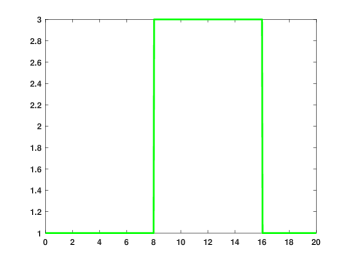
(a) permittivity  index 

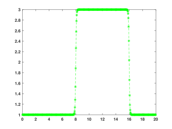
(b) approximate permittivity index

Fig. 1: Permittivity index

However, the matrix $\tilde{\mathbb{Q}}_{v}$ in (6.2) is not sparse, which may affect the complexity of quantum algorithms, and this approach may not simulate the complex media and physical boundary conditions efficiently. We instead consider the Schr$\ddot{\text{o}}$dingerisation combined with the immersed boundary method (or immersed interface method) . For the complex media which has two dielectric material $\Omega^{1}$ with parameters $\varepsilon_{1}$, $\mu_{1}$ and $\Omega_{2}$ with parameters $\varepsilon_{2}$, $\mu_{2}$, and satisfies $\Omega=\Omega_{1}\cup\Omega_{2}$, We define the interface conditions for the electric and magnetic fields on the interface $\Gamma$ are given by

$$\hat{{\bm{n}}}\cdot[\varepsilon{\bm{E}}]=0,\quad\hat{{\bm{n}}}\cdot[{\bm{B}}]=0,\quad\hat{{\bm{n}}}\times[{\bm{E}}]=0,\quad\hat{{\bm{n}}}\times[{\bm{B}}/\mu]=0,\quad\text{on}\,\Gamma,$$ (6.8)

where $\hat{{\bm{n}}}$ is the unit normal of the interface pointing to $\Omega_{1}$ and the jumps on the interface are denoted by

$$[{\bm{E}}]={\bm{E}}|_{\Omega_{1}}-{\bm{E}}|_{\Omega_{2}},\quad[{\bm{B}}]={\bm{B}}|_{\Omega_{1}}-{\bm{B}}|_{\Omega_{2}},\quad\text{on}\,\Gamma.$$ (6.9)

Combining with the interface condition for $\mathcal{F}_{4}$ and $\mathcal{F}_{8}$, i.e.

$$[\mathcal{F}_{4}]=0,\quad[\mathcal{F}_{8}]=0,$$ (6.10)

the jump conditions in terms of the variable $\mathcal{F}$ are

$$R_{1}\mathcal{F}^{1}-R_{2}\mathcal{F}^{2}=\begin{bmatrix}R_{1}^{11}&\textbf{0}\\ \textbf{0}&R_{1}^{22}\end{bmatrix}\mathcal{F}^{1}-\begin{bmatrix}R_{2}^{11}&\textbf{0}\\ \textbf{0}&R_{2}^{22}\end{bmatrix}\mathcal{F}^{2}=\textbf{0},$$ (6.11)

where the matrices $R_{j}^{11}$ and $R_{j}^{22}$, $j=1,2$ are defined by

$$R_{j}^{11}=\begin{bmatrix}\sqrt{\varepsilon_{j}}n_{x}&\sqrt{\varepsilon_{j}}n_{y}&\sqrt{\varepsilon_{j}}n_{z}&1\\ 0&-\frac{n_{z}}{\sqrt{\varepsilon_{j}}}&\frac{n_{y}}{\sqrt{\varepsilon_{j}}}&1\\ \frac{n_{z}}{\sqrt{\varepsilon_{j}}}&0&-\frac{n_{x}}{\sqrt{\varepsilon_{j}}}&1\\ -\frac{n_{y}}{\sqrt{\varepsilon_{j}}}&\frac{n_{x}}{\sqrt{\varepsilon_{j}}}&0&1\\ \end{bmatrix},\quad R_{j}^{22}=\begin{bmatrix}\sqrt{\mu_{j}}n_{x}&\sqrt{\mu_{j}}n_{y}&\sqrt{\mu_{j}}n_{z}&1\\ 0&-\frac{n_{z}}{\sqrt{\mu_{j}}}&\frac{n_{y}}{\sqrt{\mu_{j}}}&1\\ \frac{n_{z}}{\sqrt{\mu_{j}}}&0&-\frac{n_{x}}{\sqrt{\mu_{j}}}&1\\ -\frac{n_{y}}{\sqrt{\mu_{j}}}&\frac{n_{x}}{\sqrt{\mu_{j}}}&0&1\\ \end{bmatrix}.$$

Using the transformation matrix $T$ and unitary matrix $U$, one gets the representation of interface conditions on $\Gamma$ in terms of $\tilde{\Psi}$ as

$$\tilde{R}_{1}\tilde{\Psi}^{1}-\tilde{R}_{2}\tilde{\Psi}^{2}=0,$$ (6.12)

where $\tilde{R}_{j}=RT^{\dagger}U^{\dagger}$. An upwinding embedded boundary method [9] can be applied for the wave equation (5.6) for the space discretization, and then the Schr$\ddot{\text{o}}$dingerisation approach is used for the quantum simulation.

7 Continuous-variable formulation

We remark that the Schrödingerisation framework is not only applicable to qubit-systems, but also to continuous-variable (CV) quantum systems. The continuous-variable analogue of a qubit is a qumode. The Schrödingerisation framework in the qumode representation is introduced in [20].

Unlike a qubit, a CV quantum state, or ‘qumode’, spans an infinite-dimensional Hilbert space. A qumode is the quantum analogue of a continuous classical degree of freedom. A qumode is acted upon by observables with a continuous spectrum, such as the position $\hat{x}$ and momentum $\hat{p}$ observables of a quantum particle. Its eigenbasis can be chosen to be for instance $\{|x\rangle\}_{x\in\mathbb{R}}$, which are the eigenstates of $\hat{x}$. It forms a complete basis so $\int|x\rangle\langle x|=I$. In this basis, a qumode can be expressed as, for instance, $|u(t)\rangle=(1/\|\bm{u}(t)\|)\int u(t,x)|x\rangle dx$, where $\|\bm{u}(t)\|^{2}=\int dx|u(t,x)|^{2}$ is the normalisation constant. A system of $m$-qumodes is a tensor product of $m$ qumodes. The qumode can also be acted upon by quadrature operators like the momentum $\hat{p}$ operator, where $[\hat{x},\hat{p}]=i$.

Maxwell’s equations govern the dynamics of the electric $E_{x,y,z}$ and magnetic fields $B_{x,y,z}$, in the presence of charge density $\rho$ and current density $J_{x,y,z}$. These are all continuous quantities and it is interesting to ask if it is possible to represent this information in a continuous manner in a quantum device without first discretising. This could be made possible through a qumode representation. In addition, it is easy to find from (6.3) that the matrix $\mathbb{Q}_{v}$ is not sparse due to the discretization of varying velocity. However, this defect disappears in a continuous-variable quantum system. It can be seen from (6.2)-(6.3) that the advantages of the matrix representation based on Riemann-Silberstein vectors no longer exists for a linear inhomogeneous medium in our Schrödingerisation framework. Thus we simulate Equation (2.6) instead of Equation (2.8) in this section.

In the qumode representation, vectors $\bm{F}$ in bold, e.g., $\bm{E}_{x,y,z}$, $\bm{B}_{x,y,z}$, $\bm{J}_{x,y,z}$ and $\bm{\rho}$ represents $\bm{F}=\iiint F(x,y,z)|x\rangle|y\rangle|z\rangle dxdydz$, which is a quantum system consisting of 3 qumodes. We define

$$\bm{\mathcal{F}}=\sqrt{\varepsilon}\bm{E}_{x}|0\rangle+\sqrt{\varepsilon}\bm{E}_{y}|1\rangle+\sqrt{\varepsilon}\bm{E}_{z}|2\rangle+\frac{1}{\sqrt{\mu}}\bm{B}_{x}|4\rangle+\frac{1}{\sqrt{\mu}}\bm{B}_{y}|5\rangle+\frac{1}{\sqrt{\mu}}\bm{B}_{z}|6\rangle,$$

$$\bm{\mathcal{J}}=\bm{J}_{x}|0\rangle+\bm{J}_{y}|1\rangle+\bm{J}_{z}|2\rangle-\bm{v}\bm{\rho}|8\rangle,$$

$$\mathcal{D}=\begin{pmatrix}0&i\hat{p}_{z}&-i\hat{p}_{y}&i\hat{p}_{x}\\ -i\hat{p}_{z}&0&i\hat{p}_{x}&i\hat{p}_{y}\\ i\hat{p}_{y}&-i\hat{p}_{x}&0&i\hat{p}_{z}\\ -i\hat{p}_{x}&-i\hat{p}_{y}&-i\hat{p}_{z}&0\end{pmatrix}=-\hat{p}_{z}\otimes\textbf{1}\otimes\sigma_{2}-\hat{p}_{x}\otimes\sigma_{2}\otimes\sigma_{1}+\hat{p}_{y}\otimes\sigma_{2}\otimes\sigma_{3},$$

where $|0\rangle,|1\rangle,...,|8\rangle$ represent the $9$ possible states in the computational basis consisting of 3 qubits. In the continuous-variable framework, we can make the replacement $\partial_{x,y,z}\leftrightarrow-i\hat{p}_{x,y,z}$ where $\hat{p}$ is the momentum operator. In the continuous-variable framework, we can also make the replacement $x\leftarrow\hat{x}$ where $\hat{x}$ is the position operator obeying $[\hat{x},\hat{p}]=i$. Then the following equation governing $\bm{\mathcal{F}}$ with an inhomogeneous term holds:

$$\frac{d\bm{\mathcal{F}}}{dt} =-i\bm{A}\bm{\mathcal{F}}-\bm{\mathcal{J}}$$

$$\bm{A} =-i\sigma_{2}\otimes\frac{v}{2}\mathcal{D}(2I-\bar{\varepsilon}-\bar{\mu})-\sigma_{1}\otimes\frac{v}{2}\mathcal{D}(\bar{\varepsilon}-\bar{\mu}),$$

where $v=v(\hat{x},\hat{y},\hat{z})$, $\bar{\varepsilon}=\bar{\varepsilon}(\hat{x},\hat{y},\hat{z})$ and $\bar{\mu}=\bar{\mu}(\hat{x},\hat{y},\hat{z})$. We define an operator $\hat{\eta}$ such that $\hat{\eta}|\eta\rangle=\eta|\eta\rangle$. One can then apply our Schrödingerisation formulation to the inhomogeneous case. We Schrödingerise the system by dilating $\bm{\mathcal{F}}\rightarrow\bm{y}=\bm{\mathcal{F}}\otimes|0\rangle+\bm{\mathcal{J}}\otimes|1\rangle$ and transform $\bm{y}\rightarrow\tilde{\bm{v}}$ (Schrödingerisation procedure) to obtain the Hamiltonian matrix in (3.11):

$$\bm{H}=\bm{A}_{2}\otimes\frac{1}{2}(\textbf{1}+\sigma_{3})\otimes\hat{\eta}-\frac{\textbf{1}}{2}\otimes\sigma_{1}\otimes\hat{\eta}+\bm{A}_{1}\otimes\frac{1}{2}(\textbf{1}+\sigma_{3})\otimes\textbf{1}+\frac{\textbf{1}}{2}\otimes\sigma_{2}\otimes\textbf{1}=\bm{H}^{\dagger},$$

where $\bm{A}_{1}=(\bm{A}+\bm{A}^{\dagger})/2=\bm{A}_{1}^{\dagger}$, $\bm{A}_{2}=i(\bm{A}-\bm{A}^{\dagger})/2=\bm{A}_{2}^{\dagger}$. This is quantum simulation on a system of 4 qumodes and 4 qubits.

8 Numerical simulation

For the numerical tests, we use the classical computer to simulate Hamilton system to validate the feasibility of the algorithms above. The solution for (3.11) at time $T$ is obtained by

$$\tilde{{\bm{v}}}=e^{-iHT}\tilde{{\bm{v}}}_{0},$$

if $H$ is independent of $t$. Otherwise, the backward Euler method is used to approximate the Hamiltonian system. First we use different quantum algorithms to simulate the propagation of the electromagnetic field without the source term, and then we consider the Schr$\ddot{\text{o}}$dingerisation method applied to physical boundary conditions. Finally, we simulate Maxwell’s equations in media with material interfaces.

8.1 Periodic boundary conditions

In this test, we consider $2D$ Maxwell’s equations in the domain $\Omega=[0,2]^{2}$ for a $z$-transverse magnetic (TM) wave, where the magnetic field ${\bm{B}}$ is transverse to the $z$-direction and electric field ${\bm{E}}$ has only one component along the $z$-direction. We set the cell number as $M=2^{5}$, $N=2^{7}$. The exact solution to the system is

$$E_{z}=\sin(\pi(x+2y+{\sqrt{5}}t)),\quad B_{x}=-2E_{z}/\sqrt{5},\quad B_{y}=E_{z}/\sqrt{5}.$$

(a) $E_{z}$.

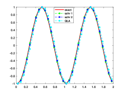
(b) $E_{z}(x^{*},y)$.

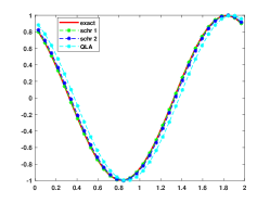
(c) $E_{z}(x,y^{*})$

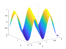
(d) $B_{x}$.

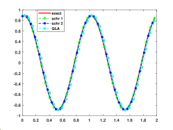
(e) $B_{x}(x^{*},y)$.

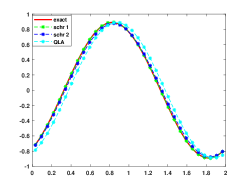
(f) $B_{x}(x,y^{*})$

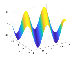
(g) $B_{y}$.

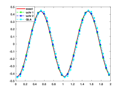
(h) $B_{y}(x^{*},y)$.

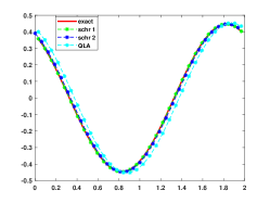
(i) $B_{y}(x,y^{*})$

Fig. 2: Electromagnetic fields at $T=1$ with periodic boundary condition. On the left are the computed solutions with schr1, in the middle and right are the computed and the exact solution with $x^{*}=39/32$ and $y^{*}=7/32$.

	$\triangle\mathcal{E}$	$\triangle(\nabla_{h}\cdot{\bm{B}}_{h})$	$\mathcal{F}_{4,h}$	$\mathcal{F}_{8,h}$	$\text{err}_{EB}$
QLA	1.16e-4	-	3.71e-3	3.72e-3	1.53e-1
schr 1	1.33e-15	-	9.72e-16	9.70e-16	3.72e-15
schr 2	4.44e-16	6.88e-14	-	-	3.83e-2

Tab. 1: Comparation of different schemes.

Simulations of Equation (2.8) are denoted by schr 1, and model (2.5) using the Yee’s algorithm is called schr 2. In Fig. 2, the comparison of schr 1, schr 2 and QLA proposed in [34, 35] shows that they are very close to the exact solution, and schr 1 ends up superior. Define the discrete energy as

$$\mathcal{E}(T)=\sum_{{\bm{j}}}(E_{z,{\bm{j}}}^{2}+B_{x,{\bm{j}}}^{2}+B_{y,{\bm{j}}}^{2})\triangle x^{2}.$$

From Table 1, we find that the values of $\triangle\mathcal{E}=|\mathcal{E}(T)-\mathcal{E}(0)|$ and $\triangle(\nabla_{h}\cdot{\bm{B}}_{h})=|\nabla_{h}\cdot{\bm{B}}_{h}(t)-\nabla_{h}\cdot{\bm{B}}_{h}(0)|$ are close to zero for schr 2 even when $\text{err}_{EB}$ is much bigger, where $\text{err}_{EB}$ is the error between the numerical and exact electromagnetic fields denoted by

$$\text{err}_{EB}=\max_{{\bm{j}}}\big{(}|E_{z,{\bm{j}}}-E_{z}({\bm{x}}_{{\bm{j}}},T)|\;|B_{x,{\bm{j}}}-B_{x}({\bm{x}}_{{\bm{j}}},T)|\;|B_{y,{\bm{j}}}-B_{y}({\bm{x}}_{{\bm{j}}},T)|\big{)}.$$

Let $\mathcal{F}_{4,h}$ denote the approximation of $\mathcal{F}_{4}$, which is the error of the Maxwell-Thomson equation. We find $\|\mathcal{F}_{4,h}\|_{l^{\infty}}\sim\text{err}_{EB}$ for schr 1 and QLA.

8.2 Physical boundary conditions with source terms

For simplicity of the exposition, we restrict ourselves to a reduced version of the Maxwell equations with one spatial variable, $x$, namely Equation (5.4). Moreover we assume $\sqrt{\varepsilon}=\sqrt{\mu}=1$. Let us consider a 1D case in $[0,L]$ with $L=15$, and use the exact solution to test the accuracy of algorithm. The cell number is set by $M=2^{6}$, $N=2^{7}$. The simulation stops at $T=1$. The perfect conductor boundary condition for the TE model reads as

$$E_{y}(0)=0,\quad E_{y}(L)=0.$$ (8.1)

In order to enforce the boundary condition, we set the exact solution as

$$E_{x}=\sin(2\pi(x+t)/5),\quad E_{y}=\frac{2\pi}{5}(\cos(2\pi x/5)/(2\pi)-1),\quad B_{z}=t\sin(2\pi x/5).$$ (8.2)

Using the same method in (5.7), we get the perfect conductor boundary condition on the right side of the domain for Equation (5.6)

$$\begin{bmatrix}\tilde{\psi}_{1}\\ \tilde{\psi}_{3}\\ \tilde{\psi}_{5}\\ \tilde{\psi}_{7}\end{bmatrix}=\frac{1}{2\sqrt{2}}\begin{bmatrix}1&-1&1&1\\ 1&-1&-1&-1\\ 1&1&1&-1\\ -1&-1&1&-1\end{bmatrix}\begin{bmatrix}\tilde{\psi}_{0}\\ \tilde{\psi}_{2}\\ \tilde{\psi}_{4}\\ \tilde{\psi}_{6}\end{bmatrix}=B_{O2E}\begin{bmatrix}\tilde{\psi}_{1}\\ \tilde{\psi}_{3}\\ \tilde{\psi}_{5}\\ \tilde{\psi}_{7}\end{bmatrix}.$$ (8.3)

Changing the matrix $B_{O2E}$ in (5.12), one gets the system for the Hamiltonian simulation with the perfect conductor boundary of the domain. The results are shown in Fig. 3.

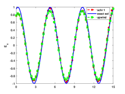
(a) $E_{x}$

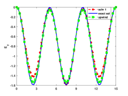
(b) $E_{y}$

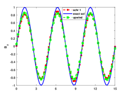
(c) $B_{z}$

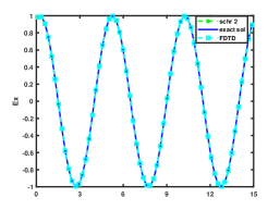
(d) $E_{x}$

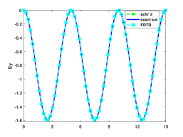
(e) $E_{y}$

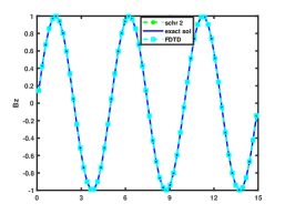
(f) $B_{z}$

Fig. 3: Results for $T=1$ with perfect conductor boundaries. The first row are the simulations using upwind algorithm and the second row using Yee’s algorithm.

In the 1D case, the impedance boundary condition reads

$$E_{y}(0)+vB_{z}(0)=0,\quad vB_{z}(L)-E_{y}(L)=0.$$ (8.4)

We set the source term and the initial value carefully such that the solution satisfies

$$E_{x}=-\sin(\pi(x+t)/5),\quad E_{y}=5\cos(\pi x/5)/\pi,\quad B_{z}=t\sin(\pi x/5)-5/\pi.$$ (8.5)

Similar to (8.3), one gets the left impedance boundary condition of the domain for Equation (5.6),

$$\begin{bmatrix}\tilde{\psi}_{0}\\ \tilde{\psi}_{2}\\ \tilde{\psi}_{4}\\ \tilde{\psi}_{6}\end{bmatrix}=\frac{1}{2\sqrt{2}}\begin{bmatrix}1&1&-\frac{v-1}{v+1}&\frac{v-1}{v+1}\\ -1&-1&-\frac{v-1}{v+1}&\frac{v-1}{v+1}\\ -\frac{v-1}{v+1}&\frac{v-1}{v+1}&1&1\\ -\frac{v-1}{v+1}&\frac{v-1}{v+1}&-1&-1\\ \end{bmatrix}\begin{bmatrix}\tilde{\psi}_{1}\\ \tilde{\psi}_{3}\\ \tilde{\psi}_{5}\\ \tilde{\psi}_{7}\end{bmatrix}=B_{E2O}\begin{bmatrix}\tilde{\psi}_{1}\\ \tilde{\psi}_{3}\\ \tilde{\psi}_{5}\\ \tilde{\psi}_{7}\end{bmatrix}.$$ (8.6)

By replacing the matrix $B_{E2O}$ in (5.12), one obtains the ODE system for the quantum simulation.

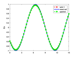
(a) $E_{x}$

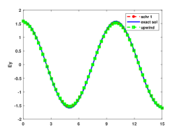
(b) $E_{y}$

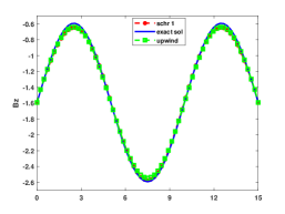
(c) $B_{z}$

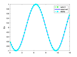
(d) $E_{x}$

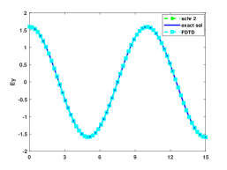
(e) $E_{y}$

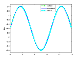
(f) $B_{z}$

Fig. 4: Results for $T=1$ with impedance boundary conditions. The first row are the simulations using upwind algorithm and the second row using Yee’s algorithm.

Comparing with the figures in Fig. 3 and Fig. 4, it can be seen that Schr$\ddot{\text{o}}$dingerisa-tion with both upwind algorithm and Yee’s method can match the boundary conditions very well. Since the upwind scheme only has a first order accuracy of spatial discretization, the later is closer to the exact solution while using the same mesh size.

8.3 Simulations in inhomogeneous medium

Here, we simulate the evolution of a Gaussian pulse form a medium with $\varepsilon_{1}=1$, $\mu_{1}=1$ to the other with $\varepsilon_{2}=3$, $\mu_{2}=1$, the discontinue parameter $\varepsilon$ and its approximation are shown in Fig. 1. The initial electromagnetic pulse is given by

$$E_{y}(x,0)=B_{z}(x,0)=0.01\exp\big{[}-\frac{20(x-3)^{2}}{100}\big{]}.$$ (8.7)

In Fig. 5, the first row are the results of Schr$\ddot{\text{o}}$dingerisation approach with $M=N=2^{7}$ and the second row are the approximation of QLA [34, 35] with fine mesh $M=2^{11}$, which shows that the numerical solutions from Schr$\ddot{\text{o}}$dingerisation method are in agreement with the ones of QLA .

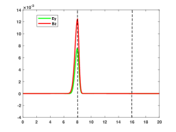
(a) $t=5$

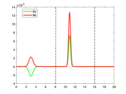
(b) $t=10$

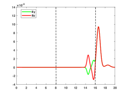
(c) $t=19.5$

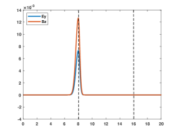
(d) $t=5$

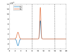
(e) $t=10$

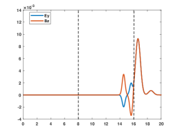
(f) $t=19.5$

Fig. 5: Approximation of electromagnetic fields with schr 1 and QLA algorithm .

Next we verify the accuracy of the Schr$\ddot{\text{o}}$dingerisation approach combined with the IIM method for Equation (5.6) with the jump conditions in (6.12) . The medium is divided into two parts–the medium on the left $(-9\leq x\leq 0)$ is vacuum ($\varepsilon_{1}=\mu_{1}=1$), the right $(0\leq x\leq 10)$ is a dielectric with $\varepsilon_{2}=\mu_{2}=2$ [26]. The incident plane is

$$E_{y,\text{inc}}=\exp{[i(\omega t-k_{1}x)]},\quad B_{z,\text{inc}}=\exp{[i(\omega t-k_{1}x)]}/v_{1},$$ (8.8)

where $\omega=0.5$, $v_{1}=1/\sqrt{\varepsilon_{1}\mu_{1}}$, $k_{i}=\omega\sqrt{\varepsilon_{i}\mu_{i}}$ and $Z_{i}=\sqrt{\mu_{i}/\varepsilon_{i}}$, $i=1,2$. A reflective and transmitted wave will be generated when the incident wave encounters the interface. The boundary conditions are chosen such that the exact solutions satisfy

$$E_{y}(x,t) =\begin{cases}\exp{[i(\omega t-k_{1}x)]}+\frac{Z_{2}-Z_{1}}{Z_{1}+Z2}\exp{[i(\omega t+k_{1}x)]}\quad x<0\\ \frac{2Z_{2}}{Z_{1}+Z_{2}}\exp{[i(\omega t-k_{2}x)]}\quad x>0,\end{cases}$$

$$B_{z}(x,t) =\begin{cases}\frac{1}{v_{1}}\exp{[i(\omega t-k_{1}x)]}-\frac{Z_{2}-Z_{1}}{v_{1}(Z_{1}+Z2)}\exp{[i(\omega t+k_{1}x)]}\quad x<0,\\ \frac{2\mu_{2}}{Z_{1}+Z_{2}}\exp{[i(\omega t-k_{2}x)]}\quad x>0,\end{cases}$$

The mesh size is set by $M=N=2^{7}$. As shown in Fig. 6, the Schr$\ddot{\text{o}}$dingerisation method captures the jump conditions across the material interface well, and its approximation is close to the exact solution.

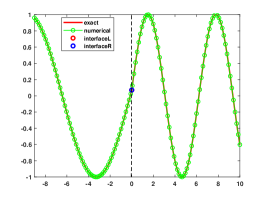
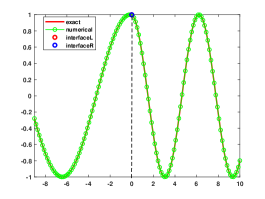
(a) $E_{y}$

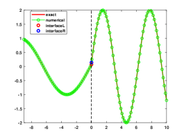
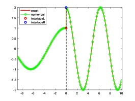
(b) $B_{z}$

Fig. 6: Electromagnetic fields at $T=3$.

9 Conclusions

In this paper, we propose quantum algorithms for Maxwell’s equations, using the Schr$\ddot{\text{o}}$dingerisation method introduced in [22, 23]. The proposed method has been demonstrated for the eight-dimensional matrix representation of Maxwell’s equations based on the Riemann-Silberstein vectors, and to electromagnetic models based on electric and magnetic fields. While source terms and physical boundary conditions are natural in simulations, quantum simulation incorporating these conditions are difficult due to the lack of unitarity of these systems. We give implementation details for three physical boundary conditions, including periodic, perfect conductor and impedance boundary conditions. In addition, we simulate Maxwell’s equations in a linear inhomogeneous medium with interface conditions. Finally, we touch upon continuous-variable quantum systems to simulate Maxwell’s equations via Schr$\ddot{\text{o}}$dingerisation.

We did not consider the treatment of quantum simulations algorithms for Maxwell’s equations in unbounded domains. As pointed out in [21], the Schr$\ddot{\text{o}}$dingerisation method can be applied to quantum dynamics with artificial boundary conditions. These will be the subject of our future research.

References

- [1] D. An, D. Fang, and L. Lin. Time-dependent unbounded hamiltonian simulation with vector norm scaling. Quantum, 5(459), 2021.
- [2] D. An, D. Fang, and L. Lin. Time-dependent hamiltonian simulation of highly oscillatory dynamics and superconvergence for schrödinger equation. Quantum, 6(690), 2022.
- [3] F. Assous, P. Ciarlet, and S. Labrunie. Mathematical foundations of computational electromagnetism. Springer International Publishing AG, 2018.
- [4] D. W. Berry, A. M. Childs, and R. Kothari. Hamiltonian simulation with nearly optimal dependence on all parameters. IEEE 56th annual symposium on foundations of computer science, 2015.
- [5] D. W. Berry, A. M. Childs, Y. Su, X. Wang, and N. Wiebe. Time-dependent hamiltonian simulation with l1-norm scaling. Quantum, 4(254), 2020.
- [6] N. Bui, A. Reineix, and C. Guiffaut. Alternative quantum circuit implementation for 2d electromagnetic wave simulation with quasi-pec modeling. IEEE MTT-S International Conference on Electromagnetic and Multiphysics Modeling and Optimization, 2022.
- [7] L. Cai, Meng F. X., and X.T. Yu. Quantum algorithm for method of moment in electromagnetic computation. IEEE International Conference on Microwave and Millimeter Wave Technology (ICMMT), pages 1–3, 2021.
- [8] W. Cai. Computational Methods for Electromagnetic Phenomena: electrostatics in solvation, scattering, and electron transport. Cambridge University Press, 2013.
- [9] W. Cai and S. Deng. An upwinding embedded boundary method for maxwell’s equations in media with material interfaces: 2d case. J. Comput. Phys., 190(1):159–183, 2003.
- [10] B. D. Clader, B. C. Jacobs, and C. R. Sprouse. Preconditioned quantum linear system algorithm. Phys. Rev. Lett., 110(25):250504, 2013.
- [11] P. C. Costa, S. Jordan, and A. Ostrander. Quantum algorithm for simulating the wave equation. Phys. Rev. A, 99(1):012323, 2019.
- [12] D. Deutsch. Quantum theory, the church-turing principle and the universal quantum number. Proc. Roy. Soc. Lon. A, 400(1818):97–117, 1985.
- [13] D. DiVincenzo. Quantum computation. Science, 270(5234):255–261, 1995.
- [14] A. Ekert, R. Jozsa, and P. Marcer. Quantum algorithms: Entanglement-enhanced information processing. Philos. Trans. Royal Soc. A, 356(1743):1769–1782, 1998.
- [15] D. Fang, L. Lin, and Y. Tong. Time-marching based quantum solvers for time-dependent linear differential equations. Quantum, 7(955), 2023.
- [16] R. Feynman. Simulating physics with computers. Int. J. Theor. Phys., 21(6):467–488, 1982.
- [17] M. Freiser and P. Marcus. A survey of some physical limitations on computer elements. IEEE Trans. Magn., 5(2):82–90, 1969.
- [18] G. H. Golub and C. F. V. Loan. Matrix Computations. Johns Hopkins University Press, 1996.
- [19] S. Jin, X. Li, N. Liu, and Y. Yu. Quantum simulation for partial differential equations with physical boundary or interface conditions. arXiv:2305.02710.
- [20] S. Jin and N. Liu. Analog quantum simulation of partial differential equations. arXiv:2308.00646, 2023.
- [21] S. Jin, N. Liu, X Li, and Y. Yu. Quantum simulation for quantum dynamics with artificial boundary conditions. arXiv:2304.00667, 2023.
- [22] S. Jin, N. Liu, and Y. Yu. Quantum simulation of partial differential equations via schrodingerisation. arXiv preprint arXiv:2212.13969., 2022.
- [23] S. Jin, N. Liu, and Y. Yu. Quantum simulation of partial differential equations via schrodingerisation: technical details. arXiv preprint arXiv:2212.14703, 2022.
- [24] A. S. Khan. An exact matrix representation of maxwell’s equations. Phys. Scripta, 71(5):440, 2005.
- [25] S. A. Khan and R. Jagannathan. A new matrix representation of the maxwell equations based on the riemann-silberstein-weber vector for a linear inhomogeneous medium. arxiv.org/abs/2205.09907, 2022.
- [26] P. Lorrain and F. Lorrain. Electromagnetics Fields and Waves. W.H. Freeman and Company, New York, 1988.
- [27] M. A. Nielsen and I. L. Chuang. Quantum Computation and Quantum Information. Cambridge University Press, 2000.
- [28] P.W. Shor. Algorithms for quantum computation: discrete logarithms and factoring. In: Proceedings of 35th Annual Symposium on Foundations of Computer Science, pages 124–134, 1994.
- [29] A. Steane. Quantum computing. Rep. Progr. Phys., 61(2):117–173, 1998.
- [30] A. Suau, G. Staffelbach, and H. Calandra. Practical quantum computing: Solving the wave equation using a quantum approach. ACM Trans. Quantum Comput., 2(1):1–35, 2021.
- [31] A. Taflove, S. C. Hagness, and M. Piket-May. Computational electromagnetics: the finite-difference time-domain method. The Electrical Engineering Handbook, 3:629–670, 2005.
- [32] G. Vahala, L. Vahala, M. Soe, and A. K. Ram. The effect of the pauli spin matrices on the quantum lattice algorithm for maxwell equations in inhomogeneous media. 10.48550/arXiv.2010.12264, 2020.
- [33] G. Vahala, L. Vahala, M. Soe, and A. K. Ram. Unitary quantum lattice simulations for maxwell equations in vacuum and in dielectric media. J. Plasma. Phys., 86(5):905860518, 2020.
- [34] G. Vahala, L. Vahala, M. Soe, and A. K. Ram. One- and two-dimensional quantum lattice algorithms for maxwell equations in inhomogeneous scalar dielectric media i: theory. Radiat. Eff. Defect. S., 176(1):49–63, 2021.
- [35] G. Vahala, L. Vahala, M. Soe, and A. K. Ram. One- and two-dimensional quantum lattice algorithms for maxwell equations in inhomogeneous scalar dielectric media ii: simulations. Radiat. Eff. Defect. S., 176(2):64–72, 2021.
- [36] J. Yepez. An efficient and accurate quantum algorithm for the dirac equation. arXiv preprint quant-ph/0210093, 2002.
- [37] J. Zhang, F. Feng, and Q. J. Zhang. Quantum method for finite element simulation of electromagnetic problems. IEEE MTT-S International Microwave Symposium (IMS), pages 120–123, 2021.