Availability, storage capacity, and diffusion: Stationary states of an asymmetric exclusion process connected to two reservoirs

Abstract

We explore how the interplay of finite availability, carrying capacity of particles at different parts of a spatially extended system and particle diffusion between them control the steady state currents and density profiles in a one-dimensional current-carrying channel connecting the different parts of the system. To study this, we construct a minimal model consisting of two particle reservoirs of finite carrying capacities connected by a totally asymmetric simple exclusion process (TASEP). In addition to particle transport via TASEP between the reservoirs, the latter can also directly exchange particles, modeling particle diffusion between them that can maintain a steady current in the system. We investigate the steady state density profiles and the associated particle currents in the TASEP lane. The resulting phases and the phase diagrams are quite different from an open TASEP, and are characterised by the model parameters defining particle exchanges between the TASEP and the reservoirs, direct particle exchanges between the reservoirs, and the filling fraction of the particles that determines the total resources available. These parameters can be tuned to make the density on the TASEP lane globally uniform or piecewise continuous, and can make the two reservoirs preferentially populated or depopulated.

I INTRODUCTION

Driven diffusive systems have emerged as fascinating subjects of research in nonequilibrium physics, providing fertile ground for investigations of the fundamental issues of nonequilibrium steady states (NESS) and phase transitions driven-diff1 ; driven-diff2 ; driven-diff3 ; driven-diff4 . Even in one dimension (1D), driven diffusive systems can exhibit nontrivial properties with just local dynamics at the microscopic level. One of the most prominent examples is the totally asymmetric simple exclusion process (TASEP) krug ; krug1 ; krug2 ; derrida . A TASEP consists of a 1D lattice with open boundaries. The dynamics is stochastic in nature, and involves unidirectional particle hopping, subject to exclusion at all the sites, i.e., any site can contain at most one particle. In TASEP dynamics, a particle enters at one of the boundaries at a specified rate, unidirectionally hops to the following sites at rate unity subject to exclusion until it reaches the other end, from which it leaves at another specified rate. Parametrised by the entry and exit rates at the boundary, the TASEP exhibits three distinct phases: the steady state densities in bulk can be either less than half, giving the low-density (LD) phase, or more than half, giving the high-density (HD) phase, or just half, which is the maximal current (MC) phase. Alongside these uniform phases, a coexistence line (CL) separating the LD and HD phases can also be observed where nonuniform densities in the form of domain wall (DW) can be found. This DW is delocalised in space, attributed to the particle nonconservering dynamics governing the open TASEP.

Originally, the TASEP was proposed as a simple model to describe protein synthesis in biological cells macdonald . Subsequently, it was reinvented as a paradigmatic nonequilibrium model when it was discovered to have boundary-induced phase transitions krug ; krug1 ; krug2 .

In the present study, our focus is on a different class of TASEP models without open boundaries, in which a single TASEP is connected to a particle reservoir at both ends, i.e., a TASEP has a “restricted” or “finite access” to resources of particles. In order to ensure a finite steady current in the nonequilibrium steady states, the two reservoirs are allowed to exchange particles at given specified rates instantaneously, which models particle diffusion. Clearly, this puts a constraint on the total number of particles in the combined system of the TASEP and the attached reservoirs, which is held constant by the dynamics. This is principally motivated by biological and physical processes that are often under the constraint of limited resources, which necessitates the study of closed lattice models. For instance, TASEPs with finite resources provide a simple description of the basic mechanism for the biological processes of protein synthesis in cells reser1 , due to the finite amount of ribosomes available in a cell, and also in the context of traffic traffic1 , due to the finite number of automobiles in a network of roads; see also Ref. limited in this context. Some of the examples of the applications of a TASEP connected to a reservoir are limited resources in driven diffusive systems lim-driv , different biological contexts like mRNA translations and motor protein dynamics in cells lim-bio1 and traffic problems lim-bio2 . Notable experiments relevant to these model systems include studies on spindles in eukaryotic cells lim-exp1 ; lim-exp2 .

A TASEP connected with a reservoir conserves particle number globally, i.e., on the TASEP and reservoir as a whole reser1 ; reser2 , but not on the TASEP itself, giving an overall particle number conservation (PNC). In the existing studies on TASEP with closed geometry, the actual particle entry rates, unlike open TASEPs, depend upon the instantaneous reservoir population; the exit rates are usually assumed to be constants, similar to open TASEPs. In general, a closed system consisting of a TASEP and a reservoir manifestly breaks the translation invariance and hence is a potential candidate for macroscopically inhomogeneous steady state densities. How the finite pool of available particles affect the steady state occupations and currents in comparison with open TASEPs is the key qualitative question in all these studies.

At the basic level of modeling of a TASEP with finite resources, a single TASEP is connected at both ends to a particle reservoir without any spatial extensions (i.e., a point reservoir), with the entry rate to the TASEP from the reservoir being given by a function of the instantaneous reservoir occupation; the exit rate from the TASEP to the reservoir is taken to be constant, as in an open TASEP. This has been generalised to more than one TASEP connected to a reservoir as a model to study competition between TASEPs for finite resources; see Ref. reser3 . Detailed numerical stochastic simulations and analytical mean-field theory studies reveal rich nonuniform steady state density profiles, including domain walls in these models reser1 ; reser2 ; reser3 . In another interesting extension of a TASEP with finite resources, the effect of a limited number of two different fundamental transport resources, viz. the hopping particles and the “fuel carriers”, which supply the energy required to drive the system away from equilibrium has been considered in Ref. brackley that reports multiple phase transitions as the entry and exit rates are changed. It may be noted that in all these studies on TASEPs with finite resources, the effective entry rate of the particles from the reservoir to the TASEP lane is not constant but depends on the instantaneous reservoir population. In a recent study astik-1tasep , both the entry and exit rates are assumed to depend on the instantaneous reservoir population leading to dynamics-induced competition between the entry and exit rates, which reveals reservoir crowding effects on the steady states.

Diffusion is ubiquitous in nature, in particular, in cell biological contexts diff-cell . In a cell, molecular motors can undergo driven motion along the microtubules, which are effectively 1D channels, or diffusion in the cell cytoplasm. This opens up the question of possible competition between diffusion and driven motions. Studies on competition between symmetric exclusion process, a representation of 1D diffusion and TASEP is relatively rare. Notable examples include Refs. hinsch ; anjan-parna , where an overall closed system has been considered, and Ref. sm , where it has been studied in a system with open boundaries. Nonetheless, systematic studies on the mutual interplay between driven and diffusive motion together with finite resources are still lacking.

In spite of the significant development in researches on TASEP with finite resources, there are many questions or issues which remain largely unexplored. In more realistic situations, resources may be “distributed”, a reflection of closed but spatially extended systems. Such distributed resources may be connected by channels carrying steady currents, which can be tuned by both the “supply side” as well as the “receiving side”. Furthermore, such distributed resources may also diffusively exchange particles between them, which can compete with the particle flow in the current carrying channels.

The overarching goal of the present study is to theoretically study and understand the nonequilibrium steady states in systems with multiple reservoirs representing distributed resources having finite capacities. We consider two such reservoirs connected by a single current carrying channel executing TASEP dynamics, and exchanging particles at given specified rates which model diffusion. The model naturally ensures a steady current in the TASEP channel. Overall particle number conservation is imposed. This provides a simple conceptual model for a system with multiple distributed resources exchanging particles through diffusion and connected by channels with steady currents. We study two specific limits of the model, when the particles exchange process competes with the current in the TASEP channel, and a second case when the former overwhelms the TASEP current. We show that for appropriate choice of the model parameters, the TASEP density profile can be spatially uniform, or display macroscopic nonuniformity in the form of a localized domain wall (LDW). The relative populations of the two reservoirs can also be controlled dynamically.

The rest of the article is organised as follows: In Section II, we provide a brief description of the model. Section III presents a mean-field analysis of its nonequilibrium steady state properties. Next, in Section IV, we present the phase diagrams when the particle exchange competes with the TASEP current, called the weak coupling limit. The density profiles and boundaries between different phases are determined within the framework of MFT in Section V. Particle-hole symmetry is discussed in Section VI, followed by an exploration of the nature of phase transitions in Section VII. Finally, we summarise our findings and provide an outlook in Section VIII. Additional details including results on the case when the particle exchange dominates, called the strong coupling limit, are given in Appendix.

II MODEL

The model consists of a 1D lattice $T$ with $L$ number of sites, which executes TASEP dynamics and is connected to two particle reservoirs $R_{1}$ and $R_{2}$, having finite particle storage capacities; see Fig. 1 for a schematic diagram of the model. The reservoirs are assumed to be point reservoirs without any spatial extent or internal dynamics. The sites of $T$ are labeled by an index $i$, $i\in[1,L]$ with $i=1(L)$ as the entry(exit) end, and can accommodate no more than one particle at a given time. Particles enter $T$ from the left reservoir $R_{1}$ provided the first site of $T$ is empty, hop uni-directionally along $T$ subject to hard-core exclusion, i.e., only if the next site is vacant, and eventually leave $T$ to enter thr right reservoir $R_{2}$. We choose the hopping rate in the bulk of $T$ as unity, which sets the time scale of the model. Our model strictly follows particle number conservation (PNC) globally, which reads

$$N_{0}=N_{1}+N_{2}+\sum_{i=1}^{L}n_{i},$$ (1)

where $N_{0}$ is the total particle number of the system (reservoirs and TASEP lane combined), $N_{1}$ and $N_{2}$ are the particle numbers in $R_{1}$ and $R_{2}$, respectively, and $n_{i}\in 0$ or $1$, denotes the occupation number of site $i$ in the TASEP lane. The entry and exit rates are parametrised by $\alpha$ and $\beta$, which may take any positive value. Actual entry and exit rates, which should also be positive, depend on the instantaneous reservoir population and are given by

$$\alpha_{\text{eff}}=\alpha f(N_{1}),\hskip 14.22636pt\beta_{\text{eff}}=\beta g(N_{2})$$ (2)

These rates model the coupling of the $T$ with its “environments”, i.e., the two reservoirs. It is reasonable to expect that a rising population of $R_{1}$ ($R_{2}$) facilitates (obstructs) the inflow (outflow) of particles to (from) $T$. In keeping with this expectation, $f$ and $g$ are assumed to be monotonically increasing and decreasing functions of $N_{1}$ and $N_{2}$ respectively. We make the following simple choices:

$$f(N_{1})=\frac{N_{1}}{L},\hskip 14.22636ptg(N_{2})=1-\frac{N_{2}}{L},$$ (3)

where these reservoir population-dependent rate functions $f$ and $g$ must be positive to make the effective rates in (2) positive. The positivity of $g$ in (3) requires the restriction $N_{2}\leq L$. While more complex forms for monotonically rising $f$ and decreasing $g$ can be conceived, such simple choices as given in (3) suffice for the present purposes. Since the particle current through $T$ is unidirectional from $R_{1}$ to $R_{2}$, in order to maintain a steady non-zero current, there must be another mechanism for particle exchanges between $R_{1}$ and $R_{2}$. To that end, we allow the reservoirs to exchange of particles directly, modelling diffusion between them, at some fixed rates: $R_{1}(R_{2})$ releases particles at rate $k_{1}(k_{2})$ which $R_{2}(R_{1})$ receives instantaneously. We further define filling factor by $\mu=N_{0}/L$. Taken together, our model has five control parameters — $\alpha$, $\beta$, $\mu$, $k_{1}$, and $k_{2}$ — which determine the steady states of the model.

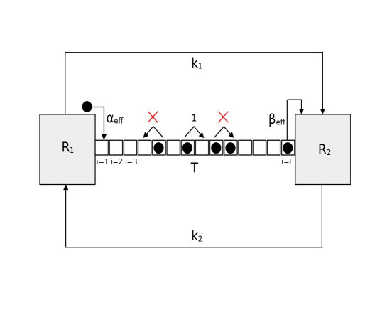
Figure 1: Schematic model diagram: The diagram illustrates the system configuration consisting of two reservoirs $R_{1}$ and $R_{2}$, with $N_{1}$ and $N_{2}$ number of particles, respectively which are connected by a TASEP lane, denoted as $T$, having $L$ sites. Particles, which are denoted by black solid circles, enter the first site ($i=1$) of $T$ from $R_{1}$ with an effective rate $\alpha_{\text{eff}}$ and hop from left to right with rate 1 subject to exclusion. Eventually, particles are removed from the last site ($i=L$) of $T$ into $R_{2}$ with an effective rate of $\beta_{\text{eff}}$. Additionally, particle exchanges occur directly between $R_{1}$ and $R_{2}$ with rates $k_{1}$ and $k_{2}$ modelling diffusion into the system.

III MEAN-FIELD THEORY

In this Section, we analyse the model at the mean-field level following same line of reasoning as in earlier works blythe . MFT entails neglecting the correlation effects and replacing averages of products by the products of averages. In the mean-field description, the equations of motion for the density $\rho_{i}(t)$ at site $i$ are

$$\frac{d\rho_{i}}{dt}=\rho_{i-1}(1-\rho_{i})-\rho_{i}(1-\rho_{i+1}),\,i=2,..,L-1,$$ (4)

$$\frac{d\rho_{1}}{dt}=\alpha_{\text{eff}}(1-\rho_{1})-\rho_{1}(1-\rho_{2}),$$ (5)

$$\frac{d\rho_{L}}{dt}=\rho_{L-1}(1-\rho_{L})-\beta_{\text{eff}}\rho_{L}.$$ (6)

Similarly, the the reservoir populations $N_{1}$ and $N_{2}$ follow

$$\frac{dN_{1}}{dt}=k_{2}N_{2}-k_{1}N_{1}-J_{T},$$ (7)

$$\frac{dN_{2}}{dt}=k_{1}N_{1}-k_{2}N_{2}+J_{T}.$$ (8)

In what follows below, for the convenience of presenting our results, we assume unit geometric length of the lattice, introduce a quasi-continuous variable $x=i/L\in[0,1]$ where $\epsilon=1/L$ is the lattice constant. With this new coordinate $x$, the discrete density $\rho_{i}(t)$ is replaced by a continuous density $\rho(x,t)$. The equation of motion of $\rho(x,t)$ in the bulk of $T$ reads blythe

$$\frac{\partial\rho(x)}{\partial t}=-\epsilon\partial_{x}(\rho(x)[1-\rho(x)])+{\cal O}(\epsilon^{2}),$$ (9)

supplemented by the boundary conditions $\rho(0)=\alpha_{\text{eff}},\,\rho(1)=1-\beta_{\text{eff}}$. Eq. (9) has a conservation law form, reflecting the conserving nature of the TASEP dynamics in the bulk, and thus allows us to extract a particle current $J_{T}$ that in the MFT has the form

$$J_{T}=\rho(1-\rho).$$ (10)

This current $J_{T}$ is related to the reservoir occupation numbers, $N_{1}$ and $N_{2}$, through a flux balance equation in the steady state:

$$\frac{dN_{1}}{dt}=k_{2}N_{2}-k_{1}N_{1}-J_{T}=-\frac{dN_{2}}{dt}=0.$$ (11)

Moreover, PNC imposes the constraint

$$N_{0}=N_{1}+N_{2}+N_{T}.$$ (12)

In the steady states, $\partial\rho/\partial t=0$, giving $J_{T}$ a constant. For a given constant current $J$, the possible steady state densities in TASEP are

$$\rho=\frac{1}{2}\left(1\pm\sqrt{1-4J}\right)=:\rho_{\pm}.$$ (13)

Thus the steady state TASEP density can be spatially uniform with $\rho=\rho_{-}\leq 1/2$ (LD phase), or $\rho=\rho_{+}>1/2$ (HD phase). In the particular case when $J$ is at its maximum value $J=1/4$, $\rho=1/2$ (MC phase). There is also a second possibility in which case $\rho$ is piecewise discontinuous, with $\rho=\rho_{-}$ and $\rho=\rho+$ occurring at different regions of $T$. This gives rise to a domain wall (DW).

Our model admits a special symmetry, called the particle-hole symmetry when $k_{1}=k_{2}$. The transformations

$$\rho_{i}\leftrightarrow 1-\rho_{L-(i-1)},$$ (14)

$$\alpha_{\text{eff}}\leftrightarrow\beta_{\text{eff}},$$ (15)

leave Eqs. (4-6) invariant. Also, since $\alpha_{\text{eff}}=\alpha N_{1}/L$ and $\beta_{\text{eff}}=\beta(1-N_{2}/L)$, transformation (15) can be decomposed into two parts: $\alpha\leftrightarrow\beta$ together with $N_{1}/L\leftrightarrow(1-N_{2}/L)$. These properties allow us to obtain the phase diagrams of our model for $\mu>3/2$ (greater than the half-filled limit) from those at $\mu<3/2$ (less than the half-filled limit) when $k_{1}=k_{2}$ (discussed later). For $k_{1}\neq k_{2}$, there is no such symmetry.

In the steady state, $dN_{1}/dt=0=dN_{2}/dt$, and hence flux balance condition (11) gives

$$k_{2}N_{2}=k_{1}N_{1}+J_{T}.$$ (16)

Solving eq. (11) together with (12), we get the following expressions for the reservoir populations:

$$N_{1}=\frac{k_{2}(N_{0}-N_{T})-J_{T}}{k_{1}+k_{2}},$$ (17a)

$$N_{2}=\frac{k_{1}(N_{0}-N_{T})+J_{T}}{k_{1}+k_{2}}.$$ (17b)

After determining the reservoir populations, our next task is to calculate the maximum of the filling factor $\mu\equiv N_{0}/L$. We have $\mu=0$, its minimum value, when there are no particles present in the system. Consequently, in the TASEP, this implies a steady state particle density of zero. When $\mu$ reaches its maximum value $\mu_{\text{max}}$, the particle density in the TASEP lane is equal to 1. Hence, the particle current becomes zero since there is no available space for particles to flow within the completely filled system. Eqs. (17a) and (17b) imply

$$\frac{N_{1}}{N_{2}}=\frac{k_{2}}{k_{1}},$$ (18)

which gives

$$N_{1_{\text{max}}}=\frac{k_{2}}{k_{1}}N_{2_{\text{max}}}=\frac{k_{2}L}{k_{1}}.$$ (19)

Additionally, the number of particles in the TASEP lane is $N_{T}=L$ when $\mu=\mu_{\text{max}}$. By substituting these values into the PNC relation (12), we determine the upper limit of $\mu$ as

$$\mu_{\text{max}}=\bigg{(}2+\frac{k_{2}}{k_{1}}\bigg{)}.$$ (20)

Thus, $\mu_{\text{max}}$ is controlled by the exchange rate ratio $k_{2}/k_{1}$. Since $k_{2}/k_{1}$ itself varies between 0 (when $k_{2}=0$ or $k_{2}<<k_{1}$) and $\infty$ (when $k_{1}=0$ or $k_{1}<<k_{2}$), the upper limit of $\mu$ is not fixed and can be any number between 2 and $\infty$. In the particular case, when the exchange rates are equal, the value of $\mu_{\text{max}}$ is 3. At this point, the transformation $\mu\leftrightarrow 3-\mu$ captures the particle-hole symmetry of the model. See Fig. 2 for a state diagram of the model in the $k_{2}/k_{1}-\mu$ plane.

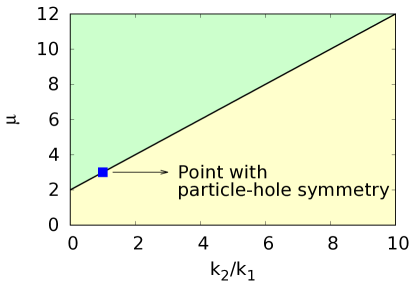
Figure 2: State diagram of the model in the $k_{2}/k_{1}-\mu$ plane. The black inclined line given by $\mu=\mu_{\text{max}}=(2+k_{2}/k_{1})$ gives the maximum possible filling fraction admissible for a given $k_{2}/k_{1}$. In the yellow region below the black line one has $\mu\leq\mu_{\text{max}}$, where the model is well-defined. In the greenish region above the line, $\mu>\mu_{\text{max}}$, for which the model is ill-defined. The blue square on the line at $k_{2}/k_{1}=1$ is the point where the model admits the particle-hole symmetry, which is absent elsewhere in the yellow region below the black line.

As we have explained above that the non-negativity constraint on function $g$ implies that the population of reservoir $R_{2}$ has an upper limit defined by the system length $L$, leading to $N_{2}\leq L$. Consequently, the range of function $g$ is bounded between 0 and 1. In contrast, the upper bound of function $f$ is determined by the maximum value of $N_{1}$. As $N_{1_{\text{max}}}=k_{2}L/k_{1}$, it follows that $f_{\text{max}}=k_{2}/k_{1}$, which can be any (positive) number.

Having identified the possible phases in $T$, our next task is to identify the locations of these phases in the space of the control parameters $\alpha,\beta$ for fixed $\mu$, $k_{1}$, and $k_{2}$. Before proceeding with the actual calculations, we can identify the two distinct cases. From (16) we note that while $J_{T}<1$ is independent of $L$, whereas $N_{1},\,N_{2}$ should scale with $L$. Another way to see this is from (17a) and (17b), where $J_{T}<1$ but $N_{0}$ and $N_{T}$ should rise with $L$ indefinitely. Thus, if $k_{1},\,k_{2}\sim{\cal O}(1)$, we can neglect $J_{T}$ in (16) or (17a) and (17b) in the thermodynamic limit (TL) $L\rightarrow\infty$, giving $k_{1}N_{1}=k_{2}N_{2}$ asymptotically exactly, independent of $J_{T}$. Thus in TL the relative population of the two reservoirs is independent of $J_{T}$, and is controlled only by the ratio $k_{2}/k_{1}$, independent of the TASEP parameters $\alpha$, $\beta$. This effectively eliminates one of the reservoirs, allowing us to describe the TASEP steady states in terms of an effective single reservoir. This is the diffusion dominated regime, named the strong coupling limit below. We further consider a case where the diffusion process competes with the hopping in $T$. This is ensured by introducing a mesoscopic scaling $k_{1(2)}=k_{10(20)}/L$ where $k_{10},\,k_{20}\sim\mathcal{O}(1)$. We name this the weak coupling limit. In the main text of the paper, we discuss the weak coupling limit case. Results for the strong coupling limit are given in Appendix.

IV MEAN-FIELD PHASE DIAGRAMS

Having defined the model and set up the MFT, we start by determining different phases and phase boundaries in the space of the control parameters $\alpha$ and $\beta$. Fig. 3, Fig. 4, and Fig. 5 show the mean-field phase diagrams as a function of the two control parameters $\alpha$ and $\beta$ for a set of representative values of the filling factor $\mu$ and fixed exchange rates $k_{10},\,k_{20}$. For quantitative analysis of the phases and the phase diagram, we proceed as follows, similar as in Refs.reser1 ; hinsch ; melbinger . Before analyzing the structure of phase diagrams of the model under consideration, we revisit the open TASEP. In the open TASEP, one obtains three distinct phases, namely LD, HD, and MC phases, in the parameter space spanned by its (constant) entry and exit rates $\alpha_{\text{T}}$ and $\beta_{\text{T}}$ respectively. These phases meet at a common point $(1/2,1/2)$. The conditions under which these phases occur are as follows: $\alpha_{\text{T}}<\beta_{\text{T}}$ with $\alpha_{\text{T}}<1/2$ for LD phase, $\beta_{\text{T}}<\alpha_{\text{T}}$ with $\beta_{\text{T}}<1/2$ for HD phase, and $\alpha_{\text{T}},\beta_{\text{T}}\geq 1/2$ for MC phase. The steady state bulk densities in the LD, HD, and MC phases are spatially uniform with $\rho_{\text{LD}}=\alpha_{\text{T}}$, $\rho_{\text{HD}}=1-\beta_{\text{T}}$, and $\rho_{\text{MC}}=1/2$. At points on the coexistence line existing between from $(0,0)$ to $(1/2,1/2)$ ($\alpha_{\text{T}}=\beta_{\text{T}}<1/2$), the bulk density forms a delocalised domain wall (DDW) which spans the entire length of the lattice with an average position $x=1/2$. The delocalisation of the domain wall is attributed to the particle non-conservation. Furthermore, the conditions between the transitions between different phases in an open TASEP can be obtained by equating the respective currents in the associated phases blythe . To be precise, the transition between the LD and HD phases occurs when $\alpha_{\text{T}}=\beta_{\text{T}}<1/2$. Similarly, the transitions between LD and MC phases, and between HD and MC phases occur when $\alpha_{\text{T}}=1/2<\beta_{\text{T}}$ and $\beta_{\text{T}}=1/2<\alpha_{\text{T}}$ respectively. The transition from the LD phase to the HD phase is marked by a sharp and abrupt change in the bulk density, signifying a first-order phase transition. In contrast, the transition from either the LD or HD phase to the MC phase involves a gradual and continuous variation in the bulk density, indicating a second-order phase transition.

The obtained phase diagrams of our model are fairly complex, and being parametrised by $\mu$, can have structures very different from the phase diagram of an open TASEP. To obtain the conditions of the ensuing phases and the transitions between them in the present study, we note that in the LD and HD phases, the TASEP densities read $\rho_{\text{LD}}=\alpha_{\text{eff}}$, $\rho_{\text{HD}}=1-\beta_{\text{eff}}$. Then in analogy with open TASEP, we can infer that the transition between the LD and HD phases occur when $\alpha_{\text{eff}}=\beta_{\text{eff}}<1/2$. Similarly, the transitions between LD and MC phases, and HD and MC phases occur when $\alpha_{\text{eff}}=1/2<\beta_{\text{eff}}$ and $\beta_{\text{eff}}=1/2<\alpha_{\text{eff}}$. These considerations are used to obtain the phase diagrams below.

We study three specific cases, viz. $k_{10}=k_{20}=0.95$ (Fig. 3), $k_{10}=0.01,k_{20}=0.95$ (Fig. 4), and $k_{10}=1,k_{20}=0.1$ (Fig. 5), and find several notable features of the phase diagrams, summarised as follows:

(i) $\mathbf{k_{10}=k_{20}=0.95}$: This has particle-hole symmetry. In this case, $\mu_{\text{max}}=(2+k_{20}/k_{10})=3$ with $\mu=3/2$ as the half-filled limit. Depending on the specific value of $\mu$, either two or four phases can be observed simultaneously in the phase diagrams drawn in the $\alpha-\beta$ plane. Detailed analysis reveals that below a certain threshold value of $\mu$, only the LD and DW phases are present in the phase diagram according to both mean field theory (MFT) and Monte Carlo simulations (MCS); see the phase diagrams given in Fig. 3. The precise value of this threshold is calculated later in the paper. In this regime, the number of particles is not sufficient to sustain the HD and MC phases, which require a larger particle count. As we increase $\mu$ beyond this threshold, the HD and MC phases gradually appear with increasing regions. Thus, we observe the coexistence of all four phases for these values of $\mu$. The aforementioned characteristics are evident in the phase diagrams for $\mu<3/2$. When $\mu$ exceeds 3/2, we can extrapolate the phase diagram structure based on our observations for $\mu<3/2$ owing to the particle-hole symmetry. In such instances, elevating the value of $\mu$ results in an amplification of the HD phase region while diminishing the LD phase region. Ultimately, surpassing a critical threshold renders the LD phase entirely absent from the phase diagram. However, it may be noted that the phase diagrams obtained from MCS do not quantitatively agree with the MFT-predicted phase diagrams; see Fig. 3 for comparison.

(ii) $\mathbf{k_{10}=0.01,k_{20}=0.95}$: For this unequal choice of exchange rates, the particle-hole symmetry is absent. The maximum value of $\mu$ in this case is $\mu_{\text{max}}=(2+k_{20}/k_{10})=97$ with $\mu=48.5$ as the half-filled limit. For smaller $\mu$ values, the structure of phase diagrams with this unequal particle exchange rates is qualitatively similar to those obtained in case (i) with equal exchange rates; see the phase diagrams in Fig. 4. Phase diagrams below and above the half-filled limit in this case are not related by any symmetry operation. As in the previous case, quantitative disagreements between the MFT predictions and MCS studies are detected.

(iii) $\mathbf{k_{10}=1,k_{20}=0.1}$: This corresponds to $\mu_{\text{max}}=2.1$. The particle-hole symmetry is not present in this case as well. Upon varying $\mu$ from 0 to 2.1, it is observed that none of the values of $\mu$ result in the simultaneous appearance of all the four phases in the phase diagram; see the phase diagrams in Fig. 5. This unique characteristic sets it apart from the previous observations in the phase diagram. We present phase diagrams for two specific values of $\mu$. For $\mu=0.9$, only the LD and DW phases are observed, while for $\mu=1.7$, only the HD and DW phases are present. Importantly, in this particular case, the MC phase is non-existent for any admissible value of $\mu<\mu_{\text{max}}(=2.1)$.

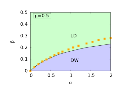
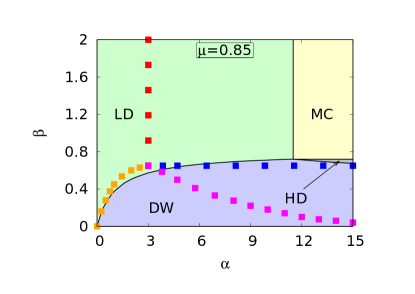
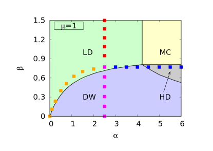
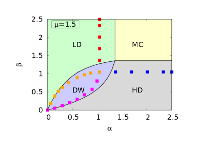
Figure 3: Phase diagrams in the weak coupling limit of the model are shown for different filling factors ($\mu$) with equal exchange rates ($k_{10}=k_{20}=0.95$). Depending on the value of $\mu$ which can be between 0 and $\mu_{\text{max}}=(2+k_{20}/k_{10})=3$, two or four distinct phases are observed simultaneously, using both MFT and MCS. These phases are LD, HD, MC, and DW, represented by green, gray, yellow, and blue regions respectively with solid black lines separting the phases, according to MFT; while MCS confirms the phase boundaries with discrete colored points: red (LD-MC), blue (HD-MC), orange (LD-DW), and magenta (HD-DW). Significant discrepancy between theoretical and simulated results are captured in the phase diagrams. With these equal exchange rates, phase diagrams for $\mu>3/2$ are related to those with $\mu<3/2$ by particle-hole symmetry, where $\mu=3/2$ is the half-filled limit; see Fig. 10.

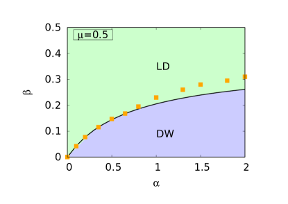
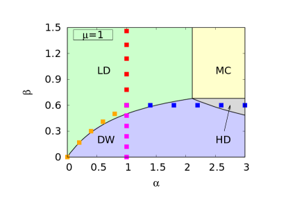
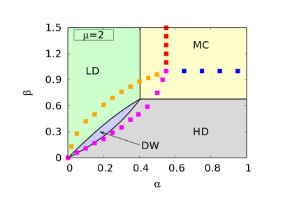
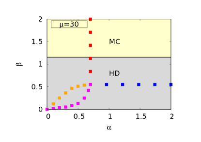
Figure 4: Phase diagrams in the weak coupling limit of the model are depicted for various filling factors ($\mu$) when exchange rates are $k_{10}=0.01$ and $k_{20}=0.95$. Again in this case, two or four distinct phases are observed subject to the particular value of $\mu$ which varies between 0 and $\mu_{\text{max}}=(2+k_{20}/k_{10})=97$. The phases LD, HD, MC, and DW are represented by green, gray, yellow, and blue regions respectively with solid black line as the phase boundaries, according to MFT and are compared to the MCS phase boundaries indicated by discrete colored points: red (LD-MC), blue (HD-MC), orange (LD-DW), and magenta (HD-DW). However, noticeable deviations between theoretical and simulated results are observed in the phase diagrams. Unlike Fig. 3, phase diagrams for the present unequal choice of exchange rates are not related by particle-hole symmetry.

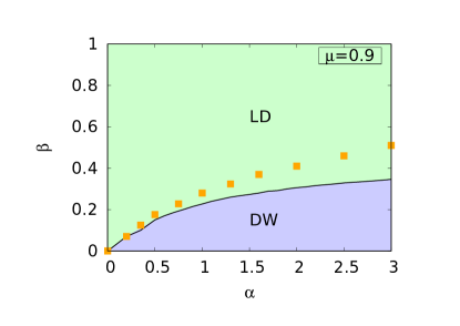
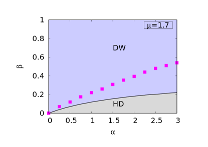
Figure 5: Phase diagrams in the weak coupling limit of the model are shown when exchange rates are $k_{10}=1$ and $k_{20}=0.1$. Background colors represent different phases and black solid lines are the boundaries separating them, according to MFT; wherein discrete colored points are the MCS phase boundaries. When $\mu=0.9$, only two phases, LD and DW, appear, and when $\mu=1.7$, the phases HD and DW occur. According to the condition in (47), for MC phase existence, the system’s $\mu_{\text{max}}$ should be greater than 3.75 with the chosen exchange rates $k_{10}$ and $k_{20}$, which is not satisfied in the present case where $\mu_{\text{max}}=(2+k_{20}/k_{10})=2.1$. Consistent with this MFT prediction, the MC phase is absent according to MCS also for any value of $\mu$ within 0 and 2.1. The MCS phase diagrams show qualitative similarities, but there are quantitative discrepancies compared to the MFT phase diagrams

Detailed quantitative analysis of the MFT phase diagrams are given below.

V STEADY STATE DENSITIES AND PHASE BOUNDARIES

V.1 Low-density phase

In the LD phase, the steady state density $\rho_{\text{LD}}$ is given by

$$\rho_{\text{LD}}=\alpha_{\text{eff}}=\alpha\frac{N_{1}}{L}<\frac{1}{2}.$$ (21)

Substituting $N_{1}$ from eq. (17a) in eq. (21) and identifying the steady current in LD phase as $J_{\text{LD}}=\rho_{\text{LD}}(1-\rho_{\text{LD}})$, one finds the following quadratic equation in $\rho_{\text{LD}}$:

$$\rho_{\text{LD}}=\alpha\bigg{[}\frac{k_{2}}{k_{1}+k_{2}}(\mu-\rho_{\text{LD}})-\frac{\rho_{\text{LD}}(1-\rho_{\text{LD}})}{L(k_{1}+k_{2})}\bigg{]},$$ (22)

which, in the weak coupling limit (where $k_{1(2)}=k_{10(20)}/L$), translates into

$$\rho_{\text{LD}}=\alpha\bigg{[}\frac{k_{20}}{k_{10}+k_{20}}(\mu-\rho_{\text{LD}})-\frac{\rho_{\text{LD}}(1-\rho_{\text{LD}})}{k_{10}+k_{20}}\bigg{]}.$$ (23)

Eq. (23) has two solutions:

$$\begin{split}\rho_{\text{LD}}^{\pm}&=\bigg{(}{\frac{1+k_{20}}{2}+\frac{k_{10}+k_{20}}{2\alpha}}\bigg{)}\\ &\quad\pm\bigg{[}\bigg{(}{\frac{1+k_{20}}{2}+\frac{k_{10}+k_{20}}{2\alpha}}\bigg{)}^{2}-\mu k_{20}\bigg{]}^{\frac{1}{2}}.\end{split}$$ (24)

When $\mu$ equals zero, the LD phase density must be zero. Therefore, out of the two solutions in (24), the physically acceptable solution is the one that vanishes as $\mu\rightarrow 0$, i.e., in the limit of vanishingly small number of particles. We thus get

$$\begin{split}\rho_{\text{LD}}&=\rho_{\text{LD}}^{-}\\ &=\bigg{(}{\frac{1+k_{20}}{2}+\frac{k_{10}+k_{20}}{2\alpha}}\bigg{)}-\\ &\quad\bigg{[}\bigg{(}{\frac{1+k_{20}}{2}+\frac{k_{10}+k_{20}}{2\alpha}}\bigg{)}^{2}-\mu k_{20}\bigg{]}^{\frac{1}{2}}\end{split}$$ (25)

as the solution for the LD phase density. Unsurprisingly, $\rho_{\text{LD}}$ as given in (25) is independent of $\beta$, the exit end rate parameter.

We can obtain from eq. (21) the expression of $N_{1}$; which is related to $N_{2}$ by the PNC equation, which reads $N_{0}=N_{1}+N_{2}+L\rho_{\text{LD}}$ in the LD phase. Thus, recalling $N_{0}=\mu L$ and the acceptable density in LD phase [eq. (25)], the expressions obtained for $N_{1}$ [using (21)] and $N_{2}$ (using PNC after obtaining $N_{1}$) are:

$$N_{1}=\frac{L}{\alpha}\rho_{\text{LD}},$$ (26)

$$N_{2}=L\bigg{(}\mu-\frac{1+\alpha}{\alpha}\rho_{\text{LD}}\bigg{)}.$$ (27)

As $\mu$ increases, more particles are available in the system and in the TASEP lane. Consequently, it is expected that for sufficiently high values of $\mu$, the TASEP lane will transition out of the LD phase. The range of $\mu$ over which the LD phase exists can be obtained from the condition $0<\rho_{\text{LD}}<1/2$, which is

$$0<\mu<\left(\frac{1}{2}+\frac{1}{4k_{20}}+\frac{k_{10}}{2\alpha k_{20}}+\frac{1}{2\alpha}\right).$$ (28)

This range indicates that the upper threshold of $\mu$ for the existence of the LD phase is a function of $\alpha$, $k_{10}$, and $k_{20}$. The upper threshold of $\mu$ in (28) is positive definite for positive parameters $\alpha$, $k_{10}$, and $k_{20}$, and can vary depending on their specific values. When this upper threshold is less than $\mu_{\text{max}}=(2+k_{20}/k_{10})$, i.e.,

$$\mu_{\text{max}}>\left(\frac{1}{2}+\frac{1}{4k_{20}}+\frac{k_{10}}{2\alpha k_{20}}+\frac{1}{2\alpha}\right),$$ (29)

beyond a certain threshold value of $\mu$, the LD phase ceases to exist due to an excess supply of particles. Conversely, when it equals $\mu_{\text{max}}$, the LD phase can persist for all values of $\mu$ ranging from 0 to $\mu_{\text{max}}$.

For the specific case of $k_{10}=k_{20}=0.95$, the range of $\mu$ over which the LD phase exists is $0<\mu<(0.76+1/\alpha)$. When considering $\mu=1$, the condition $\mu<(0.76+1/\alpha)$ indicates the occurrence of the LD phase for any $\alpha<4.17$ according to MFT. Similarly, for the case of $k_{10}=0.01$ and $k_{20}=0.95$, the range becomes $0<\mu<(0.76+0.505/\alpha)$, indicating the presence of the LD phase for any $\alpha<2.1$ when $\mu=1$. The phase diagrams in Fig. 3 and Fig. 4, which include both the MFT and MCS results on the phase diagrams, show the LD phase within these calculated ranges, while also highlighting deviations of the MCS results from MFT predictions. In Fig. 21, we present the LD phase density profiles in the weak coupling limit for $\mu=0.5$ and $\alpha=0.2,\,1$. The density profiles obtained from MCS agree well with the theoretical predictions of MFT for the lower $\alpha$ values. However, a quantitative discrepancy arises between the two for higher $\alpha$ values.

V.2 High-density phase

Next, we turn to the HD phase where the steady state bulk density is given by

$$\rho_{\text{HD}}=1-\beta_{\text{eff}}=1-\beta\bigg{(}1-\frac{N_{2}}{L}\bigg{)}>\frac{1}{2}.$$ (30)

Substitution of the expression of $N_{2}$ from eq. (17b) into eq. (30) leads to a quadratic equation in $\rho_{\text{HD}}$ given below:

$$\rho_{\text{HD}}=1-\beta+\beta\bigg{[}\frac{k_{1}}{k_{1}+k_{2}}(\mu-\rho_{\text{HD}})+\frac{\rho_{\text{HD}}(1-\rho_{\text{HD}})}{L(k_{1}+k_{2})}\bigg{]},$$ (31)

which, in the weak coupling limit, reads

$$\rho_{\text{HD}}=1-\beta+\beta\bigg{[}\frac{k_{10}}{k_{10}+k_{20}}(\mu-\rho_{\text{HD}})+\frac{\rho_{\text{HD}}(1-\rho_{\text{HD}})}{k_{10}+k_{20}}\bigg{]}.$$ (32)

Solving eq. (32) for $\rho_{\text{HD}}$ gives two solutions:

$$\begin{split}\rho_{\text{HD}}^{\pm}&=\bigg{(}\frac{1-k_{10}}{2}-\frac{k_{10}+k_{20}}{2\beta}\bigg{)}\pm\bigg{[}\bigg{(}\frac{1-k_{10}}{2}\\ &\quad-\frac{k_{10}+k_{20}}{2\beta}\bigg{)}^{2}+\mu k_{10}-\bigg{(}1-\frac{1}{\beta}\bigg{)}(k_{10}+k_{20})\bigg{]}^{\frac{1}{2}}.\end{split}$$ (33)

Between these two solutions, the physically acceptable one is the solution where the TASEP density reaches 1 at $\mu=\mu_{\text{max}}$. We thus get

$$\begin{split}\rho_{\text{HD}}&=\rho_{\text{HD}}^{+}\\ &=\bigg{(}\frac{1-k_{10}}{2}-\frac{k_{10}+k_{20}}{2\beta}\bigg{)}+\bigg{[}\bigg{(}\frac{1-k_{10}}{2}\\ &\quad-\frac{k_{10}+k_{20}}{2\beta}\bigg{)}^{2}+\mu k_{10}-\bigg{(}1-\frac{1}{\beta}\bigg{)}(k_{10}+k_{20})\bigg{]}^{\frac{1}{2}}\end{split}$$ (34)

as the acceptable HD phase density. The HD phase density, to no surprise, is independent of $\alpha$. Upon using (30) we derive the expression of $N_{2}$ in terms of $\rho_{\text{HD}}$, which is connected to $N_{1}$ by the PNC equation given by $N_{0}=N_{1}+N_{2}+L\rho_{\text{HD}}$ in the HD phase. Consequently, we determine the populations of the reservoirs, $N_{1}$ and $N_{2}$, as follows:

$$N_{1}=L\bigg{(}\mu-1+\frac{1}{\beta}-\frac{1+\beta}{\beta}\rho_{\text{HD}}\bigg{)},$$ (35)

$$N_{2}=L\bigg{(}1-\frac{1}{\beta}+\frac{\rho_{\text{HD}}}{\beta}\bigg{)}.$$ (36)

For the system to sustain the HD phase, an adequate supply of particles is necessary. In cases where the particle supply is insufficient, the HD phase is absent from the phase diagram. The range of $\mu$ that allows for the existence of the HD phase can be determined by considering $1/2<\rho_{\text{HD}}<1$. This provides us with the following range for $\mu$ over which the HD phase exists:

$$\left(\frac{3}{2}+\frac{k_{20}}{k_{10}}-\frac{1}{4k_{10}}-\frac{k_{20}}{2\beta k_{10}}-\frac{1}{2\beta}\right)<\mu<\bigg{(}2+\frac{k_{20}}{k_{10}}\bigg{)}.$$ (37)

As indicated in (37), the lower threshold of $\mu$ required for the existence of the HD phase is a function of $\beta$, $k_{10}$, and $k_{20}$. Depending on the values of $\beta$, $k_{10}$, and $k_{20}$, this lower threshold can either be positive or negative. When positive, the lower threshold implies a restricted $\mu$ value below which the HD phase is unobservable. In that case,

$$\left(\frac{3}{2}+\frac{k_{20}}{k_{10}}-\frac{1}{4k_{10}}-\frac{k_{20}}{2\beta k_{10}}-\frac{1}{2\beta}\right)>0$$

$$\implies \mu_{\text{max}}>\bigg{(}\frac{1}{2}+\frac{1}{4k_{10}}+\frac{k_{20}}{2\beta k_{10}}+\frac{1}{2\beta}\bigg{)}.$$ (38)

where $\mu_{\text{max}}=(2+k_{20}/k_{10})$. When it is zero or negative, the HD phase can be obtained for any value of $\mu$, however small it may be.

To illustrate with examples, let us consider the case where $k_{10}=k_{20}=0.95$. With these values of particle exchange rates, the required range of $\mu$ for the existence of the HD phase is $(2.24-1/\beta)<\mu<3$. When setting $\mu=1$, the HD phase is possible only for $\beta<0.88$, as depicted in the phase diagram of Fig. 3. In the second case where $k_{10}=0.01,k_{20}=0.95$, the range over which HD phase occurs is calculated as $(71.5-48/\beta)<\mu<97$. Clearly, when $\mu=1$, HD phase must appear in the region where $\beta<0.68$, which is consistent with Fig. 4. Fig. 21 shows the HD phase density profiles in the weak coupling limit for $\mu=2.5$ and two different values of $\beta$: $\beta=0.1$ and $\beta=1$. The MCS results agree well with the MFT predictions for the lower $\beta$ value, but deviate quantitatively for the higher $\beta$ value.

V.3 Maximal current phase

The MC phase is characterised by a steady state bulk density of $\rho_{\text{MC}}=1/2$ when homogeneous hopping with a rate of 1 occurs throughout the lattice bulk. The PNC relation then reads $N_{0}=N_{1}+N_{2}+L/2$ in the MC phase. Similar to the open TASEP, the MC phase in this model arises under the following conditions:

$$\alpha_{\text{eff}}=\alpha\frac{N_{1}}{L}>\frac{1}{2},$$ (39)

$$\beta_{\text{eff}}=\beta\bigg{(}1-\frac{N_{2}}{L}\bigg{)}>\frac{1}{2}.$$ (40)

As we will show in subsection V.5 below, the LD-MC and HD-MC boundaries are given by the conditions

$$\alpha=\frac{k_{10}+k_{20}}{(2\mu-1)k_{20}-\frac{1}{2}},$$ (41)

$$\beta=\frac{k_{10}+k_{20}}{(3-2\mu)k_{10}+2k_{20}-\frac{1}{2}},$$ (42)

respectively. The non-negativity of $\alpha$ and $\beta$, when considered in (41) and (42), demands the following two conditions on $\mu$:

$$\mu>\left(\frac{1}{2}+\frac{1}{4k_{20}}\right),$$ (43)

$$\mu<\left(\frac{3}{2}+\frac{k_{20}}{k_{10}}-\frac{1}{4k_{10}}\right)$$ (44)

respectively. We thus find the lower and upper thresholds of $\mu$ in (43) and (44) for MC phase existence. Taken together, the range of $\mu$ over which MC phase appears is as follows:

$$\left(\frac{1}{2}+\frac{1}{4k_{20}}\right)<\mu<\left(\frac{3}{2}+\frac{k_{20}}{k_{10}}-\frac{1}{4k_{10}}\right).$$ (45)

The fact that the lower and upper thresholds of $\mu$ for the MC phase to exist depend only on the particle exchange rates and not on the entrance and exit rate parameters implies that the occurrence of the MC phase is solely a bulk phenomenon and has no connection with the boundary conditions.

To ensure that the thresholds of $\mu$ obtained in (45) for MC phase existence is meaningful, the upper threshold must be greater than the lower threshold for any value of $k_{10}$ and $k_{20}$:

$$\left(\frac{3}{2}+\frac{k_{20}}{k_{10}}-\frac{1}{4k_{10}}\right)>\left(\frac{1}{2}+\frac{1}{4k_{20}}\right).$$ (46)

Simplifying this inequality, we obtain the following condition for the MC phase to occur:

$$\mu_{\text{max}}>\bigg{[}1+\frac{1}{4}\bigg{(}\frac{1}{k_{10}}+\frac{1}{k_{20}}\bigg{)}\bigg{]},$$ (47)

where $\mu_{\text{max}}$ is defined as $\mu_{\text{max}}=(2+k_{20}/k_{10})$.

In the special case where $k_{10}=k_{20}=k_{0}$, the range of $\mu$ over which MC phase comes into existence is determined by the condition (45), which translates as $(1/2+1/4k_{0})<\mu<(5/2-1/4k_{0})$, clearly demonstrating the particle-hole symmetry of the model with $\mu=3/2$ as the half-filled limit. We consider $k_{10}=k_{20}=0.95$, for which the range of $\mu$ for the existence of the MC phase becomes $0.76<\mu<2.24$ according to MFT. This is supported by MCS in Fig. 3, where no MC phase is observed at $\mu=0.5$. In the second case, where the exchange rates are highly asymmetric with $k_{10}=0.01$ and $k_{20}=0.95$, the MC phase exists within the range of $0.76<\mu<71.5$, according to MFT. Finally, in the third case when $k_{10}=1$ and $k_{20}=0.1$, MC phase does not exist as $\mu_{\text{max}}=(2+k_{20}/k_{10})=2.1$, inconsistent with the condition (47) which requires $\mu_{\text{max}}$ to be greater than 3.75 for this choice of $k_{10},\,k_{20}$; see Fig. 5. The condition for the existence of the MC phase in the limit of $k_{10}\rightarrow 0$ is determined by the upper limit of $\mu$ in (45), which can be expressed as $[3/2+1/k_{10}(k_{20}-1/4)]$. If $k_{20}$ is greater than 1/4, the MC phase exists due to the HD-MC boundary remaining on the positive side of the $\alpha$-axis. However, if $k_{20}$ is less than 1/4, the MC phase is absent. Therefore, the condition for the MC phase’s existence in the limit $k_{10}\rightarrow 0$ is governed by the requirement of $k_{20}>1/4$. Fig. 21 exhibits the MC phase density profile in the weak coupling limit for $\mu=1.5$ and $\alpha=\beta=2.5$.

V.4 Domain wall phase

In an open TASEP, the LD and HD phases meet when $\alpha_{T}=\beta_{T}<1/2$, or $\rho_{\text{LD}}+\rho_{\text{HD}}=1$, which is a straight line in the plane of the control parameters $\alpha_{T},\,\beta_{T}$, starting at (0,0) and terminating at (1/2,1/2). Precisely on this line, there is coexistence of the LD and HD phases in the form of a single delocalised domain wall (DDW) blythe . The delocalization is due to particle non-conserving dynamics.

In the present model, global particle number conservation ensures the ensuing domain wall to be confined at a specific location, say $x_{w}$, in the bulk of TASEP lane. We thus get a localised domain wall (LDW). The non-uniform spatial dependence of density in the DW phase can be represented as follows:

$$\rho(x)=\rho_{\text{LD}}+\Theta(x-x_{w})(\rho_{\text{HD}}-\rho_{\text{LD}}),$$ (48)

where $\Theta$ is the Heaviside step function defined as $\Theta(x)=1(0)$ for $x>(<)0$. In analogy with an open TASEP, the condition for the DW phase is as follows:

$$\rho_{\text{LD}}+\rho_{\text{HD}}=1,$$ (49)

which yields

$$\alpha_{\text{eff}}=\beta_{\text{eff}}$$ (50)

$$\implies \alpha\frac{N_{1}}{L}=\beta\bigg{(}1-\frac{N_{2}}{L}\bigg{)}$$ (51)

Below we obtain the exact location $x_{w}$ and height $\Delta$ of the LDW in terms of the control parameters.

In the DW phase, particle number in $T$ can be expressed as

$$N_{T}=L\int_{0}^{1}\rho(x)dx,$$ (52)

where a multiplicative factor $L$ is introduced in the right-hand side to rescale the integration limit of the position variable $x$. Using (48) and (51) in (52), we get:

$$N_{T}=L\bigg{[}\alpha\frac{N_{1}}{L}(2x_{w}-1)+1-x_{w}\bigg{]}.$$ (53)

Identifying the steady state TASEP current in the DW phase as $J_{T}=\rho_{\text{LD}}(1-\rho_{\text{LD}})$ or $J_{T}=\rho_{\text{HD}}(1-\rho_{\text{HD}})$ and substituting the expressions of $N_{T}$ [see eq. (53)] and $J_{T}$ in eq. (17a) together with PNC, we obtain the following two equations coupled in $N_{1}/L$ and $x_{w}$:

$$\frac{N_{1}}{L}\bigg{[}1-\frac{\alpha}{\beta}+\alpha(2x_{w}-1)\bigg{]}-x_{w}+1=\mu-1,$$ (54)

$$\begin{split}\frac{N_{1}}{L}&=\frac{k_{2}}{k_{1}+k_{2}}\bigg{[}\mu-\alpha\frac{N_{1}}{L}(2x_{w}-1)-1+x_{w}\bigg{]}\\ &\quad-\frac{1}{L(k_{1}+k_{2})}\alpha\frac{N_{1}}{L}\bigg{(}1-\alpha\frac{N_{1}}{L}\bigg{)}.\end{split}$$ (55)

While solving eqs. (54) and (55) for $N_{1}/L$ and $x_{w}$, we get a qudratic equation for $N_{1}/L$ with two solutions:

$$\begin{split}\bigg{(}\frac{N_{1}}{L}\bigg{)}^{\pm}&=\bigg{(}\frac{1}{2\alpha}+\frac{k_{10}}{2\alpha^{2}}+\frac{k_{20}}{2\alpha\beta}\bigg{)}\\ &\quad\pm\bigg{[}\bigg{(}\frac{1}{2\alpha}+\frac{k_{10}}{2\alpha^{2}}+\frac{k_{20}}{2\alpha\beta}\bigg{)}^{2}-\frac{k_{20}}{\alpha^{2}}\bigg{]}^{\frac{1}{2}}.\end{split}$$ (56)

The density in the LD part of the DW is thus

$$\rho_{\text{LD}}=\alpha\frac{N_{1}}{L}=\bigg{(}\frac{1}{2}+\frac{k_{10}}{2\alpha}+\frac{k_{20}}{2\beta}\bigg{)}\pm\\ \bigg{[}\bigg{(}\frac{1}{2}+\frac{k_{10}}{2\alpha}+\frac{k_{20}}{2\beta}\bigg{)}^{2}-k_{20}\bigg{]}^{\frac{1}{2}}.$$ (57)

At the boundary between the LD and the DW phases, MFT must predict identical (low) density in the bulk of $T$. We now argue that in (57) the solution with a negative discriminant is actually the physically acceptable solution. Equating the density in LD phase [eq. (25)] and density in the LD domain of DW phase [eq. (57) with negative discriminant], we obtain the LD-DW boundary as follows:

$$\bigg{(}{\frac{1+k_{20}}{2}+\frac{k_{10}+k_{20}}{2\alpha}}\bigg{)}$$

$$-\bigg{[}\bigg{(}{\frac{1+k_{20}}{2}+\frac{k_{10}+k_{20}}{2\alpha}}\bigg{)}^{2}-\mu k_{20}\bigg{]}^{\frac{1}{2}}$$

$$=\bigg{(}\frac{1}{2}+\frac{k_{10}}{2\alpha}+\frac{k_{20}}{2\beta}\bigg{)}-\bigg{[}\bigg{(}\frac{1}{2}+\frac{k_{10}}{2\alpha}+\frac{k_{20}}{2\beta}\bigg{)}^{2}-k_{20}\bigg{]}^{\frac{1}{2}}.$$ (58)

The LD-DW boundary equation (V.4) can be simplified further (detailed calculation is given in Appendix) after which it reduces to a form which we will obtain later in subsection V.5. We find

$$\frac{N_{1}}{L}\bigg{(}1+\alpha-\frac{\alpha}{\beta}\bigg{)}=\mu-1$$ (59)

as the LD-DW phase boundary, where $N_{1}/L$ is given by

$$\begin{split}\frac{N_{1}}{L}&=\bigg{(}\frac{1}{2\alpha}+\frac{k_{10}}{2\alpha^{2}}+\frac{k_{20}}{2\alpha\beta}\bigg{)}\\ &\quad-\bigg{[}\bigg{(}\frac{1}{2\alpha}+\frac{k_{10}}{2\alpha^{2}}+\frac{k_{20}}{2\alpha\beta}\bigg{)}^{2}-\frac{k_{20}}{\alpha^{2}}\bigg{]}^{\frac{1}{2}}.\end{split}$$ (60)

Therefore, the acceptable solution of $N_{1}/L$ is the one with a negative discriminant; see eq. (60). Next, the expression for $N_{2}$ can be obtained using eq. (51). One finds

$$\frac{N_{2}}{L} =1-\frac{\alpha}{\beta}\frac{N_{1}}{L}$$

$$=1-\bigg{(}\frac{1}{2\beta}+\frac{k_{10}}{2\alpha\beta}+\frac{k_{20}}{2\beta^{2}}\bigg{)}$$

$$\quad+\bigg{[}\bigg{(}\frac{1}{2\beta}+\frac{k_{10}}{2\alpha\beta}+\frac{k_{20}}{2\beta^{2}}\bigg{)}^{2}-\frac{k_{20}}{\beta^{2}}\bigg{]}^{\frac{1}{2}},$$ (61)

Once we obtain the expression for $N_{1}/L$ in eq. (60), the position $x_{w}$ of the domain wall can be obtained using eq. (54). We find:

$$x_{w}=\frac{\bigg{(}1-\alpha-\frac{\alpha}{\beta}\bigg{)}\frac{N_{1}}{L}-\mu+2}{1-2\alpha\frac{N_{1}}{L}}.$$ (62)

Having the expression of $N_{1}/L$, it is straightforward to obtain the low and high densities in the DW phase:

$$\rho_{\text{LD}} =\left(\frac{1}{2}+\frac{k_{10}}{2\alpha}+\frac{k_{20}}{2\beta}\right)-\left[\left(\frac{1}{2}+\frac{k_{10}}{2\alpha}+\frac{k_{20}}{2\beta}\right)^{2}-k_{20}\right]^{\frac{1}{2}},$$ (63)

together with $\rho_{\text{HD}}=1-\rho_{\text{LD}}$. Now defined as the density difference between high and low density parts, the height ($\Delta$) of the DW comes out to be

$$\Delta =\rho_{\text{HD}}-\rho_{\text{LD}}$$

$$=\bigg{[}\bigg{(}1+\frac{k_{10}}{\alpha}+\frac{k_{20}}{\beta}\bigg{)}^{2}-4k_{20}\bigg{]}^{\frac{1}{2}}-\bigg{(}\frac{k_{10}}{\alpha}+\frac{k_{20}}{\beta}\bigg{)}$$ (64)

The position $x_{w}$ of the DW in the system ranges from 0 to 1, corresponding to, respectively, the boundaries between the HD and DW phases, and LD and DW phases. Within the DW phase region, the condition $\alpha_{\text{eff}}=\alpha N_{1}/L<1/2$, or $(1-2\alpha N_{1}/L)>0$ must be followed. Consequently, for $x_{w}>0$ in eq. (62), we must have its numerator positive:

$$\bigg{[}\bigg{(}1-\alpha-\frac{\alpha}{\beta}\bigg{)}\frac{N_{1}}{L}-\mu+2\bigg{]}>0$$ (65)

$$\implies \mu<\bigg{[}\bigg{(}1-\alpha-\frac{\alpha}{\beta}\bigg{)}\frac{N_{1}}{L}+2\bigg{]}.$$ (66)

This sets the upper threshold of $\mu$ for DW phase existence. To determine the lower threshold of $\mu$, we consider the condition $x_{w}<1$ in eq. (62), leading to the following condition:

$$\mu>\bigg{[}\bigg{(}1+\alpha-\frac{\alpha}{\beta}\bigg{)}\frac{N_{1}}{L}+1\bigg{]}.$$ (67)

Hence, the range of $\mu$ over which the DW phase appears is

$$\bigg{[}\bigg{(}1+\alpha-\frac{\alpha}{\beta}\bigg{)}\frac{N_{1}}{L}+1\bigg{]}<\mu<\bigg{[}\bigg{(}1-\alpha-\frac{\alpha}{\beta}\bigg{)}\frac{N_{1}}{L}+2\bigg{]}.$$ (68)

Fig. 8 displays density profiles in the DW phase under the weak coupling limit. Increasing values of $\mu$, $\alpha$, and $\beta$ amplify the discrepancies between MFT and MCS, emphasizing the limitations of the mean-field approximation in capturing system behavior.

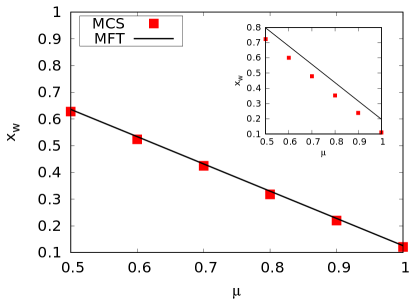
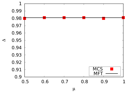
Figure 6: (Left) Plot of the domain wall position $x_{w}$ versus filling factor $\mu$ for a fixed value of exchange rates ($k_{10}=k_{20}=0.95$) in the weak coupling limit of the model. In the main plot, entry and exit rates are $\alpha=0.15$ and $\beta=0.01$, wherein corresponding values of those parameters in the inset plot is set to $\alpha=1$ and $\beta=0.1$. The location of the domain walls decreases linearly with increasing values of $\mu$. Reducing the values of $\alpha$ and $\beta$ improves the agreement between MFT and MCS results. (Right) Plot of the domain wall height $\Delta$ versus $\mu$ keeping $k_{10}=k_{20}=0.95$ in the weak coupling limit of the model with control parameters $\alpha=0.15$, $\beta=0.01$. The height of the domain wall $\Delta$ remains unchanged with varying $\mu$. Both the MFT and MCS results are in good agreement. Overall, the observed behavior suggests a repositioning of the domain walls towards the entrance end of the TASEP lane as the particle supply, represented by $\mu$, increases, without changing the domain wall height.

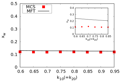
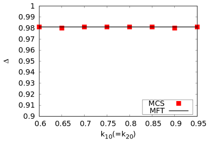
Figure 7: (Left) Plot of DW position $x_{w}$ vs. the exchange rates $k_{10}=k_{20}$ for a fixed value of filling factor ($\mu=1$) in the weak coupling limit of the model. The parameters used are $\alpha=0.15$, $\beta=0.01$ (main plot), and $\alpha=1$, $\beta=0.1$ (inset plot). Disagreement between the MFT and MCS results are reduced significantly for smaller values of $\alpha$, $\beta$. (Right) Plot of DW height $\Delta$ with respect to the exchange rates $k_{10}=k_{20}$ in the weak coupling limit of the model for a fixed value of $\mu$. The control parameters employed are $\alpha=0.15$, $\beta=0.01$, and $\mu=1$. For the specific values of the parameters employed, the DW position and height remain unchanged with the variation of exchange rates within the noted range.

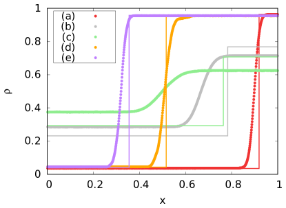
Figure 8: Plots illustrating the density $\rho$ as a function of position $x$ in the DW phase under the weak coupling limit. The solid lines correspond to the theoretical predictions from mean-field theory (MFT), while the data points obtained from Monte Carlo simulations (MCS) share the same color as their respective mean-field counterparts. The parameter values used are mentioned herein: (a) $\alpha=0.2$, $\beta=0.045$, $\mu=0.5$, $k_{10}=k_{20}=0.95$; (b) $\alpha=1$, $\beta=0.4$, $\mu=1$, $k_{10}=k_{20}=0.95$; (c) $\alpha=1.5$, $\beta=0.5$, $\mu=1$, $k_{10}=k_{20}=0.95$; (d) $\alpha=0.1$, $\beta=0.07$, $\mu=1.3$, $k_{10}=0.7$, $k_{20}=0.9$; and (e) $\alpha=0.2$, $\beta=0.05$, $\mu=1$, $k_{10}=0.4$, $k_{20}=0.8$.

We now consider how the DW location $x_{w}$ and its height $\Delta$ depend upon $\mu$. Our MF value of $x_{w}$, as given in (62), gives a linear decrease in $x_{w}$ with increasing $\mu$, while keeping other control parameters, such as $\alpha$, $\beta$, and $k_{10(20)}$, unchanged. Further in the MFT, eq. (64) shows that $\Delta$ remains independent of $\mu$. Thus, if there is a higher supply of particles into the TASEP lane, as would happen with a higher $\mu$, the DW position will move towards the entry end, leaving its height unchanged, to accommodate the additional particles. These MFT predictions are consistent with our results from the MCS studies; Fig. 6.

Additionally, the relationship between the position or height of the domain wall and the exchange rate parameters $k_{10}$ and $k_{20}$, as given by eqs. (62) and (64), are illustrated in Fig. 7, where the behavior of LDW position and height assuming equal values for $k_{10}$ and $k_{20}$ are shown. Notably, under these specific conditions, the LDW position and height appear to be quite insensitive to the variations in the exchange rates.

V.5 Phase boundaries

Having obtained the steady state densities in different phases, the next task is to determine the phase boundaries. We first consider the LD-MC and HD-MC phase boundaries. Using the condition that at the boundary between the LD and MC phases, $\rho_{\text{LD}}=1/2$, and at the boundary between the HD and MC phases, $\rho_{\text{HD}}=1/2$, the LD-MC and HD-MC phase boundaries may be obtained by setting $\rho_{\text{LD}}=1/2$ and $\rho_{\text{HD}}=1/2$ in eqs. (25) and (34) respectively. We find

$$\alpha=\frac{k_{10}+k_{20}}{(2\mu-1)k_{20}-\frac{1}{2}},$$ (69)

$$\beta=\frac{k_{10}+k_{20}}{(3-2\mu)k_{10}+2k_{20}-\frac{1}{2}}$$ (70)

respectively, as the LD-MC and HD-MC phase boundaries, which are just straight lines parallel to $\beta$- and $\alpha$-axes, respectively, in the $\alpha-\beta$ plane; see Fig. 3 and Fig. 4.

We now discuss the boundaries of the DW phase with the LD and HD phases. When transitioning from the LD phase to the DW phase, the domain wall should be located at the extreme right end or the exit end of the TASEP lane. Similarly, at the transition from HD to DW phase, one finds the DW to be at the extreme left end or the entrance end. One thus sets $x_{w}=1$ in eq. (62) to obtain the LD-DW phase boundary:

$$\frac{N_{1}}{L}\bigg{(}1+\alpha-\frac{\alpha}{\beta}\bigg{)}=\mu-1,$$ (71)

and $x_{w}=0$ to obtain the HD-DW phase boundary:

$$\frac{N_{1}}{L}\bigg{(}1-\alpha-\frac{\alpha}{\beta}\bigg{)}=\mu-2,$$ (72)

where $N_{1}/L$ is given in eq. (60).

V.5.1 Phase boundaries meet at a common point

Phase diagrams in Fig. 3 and Fig. 4 reveal the four phases — LD, HD, MC, and DW — to meet at a single point named as the multicritical point. This unique point is represented by the coordinates $(\alpha_{\text{c}},\beta_{\text{c}})$ in the $\alpha-\beta$ plane:

$$(\alpha_{\text{c}},\beta_{\text{c}})=\bigg{(}\frac{k_{10}+k_{20}}{(2\mu-1)k_{20}-\frac{1}{2}},\frac{k_{10}+k_{20}}{(3-2\mu)k_{10}+2k_{20}-\frac{1}{2}}\bigg{)}.$$ (73)

By definition, $\alpha_{\text{c}}$ and $\beta_{\text{c}}$ must be positive which puts the multicritical point within the first quadrant of the $\alpha-\beta$ phase diagram. This implies the following range of $\mu$ within which multicritical point exists:

$$\bigg{(}\frac{1}{2}+\frac{1}{4k_{20}}\bigg{)}<\mu<\bigg{(}\frac{3}{2}+\frac{k_{20}}{k_{10}}-\frac{1}{4k_{10}}\bigg{)}.$$ (74)

Apparent from (74), the lower and upper thresholds of $\mu$ for the existence of a multicritical point depend only on the exchange rates $k_{10}$ and $k_{20}$. That the upper threshold in (74) is greater than the lower threshold gives the condition

$$\mu_{\text{max}}>\left[1+\frac{1}{4}\left(\frac{1}{k_{10}}+\frac{1}{k_{20}}\right)\right].$$ (75)

This condition (75) is consistent with the condition (47) for the existence of MC phase, derived earlier.

The distance $d$ between the origin $(0,0)$ and the multicritical point $(\alpha_{\text{c}},\beta_{\text{c}})$ is

$$d=\sqrt{\bigg{(}\frac{k_{10}+k_{20}}{(2\mu-1)k_{20}-\frac{1}{2}}\bigg{)}^{2}+\bigg{(}\frac{k_{10}+k_{20}}{(3-2\mu)k_{10}+2k_{20}-\frac{1}{2}}\bigg{)}^{2}}.$$ (76)

Fig. 9 shows the variation of $d$ with $\mu$ according to MFT and MCS. It is important to note that the value of $d$ diverges as $\mu$ approaches $(1/2+1/4k_{20})$ from above and $(3/2+k_{20}/k_{10}-1/4k_{10})$ from below. Thus, when $k_{10}=k_{20}=0.95$, $d$ diverges when $\mu$ goes to 0.76 from above or 2.24 from below according to MFT prediction. The MCS plot, however, shows these divergences in $d$ at a shifted value of $\mu$ from the theoretical predictions.

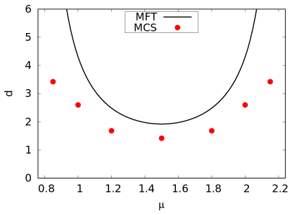
Figure 9: Plot of the distance $d$ between the origin and the multicritical point versus filling factor $\mu$ in the weak coupling limit of the model. Particle exchage rates between reservoirs are taken to be same, i.e., $k_{10}=k_{20}=0.95$. Black solid line and colored discrete points represent the MFT and MCS results respectively. Despite matching qualitatively, there is a quantitative discrepancy between the results from MFT and MCS.

VI PARTICLE-HOLE SYMMETRY AND THE PHASE DIAGRAMS WITH EQUAL EXCHANGE RATES ($\mathbf{k_{10}=k_{20}}$)

We consider the case where the particle exchange rates are same in magnitude, i.e., $k_{10}=k_{20}$, for which there is a particle-hole symmetry. The LD-MC phase boundary is interchanged with the HD-MC phase boundary, and the LD-DW phase boundary is interchanged with the HD-DW phase boundary, under the transformations $\mu\leftrightarrow 3-\mu$ and $\alpha\leftrightarrow\beta$; see eqs. (69), (70), (71), and (72). This symmetry around the half-filled limit ($\mu=3/2$) demonstrates the presence of particle-hole symmetry in the phase diagrams. The particle-hole symmetry can also be expressed in terms of the steady state densities in the LD and HD phases for equal exchange rates. One finds the correlation $\rho_{\text{LD}}\leftrightarrow 1-\rho_{\text{HD}}$; see eqs. (25) and (34) underlying. In Fig. 10, we present the phase diagram for $\mu=2$ which is connected to the phase diagram for $\mu=1$ shown in Fig. 3 by this symmetry. However, the symmetry breaks when unequal exchange rates are considered (cf. Fig. 4).

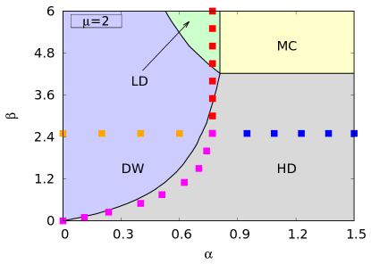
Figure 10: Phase diagram in the weak coupling limit of the model for $\mu=2$, with equal exchange rates $k_{10}=k_{20}=0.95$. Notably, this phase diagram exhibits a particle-hole symmetry with the phase diagram corresponding to $\mu=1$ in Fig. 3. All four phases are obtained for this choice of $\mu$. The background colors in the diagram represent different phases, while the black solid lines indicate the boundaries between those phases according to mean-field theory (MFT). To validate these boundaries, MCS results are included in the form of colored discrete points representing the phase boundaries.

VII NATURE OF THE PHASE TRANSITIONS

The phases in the phase diagrams in Fig. 3, Fig. 4, and Fig. 5 are demarcated by different phase boundaries. We will now discuss the nature of the transitions across these phase boundaries. In a TASEP with open boundaries, with the bulk density $\rho$ as the order parameter, the transition between the LD and HD phases is accompanied by a sudden jump in $\rho$, implying thus a discontinuous or first-order transition. Similarly, the transitions between either LD or HD and MC phases are continuous or second-order transitions, with the density difference vanishing smoothly across the phase boundaries. The transitions in the present model can be described in terms of the densities in the TASEP lane $T$ and can be classified in analogy with open TASEP by noting the density changes (sudden jump or smooth). In the present model, all the phase transitions – LD-DW, HD-DW, LD-MC, and HD-MC – are continuous in nature, as the density changes continuously and smoothly across all of them. In Fig. 3, the phase diagram corresponding to $\mu=0.5$ exhibits only one second-order phase transition (LD-DW), whereas phase diagrams with other values of $\mu$ include all four second-order phase transitions (LD-DW, HD-DW, LD-MC, and HD-MC), according to MFT and MCS both. Next in Fig. 4, the phase diagram for $\mu=0.5$ shows one continuous phase transition (LD-DW), while for $\mu=1$ and $\mu=2$, all four continuous phase transitions are present, as predicted by both MFT and MCS. Interestingly, the phase diagram corresponding to $\mu=30$ exhibits one continuous phase transition (HD-MC) according to MFT but includes all four continuous phase transitions according to MCS. Lastly, in Fig. 5, phase diagram associated with $\mu=0.9$ and $\mu=1.7$ contains one continuous phase transition, LD-DW and HD-DW respectively, according to both MFT and MCS. For some ranges of $\mu$, there can be all the four phases which meet at a common point; see Fig. 3 and Fig. 4. This common meeting point is then a multicritical point.

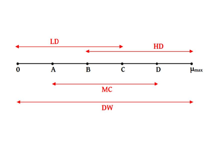
Figure 11: A schematic representation illustrating the ranges of $\mu$ where various phases emerge in the weak coupling limit of the model.

In Fig. 11, occurrence of different phases within a specific range of $\mu$ is tangible. Following are the expressions corresponding to the points on the $\mu$ axis.

• A: $\bigg{(}\frac{1}{2}+\frac{1}{4k_{20}}\bigg{)}$

• B: $\bigg{(}\frac{3}{2}+\frac{k_{20}}{k_{10}}-\frac{1}{4k_{10}}-\frac{k_{20}}{2\beta k_{10}}-\frac{1}{2\beta}\bigg{)}$

• C: $\bigg{(}\frac{1}{2}+\frac{1}{4k_{20}}+\frac{k_{10}}{2\alpha k_{20}}+\frac{1}{2\alpha}\bigg{)}$

• D: $\bigg{(}\frac{3}{2}+\frac{k_{20}}{k_{10}}-\frac{1}{4k_{10}}\bigg{)}$

• $\mathbf{\mu_{\text{max}}}=\bigg{(}2+\frac{k_{20}}{k_{10}}\bigg{)}$

These points are the thresholds of $\mu$ for the existence of different phases as obtained in (28), (37), and (45). We restate below the conditions (29), (38), and (47), which $\mu_{\text{max}}$ satisfies.

$$\mu_{\text{max}}>\bigg{(}\frac{1}{2}+\frac{1}{4k_{20}}+\frac{k_{10}}{2\alpha k_{20}}+\frac{1}{2\alpha}\bigg{)},$$ (77)

$$\mu_{\text{max}}>\bigg{(}\frac{1}{2}+\frac{1}{4k_{10}}+\frac{k_{20}}{2\beta k_{10}}+\frac{1}{2\beta}\bigg{)},$$ (78)

$$\mu_{\text{max}}>\bigg{[}1+\frac{1}{4}\bigg{(}\frac{1}{k_{10}}+\frac{1}{k_{20}}\bigg{)}\bigg{]}.$$ (79)

It can be seen that C $\geq$ A and B $\leq$ D for any (positive) values of $\alpha$, $\beta$, $k_{10}$, and $k_{20}$. The points B and C, in addition to being dependent on the parameters $k_{10}$ and $k_{20}$, also vary with the values of $\alpha$ and $\beta$. This means that by adjusting $\alpha$ and $\beta$ while $k_{10}$ and $k_{20}$ kept fixed, we can move these points along the $\mu$-axis.

The point C is set to the right side of the point B. When C $\geq$ B, the following condition emerges:

$$\mu_{\text{max}}\leq\bigg{[}1+\frac{1}{4}\bigg{(}\frac{1}{k_{10}}+\frac{1}{k_{20}}\bigg{)}+\frac{1}{2\alpha}\bigg{(}1+\frac{k_{10}}{k_{20}}\bigg{)}+\frac{1}{2\beta}\bigg{(}1+\frac{k_{20}}{k_{10}}\bigg{)}\bigg{]}.$$ (80)

For certain positive values of the control parameters $\alpha$, $\beta$, $k_{10}$, and $k_{20}$, the condition (80) can go with the conditions (77), (78), and (79). The possibility, C $<$ B, is defied as it leads to the condition:

$$\mu_{\text{max}}>\bigg{[}1+\frac{1}{4}\bigg{(}\frac{1}{k_{10}}+\frac{1}{k_{20}}\bigg{)}+\frac{1}{2\alpha}\bigg{(}1+\frac{k_{10}}{k_{20}}\bigg{)}+\frac{1}{2\beta}\bigg{(}1+\frac{k_{20}}{k_{10}}\bigg{)}\bigg{]},$$ (81)

which may or may not align with the conditions (77), (78), and (79). Thus, the point C can position itself only on the right side of point B or coincide with it, but cannot be at the left side of B.

Now, let us explore how far the point C (or B) can be moved on the right (or left) side along the $\mu$-axis. Specifically, can point C be placed to the right of point D, or can point B be located to the left of point A? To help answer it, we, upon examining the expressions for points C and D, deduce that when C is positioned to the left of D, following condition for $\alpha$ has to be fulfilled:

$$\alpha>\frac{\bigg{(}1+\frac{k_{10}}{k_{20}}\bigg{)}}{2\bigg{[}1+\frac{k_{20}}{k_{10}}-\frac{1}{4}\bigg{(}\frac{1}{k_{10}}+\frac{1}{k_{20}}\bigg{)}\bigg{]}}.$$ (82)

Moreover, to ensure the occurrence of the HD and MC phases, the corresponding boundary equation (70) requires $\beta$ to be positive, which is fulfilled when $\mu<$ D. Now, at the boundary between LD and MC phases, $\alpha$ is given by (69), substituting which in (82) we get $\mu<$ D. If we consider positioning the point C on the right side of point D, it will lead to the condition:

$$\alpha<\frac{\bigg{(}1+\frac{k_{10}}{k_{20}}\bigg{)}}{2\bigg{[}1+\frac{k_{20}}{k_{10}}-\frac{1}{4}\bigg{(}\frac{1}{k_{10}}+\frac{1}{k_{20}}\bigg{)}\bigg{]}},$$ (83)

which corresponds to $\mu>$ D, or to put in other way, $\beta<0$. This is unphysical. These considerations restrict the location of point C in between the points A and D. In a way similar to what is done considering the points C and D, we can also conclude the location of point B to be constrained between the points A and D.

In summary, keeping the exchange rates $k_{10}$ and $k_{20}$ fixed, the positions of points A, D, and $\mu_{\text{max}}$ remain unchanged along the $\mu$-axis. On the other hand, points B and C have the flexibility to slide between A and D by tuning the values of $\alpha$ and $\beta$, with the constraint that C cannot be positioned to the left of B.

A comprehensive summary of the different phases, domain walls, phase boundaries, and multicritical points can be found in Table 1.

Row no.	Range of $\mu$	Phases	Domain walls	Phase boundaries	Multicritical points (MCPs)
1	$0<\mu<\bigg{(}\frac{1}{2}+\frac{1}{4k_{20}}\bigg{)}$	LD and DW	One LDW	One second-order	None
2	$\bigg{(}\frac{1}{2}+\frac{1}{4k_{20}}\bigg{)}<\mu<\bigg{(}\frac{3}{2}+\frac{k_{20}}{k_{10}}-\frac{1}{4k_{10}}-\frac{k_{20}}{2\beta k_{10}}-\frac{1}{2\beta}\bigg{)}$	LD, HD, MC, and DW	One LDW	Four second-order	One four-phase MCP
3	$\bigg{(}\frac{3}{2}+\frac{k_{20}}{k_{10}}-\frac{1}{4k_{10}}-\frac{k_{20}}{2\beta k_{10}}-\frac{1}{2\beta}\bigg{)}<\mu<\bigg{(}\frac{1}{2}+\frac{1}{4k_{20}}+\frac{k_{10}}{2\alpha k_{20}}+\frac{1}{2\alpha}\bigg{)}$	LD, HD, MC, and DW	One LDW	Four second-order	One four-phase MCP
4	$\bigg{(}\frac{1}{2}+\frac{1}{4k_{20}}+\frac{k_{10}}{2\alpha k_{20}}+\frac{1}{2\alpha}\bigg{)}<\mu<\bigg{(}\frac{3}{2}+\frac{k_{20}}{k_{10}}-\frac{1}{4k_{10}}\bigg{)}$	LD, HD, MC, and DW	One LDW	Four second-order	One four-phase MCP
5	$\bigg{(}\frac{3}{2}+\frac{k_{20}}{k_{10}}-\frac{1}{4k_{10}}\bigg{)}<\mu<(2+\frac{k_{20}}{k_{10}})$	HD and DW	One LDW	One second-order	None

Table 1: Table summarizing the occurence of certain phases and phase boundaries over a range of filling factor $\mu$ according to MFT in the weak coupling limit case. Particle-hole symmetry becomes relevant when a symmetric choice of exchange rates is considered, meaning $k_{10}=k_{20}$.

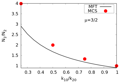
Figure 12: (Left) Variation of the reservoir population ratio $N_{1}/N_{2}$ with the filling factor $\mu$ for fixed values of the exchange rates $k_{10}=k_{20}=0.95$ in the weak coupling limit of the model. (Right) Variation of the reservoir population ratio $N_{1}/N_{2}$ with the exchange rate ratio $k_{10}/k_{20}$ for a fixed $\mu=3/2$ in the weak coupling limit. For both plots, the entry and exit rates are chosen such that the TASEP lane always remains in the LD phase. The values of $\alpha=0.1$ and $\beta=1$ are used. There is a slight mismatch between the results obtained from MFT and MCS in the left plot. However, in the right plot, the mismatch between MFT and MCS increases with decreasing exchange rate ratio.

VIII CONCLUSION AND OUTLOOK

In this article, we have studied how the interplay between the finite availability and carrying capacity of particles at different parts of a spatially extended system, and diffusion between these parts can control the steady state currents and steady state density profiles in a quasi-1D current-carrying channel connecting the different parts of the system. To address this issue, we propose and study a conceptual model that is composed of two reservoirs $R_{1}$ and $R_{2}$ of finite capacities and connected by a single TASEP channel at its entry and exit ends respectively. The reservoirs are allowed to exchange particles among them instantaneously, which models particle diffusion between them. The latter process ensures that there is a finite steady state current in the system. The model has five free parameters — the two parameters $\alpha,\beta$ defining the entry and exit rates, the two rates $k_{1},k_{2}$ for the particle exchanges between the reservoirs, and the filling fraction $\mu$. In addition, there are two functions, $f$ and $g$, that control the effective entry and exit rates, respectively. To simplify the subsequent analysis, we have chosen very simple forms for the functions $f$ and $g$, such that reservoir $R_{2}$ has a maximum capacity of $L$ particles, wheres reservoir $R_{1}$ has a capacity $k_{2}L/k_{1}$, where $L$ is the size of the TASEP channel. When $k_{1}=k_{2}$, the model admits a particle-hole symmetry, which is absent for $k_{1}\neq k_{2}$. We have used simple MFT and MCS to obtain the phase diagrams in the $\alpha-\beta$ plane and also the steady state density profiles, parametrised by all the other parameters. We have chosen $f$ to be monotonically rising, whereas $g$ is monotonically decreasing. We have studied our model in two distinct limits, when the particle exchange process competes with the TASEP current, and when it overwhelms the latter. We call the former weak coupling limit and the latter strong coupling limit of the model. Nonetheless, the model displays unexpected phase behavior not generally observed in the existing models for TASEPs with finite resources. First and foremost, depending upon the values of $\mu$, the model can either be in two or four phases, with continuous transitions between them. We have identified different threshold values of $\mu$ for the existence of the various phases. Secondly, the occupations $N_{1}$ and $N_{2}$ of the two reservoirs $R_{1}$ and $R_{2}$ are generally unequal. In fact, the populations of the two reservoirs could be preferentially controlled, i.e., getting them relatively populated or depopulated, by appropriate choice of the above model parameters. This in turn can lead to possible population imbalances in the steady states and consequently highly inhomogeneous particle distributions between different parts of the systems.

We have used analytical mean-field theory together with stochastic Monte Carlo simulations studies for our work. The mean-field theory predictions agree quantitatively with the corresponding MCS results in the strong coupling limit, but we find significant quantitative mismatch between the two in the weak coupling limit. We attribute this stronger fluctuations in the weak coupling limit of the model. In that limit, the ratio of the two reservoir populations $N_{1}$ and $N_{2}$ involves the TASEP current, and hence can fluctuate individually, affecting $\alpha_{\text{eff}}$ and $\beta_{\text{eff}}$ individually. In contrast, in the strong coupling limit, this ratio is a strict constant in the thermodynamic limit, and hence $\alpha_{\text{eff}}$ and $\beta_{\text{eff}}$ do not fluctuate independent of each other, but must maintain a definite relation. This suppresses the effects of fluctuations in the strong coupling limit. Our results have been obtained with specific choices for $f$ and $g$. While other choices for $f$ and $g$ should quantitatively change the phase diagram, so long as $f$ and $g$ remain monotonically increasing and decreasing functions of their arguments, and allow for maximum finite capacities of the reservoirs, we expect our results should hold qualitatively.

We have studied the simplest case with only one TASEP channel connecting two reservoirs. One can consider more than one TASEP channels and more than two reservoirs with diffusion between them. Our MFT can be in principle extended to such a system, whose precise mathematical form will of course depend upon the actual connectivity of the TASEP channels and the reservoirs. In such a situation, it is expected that the system may display more than one delocalised domain walls, one each in each channel, instead of a single LDW as here, for some choices of the model parameters. Stochastic simulations should be helpful to validate these qualitative expectations.

IX Acknowledgement

AB thanks SERB (DST), India for partial financial support through the CRG scheme [file: CRG/2021/001875].

Appendix A Details on the LD-DW phase boundary in the weak coupling case

Here we show explicitly how eq. (V.4) reduces to eq. (59). Denoting $a=\bigg{(}{\frac{1+k_{20}}{2}+\frac{k_{10}+k_{20}}{2\alpha}}\bigg{)}$ and $b=\bigg{(}\frac{1}{2}+\frac{k_{10}}{2\alpha}+\frac{k_{20}}{2\beta}\bigg{)}$, we rewrite eq. (V.4):

$$a-\sqrt{a^{2}-\mu k_{20}}=b-\sqrt{b^{2}-k_{20}}$$

$$\implies \frac{4}{k_{20}}[(\mu+1)ab-a^{2}-\mu b^{2}]=(\mu-1)^{2}.$$ (84)

Having the definition of $a$ and $b$, we compute the term inside the square bracket in eq. (84). With that being done, the resulting equation can be expressed as a quadratic equation in $\mu$ as follows:

$$\mu^{2}-\mu\bigg{(}3+\frac{1+k_{10}}{\alpha}-\frac{1-k_{20}}{\beta}+\frac{k_{10}}{\alpha^{2}}-\frac{k_{20}}{\beta^{2}}-\frac{k_{10}-k_{20}}{\alpha\beta}\bigg{)}$$

$$+2+k_{20}+\frac{1+k_{10}+2k_{20}}{\alpha}-\frac{1+k_{20}}{\beta}$$

$$+(k_{10}+k_{20})\bigg{(}\frac{1}{\alpha^{2}}-\frac{1}{\alpha\beta}\bigg{)}=0.$$ (85)

Next, defining $c=\bigg{(}\frac{1}{2}+\frac{k_{10}}{2\alpha}+\frac{k_{20}}{2\beta}\bigg{)}$, we recast eq. (59) as

$$\bigg{(}c-\sqrt{c^{2}-k_{20}}\bigg{)}\bigg{(}1+\frac{1}{\alpha}-\frac{1}{\beta}\bigg{)}=\mu-1$$

$$\implies c^{2}-k_{20}=\bigg{(}c-\frac{\mu-1}{1+\frac{1}{\alpha}-\frac{1}{\beta}}\bigg{)}^{2}$$

$$\implies \bigg{[}2c\bigg{(}1+\frac{1}{\alpha}-\frac{1}{\beta}\bigg{)}-\mu+1\bigg{]}(\mu-1)=k_{20}\bigg{(}1+\frac{1}{\alpha}-\frac{1}{\beta}\bigg{)}^{2}.$$ (86)

Again, with defined $c$, we compute the term inside the square bracket in eq. (86). Then, after some rearrangement of terms, the resulting equation can be seen as a quadratic equation in $\mu$ identical with eq. (85).

Appendix B STRONG COUPLING LIMIT

In this Section, we consider the strong coupling limit of the model, i.e., when $k_{1},\,k_{2}\sim{\cal O}(1)$ and independent of $L$. We shall see below that in this limit the direct particle exchanges between the reservoirs dominate. Therefore in the strong coupling limit, the particle numbers in the two reservoirs $R_{1}$ and $R_{2}$ maintain a fixed ratio for a given set of particle exchange rates (see below). This makes the ensuing MFT algebraically simpler and shows good agreement with the corresponding MCS studies results, in contrast to the weak coupling limit of the model. We set up the MFT following the logic used to develop the MFT in the weak coupling limit.

B.1 Mean-field phase diagrams and steady state densities

For specificity, we consider two cases, one with equal exchange rates $k_{1}=k_{2}=0.95$ with $\mu_{\text{max}}=3$, another with unequal exchange rates $k_{1}=0.01,k_{2}=0.95$ with $\mu_{\text{max}}=97$. The phase diagrams are shown in Fig. 13 and Fig. 14, respectively.

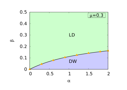
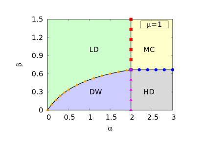
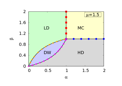
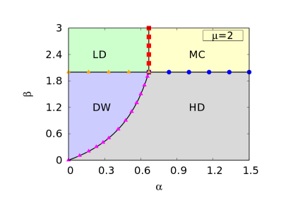
Figure 13: Phase diagrams of the model in the strong coupling limit for different $\mu$ with equal diffusion rates ($k_{1}=k_{2}=0.95$) are shown. Different colors in the background represents the region covered by distinct phases according to MFT which are seperated by black solid lines. To corroborate them, MCS phase boundaries in the form of discrete colored points are shown. Both are in excellent agreement. Depending on the specific value of $\mu$ which varies from 0 to $\mu_{\text{max}}=(2+k_{2}/k_{1})=3$, the phase diagrams contains either two or four distinct phases. With these equal exchange rates, particle-hole symmetry connects the phase diagrams for $\mu>3/2$ with the ones for $\mu<3/2$, $\mu=3/2$ being the half-filled limit.

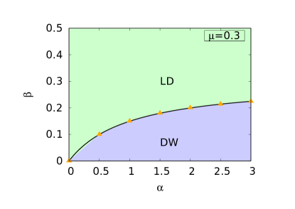
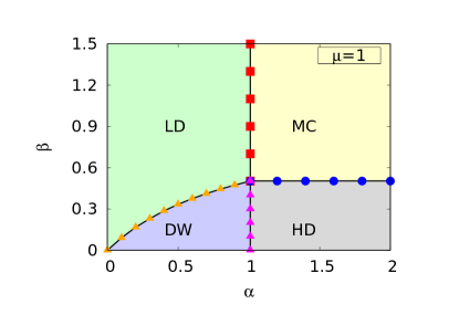
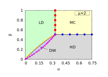
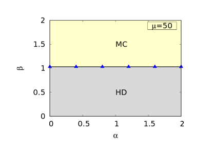
Figure 14: Phase diagrams of the model in the strong coupling limit for different $\mu$ with unequal diffusion rates ($k_{1}=0.01,k_{2}=0.95$) are shown. The background colors indicate distinct phases according to MFT, wherein the discrete colored points are the phase boundaries obtained by MCS. They are in good agreement with each other. The maximum value of $\mu$ in this case is calculated as $\mu_{\text{max}}=(2+k_{2}/k_{1})=97$. Unlike the phase diagrams obtained in Fig. 13, the phase diagrams in this case are not connected by any symmetry operation. This is attributed to the unequal exchange rates. When considering a significantly large value of $\mu$, such as $\mu=50$, only two phases, namely HD and MC, are tangible.

We start with the MFT eqs. (13) and (16) given above. As explained in Section III above, in the strong coupling limit

$$\frac{N_{2}}{N_{1}}=\frac{k_{1}}{k_{2}}$$ (87)

with $L\rightarrow\infty$. This considerably simplifies the MFT as discussed below in details.

B.1.1 Low-density phase

We proceed as in the weak coupling case. In the limit $L\rightarrow\infty$, the last term in the right-hand side of eq. (22) with the order of $\sim\mathcal{O}(1/L)$ vanishes and $\rho_{\text{LD}}$ can be approximated as a function of the TASEP parameters $\alpha$, $\mu$, $k_{1}$, and $k_{2}$ as following:

$$\rho_{\text{LD}}\approx\frac{\alpha k_{2}\mu}{k_{1}+(1+\alpha)k_{2}}.$$ (88)

Eq. (88) gives a linear dependence of $\rho_{\text{LD}}$ on $\mu$ with $\rho_{\text{LD}}=0$ when $\mu=0$. The form of $\rho_{\text{LD}}$ in eq. (88) allows for expressions to be obtained for the population of the two reservoirs:

$$N_{1}=\frac{Lk_{2}\mu}{k_{1}+(1+\alpha)k_{2}},$$ (89)

$$N_{2}=\frac{Lk_{1}\mu}{k_{1}+(1+\alpha)k_{2}}.$$ (90)

As mentioned above, the relative population of the two reservoirs becomes $N_{1}/N_{2}=k_{2}/k_{1}$, independent of other control parameters $\alpha$, $\beta$, and $\mu$.

With rising $\mu$, the availability of particles in the system, and hence to the TASEP lane, increases, and eventually, for high enough $\mu$, LD phase disappears. By definition, $0<\rho_{\text{LD}}<1/2$, we get the following range of $\mu$ over which LD phase appears:

$$0<\mu<\bigg{(}\frac{1}{2}+\frac{k_{1}}{2\alpha k_{2}}+\frac{1}{2\alpha}\bigg{)}.$$ (91)

As shown in (91), the upper threshold of $\mu$ for the LD phase explicitly depends on positive parameters $\alpha$, $k_{1}$, and $k_{2}$. Consequently, the upper threshold is also positive. For certain values of these parameters, it is possible for the upper threshold to be less than $\mu_{\text{max}}=(2+k_{2}/k_{1})$, thus limiting the existence of the LD phase up to that threshold:

$$\mu_{\text{max}}>\bigg{(}\frac{1}{2}+\frac{k_{1}}{2\alpha k_{2}}+\frac{1}{2\alpha}\bigg{)}.$$ (92)

When the upper threshold equals $\mu_{\text{max}}$, LD phase exists for any $\mu$ value.

In Fig. 21, LD phase density profiles in the strong coupling limit are obtained for $\mu=1$ with two distinct values of $\alpha$: $\alpha=0.3$ and $\alpha=0.5$. Both the MFT and MCS density profiles agree with each other.

B.1.2 High-density phase

We again follow the logic outlined in the weak coupling case. One obtains the following expression for $\rho_{\text{HD}}$ solving eq. (31) in TL ($L\rightarrow\infty$):

$$\rho_{\text{HD}}\approx\frac{\beta k_{1}\mu+(k_{1}+k_{2})(1-\beta)}{k_{1}(1+\beta)+k_{2}},$$ (93)

which shows a linear dependence of $\rho_{\text{HD}}$ in $\mu$ with $\rho_{\text{HD}}=1$ as $\mu=\mu_{\text{max}}=(2+k_{2}/k_{1})$. The corresponding reservoir populations $N_{1}$ and $N_{2}$ are given by:

$$N_{1}=\frac{Lk_{2}(\mu-1+\beta)}{k_{1}(1+\beta)+k_{2}},$$ (94)

$$N_{2}=\frac{Lk_{1}(\mu-1+\beta)}{k_{1}(1+\beta)+k_{2}}$$ (95)

once again yielding $N_{1}/N_{2}=k_{2}/k_{1}$, as expected in the strong coupling limit of the model.

Below a certain value of $\mu$, there are not enough particles in the system to maintain the HD phase. This lower threshold value of $\mu$ is obtained by the definition of $\rho_{\text{HD}}$ ($1/2<\rho_{\text{HD}}<1$). Following is the range, over which the HD phase is likely to be found:

$$\bigg{(}\frac{3}{2}+\frac{k_{2}}{k_{1}}-\frac{k_{2}}{2\beta k_{1}}-\frac{1}{2\beta}\bigg{)}<\mu<\bigg{(}2+\frac{k_{2}}{k_{1}}\bigg{)}.$$ (96)

Thus, the lower threshold of $\mu$ for HD phase existence depends on $\beta$, $k_{1}$, and $k_{2}$ explicitly and can be positive (for which HD phase sustains up to a limited value of $\mu$), or zero as well as negative (for which HD phase can be obtained for any value of $\mu$ between 0 and $\mu_{\text{max}}$, even at the lower values). When the lower threshold in (96) is positive, we have :

$$\mu_{\text{max}}>\bigg{(}\frac{1}{2}+\frac{k_{2}}{2\beta k_{1}}+\frac{1}{2\beta}\bigg{)}.$$ (97)

In Fig. 21, the HD phase density profiles in the strong coupling limit for $\mu=1$ with two different values of $\beta$ ($\beta=0.2$ and $\beta=0.4$) exhibit good agreement between the MFT and MCS results.

B.1.3 Maximal current phase

The steady state bulk density in the MC phase with unit hopping rate is $\rho_{\text{MC}}=1/2$. The MC phase occurs when $\alpha_{\text{eff}}>1/2$ and $\beta_{\text{eff}}>1/2$ simultaneously, yielding the following:

$$\alpha_{\text{eff}}=\alpha\frac{N_{1}}{L}>\frac{1}{2},$$ (98)

$$\beta_{\text{eff}}=\beta\bigg{(}1-\frac{N_{2}}{L}\bigg{)}>\frac{1}{2}.$$ (99)

Now, substitution of $\rho_{\text{LD}}=1/2$ in eq. (88) and $\rho_{\text{HD}}=1/2$ in eq. (93) allows one to obtain the LD-MC and HD-MC phase boundaries respectively. Thus we get the LD-MC phase boundary to be

$$\alpha=\frac{k_{1}+k_{2}}{(2\mu-1)k_{2}},$$ (100)

and the HD-MC phase boundary as

$$\beta=\frac{k_{1}+k_{2}}{(3-2\mu)k_{1}+2k_{2}}.$$ (101)

Clearly, the LD(HD)-MC phase boundaries in the strong coupling limit are straight lines parallel to $\beta(\alpha)$-axis (cf. Fig. 13 and Fig. 14), identical to the weak coupling limit case. Range of $\mu$ over which the MC phase appears is determined by exploiting the non-negativity of $\alpha$ and $\beta$ in (100) and (101), which turns out to be the following:

$$\frac{1}{2}<\mu<\bigg{(}\frac{3}{2}+\frac{k_{2}}{k_{1}}\bigg{)}.$$ (102)

Particularly for $k_{1}=k_{2}=0.95$, (102) evaluates to $1/2<\mu<5/2$, implying the MC phase cannot be present outside this window for the choice of exchange rates mentioned. Fig. 13 illustrates the same where no MC phase for $\mu=0.3$ exists in the phase diagram. In Fig. 21, we present the steady state density profile in the MC phase for $\mu=1$ with $\alpha=2.2$ and $\beta=1.5$.

B.1.4 Domain wall phase

To begin with, consider the coupled equations (54) and (55). In TL, neglecting the last part containing the coefficient of term of order $\mathcal{O}(1/L)$ in the right-hand side of (55), one solves these coupled equations in the strong coupling limit case to obtain the following:

$$\frac{N_{1}}{L}=\frac{k_{2}}{k_{1}+k_{2}\frac{\alpha}{\beta}},$$ (103)

$$x_{w}=\frac{\bigg{(}1-\alpha-\frac{\alpha}{\beta}\bigg{)}\bigg{(}\frac{k_{2}}{k_{1}+k_{2}\frac{\alpha}{\beta}}\bigg{)}-\mu+2}{1-\frac{2\alpha k_{2}}{k_{1}+k_{2}\frac{\alpha}{\beta}}}.$$ (104)

The population $N_{2}$ of reservoir $R_{2}$ is related to the population $N_{1}$ of reservoir $R_{1}$ by the condition $\alpha_{\text{eff}}=\beta_{\text{eff}}$ in DW phase, and is calculated as:

$$\frac{N_{2}}{L}=1-\frac{k_{2}}{k_{1}\frac{\beta}{\alpha}+k_{2}}$$ (105)

The steady state densities at the low and high density regions of the domain wall can be determined using the expression of $N_{1}/L$ obtained in eq. (103). We find

$$\rho_{\text{LD}}=\alpha\frac{N_{1}}{L}=\frac{\alpha k_{2}}{k_{1}+k_{2}\frac{\alpha}{\beta}},$$ (106)

$$\rho_{\text{HD}}=1-\rho_{\text{LD}}=1-\frac{\alpha k_{2}}{k_{1}+k_{2}\frac{\alpha}{\beta}}.$$ (107)

We also find the DW height ($\Delta$):

$$\Delta=\rho_{\text{HD}}-\rho_{\text{LD}}=1-\frac{2\alpha\beta k_{2}}{\beta k_{1}+\alpha k_{2}}.$$ (108)

In the strong coupling limit, the range of $\mu$ for the existence of the domain wall phase can be obtained similarly to the weak coupling case. The range is given by:

$$\bigg{[}\bigg{(}1+\alpha-\frac{\alpha}{\beta}\bigg{)}\frac{N_{1}}{L}+1\bigg{]}<\mu<\bigg{[}\bigg{(}1-\alpha-\frac{\alpha}{\beta}\bigg{)}\frac{N_{1}}{L}+2\bigg{]},$$ (109)

where $N_{1}/L$ is calculated in eq. (103).

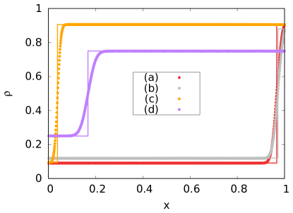
Figure 15: Plots illustrating the density $\rho$ as a function of position $x$ in the DW phase under the strong coupling limit. MFT predictions (colored solid lines) are confirmed with great accuracy by MCS results (colored discrete points), both sharing the same color for a particular set of parameter values. Values of these parameters are as follows: (a) $\alpha=1$, $\beta=0.1$, $\mu=0.3$, $k_{1}=k_{2}=0.95$; (b) $\alpha=1.5$, $\beta=0.13$, $\mu=0.3$, $k_{1}=k_{2}=0.95$; (c) $\alpha=1.5$, $\beta=0.1$, $\mu=1$, $k_{1}=k_{2}=0.95$; and (d) $\alpha=1.5$, $\beta=0.3$, $\mu=1$, $k_{1}=k_{2}=0.95$.

In Fig. 15, DW phase density profiles in the weak coupling limit are obtained. Both the MFT and MCS results demonstrate remarkable consistency and conformity. Additionally, how the DW position ($x_{w}$) and height ($\Delta$) varies with $\mu$ and $k_{1},k_{2}$ is illustrated in Fig. 16 and Fig. 17.

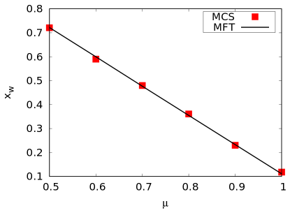
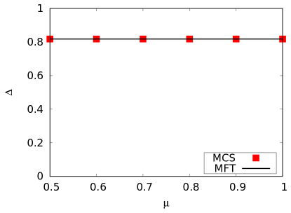
Figure 16: (Left) Plot of the domain wall position $x_{w}$ versus $\mu$ in the strong coupling limit of the model. The entry and exit rates are $\alpha=1$ and $\beta=0.1$, and the exchange rates are $k_{1}=k_{2}=0.95$. The location of the domain walls shows a linear decrement with increasing values of $\mu$. The results obtained from both MFT and MCS show similar trends and demonstrate good quantitative agreement. (Right) Plot of the domain wall height $\Delta$ versus $\mu$ in the strong coupling limit of the model with control parameters $\alpha=1$, $\beta=0.1$, and $k_{1}=k_{2}=0.95$. The height of the domain wall remains constant with varying $\mu$. The MFT and MCS results are in reasonable agreement.

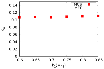
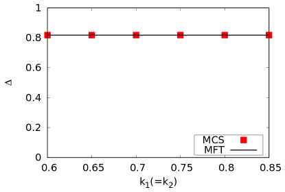
Figure 17: (Left) The left plot illustrates the relationship between the position of a domain wall ($x_{w}$) and the exchange rates ($k_{1}=k_{2}$) in the strong coupling regime of the model. The parameters used are an entry rate ($\alpha$) of 1, an exit rate ($\beta$) of 0.1, and a filling factor ($\mu$) of 1. Specific to these parameter values, the location of the domain wall remains constant as the exchange rates vary within the observed range. The results obtained from MFT and MCS show good agreement. (Right) The right plot displays the variation of the domain wall height ($\Delta$) with respect to the exchange rates ($k_{1}=k_{2}$) in the strong coupling regime of the model. The control parameters utilised are an entry rate ($\alpha$) of 1, an exit rate ($\beta$) of 0.1, and a filling factor ($\mu$) of 1. The height of the domain wall remains constant as long as the exchange rates are equal. The results from MFT and MCS exhibit a good agreement.

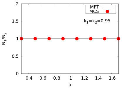
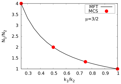
Figure 18: (Left) The plot shows how the reservoir population ratio $N_{1}/N_{2}$ varies with the filling factor $\mu$ in the strong coupling limit of the model. The exchange rates $k_{1}$ and $k_{2}$ are fixed at 0.95. The entry and exit rates are chosen to ensure that the TASEP lane remains in the LD phase. The values of $\alpha=0.1$ and $\beta=1$ are used. There is good agreement between the mean-field theory (MFT) and Monte Carlo simulations (MCS) results. (Right) The plot illustrates the dependence of the reservoir population ratio $N_{1}/N_{2}$ on the exchange rate ratio $k_{1}/k_{2}$ for a fixed filling factor $\mu=3/2$ in the strong coupling limit. The entry and exit rates are again chosen to keep the system in the LD phase, i.e, $\alpha=0.1$ and $\beta=1$. Both MFT and MCS results show a consistent behavior.

To get the LD-DW and HD-DW phase boundaries, one sets $x_{w}=1$ and $x_{w}=0$ respectively in eq. (104). Thus, with $x_{w}=1$, the LD-DW boundary is determined to be

$$\bigg{(}1+\alpha-\frac{\alpha}{\beta}\bigg{)}\bigg{(}\frac{k_{2}}{k_{1}+\frac{\alpha}{\beta}k_{2}}\bigg{)}=\mu-1.$$ (110)

Likewise with $x_{w}=0$, the HD-DW boundary is obtained as

$$\bigg{(}1-\alpha-\frac{\alpha}{\beta}\bigg{)}\bigg{(}\frac{k_{2}}{k_{1}+\frac{\alpha}{\beta}k_{2}}\bigg{)}=\mu-2.$$ (111)

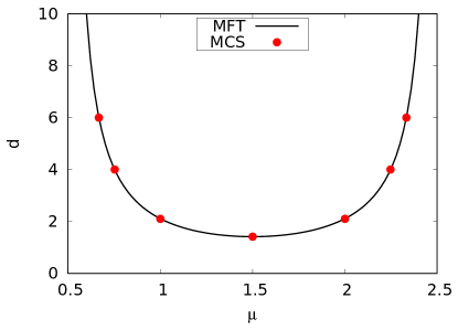
Figure 19: Plot of the distance $d$ between the origin and the multicritical point versus filling factor $\mu$ in the strong coupling limit of the model. Particle exchage rates between reservoirs are taken to be same, i.e., $k_{1}=k_{2}=0.95$. Black solid line and the discrete colored points represent the MFT and MCS results respectively, which are in excellent agreement. As $\mu\rightarrow 1/2$ from above or $\mu\rightarrow 5/2$ from below, $d$ diverges.

Analogous to the weak coupling limit, multiple phases can share a common point in the strong coupling limit too. This multicritical point is given by the coordinates

$$(\alpha_{\text{c}},\beta_{\text{c}})=\left(\frac{k_{1}+k_{2}}{(2\mu-1)k_{2}},\frac{k_{1}+k_{2}}{(3-2\mu)k_{1}+2k_{2}}\right),$$ (112)

and exists over the range $1/2<\mu<(3/2+k_{2}/k_{1})$. The distance between the origin $(0,0)$ and the multicritical point is

$$d=\sqrt{\left(\frac{k_{1}+k_{2}}{(2\mu-1)k_{2}}\right)^{2}+\left(\frac{k_{1}+k_{2}}{(3-2\mu)k_{1}+2k_{2}}\right)^{2}}.$$ (113)

The distance $d$ diverges as $\mu$ approaches $1/2$ from above and $(3/2+k_{2}/k_{1})$ from below. The plot of $d$ versus $\mu$ is presented in Fig. 19 with symmetric choice of exchange rates ($k_{1}=k_{2}=0.95$), where MFT and MCS results match well.

B.2 Nature of the phase transitions

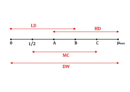
Figure 20: A schematic representation illustrating the ranges of $\mu$ where various phases emerge in the strong coupling limit of the model.

With a structure very similar to what is observed in the weak coupling limit, the model admits two or four phases simultaneously under the strong coupling condition, depending strongly on the value of $\mu$. This is depicted in Fig. 13 and Fig. 14, where particle-hole symmetry is observed only in Fig. 13 where symmetric choices of exchange rates, $k_{1}=k_{2}(=0.95)$, are considered. When transitioning between different phases, the density changes continuosly across the phase boundaries, thus implying second-order phase transitions. Similar transitions were observed in the weak coupling limit. Within a particular range of $\mu$ where all 4 phases exist together in the $\alpha-\beta$ plane, they share a common single point – the multicritical point. In the subsequent discussion, we provide an in-depth analysis of the phases that manifest within a specific range of $\mu$.

See the schematic diagram presented in Fig. 20. Being the thresholds of $\mu$ for the existence of different phases, the points indicated in that figure are as follows:

• A: $\bigg{(}\frac{3}{2}+\frac{k_{2}}{k_{1}}-\frac{k_{2}}{2\beta k_{1}}-\frac{1}{2\beta}\bigg{)}$

• B: $\bigg{(}\frac{1}{2}+\frac{k_{1}}{2\alpha k_{2}}+\frac{1}{2\alpha}\bigg{)}$

• C: $\bigg{(}\frac{3}{2}+\frac{k_{2}}{k_{1}}\bigg{)}$

• $\mu_{\text{max}}=\bigg{(}2+\frac{k_{2}}{k_{1}}\bigg{)}$

The maximum value of $\mu$ is subject to the conditions (92) and (97). We rewrite these conditions together:

$$\mu_{\text{max}}>\bigg{(}\frac{1}{2}+\frac{k_{1}}{2\alpha k_{2}}+\frac{1}{2\alpha}\bigg{)},$$ (114)

$$\mu_{\text{max}}>\bigg{(}\frac{1}{2}+\frac{k_{2}}{2\beta k_{1}}+\frac{1}{2\beta}\bigg{)}.$$ (115)

Clearly, B $\geq$ 1/2 and A $\leq$ C for any (positive) values of $\alpha$, $\beta$, $k_{1}$, and $k_{2}$. The positions of points A and B on the $\mu$-axis depend on the values of $\alpha$, $\beta$, $k_{1}$, and $k_{2}$. Specifically, keeping $k_{1}$ and $k_{2}$ fixed and adjusting the values of $\alpha$ and $\beta$, we can slide points A and B along the $\mu$-axis.

Setting B $\geq$ A, the following condition emerges:

$$\mu_{\text{max}}\leq\bigg{[}1+\frac{1}{2\alpha}\bigg{(}1+\frac{k_{1}}{k_{2}}\bigg{)}+\frac{1}{2\beta}\bigg{(}1+\frac{k_{2}}{k_{1}}\bigg{)}\bigg{]},$$ (116)

which is consistent with the conditions (114) and (115) for $\mu_{\text{max}}$, assuming that the control parameters $\alpha$, $\beta$, $k_{1}$, and $k_{2}$ are all positive values. The other possibility B $<$ A, which results into the condition

$$\mu_{\text{max}}>\bigg{[}1+\frac{1}{2\alpha}\bigg{(}1+\frac{k_{1}}{k_{2}}\bigg{)}+\frac{1}{2\beta}\bigg{(}1+\frac{k_{2}}{k_{1}}\bigg{)}\bigg{]},$$ (117)

is discarded as it is not necessarily true along with the conditions (114) and (115). This implies that the position of point B can be either to the right of point A or coincide with it, but it cannot be to the left of point A.

By analyzing the expressions for points B and C, the following condition for $\alpha$ is obtained when B is positioned to the left of C,

$$\alpha>\frac{\bigg{(}1+\frac{k_{1}}{k_{2}}\bigg{)}}{2\bigg{(}1+\frac{k_{2}}{k_{1}}\bigg{)}}.$$ (118)

For HD-MC phase boundary, given in (101), to be observed in the phase space, the condition $\mu<$ C must be satisfied, failing to meet which leads to negative values of $\beta$ which is unphysical. Substituing the value of $\alpha$ we got at the LD-MC phase boundary (100) in (118) also yields the condition $\mu<$ C. In contrast, when the point B is located to the right side of point C, $\alpha$ takes on the following expression:

$$\alpha<\frac{\bigg{(}1+\frac{k_{1}}{k_{2}}\bigg{)}}{2\bigg{(}1+\frac{k_{2}}{k_{1}}\bigg{)}}.$$ (119)

The condition (119), when put to the LD-MC phase boundary (100), corresponds to the condition $\mu>$ C, for which $\beta<0$. Thus B is limited to move between 1/2 and C. Similarly, point A is constrained to move between 1/2 and C.

To summarise, if the exchange rates $k_{1}$ and $k_{2}$ are held constant while $\alpha$, $\beta$ can be varied, all points except A and B remain fixed along the $\mu$-axis. However, points A and B can be adjusted between the values of 1/2 and C by varying the parameters $\alpha$ and $\beta$. It should be noted that point B cannot be located to the left of point A.

Table 2 provides a summary of the range of $\mu$ in which various phases emerge, outlining essential details on the number and nature of phase boundaries, as well as information about the multicritical points.

Row no.	Range of $\mu$	Phases	Domain walls	Phase boundaries	Multicritical points (MCPs)
1	$0<\mu<\frac{1}{2}$	LD and DW	One LDW	One second-order	None
2	$\frac{1}{2}<\mu<\bigg{(}\frac{3}{2}+\frac{k_{2}}{k_{1}}-\frac{k_{2}}{2\beta k_{1}}-\frac{1}{2\beta}\bigg{)}$	LD, HD, MC, and DW	One LDW	Four second-order	One four-phase MCP
3	$\bigg{(}\frac{3}{2}+\frac{k_{2}}{k_{1}}-\frac{k_{2}}{2\beta k_{1}}-\frac{1}{2\beta}\bigg{)}<\mu<\bigg{(}\frac{1}{2}+\frac{k_{1}}{2\alpha k_{2}}+\frac{1}{2\alpha}\bigg{)}$	LD, HD, MC, and DW	One LDW	Four second-order	One four-phase MCP
4	$\bigg{(}\frac{1}{2}+\frac{k_{1}}{2\alpha k_{2}}+\frac{1}{2\alpha}\bigg{)}<\mu<\bigg{(}\frac{3}{2}+\frac{k_{2}}{k_{1}}\bigg{)}$	LD, HD, MC, and DW	One LDW	Four second-order	One four-phase MCP
5	$\bigg{(}\frac{3}{2}+\frac{k_{2}}{k_{1}}\bigg{)}<\mu<\bigg{(}2+\frac{k_{2}}{k_{1}}\bigg{)}$	HD and DW	One LDW	One second-order	None

Table 2: Table summarizing the occurence of certain phases and phase boundaries within a range of filling factor $\mu$ according to MFT in the strong coupling limit case. Particle-hole symmetry can be seen when a symmetric choice of exchange rates is considered, i.e., $k_{1}=k_{2}$.

Appendix C Steady state density profiles in the LD, HD, and MC phases for both weak and strong coupling limit

In this section, we present the steady state density profiles in the low-density (LD), high-density (HD), and maximal current (MC) phases of the model for both the weak and strong coupling limit cases; see Fig. 21.

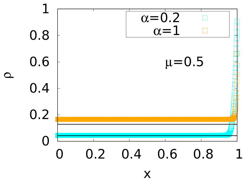
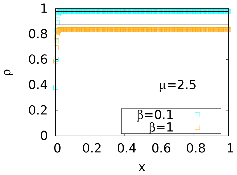
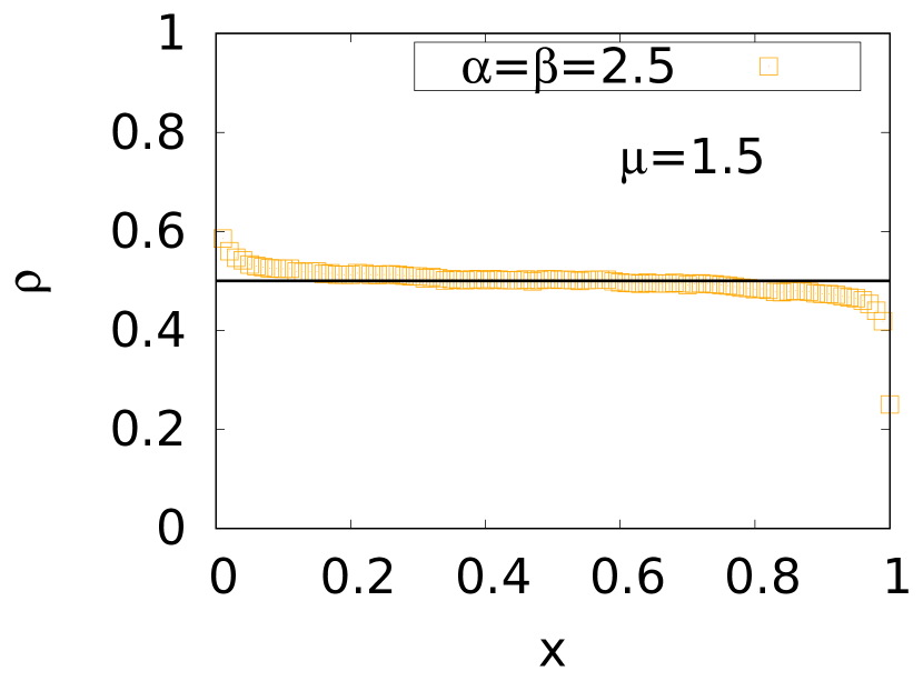
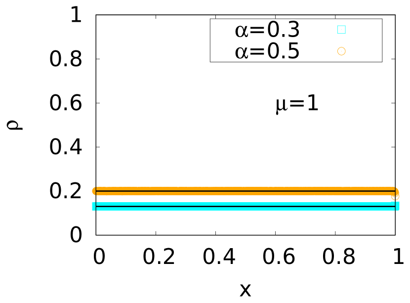
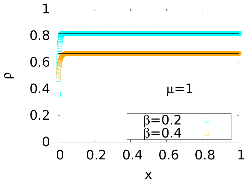
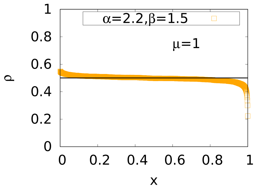
Figure 21: These six plots illustrate the steady state density profiles in the LD, HD, and MC phases under both weak and strong coupling limits. The subfigures in the top row represent the weak coupling limit with exchange rates $k_{10}$ and $k_{20}$ set to 0.95, while those in the bottom row represent the strong coupling limit with exchange rates $k_{1}$ and $k_{2}$ set to 0.7. The values of the control parameters $\alpha$, $\beta$, and $\mu$ are indicated in each subfigure. The solid black lines depict the MFT predictions, and the colored points correspond to the results obtained from MCS. In the weak coupling limit, MFT and MCS results closely match for small values of $\alpha$ and $\beta$. However, as $\alpha$ and $\beta$ increase, disagreement between the densities increases. On the other hand, in the strong coupling limit, MFT and MCS results exhibit a remarkable agreement across the entire parameter range.

Appendix D Simulation algorithm

In this study, the mean-field predicted densities and phase diagrams of the model were validated through Monte Carlo simulations using random updates. The simulation rules are as follows: (i) If the first site ($i=1$) of the TASEP lane ($T$) is empty, a particle from reservoir $R_{1}$ enters $T$ with a rate $\alpha_{\text{eff}}$; (ii) Particles in $T$ can hop with rate 1 to the subsequent site in the bulk of $T$ if that site is empty; (iii) When at the last site ($i=L$) of $T$, a particle exits $T$ with a rate $\beta_{\text{eff}}$ into reservoir $R_{2}$; (iv) Simultaneously with these movements, particles in the reservoirs ($R_{1}$ and $R_{2}$) can jump directly to the other reservoir with definitive rates: $k_{1}N_{1}$ from $R_{1}$ to $R_{2}$ and $k_{2}N_{2}$ from $R_{2}$ to $R_{1}$; and (v) If, for any iteration, $k_{1}N_{1}$ and/or $k_{2}N_{2}$ are greater than 1, the rates are normalised by dividing each rate by the maximum value between $k_{1}N_{1}$ and $k_{2}N_{2}$. In each iteration of the simulation, the reservoirs or a site from the TASEP lane are randomly chosen for updating. After a sufficient number of iterations to reach steady states, the density profiles are calculated, and temporal averages are performed.

References

- (1) S. Katz, J. L. Lebowitz, and H. Spohn, “Phase transitions in stationary nonequilibrium states of model lattice systems,” Phys. Rev. B 28, 1655–1658 (1983).
- (2) S. Katz, J. L. Lebowitz, and H. Spohn, “Nonequilibrium steady states of stochastic lattice gas models of fast ionic conductors,” J. Stat. Phys. , 497–537 (1984).
- (3) B. Schmittmann and R. K.-P. Zia, Phase transitions and critical phenomena, edited by Joel Louis Lebowitz and Cyril Domb (Academic Press, London, 1995).
- (4) Nonequilibrium Statistical Mechanics in One Dimension, (Cambridge University Press, 1997).
- (5) J. Krug, “Boundary-induced phase transitions in driven diffusive systems,” Phys. Rev. Lett. 67, 1882 (1991).
- (6) B. Derrida, S. A. Janowsky, J. L. Lebowitz, and E. R. Speer, “Exact solution of the totally asymmetric simple exclusion process: Shock profiles,” J Stat Phys , 813–842.
- (7) B. Derrida and M. R Evans, “Exact correlation functions in an asymmetric exclusion model with open boundaries,” Journal de Physique I 3, 311–322 (1993).
- (8) B. Derrida, M. R. Evans, V. Hakim, and V. Pasquier, “Exact solution of a 1d asymmetric exclusion model using a matrix formulation,” J. Phys. A: Math. and Gen. 26, 1493–1517 (1993).
- (9) C. T. MacDonald, J. H. Gibbs, and A. C. Pipkin, “Kinetics of biopolymerization on nucleic acid templates,” Biopolymers 6, 1–25 (1968), A 40, R333–R441 (2007).
- (10) D A Adams, B Schmittmann, and R K P Zia, “Far from equilibrium transport with constrained resources,” J. Stat. Mech.: Theory Exp 2008, P06009 (2008).
- (11) M. Ha and M. den Nijs, “Macroscopic car condensation in a parking garage,” Phys. Rev. E 66, 036118 (2002).
- (12) C. A. Brackley, M. C. Romano, C. Grebogi, and M. Thiel, “Limited resources in a driven diffusion process,” Phys. Rev. Lett. 105, 078102 (2010).
- (13) C. A. Brackley, M. C. Romano, and M. Thiel, “Slow sites in an exclusion process with limited resources,” Phys. Rev. E 82, 051920 (2010).
- (14) C. A Brackley, M. C. Romano, and M. Thiel, “The dynamics of supply and demand in mrna translation,” PLoS computational biology 7, e1002203 (2011).
- (15) L. Ciandrini, I. Neri, J. C. Walter, O. Dauloudet, and A. Parmeggiani, “Motor protein traffic regulation by supply–demand balance of resources,” Phys. biol. 11,
- (16) M. C. Good, M. D. Vahey, A. Skandarajah, D. A. Fletcher, and R. Heald, “Cytoplasmic volume modulates spindle size during embryogenesis,” Science 342, 856–860 (2013).
- (17) J. Hazel, K. Krutkramelis, P. Mooney, M. Tomschik, K. Gerow, J. Oakey, and JC Gatlin, “Changes in cytoplasmic volume are sufficient to drive spindle scaling,” Science 342, 853–856 (2013).
- (18) L. Jonathan Cook, R. K. P. Zia, “Feedback and fluctuations in a totally asymmetric simple exclusion process with finite resources,” J. Stat. Mech.: Theory Exp 2009, P02012 (2009).
- (19) L. Jonathan Cook, R. K. P. Zia, and B. Schmittmann, “Competition between multiple totally asymmetric simple exclusion processes for a finite pool of resources,” Phys. Rev. E 80, 031142 (2009).
- (20) C. A Brackley, L. Ciandrini, and M C. Romano, “Multiple phase transitions in a system of exclusion processes with limited reservoirs of particles and fuel carriers,” J. Stat. Mech.: Theory Exp 2012, P03002 (2012).
- (21) A. Haldar, P. Roy, and A. Basu, “Asymmetric exclusion processes with fixed resources: Reservoir crowding and steady states,” Phys. Rev. E 104, 034106 (2021).
- (22) A. Robson, K. Burrage, and M. C. Leake, Inferring diffusion in single live cells at the single-molecule level, Philos Trans R Soc (Lond) B Biol Sci. 368(1611), 20120029 (2013) [DOI: doi: 10.1098/rstb.2012.0029]
- (23) H. Hinsch and E. Frey, “Bulk-driven nonequilibrium phase transitions in a mesoscopic ring,” Phys. Rev. Lett. 97, 095701 (2006).
- (24) P. Roy, A. K. Chandra and A. Basu, “Pinned or moving: states of a single shock in a ring,” Phys. Rev. E 102, 012105 (2020).
- (25) Atri Goswami, Mainak Chatterjee, Sudip Mukherjee, “Steady states and phase transitions in heterogeneous asymmetric exclusion processes,” J. Stat. Mech. - Th. Exp. 123209 (2022).
- (26) R A Blythe and M R Evans, “Nonequilibrium steady states of matrix-product form: a solver’s guide,” J. Phys. A 40, R333–R441 (2007).
- (27) T. Franosch A. Melbinger, T. Reichenbach and E. Frey, “Driven transport on parallel lanes with particle exclusion and obstruction,” Phys. Rev. E 83, 031923 (2011).