Equilibration between Translational and Rotational Modes in Molecular Dynamics Simulations of Rigid Water Requires a Smaller Integration Time-Step Than Often Used

Abstract

In simulations of aqueous systems it is common to freeze the bond vibration and angle bending modes in water to allow for a longer time-step $\delta t$ for integrating the equations of motion. Thus $\delta t=2$ fs is often used in simulating rigid models of water. We simulate the SPC/E model of water using $\delta t$ from 0.5 fs to 3.0 fs. We find that for all but $\delta=0.5$ fs, equipartition between translational and rotational modes is violated: the rotational modes are at a lower temperature than the translation modes. The autocorrelation of the velocities corresponding to the respective modes shows that the rotational relaxation occurs at a time-scale comparable to vibrational periods, invalidating the original assumption for freezing vibrations. $\delta t$ also influences thermodynamic properties: the mean system potential energies are not converged until $\delta t=0.5$ fs, and the excess entropy of hydration of a soft, repulsive cavity is also sensitive to $\delta t$.

Water is the matrix of life, and a molecular level understanding of biological processes is predicated on understanding how the bio-molecules are influenced by the liquid water matrix ¹. Thus, developing better ways to describe the structure and dynamics of water has come to occupy a central position in computational (bio)molecular sciences.

Rahman and Stillinger, the early pioneers in simulating water using molecular dynamics, described water as a rigid object and numerically solved for the coupled translational and rotational motion of each water molecule in the liquid^{2, 3}. In their numerical scheme, the translational motion of the center of mass was formulated in terms of Cartesian coordinates and the rotational motion was formulated in terms of Euler angles. The Hamiltonian of the system was based on a sum of Lennard-Jones and electrostatic contributions. Using the mass $m$ of the water molecule, the Lennard-Jones well-depth $\varepsilon$, and collision diameter $\sigma$, they identified the natural unit of time in the equations of motion to be $\tau=\sigma\cdot\sqrt{m/\varepsilon}\approx 2$ ps ². From numerical experiments on a two-molecule system, they found that to integrate the coupled set of equations, they had to use a time-step $\delta t=2\times 10^{-4}\tau\approx 0.4$ fs. They noted that the smallness of this time-step, relative to modeling liquid Ar, for example, stemmed from the “rapid angular velocity of the water molecules” ². We shall return to this point below.

A few years after Rahman and Stillinger’s work, Ryckaert, Ciccotti, and Berendsen developed the SHAKE algorithm⁴ to incorporate holonomic constraints in simulating various types of molecules, including water. For simulating a rigid model of water, one choice of constraints could be OH bond lengths and a pseudo-bond between the two protons. These holonomic constraints lead to additional forces in the dynamical equations, but the significant computational advantage one gains is in formulating all the equations in Cartesian coordinates. Later, Andersen noted that in simulating a rigid object, the relative velocity of atoms mutually tied by a rigid bond should be zero in the direction of the bond. Andersen developed the RATTLE algorithm to include this velocity constraint ⁵. More than a decade after Andersen’s work, Miyamoto and Kollman ⁶ presented an algorithm specifically for describing water as a rigid molecule. This so-called SETTLE algorithm obviated the iterations implicit in the SHAKE or RATTLE methods. Like SHAKE, the RATTLE and SETTLE methods require only Cartesian coordinates.

One of the motivations in developing the SHAKE and subsequent algorithms noted above was to freeze the high-frequency vibrations between bonded pairs of atoms, since the “fast internal vibrations are usually decoupled from rotational and translational motions” ⁴. Since typical vibrational frequencies are about $10^{14}$ Hz (or a time period of 10 fs), the intuitive idea was that freezing the high-frequency vibrations ought to allow for a longer $\delta t$ for integrating the equations of motion in molecular simulations. Thus, in the case of simulating rigid water using molecular dynamics, it is very common to use $\delta t=2$ fs; for example, see Refs. 7, 8, 9. We have used this as well in many of our papers, for example, Ref. 10. A well-cited paper on protein folding has used $\delta t=2.5$ fs ¹¹. Some recent efforts use $\delta t=4$ fs, albeit by using a larger proton mass (personal communications, CECAM 2023 meeting on Biomolecular Simulation and Machine Learning in the Exa-Scale era).

What is the problem then? In simulation studies on liquid water under super-cooled conditions using the Langevin thermostat (Valiya Parambathu and Asthagiri, unpublished), one of us (DNA) noticed that the average temperature from the simulation log was systematically lower than the target by about 1 K. We found the same trend in simulations of hydration of a small amphiphile, tert-butanol. This motivated us to examine more thoroughly the distribution of kinetic energy between translational and rotational degrees in simulations of the rigid SPC/E¹² water model. This examination leads to the finding that for $\delta t\geq 1$ fs, equipartition between translation and rotation is violated, with the problem made worse as $\delta t$ increases. We examine the reason for this and find that $\delta t\geq 1$ limits how well one can capture the fast rotational relaxation. The $\delta t=0.5$ fs that allows thermalization between rotation and translation is also surprisingly close to what Rahman and Stillinger² used. The violation of equipartition also reveals itself in the $\delta t$ dependence of the mean potential energy of the system and in the excess entropy of hydration of a soft, repulsive cavity.

We study the SPC/E¹² water model using the NAMD^{13, 14} and LAMMPS^{15, 16} codes. For NVT simulations, we obtain results using the stochastic velocity rescaling ¹⁷ and Langevin thermostats, respectively, both of which should correctly sample the canonical distribution. We study two system sizes, $N=2006$ water molecules, which informs the results in the main text, and a limited set of simulations with $N=16384$ water molecules noted in the Supplementary Information (SI). The SI provides a complete description of the methods (SI Sec. 2) and additional supporting results (SI Sec. 3).

From $NVT$ simulations we sample 1050 water molecules (SI Sec. 2.2). From the coordinates and velocities of the atoms at a given time point for a sampled water molecule, we calculate the translational kinetic energy of the center of mass and the kinetic energy for rotation about the center of mass. For a canonical ensemble, these kinetic energy contributions must follow the Maxwell-Boltzmann distribution: specifically, for a single degree of freedom, the mean kinetic energy is $k_{\rm B}T/2$ and the variance is $(k_{\rm B}T)^{2}/2$. This allows us to calculate $T$ following two different paths (SI Sec. 1). The different paths lead to the same estimate of $T$ within statistical uncertainties, as they should for well-converged simulations.

Figure 1 shows that the temperatures ascribable to the different modes converge only for $\delta t=0.5$ fs.

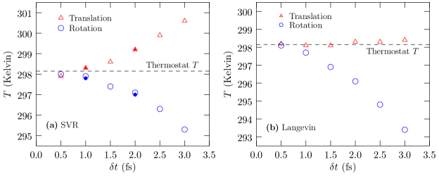
Figure 1: Temperature distribution between the translational and rotational modes in simulations of SPC/E water. The temperatures are based on the mean kinetic energy path. Results using (a) SVR and (b) Langevin thermostats. The open symbols are based on simulations with NAMD ^{13, 14}. The symbol size is about $2\sigma$ standard error of the mean. The filled symbols in (a) are based on simulations using LAMMPS ^{15, 16}.

For the Langevin thermostat with $\delta t=2.0$ fs, the mean of the translational and rotational temperatures is about 297 K, a Kelvin lower than the set-point, consistent with the earlier observations for supercooled water and the hydration of the amphiphile that motivated the present work. Similar deviations persist in constant energy (NVE) simulations as well (SI Sec. 3.4), emphasizing that the data in Figure 1 is not an artifact of the thermostat.

To better understand the results shown in Figure 1, it proves helpful to examine the velocity autocorrelation function. To this end, we take the last configuration of the $\delta t=0.5$ fs run with the SVR thermostat and launch constant energy runs for 20 ps saving velocities and positions every time step. For NVE starting velocities, we use the same seed for the random number generator for the different $\delta t$ cases. Figure 2 shows the velocity autocorrelation using the data from the $\delta t=0.5$ fs simulations, our reference. In passing, we note that the integral of the velocity autocorrelation gives the diffusion coefficient through the Green-Kubo relations. As a check, for $\delta t=0.5$ fs we find the translational diffusion coefficient using both the Green-Kubo approach and the Einstein relation (SI Sec. 3.6) for the mean squared displacement. These estimates agree within statistical uncertainties.

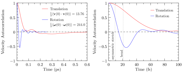
Figure 2: Autocorrelation of the center of mass and angular velocities normalized by the value at time $t=0$. Left panel: data shown out to 0.6 ps. Right panel: data shown to 100 fs. The time periods associated with the asymmetric stretch and bending modes of a water molecule in the gas phase ¹⁸ are also shown for comparison.

What is striking about Fig. 2 (left panel) is that the rotational motion relaxes considerably faster than the translational motion — observe that the $t=0$ value is much higher and the decay much faster for the autocorrelation of the angular velocity. This is consistent with what Rahman and Stillinger² noted. Physically, the rotational relaxation is considerably faster than the translation relaxation because, in contrast to the translational movement of the entire mass, the small mass of the proton relative to that of the oxygen means that the moment of inertia is small and rotations are sensitive to small torques.

As Fig. 2 (right panel) shows, the rotational relaxation occurs over time scales that are similar to the time period of the bond vibration and angle bending modes of a water molecule in the gas phase. For a water molecule in the liquid, because of hydrogen bonding interactions these modes will be “softened” and shift to the right and spread out ¹⁸. So, even using the worst case estimate of a water molecule in the gas phase, we find that the original motivation for freezing vibrations is not well-founded for describing liquid water.

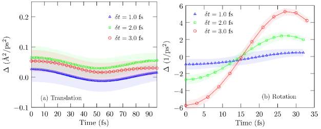
Figure 3: $\Delta$ is the difference at a given time point between the autocorrelation for the given $\delta t$ minus the corresponding reference value using $\delta t=0.5$ fs. For no discretization error, $\Delta=0$. (a): Translational, and (b): Rotational motion. The shaded area indicates $1\sigma$ standard error of the mean.

Figure 3 shows the difference between the velocity autocorrelation obtained using a given $\delta t$ and the reference value based on $\delta t=0.5$ fs (Fig. 2). We focus on the initial times as this is the more important and more sensitive part of the overall relaxation. It is immediately clear that discretization of the equations of motion limits the fidelity with which we can assess the corresponding relaxation. For the translational motion (Fig. 3, left panel), the differences at initial times are all positive. However, the net impact on the diffusion coefficient as assessed by the Einstein relation is small (SI Sec. 3.6); this suggests that integrating the overall autocorrelation can smooth out errors and mask the role of $\delta t$. Similarly, for the rotational motion (Fig. 3, right panel), we find that the autocorrelation up to about 15 fs is lower than the reference value. Notice the stark contrast in the magnitude of deviations relative to the reference autocorrelation. Since the rotational relaxation occurs on a considerably shorter time scale (and involves larger magnitudes), it is also more sensitive to discretization: large $\delta t$ leads to large errors in describing rotational relaxation than it does for translation relaxation.

We can use the fluctuation-dissipation relation $\mathcal{D}=k_{\rm B}T/\xi$, where $\mathcal{D}$ is the diffusion coefficient, $\xi$ is the friction, and $k_{\rm B}T$, to interpret the results above. Treating $\xi/k_{\rm B}T$ as an “effective” friction, and solely focusing on the initial time behavior of the autocorrelation, we can infer that the “effective” friction appears to be higher for rotational motion and lower for translational motion relative to the $\delta t=0.5$ fs reference. Friction arises due to inter-molecular interactions. Since the same potential model is used for all $\delta t$ values, a high “effective” friction is a consequence of lower temperature and vice versa, in agreement with results in Fig. 1.

We hypothesized that the discrepancy in thermalization between rotational and translational motions ought to influence properties besides initial relaxation, including thermodynamic properties such as the excess entropy. To test this hypothesis, we first calculated the mean binding energy, $\langle\varepsilon\rangle$, of a water molecule with the rest of the system (SI Sec. 2.1.4) — the mean potential energy of the $N$ water molecule system is $N\langle\varepsilon\rangle/2$. Fig, 1 (left panel) shows that the mean binding energy is indeed sensitive to $\delta t$, with the values obtained using different thermostats converging only for $\delta t=0.5$ fs. Specifically, for $\delta t=3$ fs, the mean potential energy per water molecule differs by 0.3% between the two thermostats; for $\delta t=0.5$ fs the deviation drops to 0.03%.

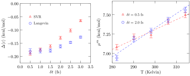
Figure 4: Left panel: Mean binding (interaction) energy of a water molecule with the rest of the system. $\Delta\langle\varepsilon\rangle=\langle\varepsilon\rangle-22$. The standard error of the mean value is at the 2$\sigma$ level. Note that a deviation of 0.1 kcal/mol per particle amounts to $\approx 200$ kcal/mol for the entire system. Right panel: $\delta t$ dependence of the hydration free energy of a soft, repulsive cavity. The standard error of the mean is shown at 1$\sigma$ level.

Fig. 4 (right panel) shows the hydration free energy of a soft, repulsive cavity of size 4 Å (SI Sec. 2.3) as a function of temperature. The excess entropy of hydration at 298.15 K obtained from a linear fit to the $\mu^{{\rm ex}}$ data is $-12.8\pm 0.1$ cal/mol-K for $\delta t=0.5$ fs and $-18.6\pm 0.1$ cal/mol-K for $\delta t=2.0$ fs, a nearly 50% difference. The free energies themselves are about the same at 298.15 K, suggesting compensation between enthalpic and entropic effects.

The identification of fast rotational relaxation of water by us is certainly not new. For example, an early pioneering study by Lawrence and Skinner¹⁹ (see their Figure 4) conveys this point, as does Figure 2 in this work. It is encouraging, and also humbling, that Rahman and Stillinger² chose a small $\delta t$ to better describe the fast angular relaxation, especially at a time when simulations were a lot more demanding than they are now. However, the key finding of our work is that not capturing the fast rotational relaxation of water can break equipartition itself. Further, our work shows that the relaxation of the bond vibrations of water occur at a time scale similar to the rotational relaxation in the rigid model of water studied here, and thus the original motivation for using SHAKE (or SETTLE) for water can be questioned.

Earlier researchers^{20, 21, 22} have shown that in discrete Hamiltonian dynamics the evolution of the system follows a so-called shadow Hamiltonian, which is a function of $\delta t$ (SI Sec. 3.3). This confounds the relationship between momentum (which is what one calculates using the “velocity”-Verlet equations) and velocity in classical mechanics²¹. Thus it has been argued that the Velocity Verlet velocities are not the most appropriate quantities for estimating the temperature ^{21, 22}. Despite this, the on-step “Velocity” Verlet velocities are the quantities used in most codes for calculating the instantaneous temperature. Importantly, our identification of the breakdown of equipartition (Fig. 1), and the thermodynamic consequences of using a large step size (Fig. 4) does emphasize the need to use a smaller $\delta t$ than has been used in numerous studies of liquid water. Our study here also suggests caution in using larger step sizes in aqueous bio-molecular simulations by changing the proton mass (SI Sec. 3.5).

We leave it to future studies to re-examine earlier significant results in aqueous phase chemistry and biology that are founded on molecular simulations using a large time step. The findings here are also expected to be relevant to the modeling of rate processes that are sensitive to solvent friction, to efforts in coarse-graining simulations, and in the development and benchmarking of forcefields.

1 Supporting Information

Supporting Information includes (1) a brief discussion of how temperature is related to the kinetic energy and the fluctuation of kinetic energy, (2) methodology — simulation systems, codes, time steps, calculation of translational and rotational kinetic energy, and calculation of the hydration free energy of a soft, repulsive cavity, and (3) Supplemental results — tabulated data for results in Figure 1, data for relative velocity along constrained bonds, sampling of the shadow Hamiltonian, translational and rotational energy in NVE simulations, influence of the proton mass for $\delta t=4$ fs, and mean-squared displacement for translational diffusion coefficient.

2 Acknowledgements

We thank Arjun Valiya Parambathu (U. Delaware), Thiago Pinheiro dos Santos (Rice University), Lawrence Pratt (Tulane University), Van Ngo (ORNL), and David Rogers (ORNL) for helpful discussions, and Nick Hagerty (OLCF) for help with LAMMPS on Summit and Frontier supercomputers. This research used resources of the Oak Ridge Leadership Computing Facility at the Oak Ridge National Laboratory, which is supported by the Office of Science of the U.S. Department of Energy under Contract No. DE-AC05-00OR22725.

References

- Ball 2008 Ball, P. Water as an Active Constituent in Cell Biology. Chem. Rev. 2008, 108, 74–108
- Rahman and Stillinger 1971 Rahman, A.; Stillinger, F. H. Molecular Dynamics Study of Liquid Water. J. Chem. Phys. 1971, 55, 3336–3359
- Stillinger and Rahman 1974 Stillinger, F. H.; Rahman, A. Improved Simulation of Liquid Water by Molecular Dynamics. J. Chem. Phys. 1974, 60, 1545–1557
- Ryckaert et al. 1977 Ryckaert, J. P.; Ciccotti, G.; Berendsen, H. J. C. Numerical Integration of the Cartesian Equations of Motion of a System with Constraints: Molecular Dynamics of n-alkanes. J. Comput. Phys. 1977, 23, 327–341
- Andersen 1983 Andersen, H. C. Rattle: A Velocity Version of the Shake Algorithm for Molecular Dynamics Calculations. J. Comput. Phys. 1983, 52, 24–34
- Miyamoto and Kollman 1992 Miyamoto, S.; Kollman, P. A. Settle: An Analytical Version of the SHAKE and RATTLE Algorithm for Rigid Water Models. J. Comput. Chem. 1992, 13, 952–962
- Hummer et al. 2001 Hummer, G.; Rasaiah, J. C.; Noworyta, J. P. Water Conduction Through the Hydrophobic Channel of a Carbon Nanotube. Nature 2001, 414, 188–190
- Paschek 2004 Paschek, D. Temperature Dependence of the Hydrophobic Hydration and Interaction of Simple Solutes: An Examination of Five Popular Water Models. J. Chem. Phys. 2004, 120, 6674–6690
- Godawat et al. 2009 Godawat, R.; Jamadagni, S. N.; Garde, S. Characterizing Hydrophobicity of Interfaces by using Cavity Formation, Solute Binding, and Water Correlations. Proc. Natl. Acad. Sci. USA 2009, 106, 15119–15124
- Tomar et al. 2020 Tomar, D. S.; Paulaitis, M. E.; Pratt, L. R.; Asthagiri, D. N. Hydrophilic Interactions Dominate the Inverse Temperature Dependence of Polypeptide Hydration Free Energies Attributed to Hydrophobicity. J. Phys. Chem. Lett. 2020, 11, 9965–9970
- Lindorff-Larsen et al. 2011 Lindorff-Larsen, K.; Piana, S.; Dror, R. O.; Shaw, D. E. How Fast-Folding Proteins Fold. Science 2011, 334, 517–20
- Berendsen et al. 1987 Berendsen, H. J. C.; Grigera, J. R.; Straatsma, T. P. The Missing Term in Effective Pair Potentials. J. Phys. Chem. 1987, 91, 6269–6271
- Kale et al. 1999 Kale, L.; Skeel, R.; Bhandarkar, M.; Brunner, R.; Gursoy, A.; Krawetz, N.; Phillips, J.; Shinozaki, A.; Varadarajan, K.; Schulten, K. NAMD2: Greater Scalability for Parallel Molecular Dynamics. J. Comput. Phys. 1999, 151, 283
- Phillips et al. 2020 Phillips, J. C.; Hardy, D. J.; Maia, J. D. C.; Stone, J. E.; Ribeiro, J. V.; Bernardi, R. C.; Buch, R.; Fiorin, G.; Hénin, J.; Jiang, W. et al. Scalable Molecular Dynamics on CPU and GPU Architectures with NAMD. J. Chem. Phys. 2020, 153, 044130
- Plimpton 1995 Plimpton, S. Fast Parallel Algorithms for Short-Range Molecular Dynamics. J. Comput. Phys. 1995, 117, 1–19
- Thompson et al. 2022 Thompson, A. P.; Aktulga, H. M.; Berger, R.; Bolintineanu, D. S.; Brown, W. M.; Crozier, P. S.; in ’t Veld, P. J.; Kohlmeyer, A.; Moore, S. G.; Nguyen, T. D. et al. LAMMPS - A Flexible Simulation Tool for Particle-Based Materials Modeling at the Atomic, Meso, and Continuum Scales. Comp. Phys. Comm. 2022, 271, 108171
- Bussi et al. 2007 Bussi, G.; Donadio, D.; Parrinello, M. Canonical Sampling Through Velocity Rescaling. J. Chem. Phys. 2007, 126, 014101
- Kananenka and Skinner 2018 Kananenka, A. A.; Skinner, J. L. Fermi Resonance in OH-stretch Vibrational Spectroscopy of Liquid Water and the Water Hexamer. J. Chem. Phys. 2018, 244107
- Lawrence and Skinner 2002 Lawrence, C. P.; Skinner, J. L. Vibrational Spectroscopy of HOD in liquid D2O. I. Vibrational Energy Relaxation. J. Chem. Phys. 2002, 117, 5827–5838
- Toxvaerd 1994 Toxvaerd, S. Hamiltonian for Discrete Dynamics. Phys. Rev. E 1994, 50, 2271–2274
- Gans and Shalloway 2000 Gans, J.; Shalloway, D. Shadow Mass and the Relationship Between Velocity and Momentum in Symplectic Numerical Integration. Phys. Rev. E 2000, 61, 4587–4592
- Eastwood et al. 2010 Eastwood, M. P.; Stafford, K. A.; Lippert, R. A.; Jensen, M. Ø.; Maragakis, P.; Predescu, C.; Dror, R. O.; Shaw, D. E. Equipartition and the Calculation of Temperature in Biomolecular Simulations. J. Chem. Theory Comput. 2010, 6, 2045–2058