Shedding light on the MRI driven dynamo in a stratified shearing box

Abstract

We study the magneto-rotational instability (MRI) dynamo in a geometrically thin disc ($H/R\ll 1$) using stratified zero net flux (ZNF) shearing box simulations. We find that mean fields and EMFs oscillate with a primary frequency $f_{\rm dyn}=0.017$ ($\approx 9$ orbital period), but also have higher harmonics at $3f_{\rm dyn}$. Correspondingly, the current helicity, has two frequencies $2f_{\rm dyn}$ and $4f_{\rm dyn}$ respectively, which appear to be the beat frequencies of mean fields and EMFs as expected from the magnetic helicity density evolution equation. Further, we adopt a novel inversion algorithm called the ‘Iterative Removal Of Sources’ (IROS), to extract the turbulent dynamo coefficients in the mean-field closure using the mean magnetic fields and EMFs obtained from the shearing box simulation. We show that an $\alpha-$effect ($\alpha_{yy}$) is predominantly responsible for the creation of the poloidal field from the toroidal field, while shear generates back a toroidal field from the poloidal field; indicating that an $\alpha-\Omega$-type dynamo is operative in MRI-driven accretion discs. We also find that both strong outflow ($\bar{v}_{z}$) and turbulent pumping ($\gamma_{z}$ ) transport mean fields away from the mid-plane. Instead of turbulent diffusivity, they are the principal sink terms in the mean magnetic energy evolution equation. We find encouraging evidence that a generative helicity flux is responsible for the effective $\alpha$-effect. Finally, we point out potential limitations of horizontal ($x-y$) averaging in defining the ‘mean’ on the extraction of dynamo coefficients and their physical interpretations.

1 Introduction

The problem of angular momentum transport is a key concept in a rotationally supported accretion disc (for a review, see Balbus & Hawley 1998). The current consensus is that a weak magnetic field instability, namely magneto-rotational instability (MRI; Velikhov 1959; Chandrasekhar 1960; Balbus & Hawley 1991, 1992) is responsible for outward angular momentum transport and drives mass accretion in a sufficiently ionized accretion disc. Although linear MRI ensures outward angular momentum transport, it must be studied in the non-linear phase to account for different observable phenomena in accretion discs.

MRI in an accretion disc is either studied in a local set-up (shearing box; Balbus & Hawley 1992; Brandenburg et al. 1995; Hawley et al. 1995; Davis et al. 2010; Shi et al. 2010; Bodo et al. 2014; Bhat et al. 2016) or in a global simulation (Stone et al. 1999; Hawley 2001; Hawley et al. 2013; Beckwith et al. 2011; Parkin & Bicknell 2013; Hogg & Reynolds 2016; Dhang & Sharma 2019; Dhang et al. 2023). While a global approach is more desirable, it is computationally expensive. On the other hand, the shearing box approach offers an alternate path which is computationally less costly and can provide deep insights into the local processes in MRI-driven turbulence.

In the shearing-box approach (Goldreich & Lynden-Bell 1965), we expand fluid equations to the lowest order of $H/R$, where $H$ is the density scale height and $R$ is the local radius. Therefore, this approach is valid only for geometrically thin discs with $H/R\ll 1$. Depending on whether the vertical component of gravity ($g_{z}=-\Omega^{2}z$) (producing a vertically stratified gas density) is considered in the momentum equation or not, shearing box simulations are of two types: stratified ($g_{z}\neq 0$) and unstratified ($g_{z}=0$). Further, depending on whether the computational domain can contain net magnetic fields, shearing box models can be classified into zero net flux (ZNF) and net flux (NF) models. Therefore, four possible combinations of the shearing-box model are: i) unstratified ZNF, ii) unstratified NF, iii) stratified ZNF and iv) stratified NF. This work considers a stratified ZNF shearing box model to explore the MRI dynamo in saturation.

Shearing box simulations provide a wide range of behaviour (e.g., convergence, turbulence characteristics etc.) depending on the shearing box model used (for details, we refer to readers to see Table 1 in Ryan et al. (2017)). However, it is to be noted that we will restrict our discussion to the isothermal (i.e. sound speed is constant) models where there is no explicit dissipation and the numerical algorithms provide the dissipation through truncation error at the grid scale. In the presence of an NF, unstratified shearing box simulations show a convergence (in terms of accretion stresses) and sustained turbulence (Hawley et al. 1995; Guan et al. 2009; Simon et al. 2009). On the other hand, stratified NF simulations present different accretion stresses depending on the net flux strength and sustained turbulence (Guan & Gammie 2011; Bai & Stone 2013). Unstratified ZNF models showed intriguing behaviour. Earlier isothermal Unstratified ZNF studies (Fromang & Papaloizou 2007; Pessah et al. 2007) found decreased accretion stress and turbulence with increased resolution, implying non-convergence. However, later Shi et al. (2016) recovered convergence using a box with a larger vertical extent than the radial extent. On the contrary, earlier stratified ZNF models (Davis et al. 2010) suggested that the models are converged till the resolution $128/H$; however, recent studies (Bodo et al. 2011; Ryan et al. 2017) found the model loses convergent properties at higher resolution.

The convergence problem is closely related to the magnetic energy generation process in the MRI-driven flow. For the ZNF (absence of net flux) models, an MRI-driven dynamo must act to overcome the diffusion and sustain the zero net flux in the accretion flow. Earlier ZNF simulations in unstratified (Shi et al. 2016) and stratified (Davis et al. 2010; Bodo et al. 2014; Ryan et al. 2017) shearing boxes found MRI turbulence can self-generate large-scale magnetic fields attaining quasi-stationarity and sustaining turbulence. Riols et al. (2013) suggested that the non-linear MRI does not behave like a linear instability; rather, it provides a pathway for saturation via a subcritical dynamo process. This leads to the question of what kind of dynamo can be sustained in the MRI-driven accretion flow, small-scale or large-scale? The lack of convergence in ZNF models was attributed to the low numerical Prandtl number (Fromang & Papaloizou 2007; however, see Simon et al. 2009) and hence the inefficiency of small-scale dynamo to operate at small Prandtl number (Schekochihin et al. 2005; Bodo et al. 2011). However, it is unclear what happens when convergence is recovered in unstratified ZNF simulations with tall boxes (Shi et al. 2016).

Studying MRI dynamo is also important for understanding the generation of coherent large-scale magnetic fields determining the level of transport (Johansen et al. 2009; Bai & Stone 2013) and outflows in the accretion disc (von Rekowski et al. 2003; Stepanovs et al. 2014; Mattia & Fendt 2022). MRI, in principle, can generate magnetic fields coherent over several scale-heights (Dhang et al. 2023) and acts locally as a mean field in the absence of any external flux influencing convergence and the disc dynamics.

Generally, stratified models generate a more coherent large-scale field over the unstratified models (for a comparison, see Shi et al. 2016). Cyclic behaviour of azimuthally averaged magnetic fields (mean fields), popularly known as the butterfly diagram, is a typical feature observed in the stratified shearing box simulations (Brandenburg et al. 1995; Gressel 2010; Bodo et al. 2014; Ryan et al. 2017; Gressel & Pessah 2022). However, note that the presence of a strong magnetic net flux (Bai & Stone 2013; Salvesen et al. 2016), convection (Hirose et al. 2014; Coleman et al. 2017) etc. can alter the periodicity in the butterfly diagram. Although the cyclic behaviour of mean fields can be explained by invoking the interplay between shear and helicity (Brandenburg & Donner 1997; Gressel & Pessah 2015), some features, such as upward migration of the mean fields, still demand an explanation.

Several studies attempted to understand the underlying mechanism of MRI dynamo using different approaches. While some of the studies (Lesur & Ogilvie 2008; Bai & Stone 2013; Shi et al. 2016; Begelman & Armitage 2023) invoked toy models to complete the generation cycles of radial and azimuthal fields, others (local: Brandenburg et al. 2008; Gressel 2010; Shi et al. 2016; Gressel & Pessah 2022; Mondal & Bhat 2023, global: Dhang et al. 2020) used mean-field theory to investigate the large-scale field generation in the MRI-driven turbulent accretion flow. Most of the studies characterising the turbulent dynamo coefficients in the regime of mean-field dynamo theory used state of the art ‘Test Field’ (TF) method (Gressel 2010; Gressel & Pessah 2015), while a few used direct methods such as linear regression (Shi et al. 2016), singular value decomposition (SVD; Dhang et al. 2020) to calculate dynamo coefficients in post-process or statistical simulations to carry out combined study of the large-scale dynamo and angular-momentum transport in accretion discs (Mondal & Bhat 2023). In this work, we use a direct method, a variant of the cleaning algorithm ( Högbom CLEAN method; Högbom 1974), called ‘Iterative Removal Of Sources’ (IROS; Hammersley et al. 1992); mainly used in astronomical image construction to analyse MRI-dynamo in the mean-field dynamo paradigm. We modified the IROS method according to our convenience (for details, see section 4, also see Bendre et al. 2023) and used it to determine the dynamo coefficients by post-processing the data obtained from the stratified ZNF shearing box simulation.

The paper is organised as follows. In section 2, we describe details of shearing box simulations, basics of mean field closure used and techniques of the IROS method. Section 3 describes the evolution of MRI to a non-linear saturated state, spatio-temporal variations of mean magnetic fields, EMFs and periodicities present in different observables. The spatial profiles of calculated turbulent dynamo coefficients, the reliability of the calculation method (using both EMF reconstruction and a 1D dynamo model) and contributions of each coefficient to the mean magnetic energy equation are described in section 4. In section 5, we discuss the plausible reasons behind different periodicities present (in mean magnetic fields, EMFs and helicties), comparison of our work with the previous works, the possible importance of a generative helicity flux and limitations of the averaging scheme and mean-field closure used in decoupling contributions from different dynamo coefficients. Finally we summarized our key results in section 6.

2 Method

2.1 Shearing-box simulation

We perform stratified zero net flux (ZNF) shearing box simulations to study the MRI driven dynamo in a geometrically thin disc ($H/R\ll 1$). To do that, we solve ideal MHD equations in a Keplerian shearing box given by

$$\frac{\partial\rho}{\partial t}+\nabla.\left(\rho\mathbf{v}\right)=0,$$ (1)

$$\frac{\partial\rho\mathbf{v}}{\partial t}+\nabla.\left(\rho\mathbf{v}\mathbf{v}-\mathbf{B}\mathbf{B}\right)+\nabla P=\rho\mathbf{g}_{s}-2\Omega\hat{z}\times\rho\mathbf{v},$$ (2)

$$\frac{\partial\mathbf{B}}{\partial t}=\nabla\times\left(\mathbf{v}\times\mathbf{B}\right)$$ (3)

using the PLUTO code (Mignone et al. 2007) with $x,\ y,\ z$ as the radial, azimuthal and vertical directions respectively. Here, $\rho,\ P,\ \mathbf{v}$ and $\mathbf{B}$ denote density, thermal pressure, velocity and magnetic fields, respectively. The terms $\mathbf{g}_{s}=\Omega^{2}\left(2qx\hat{x}-z\hat{z}\right)$ and $2\Omega\hat{z}\times\rho\mathbf{v}$ represent the tidal expansion of the effective gravity and the Coriolis force respectively with $\Omega$ denoting orbital frequency. We use an isothermal equation of state

$$P=\rho c^{2}_{s},$$ (4)

which makes the energy equation redundant. Additionally, we use constrained transport (Gardiner & Stone 2005) to maintain divergence free condition

$$\nabla.\mathbf{B}=0$$ (5)

for magnetic fields. We use the HLLD solver (Miyoshi & Kusano 2005) with second-order slope-limited reconstruction. Second-order Runge–Kutta (RK2) is used for time integration with the CFL number 0.33. Also note that despite our shearing-box model lacking explicit dissipation, we refer to it as the direct numerical simulation (DNS).

We initialize an unmagnetized equilibrium solution with density and velocity given by

$$\rho=\rho_{0}\ {\rm exp}\left(-{\frac{z^{2}}{2H^{2}}}\right),$$ (6)

$$\mathbf{v}=-q\ \Omega\ x\ \hat{y}$$ (7)

where $q=1.5$ and $\rho_{0}$ is the mid-plane ($z=0$) density and

$$H=\frac{c_{s}}{\Omega}$$ (8)

is the thermal scale height. We set $\rho_{0}=c_{s}=\Omega=1$, so that $H=1$. Unless stated otherwise, all the length and time-scales are expressed in units of $H$ and $\Omega^{-1}$ respectively. We initialize a ZNF magnetic field given by

$$\mathbf{B}=\sqrt{\frac{2}{\beta_{0}}}\ \sin\left(\frac{2\pi x}{L_{x}}\right)\ \hat{z}$$ (9)

with $\beta_{0}$ defining the strength of the field and $L_{x},\ L_{y},\ L_{z}$ denoting the size of the shearing-box.

Our computational domain extends from $-L_{x}/2<x<L_{x}/2$, $-L_{y}/2<y<L_{y}/2$ and $-L_{z}/2<z<L_{z}/2$. It has been found in earlier studies that shearing box results depend on the domain size; larger boxes tend to capture dynamo better than their smaller counterparts as well as smaller boxes demonstrate a transition to anomalous behaviour (e.g. see Simon et al. 2012; Shi et al. 2016). To avoid these discrepancies, we choose a shearing box of size $L_{x}\times L_{y}\times L_{z}=3H\times 12H\times 8H$ with a grid resolution $N_{x}\times N_{y}\times N_{z}=96\times 192\times 256$ giving rise to a resolution of $32/H$ in the vertical direction. However, we must admit that there exists an issue with the convergence in stratified ZNF models as discussed in the section 1. We reserve the dependence of MRI dynamo on numerical resolution as a topic of future research investigation.

We use periodic and shearing-periodic (Hawley et al. 1995) boundary conditions in the $y$ and $x-$ boundaries, respectively. Outflow boundary conditions are implemented in the vertical ($z$) boundaries. A gradient-free condition is maintained for scalars and tangential components of vector fields at the boundaries. At the same time, $v_{z}\geq 0$ for $z>0$ and $v_{z}\leq 0$ for $z<0$ is set to restrict mass inflow into the domain at vertical boundaries.

2.2 Mean field closure

Before describing the details of mean field dynamo theory and the closure used, we define what is meant by ‘mean’ and ‘fluctuation’ in our work. We define mean magnetic fields ($\mathbf{B}$) as the $x-y$-averaged values as follows

$$\bar{\mathbf{B}}(z,t)=\frac{1}{L_{x}L_{y}}\int_{-L_{x}/2}^{L_{x}/2}\int_{-L_{y}/2}^{L_{y}/2}\mathbf{B}(x,y,z,t)\ dx\ dy.$$ (10)

Fluctuating magnetic fields are defined as

$${\mathbf{B}}^{\prime}(x,y,z,t)={\mathbf{B}}(x,y,z,t)-\bar{\mathbf{B}}(z,t).$$ (11)

Mean and fluctuations of the $x-$ and $z-$ components of the velocity are defined in the same way as those for magnetic fields, while the mean and fluctuation of $y-$component of velocity are defined as

$$\bar{v}_{y}(x,y,z,t)=-q\Omega x,\ \ v^{\prime}_{y}=v_{y}-\bar{v}_{y}.$$ (12)

If we decompose the magnetic and velocity fields into mean and fluctuation; and insert them into the magnetic field induction equation, we obtain the mean-field equation

$$\frac{\partial\bar{\mathbf{B}}}{\partial t}=\nabla\times\left(\bar{\mathbf{v}}\times\bar{\mathbf{B}}\right)+\nabla\times\bar{\mathcal{E}};$$ (13)

where we assume that microscopic diffusivity is vanishingly small (ideal MHD limit). Here mean EMF

$$\bar{\mathcal{E}}=\overline{v^{\prime}\times B^{\prime}}$$ (14)

appears as a source term in equation 13. The crux of the mean-field dynamo theory is how to express mean EMF in terms of the mean magnetic fields. In general, the usual mean-field closure (Raedler 1980; Brandenburg & Subramanian 2005; Shukurov & Subramanian 2021) is given by,

$$\bar{\mathcal{E}}_{i}(z)=\alpha_{ij}(z)\ \bar{B}_{j}(z)-\eta_{ij}(z)\ \bar{J}_{j},$$ (15)

where we neglect higher than the first-order spatial derivatives and time derivatives of mean magnetic fields and $\alpha_{ij}$, $\eta_{ij}$ are the turbulent dynamo coefficients which characterize the dynamo; and $\bar{J}_{j}=\epsilon_{jzl}\partial_{z}\bar{B}_{l}(z)$ is the current. Further, while calculating turbulent dynamo coefficients using direct methods (e.g. SVD (Bendre et al. 2020; Dhang et al. 2020), linear regression (Squire & Bhattacharjee 2016; Shi et al. 2016), it is also assumed that $\alpha_{ij}$, $\eta_{ij}$ are constant in time. However, we find that in our simulation of MRI-driven accretion flow, the current helicity, which is potentially a primary component determining the $\alpha_{ij}$, shows a reasonably periodic change over time with a time period half the dynamo-period (for details, we refer the reader to section 3.3). This time-dependent feature of current helicity leads to considering a heuristic mean field closure defined as

$$\bar{\mathcal{E}}_{i}(z)=\left(\alpha_{ij}^{0}+\alpha^{1}_{ij}\cos(2\Omega_{\rm dyn}t+\phi)\right)\bar{B}_{j}(z)-\eta_{ij}\bar{J}_{j}$$ (16)

to capture the time dependence in $\alpha_{ij}$. Here $\alpha^{0}_{ij}$ and $\alpha^{1}_{ij}$ are the time-independent and time-dependent parts of $\alpha_{ij}$ respectively and $\Omega_{\rm dyn}=2\pi f_{\rm dyn}=2\pi/T_{\rm dyn}$, with $f_{\rm dyn}$ and $T_{\rm dyn}$ are the dynamo frequency and period respectively. Further, one expects that $\eta_{ij}$ to be dominated by a DC component, because $\eta_{ij}$-s are generally determined by the turbulent intensity of the flow, not by helicities. Thus for simplicity, we adopt a time-independent $\eta_{ij}$.

2.3 Dynamo coefficient extraction method - IROS

To extract the dynamo coefficients from the shearing box simulations described in the previous section, we solve equation  16, in a least square sense, for $\alpha_{ij}^{0}$, $\alpha_{ij}^{1}$ and $\eta_{ij}$. However, since its an under-determined system of equations, we take advantage of the fact that these dynamo coefficients stay statistically unchanged during the quasi-stationary phase of evolution, and extract the time series of length $N$, $\bar{\mathcal{E}}_{i}(z,t_{1}\ldots t_{N})$, $\bar{B}_{i}(z,t_{1}\ldots t_{N})$ and $\bar{J}_{i}(z,t_{1}\ldots t_{N})$ from the DNS ($i\in\{x,y\}$). With these time series, we rewrite equation  16 at any particular $z=z^{\prime}$ as

$$\mathbf{y}(z^{\prime},t)=\mathbf{A}(z^{\prime},t)\,\mathbf{x}(z^{\prime}),$$ (17)

where the matrices $\mathbf{y}$, $\mathbf{A}$ and $\mathbf{x}$ are defined as,

$$\mathbf{y}(z^{\prime},t)= \begin{bmatrix}\mathcal{E}_{x}(z^{\prime},t_{1})&\mathcal{E}_{y}(z^{\prime},t_{1})\\[4.0pt] \mathcal{E}_{x}(z^{\prime},t_{2})&\mathcal{E}_{y}(z^{\prime},t_{1})\\ \vdots&\vdots\\ \mathcal{E}_{x}(z^{\prime},t_{N})&\mathcal{E}_{y}(z^{\prime},t_{1})\end{bmatrix}$$

$$\mathbf{A}^{\intercal}(z^{\prime},t)= \begin{bmatrix}\bar{B}_{x}(z^{\prime},t_{1})&\bar{B}_{x}(z^{\prime},t_{2})&\ldots\bar{B}_{x}(z^{\prime},t_{N})\\[4.0pt] \bar{B}_{y}(z^{\prime},t_{1})&\bar{B}_{y}(z^{\prime},t_{2})&\ldots\bar{B}_{y}(z^{\prime},t_{N})\\[4.0pt] \mathcal{C}_{x}(z^{\prime},t_{1})&\mathcal{C}_{x}(z^{\prime},t_{2})&\ldots\mathcal{C}_{x}(z^{\prime},t_{N})\\[4.0pt] \mathcal{C}_{y}(z^{\prime},t_{1})&\mathcal{C}_{y}(z^{\prime},t_{2})&\ldots\mathcal{C}_{y}(z^{\prime},t_{N})\\[4.0pt] -\bar{J}_{x}(z^{\prime},t_{1})&-\bar{J}_{x}(z^{\prime},t_{2})&\ldots-\bar{J}_{x}(z^{\prime},t_{N})\\[4.0pt] -\bar{J}_{y}(z^{\prime},t_{1})&-\bar{J}_{y}(z^{\prime},t_{2})&\ldots-\bar{J}_{y}(z^{\prime},t_{N})\end{bmatrix}$$

$$\mathbf{x}(z^{\prime},t)= \begin{bmatrix}\alpha_{xx}^{0}(z^{\prime})&\alpha_{yx}^{0}(z^{\prime})\\[4.0pt] \alpha_{xy}^{0}(z^{\prime})&\alpha_{yx}^{0}(z^{\prime})\\[4.0pt] \alpha_{xx}^{1}(z^{\prime})&\alpha_{yx}^{1}(z^{\prime})\\[4.0pt] \alpha_{xy}^{1}(z^{\prime})&\alpha_{yx}^{1}(z^{\prime})\\[4.0pt] \eta_{xx}(z^{\prime})&\eta_{yx}(z^{\prime})\\[4.0pt] \eta_{xy}(z^{\prime})&\eta_{yy}(z^{\prime})\end{bmatrix}.$$ (18)

Here the terms $\mathcal{C}_{i}(z^{\prime},t_{l})=\bar{B}_{i}(z^{\prime},t_{l})\,\cos{(2\Omega_{\rm dyn}t_{l}+\phi)}$ ($\forall i\in\{x,y\}$). For simplicity, we assume $\phi$ to be zero. To then determine the dynamo coefficients ($\mathbf{x}$) we pseudo-invert equation  17. This task is complicated firstly by the fact that both components of mean-field and current have additive correlated noise and secondly by the fact that the $y$ component of the mean-field is typically much stronger compared to the $x$ component, due to the rotational shear (and by consequence the $x$ component of current is much stronger than its $y$ component). Typical schemes of the least square minimisation in such cases tends to underestimate the dynamo coefficients that are associated with $x$ and $y$ components of mean-field and current respectively (i.e. $\alpha^{0}_{ix}$, $\alpha^{1}_{ix}$ and $\eta_{iy}$). To circumvent these issues, we rely upon the IROS method (Iterative removal of sources) (Hammersley et al., 1992) that we have recently adapted for such inversions in the dynamo context (Bendre et al., 2023). This method is based on Högbom clean algorithm used in Radio Astronomy to construct an image by convolving multiple beams, iteratively locating and subtracting out the strongest source to model the rest of the dirty image. It is particularly useful when the relative contribution of some of the beams to the final image happens to be negligible. Such a situation is analogous to have only a few of the columns of $\mathbf{A}$ (the beams) largely contribute to $\mathbf{y}$ (an image). A brief outline of the method is as follows.

Firstly, at any particular $z=z^{\prime}$ we set all the dynamo coefficients, $\alpha^{0}_{ij}(z^{\prime})$, $\alpha^{1}_{ij}(z^{\prime})$ and $\eta_{ij}(z^{\prime})$ to zero, i.e we set $\mathbf{x}(z^{\prime})=0$. Then to derive their zeroth order estimates we fit every $i^{\rm th}$ column of $\mathbf{y}(z^{\prime},t)$ (say $\mathbf{y}_{i}(z^{\prime},t)$), against the individual columns of $\mathbf{A}(z^{\prime})$ (denoted as $\mathbf{A}_{k}(z^{\prime})$) separately as lines. The best amongst these four linear fits is decided based on the least of chi-square errors of the individual fits ($\chi^{2}_{ik}(z^{\prime})=\sum_{i}(\mathbf{y}_{i}-\mathbf{A}_{k}\,\mathbf{x}_{ik})^{2}$). Then the best fitted dynamo coefficient is updated by adding to it, its zeroth order estimate multiplied by a small factor ($\epsilon<1$), called the loop-gain, while other coefficients are kept constant. For example if the chi-squared error associated with the line fit $\mathcal{E}_{x}(z^{\prime},t_{1}\ldots t_{N})$ versus $\bar{B}_{y}(z^{\prime},t_{1}\ldots t_{N})$ (i.e. $\chi^{2}_{12}(z^{\prime})$) is the least then $\mathbf{x}_{2,1}(z^{\prime})$ (i.e. $\alpha^{0}_{xy}$) is updated by a factor of the slope multiplied by $\epsilon$. Subsequently, the contribution to the EMF associated with the best fitted coefficient, also multiplied by the $\epsilon$ is subtracted from the EMF component. For instance using the same example a factor of $\epsilon\,\alpha_{xy}(z^{\prime})\,\bar{B}_{y}(z^{\prime},t_{1}\ldots t_{N})$ is subtracted from $\mathcal{E}_{x}(z^{\prime},t_{1}\ldots t_{N})$. This residual EMF is then used as an actual EMF component, and this process is repeated a suitable number of times until either all the dynamo coefficients converge to their respective constant values or all four chi-squared errors get smaller than a certain predefined threshold. All the aforementioned steps are then repeated at every $z=z^{\prime}$.

We apply this method with $\epsilon=0.1$ for five hundred refinement loops to the time series of EMFs, mean-fields and currents obtained from the DNS data. While constructing these time series (from $t=100\Omega^{-1}$ to $300\Omega^{-1}$) with data dumping interval $\Delta t_{\rm dump}=0.2\ \Omega^{-1}$ we make sure that they correspond to the quasi-stationary phase of the magnetic field evolution.

IROS method does not provide an estimate of errors on the calculated coefficients directly. We, therefore, calculate a statistical error of the dynamo coefficient by considering the five different realizations of time series. We construct five different time series of mean fields, currents and EMFs by skipping four data points in the time series. Specifically, the time series $(t_{1},t_{2},\ldots t_{N})$ (of all components of mean-field, current and EMF) are split into $(t_{1},t_{6}\ldots)$, $(t_{2},t_{7}\ldots)$, $(t_{3},t_{8}\ldots)$, $(t_{4},t_{9}\ldots)$ and $(t_{5},t_{10}\ldots)$. We use these time series to calculate five sets of dynamo coefficients and calculate their standard deviations to represent the errors on the calculated coefficients.

3 Results: saturation of MRI, mean fields and EMF-s

We now turn to the results of our shearing box simulation of MRI in a geometrically thin disc, investigate its dynamo action in addition to discussing several important properties which illuminates the nature of the MRI dynamo. Most of our analysis of magnetic field generation will focus on the saturated state of MRI, when the disc is in the quasi-stationary phase.

3.1 Saturation of MRI

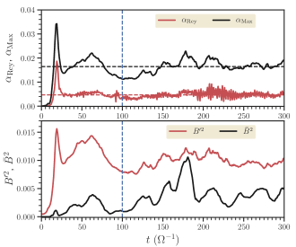
Figure 1: Top panel: Time history of Reynolds ($\alpha_{\rm Rey}$) and Maxwell ($\alpha_{\rm Max}$) stresses. Bottom panel: time history of the volume-averaged mean ($\bar{B}^{2}$) and fluctuating ($B^{\prime 2}$) magnetic energies.

First, consider the time evolution of accretion stresses and magnetic energies. This will also allow us to determine the quasi-stationary phase of the MRI-driven turbulence. The top panel of Fig. 1 shows the time history of accretions stresses (Reynolds and Maxwell). Normalized Reynolds and Maxwell stresses are defined as

$$\alpha_{\rm Rey}=\frac{\langle\overline{\rho v^{\prime}_{x}v^{\prime}_{y}}\rangle}{\langle p_{g}\rangle},$$ (19)

$$\alpha_{\rm Max}=\frac{\langle\bar{B}_{x}\bar{B}_{y}\rangle+\langle\overline{B^{\prime}_{x}B^{\prime}_{y}}\rangle}{\langle p_{g}\rangle},$$ (20)

where the averages are done over the whole volume. Reynolds stress is due to the correlation of fluctuating velocity fields, while Maxwell stress is composed of a correlation between the fluctuating components as well as that between the mean components of the magnetic fields. Both the stresses grow exponentially during the linear regime of MRI, and eventually saturate around an average value when MRI enters into the non-linear regime. In our simulation, we find the time-averaged (within the interval $t=(100-300)\ \Omega^{-1}$) values of Reynolds and Maxwell stresses are to be $\langle\alpha_{\rm Rey}\rangle=0.0048$ and $\langle\alpha_{\rm Max}\rangle=0.0167$ respectively. The ratio of Maxwell to Reynolds stress is $\alpha_{\rm Max}\rangle/\langle\alpha_{\rm Rey}\rangle=3.5$, close to $4$, as predicted by Pessah et al. 2006 for $q=1.5$ and similar to what is found in earlier numerical simulations (Nauman & Blackman 2015; Gressel & Pessah 2015).

The bottom panel of Fig. 1 shows how the volume-averaged mean ($\langle\bar{B}^{2}\rangle$) and fluctuating ($\langle B^{\prime 2}\rangle$) magnetic energies evolve over time. Like accretion stresses, magnetic energies oscillate about an average value in the quasi-stationary phase after the initial exponentially growing phase. It is also worth noting that the mean part of the magnetic field shows a larger time variation than the fluctuating part of the magnetic field. We point out an important point that the fluctuating magnetic field is stronger than the mean magnetic field, and the implication of this will be discussed in the latter part of the paper.

We see in Fig. 1 that the accretion stresses and magnetic energies start saturating around $t=40\ \Omega^{-1}$. However, to remain safer, we consider the simulation in the time range $t=(100-300)\ \Omega^{-1}$ for dynamo coefficient calculation in the quasi-stationary state.

3.2 Evolution of mean fields and EMFs

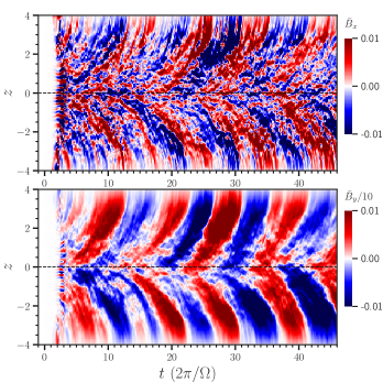
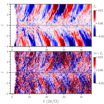
Figure 2: Spatio-temporal variation of mean magnetic fields, $\bar{B}_{x}$ (top left panel), $\bar{B}_{y}$ (bottom left panel) and mean EMFs $\bar{\mathcal{E}}_{x}$ (top right panel) and $\bar{\mathcal{E}}_{y}$ (bottom right panel). Mean magnetic field component $\bar{B}_{y}$ and y-component of EMF $\bar{\mathcal{E}}_{x}$ show a coherent change in space and time (with a time period $\approx 9$ orbital period ($2\pi/\Omega$)), while the spatio-temporal patterns in $\bar{B}_{x}$ and $\bar{\mathcal{E}}_{y}$ are less coherent.

The most preliminary diagnostic of the dynamo is to look at the spatio-temporal variation of the mean magnetic fields, popularly known as the butterfly diagram (e.g. see the review by Brandenburg & Subramanian 2005). Fig. 2 shows the butterfly diagrams for mean magnetic fields $\bar{B}_{x}$ and $\bar{B}_{y}$ along with the mean EMFs $\bar{\mathcal{E}}_{x}$ and $\bar{\mathcal{E}}_{y}$. Here we note that the mean EMF acts as a source term in the mean magnetic field energy evolution equation. In particular, $\bar{\mathcal{E}}_{y}$ is responsible for the generation of poloidal field (here $\bar{B}_{x}$) from a toroidal one due to an $\alpha$-effect, which itself naturally emerges by a combined action of stratification and rotation (Krause & Raedler 1980) in our stratified shearing box simulation. At an early stage of evolution (around $t\approx 2$ orbital period), both mean fields and EMFs show lateral stretches with changing the sign in the vertical direction, which is clearly due to channel modes of MRI (Balbus & Hawley 1992, 1998). During saturation, both mean fields and EMFs show a coherent vertical structure which changes signs in time with a definite period. We find magnetic field components $B_{y}$ and EMF $\bar{\mathcal{E}}_{x}$ show a very coherent spatio-temporal variation with a time period of $\approx 9$ orbital period ($2\pi/\Omega$), similar to the earlier studies of MRI dynamo (Brandenburg et al. 1995; Davis et al. 2010; Gressel 2010; Gressel & Pessah 2015; Ryan et al. 2017). This periodicity is semi-transparent in the butterfly diagram of $\bar{B}_{x}$, while this is hardly apparent for $\bar{\mathcal{E}}_{y}$. However, we note that periodicities exist in all components of mean fields and EMFs as will become clear below (see Fig. 4).

3.3 Evolution of kinetic and current helicities

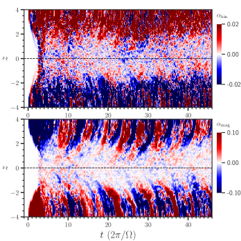
Figure 3: Spatio-temporal variation of $\alpha^{\rm dyn}_{\rm kin}(z,t)$ and $\alpha^{\rm dyn}_{\rm mag}(z,t)$ assuming $\tau_{c}=\Omega^{-1}$. Both the helicities are small close to the mid-plane and become larger at larger heights. The $\alpha_{\rm mag}$ flips sign with a time period $\approx 5$ orbital period ($2\pi/\Omega$), roughly half the dynamo period, while $\alpha_{\rm kin}$ does not show any periodicity.

The generation of large-scale magnetic fields by a dynamo action is often associated with helicity in the fluid velocity field. Assuming isotropic homogeneous turbulence, Krause & Raedler (1980) suggested a kinetic $\alpha$-effect defined by

$$\alpha_{\rm kin}=-\frac{\tau_{c}}{3}\ \overline{v^{\prime}.\nabla\times v^{\prime}}$$ (21)

responsible for magnetic field generation; where $\tau_{c}$ is the correlation time, and $K_{\rm hel}=\overline{v^{\prime}.\nabla\times v^{\prime}}$ is the kinetic helicity. It is suggested that $\alpha_{\rm kin}$ accounting for the effects of the helical velocity field, takes the role of driver, while $\alpha_{\rm mag}$ (Pouquet et al. 1976) defined by

$$\alpha^{\rm dyn}_{\rm mag}(z,t)=\frac{\tau_{c}}{3}\overline{v_{A}^{\prime}.\nabla\times v_{A}^{\prime}},$$ (22)

is the non-linear response arising due to the Lorentz force feedback, gradually increasing and ultimately quenching the kinetic-$\alpha$ (Blackman & Brandenburg 2002; Subramanian 2002). Here, $v^{\prime}_{A}=\sqrt{B^{\prime 2}/\rho}$ is the Alfv̀en velocity and $C_{\rm hel}=\overline{v_{A}^{\prime}.\nabla\times v_{A}^{\prime}}$ is the current helicity. Ideally, the effective $\alpha-$ effect, responsible to poloidal field generation, is supposed to be $\alpha_{\rm dyn}=\alpha_{\rm kin}+\alpha_{\rm mag}$.

Fig. 3 shows the spatio-temporal variation of $\alpha_{\rm kin}$ and $\alpha_{\rm mag}$. We assume $\tau_{c}$ to be same for both $\alpha$-s and $\tau_{c}=\Omega^{-1}$. The $\alpha_{\rm mag}$ changes sign with a time-period $\approx 5$ orbital period ($2\pi/\Omega$), roughly half of the dynamo period, with which the mean fields and EMFs change sign, while $\alpha_{\rm kin}$ does not show any explicit periodicity. We will postpone a detailed discussion on the periodicity of helicities to section 3.5 where we discuss periodicities associated with all important variables.

3.4 Co-existence of small and large scale dynamos

Both kinetic and magnetic-$\alpha$-s are small close to the mid-plane while this is not true of the random kinetic and magnetic energies (see Fig. 6). At the same time, the amplitudes of the helicities increase away from the mid-plane. These features suggest that both small-scale and large-scale dynamo co-exist in MRI-driven dynamo (Blackman & Tan 2004; Gressel 2010). The MRI-driven small-scale dynamo dominates magnetic field generation close to the disc mid-plane (where stratification is unimportant). In contrast, at larger heights where stratification becomes important, a helicity-driven large-scale dynamo governs the magnetic field generation (Dhang & Sharma 2019; Dhang et al. 2020). However, it is to be noted that $\alpha_{\rm mag}$ is larger than $\alpha_{\rm kin}$ by one order of magnitude, and hence it is very likely that the effective-$\alpha$ will be predominantly due to $\alpha_{\rm mag}$.

3.5 Power spectra of mean fields, EMFs and helicities

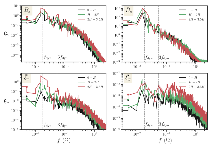
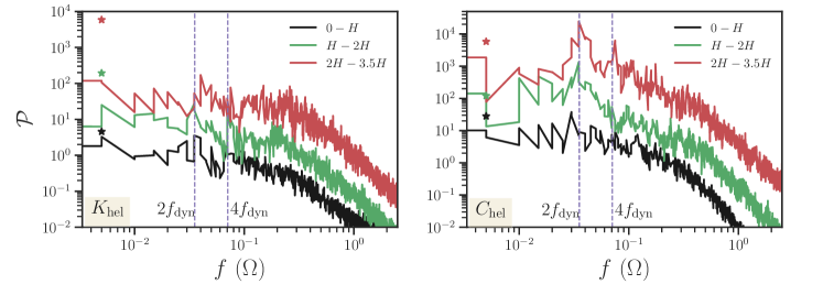
Figure 4: Power spectra of mean fields $\bar{B}_{x}$, $\bar{B}_{y}$ (top panels), mean EMFs $\bar{\mathcal{E}}_{x}$, $\bar{\mathcal{E}}_{y}$ (middle panels) and helicities $K_{\rm hel}$, $C_{\rm hel}$ (bottom panels). Spatial averages are done over different heights: $z=0-H$ (black lines), $z=H-2H$ (green lines), and $z=2H-3.5H$ (red lines). The zeroth frequency values are denoted by ‘asterisks’. Vertical dashed lines denote the dynamo frequency $f_{\rm dyn}=0.017$ and its multiples.

The butterfly diagrams shown in the previous sections depict the apparent periodicities of mean fields, EMFs and helicities. We look at the power spectrum defined by

$$\mathcal{P}_{q}(f)=\frac{1}{z_{2}-z_{1}}\int_{z_{1}}^{z_{2}}dz\ \left|\int\bar{q}(z,t)e^{ift}dt\right|^{2}$$ (23)

where $\bar{q}(z,t)$ is any generic quantity to investigate the periodicities in greater detail. Here the spatial average is done over different heights, namely $z=0-H$, $z=H-2H$ and $z=2H-3.5H$.

Fig. 4 shows the power spectra of mean fields $\bar{B}_{x}$, $\bar{B}_{y}$ (top panels), mean EMFs $\bar{\mathcal{E}}_{x}$, $\bar{\mathcal{E}}_{y}$ (middle panels) and helicities $K_{\rm hel}$, $C_{\rm hel}$ (bottom panels). It is noticeable that power spectra for mean fields and spectra peaks at the primary frequency $f_{\rm dyn}=0.017$, which was also visible in the butterfly diagrams. In addition to the primary frequency, the power spectra also show the presence of higher harmonics (at $3f_{\rm dyn}$), which got unnoticed in the earlier works of MRI dynamo. Similarly, power spectra of current helicity $C_{\rm hel}$ also show the presence of higher harmonics (at $4\ f_{\rm dyn}$) in addition to the primary frequency at $2f_{\rm dyn}$. However, kinetic helicity does not show any periodicity. Presence of a strong time variation in $\alpha_{\rm mag}$ and its dominance over $\alpha_{\rm kin}$ necessarily leads to the expectation that turbulent dynamo coefficients ($\alpha-$ coefficients) should harbour a time-dependent part ($\alpha^{1}_{ij}$) along with the traditional time-independent part ($\alpha^{0}_{ij}$) as discussed in section 4.

4 Results: Dynamo coefficients from IROS

We obtained mean fields ($\bar{B}_{x}$, $\bar{B}_{y}$), EMFs ($\bar{\mathcal{E}}_{x}$, $\bar{\mathcal{E}}_{y}$) from the shearing-box simulation and use a modified version of IROS method (see section 4) to calculate time-independent and time-dependent turbulent dynamo coefficients characterizing the MRI dynamo. However, we find the $x-y$-averaging cannot remove all the signatures of the small-scale dynamo. The small-scale dynamo is expected to have a shorter correlation time of order few $\Omega^{-1}$ and contribute noise at the higher frequency end compared to the large-scale dynamo. Therefore, we further smooth the mean fields and EMFs using a low-pass Fourier filter and remove contributions from the frequencies $f>f_{c}$. We consider three cases: (i) $f_{c}=0.05$ ($\approx 3f_{\rm dyn}$), (ii) $f_{c}=0.12$ ($\approx 6f_{\rm dyn}$) and (iii) $f_{c}\to\infty$ (unfiltered) to assess the effects of the small-scale dynamo on the dynamo coefficient extraction.

4.1 Time independent dynamo coefficients

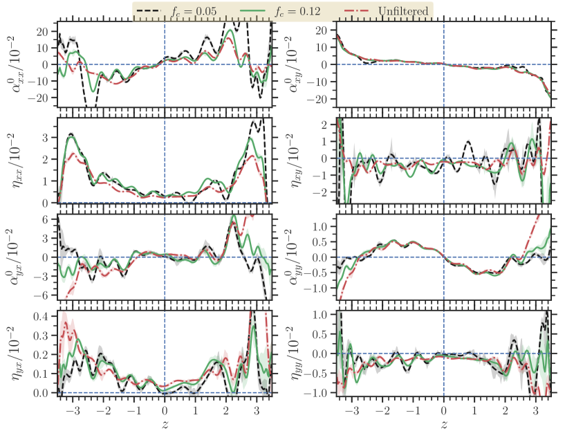
Figure 5: Vertical profiles of time-independent turbulent dynamo coefficients ($\alpha^{0}_{ij}$, $\eta^{0}_{ij}$) in MRI simulation calculated using IROS method. A low-pass Fourier filter with a cut-off frequency $f_{c}$ removes the contribution from the small-scale dynamo. We used two values of $f_{c}$: $f_{c}=0.05$ and $f_{c}=0.12$. The results are compared to the case when IROS is applied to the unfiltered data obtained from DNS.

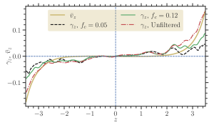
Figure 6: Top panel: profiles of turbulent pumping ($\gamma_{z}$) and mean vertical outflow ($\bar{v}_{z}$). They act in the same direction, transporting mean fields vertically outward. Bottom panel: vertical profiles of average fluctuating velocity ($\overline{v^{\prime 2}}$) and fluctuating Alfven speed $\overline{v^{\prime 2}_{A}}=\overline{B^{\prime 2}}/\overline{\rho}$. Minimal $\tau$ approximation and profiles of $\overline{v^{\prime 2}}$, $\overline{v^{\prime 2}_{A}}$ suggest similar sign of $\gamma_{z}$ as calculated using IROS.

Fig. 5 shows the vertical profiles of time-independent dynamo coefficients $\alpha^{0}_{ij}$ and $\eta_{ij}$ for different values of $f_{c}$. Four panels at the top illustrate the vertical profiles of coefficients ($\alpha^{0}_{xx},\ \alpha^{0}_{xy},\ \eta_{xx},\ \eta_{xy}$) associated with the x-component of EMF $\bar{\mathcal{E}}_{x}$, while four panels at the bottom show profiles of those ($\alpha^{0}_{yx},\ \alpha^{0}_{yy},\ \eta_{yx},\ \eta_{yy}$) associated with the y-component of EMF $\bar{\mathcal{E}}_{y}$.

The ‘coefficient of most interest’ out of the calculated ones is $\alpha^{0}_{yy}$, which plays a vital role in producing the poloidal field (here $\bar{B}_{x}$) out of the toroidal field ($\bar{B}_{y}$) (also see section 4.4). The coefficient $\alpha^{0}_{yy}$ shows an anti-symmetric behaviour about the $z=0$ plane, with a negative (positive) sign in the upper (lower)-half plane (for $|z|<2$). For $|z|>2$, the sign of $\alpha^{0}_{yy}$ tends to be positive (negative) in the upper (lower)-half plane. Earlier studies of MRI dynamo in local (Brandenburg 2008; Gressel 2010; Gressel & Pessah 2015) and global (Dhang et al. 2020) frameworks also found a similar trend in $\alpha^{0}_{yy}$. However, it is to be noted that our study suggests a stronger negative $\alpha^{0}_{yy}$ in the upper-half plane compared to that in the earlier studies. The negative sign in the upper half plane is attributed to the buoyant rise of magnetic flux tubes under the combined action of magnetic buoyancy and shear (Brandenburg & Schmitt 1998; Brandenburg & Subramanian 2005; see also Tharakkal et al. (2023)). Brandenburg & Schmitt (1998) also suggested that negative $\alpha_{yy}$ is responsible for the upward propagation direction of dynamo waves seen in the butterfly diagrams of MRI-driven dynamo simulations (e.g. see Fig. 2). Another different way of looking at the origin of the effective $\alpha$ is to link it to the helicity flux as envisaged by Vishniac 2015 and Gopalakrishnan & Subramanian 2023. We discuss this possibility in section 5.3.

The off-diagonal terms of the $\alpha$-coefficients are related to turbulent pumping. This effect is responsible for transporting large-scale magnetic fields from the turbulent region to the laminar region. We found $\alpha^{0}_{xy}$ and $\alpha^{0}_{yx}$ to be antisymmetric and $\alpha^{0}_{xy}>\alpha^{0}_{yx}$ unlike the previous studies (Brandenburg 2008; Gressel & Pessah 2015) which found $\alpha^{0}_{yx}\approx\alpha^{0}_{xy}$. This resulted in a strong turbulent pumping $\gamma_{z}=(\alpha^{0}_{yx}-\alpha^{0}_{xy})/2$, transporting large-scale magnetic fields from the disc to the corona as shown in the top panel of Fig. 6. We also compare the relative importance of turbulent pumping ($\gamma_{z}$) and wind ($\bar{v}_{z}$) in advecting the magnetic field upward (in the upper half-plane) at different heights. Vertical profiles of $\gamma_{z}$ and $\bar{v}_{z}$ in the top panel of Fig. 6 shows that at low heights ($|z|<2.5$), turbulent pumping is the dominant effect over the wind, while the effects of wind become comparable or larger over the pumping term at large scale-heights (see also Fig. 11).

The theory of isotropic kinematically forced turbulence predicts that $\gamma_{z}$ is supposed to be in the direction of negative gradient of turbulent intensity ($v^{\prime 2}$) (Krause & Raedler 1980), that is, in the negative z-direction (in the upper-half plane) in our simulation. This is opposite to what has been found in Fig. 6. However, it is to be noted that MRI turbulence in a stratified medium is neither isotropic nor homogenous. Minimal $\tau$-approximation (MTA) suggests that in a stratification and rotation-induced anisotropic turbulent medium, which includes the quasi-linear back reaction due to Lorentz forces,

$$\gamma^{\rm MTA}_{z}=-\frac{1}{6}\tau\nabla_{z}(\overline{v^{\prime 2}}-\overline{B^{\prime^{2}}})-\frac{1}{6}\tau^{2}\bf\Omega\hat{z}\times\nabla_{z}(\overline{v^{\prime 2}}+\overline{B^{\prime^{2}}}),$$ (24)

where $\tau$ is the correlation time and it is assumed that $\rho=1$ (see equation (10.59) in Brandenburg & Subramanian 2005). The last term in equation 24 vanishes because all the variables are functions of $z$ alone. Therefore, equation 24 and the bottom panel of Fig. 6 illustrating the vertical profiles of $\overline{v^{\prime 2}}$ and $\overline{v_{A}^{\prime 2}}$ imply that sign of turbulent pumping obtained from MTA supports that obtained from extracted dynamo coefficients.

We found turbulent diffusion tensor $\eta_{ij}$ to be anisotropic with $\eta_{xx}>\eta_{yy}$ and having a significant contribution from the off-diagonal components $\eta_{xy}$ and $\eta_{yx}$. Different values of diagonal components of $\eta_{ij}$ imply that mean field components $\bar{B}_{x}$ and $\bar{B}_{y}$ are affected differently by the vertical diffusion (also see section 4.4). It is worth mentioning that $\eta_{yy}\approx 0$ for the $f_{c}=0.05$ case, while it is slightly negative for the other two cases. This is somewhat different from the earlier studies (Gressel 2010; Gressel & Pessah 2015), which calculated dynamo coefficients using the TF method and found $\eta_{xx}\approx\eta_{yy}>0$. Out of the two off-diagonal terms of the diffusion tensor, $\eta_{yx}$ is of particular interest. It is suggested that a negative value of $\eta_{yx}$ can generate poloidal fields by the shear-current effect (Squire & Bhattacharjee (2016)). However, we find $\eta_{yx}$ to be always positive, nullifying the presence of a shear-current effect in our stratified MRI simulation.

4.2 Time dependent dynamo coefficients

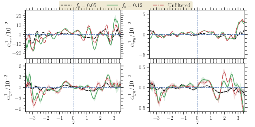
Figure 7: Vertical profiles of time-independent turbulent dynamo coefficients ($\alpha^{1}_{ij}$) in MRI simulation calculated using IROS method. A low-pass Fourier filter with a cut-off frequency $f_{c}$ is used to remove the contribution from the small-scale dynamo. We used two values of $f_{c}$: $f_{c}=0.05$ and $f_{c}=0.12$. The results are compared to the case when IROS is applied to the unfiltered data obtained from DNS.

In the previous sections, We discussed the time-dependent nature of $\alpha_{\rm mag}$. Effective $\alpha$-effect is expected to be determined by $\alpha_{\rm mag}$, especially at the larger scale heights where it is of larger amplitude. While $\alpha$ tensor is expected to have the time-dependent part, $\eta$-tensor is supposed to have only the time-independent part, as it only depends on the turbulent intensity (see section 4). Fig. 7 shows the vertical profiles of components of time-dependent $\alpha$-tensor. We find that $\alpha^{1}_{ij}$-s in the fiducial case ($f_{c}=0.05$) are relatively smaller than the other two cases ($f_{c}=0.12$ and Unfiltered). It is also interesting to note that the coefficients $\alpha_{xx}$ and $\alpha_{yx}$ associated with $\bar{B}_{x}$ in the mean field closure (equation 16) have stronger time-dependence compared to those coefficients ($\alpha_{xy}$ and $\alpha_{yy}$) associated with $\bar{B}_{y}$. Additionally, it is to be noted that the amplitudes of the time-dependent part of $\alpha$-s are higher at larger scale heights. However, overall, the amplitudes of $\alpha^{1}_{ij}$ are much smaller than the $\alpha^{0}_{ij}$ implying that the time-independent $\alpha-$s are predominantly governing the dynamo action.

4.3 Verification of method

To verify the reliability of the determined dynamo coefficients we reconstruct the EMFs using the calculated coefficients and run a 1D dynamo model.

4.3.1 Reconstruction of EMFs

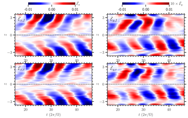
Figure 8: Left panels: Comparison between x-component of EMF $\bar{\mathcal{E}}_{x,f}$ used to determine the turbulent dynamo coefficients,and EMF $\bar{\mathcal{E}}_{x,r}$ reconstructed using the turbulent dynamo coefficients. Right panels: Same as figures in left panels, but for the y-component of EMF.

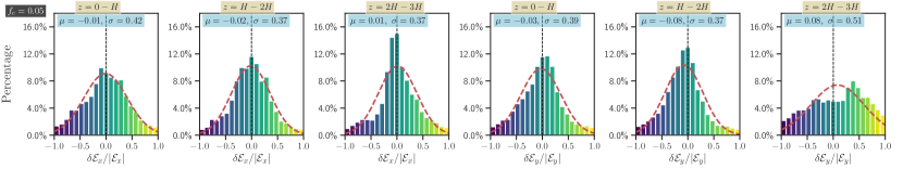
Figure 9: Histograms of the residual EMFs, $\ \delta\bar{\mathcal{E}}_{i}=\bar{\mathcal{E}}_{i,f}-\bar{\mathcal{E}}_{i,r}$ calculated within region of different heights for $f_{c}=0.05$ case. We normalise $\delta\bar{\mathcal{E}}_{i}$ with the absolute values of the corresponding EMFs at the respective points. The Red dashed line shows a normal distribution fitting the histogram.

Fig. 8 shows butterfly diagrams of the EMFs ($\bar{\mathcal{E}}_{x,f},\ \bar{\mathcal{E}}_{y,f}$) used to determine the turbulent dynamo coefficients and the EMFs ($\bar{\mathcal{E}}_{x,r},\ \bar{\mathcal{E}}_{y,r}$) reconstructed using calculated coefficients and mean fields for $f_{c}=0.05$. Here it is to be noted that $\bar{\mathcal{E}}_{x,f},\ \bar{\mathcal{E}}_{y,f}$ are the smoothed EMFs obtained by filtering (by using a low-pass filter) EMFs $\bar{\mathcal{E}}_{x},\ \bar{\mathcal{E}}_{y}$ from DNS respectively. We can see a close match between the broad features, such as the dynamo cycle period, in the smoothed and reconstructed EMFs, implying the goodness of fit.

Further, we investigate the residual of the filtered and reconstructed EMFs, defined by

$$\delta\bar{\mathcal{E}}_{i}=\bar{\mathcal{E}}_{i,f}-\bar{\mathcal{E}}_{i,r},\ \ i\in x,y.$$ (25)

Fig. 9 shows the histograms of the normalised residuals $\delta\bar{\mathcal{E}}_{x}/|\bar{\mathcal{E}}_{x}|$ and $\delta\bar{\mathcal{E}}_{y}/|\bar{\mathcal{E}}_{y}|$ calculated within the region of different heights, namely between $0-H$, $H-2H$ and $2H-3H$, for the $f_{c}=0.05$ case. All the histograms peak about the region close to zero. However, a Gaussian fit of the histograms shows that the mean of the distribution always deviates from zero. Additionally, a careful comparison of histograms of $\delta\bar{\mathcal{E}}_{x}/|\bar{\mathcal{E}}_{x}|$ and $\delta\bar{\mathcal{E}}_{y}/|\bar{\mathcal{E}}_{y}|$ tells that fit is better for $\bar{\mathcal{E}}_{x}$ than that for $\bar{\mathcal{E}}_{y}$, especially at larger scale-heights. Better quality fit for $\bar{\mathcal{E}}_{x}$ over $\bar{\mathcal{E}}_{y}$ is expected as $\bar{\mathcal{E}}_{x}$ obtained from DNS shows a more regular, coherent space-time variation when compared to $\bar{\mathcal{E}}_{y}$.

4.3.2 1D dynamo model

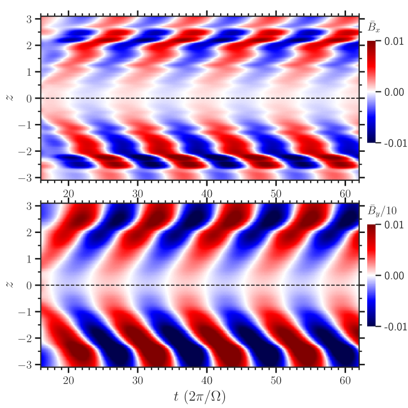
Figure 10: Butterfly diagrams of the mean magnetic fields $\bar{B}_{x}$ and $\bar{B}_{y}$ obtained by running 1D dynamo model. Both $\bar{B}_{x}$ and $\bar{B}_{y}$ flip sign regularly with a cycle of $\approx 9$ orbital period, similar to that found in shearing box simulations (see Fig. 2).

We additionally run a 1D dynamo model using the calculated dynamo coefficients and mean velocity field $\bar{v}_{z}$. In particular we solve equation  13, or in component form

$$\centering\frac{\partial\bar{B}_{x}}{\partial t}\@add@centering =\frac{\partial}{\partial z}\big{[}-(\bar{v}_{z}+\alpha^{0}_{yx})\bar{B}_{x}-\alpha^{0}_{yy}\bar{B}_{y}+\eta_{yy}\frac{\partial\bar{B}_{x}}{\partial z}-\eta_{yx}\frac{\partial\bar{B}_{y}}{\partial z}\big{]}$$

$$\frac{\partial\bar{B}_{y}}{\partial t} =\frac{\partial}{\partial z}\big{[}-(\bar{v}_{z}-\alpha^{0}_{xy})\bar{B}_{y}-\alpha^{0}_{xx}\bar{B}_{x}+\eta_{xx}\frac{\partial\bar{B}_{y}}{\partial z}-\eta_{xy}\frac{\partial\bar{B}_{x}}{\partial z}\big{]}$$

$$+q\Omega\,\bar{B}_{x}.$$ (26)

for $\bar{B}_{x}$ and $\bar{B}_{y}$ with $\alpha^{0}_{ij}$ and $\eta_{ij}$ obtained using the IROS method. We note that $\bar{B}_{z}=0$ as a consequence of the zero net flux (ZNF) assumption in our model. The initial profiles of $\bar{B}_{x}$ and $\bar{B}_{y}$ at are taken directly from the DNS, at time $t=100\Omega^{-1}$ roughly consistent with the beginning of the quasi-stationary phase in the DNS. $\bar{v}_{z}$ profile is taken as a constant throughout the evolution and is also extracted from the direct simulations by averaging it over time throughout the quasi-stationary phase, over which it roughly stays constant. Additionally, for the profiles of dynamo coefficients $\alpha^{0}_{ij}(z)$ and $\eta_{ij}(z)$, we first smooth them with a box filter and also cut them off above and below three scale heights, and use them in the 1D dynamo model. We do this mainly to avoid the instability at boundaries noting that these profiles are sharply flayed outside of that range. Note that only the time independent parts of the dynamo coefficients are used in the mean field equations, since the contributions of $\alpha^{1}_{ij}$ are negligible compared to the time-independent part.

Furthermore, it must be noted that there is a contribution to the diffusion from the mesh grids. We do a rough estimation of numerical diffusion as follows $\eta_{0}=v^{\prime}_{\rm rms}\Delta x$, where we consider the smallest one among the relevant velocities ($v^{\prime}_{\rm rms},\ c_{s},\ v_{A}$) in the problem. Therefore, we add a correction term $\eta_{0}\approx 10^{-3}$ (with $\Delta x=1/32$ and $v^{\prime}_{\rm rms}=0.1$) to the diagonal components of diffusivity tensor $\eta_{ij}$ to consider the contribution from the mesh to the magnetic field diffusion. This also helps us to stabilize the 1D dynamo solution.

With this setup, we solve the system of equations with a finite difference method over a staggered grid of resolution $\Delta z=1/32$, same as the $z$ resolution of DNS. Outcome of this analysis are presented in Fig.  10, where top and bottom panels show the butterfly diagrams of $\bar{B}_{x}$ and $\bar{B}_{y}$ obtained using the 1D dynamo model respectively. We find both x and y-components of mean fields flip sign regularly with a cycle of $\approx 9$ orbital period, similar to what is found in DNS (see Fig. 2). Thus, applying calculated coefficients to the 1D dynamo model successfully reproduces broad features of spatiotemporal variations mean magnetic fields.

4.4 Mean magnetic energy equations

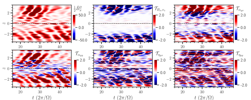
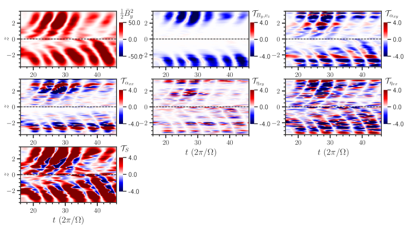
Figure 11: Contributions of different terms involving mean flow ($\bar{v}_{z}$) and turbulent dynamo coefficients ($\alpha_{ij},\ \eta_{ij}$) to the x-(top six panels) and y-(bottom seven panels) components of mean magnetic energy evolution equation (equations 27 and 28). Poloidal field ($\bar{B}_{x}$) generation is primarily attributed to an $\alpha$-effect (the term $\mathcal{T}_{\alpha_{yy}}$), while shear (the term $\mathcal{T}_{\mathcal{S}}$) dominates the toroidal field generation; thus implying and $\alpha-\Omega$ type of dynamo. Winds carry mean fields out of the computational box and contribute largely as the sink term in the mean magnetic energy evolution equation.

It is challenging to calculate dynamo coefficients uniquely in the presence of both shear and rotation (Brandenburg et al. 2008) as there are many unknowns (see also discussion in section 5.4). Therefore, it is worth seeing how different terms involving turbulent dynamo coefficients contribute to the mean magnetic energy equation to make physical sense. The mean magnetic energy evolution equation is obtained by taking the dot product of the mean-field equation (equation 13) with the mean magnetic field $\bf{B}$ and given by

$$\frac{\partial}{\partial t}\left(\frac{1}{2}\bar{B}^{2}_{x}\right) =\mathcal{T}_{B_{x},v_{z}}+\mathcal{T}_{\alpha_{yx}}+\mathcal{T}_{\alpha_{yy}}+\mathcal{T}_{\eta_{yx}}+\mathcal{T}_{\eta_{yy}},$$ (27)

$$\frac{\partial}{\partial t}\left(\frac{1}{2}\bar{B}^{2}_{y}\right) =\mathcal{T}_{B_{y},v_{z}}+\mathcal{T}_{\alpha_{xy}}+\mathcal{T}_{\alpha_{xx}}+\mathcal{T}_{\eta_{xy}}+\mathcal{T}_{\eta_{xx}}+\mathcal{T}_{\mathcal{S}},$$ (28)

where

$$\mathcal{T}_{B_{x},v_{z}} =-\frac{1}{2}\bar{B}_{x}\ \frac{\partial}{\partial z}\left(\bar{v}_{z}\bar{B}_{x}\right),$$ (29)

$$\mathcal{T}_{\alpha_{yx}} =-\frac{1}{2}\bar{B}_{x}\ \frac{\partial}{\partial z}\left(\alpha_{yx}\bar{B}_{x}\right),$$

$$\mathcal{T}_{\alpha_{yy}} =-\frac{1}{2}\bar{B}_{x}\ \frac{\partial}{\partial z}\left(\alpha_{yy}\bar{B}_{y}\right),$$

$$\mathcal{T}_{\eta_{yx}} =-\frac{1}{2}\bar{B}_{x}\ \frac{\partial}{\partial z}\left(\eta_{yx}\frac{\partial}{\partial z}\bar{B}_{y}\right),$$

$$\mathcal{T}_{\eta_{yy}} =\frac{1}{2}\bar{B}_{x}\ \frac{\partial}{\partial z}\left(\eta_{yy}\frac{\partial}{\partial z}\bar{B}_{x}\right),$$

$$\mathcal{T}_{B_{y},v_{z}} =-\frac{1}{2}\bar{B}_{y}\ \frac{\partial}{\partial z}\left(\bar{v}_{z}\bar{B}_{y}\right),$$

$$\mathcal{T}_{\alpha_{xy}} =\frac{1}{2}\bar{B}_{y}\ \frac{\partial}{\partial z}\left(\alpha_{xy}\bar{B}_{y}\right),$$

$$\mathcal{T}_{\alpha_{xx}} =\frac{1}{2}\bar{B}_{y}\ \frac{\partial}{\partial z}\left(\alpha_{xy}\bar{B}_{y}\right),$$

$$\mathcal{T}_{\eta_{xy}} =-\frac{1}{2}\bar{B}_{y}\ \frac{\partial}{\partial z}\left(\eta_{xy}\frac{\partial}{\partial z}\bar{B}_{x}\right),$$

$$\mathcal{T}_{\eta_{xx}} =\frac{1}{2}\bar{B}_{y}\ \frac{\partial}{\partial z}\left(\eta_{xx}\frac{\partial}{\partial z}\bar{B}_{y}\right),$$

$$\mathcal{T}_{\mathcal{S}} =\frac{1}{2}q\Omega\ \bar{B}_{x}\bar{B}_{y}.$$

Fig. 11 shows the space-time plots of different terms involving mean flow ($\bar{v}_{z}$) and turbulent dynamo coefficients ($\alpha_{ij},\ \eta_{ij}$) in the mean magnetic energy evolution equations. The top six panels in Fig. 11 describe the terms in the x-component of the magnetic energy equation (equation 27), while the bottom seven panels illustrate terms in the y-component of the magnetic energy equation ( 28) at different heights and times.

Fig. 11 provides a fairly complicated picture to account for the generation-diffusion scenario of the mean magnetic fields. Broadly speaking, the poloidal field ($\bar{B}_{x}$) is predominantly generated by an $\alpha$-effect (the term $\mathcal{T}_{\alpha_{yy}}$ in Fig. 11). However, there is a significant contribution from $\alpha_{yx}$ (the term $\mathcal{T}_{\alpha_{yx}}$ in Fig. 11) in generating $\bar{B}_{x}$ in larger scale-heights. Toroidal field generation is mainly due to the presence of shear, here differential rotation, ($\mathcal{T}_{\mathcal{S}}$ in Fig. 11) which converts poloidal fields to the toroidal fields. However, it is worth noting that there is a minute contribution from the $\alpha_{xx}$, generating a toroidal field out of the poloidal field by an $\alpha$-effect, (as in an $\alpha^{2}$-$\Omega$ dynamo). The dominance of $\alpha$-effect in generating a poloidal field and that of $\Omega$-effect (shear) in generating a toroidal field imply the presence of an $\alpha-\Omega$ type dynamo in MRI-driven geometrically thin accretion disc. This is similar to what has been found in the study of the dynamo in an MRI-driven geometrically thick accretion disc (Dhang et al. 2020), implying universal action of $\alpha-\Omega$-dynamo in MRI-driven accretion flows.

Generally, it is expected that diagonal components of the diffusion tensor, $\eta_{yy}$ and $\eta_{xx}$ are primarily responsible for the diffusion of $\bar{B}_{x}$ and $\bar{B}_{y}$ respectively. However, our simulation finds that winds carry mean fields out of the computational box and act as a sink in the mean magnetic energy evolution equation, not the $\eta$-s.

5 Discussion

5.1 Periodicities in the dynamo cycle

Investigations of spatio-temporal variation of different variables in our stratified shearing box simulations show a diverse range of periodicities. We observed that mean magnetic fields and EMFs oscillate with a primary frequency $f_{\rm dyn}=0.017$ (equivalent to 9 orbital periods), similar to what was found in earlier studies (Brandenburg et al. 1995; Gammie 1996; Davis et al. 2010; Gressel 2010; Ryan et al. 2017). The primary frequency is determined by the effective dispersion relation of the $\alpha$-$\Omega$ dynamo (Brandenburg & Subramanian 2005; Gressel & Pessah 2015) with the $\alpha$ dominated by the time-independent (DC) value of $\alpha_{yy}$ . The plausible origin of this DC value of $\alpha_{yy}$ is discussed below in section  5.3.

Additionally, we observed the presence of higher harmonics at $3f_{\rm dyn}$, which got unnoticed in earlier MRI simulations (see section 3.5). Unlike the mean fields and EMFs, current helicity shows periodicities at different frequencies $2f_{\rm dyn}$ and $4f_{\rm dyn}$, respectively. The presence of the frequencies in the mean EMFs, mean fields, and current helicities can be understood better if we follow the magnetic helicity density ($h_{b}$) evolution equation (e.g.see Blackman & Field (2000); Subramanian & Brandenburg (2006); Kleeorin & Rogachevskii (2022); Gopalakrishnan & Subramanian (2023)),

$$\frac{1}{2}\frac{\partial h^{b}}{\partial t}=-\bar{\mathcal{E}}.\bar{\bf{B}}-\eta_{0}\mathcal{C}_{\rm hel}-\frac{1}{2}\nabla\cdot\mathcal{F}_{\mathcal{H}},$$ (30)

where $\mathcal{F}_{\mathcal{H}}$ is the helicity flux and the component of the EMF along the mean magnetic field generates mean magnetic and associated current helicities. Now consider the effect of the DC term in $\alpha_{yy}$, which leads to a source $\alpha_{yy}^{0}\bar{B}_{y}^{2}$ in equation 30. This leads to the generation of magnetic and current helicities at a primary frequency, twice that of $\bar{B}_{y}$, i.e. 2 $f_{\rm dyn}$. This current helicity can now add to the $\alpha$-effect, which combined with the mean field in the dynamo equation 13, can lead to secondary EMF and mean fields components oscillating at $3f_{\rm dyn}$ which in turn sources helicity components at $4f_{\rm dyn}$ and so on. These primary and secondary frequency components, limited by noise, are indeed seen from the analysis of our simulations.

5.2 Dynamo coefficients, comparison with earlier studies

Earlier studies calculating turbulent dynamo coefficients using the simulation data and the mean field closure (equation 16) in the local (Brandenburg et al. 1995; Brandenburg 2008; Gressel 2010; Gressel & Pessah 2015; Shi et al. 2016) and global (Flock et al. 2012; Hogg & Reynolds 2018; Dhang & Sharma 2019; Dhang et al. 2020) simulations of MRI-driven accretion discs used different methods. Earlier local (Brandenburg et al. 1995; Davis et al. 2010) and most of the global (Flock et al. 2012; Hogg & Reynolds 2018) studies calculated only the “coefficient of interest” $\alpha_{\phi\phi}$ ($\alpha-$ effect) by neglecting the contributions of other terms in the mean-field closure. Many of the local studies (Brandenburg 2008; Gressel 2010; Gressel & Pessah 2015) use the linear Test Field (TF) method during the run-time to calculate all the coefficients. A few local (e.g. Shi et al. 2016; Zier & Springel 2022; Wissing et al. 2022, the current work) and global (Dhang et al. 2020) studies used direct methods to quantify dynamo coefficients. However, it is important to note that while several authors used a linear regression method assuming few constraints on the diffusion coefficients (namely, $\eta_{xx}=\eta_{yy}$), we use the IROS method without any constrained on the coefficients.

Like most of the earlier local and global studies, we find a negative $\alpha_{yy}$ close to the mid-plane in the upper half-plane. However, direct methods seem to capture negative signs better than TF; which can be realised by comparing $\alpha_{yy}$ profiles in our work (also in Shi et al. (2016)) and in Gressel (2010). Additionally, we find stronger turbulent pumping (compared to that in the TF method), transporting large-scale magnetic fields from the disc to the corona, similar to that found in global MRI-dynamo studies (Dhang et al. 2020).

Additionally, for the first time, we ventured to calculate the time-dependent part of $\alpha_{ij}$ inspired by the periodic behaviour of $\alpha_{\rm mag}$. However, we found that the amplitudes of the time-dependent part of $\alpha-$s ($\alpha^{1}_{ij}$) are much smaller than that of the time-independent $\alpha-$s ($\alpha^{0}_{ij}$). Therefore, we suspect that the time-independent $\alpha-$s are predominantly governing the dynamo action.

Diffusivity coefficients $\eta_{ij}$ in our work are found to be quite different from that in the earlier local studies (Brandenburg 2008; Gressel 2010; Gressel & Pessah 2015; Shi et al. 2016), with $\eta_{xx}\neq\eta_{yy}$ and $\eta_{yy}\approx 0$. Several earlier studies (Shi et al. 2016; Zier & Springel 2022) found $\eta_{yx}<0$) in their unstratified and stratified MRI simulations after imposing a few constraints on the coefficients (e.g. $\eta_{yy}=\eta_{xx},\eta_{xy}=0$ etc.) and they proposed shear-current effect (Raedler, 1980; Rogachevskii & Kleeorin, 2004; Squire & Bhattacharjee, 2016) generating poloidal fields in addition to $\alpha$-effect. Recently, Mondal & Bhat (2023) carried out statistical simulations of MRI in an unstratified ZNF shearing box and found $\eta_{yx}<0$ proposing ‘rotation- shear-current effect’ and the ‘rotation-shear-vorticity effect’ responsible for generating the radial and vertical magnetic fields, respectively. However, like some other studies (TF: Brandenburg 2008; Gressel 2010; Gressel & Pessah 2015), SPH:Wissing et al. 2022), we find $\eta_{yx}\geq 0$, unless we impose a constraint on $\eta_{yy}$ being a positive fraction of $\eta_{xx}$. If we assume $\eta_{yy}=f_{\eta}\ \eta_{xx}$ while calculating the coefficients, we find negativity of $\eta_{yx}$ is an increasing function of the factor $f_{\eta}$ (see Fig. 13 and Appendix). However, we find that the quality of fit is compromised slightly and histograms of the residual of filtered (input) and reconstructed EMFs get broader (with higher standard deviation) with the assumption $\eta_{yy}=f_{\eta}\ \eta_{xx}$. We refer the reader to see Appendix for details.

5.3 Helicity flux and the DC $\alpha-$effect

In order to understand the DC value (time-independent) of the $\alpha$-effect, we take the time average of equation  30. The term $\partial h_{b}/\partial t$ averages to zero, and one gets the well-known constraint (Blackman, 2016; Shukurov & Subramanian, 2021)

$$\langle\bar{\mathcal{E}}\cdot\bar{\bf{B}}\rangle=-\eta_{0}\langle\mathcal{C}_{\rm hel}\rangle-\frac{1}{2}\nabla\cdot\langle\mathcal{F}_{\mathcal{H}}\rangle,$$ (31)

where $\langle\rangle$ indicates a time average. This shows that in the absence of helicity fluxes, the average EMF parallel to the mean field, responsible for the generation of poloidal from the toroidal mean field, is resistively (or catastrophically) quenched. Of the several helicity fluxes discussed in the literature, the generative helicity fluxes as envisaged in Vishniac (2015) and in Gopalakrishnan & Subramanian (2023) can source the DC component of $\bar{\mathcal{E}}\cdot\bar{\bf{B}}$ without the preexistence of any mean field or initial helicities. Using equation (17) of Gopalakrishnan & Subramanian (2023), with mean vorticity $\Omega(2-q)\hat{z}$ and noting that $\alpha_{yy}\bar{B}_{y}^{2}$ dominates $\bar{\mathcal{E}}\cdot\bar{\bf{B}}$, we estimate

$$\begin{split}\left(\alpha_{yy}^{0}\right)_{h_{c}}\approx-\frac{\Omega\tau^{2}}{4\langle\bar{B}_{y}^{2}\rangle}\Bigg{[}\left(C_{1}v_{A}^{\prime 2}+C_{3}v^{\prime 2}+C_{4}\frac{\lambda^{2}}{\tau^{2}}\right)\frac{\partial b^{\prime 2}}{\partial z}\\ +C_{2}b^{\prime 2}\frac{\partial v^{\prime 2}}{\partial z}\Bigg{]},\end{split}$$ (32)

where $(C_{1},C_{2},C_{3},C_{4})=(7/45,-203/5400,403/8100,-1/6)$ and we have taken $q=3/2$. Adopting estimates for the correlation time $\tau\sim\Omega^{-1}$, correlation length $\lambda\sim H/2$ and using the vertical profiles of various physical variables from the simulation, we calculate the vertical profile of $\left(\alpha_{yy}^{0}\right)_{h_{c}}$ due to the generative helicity flux. This is shown as a solid line in Fig.  12 and for comparison, we also show $10\alpha_{yy}^{0}$ (for $f_{c}=0.05$ case) from the IROS inversion. It is encouraging that the $(\alpha_{yy}^{0})_{h_{c}}$ predicted by the generative helicity flux is negative in the north and has a qualitatively similar vertical profile as that determined from IROS inversion. The amplitude, however, is larger, which perhaps indicates the importance also of the neglected diffusive and advective helicity fluxes which act as sink terms in equation 31.

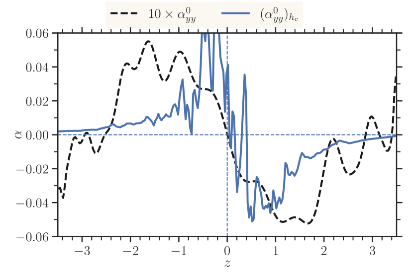
Figure 12: Vertical profiles of $\alpha^{0}_{yy}$ (for $f_{c}=0.05$ case) obtained from IROS inversion and $(\alpha^{0}_{yy})_{h_{c}}$, expected from helicity flux.

5.4 Vanishing $\eta_{yy}$, missing information?

In section 4.4 we pointed out that wind carries away the mean magnetic field and acts as the effective sink of its energy. However, the poloidal field is also expected to be diffused by $\eta_{yy}$, and a positive $\eta_{yy}$ is required for diffusion. Instead, we find a vanishingly small (in some regions even negative) $\eta_{yy}$, which leads us to two possible thoughts: either it is impossible to recover $\eta_{yy}$ in the direct methods, or there is incompleteness in the closure we used to retrieve the coefficients. Here we discuss both possibilities.

It is clear from equation 16 that the turbulent diffusion coefficients are associated with the currents, which are calculated by taking the $z$-derivative of mean magnetic field components. Calculating derivative makes the currents noisy, especially $J_{y}$, as it involves a derivative of $\bar{B}_{x}$, which is fairly incoherent over space and time, as can be seen from the butterfly diagram of $\bar{B}_{x}$ (Fig. 2). Additionally, also note that the $y$-component of EMF is also noisy. Thus, the coefficients associated with $J_{y}$ and $\bar{\mathcal{E}}_{y}$ turned out to be error-prone and difficult to calculate. This pattern has been noticed by earlier works (Squire & Bhattacharjee 2016), which used direct methods other than IROS, used in the current work.

In general, mean EMF can be expressed in terms of symmetric, anti-symmetric tensors and mean fields as follows,

$$\bar{\mathcal{E}}=\tilde{\mathbf{\alpha}}\circ\bar{\mathbf{B}}+\tilde{\mathbf{\gamma}}\times\bar{\mathbf{B}}-\tilde{\mathbf{\eta}}\circ\left(\nabla\times\bar{\mathbf{B}}\right)-\tilde{\mathbf{\delta}}\times\left(\nabla\times\bar{\mathbf{B}}\right)-\tilde{\mathbf{\kappa}}\circ\left(\nabla\bar{\mathbf{B}}\right)^{{\rm sym}},$$ (33)

where we neglect the higher than first-order spatial derivatives and time derivatives of mean fields (Raedler 1980; Brandenburg & Subramanian 2005; Schrinner et al. 2007; Simard et al. 2016). If we define mean fields and EMFs as the $x-y$-averaged quantities, then mean field closure reduces to equation 15. The symmetrised coefficients in equation 33 and non-symmetrised coefficients in equation 15 are related as

$$\tilde{\alpha}_{xx} =\alpha_{xx},$$ (34)

$$\tilde{\alpha}_{yy} =\alpha_{yy},$$

$$\tilde{\gamma}_{z} =\frac{1}{2}\left(\alpha_{yx}-\alpha_{xy}\right),$$

$$\tilde{\eta}_{xx}+\tilde{\kappa}_{xyz} =\eta_{xx},$$

$$\tilde{\eta}_{yy}-\tilde{\kappa}_{yxz} =\eta_{yy},$$

$$\tilde{\delta}_{z} =\frac{1}{2}\left(\eta_{xy}-\eta_{yx}\right)+\frac{1}{2}\left(\tilde{\kappa}_{xxz}+\tilde{\kappa}_{yyz}\right).$$

Therefore it is evident from equation 34 that it is impossible to decouple a few coefficients (coefficients in the last three identities) as there are more unknown coefficients than independent variables ($\bar{\mathbf{B}},\ \bar{\mathcal{E}}$) and the actual diffusion coefficients ($\tilde{\eta}_{ij}$) might be different from the calculated ones ($\eta_{ij}$).

6 Summary

We carried out stratified zero net flux (ZNF) simulations of MRI and characterised the MRI-driven dynamo using the language of mean field dynamo theory. The turbulent dynamo coefficients in the mean-field closure are calculated using the mean magnetic fields and EMFs obtained from the shearing box simulation. For this purpose, we used a cleaning (or inversion) algorithm, namely IROS, adapted to extract the dynamo coefficients. We verified the reliability of extracted coefficients by reconstructing the EMFs and reproducing the cyclic pattern in mean magnetic fields by running a 1D dynamo model. Here we list the key findings of our work:

• We find mean fields and EMFs oscillate with a primary frequency $f_{\rm dyn}=0.017$ ($\approx 9$ orbital period). Additionally, they have higher harmonics at $3f_{\rm dyn}$. Current helicity $\alpha_{\rm mag}$ has two frequencies $2f_{\rm dyn}$ and $4f_{\rm dyn}$ respectively. These frequencies can be understood from mean-field dynamo effective dispersion relation and helicity density evolution equation, respectively (for details, see section 5.1).

• Our unbiased inversion and subsequent analysis show that an $\alpha-$effect ($\alpha_{yy}$) is predominantly responsible for the generation of poloidal field (here $\bar{B}_{x}$) from the toroidal field ($\bar{B}_{y}$). The differential rotation creates a toroidal field from the poloidal field completing the cycle; indicating that an $\alpha-\Omega$-type dynamo is operative in MRI-driven accretion disc.

• We find encouraging evidence that the effective DC $\alpha-$effect can be due to a generative helicity flux (section 5.3).

• We find strong wind ($\bar{v}_{z}$) and turbulent pumping ($\gamma_{z}$) carry out mean fields away from the mid-plane. Interestingly, they act as the principal sink terms in the mean magnetic energy evolution equation instead of the turbulent diffusivity terms.

• The unbiased inversion finds an almost vanishing $\eta_{yy}$, while $\eta_{xx}$ and $\eta_{yx}$ are positive. However $\eta_{yx}$ and $\eta_{yy}$ are strongly correlated; if one imposes an arbitrary prior that $\eta_{yy}=f_{\eta}\eta_{xx}$, then one finds an increasingly negative $\eta_{yx}$ for increasing $f_{\eta}$.

• We point out that defining mean fields by planar averaging can necessarily introduce degeneracy in determining all the turbulent dynamo coefficients uniquely. This may have important consequences for the physical interpretation of the dynamo coefficients.

Data Availability

The data underlying this article will be shared on reasonable request to the corresponding author.

Appendix A Dynamo coefficients with constraints on $\eta_{yy}$

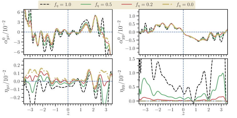
Figure 13: Vertical profiles of the time-independent $\alpha_{ij}$ and $\eta_{ij}$ related to the $\bar{\mathcal{E}}_{y}$ calculated imposing the constraint $\eta_{yy}=\eta_{xx}$ for $f_{c}=0.05$ case. As expected, $\alpha_{ij}$ are not affected with the change in $f_{\eta}$, but $\eta_{ij}$s are. A clear trend has been found; more positive the $\eta_{yy}$ is more negative is $\eta_{yx}$.

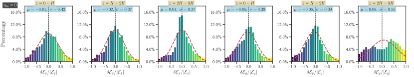
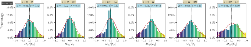
Figure 14: Histograms of the residual EMFs $\delta\bar{\mathcal{E}}_{x}$ (top panels) and $\delta\bar{\mathcal{E}}_{y}$ (bottom panels) for $f_{eta}=0$ and $f_{\eta}=1$. We consider the $f_{c}=0.05$ case. Imposition of constraints on $\eta_{yy}$ compromises the quality of fits, but not significantly because $\alpha_{ij}$ are the main contributors in the fitting of EMFs, not the $\eta_{ij}$.

Diffusivities are challenging to calculate in any direct methods (SVD, linear regression, IROS), as they involve the spatial derivatives of the mean fields. Primarily, we find that $\eta_{yy}$ and $\eta_{xy}$ are noisy as they are related to spatial derivatives of $\bar{B}_{x}$, which is itself quite noisy (e.g. see butterfly diagram in Fig. 2. Some earlier studies (Squire & Bhattacharjee 2016; Shi et al. 2016) put constraints on calculating $\eta$-s, try to alleviate this issue. E.g. Shi et al. (2016) imposed the constraint that $\eta_{yy}=\eta_{xx}$ in the shearing box simulation of MRI and found a negative $\eta_{yx}$, implying the presence of a shear-current effect.

We have, on the other hand, done an unbiased inversion, as it is not clear if such constraints are actually obeyed by MRI-driven turbulence. Nevertheless, for completeness, we explore here a more generalized constraint on $\eta_{yy}$, given by $\eta_{yy}=f_{\eta}\ \eta_{xx}$, and calculate only those coefficients that appear in the mean-field closure for $\bar{\mathcal{E}}_{y}$, as those related to $\bar{\mathcal{E}}_{x}$ remain unaffected. Fig. 13 shows the vertical profiles of $\alpha^{0}_{yx}$, $\alpha^{0}_{yy}$, $\eta_{yx}$ and $\eta_{yy}$ for different values of $f_{\eta}$ and for $f_{c}=0.05$. The coefficients $\alpha_{ij}$ remain almost unaffected, while $\eta_{ij}$ change significantly with change in $f_{\eta}$. There is a clear trend that the more positive the $\eta_{yy}$ (or larger the imposed $f_{\eta}$), the more negative is $\eta_{yx}$. This implies a clear correlation between $\eta_{yx}$ and $\eta_{yy}$.

Further, we investigate the histograms of the residual EMFs $\delta\bar{\mathcal{E}}_{i}$ to check the goodness of the fits. The $x-$components of the residual EMFs remain unaffected as expected, while histograms for $\delta\bar{\mathcal{E}}_{y}$ get slightly broader with the increase in $f_{\eta}$. This implies that the imposition of constraints on $\eta_{yy}$ compromises the quality of fits, but not greatly because $\alpha_{ij}$ are the significant contributors in the fitting of EMFs, not the $\eta_{ij}$.

References

- Bai & Stone (2013) Bai X.-N., Stone J. M., 2013, The Astrophysical Journal, 767, 30
- Balbus & Hawley (1991) Balbus S. A., Hawley J. F., 1991, ApJ, 376, 214
- Balbus & Hawley (1992) Balbus S. A., Hawley J. F., 1992, The Astrophysical Journal, 392, 662
- Balbus & Hawley (1998) Balbus S. A., Hawley J. F., 1998, Reviews of Modern Physics, 70, 1
- Beckwith et al. (2011) Beckwith K., Armitage P. J., Simon J. B., 2011, MNRAS, 416, 361
- Begelman & Armitage (2023) Begelman M. C., Armitage P. J., 2023, MNRAS, 521, 5952
- Bendre et al. (2020) Bendre A. B., Subramanian K., Elstner D., Gressel O., 2020, MNRAS, 491, 3870
- Bendre et al. (2023) Bendre A. B., Schober J., Dhang P., Subramanian K., 2023, arXiv e-prints, p. arXiv:2308.00059
- Bhat et al. (2016) Bhat P., Ebrahimi F., Blackman E. G., 2016, Monthly Notices of the Royal Astronomical Society, 462, 818
- Blackman (2016) Blackman E. G., 2016, in Balogh A., Bykov A., Eastwood J., Kaastra J., eds, , Vol. 51, Multi-scale Structure Formation and Dynamics in Cosmic Plasmas. pp 59–91, doi:10.1007/978-1-4939-3547-5_3
- Blackman & Brandenburg (2002) Blackman E. G., Brandenburg A., 2002, ApJ, 579, 359
- Blackman & Field (2000) Blackman E. G., Field G. B., 2000, ApJ, 534, 984
- Blackman & Tan (2004) Blackman E. G., Tan J. C., 2004, Ap&SS, 292, 395
- Bodo et al. (2011) Bodo G., Cattaneo F., Ferrari A., Mignone A., Rossi P., 2011, ApJ, 739, 82
- Bodo et al. (2014) Bodo G., Cattaneo F., Mignone A., Rossi P., 2014, ApJ, 787, L13
- Brandenburg (2008) Brandenburg A., 2008, Astronomische Nachrichten, 329, 725
- Brandenburg & Donner (1997) Brandenburg A., Donner K. J., 1997, MNRAS, 288, L29
- Brandenburg & Schmitt (1998) Brandenburg A., Schmitt D., 1998, A&A, 338, L55
- Brandenburg & Subramanian (2005) Brandenburg A., Subramanian K., 2005, Phys. Rep., 417, 1
- Brandenburg et al. (1995) Brandenburg A., Nordlund A., Stein R. F., Torkelsson U., 1995, ApJ, 446, 741
- Brandenburg et al. (2008) Brandenburg A., Rädler K. H., Rheinhardt M., Käpylä P. J., 2008, ApJ, 676, 740
- Chandrasekhar (1960) Chandrasekhar S., 1960, Proceedings of the National Academy of Sciences, 46, 253
- Coleman et al. (2017) Coleman M. S. B., Yerger E., Blaes O., Salvesen G., Hirose S., 2017, MNRAS, 467, 2625
- Davis et al. (2010) Davis S. W., Stone J. M., Pessah M. E., 2010, ApJ, 713, 52
- Dhang & Sharma (2019) Dhang P., Sharma P., 2019, MNRAS, 482, 848
- Dhang et al. (2020) Dhang P., Bendre A., Sharma P., Subramanian K., 2020, MNRAS, 494, 4854
- Dhang et al. (2023) Dhang P., Bai X.-N., White C. J., 2023, ApJ, 944, 182
- Flock et al. (2012) Flock M., Dzyurkevich N., Klahr H., Turner N., Henning T., 2012, ApJ, 744, 144
- Fromang & Papaloizou (2007) Fromang S., Papaloizou J., 2007, A&A, 476, 1113
- Gammie (1996) Gammie C. F., 1996, ApJ, 457, 355
- Gardiner & Stone (2005) Gardiner T. A., Stone J. M., 2005, Journal of Computational Physics, 205, 509
- Goldreich & Lynden-Bell (1965) Goldreich P., Lynden-Bell D., 1965, MNRAS, 130, 125
- Gopalakrishnan & Subramanian (2023) Gopalakrishnan K., Subramanian K., 2023, ApJ, 943, 66
- Gressel (2010) Gressel O., 2010, MNRAS, 405, 41
- Gressel & Pessah (2015) Gressel O., Pessah M. E., 2015, ApJ, 810, 59
- Gressel & Pessah (2022) Gressel O., Pessah M. E., 2022, ApJ, 928, 118
- Guan & Gammie (2011) Guan X., Gammie C. F., 2011, ApJ, 728, 130
- Guan et al. (2009) Guan X., Gammie C. F., Simon J. B., Johnson B. M., 2009, ApJ, 694, 1010
- Hammersley et al. (1992) Hammersley A., Ponman T., Skinner G., 1992, Nuclear Instruments and Methods in Physics Research A, 311, 585
- Hawley (2001) Hawley J. F., 2001, ApJ, 554, 534
- Hawley et al. (1995) Hawley J. F., Gammie C. F., Balbus S. A., 1995, ApJ, 440, 742
- Hawley et al. (2013) Hawley J. F., Richers S. A., Guan X., Krolik J. H., 2013, ApJ, 772, 102
- Hirose et al. (2014) Hirose S., Blaes O., Krolik J. H., Coleman M. S. B., Sano T., 2014, ApJ, 787, 1
- Högbom (1974) Högbom J. A., 1974, A&AS, 15, 417
- Hogg & Reynolds (2016) Hogg J. D., Reynolds C. S., 2016, ApJ, 826, 40
- Hogg & Reynolds (2018) Hogg J. D., Reynolds C. S., 2018, ApJ, 861, 24
- Johansen et al. (2009) Johansen A., Youdin A., Klahr H., 2009, ApJ, 697, 1269
- Kleeorin & Rogachevskii (2022) Kleeorin N., Rogachevskii I., 2022, MNRAS, 515, 5437
- Krause & Raedler (1980) Krause F., Raedler K. H., 1980, Mean-field magnetohydrodynamics and dynamo theory
- Lesur & Ogilvie (2008) Lesur G., Ogilvie G. I., 2008, A&A, 488, 451
- Mattia & Fendt (2022) Mattia G., Fendt C., 2022, ApJ, 935, 22
- Mignone et al. (2007) Mignone A., Bodo G., Massaglia S., Matsakos T., Tesileanu O., Zanni C., Ferrari A., 2007, ApJS, 170, 228
- Miyoshi & Kusano (2005) Miyoshi T., Kusano K., 2005, Journal of Computational Physics, 208, 315
- Mondal & Bhat (2023) Mondal T., Bhat P., 2023, arXiv e-prints, p. arXiv:2307.01281
- Nauman & Blackman (2015) Nauman F., Blackman E. G., 2015, MNRAS, 446, 2102
- Parkin & Bicknell (2013) Parkin E. R., Bicknell G. V., 2013, MNRAS, 435, 2281
- Pessah et al. (2006) Pessah M. E., Chan C.-K., Psaltis D., 2006, Physical Review Letters, 97, 221103
- Pessah et al. (2007) Pessah M. E., Chan C.-k., Psaltis D., 2007, ApJ, 668, L51
- Pouquet et al. (1976) Pouquet A., Frisch U., Leorat J., 1976, Journal of Fluid Mechanics, 77, 321
- Raedler (1980) Raedler K. H., 1980, Astronomische Nachrichten, 301, 101
- Riols et al. (2013) Riols A., Rincon F., Cossu C., Lesur G., Longaretti P. Y., Ogilvie G. I., Herault J., 2013, Journal of Fluid Mechanics, 731, 1
- Rogachevskii & Kleeorin (2004) Rogachevskii I., Kleeorin N., 2004, Phys. Rev. E, 70, 046310
- Ryan et al. (2017) Ryan B. R., Gammie C. F., Fromang S., Kestener P., 2017, ApJ, 840, 6
- Salvesen et al. (2016) Salvesen G., Simon J. B., Armitage P. J., Begelman M. C., 2016, MNRAS, 457, 857
- Schekochihin et al. (2005) Schekochihin A. A., Haugen N. E. L., Brandenburg A., Cowley S. C., Maron J. L., McWilliams J. C., 2005, ApJ, 625, L115
- Schrinner et al. (2007) Schrinner M., Rädler K.-H., Schmitt D., Rheinhardt M., Christensen U. R., 2007, Geophysical and Astrophysical Fluid Dynamics, 101, 81
- Shi et al. (2010) Shi J., Krolik J. H., Hirose S., 2010, ApJ, 708, 1716
- Shi et al. (2016) Shi J.-M., Stone J. M., Huang C. X., 2016, MNRAS, 456, 2273
- Shukurov & Subramanian (2021) Shukurov A., Subramanian K., 2021, Astrophysical Magnetic Fields: From Galaxies to the Early Universe. Cambridge Astrophysics, Cambridge University Press, doi:10.1017/9781139046657
- Simard et al. (2016) Simard C., Charbonneau P., Dubé C., 2016, Advances in Space Research, 58, 1522
- Simon et al. (2009) Simon J. B., Hawley J. F., Beckwith K., 2009, ApJ, 690, 974
- Simon et al. (2012) Simon J. B., Beckwith K., Armitage P. J., 2012, MNRAS, 422, 2685
- Squire & Bhattacharjee (2016) Squire J., Bhattacharjee A., 2016, Journal of Plasma Physics, 82, 535820201
- Stepanovs et al. (2014) Stepanovs D., Fendt C., Sheikhnezami S., 2014, ApJ, 796, 29
- Stone et al. (1999) Stone J. M., Pringle J. E., Begelman M. C., 1999, MNRAS, 310, 1002
- Subramanian (2002) Subramanian K., 2002, Bulletin of the Astronomical Society of India, 30, 715
- Subramanian & Brandenburg (2006) Subramanian K., Brandenburg A., 2006, ApJL, 648, L71
- Tharakkal et al. (2023) Tharakkal D., Shukurov A., Gent F. A., Sarson G. R., Snodin A., 2023, arXiv e-prints, p. arXiv:2305.03318
- Velikhov (1959) Velikhov E., 1959, Sov. Phys. JETP, 36, 995
- Vishniac (2015) Vishniac E. T., 2015, in American Astronomical Society Meeting Abstracts #225. p. 229.08
- Wissing et al. (2022) Wissing R., Shen S., Wadsley J., Quinn T., 2022, A&A, 659, A91
- Zier & Springel (2022) Zier O., Springel V., 2022, MNRAS, 517, 2639
- von Rekowski et al. (2003) von Rekowski B., Brandenburg A., Dobler W., Dobler W., Shukurov A., 2003, A&A, 398, 825