11institutetext: Physik-Institut, Universität Zürich, Winterthurerstrasse 190, 8057 Zürich, Switzerland22institutetext: Institut für Theoretische Physik, Universität Regensburg, 93040 Regensburg, Germany33institutetext: Department of Physics and Astronomy, Michigan State University, East Lansing, MI 48824, USA

Complete $N_{f}^{2}$ contributions to four-loop pure-singlet splitting functions

Thomas Gehrmann thomas.gehrmann@uzh.ch 2, 3    Andreas von Manteuffel manteuffel@ur.de 1    Vasily Sotnikov vasily.sotnikov@physik.uzh.ch 1, 3    Tong-Zhi Yang toyang@physik.uzh.ch
Abstract

The scale evolution of parton distributions is determined by universal splitting functions. As a milestone towards the computation of these functions to four-loop order in QCD, we compute all contributions to the pure-singlet quark-quark splitting functions that involve two closed fermion loops. The splitting functions are extracted from the pole terms of off-shell operator matrix elements, and the workflow for their calculation is outlined. We reproduce known results for the non-singlet four-loop splitting functions and validate our new pure-singlet results against fixed Mellin moments.

Keywords:
QCD, Multi-loop Amplitudes, Deep Inelastic Scattering, Operator Product Expansion
preprint: MSUHEP-23-024, ZU-TH 43/23

1 Introduction

The parton distribution functions are universal ingredients to the theory prediction of any collider observable that involves hadrons in the initial state. Their scale evolution Altarelli:1977zs ; Gribov:1972ri ; Dokshitzer:1977sg is governed by splitting functions, which can be determined order-by-order in perturbative QCD. Complete analytic expressions for the splitting functions are available up to three loops in QCD Altarelli:1977zs ; Gross:1974cs ; Floratos:1978ny ; Gonzalez-Arroyo:1979qht ; Curci:1980uw ; Furmanski:1980cm ; Moch:2004pa ; Vogt:2004mw .

To enable consistent predictions for collider observables, a matching level of precision is required among the hard subprocess cross sections and the parton evolution: NLO QCD predictions involve parton distributions evolved according to the two-loop splitting functions and NNLO QCD implies three-loop evolution. Following pioneering results on the Higgs and Drell-Yan cross sections Anastasiou:2015vya ; Mistlberger:2018etf ; Duhr:2020seh , an increasing number of N3LO calculations for benchmark collider processes is now being accomplished (see e.g. Heinrich:2020ybq for a recent review). These highlight the urgent need for four-loop parton evolution. Partial results at four loops were obtained for parts of the non-singlet splitting functions Moch:2017uml and for a finite number of Mellin moments of the singlet splitting functions Moch:2021qrk ; Falcioni:2023luc ; Falcioni:2023vqq . This information on the four-loop splitting functions could already be used to approximate N3LO-accurate parton distributions McGowan:2022nag ; Hekhorn:2023gul . The computation of the full set of the four-loop splitting functions remains an outstanding task, required to enable fully consistent hadron collider predictions at N3LO accuracy.

In this paper, we employ the framework for computing the splitting functions from the divergences of massless off-shell operator matrix elements (OMEs). This technique is based on the operator product expansion (OPE) and has been applied successfully in splitting function calculations at lower loop orders Gross:1974cs ; Floratos:1978ny ; Gonzalez-Arroyo:1979qht ; Hamberg:1991qt ; Blumlein:2021enk ; Blumlein:2021ryt ; Gehrmann:2023ksf . Compared to the extraction of splitting functions from physical subprocess coefficient functions Moch:2004pa ; Vogt:2004mw , the OPE-based approach is particularly attractive, since it typically leads to simpler types of Feynman amplitudes and Feynman integrals. However, the off-shell nature of the operator matrix elements gives rise to a complicated mixing between the physical operators and unphysical gauge-variant operators under renormalization Dixon:1974ss ; Kluberg-Stern:1974iel ; Collins:1994ee ; Falcioni:2022fdm .

In this paper, we describe the calculation of all contributions with two closed fermion loops to the pure-singlet splitting functions at four loops, using the OPE technique. To determine the renormalization counterterms resulting from these gauge-variant operators we follow the novel procedure proposed by some of us in Gehrmann:2023ksf , which is summarized in Section 2. The computation of OMEs to four-loop order is described in Section 3. This workflow is then applied in Section 4 to obtain the results for the complete four-loop $N_{f}^{2}$ contributions to the pure-singlet splitting functions and to confirm previous results for the $N_{f}^{2}$ contributions to the non-singlet splitting functions. We conclude with an outlook in Section 5.

2 Renormalization of the twist-two operators

To study the collinear behavior of QCD at leading power, we consider the twist-two operators from the operator product expansion. With regards to the flavor group, the twist-two operators are decomposed into non-singlet and singlet parts. The non-singlet operators of spin $n$ are given by

$$O^{\mu_{1}\cdots\mu_{n}}_{q,k}=\frac{i^{n-1}}{2}\mathcal{S}\bigg{[}\bar{\psi}_{i_{1}}\gamma^{\mu_{1}}D^{\mu_{2}}_{i_{1}i_{2}}D^{\mu_{3}}_{i_{2}i_{3}}\cdots D^{\mu_{n}}_{i_{n-1}i_{n}}\,\frac{\lambda_{k}}{2}\psi_{i_{n}}-\text{trace terms}\bigg{]},\,k=3,\cdots N_{f}^{2}-1\,,$$ (1)

while the two singlet quark and gluon operators are

$\displaystyle O^{\mu_{1}\cdots\mu_{n}}_{q}$ $\displaystyle=\frac{i^{n-1}}{2}\mathcal{S}\bigg{[}\bar{\psi}_{i_{1}}\gamma^{\mu_{1}}D^{\mu_{2}}_{i_{1}i_{2}}D^{\mu_{3}}_{i_{2}i_{3}}\cdots D^{\mu_{n}}_{i_{n-1}i_{n}}\psi_{i_{n}}-\text{trace terms}\bigg{]}\,,$
$\displaystyle O^{\mu_{1}\cdots\mu_{n}}_{g}$ $\displaystyle=-\frac{i^{n-2}}{2}\mathcal{S}\bigg{[}G^{\mu_{1}}_{a_{1},\mu}D^{\mu_{2}}_{a_{1}a_{2}}\cdots D^{\mu_{n-1}}_{a_{n-2}a_{n-1}}G^{\mu_{n}\mu}_{a_{n-1}a_{n}}-\text{trace terms}\bigg{]}\,,$ (2)

where $\mathcal{S}$ denotes symmetrization of Lorentz indices $\mu_{1}\cdots\mu_{n}$ and $\lambda_{k}/2$ are diagonal generators of the flavor group $\text{SU}(N_{f})$. In the above equations, $\psi$ and $G_{\mu\nu}^{a}$ represent the quark field and gluon field strength tensor, respectively, and $D^{\mu}=\partial_{\mu}-ig_{s}\textbf{T}^{a}A^{a}_{\mu}$ is the covariant derivative in either the fundamental or the adjoint representation of a general gauge group. In this paper, we consider only the operators associated with zero-momentum transfer.

In practice, it is convenient to extract the information of interest by contracting the above operators with a fully symmetric external source $J_{\mu_{1}\cdots\mu_{n}}=\Delta_{\mu_{1}}\Delta_{\mu_{2}}\cdots\Delta_{\mu_{n}}$, where $\Delta$ is light-like with $\Delta^{2}=0$. In this way, we define the following spin-$n$ operators,

$\displaystyle O_{q,k}$ $\displaystyle=O^{\mu_{1}\cdots\mu_{n}}_{q,k}J_{\mu_{1}\cdots\mu_{n}}\,,$
$\displaystyle O_{q}$ $\displaystyle=O^{\mu_{1}\cdots\mu_{n}}_{q}J_{\mu_{1}\cdots\mu_{n}}\,,$
$\displaystyle O_{g}$ $\displaystyle=O^{\mu_{1}\cdots\mu_{n}}_{g}J_{\mu_{1}\cdots\mu_{n}}\,.$ (3)

As usual, the non-singlet operator is renormalized multiplicatively, i.e.,

$$O^{\text{R}}_{q,k}=Z_{\text{ns}}O^{\text{B}}_{q,k}\,,$$ (4)

where here and below we introduce the superscript R and B to denote the renormalized and bare operators, respectively.

However, for singlet operators, in addition to mixing among themselves under renormalization, they also mix with other unphysical operators, the so-called gauge-variant (GV) operators. This mixing was first pointed out by Gross and Wilczek in the first extraction of the one-loop singlet anomalous dimensions Gross:1974cs . Subsequently, the renormalization of twist-two operators and the theory of the renormalization of a general gauge-invariant operator have been widely studied in the literature, by the seminal works of Dixon and Taylor Dixon:1974ss , Kluberg-Stern and Zuber Kluberg-Stern:1974nmx ; Kluberg-Stern:1975ebk , Joglekar and Lee Joglekar:1975nu , Collins and Scalise Collins:1994ee . These works allowed explicit derivations of the GV operators at order $g_{s}$ and enabled the extraction of the correct anomalous dimension to two loops Hamberg:1991qt , thereby resolving earlier inconsistencies between different groups Floratos:1978ny ; Gonzalez-Arroyo:1979qht . However, it is not clear how to generalize those works to enable the construction of the GV operators beyond order $g_{s}$. Recently, starting from a generalized gauge symmetry and promoting it to a generalized BRST symmetry, Falcioni and Herzog Falcioni:2022fdm were able to construct the GV operators for fixed $n$ to higher orders.

A general framework has been formulated to derive the renormalization counterterms resulting from the GV operators with all-$n$ dependence Gehrmann:2023ksf . For completeness, we describe this framework briefly below, the details can be found in Gehrmann:2023ksf . The framework generalizes the naive renormalization

$\displaystyle\left(\begin{array}[]{c}O_{q}\\ O_{g}\end{array}\right)^{\text{R,naive}}=\left(\begin{array}[]{cc}Z_{qq}&Z_{qg}\\ Z_{gq}&Z_{gg}\end{array}\right)\left(\begin{array}[]{c}O_{q}\\ O_{g}\end{array}\right)^{\text{B}}\,$ (11)

to

$\displaystyle\left(\begin{array}[]{c}O_{q}\\ O_{g}\\ O_{ABC}\\ \end{array}\right)^{\text{R}}=\left(\begin{array}[]{ccc}Z_{qq}&Z_{qg}&Z_{qA}\\ Z_{gq}&Z_{gg}&Z_{gA}\\ 0&0&Z_{AA}\\ \end{array}\right)\left(\begin{array}[]{c}O_{q}\\ O_{g}\\ O_{ABC}\\ \end{array}\right)^{\text{B}}+\left(\begin{array}[]{c}\left[ZO\right]_{q}^{\textrm{GV}}\\ \left[ZO\right]_{g}^{\textrm{GV}}\\ \left[ZO\right]_{A}^{\textrm{GV}}\end{array}\right)^{\text{B}}\,,$ (24)

where we introduce GV operator $O_{ABC}=O_{A}+O_{B}+O_{C}$ with $O_{A},\,O_{B},\,O_{C}$ denoting the gluon, quark, and ghost GV operators respectively. As discussed in Gehrmann:2023ksf , the GV operator $O_{ABC}$ alone is insufficient for renormalizing the physical operators $O_{q}$ and $O_{g}$. Additional terms are necessary, denoted in the above equation as $\left[ZO\right]_{q}^{\textrm{GV}}$, $\left[ZO\right]_{g}^{\textrm{GV}}$, and $\left[ZO\right]_{A}^{\textrm{GV}}$, where $Z$ and $O$ are written together. This notation is used because it becomes impractical to disentangle the renormalization constants from their associated operators while retaining the complete dependence on all powers of $n$. Thus, the renormalization constants here should be distinguished from those appearing in the first term on the right-hand side of the above equation. Notice that these additional terms are GV counterterms for the purpose of canceling the non-physical contributions only. Thus it is not necessary for the above equation to exhibit the pattern of multiplicative renormalization. In addition to the physical renormalization constants $Z_{ij}$ with $i,j=q,g$, we also introduce non-physical renormalization constants $Z_{qA},Z_{gA},Z_{AA}$ associated with GV operators $O_{ABC}$. These non-physical renormalization constants and GV counterterms only start to contribute from a certain order in $a_{s}=g_{s}^{2}/(4\pi)^{2}$, specifically:

$\displaystyle Z_{qA}$ $\displaystyle=\mathcal{O}(a_{s}^{2}),\,$ $\displaystyle\qquad\left[ZO\right]_{q}^{\textrm{GV}}$ $\displaystyle=\mathcal{O}(a_{s}^{3})\,,$
$\displaystyle Z_{gA}$ $\displaystyle=\mathcal{O}(a_{s}),\,$ $\displaystyle\left[ZO\right]_{g}^{\textrm{GV}}$ $\displaystyle=\mathcal{O}(a_{s}^{2})\,,$ (25)

Our strategy Gehrmann:2023ksf is to explicitly extract the counterterm Feynman rules associated to the GV operators instead of determining the GV operators themselves. The strategy relies on considering multi-leg, off-shell operator matrix elements (OMEs), which are defined as the Green’s functions or matrix elements with an operator insertion. For example, in the two-point case we have,

$\displaystyle A_{ij}=\braket{j(p)}{O_{i}}{j(p)}\text{ with }p^{2}<0\,,$ (26)

where $O_{i}$ represents a twist-two operator and $j$ with momentum $p$ denotes a quark, gluon or ghost external state. The established framework is valid to all orders in $g_{s}$ and we have worked out in Gehrmann:2023ksf the Feynman rules for $O_{ABC}$ to order $g_{s}^{2}$ as well as the counterterm Feynman rules for $\left[ZO\right]_{g}^{\textrm{GV}}$ to order $a_{s}^{2}\,g_{s}$, where $a_{s}$ and $g_{s}$ stemming from $Z$ and $O$ respectively. These counterterm Feynman rules are enough to extract physical renormalization constants as well as $Z_{qA},\,Z_{gA}$ to three-loop order. As we will see below, the counterterm Feynman rules derived in Gehrmann:2023ksf are sufficient to determine $Z_{qq}$ to four-loop order.

To extract $Z_{qq}$, we only need to consider the renormalization of $O_{q}$,

$\displaystyle O^{\text{R}}_{q}$ $\displaystyle=$ $\displaystyle Z_{qq}O^{\text{B}}_{q}+Z_{qg}O^{\text{B}}_{g}+Z_{qA}O^{\text{B}}_{ABC}+\left[ZO\right]_{q}^{\textrm{GV}}\,.$ (27)

Inserting the above equations into two-quark external states, we obtain

$\displaystyle\braket{q}{O^{\text{R}}_{q}}{q}$ $\displaystyle=Z_{q}\bigg{[}Z_{qq}\braket{q}{O^{\text{B}}_{q}}{q}$
$\displaystyle+Z_{qg}\braket{q}{O^{\text{B}}_{g}}{q}+Z_{qA}\braket{q}{O^{\text{B}}_{ABC}}{q}+\braket{q}{\left[ZO\right]_{q}^{\textrm{GV}}}{q}\bigg{]}\bigg{|}_{a_{s}^{\text{B}}\to Z_{a_{s}}a_{s},\,\xi^{\text{B}}\to Z_{g}\xi}\,,$ (28)

where we introduced the quark and gluon wave function renormalization constants $Z_{q}$, $Z_{g}$, and the strong coupling renormalization constant $Z_{a_{s}}$. Explicit expressions for them are collected in appendix A. Further, $\xi$ is the gauge parameter, where $\xi=1$ corresponds to Feynman gauge.

For the determination of $Z_{qq}$ at four loops, we need to compute the OME $\braket{q}{O^{\text{B}}_{q}}{q}$ to four-loop order, which will be described in detail in Section 3 below. In addition we use the known results for OMEs $\braket{q}{O^{\text{B}}_{g}}{q}$ and $\braket{q}{O^{\text{B}}_{ABC}}{q}$ up to three-loop and two-loop orders respectively Gehrmann:2023ksf . Lastly, the OME $\braket{q}{\left[ZO\right]_{q}^{\textrm{GV}}}{q}$ needs to be evaluated to four-loop order. It was shown in the appendix of Gehrmann:2023ksf , that the counterterm Feynman rules for the $qq$, $gg$ and $qqg$ vertices resulting from $\left[ZO\right]_{q}^{\textrm{GV}}$ are zero, which leads to the following conclusion:

$$\braket{q}{\left[ZO\right]_{q}^{\textrm{GV}}}{q}=\mathcal{O}(a_{s}^{5})\,.$$ (29)

The renormalization constants above satisfy the renormalization group equations

$$\frac{dZ}{d\ln\mu}=-2\gamma\cdot Z\,.$$ (30)

In the non-singlet case, the anomalous dimension can be extracted from $Z_{\text{ns}}$ by solving (30) with the help of the $d$-dimensional QCD $\beta$ function

$\displaystyle\beta(a_{s},\,\epsilon)=\frac{da_{s}}{d\ln\mu}=-2\epsilon\,a_{s}-2a_{s}\sum_{i=0}^{\infty}a_{s}^{i+1}\beta_{i}\,,$ (31)

where $\epsilon=(4-d)/2$. Explicitly, we have,

$\displaystyle Z_{\text{ns}}=$ $\displaystyle 1+a_{s}\frac{\gamma^{(0)}_{\text{ns}}}{\epsilon}+a_{s}^{2}\Bigg{(}\frac{\gamma_{\text{ns}}^{(1)}}{2\epsilon}+\frac{1}{2\epsilon^{2}}\bigg{[}-\beta_{0}\gamma_{\text{ns}}^{(0)}+\big{(}\gamma_{\text{ns}}^{(0)}\big{)}^{2}\bigg{]}\Bigg{)}$
$\displaystyle+a_{s}^{3}\Bigg{(}\frac{1}{3\epsilon}\gamma_{\text{ns}}^{(2)}+\frac{1}{6\epsilon^{2}}\bigg{[}-2\beta_{1}\gamma_{\text{ns}}^{(0)}-2\beta_{0}\gamma_{\text{ns}}^{(1)}+3\gamma^{(0)}_{\text{ns}}\gamma^{(1)}_{\text{ns}}\bigg{]}$
$\displaystyle\quad+\frac{1}{6\epsilon^{3}}\bigg{[}2\beta_{0}^{2}\gamma_{\text{ns}}^{(0)}-3\beta_{0}\big{(}\gamma_{\text{ns}}^{(0)}\big{)}^{2}+\big{(}\gamma_{\text{ns}}^{(0)}\big{)}^{3}\bigg{]}\Bigg{)}$
$\displaystyle+\frac{a_{s}^{4}}{24}\Bigg{(}\frac{1}{\epsilon^{4}}\bigg{[}-6\beta_{0}^{3}\gamma_{\text{ns}}^{(0)}-6\beta_{0}(\gamma_{\text{ns}}^{(0)})^{3}+11\beta_{0}^{2}(\gamma_{\text{ns}}^{(0)})^{2}+(\gamma_{\text{ns}}^{(0)})^{4}\bigg{]}$
$\displaystyle\quad+\frac{1}{\epsilon^{3}}\bigg{[}{6\beta_{0}^{2}\gamma_{\text{ns}}^{(1)}-14\beta_{0}\gamma_{\text{ns}}^{(0)}\gamma_{\text{ns}}^{(1)}+12\beta_{0}\beta_{1}\gamma_{\text{ns}}^{(0)}+6\gamma_{\text{ns}}^{(1)}(\gamma_{\text{ns}}^{(0)})^{2}-8\beta_{1}(\gamma_{\text{ns}}^{(0)})^{2}}{}\bigg{]}$
$\displaystyle\quad+\frac{1}{\epsilon^{2}}\bigg{[}{-6\beta_{0}\gamma_{\text{ns}}^{(2)}-6\beta_{1}\gamma_{\text{ns}}^{(1)}-6\beta_{2}\gamma_{\text{ns}}^{(0)}+8\gamma_{\text{ns}}^{(0)}\gamma_{\text{ns}}^{(2)}+3(\gamma_{\text{ns}}^{(1)})^{2}}{}\bigg{]}+\frac{6\gamma_{\text{ns}}^{(3)}}{\epsilon}\Bigg{)}$
$\displaystyle+\mathcal{O}(a_{s}^{5})\,.$ (32)

The non-singlet anomalous dimension $\gamma_{\text{ns}}$ can be decomposed into the following form by separating the even and odd moments,

$\displaystyle\gamma_{\text{ns}}=\frac{1+(-1)^{n}}{2}\gamma_{\text{ns}}^{+}+\frac{1-(-1)^{n}}{2}\left(\gamma_{\text{ns}}^{-}+\gamma^{\text{s}}_{\text{ns}}\right),$ (33)

where the detailed definitions of $\gamma_{\text{ns}}^{\pm}$ and $\gamma_{\text{ns}}^{\text{s}}$ can be found, for example, in Moch:2004pa . Here and in the rest of this paper, we always expand the anomalous dimension according to

$$\gamma=\sum_{l=1}^{\infty}a_{s}^{l}\gamma^{(l-1)}\,,$$ (34)

while for the renormalization constants we follow a different convention,

$$Z=\sum_{l=0}^{\infty}a_{s}^{l}Z^{(l)}\,.$$ (35)

In the singlet case, our goal is the determination of the physical anomalous dimensions $\gamma_{ij}$. They can be read off from the physical renormalization constants $Z_{ij}$,

$\displaystyle Z_{ij}=$ $\displaystyle+\delta_{ij}+a_{s}\frac{\gamma^{(0)}_{ij}}{\epsilon}+a_{s}^{2}\Bigg{(}\frac{\gamma_{ij}^{(1)}}{2\epsilon}+\frac{1}{2\epsilon^{2}}\bigg{[}-\beta_{0}\gamma_{ij}^{(0)}+\sum_{k=q,\,g}\gamma^{(0)}_{ik}\gamma^{(0)}_{kj}\bigg{]}\Bigg{)}$
$\displaystyle+a_{s}^{3}\Bigg{(}\frac{1}{3\epsilon}\gamma_{ij}^{(2)}+\frac{1}{6\epsilon^{2}}\bigg{[}-2\beta_{1}\gamma_{ij}^{(0)}-2\beta_{0}\gamma_{ij}^{(1)}+2\sum_{k=q,\,g}\gamma^{(1)}_{ik}\gamma^{(0)}_{kj}+\sum_{k}\gamma^{(0)}_{ik}\gamma^{(1)}_{kj}\bigg{]}$
$\displaystyle\quad+\frac{1}{6\epsilon^{3}}\bigg{[}2\beta_{0}^{2}\gamma_{ij}^{(0)}-3\beta_{0}\sum_{k=q,\,g}\gamma_{ik}^{(0)}\gamma_{kj}^{(0)}+\sum_{k=q,\,g}\sum_{l=q,\,g}\gamma^{(0)}_{ik}\gamma^{(0)}_{kl}\gamma^{(0)}_{lj}\bigg{]}\Bigg{)}$
$\displaystyle+\frac{a_{s}^{4}}{24}\Bigg{(}\frac{1}{\epsilon^{4}}\bigg{[}11\beta_{0}^{2}\sum_{k=q,\,g}\gamma^{(0)}_{ik}\gamma^{(0)}_{kj}-6\beta_{0}\sum_{k=q,\,g}\sum_{l=q,\,g}\gamma^{(0)}_{ik}\gamma^{(0)}_{kl}\gamma^{(0)}_{lj}$
$\displaystyle\quad+\sum_{k=q,\,g}\sum_{l=q,\,g}\sum_{m=q,\,g}\gamma^{(0)}_{ik}\gamma^{(0)}_{kl}\gamma^{(0)}_{lm}\gamma^{(0)}_{mj}-6\beta_{0}^{3}\gamma^{(0)}_{ij}\bigg{]}+\frac{1}{{\epsilon^{3}}}\bigg{[}-5\beta_{0}\sum_{k=q,\,g}\gamma^{(0)}_{ik}\gamma^{(1)}_{kj}$
$\displaystyle\quad-9\beta_{0}\sum_{k=q,\,g}\gamma^{(1)}_{ik}\gamma^{(0)}_{kj}-8\beta_{1}\sum_{k=q,\,g}\gamma^{(0)}_{ik}\gamma^{(0)}_{kj}+\sum_{k=q,\,g}\sum_{l=q,\,g}\gamma^{(0)}_{ik}\gamma^{(0)}_{kl}\gamma^{(1)}_{lj}$
$\displaystyle\quad+2\sum_{k=q,\,g}\sum_{l=q,\,g}\gamma^{(0)}_{ik}\gamma^{(1)}_{kl}\gamma^{(0)}_{lj}+3\sum_{k=q,\,g}\sum_{l=q,\,g}\gamma^{(1)}_{ik}\gamma^{(0)}_{kl}\gamma^{(0)}_{lj}+6\beta_{0}^{2}\gamma^{(1)}_{ij}+12\beta_{1}\beta_{0}\gamma^{(0)}_{ij}\bigg{]}$
$\displaystyle\quad+\frac{1}{\epsilon^{2}}\bigg{[}2\sum_{k=q,\,g}\gamma^{(0)}_{ik}\gamma^{(2)}_{kj}+3\sum_{k=q,\,g}\gamma^{(1)}_{ik}\gamma^{(1)}_{kj}+6\sum_{k}\gamma^{(2)}_{ik}\gamma^{(0)}_{kj}-6\beta_{2}\gamma^{(0)}_{ij}$
$\displaystyle\quad-6\beta_{1}\gamma^{(1)}_{ij}-6\beta_{0}\gamma^{(2)}_{ij}{}\bigg{]}+\frac{6\gamma^{(3)}_{ij}}{\epsilon}\Bigg{)}+\mathcal{O}(a_{s}^{5})\,,$ (36)

where $i,j=q,g$. Notice that if we consider only $q$ instead of $g$ for the dummy indices $k,l,m$ in the above summations, the above equation has the same form as the equation (2). Furthermore, equation (2) remains unaltered even when GV operators (counterterms) are introduced. This is due to the fact that the renormalization of GV operators (counterterms) does not involve mixing with the physical operators, as demonstrated in Joglekar:1975nu . In other words, the mixing matrix in (24) has a block-triangular form. In this paper, we are mainly interested in the $N_{f}^{2}$ contributions to both, the non-singlet anomalous dimension $\gamma^{(3)}_{\text{ns}}$ and the pure-singlet anomalous dimension $\gamma^{(3)}_{\text{ps}}$ defined by

$$\gamma^{(3)}_{\text{ps}}=\gamma^{(3)}_{qq}-\gamma^{+,(3)}_{\text{ns}}\,,$$ (37)

where $N_{f}$ is the number of massless quark flavors.

3 Computational method

As demonstrated above, for the purpose of extracting $Z_{qq}$ at the four-loop order, the last missing contribution is the OME $\braket{q}{O^{\text{B}}_{q}}{q}$ at four loops. In this section, we focus on the computation of the $N_{f}^{2}$ part for this OME. The corresponding Feynman diagrams were generated by QGRAF Nogueira:1991ex , see Fig. 1 for some sample Feynman diagrams. The required Feynman rules in $n$-space involve non-standard terms like $(\Delta\cdot p)^{n-1}$ and are not convenient for the application of integration-by-parts (IBP) reductions Chetyrkin:1981qh ; Tkachov:1981wb ; Laporta:2000dsw . To overcome this problem, a method first proposed in Ablinger:2012qm ; Ablinger:2014nga is adopted. The method sums the non-standard terms into linear propagators depending on a tracing parameter $t$. For example,

$\displaystyle(\Delta\cdot p)^{n-1}\to\sum_{n=1}^{\infty}(\Delta\cdot p)^{n-1}t^{n}=\frac{t}{1-t\Delta\cdot p}\,.$ (38)

In the following, we always work in parameter-$t$ space, which allows us to use standard IBP algorithms. To generate the unreduced amplitude in parameter-$t$ space, Mathematica is used to substitute the Feynman rules into the Feynman diagrams generated by QGRAF Nogueira:1991ex and FORM Vermaseren:2000nd is used to deal with the Dirac and color algebra. To reduce the size of the raw amplitude, we first classify the diagrams into different integral families with an in-house code invoking Reduze 2 vonManteuffel:2012np and FeynCalc Shtabovenko:2016sxi ; Shtabovenko:2021hjx . During the family classification, partial fractions among the Feynman propagators are needed, especially for the linear propagators, and Apart Feng:2012iq is used for this task. At later stages of the calculation, we also use MultivariateApart Heller:2021qkz to decompose rational functions of kinematic invariants and parameters into multivariate partial fractions (see also Pak:2011xt ; Bendle:2021ueg ; Gerlach:2022qnc for alternative decompositions).

Refer to caption
Refer to caption
Figure 1: Representative Feynman diagrams for $N_{f}^{2}$ contributions to the OME $\braket{q}{O^{\text{B}}_{q}}{q}$ at four loops. The first diagram contributes to the non-singlet anomalous dimension, while the second diagram contributes to the pure-singlet anomalous dimension in the quark channel.

To reduce the amplitude and to calculate the master integrals in the differential equation approach Gehrmann:1999as , we perform IBP reductions of the four-loop integrals using finite field sampling and rational reconstruction vonManteuffel:2014ixa ; Peraro:2016wsq ; Peraro:2019svx . An optimized input system of equations is prepared by employing the method of Agarwal:2020dye to control the generation of squared propagators. We note that the unreduced amplitude contains not only irreducible numerators but also higher powers of the propagators, in particular for the linear ones. For the computation of the reductions, we group integrals into so-called sectors, which label different sets of denominators. For each sector, we generate IBP identities by constructing suitable differential operators and subsequently applying them to so-called seed integrals which have positive powers of the denominators of the sector. We eliminate redundant equations from the system for each sector, where for performance reasons we ignore relations which involve only integrals in sub-sectors, that is, with fewer different denominators. It is well known that ignoring subsector information in this way can lead to incomplete reductions, since one misses specific relations, which are sometimes referred to as “hidden” or “anomalous”. In the present case, we recover such relations from differential equations and dimensional analysis, as will be explained below. The private code Finred is used to perform the filtering as well as the final reduction including also all subsector integrals.

We compute the differential equations for the master integrals chosen through a generic integral ordering (see e.g. vonManteuffel:2012np ) by a straight-forward IBP reduction of their derivatives. Here, we compute the derivatives both with respect to $t$ and $p^{2}$. In dimensional regularization, one can derive a relation between the partial derivatives from the behavior of the integral under a rescaling of all dimensionful parameters (see e.g. Abreu:2022mfk ). We observe that some of them are not manifestly fulfilled, which we interpret as a consequence of incomplete reductions due to missing “hidden” relations. By enforcing these scaling relations, we obtain a number of additional identities, which relate integrals from different sectors with the same number of different propagators (and subsector integrals). These additional relations simplify the differential equations in $t$ for the remaining master integrals and we cast them into $\epsilon$-form Henn:2013pwa using the codes CANONICA Meyer:2016slj ; Meyer:2017joq and Libra Lee:2014ioa ; Lee:2020zfb . We obtain

$$\mathrm{d}\vec{I}(t,\epsilon)=\epsilon\sum_{i}\mathrm{d}\ln(t-t_{i})\mathbf{A}^{\!(i)}\vec{I}(t,\epsilon)\,,$$ (39)

where we have set $p^{2}=-1$ and $\Delta\cdot p=1$. $\vec{I}$ is the vector of the new basis integrals, $\mathbf{A}^{\!(i)}$ are matrices of rational numbers and $t_{i}=0,\pm 1$.

Integrals without any $t$-dependent linear propagators are standard four-loop self-energy integrals Baikov:2010hf ; Lee:2011jt , which in the present case were mapped to the planar two-point functions in vonManteuffel:2019gpr . We use these integrals to determine the purely $\epsilon$-dependent prefactors needed to transition from a basis in $\epsilon$-form to a basis with uniformly transcendental (UT) solutions. In addition, they provide all the explicit boundary conditions that we need in addition to the following structural requirement. Due to the fact that we introduce $t$ as a tracing parameter for a power series about $t=0$ and that our transformations of the integral coefficient are rational, the solutions of interest should have no branch cuts. We take thus the limit $t\to 0$, solve the differential equation for exact $\epsilon$ and require the absence of branch cuts. This gives additional conditions we can impose on our $\epsilon$-expanded solutions with exact $t$ dependence in the limit $t\to 0$. In this way, we solve our master integrals as a Laurent expansion in $\epsilon$, where the coefficients are UT combinations of harmonic polylogarithms (HPLs) Remiddi:1999ew with weights $0,\pm 1$ and argument $t$ as well as zeta values.

We reduce the amplitude in terms of UT integrals and reconstruct the $d$ dependence as well as the $t$ dependence of the coefficients for a given finite field. Here, we take advantage of the anticipated factorization of denominators and first determine the denominators Abreu:2018zmy ; Heller:2021qkz (as well as some simple overall numerator factors) in order to simplify the multivariate reconstruction. We insert the $\epsilon$-expanded solutions for the master integrals into the amplitude and find the poles of the bare amplitude to contain transcendental functions of up to weight 7. It is at this level of the $\epsilon$-expanded bare amplitude that we reconstruct the rational numbers from their image in a single finite field of cardinality $\mathcal{O}(2^{63})$. A second finite field is used to check the reconstruction.

The result for the $N_{f}^{2}$ part of the bare four-loop OME $\braket{q}{O^{\text{B}}_{q}}{q}$ is then given in parameter-$t$ space. It is transformed to $n$-space in terms of harmonic sums Vermaseren:1998uu ; Blumlein:1998if with the help of the package HarmonicSums Ablinger:2009ovq ; Ablinger:2012ufz ; Ablinger:2014rba ; Ablinger:2011te ; Ablinger:2013cf ; Ablinger:2014bra , yielding the $n$-space expression for the bare OME.

4 Renormalization and results

With the four-loop results for the bare OME computed in the above section in hand, all ingredients required for the renormalization procedure in (2) are now available. We notice that the non-physical renormalization constant $Z_{qA}$ needs to be evaluated to three loops and the three-loop corrections of $\braket{q}{O^{\text{B}}_{q}}{q}$ need to be obtained to finite terms in $\epsilon$. Both of them were already obtained previously Gehrmann:2023ksf . Combining all components according to (2), the $N_{f}^{2}$ part of $Z_{qq}$ is determined to four-loop order and the corresponding anomalous dimension can be easily extracted from (2). Similarly, the $N_{f}^{2}$ contributions for non-singlet anomalous dimensions are determined through (4) and (2) and cross-checked against the results provided in Davies:2016jie . We do not repeat them here and restrict ourselves to displaying the new results for the pure-singlet anomalous dimension in $n$-space. We find:

$\displaystyle\gamma^{(3)}_{\text{ps}}$ $\displaystyle(n)\big{|}_{C_{F}N_{f}^{3}}=\frac{16\left(n^{2}+n+2\right)^{2}}{9(n-1)n^{2}(n+1)^{2}(n+2)}\left(6\zeta_{3}-4S_{1,1,1}\right)$
$\displaystyle+\frac{64\left(8n^{7}+37n^{6}+83n^{5}+85n^{4}+61n^{3}+58n^{2}-20n-24\right)S_{1,1}}{27(n-1)n^{3}(n+1)^{3}(n+2)^{2}}$
$\displaystyle-\frac{32}{81(n-1)n^{4}(n+1)^{4}(n+2)^{3}}\bigg{[}64n^{10}+464n^{9}+1449n^{8}+2037n^{7}+1012n^{6}$
$\displaystyle+105n^{5}-411n^{4}-1784n^{3}-1304n^{2}-48n+144\bigg{]}S_{1}+\frac{16}{81(n-1)n^{5}(n+1)^{5}(n+2)^{4}}\bigg{[}$
$\displaystyle 64n^{13}+576n^{12}+2168n^{11}+3376n^{10}+258n^{9}-4248n^{8}-3615n^{7}-4520n^{6}$
$\displaystyle-7225n^{5}-1722n^{4}+3304n^{3}+1840n^{2}-336n-288\bigg{]}\,,$ (40)
$\displaystyle\gamma^{(3)}_{\text{ps}}$ $\displaystyle(n)\big{|}_{C_{F}^{2}N_{f}^{2}}=\frac{1}{81(n-1)^{2}n^{7}(n+1)^{7}(n+2)^{5}}\bigg{[}5413n^{19}+57482n^{18}+254354n^{17}$
$\displaystyle+639426n^{16}+1396536n^{15}+4120966n^{14}+11962810n^{13}+25755742n^{12}$
$\displaystyle+38724195n^{11}+32487128n^{10}-11246124n^{9}-77944456n^{8}-127667936n^{7}$
$\displaystyle-142086912n^{6}-123597440n^{5}-83330816n^{4}-43996416n^{3}-18487296n^{2}$
$\displaystyle-5557248n-829440\bigg{]}-\frac{256\left(n^{2}+n+2\right)^{2}S_{-3}}{3(n-1)^{2}n^{3}(n+1)^{3}(n+2)^{2}}$
$\displaystyle-\frac{32\left(n^{9}+6n^{8}+14n^{7}+40n^{6}+137n^{5}+506n^{4}+784n^{3}+672n^{2}+560n+224\right)S_{-2}}{3(n-1)^{2}n^{4}(n+1)^{4}(n+2)^{3}}$
$\displaystyle-\frac{4}{81(n-1)n^{5}(n+1)^{5}(n+2)^{4}}\bigg{[}6895n^{13}+68895n^{12}+296692n^{11}+703266n^{10}$
$\displaystyle+1104101n^{9}+1623673n^{8}+2693912n^{7}+3944838n^{6}+4420952n^{5}+3670248n^{4}$
$\displaystyle+2067520n^{3}+699296n^{2}+91776n-8064\bigg{]}S_{1}+\frac{8}{81(n-1)n^{4}(n+1)^{4}(n+2)^{2}}\bigg{[}655n^{9}$
$\displaystyle+4026n^{8}+8100n^{7}-5502n^{6}-38027n^{5}-67940n^{4}-80336n^{3}-56704n^{2}-20112n$
$\displaystyle-2880\bigg{]}S_{2}$
$\displaystyle+\frac{32\left(77n^{8}+284n^{7}+433n^{6}-31n^{5}-312n^{4}-93n^{3}-498n^{2}+260n+456\right)S_{3}}{27(n-1)^{2}n^{3}(n+1)^{3}(n+2)^{2}}$
$\displaystyle-\frac{32\left(23n^{8}+86n^{7}+217n^{6}+461n^{5}+270n^{4}-99n^{3}-18n^{2}-52n+264\right)\zeta_{3}}{9(n-1)^{2}n^{3}(n+1)^{3}(n+2)^{2}}$
$\displaystyle+\frac{8}{81(n-1)n^{4}(n+1)^{4}(n+2)^{3}}\bigg{[}2501n^{10}+18325n^{9}+57780n^{8}+96942n^{7}$
$\displaystyle+120281n^{6}+181533n^{5}+246102n^{4}+221096n^{3}+156608n^{2}+77328n+19296\bigg{]}S_{1,1}$
$\displaystyle-\frac{16\left(5n^{7}+19n^{6}-409n^{5}-2675n^{4}-4388n^{3}-3896n^{2}-2912n-816\right)S_{1,2}}{27(n-1)n^{3}(n+1)^{3}(n+2)^{2}}$
$\displaystyle-\frac{16\left(91n^{7}+425n^{6}+661n^{5}-721n^{4}-2152n^{3}-2080n^{2}-2224n-816\right)S_{2,1}}{27(n-1)n^{3}(n+1)^{3}(n+2)^{2}}$
$\displaystyle-\frac{8\left(n^{2}+n+2\right)\left(133n^{4}+226n^{3}+457n^{2}+284n+4\right)S_{1,1,1}}{9(n-1)n^{3}(n+1)^{3}(n+2)}$
$\displaystyle+\frac{16\left(n^{2}+n+2\right)^{2}}{9(n-1)n^{2}(n+1)^{2}(n+2)}\bigg{(}45\zeta_{4}-16S_{4}-12S_{1}\zeta_{3}-8S_{1,3}+2S_{2,2}-4S_{3,1}$
$\displaystyle-6S_{1,1,2}+2S_{1,2,1}+14S_{2,1,1}+22S_{1,1,1,1}\bigg{)}\,,$ (41)
$\displaystyle\gamma^{(3)}_{\text{ps}}$ $\displaystyle(n)\big{|}_{C_{F}C_{A}N_{f}^{2}}=-\frac{4}{81(n-2)(n-1)^{2}n^{5}(n+1)^{6}(n+2)^{5}}\bigg{[}7627n^{17}+74941n^{16}$
$\displaystyle+279109n^{15}+298173n^{14}-931399n^{13}-3113931n^{12}-2639893n^{11}+1581811n^{10}$
$\displaystyle+4213772n^{9}+2908014n^{8}+1843168n^{7}+3691920n^{6}+7684032n^{5}+11725312n^{4}$
$\displaystyle+12278016n^{3}+7778304n^{2}+2654208n+373248\bigg{]}$
$\displaystyle+\frac{16\left(n^{2}+n+2\right)\left(5n^{2}+5n+6\right)S_{-4}}{3(n-1)n^{2}(n+1)^{2}(n+2)}$
$\displaystyle-\frac{16\left(59n^{8}+224n^{7}+489n^{6}+765n^{5}+174n^{4}-565n^{3}-742n^{2}-556n-232\right)S_{-3}}{9(n-1)^{2}n^{3}(n+1)^{3}(n+2)^{2}}$
$\displaystyle+\frac{8}{81(n-2)(n-1)^{2}n^{4}(n+1)^{4}(n+2)^{3}}\bigg{[}209n^{12}-389n^{11}-380n^{10}-10012n^{9}$
$\displaystyle-20569n^{8}+24309n^{7}+68716n^{6}+129788n^{5}+109304n^{4}-126512n^{3}-190400n^{2}$
$\displaystyle-109632n-33408\bigg{]}S_{-2}+\frac{4}{81(n-1)^{2}n^{5}(n+1)^{5}(n+2)^{4}}\bigg{[}9353n^{14}+87430n^{13}$
$\displaystyle+345549n^{12}+674794n^{11}+510973n^{10}-273064n^{9}-781035n^{8}-890768n^{7}$
$\displaystyle-1217312n^{6}-1089848n^{5}-309768n^{4}+26496n^{3}-132544n^{2}-117888n-21888\bigg{]}S_{1}$
$\displaystyle+\frac{8}{81(n-1)^{2}n^{4}(n+1)^{4}(n+2)^{3}}\bigg{[}59n^{11}-205n^{10}+1091n^{9}+6453n^{8}+10481n^{7}$
$\displaystyle+11791n^{6}-4815n^{5}-39715n^{4}-37428n^{3}-13424n^{2}-2688n-720\bigg{]}S_{2}$
$\displaystyle-\frac{8\left(367n^{8}+1342n^{7}+2387n^{6}+1195n^{5}-192n^{4}-297n^{3}-3870n^{2}-380n+1752\right)S_{3}}{27(n-1)^{2}n^{3}(n+1)^{3}(n+2)^{2}}$
$\displaystyle+\frac{16\left(n^{2}+n+2\right)\left(23n^{2}+23n+34\right)S_{4}}{9(n-1)n^{2}(n+1)^{2}(n+2)}$
$\displaystyle+\frac{32\left(7n^{8}+29n^{7}+69n^{6}+147n^{5}+94n^{4}-36n^{3}+18n^{2}-32n+88\right)\zeta_{3}}{3(n-1)^{2}n^{3}(n+1)^{3}(n+2)^{2}}$
$\displaystyle+\frac{16\left(n^{2}+n+2\right)\left(23n^{2}+23n+22\right)S_{-3,1}}{9(n-1)n^{2}(n+1)^{2}(n+2)}-\frac{64\left(n^{2}+n-10\right)\left(n^{2}+n+2\right)S_{-2,-2}}{9(n-1)n^{2}(n+1)^{2}(n+2)}$
$\displaystyle+\frac{32\left(71n^{7}+367n^{6}+866n^{5}+1609n^{4}+1657n^{3}+994n^{2}+892n+360\right)S_{-2,1}}{27(n-1)n^{3}(n+1)^{3}(n+2)^{2}}$
$\displaystyle+\frac{32\left(n^{2}+n+2\right)\left(7n^{2}+7n+2\right)S_{-2,2}}{9(n-1)n^{2}(n+1)^{2}(n+2)}+\frac{128\left(n^{2}+n+1\right)\left(n^{2}+n+2\right)S_{1,-3}}{3(n-1)n^{2}(n+1)^{2}(n+2)}$
$\displaystyle-\frac{64\left(52n^{7}+224n^{6}+541n^{5}+554n^{4}+317n^{3}+164n^{2}-460n-288\right)S_{1,-2}}{27(n-1)n^{3}(n+1)^{3}(n+2)^{2}}$
$\displaystyle-\frac{16}{81(n-1)^{2}n^{4}(n+1)^{4}(n+2)^{3}}\bigg{[}1474n^{11}+9886n^{10}+28861n^{9}+43998n^{8}$
$\displaystyle+35410n^{7}+22892n^{6}+8871n^{5}-36800n^{4}-46032n^{3}-3040n^{2}+11664n+2304\bigg{]}S_{1,1}$
$\displaystyle-\frac{16\left(n^{2}+n+2\right)\left(40n^{5}+138n^{4}+325n^{3}+471n^{2}+190n+24\right)S_{1,2}}{9(n-1)n^{3}(n+1)^{3}(n+2)^{2}}$
$\displaystyle+\frac{16\left(n^{2}+n+2\right)\left(5n^{2}+5n+14\right)S_{1,3}}{3(n-1)n^{2}(n+1)^{2}(n+2)}$
$\displaystyle+\frac{16\left(n^{2}+n+2\right)\left(16n^{6}+66n^{5}-87n^{4}-158n^{3}-43n^{2}-58n-24\right)S_{2,1}}{27(n-1)^{2}n^{3}(n+1)^{3}(n+2)^{2}}$
$\displaystyle-\frac{32\left(n^{2}+n+2\right)\left(19n^{2}+19n-10\right)S_{-2,1,1}}{9(n-1)n^{2}(n+1)^{2}(n+2)}-\frac{64\left(n^{2}+n-10\right)\left(n^{2}+n+2\right)S_{1,-2,1}}{9(n-1)n^{2}(n+1)^{2}(n+2)}$
$\displaystyle+\frac{32\left(n^{2}+n+2\right)\left(38n^{5}+39n^{4}+86n^{3}+29n^{2}-78n-26\right)S_{1,1,1}}{9(n-1)^{2}n^{3}(n+1)^{3}(n+2)}$
$\displaystyle+\frac{16\left(n^{2}+n+2\right)^{2}}{9(n-1)n^{2}(n+1)^{2}(n+2)}\bigg{(}-45\zeta_{4}-6S_{2,-2}-8S_{2,2}+15S_{3,1}+44S_{1,1,-2}$
$\displaystyle+29S_{1,1,2}+15S_{1,2,1}+2S_{2,1,1}-22S_{1,1,1,1}\bigg{)}\,,$ (42)

where we omit the argument $n$ of the harmonic sums defined by

$\displaystyle S_{\pm m_{1},\,m_{2},\,\cdots m_{d}}(n)$ $\displaystyle=\sum_{j=1}^{n}(\pm 1)^{j}j^{-m_{1}}S_{m_{2},\,\cdots m_{d}}(j)\quad(m_{i}\in\mathbb{N}),$
$\displaystyle S_{\emptyset}(n)$ $\displaystyle=1\,.$ (43)

The $N_{f}^{3}$ contribution in (40) was derived in Gracey:1996ad ; Davies:2016jie and we find full agreement. The $N_{f}^{2}$ contributions with symbolic $n$ dependence in (41) and (42) are new and constitute one of the main results in this paper. The all-$n$ coefficient of the $\zeta_{4}$ contribution was first predicted in Davies:2017hyl , and we find full agreement upon correction of a typographical error according to Falcioni:2023luc . Evaluating our all-$n$ results for numerical $n$, we find full agreement with the fixed $n\leq 20$ results derived recently in Falcioni:2023luc . The anomalous dimensions are related to the splitting functions through the following Mellin transformation,

$\displaystyle\gamma_{ij}(n)$ $\displaystyle=-\int_{0}^{1}\,dx\,x^{n-1}\,P_{ij}(x).$ (44)

By an inverse Mellin transformation implemented in HarmonicSums, or by the method proposed in Behring:2023rlq , the above pure anomalous dimensions are transferred to the corresponding splitting functions:

$\displaystyle P_{\text{ps}}^{(3)}$ $\displaystyle(x)\big{|}_{C_{F}N_{f}^{3}}=-\frac{64}{27}(x-1)\left(4x^{2}+7x+4\right)\frac{1}{x}H_{1,1,1}+\frac{64}{27}\left(4x^{2}-7x-13\right)H_{2,1}$
$\displaystyle-\frac{64}{9}(x+1)\zeta_{2}H_{0,0}-\frac{2336}{81}(x+1)H_{0,0}-\frac{64}{9}(x-1)(2x-5)H_{1,1}-\frac{128}{9}(x+1)H_{3,1}$
$\displaystyle-\frac{464}{27}(x+1)H_{0,0,0}+\frac{128}{9}(x+1)H_{2,1,1}-\frac{32}{9}(x+1)H_{0,0,0,0}$
$\displaystyle+\frac{64}{81}\frac{1}{x}(x-1)\left(34x^{2}-49x-2\right)H_{1}-\frac{64}{81}\frac{1}{x}(x-1)\left(7x^{2}-12x+3\right)$
$\displaystyle+\frac{64}{27}\frac{1}{x}\left(2x^{3}-3x^{2}-6x-6\right)\zeta_{3}+\frac{32}{81}\left(64x^{2}-11x-59\right)H_{0}-\frac{64}{81}\left(38x^{2}-x-49\right)H_{2}$
$\displaystyle-\frac{928}{27}(x+1)\zeta_{2}H_{0}-\frac{128}{9}(x+1)\zeta_{3}H_{0}+\frac{928}{27}(x+1)H_{3}+\frac{64}{9}(x+1)H_{4}$
$\displaystyle+\frac{64}{81}\left(38x^{2}-x-49\right)\zeta_{2}-\frac{160}{9}(x+1)\zeta_{4}\,,$ (45)
$\displaystyle P^{(3)}_{\text{ps}}$ $\displaystyle(x)\big{|}_{C_{F}^{2}N_{f}^{2}}=\frac{(x-1)\left(6632656x^{2}+2333383x+4127560\right)}{2187x}$
$\displaystyle-\frac{2}{729}\frac{1}{x}\left(885688x^{3}+1171023x^{2}+473367x+105088\right)H_{0}$
$\displaystyle-\frac{4}{243}\frac{1}{x}(x-1)\left(17492x^{2}+52305x+9746\right)H_{1}+\frac{8}{243}\left(4040x^{2}+28557x+28128\right)H_{2}$
$\displaystyle-\frac{8}{81}\left(4072x^{2}-167x-677\right)H_{3}+\frac{32}{27}\left(88x^{2}+362x+365\right)H_{4}+\frac{224}{9}(x+1)H_{5}$
$\displaystyle-\frac{8}{243}\frac{1}{x}\left(4040x^{3}+48645x^{2}+28128x-9936\right)\zeta_{2}$
$\displaystyle+\frac{8}{81}\frac{1}{x}\left(4072x^{3}+6421x^{2}-677x+736\right)H_{0}\zeta_{2}$
$\displaystyle+\frac{16}{81}\frac{1}{x}(x-1)\left(884x^{2}-403x+308\right)H_{1}\zeta_{2}$
$\displaystyle-\frac{64}{27}\left(46x^{2}+49x-14\right)H_{2}\zeta_{2}+\frac{1088}{9}(x+1)H_{3}\zeta_{2}$
$\displaystyle-\frac{64}{27}\frac{1}{x}\left(266x^{3}-162x^{2}+69x-84\right)\zeta_{3}+\frac{32}{27}\frac{1}{x}\left(44x^{3}+653x^{2}+149x-24\right)H_{0}\zeta_{3}$
$\displaystyle-\frac{320}{9}(x+1)H_{2}\zeta_{3}-\frac{1024}{9}(x+1)\zeta_{2}\zeta_{3}+\frac{8}{27}\frac{1}{x}\left(1788x^{3}+3746x^{2}-151x-288\right)\zeta_{4}$
$\displaystyle-\frac{8}{9}(743x+959)H_{0}\zeta_{4}-\frac{32}{9}(73x+109)\zeta_{5}-\frac{128}{3}(3x+7)H_{-4,0}$
$\displaystyle+\frac{128}{27}(x+3)(16x-21)H_{-3,0}-\frac{32}{81}\frac{1}{x}\left(680x^{3}-1647x^{2}+2835x-184\right)H_{-2,0}$
$\displaystyle+\frac{64}{9}\frac{1}{x}(x+1)\left(79x^{2}-172x+46\right)H_{-1,0}+\frac{32}{243}\left(8741x^{2}+13596x+19725\right)H_{0,0}$
$\displaystyle-\frac{32}{27}\left(88x^{2}+254x+365\right)\zeta_{2}H_{0,0}-\frac{128}{9}(19x+10)\zeta_{3}H_{0,0}$
$\displaystyle+\frac{8}{243}\frac{1}{x}(x-1)\left(4484x^{2}+2237x+1910\right)H_{1,0}$
$\displaystyle+\frac{16}{243}\frac{1}{x}(x-1)\left(496x^{2}+12181x+2971\right)H_{1,1}-\frac{16}{81}\frac{1}{x}(x-1)\left(884x^{2}-403x+308\right)H_{1,2}$
$\displaystyle-\frac{16}{81}\left(1852x^{2}+995x+878\right)H_{2,0}-\frac{128}{9}(x+1)\zeta_{2}H_{2,0}$
$\displaystyle-\frac{8}{81}\left(2616x^{2}+3013x+7771\right)H_{2,1}$
$\displaystyle-\frac{64}{9}(x+1)\zeta_{2}H_{2,1}+\frac{64}{27}\left(46x^{2}+49x-14\right)H_{2,2}+\frac{128}{9}(x+1)H_{2,3}$
$\displaystyle+\frac{32}{27}\left(100x^{2}+239x+179\right)H_{3,0}+\frac{32}{27}\left(164x^{2}+60x-99\right)H_{3,1}-\frac{1088}{9}(x+1)H_{3,2}$
$\displaystyle-\frac{640}{9}(x+1)H_{4,0}-\frac{2144}{9}(x+1)H_{4,1}-\frac{256}{3}(x+1)H_{-3,0,0}$
$\displaystyle+\frac{256}{27}\frac{1}{x}(x-1)\left(2x^{2}+11x+2\right)H_{-2,0,0}-\frac{512}{81}\frac{1}{x}(x+1)\left(11x^{2}+43x+11\right)H_{-1,0,0}$
$\displaystyle-\frac{8}{27}\left(3072x^{2}-751x-2259\right)H_{0,0,0}-\frac{32}{9}(43x+7)\zeta_{2}H_{0,0,0}$
$\displaystyle-\frac{32}{81}\frac{1}{x}(x-1)\left(200x^{2}-853x+56\right)H_{1,0,0}-\frac{16}{81}\frac{1}{x}(x-1)\left(1276x^{2}+127x+556\right)H_{1,1,0}$
$\displaystyle-\frac{8}{27}\frac{1}{x}(x-1)\left(616x^{2}+831x+376\right)H_{1,1,1}+\frac{32}{27}\frac{1}{x}\left(64x^{3}-91x^{2}-163x+8\right)H_{2,0,0}$
$\displaystyle+\frac{64}{27}\left(54x^{2}+104x+29\right)H_{2,1,0}+\frac{32}{27}\left(44x^{2}+270x+207\right)H_{2,1,1}+\frac{64}{9}(x+1)H_{2,1,2}$
$\displaystyle-\frac{64}{9}(x+1)H_{2,2,0}+\frac{448}{9}(x+1)H_{2,2,1}-\frac{64}{9}(7x+19)H_{3,0,0}-\frac{1088}{9}(x+1)H_{3,1,0}$
$\displaystyle-\frac{32}{9}(x+1)H_{3,1,1}+\frac{32}{9}\left(32x^{2}-167x+476\right)H_{0,0,0,0}+\frac{1}{27}\frac{1}{x}(x-1)\left(4x^{2}+7x+4\right)\bigg{[}$
$\displaystyle+160H_{1}\zeta_{3}+64\zeta_{2}H_{1,0}+32\zeta_{2}H_{1,1}-64H_{1,3}-32H_{1,1,2}+32H_{1,2,0}-224H_{1,2,1}$
$\displaystyle+256H_{1,0,0,0}-128H_{1,1,0,0}+96H_{1,1,1,0}+352H_{1,1,1,1}\bigg{]}-\frac{512}{9}(x+1)H_{2,0,0,0}$
$\displaystyle+\frac{256}{9}(x+1)H_{2,1,0,0}-\frac{64}{3}(x+1)H_{2,1,1,0}-\frac{704}{9}(x+1)H_{2,1,1,1}$
$\displaystyle-64(x-4)H_{0,0,0,0,0}+320(x+1)H_{0,0,0,0,0,0}\,,$ (46)
$\displaystyle P^{(3)}_{\text{ps}}$ $\displaystyle(x)\big{|}_{C_{F}C_{A}N_{f}^{2}}=-\frac{2(x-1)\left(2687020x^{2}+672220x+725839\right)}{2187x}$
$\displaystyle+\frac{2}{729}\frac{1}{x}\left(929808x^{3}+647385x^{2}+501678x+46688\right)H_{0}$
$\displaystyle+\frac{2}{729}\frac{1}{x}(x-1)\left(268144x^{2}+471253x+161755\right)H_{1}$
$\displaystyle-\frac{4}{243}\frac{1}{x}\left(20860x^{3}+72921x^{2}+79896x+3296\right)H_{2}+\frac{8}{81}\left(1106x^{2}-2935x-2224\right)H_{3}$
$\displaystyle+\frac{8}{27}\left(48x^{2}-125x-88\right)H_{4}-\frac{32}{9}(13x-19)H_{5}$
$\displaystyle+\frac{4}{243}\frac{1}{x}\left(20860x^{3}+89265x^{2}+79896x-13014\right)\zeta_{2}+64(x-3)H_{-3}\zeta_{2}$
$\displaystyle+\frac{32}{27}\left(96x^{2}+25x-148\right)H_{-2}\zeta_{2}-\frac{32}{81}\frac{1}{x}(x+1)\left(868x^{2}+623x+418\right)H_{-1}\zeta_{2}$
$\displaystyle-\frac{8}{81}\frac{1}{x}\left(1106x^{3}+2575x^{2}-2224x+368\right)H_{0}\zeta_{2}$
$\displaystyle+\frac{16}{81}\frac{1}{x}(x-1)\left(31x^{2}+727x+130\right)H_{1}\zeta_{2}+\frac{16}{27}\frac{1}{x}\left(68x^{3}-120x^{2}-213x-16\right)H_{2}\zeta_{2}$
$\displaystyle-\frac{64}{9}(13x+11)H_{3}\zeta_{2}+\frac{16}{81}\frac{1}{x}\left(3561x^{3}+259x^{2}-1172x-180\right)\zeta_{3}-\frac{416}{3}(x-1)H_{-2}\zeta_{3}$
$\displaystyle-\frac{16}{3}\frac{1}{x}(x+1)\left(8x^{2}-35x+8\right)H_{-1}\zeta_{3}-\frac{32}{27}\frac{1}{x}\left(198x^{3}+767x^{2}+598x-36\right)H_{0}\zeta_{3}$
$\displaystyle-\frac{64}{27}\frac{1}{x}(x-1)\left(65x^{2}+161x+65\right)H_{1}\zeta_{3}+\frac{2752}{9}(x+1)H_{2}\zeta_{3}-\frac{32}{9}(59x+23)\zeta_{2}\zeta_{3}$
$\displaystyle-\frac{2}{27}\frac{1}{x}\left(3560x^{3}+12229x^{2}+4664x-2192\right)\zeta_{4}+\frac{16}{9}(157x+178)H_{0}\zeta_{4}$
$\displaystyle+\frac{32}{9}(230x+9)\zeta_{5}+\frac{64}{9}(9x+29)H_{-4,0}-\frac{16}{27}\left(216x^{2}+99x+98\right)H_{-3,0}$
$\displaystyle-\frac{64}{3}(x-5)H_{-3,2}+\frac{448}{3}(x-1)\zeta_{2}H_{-2,-1}$
$\displaystyle+\frac{16}{81}\frac{1}{x}\left(2560x^{3}-2755x^{2}+4000x-184\right)H_{-2,0}-\frac{64}{9}(x-1)\zeta_{2}H_{-2,0}$
$\displaystyle-\frac{32}{27}\left(56x^{2}-19x-47\right)H_{-2,2}-\frac{352}{9}(x-1)H_{-2,3}$
$\displaystyle+\frac{32}{9}\frac{1}{x}(x+1)\left(20x^{2}-53x+20\right)\zeta_{2}H_{-1,-1}$
$\displaystyle-\frac{8}{243}\frac{1}{x}^{2}(x+1)\left(19756x^{3}-27928x^{2}+8131x+24\right)H_{-1,0}$
$\displaystyle+\frac{32}{27}\frac{1}{x}(x+1)\left(20x^{2}+19x+20\right)\zeta_{2}H_{-1,0}+\frac{32}{81}\frac{1}{x}(x+1)\left(584x^{2}+277x+332\right)H_{-1,2}$
$\displaystyle-\frac{16}{27}\frac{1}{x}(x+1)\left(68x^{2}-65x+68\right)H_{-1,3}-\frac{8}{81}\left(9108x^{2}+10984x+3451\right)H_{0,0}$
$\displaystyle-\frac{8}{27}\left(48x^{2}+73x-88\right)\zeta_{2}H_{0,0}+\frac{32}{9}(121x+23)\zeta_{3}H_{0,0}$
$\displaystyle+\frac{4}{243}\frac{1}{x}(x-1)\left(9184x^{2}-3725x-2093\right)H_{1,0}-\frac{128}{27}\frac{1}{x}(x-1)\left(11x^{2}+26x+11\right)\zeta_{2}H_{1,0}$
$\displaystyle+\frac{16}{243}\frac{1}{x}(x-1)\left(1949x^{2}-13441x-2218\right)H_{1,1}-\frac{16}{81}\frac{1}{x}(x-1)\left(599x^{2}+35x+302\right)H_{1,2}$
$\displaystyle-\frac{8}{81}\frac{1}{x}\left(242x^{3}+911x^{2}-1357x-160\right)H_{2,0}+\frac{896}{9}(x+1)\zeta_{2}H_{2,0}$
$\displaystyle-\frac{16}{81}\frac{1}{x}\left(366x^{3}-2633x^{2}-2891x-80\right)H_{2,1}+\frac{224}{9}(x+1)\zeta_{2}H_{2,1}$
$\displaystyle+\frac{16}{27}\frac{1}{x}\left(12x^{3}+32x^{2}+11x+16\right)H_{2,2}-\frac{160}{3}(x+1)H_{2,3}+\frac{8}{27}\left(16x^{2}+134x-7\right)H_{3,0}$
$\displaystyle+\frac{32}{27}\left(8x^{2}+66x+75\right)H_{3,1}+\frac{64}{9}(7x-1)H_{3,2}-\frac{16}{9}(23x-5)H_{4,0}+\frac{128}{9}(x-4)H_{4,1}$
$\displaystyle+\frac{256}{3}(x-2)H_{-3,-1,0}+\frac{32}{9}(3x+29)H_{-3,0,0}-\frac{64}{3}(x-1)H_{-2,-2,0}$
$\displaystyle+\frac{64}{27}\left(40x^{2}+44x-101\right)H_{-2,-1,0}-\frac{640}{9}(x-1)H_{-2,-1,2}$
$\displaystyle-\frac{16}{27}\frac{1}{x}\left(136x^{3}-213x^{2}+69x-16\right)H_{-2,0,0}-\frac{64}{9}(x-1)H_{-2,2,0}+\frac{320}{9}(x-1)H_{-2,2,1}$
$\displaystyle-\frac{32}{9}\frac{1}{x}(x+1)\left(4x^{2}-7x+4\right)H_{-1,-2,0}-\frac{128}{81}\frac{1}{x}(x+1)\left(142x^{2}+173x+43\right)H_{-1,-1,0}$
$\displaystyle-\frac{64}{27}\frac{1}{x}(x+1)\left(8x^{2}-41x+8\right)H_{-1,-1,2}+\frac{16}{81}\frac{1}{x}(x+1)\left(1112x^{2}+679x+752\right)H_{-1,0,0}$
$\displaystyle-\frac{32}{27}\frac{1}{x}(x+1)\left(16x^{2}-x+16\right)H_{-1,2,0}-\frac{32}{27}\frac{1}{x}(x+1)\left(28x^{2}+59x+28\right)H_{-1,2,1}$
$\displaystyle-\frac{8}{81}\left(8x^{2}+3121x-2472\right)H_{0,0,0}+\frac{32}{9}(31x-19)\zeta_{2}H_{0,0,0}$
$\displaystyle-\frac{64}{27}\frac{1}{x}(x-1)\left(8x^{2}+41x+8\right)H_{1,-2,0}+\frac{8}{27}\frac{1}{x}(x-1)\left(136x^{2}-1455x-8\right)H_{1,0,0}$
$\displaystyle+\frac{16}{27}\frac{1}{x}(x-1)\left(85x^{2}-3x+82\right)H_{1,1,0}+\frac{32}{81}\frac{1}{x}(x-1)\left(385x^{2}+481x+205\right)H_{1,1,1}$
$\displaystyle+\frac{640}{9}(x+1)H_{2,-2,0}-\frac{8}{27}\frac{1}{x}\left(176x^{3}-791x^{2}-971x+32\right)H_{2,0,0}$
$\displaystyle-\frac{16}{27}\left(44x^{2}+240x+195\right)H_{2,1,0}-\frac{128}{27}\frac{1}{x}\left(11x^{3}+63x^{2}+39x-11\right)H_{2,1,1}$
$\displaystyle+\frac{160}{3}(x+1)H_{2,1,2}+\frac{256}{9}(x+1)H_{2,2,0}+\frac{64}{9}(x+1)H_{2,2,1}+\frac{16}{9}(17x+73)H_{3,0,0}$
$\displaystyle-\frac{64}{9}(5x-3)H_{3,1,0}+\frac{64}{9}(10x+13)H_{3,1,1}+\frac{1408}{9}(x-1)H_{-2,-1,-1,0}$
$\displaystyle+\frac{128}{3}(x-1)H_{-2,-1,0,0}+32(x-1)H_{-2,0,0,0}+\frac{704}{27}\frac{1}{x}(x+1)\left(4x^{2}-7x+4\right)H_{-1,-1,-1,0}$
$\displaystyle+\frac{128}{3}\frac{1}{x}(x+1)\left(x^{2}-x+1\right)H_{-1,-1,0,0}+\frac{16}{9}\frac{1}{x}(x+1)\left(16x^{2}-19x+16\right)H_{-1,0,0,0}$
$\displaystyle+\frac{16}{27}(551x-486)H_{0,0,0,0}-\frac{16}{27}\frac{1}{x}(x-1)\left(80x^{2}+113x+80\right)H_{1,0,0,0}$
$\displaystyle+\frac{16}{3}\frac{1}{x}(x-1)\left(8x^{2}+17x+8\right)H_{1,1,0,0}+\frac{1}{27}(x-1)\frac{1}{x}\left(4x^{2}+7x+4\right)\bigg{[}$
$\displaystyle-112\zeta_{2}H_{1,1}+240H_{1,3}-240H_{1,1,2}-128H_{1,2,0}-32H_{1,2,1}-464H_{1,1,1,0}$
$\displaystyle-352H_{1,1,1,1}\bigg{]}+\frac{544}{9}(x+1)H_{2,0,0,0}-\frac{224}{3}(x+1)H_{2,1,0,0}$
$\displaystyle+\frac{928}{9}(x+1)H_{2,1,1,0}+\frac{704}{9}(x+1)H_{2,1,1,1}+\frac{448}{9}xH_{0,0,0,0,0}\,.$ (47)

Here, we use the symbol $H$ to denote harmonic polylogarithms (HPLs) and omit the argument $x$. The HPLs are defined recursively by

$\displaystyle H_{a_{1},\,a_{2},\,\cdots,\,a_{m}}(x)$ $\displaystyle=\int_{0}^{x}\mathrm{d}t\,f_{a_{1}}(t)H_{a_{2},\,\cdots,\,a_{m}}(t)\,,$
$\displaystyle H_{\vec{0}_{m}}(x)$ $\displaystyle=\frac{\log^{m}x}{m!}\,,$
$\displaystyle H(x)$ $\displaystyle=1\,,$ (48)

where $a_{i}$ is 00, $1$, or $-1$, and the kernel $f_{a}(t)$ is defined as

$\displaystyle f_{1}(t)=\frac{1}{1-t}\,,\quad f_{0}(t)=\frac{1}{t}\,,\quad f_{-1}(t)=\frac{1}{1+t}\,.$ (49)

In the above, we adopt an abbreviated notation proposed in Remiddi:1999ew ; Maitre:2005uu , for example

$\displaystyle H_{0,-1,0,0,1}=H_{-2,3};\qquad H_{1,0,1,0}=H_{1,2,0}.$ (50)

Our result for $N_{f}^{3}$ shown in (45) validated the corresponding result presented in Davies:2016jie . The $N_{f}^{2}$ contributions shown in (46) and (47) are presented for the first time. We observe that these contributions are expressed through functions up to transcendental weight 6. Interestingly, the only transcendental function of the highest weight is $\log^{6}x$.

With the analytic results in $x$-space, it is easy to extract the limit around $x=0$ to high powers. For simplicity, we only present the results to the next-to-leading power,

$\displaystyle P^{(3)}_{\text{ps}}$ $\displaystyle(x)\big{|}_{C_{F}N_{f}^{3}}=\frac{1}{x}\bigg{[}\frac{64}{27}-\frac{128\zeta_{3}}{9}\bigg{]}+\left(-\frac{32\zeta_{2}}{9}-\frac{1168}{81}\right)\log^{2}(x)$
$\displaystyle+\left(-\frac{928\zeta_{2}}{27}-\frac{128\zeta_{3}}{9}-\frac{1888}{81}\right)\log(x)-\frac{4}{27}\log^{4}(x)-\frac{232\log^{3}(x)}{81}$
$\displaystyle-\frac{3136\zeta_{2}}{81}-\frac{128\zeta_{3}}{9}-\frac{160\zeta_{4}}{9}-\frac{832}{81}+\mathcal{O}(x)\,,$ (51)
$\displaystyle P^{(3)}_{\text{ps}}$ $\displaystyle(x)\big{|}_{C_{F}^{2}N_{f}^{2}}=\frac{1}{x}\bigg{[}\left(\frac{5888\zeta_{2}}{81}-\frac{256\zeta_{3}}{9}-\frac{210176}{729}\right)\log(x)+\frac{2944\zeta_{2}}{9}$
$\displaystyle+\frac{1792\zeta_{3}}{9}-\frac{256\zeta_{4}}{3}-\frac{4127560}{2187}\bigg{]}+\left(\frac{8524}{81}-\frac{112\zeta_{2}}{27}\right)\log^{3}(x)$
$\displaystyle+\left(-\frac{5840\zeta_{2}}{27}-\frac{640\zeta_{3}}{9}+\frac{104432}{81}\right)\log^{2}(x)$
$\displaystyle+\left(-\frac{6184\zeta_{2}}{81}+\frac{4768\zeta_{3}}{27}-\frac{7672\zeta_{4}}{9}-\frac{75598}{81}\right)\log(x)+\frac{4\log^{6}(x)}{9}+\frac{32\log^{5}(x)}{15}$
$\displaystyle+\frac{1904\log^{4}(x)}{27}-\frac{79168\zeta_{2}}{81}-\frac{1024\zeta_{2}\zeta_{3}}{9}-\frac{5056\zeta_{3}}{27}-\frac{1208\zeta_{4}}{27}-\frac{3488\zeta_{5}}{9}+\frac{43195}{81}+\mathcal{O}(x)\,,$ (52)
$\displaystyle P^{(3)}_{\text{ps}}$ $\displaystyle(x)\big{|}_{C_{F}C_{A}N_{f}^{2}}=\frac{1}{x}\bigg{[}\left(-\frac{2944\zeta_{2}}{81}+\frac{128\zeta_{3}}{3}+\frac{92800}{729}\right)\log(x)-\frac{1928\zeta_{2}}{9}-\frac{320\zeta_{3}}{9}$
$\displaystyle+\frac{4384\zeta_{4}}{27}+\frac{1453406}{2187}\bigg{]}+\left(\frac{160}{3}-\frac{304\zeta_{2}}{27}\right)\log^{3}(x)+\left(\frac{352\zeta_{2}}{27}+\frac{368\zeta_{3}}{9}-\frac{1196}{9}\right)\log^{2}(x)$
$\displaystyle+\left(\frac{23936\zeta_{2}}{81}-\frac{19136\zeta_{3}}{27}+\frac{2848\zeta_{4}}{9}+\frac{9424}{9}\right)\log(x)-12\log^{4}(x)+\frac{84160\zeta_{2}}{81}$
$\displaystyle-\frac{736\zeta_{2}\zeta_{3}}{9}-\frac{9728\zeta_{3}}{81}-\frac{9328\zeta_{4}}{27}+32\zeta_{5}-\frac{15964}{81}+\mathcal{O}(x)\,.$ (53)

The terms $\log^{2}x/x$ at leading power for $P^{(3)}_{\text{ps}}$ have been predicted some time ago in Catani:1994sq and they vanish for the $N_{f}^{2}$ contributions. The terms $\log^{k}x$ with $k=6\,,5\,,4$ at sub-leading power were predicted in Davies:2022ofz . Our results are consistent with Catani:1994sq ; Davies:2022ofz and provide extra information that may be helpful to generalize the frameworks in Catani:1994sq ; Davies:2022ofz .

In the limit of $x\to 1$, the pure-singlet splitting function is power-suppressed Soar:2009yh , we only show the result to the lowest power (proportional to $1-x$),

$\displaystyle P^{(3)}_{\text{ps}}$ $\displaystyle(x)\big{|}_{C_{F}N_{f}^{3}}=(1-x)\bigg{[}-\frac{32}{27}\log^{3}(1-x)-\frac{160}{27}\log^{2}(1-x)$
$\displaystyle-\frac{1088}{81}\log(1-x)-\frac{32\zeta_{3}}{3}+\frac{64}{81}\bigg{]}+\mathcal{O}\left((1-x)^{2}\right)\,,$ (54)
$\displaystyle P^{(3)}_{\text{ps}}$ $\displaystyle(x)\big{|}_{C_{F}^{2}N_{f}^{2}}=(1-x)\bigg{[}\left(\frac{16\zeta_{2}}{3}-\frac{6800}{81}\right)\log^{2}(1-x)$
$\displaystyle+\left(-\frac{368\zeta_{2}}{27}-\frac{160\zeta_{3}}{9}-\frac{4660}{27}\right)\log(1-x)-\frac{44}{27}\log^{4}(1-x)-\frac{356}{27}\log^{3}(1-x)$
$\displaystyle-\frac{4136\zeta_{2}}{81}+\frac{3056\zeta_{3}}{27}-\frac{952\zeta_{4}}{9}+\frac{8567}{81}\bigg{]}+\mathcal{O}\left((1-x)^{2}\right)\,,$ (55)
$\displaystyle P^{(3)}_{\text{ps}}$ $\displaystyle(x)\big{|}_{C_{F}C_{A}N_{f}^{2}}=(1-x)\bigg{[}\left(\frac{7904}{81}-\frac{56\zeta_{2}}{9}\right)\log^{2}(1-x)$
$\displaystyle+\left(\frac{80\zeta_{2}}{27}-\frac{80\zeta_{3}}{9}+\frac{21604}{81}\right)\log(1-x)+\frac{44}{27}\log^{4}(1-x)+16\log^{3}(1-x)$
$\displaystyle+\frac{124\zeta_{2}}{81}-\frac{2392\zeta_{3}}{27}+\frac{236\zeta_{4}}{3}+\frac{2968}{27}\bigg{]}+\mathcal{O}\left((1-x)^{2}\right)\,.$ (56)

For the limit $x\to 1$, the terms $(1-x)^{j}\log(1-x)^{k}$ with $k=3,4$ have been predicted for all $j$ in Soar:2009yh . Their results for $j=1$ agree with our results shown above and we also provide the previously unknown contributions with $k=2,1,0$.

It is interesting to compare our analytic results in $x$-space with an approximation based on all previously known information for the $N_{f}^{2}$ contribution to $P^{(3)}_{\text{ps}}$. We determine this approximation by closely following the methodology outlined in Falcioni:2023luc , adopting the two representative functional forms $A$ and $B$ that were introduced therein,

$\displaystyle P_{\text{ps},\,A}^{(3)}(x)\big{|}_{N_{f}^{2}}=$ $\displaystyle p_{\text{ps},\,0}(x)\big{|}_{N_{f}^{2}}+\sum_{i=1}^{8}a_{i}~{}f_{i}(x)+a_{9}~{}(1-x)(1+2x)+a_{10}~{}(1-x)x^{2}\,,$ (57)
$\displaystyle P_{\text{ps},\,B}^{(3)}(x)\big{|}_{N_{f}^{2}}=$ $\displaystyle p_{\text{ps},\,0}(x)\big{|}_{N_{f}^{2}}+\sum_{i=1}^{8}b_{i}~{}f_{i}(x)+b_{9}~{}(1-x)+b_{10}~{}(1-x)x(1+x)\,,$ (58)
$\displaystyle f_{i}=\Big{\{}(1-x)$ $\displaystyle\frac{\log(x)}{x},~{}\frac{1-x}{x},~{}\log^{3}(x),~{}\log^{2}(x),~{}(1-x)\log(x),~{}$ (59)
$\displaystyle\hskip 21.52771pt(1-x)\log^{2}(1-x),~{}(1-x)\log(1-x),~{}(1-x)^{2}\log^{2}(1-x)\Big{\}}$

where $p_{\text{ps},\,0}\big{|}_{N_{f}^{2}}$ contains the terms $\{\log^{6}(x),~{}\log^{5}(x),~{}\log^{4}(x),~{}(1-x)\log^{3}(1-x),~{}(1-x)^{2}\log^{3}(1-x),~{}\log^{4}(1-x)\}$ that are predicted in Davies:2022ofz ; Soar:2009yh . The coefficients $\{a_{i}\}$, $\{b_{i}\}$ are fitted using the fixed $n\leq 20$ result. The average of the two fits is then used as the central prediction, and the spread between as an uncertainty estimate. We furthermore check the consistency of our approximation by extracting the $N_{f}^{2}$ coefficient from the approximations presented in Falcioni:2023luc with fixed $N_{f}=3,\,4,\,5$, using the ansatz: $P^{(3)}_{\text{ps}}=c_{1}N_{f}+c_{2}N_{f}^{2}+c_{3}N_{f}^{3}$, finding good agreement with our fitted approximation described above.
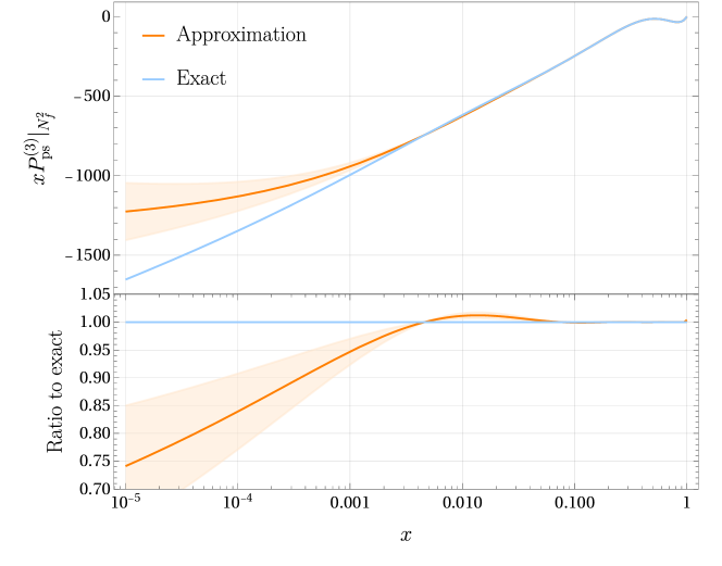
Refer to caption
Figure 2: The $N_{f}^{2}$ contribution to the four-loop pure-singlet splitting function $P^{(3)}_{\text{ps}}$. The exact result derived in this work (blue) and an approximation based on $n\leq 20$ fixed moments and known $x\to 0,1$ terms (orange) are compared. The methodology to determine the approximation and its uncertainty are explained in the text. The bottom panel shows the ratio to the exact result.

In Figure 2 we compare the approximation with our exact result. We observe that the approximation describes the exact result well in the large and moderate-$x$ region, with the deviations being below at most a few percent. However, the small-$x$ region below $x\lesssim 10^{-3}$ is not captured correctly by the approximation. Its uncertainty is underestimated and the best-fit values are systematically above the exact result. This highlights the importance of the divergent terms in the $x\to 0$ limit which were previously unknown and are difficult to constrain from a limited number of Mellin moments.

It is worth noting that our exact results allow one to construct a simple power-logarithmic approximation (involving only the terms of the form $x^{j}\log^{k}(x),~{}(1-x)^{j}\log^{k}(1-x)$) that is precise over the whole $x$ range. For the readers’ convenience, we provide such an approximation below:

$\displaystyle P^{(3)}_{\text{ps}}$ $\displaystyle(x)\big{|}_{N_{f}^{3}}=-\frac{19.6341}{x}-0.197531\log^{4}(x)-3.81893\log^{3}(x)-27.0245\log^{2}(x)$
$\displaystyle-129.255\log(x)-147.059-0.660017x^{5}+0.752343x^{4}-34.9402x^{3}$
$\displaystyle+x^{2}\Big{[}0.252007\log^{4}(x)+0.378676\log^{3}(x)+8.79762\log^{2}(x)+32.774\log(x)$
$\displaystyle+106.766\Big{]}+(1-x)\Big{[}-1.57998\log^{3}(1-x)-7.89567\log^{2}(1-x)$
$\displaystyle-17.8746\log(1-x)\Big{]}+(1-x)^{2}\Big{[}-0.185609\log^{3}(1-x)-1.90667\log^{2}(1-x)$
$\displaystyle-7.06942\log(1-x)\Big{]}+x\Big{[}-0.198775\log^{4}(x)-3.87072\log^{3}(x)-27.8681\log^{2}(x)$
$\displaystyle-110.358\log(x)+94.7747\Big{]}\,,$ (60)
$\displaystyle P^{(3)}_{\text{ps}}$ $\displaystyle(x)\big{|}_{N_{f}^{2}}=\frac{114.438\log(x)}{x}-\frac{356.614}{x}+0.790123\log^{6}(x)+3.79259\log^{5}(x)$
$\displaystyle+77.3663\log^{4}(x)+314.204\log^{3}(x)+1258.40\log^{2}(x)+949.678\log(x)-49.9323$
$\displaystyle+33.627x^{5}-287.064x^{4}+9680.22x^{3}+x^{2}\Big{[}-4.63175\log^{6}(x)-11.7058\log^{5}(x)$
$\displaystyle-393.364\log^{4}(x)-418.965\log^{3}(x)-8435.97\log^{2}(x)+1319.27\log(x)-21652.5\Big{]}$
$\displaystyle+(1-x)^{2}\Big{[}-4.84858\log^{4}(1-x)+8.27339\log^{3}(1-x)-92.6823\log^{2}(1-x)$
$\displaystyle+161.418\log(1-x)\Big{]}+(1-x)\Big{[}3.63945\log^{4}(1-x)+41.3407\log^{3}(1-x)$
$\displaystyle+228.914\log^{2}(1-x)+761.999\log(1-x)\Big{]}+x\Big{[}0.783717\log^{6}(x)+0.335522\log^{5}(x)$
$\displaystyle+1.53492\log^{4}(x)-192.192\log^{3}(x)+358.62\log^{2}(x)-884.842\log(x)+12632.2\Big{]}$
$\displaystyle+0.0000703741\,,$ (61)

where we have set $C_{A}=3,\,C_{F}=4/3$ and truncated the numerical values of the coefficients to 6 digits. This approximation has an accuracy better than $10^{-5}$ over the whole range of $x$. It can be readily included in the programs implementing scale evolution of parton distribution functions.

5 Conclusions and Outlook

In this paper, we derived the renormalization of the quark singlet operator to four-loop order. We observe that it does not require the computation of new renormalization counterterms beyond those that were already obtained for symbolic Mellin-$n$ in Gehrmann:2023ksf .

As a first non-trivial application, we computed the $N_{f}^{2}$ contributions to the four-loop pure-singlet splitting functions. Our workflow to calculate the relevant four-loop OMEs is described in detail and we validate it on an independent rederivation of the four-loop $N_{f}^{2}$ contributions to the non-singlet splitting functions, giving full agreement with Davies:2016jie . We employ our setup to derive the pure-singlet contributions involving two closed fermion loops, for the first time for symbolic $n$. This allowed us to derive the exact results in $x$-space and to perform a comparison with an approximation obtained from the fixed $n\leq 20$ results. We demonstrated that the approximation is adequate for large to moderate values of $x$, but fails to correctly capture the behavior at small values of $x$. It would be interesting to investigate if this has tangible implications for the construction of approximate N3LO parton distributions functions McGowan:2022nag ; Hekhorn:2023gul .

Building on the methodology presented here, the complete computation of all color and flavor structures for the singlet, four-loop splitting functions can be envisaged. Towards this objective, we expect a considerable increase in complexity, in particular for the required integral reductions. Moreover, the computation of the splittings into gluons involves the renormalization of the gluon operator up to four loops and will likely require new counterterms whose Feynman rules remain to be determined.

Acknowledgements.
We would like to thank Giulio Falcioni, Franz Herzog, Sven-Olaf Moch and Andreas Vogt for constructive discussions. We acknowledge the European Research Council (ERC) for funding of this work under the European Union’s Horizon 2020 research and innovation programme grant agreement 101019620 (ERC Advanced Grant TOPUP) and the National Science Foundation (NSF) for support under grant number 2013859.

Appendix A Standard QCD renormalization constant

The strong coupling renormalization constant $Z_{a_{s}}$ can be expressed through the QCD $\beta$ function,

$\displaystyle Z_{a_{s}}=1-\frac{\beta_{0}}{\epsilon}a_{s}+\left(\frac{\beta_{0}^{2}}{\epsilon^{2}}-\frac{\beta_{1}}{2\epsilon}\right)a_{s}^{2}+\left(-\frac{\beta_{0}^{3}}{\epsilon^{3}}+\frac{7\beta_{0}\beta_{1}}{6\epsilon^{2}}-\frac{\beta_{2}}{3\epsilon}\right)a_{s}^{3}+\mathcal{O}(a_{s}^{4}).$ (62)

Up to three loops, the QCD beta function reads Tarasov:1980au

$\displaystyle\beta_{0}$ $\displaystyle=\frac{11C_{A}}{3}-\frac{2N_{f}}{3}\,,$ (63)
$\displaystyle\beta_{1}$ $\displaystyle=-\frac{10C_{A}N_{f}}{3}+\frac{34C_{A}^{2}}{3}-2C_{F}N_{f}\,,$ (64)
$\displaystyle\beta_{2}$ $\displaystyle=-\frac{1415}{54}C_{A}^{2}N_{f}+\frac{79}{54}C_{A}N_{f}^{2}-\frac{205}{18}C_{A}C_{F}N_{f}+\frac{2857C_{A}^{3}}{54}+\frac{11}{9}C_{F}N_{f}^{2}+C_{F}^{2}N_{f}\,.$ (65)

The gluon field renormalization constant

$\displaystyle Z_{g}=\sum_{l=0}^{\infty}Z_{g}^{(l)}a_{s}^{l}$ (66)

is required to three-loop order Tarasov:1980au ; Larin:1993tp for this work. The relevant expansion coefficients read

$\displaystyle Z_{g}^{(0)}=$ $\displaystyle 1\,,$ (67)
$\displaystyle Z_{g}^{(1)}=$ $\displaystyle\frac{1}{\epsilon}\bigg{[}\left(\frac{13}{6}-\frac{\xi}{2}\right)C_{A}-\frac{2N_{f}}{3}\bigg{]}\,,$ (68)
$\displaystyle Z_{g}^{(2)}=$ $\displaystyle\frac{1}{\epsilon}\bigg{[}-\frac{5C_{A}N_{f}}{4}+\left(-\frac{\xi^{2}}{8}-\frac{11\xi}{16}+\frac{59}{16}\right)C_{A}^{2}-C_{F}N_{f}\bigg{]}$
$\displaystyle+\frac{1}{\epsilon^{2}}\bigg{[}\left(\frac{\xi}{3}+\frac{1}{2}\right)C_{A}N_{f}+\left(\frac{\xi^{2}}{4}-\frac{17\xi}{24}-\frac{13}{8}\right)C_{A}^{2}\bigg{]}\,,$ (69)
$\displaystyle Z_{g}^{(3)}=$ $\displaystyle\frac{1}{\epsilon^{2}}\bigg{[}C_{F}\bigg{\{}\left(\frac{\xi}{2}+\frac{31}{18}\right)C_{A}N_{f}-\frac{2N_{f}^{2}}{9}\bigg{\}}+\left(\frac{\xi^{2}}{12}+\frac{19\xi}{24}+\frac{481}{108}\right)C_{A}^{2}N_{f}-\frac{25}{54}C_{A}N_{f}^{2}$
$\displaystyle+\left(\frac{7\xi^{3}}{48}+\frac{13\xi^{2}}{24}-\frac{143\xi}{96}-\frac{7957}{864}\right)C_{A}^{3}\bigg{]}+\frac{1}{\epsilon}\bigg{[}C_{F}\bigg{\{}\left(-4\zeta_{3}-\frac{5}{108}\right)C_{A}N_{f}+\frac{11N_{f}^{2}}{27}\bigg{\}}$
$\displaystyle+C_{A}^{2}N_{f}\left(\frac{\xi}{3}+3\zeta_{3}-\frac{911}{108}\right)+\frac{19}{27}C_{A}N_{f}^{2}+C_{A}^{3}\bigg{\{}-\frac{7\xi^{3}}{96}+\xi^{2}\left(-\frac{\zeta_{3}}{16}-\frac{11}{32}\right)$
$\displaystyle+\xi\left(-\frac{\zeta_{3}}{4}-\frac{167}{96}\right)-\frac{3\zeta_{3}}{16}+\frac{9965}{864}\bigg{\}}+\frac{1}{3}C_{F}^{2}N_{f}\bigg{]}+\frac{1}{\epsilon^{3}}\bigg{[}\left(-\frac{\xi^{2}}{6}-\frac{5\xi}{12}-\frac{11}{9}\right)C_{A}^{2}N_{f}$
$\displaystyle+\frac{1}{9}C_{A}N_{f}^{2}+\left(-\frac{\xi^{3}}{8}+\frac{\xi^{2}}{6}+\frac{47\xi}{48}+\frac{403}{144}\right)C_{A}^{3}\bigg{]}\,.$ (70)

The quark field renormalization constant

$\displaystyle Z_{q}=\sum_{l=0}^{\infty}Z_{q}^{(l)}a_{s}^{l}$ (71)

is required to four-loop order Chetyrkin:1999pq ; Chetyrkin:2004mf . The relevant expansion coefficients read

$\displaystyle Z_{q}^{(0)}=$ $\displaystyle 1\,,$ (72)
$\displaystyle Z_{q}^{(1)}=$ $\displaystyle-C_{F}\frac{\xi}{\epsilon}\,,$ (73)
$\displaystyle{Z_{q}^{(2)}}=$ $\displaystyle\frac{C_{F}}{\epsilon}\bigg{[}\left(-\frac{\xi^{2}}{8}-\xi-\frac{25}{8}\right)C_{A}+\frac{3C_{F}}{4}+\frac{N_{f}}{2}\bigg{]}+\frac{C_{F}}{\epsilon^{2}}\bigg{[}\left(\frac{\xi^{2}}{4}+\frac{3\xi}{4}\right)C_{A}+\frac{\xi^{2}C_{F}}{2}\bigg{]}\,,$ (74)
$\displaystyle{Z_{q}^{(3)}}=$ $\displaystyle\frac{C_{F}}{\epsilon^{3}}\bigg{[}C_{A}\left(\Big{(}-\frac{\xi^{3}}{4}-\frac{3\xi^{2}}{4}\Big{)}C_{F}+\frac{\xi N_{f}}{6}\right)+\left(-\frac{\xi^{3}}{12}-\frac{3\xi^{2}}{8}-\frac{31\xi}{24}\right)C_{A}^{2}-\frac{1}{6}\xi^{3}C_{F}^{2}\bigg{]}$
$\displaystyle+\frac{C_{F}}{\epsilon^{2}}\bigg{[}C_{A}\left(\left(\frac{\xi^{3}}{8}+\xi^{2}+\frac{25\xi}{8}-\frac{11}{6}\right)C_{F}+\left(-\frac{\xi}{2}-\frac{47}{18}\right)N_{f}\right)$
$\displaystyle+\left(\frac{\xi^{3}}{8}+\frac{3\xi^{2}}{4}+\frac{73\xi}{24}+\frac{275}{36}\right)C_{A}^{2}+\left(\frac{1}{3}-\frac{\xi}{2}\right)C_{F}N_{f}-\frac{3\xi C_{F}^{2}}{4}+\frac{2N_{f}^{2}}{9}\bigg{]}$
$\displaystyle+\frac{C_{F}}{\epsilon}\bigg{[}C_{A}\left(\Big{(}\frac{143}{12}-4\zeta_{3}\Big{)}C_{F}+\Big{(}\frac{17\xi}{24}+\frac{287}{54}\Big{)}N_{f}\right)-\frac{C_{F}N_{f}}{2}-\frac{C_{F}^{2}}{2}-\frac{5N_{f}^{2}}{27}$
$\displaystyle+C_{A}^{2}\bigg{\{}-\frac{5\xi^{3}}{48}+\xi^{2}\left(-\frac{\zeta_{3}}{8}-\frac{13}{32}\right)+\xi\left(-\frac{\zeta_{3}}{4}-\frac{263}{96}\right)+\frac{23\zeta_{3}}{8}-\frac{9155}{432}\bigg{\}}\bigg{]}\,,$ (75)
$\displaystyle Z_{q}^{(4)}\big{|}_{N_{f}^{3}}=$ $\displaystyle\frac{C_{F}}{9\epsilon^{3}}-\frac{5C_{F}}{54\epsilon^{2}}-\frac{35C_{F}}{324\epsilon}\,,$ (76)
$\displaystyle Z_{q}^{(4)}\big{|}_{N_{f}^{2}}=$ $\displaystyle\frac{\xi C_{F}C_{A}}{18\epsilon^{4}}+\frac{C_{F}}{\epsilon^{3}}\bigg{[}\left(-\frac{\xi}{6}-\frac{23}{12}\right)C_{A}+\left(\frac{1}{6}-\frac{2\xi}{9}\right)C_{F}\bigg{]}$
$\displaystyle+\frac{C_{F}}{\epsilon^{2}}\bigg{[}\left(\frac{2\xi}{27}+4\right)C_{A}+\left(\frac{5\xi}{27}+\frac{3}{8}\right)C_{F}\bigg{]}$
$\displaystyle+\frac{C_{F}}{{\epsilon}}\bigg{[}C_{A}\left(\left(\frac{269}{972}-\frac{\zeta_{3}}{3}\right)\xi-2\zeta_{3}-\frac{293}{144}\right)+\left(2\zeta_{3}-\frac{19}{9}\right)C_{F}\bigg{]}.$ (77)

We note that at four loops, only the $N_{f}^{3}$ and $N_{f}^{2}$ terms contribute to the calculation presented in this paper.

References