Time-fractional Caputo derivative versus other integro-differential operators in generalized Fokker-Planck and generalized Langevin equations

Abstract

Fractional diffusion and Fokker-Planck equations are widely used tools to describe anomalous diffusion in a large variety of complex systems. The equivalent formulations in terms of Caputo or Riemann-Liouville fractional derivatives can be derived as continuum limits of continuous time random walks and are associated with the Mittag-Leffler relaxation of Fourier modes, interpolating between a short-time stretched exponential and a long-time inverse power-law scaling. More recently, a number of other integro-differential operators have been proposed, including the Caputo-Fabrizio and Atangana-Baleanu forms. Moreover, the conformable derivative has been introduced. We here study the dynamics of the associated generalized Fokker-Planck equations from the perspective of the moments, the time averaged mean squared displacements, and the autocovariance functions. We also study generalized Langevin equations based on these generalized operators. The differences between the Fokker-Planck and Langevin equations with different integro-differential operators are discussed and compared with the dynamic behavior of established models of scaled Brownian motion and fractional Brownian motion. We demonstrate that the integro-differential operators with exponential and Mittag-Leffler kernels are not suitable to be introduced to Fokker-Planck and Langevin equations for the physically relevant diffusion scenarios discussed in our paper. The conformable and Caputo Langevin equations are unveiled to share similar properties with scaled and fractional Brownian motion, respectively.

I Introduction

Power-laws and fractional derivatives have a long tradition in the sciences. Thus, Buelffinger modified Hooke’s law to a general power exponent in 1729 buel ; reiner . Weber is credited for having (indirectly) discovered viscoelasticity, following his report of a non-elastic aftereffect in stretched silk threads in 1835 marko , an effect that initiated the development of generalized rheological models tschoegl . An explicit time dependence deviating from the exponential law was proposed by Kohlrausch in 1847 in the form of a stretched exponential, introducing a fractional power-law into an exponential function marko . Power-law time dependencies in relaxation phenomena were reported by Nutting in 1921 nutting . To grasp such a behavior in a compact dynamic equation, Scott Blair then formulated a relaxation equation with a fractional derivative scott . Fractional rheological models have since been used widely to describe the viscoelastic or glassy behavior in complex systems wg ; jcp95 ; helmut ; hilfer ; mainardibook . Fractional relaxation processes are also relevant in biological contexts wg1 ; hilfer2000applications .

Fractional derivatives have also found widespread use in the context of anomalous diffusion, typically defined in terms of the power-law form report ; resto ; pccp ; hoefling ; evangelista2018fractional

$$\langle x^{2}(t)\rangle\simeq K_{\alpha}t^{\alpha}$$ (1)

of the mean squared displacement (MSD). Here $K_{\alpha}$ of physical dimension $\mathrm{length}^{2}/\mathrm{time}^{\alpha}$ is the generalized diffusion coefficient and the value of the anomalous diffusion exponent $\alpha$ distinguishes subdiffusion ($0<\alpha<1$) from superdiffusion ($\alpha>1$), including the special cases of normal diffusion ($\alpha=1$) and ballistic, wave-like motion ($\alpha=2$). A breakthrough in describing anomalous diffusion came with the work of Schneider and Wyss schneider , who started from the integral version of the diffusion equation

$$P(x,t)-P_{0}(x)=K_{1}\int_{0}^{t}\frac{\partial^{2}}{\partial x^{2}}P(x,t^{\prime})dt^{\prime}$$ (2)

for the probability density function $P(x,t)$ to find the test particle at position $x$ at time $t$, given the initial condition $P_{0}(x)$ at $t=0$. They then replaced the integral by a Riemann-Liouville (RL) fractional integral operator defined for a suitable function $f(t)$ as oldham ; miller

$${}_{0}D_{t}^{-\alpha}f(t)=\frac{1}{\Gamma(\alpha)}\int_{0}^{t}\frac{f(t^{\prime})}{(t-t^{\prime})^{1-\alpha}}dt^{\prime},$$ (3)

which is a direct generalization of the Cauchy multiple integral. After differentiation by time once one obtains the equivalent fractional diffusion equation (FDE) in RL-form report

$$\frac{\partial}{\partial t}P(x,t)=K_{\alpha}\,{}_{0}D_{t}^{1-\alpha}\frac{\partial^{2}}{\partial x^{2}}P(x,t),$$ (4)

where ${}_{0}D_{t}^{1-\alpha}=(d/dt)\,_{0}D_{t}^{-\alpha}$ is the RL fractional differential operator oldham ; miller . The solution of the FDE (4) can be obtained in terms of Fox $H$-functions schneider ; report ; mathai . The asymptotic behavior of the PDF $P(x,t)$ encoded in the FDE (4) has a stretched Gaussian shape schneider ; klazu ; report . FDEs of the above form can be derived as the continuum limit of continuous time random walks (CTRWs) with scale-free waiting time densities $\psi(t)\simeq t^{-1-\alpha}$ with $0<\alpha<1$ and jump length densities with finite variance compte ; hilfer1995fractional ; mebakla1 ; bakai2001 ; klazu ; report ; thiel2014scaled . By single-particle tracking method waiting time densities with power-law forms were revealed, i.a., in protein motion in membranes weigel , colloidal tracer motion in actin networks weitz ; yael , orfor tracers in non-laminar flows swinney . Power-law waiting time densities were also identified in dynamic maps geisel or simulations of drug molecules diffusing in silica slits amanda . When an external potential influences the particle motion, the FDE (4) can be generalized to the fractional Fokker-Planck equation mebakla ; bakai2001 ; mebakla1 ; klazu ; report ; magdziarz2007fractional ; stanislavsky2008diffusion ; gorska2012operator . For transport in groundwater and other applications advection terms as well as mobile-immobile scenarios are considered in generalized versions of FDEs schumer2009fractional ; schumer2003fractal ; timo ; dentz2004time ; meerschaert2008tempered ; harvey ; brian ; brian1 ; berkowitz2006modeling . In the context of FDEs and fractional Fokker-Planck equations of RL-type the relaxation of modes follows the Mittag-Leffler pattern (see below) that interpolates between an initial stretched exponential and a long-time inverse power-law wg ; report .

Apart from the mentioned RL fractional derivatives, there exist a wide variety of other types of fractional derivatives samko1993fractional ; podlubny1999fractional ; kilbas2006theory ; hilferdesi , many of which are being used in engineering and science applications. Possibly the most widely used apart from the RL definition is the Caputo fractional derivative caputo1966linear ; caputo1967linear . We note that both definitions are in fact equivalent as long as the initial values are properly taken into account. Thus, when we solve the FDE (4) for a specific initial value problem the Caputo version of the FDE studied below leads to the same result. Caputo fractional derivatives are used, i.a., to model non-Darcian flow zhou2018fractional , permeability models for rocks yang2019fractional , contaminant transport benson2013fractional , or viscoelastic diffusion caputo2004diffusion ; caputo1999diffusion . Apart from the Caputo or RL derivative based on a power-law integral kernel with a (weak) singularity, in the last decade some new non-singular integro-differential operators have been proposed. One option is the Caputo-Fabrizio (CF) integro-differential operator with exponential kernel caputo2015new . The CF operator was employed in a number of areas, for instance, fluid flow sheikh2018modern , virus models khan2019modeling ; baleanu2020fractional , and a human liver model baleanu2020new . Alternatively, the Atangana-Baleanu (AB) integro-differential operator based on the Mittag-Leffler function for the memory kernel atangana2016new aims to describe the full memory effect in systems since the Mittag-Leffler function combines a stretched exponential shape and a power-law decay at short and long times, respectively. The AB operator is used in FDEs sene2019analysis , Cauchy and source problems for advection-diffusion avci2019cauchy , optimal control ammi2019optimal , and disease models baleanu2020modelling . Comparisons between the AB and CF integro-differential operators are investigated in relaxation and diffusion models sun2017relaxation , reaction-diffusion models shaikh2019analysis , cancer models gomez2017chaos , heat transfer analysis siddique2021heat , and for the Casson fluid ali2019effects .

Apart from the non-local integro-differential operators mentioned above, a local derivative, the so-called conformable derivative, has been introduced A7 ; anderson2015newly ; atangana2015new ; fleitas2021note and studied from a physical point of view zhao2017general . Applications of the conformable derivative formulation have been discussed for anomalous diffusion 18 , advection-diffusion Y ; 2020Analytical , non-Darcian flow yang2018conformable , and other differential equations ccenesiz2017new ; korpinar2019new ; cevikelsolitary ; akbulut2018auxiliary ; hyder2020exact . A similar variant is the Hausdorff derivative proposed earlier by Chen chen2006time . This derivative is also employed in diffusion scenarios chen2010anomalous ; chen2017new ; liang2019distributed ; liang2019time ; liang2019hausdorff1 , anomalous diffusion in magnetic resonance imaging liang2016fractal , viscoelastic modeling cai2016characterizing , or the Richards’ equation sun2013fractal . It was shown that the conformable derivative is in fact proportional to the Hausdorff derivative weberszpil2016variational ; rosa2018dual . Further discussions of these derivatives can be found in diethelm2020fractional ; giusti2018comment ; anderson2018nature .

We here scrutinize the recently integro-differential operators proposed in the framework of FDEs and generalized Fokker-Planck equations as well as their applications in generalizations of the stochastic Langevin equations. Fourier and Laplace transforms are used to obtain analytical solutions for the PDFs and the moments to study the dynamics encoded in these dynamic equations. In particular we unveil the connections between FDEs and fractional Langevin equations with other well-known stochastic processes, particularly with scaled Brownian motion (SBM, based on a Langevin equation with deterministic power-law time dependence of the diffusion coefficient) and fractional Brownian motion (FBM, based on a Langevin equation driven by zero-mean Gaussian noise with long-range, power-law correlations). Our discussion is based on experimentally measurable quantities. These include the first and second moments, the MSD, and the PDF. Moments can be directly inferred from measured time series as either ensemble or time averages barkai2012single . PDFs can also be reconstructed in many contemporary studies and used, inter alia, to check for non-Gaussianity features ng .

The paper is structured as follows. In Sec. II we introduce and briefly discuss different integro-differential operators and recall the generalized Fokker-Planck and Langevin equations in describing stochastic processes in complex systems. In Sec. III we discuss the results of local and non-singular integro-differential operators in Fokker-Planck equations for the force-free case and for a constant drift. Specifically we discuss the extent to which the CF and AB integro-differential operators can provide physically meaningful descriptions in the anomalous diffusion context. The results of the conformable and Caputo diffusion equations (with drift) and SBM (with drift) are compared. In Sec. IV we focus on generalized Langevin equations for SBM and FBM, as well as Langevin equations with the four integro-differential operators introduced in Sec. II. Specifically, we again discuss the physical implications of the CF and AB integro-differential operators in this context. The related moments, time averaged MSD (TAMSD), and autocovariance function (ACVF) are considered to assess different Langevin equations. In Sec. V, we summarize and discuss our results. We also present two tables with the main results for the generalized Fokker-Planck and Langevin equations discussed in the paper.

II Integro-differential operators, generalized Fokker-Planck and Langevin equations

In this Section, we provide a brief introduction to four definitions of integro-differential operators that are frequently employed in theoretical modeling and engineering, the Caputo derivative (note our remarks to the extent these are equivalent to the RL-derivative) and conformable derivative, as well as the two recently proposed CF and AB integro-differential operators. We then introduce them to generalized formulations of the Fokker-Planck and Langevin equations.

II.1 Integro-differential operators

The Caputo derivative of order $\alpha\in(0,1]$ for a suitable function $f(t)$ is defined in terms of a power-law kernel caputo1966linear ; caputo1967linear ,

$$^{C}_{0}D^{\alpha}_{t}f(t)=\frac{1}{\Gamma(1-\alpha)}\int_{0}^{t}\frac{f^{\prime}(t^{\prime})}{(t-t^{\prime})^{\alpha}}dt^{\prime},$$ (5)

where $f^{\prime}(t)=df(t)/dt$. The Caputo derivative thus has a (weak) singularity at $t^{\prime}=t$. The special feature introduced by Caputo in his derivative is the fact that the derivative on the function $f(t)$, $f^{\prime}(t)=df(t)/dt$, is contained inside the integral. This contrasts the definition of the RL fractional derivative, in which the differentiation is taken after the fractional integration oldham ; report . In the Caputo formulation, e.g., when using Laplace transform methods to derive the solution, the initial conditions thus enter in the traditional way. For $0<\alpha<1$, e.g., the initial value of $f(t)$ at $t=0$ is needed. This contrasts the RL derivative, for which fractional-order initial conditions enter oldham . However, this complication for the RL derivative can be circumvented in the Schneider and Wyss integral formulation presented above schneider ; wg ; wg1 ; report ; resto ; mebakla ; bakai2001 ; mebakla1 . In the solution of time-fractional equations with initial condition given at $t=0$, the Laplace transform

$$\mathscr{L}\{f(t)\}(s)\equiv\tilde{f}(s)=\int_{0}^{\infty}f(t)\exp(-st)dt$$ (6)

is of central importance. For the fractional RL-Integral, the Laplace transform reads $\mathscr{L}\{f(t)\}=s^{-\alpha}\tilde{f}(s)$, and for the Caputo-fractional operator we have

$$\mathscr{L}\left\{\,{}^{C}_{0}D^{\alpha}_{t}f(t)\right\}=s^{\alpha}\tilde{f}(s)-s^{\alpha-1}f(0).$$ (7)

Recently, two new definitions of integro-differential operators with non-singular kernel were proposed. One is the Caputo-Fabrizio (CF) integro-differential operator of order $\alpha\in(0,1]$ defined with an exponential kernel caputo2015new ,

$$^{CF}_{0}D^{\alpha}_{t}f(t)=\frac{M(\alpha)}{(1-\alpha)\tau^{\alpha}}\int_{0}^{t}f^{\prime}(t^{\prime})\exp\left(\frac{-\alpha(t-t^{\prime})}{(1-\alpha)\tau}\right)dt^{\prime},$$ (8)

where the factor $M(\alpha)$ introduced in caputo2015new is chosen such that $M(0)=M(1)=1$. Note that we introduced the time scale $\tau$ in order to get dimensions correct. The choice $\tau^{\alpha}$ in the factor in front of the exponential allows us to take the limits $\alpha=0$ (where we get $f(t)-f(0)$) and $\alpha=1$ (the normal differential) consistently. The Laplace transform of the CF-operator reads

$$\mathscr{L}\left\{\,{}^{CF}_{0}D^{\alpha}_{t}f(t)\right\}=\frac{s\tilde{f}(s)-f(0)}{(1-\alpha)\tau^{\alpha}s+\alpha\tau^{\alpha-1}}.$$ (9)

The other variant for a generalized fractional derivative is given by the Atangana-Baleanu (AB) integro-differential operator with Mittag-Leffler kernel atangana2016new ,

$$^{AB}_{0}D^{\alpha}_{t}f(t)=\frac{B(\alpha)}{(1-\alpha)\tau^{\alpha}}\int_{0}^{t}f^{\prime}(t^{\prime})E_{\alpha}\left(-\alpha\frac{(t-t^{\prime})^{\alpha}}{(1-\alpha)\tau^{\alpha}}\right)dt^{\prime},$$ (10)

where $E_{\alpha}(-z)=\sum_{k=0}^{\infty}(-z)^{k}/\Gamma(1+\alpha k)$ is the one-parameter Mittag-Leffler function with expansion around infinity $E_{\alpha}(-z)\sim-\sum_{k=1}^{\infty}(-z)^{-k}/\Gamma(1-\alpha k)$ erdelyi . In particular, when $\alpha=1$, $E_{1}(z)=e^{z}$. Note that we again introduced the time scale $\tau$ for dimensional consistency. Moreover, we note that here $B(\alpha)$ is a normalization function satisfying $B(0)=B(1)=1$ and has the same properties as in the CF operator. To simplify our notation in the following, we set $M(\alpha)=B(\alpha)=1$ caputo2015new ; atangana2016new . The Laplace transform of the AB-operator has the form

$$\mathscr{L}\left\{\,{}^{AB}_{0}D^{\alpha}_{t}f(t)\right\}=\frac{s^{\alpha}\tilde{f}(t)-s^{\alpha-1}f(0)}{(1-\alpha)\tau^{\alpha}s^{\alpha}+\alpha}.$$ (11)

All these definitions, Caputo, CF, and AB integro-differential operators correspond to convolutions of the derivative $f^{\prime}(t)$ with different choices for the kernels, i.e., power-law, exponential, and Mittag-Leffler functions, respectively. In contrast, there also exists a local definition of a generalized derivative, namely, the conformable derivative of order $\alpha\in(0,1]$, defined via khalil2014new

$$T_{\alpha}f(t)=\lim\limits_{\bar{\tau}\to 0}\frac{f(t+\bar{\tau}^{\alpha}t^{1-\alpha})-f(t)}{\bar{\tau}^{\alpha}}.$$ (12)

Here we used the small variable $\bar{\tau}$ with dimension of time to housekeep physical dimensions. If the conformable derivative of $f$ of order $\alpha$ exists in some interval $(0,a)$, $a>0$, and $\lim\limits_{t\to 0^{+}}T_{\alpha}f(t)$ exists, then we define $T_{\alpha}f(0)=\lim\limits_{t\to 0^{+}}T_{\alpha}f(t)$. The conformable Laplace transform of $f(t)$ is defined by A7

$$\mathscr{L}_{\alpha}\left\{f(t)\right\}(s)\equiv\tilde{f}_{\alpha}(s)=\int_{0}^{\infty}f(t)t^{\alpha-1}\exp\left(-s\frac{t^{\alpha}}{\alpha}\right)dt,$$ (13)

generalizing the standard Laplace transform (6). The relationship between the conformable Laplace transform and the ordinary Laplace transform is $\mathscr{L}_{\alpha}\{f(t)\}(s)=\mathscr{L}\{f(\alpha t)^{1/\alpha)}\}(s)$. The conformable Laplace transform of the conformable derivative is

$$\mathscr{L}_{\alpha}\{T_{\alpha}f(t)\}(s)=s\tilde{f}_{\alpha}(s)-f(0).$$ (14)

The Hausdorff derivative (fractal derivative) of a suitable function $f(t)$ with respect to $t^{\alpha}$ chen2006time is defined as

$$\frac{df(t)}{dt^{\alpha}}=\lim_{t^{\prime}\rightarrow t}\frac{f(t)-f(t^{\prime})}{t^{\alpha}-(t^{\prime})^{\alpha}}.$$ (15)

From this definition we see that the Hausdorff derivative is also local in nature. The connection between the Hausdorff derivative and the conformable derivative is given by weberszpil2016variational ; rosa2018dual ,

$$\alpha\frac{df(t)}{dt^{\alpha}}=t^{1-\alpha}\frac{df(t)}{dt}=T_{\alpha}f(t).$$ (16)

II.2 Generalized Fokker-Planck equations

We now use these operators to generalize the Fokker-Planck equation risken

$$\frac{\partial}{\partial t}P(x,t)=\left(K_{1}\frac{\partial^{2}}{\partial x^{2}}-\frac{\partial}{\partial x}\frac{F(x)}{m\eta}\right)P(x,t)$$ (17)

in the presence of a general external force field $F(x)$. Here $m$ is the particle mass and $\eta$ the friction coefficient risken . For the force, we obtain solutions for vanishing or constant external force $F_{0}$. In the latter case, we then use the drift velocity $v=F_{0}/(m\eta)$. In the generalization based on the RL derivative the fractional Fokker-Planck equation was analyzed for different linear and non-linear force fields bakai2001 ; mebakla ; report ; resto .

We here introduce the four generalized differential operators above and analyze the generalized diffusion equation (GDE) or generalized diffusion equation with drift (drift-GDE)

$$\frac{\partial^{\alpha}}{\partial t^{\alpha}}P(x,t)=\left(K_{\alpha}\frac{\partial^{2}}{\partial x^{2}}-v_{\alpha}\frac{\partial}{\partial x}\right)P(x,t)$$ (18)

with initial condition $P(x,0)=\delta(x)$, for $v_{\alpha}=0$ and $v_{\alpha}\neq 0$ and "natural" boundary conditions $P(|x|\to\infty,t)=0$. These standard initial and boundary conditions will be applied throughout this work. Note that we introduced the $\alpha$-dependent velocity $v_{\alpha}$ for dimensionality housekeeping purposes. This can be achieved by setting $v_{\alpha}=v\tau^{1-\alpha}$, where $\tau$ is a time scale, such that $v_{\alpha}$ has dimension $\mathrm{length}/\mathrm{time}^{\alpha}$. We seek solutions of Eq. (18) on the infinite line $-\infty<x<\infty$, and the notation $\partial^{\alpha}/\partial t^{\alpha}$ represents our four operators.

For our analysis, we also need to introduce SBM lim2002self ; jeon2014scaled , whose diffusion coefficient is explicitly time-dependent and evolves as power-law $\mathscr{K}_{\alpha}(t)=\alpha K_{\alpha}t^{\alpha-1}$ with $\alpha>0$. SBM is a Gaussian self-similar Markovian process with independent but non-stationary increments. It finds applications in turbulence batchelor1952 , stochastic hydrology talkner2011 , finance bassler2007 , granular gases bodrova2015 , and magnetic resonance imaging novikov2014 , to name a few. The Fokker-Planck equation for SBM in an external force field is given by jeon2014scaled

$$\frac{\partial}{\partial t}P(x,t)=\left(\mathscr{K}_{\alpha}(t)\frac{\partial^{2}}{\partial x^{2}}-\frac{\partial}{\partial x}\frac{F(x)}{m\eta}\right)P(x,t).$$ (19)

II.3 Generalized Langevin equations

Fokker-Planck equations are deterministic equations for the PDF $P(x,t)$. A stochastic description of the position of a test particle in the presence of a fluctuating force is the Langevin equation coffey , the alternative standard description of diffusive processes vankampen . The (overdamped) Langevin equation corresponding to the Fokker-Planck equation (17) with $P_{0}(x)=\delta(x)$ reads

$$\frac{d}{dt}x(t)=\frac{F(x)}{m\eta}+\sqrt{2K_{1}}\xi(t),$$ (20)

with the initial position $x(0)=0$. Here $\xi(t)$ is zero-mean white Gaussian noise with ACVF $\langle\xi(t)\xi(t^{\prime})\rangle=\delta(t-t^{\prime})$. Then, the generalized Langevin equation for the thermalized system in the overdampeld approximation reads zwanzig2001

$$\int_{0}^{t}\gamma\left(t-t^{\prime}\right)\frac{\mathrm{d}x\left(t^{\prime}\right)}{\mathrm{d}t^{\prime}}\mathrm{d}t^{\prime}=\frac{F(x)}{m\eta}+\frac{\zeta(t)}{m\eta},$$ (21)

where the noise autocorrelation function is coupled to the frictional kernel by the Kubo-Zwanzig fluctuation-dissipation theorem (FDT) kubo1966 $\left\langle\zeta(t_{1})\zeta(t_{2})\right\rangle=k_{B}Tm\eta\gamma\left(t_{1}-t_{2}\right)$, where $k_{B}$ is the Boltzmann constant and $T$ is the absolute temperature of the environment. The noise $\zeta(t)$ obeying the FDT is called internal. Generalized Langevin equations with FDT and different kernels, e.g., of exponential and Mittag-Leffler shapes have been extensively studied before vinales2007 ; figueiredo2009 ; liemert2017 ; fa2006 ; porra1996 .

In what follows we generalize the Langevin equation (20) via the four operators in Eqs. (5), (8), (10), and (12), in presence of a constant force, with the unifying notation

$$\frac{d^{\alpha}}{dt^{\alpha}}x(t)=v_{\alpha}+\sqrt{2K_{\alpha}}\xi(t),$$ (22)

We note that FBM and the generalized Langevin equations we consider here do not fulfill the generalized fluctuation-dissipation theorem and thus do not describe equilibrium systems. Instead, the noise is considered to be external klimo . This is appropriate for active systems, in which energy is dissipated, e.g., living biological cells.

We will compare the resulting dynamics with that encoded by SBM, whose Langevin equation is given by lim2002self ; jeon2014scaled

$$\frac{d}{dt}x(t)=\frac{F(x)}{m\eta}+\sqrt{2\mathscr{K}_{\alpha}(t)}\xi(t),$$ (23)

which is equivalent to the deterministic equation (19). The noise $\xi(t)$ has the same properties as for the standard Langevin equation (20), i.e., it is zero-mean white Gaussian noise. In the following we will consider the cases of zero and constant force.

As we will see, it will also be of interest to compare our results to the dynamics of FBM mandelbrot1968fractional , which is stationary in increments and nearly ergodic deng2009ergodic ; pre12 ; lene1 . As a generalization of Brownian motion, FBM is an effective stochastic process to model anomalous diffusion barkai2012single . Its Langevin equation reads mandelbrot1968fractional ; pccp

$$\frac{d}{dt}x(t)=\frac{F(x)}{m\eta}+\sqrt{2K_{\alpha}}\xi_{\alpha}(t),$$ (24)

where $\xi_{\alpha}(t)$ is zero-mean fractional Gaussian noise with the long range, power-law ACVF $\langle\xi_{\alpha}(t_{1})\xi_{\alpha}(t_{2})\rangle\sim\alpha(\alpha-1)|t_{1}-t_{2}|^{\alpha-2}$ when $|t_{1}-t_{2}|\gg 1$. FBM is defined for the range $0<\alpha<2$ of the anomalous diffusion exponent, instead of which the Hurst exponent $H=\alpha/2$ is often used. From the noise ACVF we can see that the noise correlations are positive (persistent) when the motion is superdiffusive, while they are negative (antipersistent) in the subdiffusive case.

We will characterize the dynamics of the processes we consider the moments, the time-averaged MSD (TAMSD) barkai2012single ; pccp , and the displacement ACVF of the process. The TAMSD is important in the analysis of single particle trajectories measured in modern tracking experiments; it is defined via

$$\overline{\delta^{2}(\Delta)}=\frac{1}{T-\Delta}\int_{0}^{T-\Delta}\Big{(}x(t+\Delta)-x(t)\Big{)}^{2}dt,$$ (25)

where $T$ is the length of the time series (measurement time) and $\Delta$ is called the lag time. The mean TAMSD is obtained from averaging over a number $N$ of individual traces $\overline{\delta_{i}^{2}(\Delta)}$,

$$\left<\overline{\delta^{2}(\Delta)}\right>=\frac{1}{N}\sum_{i=1}^{N}\overline{\delta_{i}^{2}(\Delta)}.$$ (26)

In the Birkhoff-Boltzmann sense, a system is considered ergodic when ensemble and time averages are equivalent in the limit of long measurement times. We here consider a stochastic process non-ergodic when the ensemble-averaged MSD and the TAMSD are disparate in the limit of long observation times, $\lim\limits_{T\rightarrow\infty}\overline{\delta^{2}(\Delta)}\neq\langle x^{2}(\Delta)\rangle$. The displacement ACVF is defined as

$$C_{\Delta}(t)=C_{\Delta}(t)=\frac{\langle[x(t+\Delta)-x(t)][x(\Delta)-x(0)]\rangle}{\Delta^{2}}.$$ (27)

III Generalized Fokker-Planck equations

III.1 Generalized Fokker-Planck equations in the force-free case

We now first assess the dynamics encoded in the generalized Fokker-Planck equation (18) in the absence of an external force.

III.1.1 Caputo and non-singular differential operators

When $F(x)=0$, the generalized Fokker-Planck equation (18) reduces to the GDE

$$\frac{\partial^{\alpha}}{\partial t^{\alpha}}P(x,t)=K_{\alpha}\frac{\partial^{2}}{\partial x^{2}}P(x,t),$$ (28)

with $0<\alpha\leq 1$ which we will solve on the interval $-\infty<x<\infty$ for the initial condition $P(x,0)=\delta(x)$. Here the operator $\partial^{\alpha}/\partial t^{\alpha}$ represents the Caputo, CF, and AB integro-differential operators, Eqs. (5), (8), and (10).

Applying the Laplace and Fourier transforms to the GDE (28), we find

$$\hat{\tilde{P}}_{C}(k,s) = \frac{s^{\alpha-1}}{s^{\alpha}+K_{\alpha}k^{2}},$$ (29)

$$\hat{\tilde{P}}_{CF}(k,s) = \frac{1}{s+K_{\alpha}[\alpha\tau^{\alpha-1}+s(1-\alpha)\tau^{\alpha}]k^{2}},$$ (30)

$$\hat{\tilde{P}}_{AB}(k,s) = \frac{s^{\alpha-1}}{s^{\alpha}+K_{\alpha}[\alpha+s^{\alpha}(1-\alpha)\tau^{\alpha}]k^{2}}.$$ (31)

After inverse Fourier transform we obtain the PDFs in Laplace space,

$$\tilde{P}(x,s)=\frac{1}{2s}\phi(s)\exp\left(-\phi(s)|x|\right),$$ (32)

where we define

$$\phi_{C}(s) = \sqrt{\frac{s^{\alpha}}{K_{\alpha}}},$$ (33)

$$\phi_{CF}(s) = \sqrt{\frac{s}{(1-\alpha)\tau^{\alpha}K_{\alpha}s+\alpha\tau^{\alpha-1}K_{\alpha}}},$$ (34)

$$\phi_{AB}(s) = \sqrt{\frac{s^{\alpha}}{(1-\alpha)\tau^{\alpha}K_{\alpha}s^{\alpha}+\alpha K_{\alpha}}},$$ (35)

for the three operators, respectively.

We first recall the PDF of the Caputo diffusion equation based on the Caputo operator (5) in $(x,t)$-space,

$$P_{C}(x,t)=\frac{1}{2\sqrt{K_{\alpha}t^{\alpha}}}M_{\alpha/2}\left(\frac{|x|}{\sqrt{K_{\alpha}t^{\alpha}}}\right),$$ (36)

where $M_{\nu}$ denotes the Mainardi function mainardi2003wright ; gorenflo2007analytical , also called $M$ function (of the Wright type), of order $\nu$. Using the asymptotic representation of $M_{\alpha/2}$ the PDF $P_{C}(x,t)$ can be shown to have a stretched Gaussian shape mainardi2007fundamental , corresponding to the above-mentioned results in schneider ; klazu ; report . An alternative representation of the PDF is via Fox $H$-functions schneider ; report . The MSD of the Caputo-FDE reads

$$\langle x^{2}(t)\rangle_{C}=\frac{2K_{\alpha}}{\Gamma(\alpha+1)}t^{\alpha},$$ (37)

and the corresponding kurtosis has the time-independent value

$$\kappa_{C}=\frac{3\alpha\Gamma(\alpha)^{2}}{\Gamma(2\alpha)},$$ (38)

demonstrating the non-Gaussian character of $P_{C}(x,t)$.

To vouchsafe that the solutions of the AB-DE and the CF-DE are proper PDFs, they should be completely monotonic in the Laplace domain Rschilling2010 . That is, we should first check the complete monotonicity of the form (32) together with Eqs. (34) and (35). In App. B.1, we use the theory of Bernstein functions to demonstrate that the complete monotonicity is indeed ensured.

We now calculate the long-time limit of the PDF for the GDEs of CF and AB type from the Laplace representation in Eq. (32) together with Eqs. (34), and (35). In Laplace space, the long-time limit $t\to\infty$ corresponds to $s\to 0$, for which we find the asymptotic behaviors

$$\tilde{P}_{CF}(x,s) \sim \frac{1}{2s}\sqrt{\frac{s}{\alpha\tau^{\alpha-1}K_{\alpha}}}$$ (39)

$$\times\exp\left(-\sqrt{\frac{s}{\alpha\tau^{\alpha-1}K_{\alpha}}}|x|\right),$$

$$\tilde{P}_{AB}(x,s) \sim \frac{1}{2s}\sqrt{\frac{s^{\alpha}}{\alpha K_{\alpha}}}\exp\left(-\sqrt{\frac{s^{\alpha}}{\alpha K_{\alpha}}}|x|\right).$$ (40)

Laplace back-transforming, these forms correspond to the long-time asymptotes

$$P_{CF}(x,t) \sim \frac{1}{\sqrt{4\alpha\tau^{\alpha-1}K_{\alpha}\pi t}}$$ (41)

$$\times\exp\left(-\frac{x^{2}}{4\alpha\tau^{\alpha-1}K_{\alpha}t}\right),$$

$$P_{AB}(x,t) \sim \frac{1}{\sqrt{4\alpha K_{\alpha}t^{\alpha}}}M_{\alpha/2}\left(\frac{|x|}{\sqrt{\alpha K_{\alpha}t^{\alpha}}}\right).$$ (42)

Eq. (41) demonstrates that the CF-DE describes normal diffusion at long times, with a Gaussian shape and $x$ scaling like $t^{1/2}$. In contrast Eq. (42) for the AB-DE at long times is similar to the PDF of the Caputo-FDE. Both behaviors are expected from the definitions of the respective integro-differential operators: at long times, the CF-operator includes an exponential cutoff, whereas the AB-operator has an asymptotic power-law tail equivalent to the kernel in the Caputo operator.

The short-time limit of the PDFs for the CF- and AB-DEs can be similarly calculated from their Laplace representations (32), (34), and (35). For $t\to 0$, corresponding to $s\to\infty$ in the Laplace domain, we have

$$\tilde{P}_{CF}(x,s),\tilde{P}_{AB}(x,s) \sim \frac{1}{2s\sqrt{(1-\alpha)\tau^{\alpha}K_{\alpha}}}$$ (43)

$$\times\exp\left(-\frac{|x|}{\sqrt{(1-\alpha)\tau^{\alpha}K_{\alpha}}}\right),$$

from which we obtain the asymptotic short-time result in the time domain,

$$P_{CF}(x,t),P_{AB}(x,t) \sim \frac{1}{\sqrt{4(1-\alpha)\tau^{\alpha}K_{\alpha}}}$$ (44)

$$\times\exp\left(-\frac{|x|}{\sqrt{(1-\alpha)\tau^{\alpha}K_{\alpha}}}\right),$$

This is a remarkable result, showing a finite width of the initial condition, which we will comment on below. The PDFs of the Caputo-, CF-, and AB-DEs are shown for different times in Fig. 1a-c. Indeed, for the CF and AB cases the shapes of the limits for $t=0$ correspond to a Laplace distribution.

We now calculate the MSDs for the CF- and AB-DEs,

$$\langle x^{2}(t)\rangle_{CF}=2\alpha K_{\alpha}\tau^{\alpha-1}t+2(1-\alpha)K_{\alpha}\tau^{\alpha},$$ (45)

and

$$\langle x^{2}(t)\rangle_{AB}=\frac{2K_{\alpha}}{\Gamma(\alpha)}t^{\alpha}+2(1-\alpha)K_{\alpha}\tau^{\alpha}.$$ (46)

While the long time behaviors $\langle x^{2}(t)\rangle_{CF}\simeq t$ and $\langle x^{2}(t)\rangle_{AB}\simeq t^{\alpha}$ produce normal and subdiffusive scaling, the values of the MSDs in the limit $t\to 0$ have finite values, corresponding to the finite width of the limits (44) of the PDFs. We also calculated the kurtosis in Appendix B.1, Eqs. (159) and (160). At short times, $\kappa_{CF},\kappa_{AB}\sim 6$, this means the CF- and AB-DE describe non-Gaussian process. At long times, $\kappa_{CF}\sim 3$, i.e., the CF-DE describes a Gaussian process, while $\kappa_{AB}\sim 3\alpha\Gamma(\alpha)^{2}/\Gamma(2\alpha)=\kappa_{C}$, which shows that the AB-DE is similar to the PDF of the Caputo-FDE in this long time limit. The kurtosis of these models are shown in Fig. 2. The MSDs of the GDE with Caputo-, CF-, and AB-operators are shown in Fig. 3.

From this discussion we see that within the framework of the GDE considered here with initial value $P(x,0)$ given at time $t=0$ the CF- and AB-operators produce inconsistent results in the short time limit. This observation deserves a separate formal investigation. We note that the same results for the Fourier-Laplace forms Eqs. (30) and (31) can be derived from the corresponding integral formulations (see Appendix A) of these operators.

Next we establish the relation of CF-DE and AB-DE in Eq. (28), to the continuous time random walk.

III.1.2 Relation to continuous time random walk

The generalized diffusion equation arises as a long space-time limit of CTRW, characterized by two PDFs, the distributions of jumps $\lambda(x)$ and waiting times $\psi(t)$. The jump distribution possesses a finite variance, and this property leads to the appearance of the second order space derivative on the right-hand side of the generalized diffusion equation. The waiting time distributions determines the kernel $\theta(t)$ of the integro-differential operator on the left-hand side. In Laplace space, this relation obtains a simple form, see, e.g. sandev2015 ,

$$\widetilde{\psi}(s)=\frac{1}{1+\tau^{\alpha}s\tilde{\theta}(s)},$$ (47)

The waiting time PDF together with a Gaussian jump length PDF with $\hat{\lambda}(k)\sim 1-\sigma^{2}k^{2}$ yield the Fourier-Laplace form of the Montroll-Weiss relation

$$\hat{\tilde{P}}(k,s)=\frac{1-\widetilde{\psi}(s)}{s}\frac{1}{1-\widetilde{\psi}(s)(1-\sigma^{2}k^{2})},$$ (48)

for the PDF. Rewriting Eq. (48) as Eq. (49)

$$\tilde{\theta}(s)[s\hat{\tilde{P}}(k,s)-1]=-\frac{\sigma^{2}}{\tau^{\alpha}}k^{2}\hat{\tilde{P}}(k,s),$$ (49)

and taking on inverse Fourier-Laplace transform we obtain the generalized diffusion equation

$$\int_{0}^{t}\theta\left(t-t^{\prime}\right)\frac{\partial}{\partial t^{\prime}}P\left(x,t^{\prime}\right)\mathrm{d}t^{\prime}=K_{\alpha}\frac{\partial^{2}}{\partial x^{2}}P(x,t),$$ (50)

with the memory kernel $\theta(t)$, and $K_{\alpha}=\sigma^{2}/\tau^{\alpha}$. The initial condition is again of the form $P_{0}(x)=\delta(x)$, i.e. $\hat{P}_{0}(k)=1$.

For the Caputo derivative, CF and AB operators, see Eqs. (5), (8) and (10), the corresponding kernels in the GDEs have the form

$$\theta_{C}(t) = \frac{t^{-\alpha}}{\Gamma(1-\alpha)},$$

$$\theta_{CF}(t) = \frac{1}{(1-\alpha)\tau^{\alpha}}\exp{\left(-\frac{\alpha t}{(1-\alpha)\tau}\right)},$$

$$\theta_{AB}(t) = \frac{1}{(1-\alpha)\tau^{\alpha}}E_{\alpha}\left(-\alpha\frac{t^{\alpha}}{(1-\alpha)\tau^{\alpha}}\right).$$ (51)

We here recall the waiting time PDF for the Caputo FDE. In Laplace space,

$$\widetilde{\psi}_{C}(s)=\frac{1}{\tau^{\alpha}s^{\alpha}+1},$$ (52)

which is a completely monotonic function sandev2015 . Then the corresponding waiting time PDF is

$$\psi_{C}(t)=\frac{1}{\tau^{\alpha}}t^{\alpha-1}E_{\alpha,\alpha}\left(-\frac{t^{\alpha}}{\tau^{\alpha}}\right),$$ (53)

where $E_{\alpha,\beta}(-z)=\sum_{k=0}^{\infty}(-z)^{k}/\Gamma(\beta+\alpha k)$ is the two-parameter Mittag-Leffler function with expansion around infinity $E_{\alpha,\beta}(-z)\sim-\sum_{k=1}^{\infty}(-z)^{-k}/\Gamma(\beta-\alpha k)$ erdelyi . In particular, when $\beta=1$, $E_{\alpha,1}(z)=E_{\alpha}(z)$. We note that $\psi_{C}(t)$ has a weak singularity at $t=0$, and in the long time limit, with $-z\Gamma(-z)\Gamma(z)=\pi\csc(\pi z)$ abramowitz1964handbook , we have

$$\lim_{t\to+\infty}\psi_{C}(t) =\lim_{t\to+\infty}\frac{t^{\alpha-1}}{\tau^{\alpha}}E_{\alpha,\alpha}\left(-\frac{t^{\alpha}}{\tau^{\alpha}}\right)$$ (54)

$$\sim\frac{\Gamma(\alpha+1)\sin(\pi\alpha)\tau^{\alpha}}{\pi}t^{-(1+\alpha)},$$

that is, at long times, $\psi_{C}(t)$ decays as $t^{-(1+\alpha)}$. We note that $\psi_{C}(t)$ satisfies normalization, i.e.,

$$\int_{0}^{\infty}\psi_{C}(t^{\prime})dt^{\prime} =\frac{1}{\tau^{\alpha}}\int_{0}^{\infty}t^{\prime\alpha-1}E_{\alpha,\alpha}\left(-\frac{t^{\prime\alpha}}{\tau^{\alpha}}\right)dt^{\prime}$$ (55)

$$=\lim_{z\to+\infty}\frac{1}{\tau^{\alpha}}z^{\alpha}E_{\alpha,\alpha+1}\left(-\frac{z^{\alpha}}{\tau^{\alpha}}\right)$$

$$=1.$$

Now we consider the waiting time PDF for CF and AB cases, first in Laplace space. According to Eqs. (47) and (III.1.2), we obtain

$$\widetilde{\psi}_{CF}(s)=\frac{1-\alpha}{2-\alpha}+\frac{\alpha}{2-\alpha}\frac{1}{(2-\alpha)\tau s+\alpha},$$ (56)

$$\widetilde{\psi}_{AB}(s)=\frac{1-\alpha}{2-\alpha}+\frac{\alpha}{2-\alpha}\frac{1}{(2-\alpha)\tau^{\alpha}s^{\alpha}+\alpha}.$$ (57)

Notice that $\widetilde{\psi}_{CF}(s)$ and $\widetilde{\psi}_{AB}(s)$ are completely monotonic functions, therefore by applying an inverse Laplace transform we obtain functions, which are proper PDFs in time domain,

$$\psi_{CF}(t)=\frac{1-\alpha}{2-\alpha}\delta(t)+\frac{\alpha}{\tau(2-\alpha)^{2}}\exp\left(-\frac{\alpha}{\tau(2-\alpha)}t\right),$$ (58)

$$\psi_{AB}(t)=\frac{1-\alpha}{2-\alpha}\delta(t)+\frac{\alpha t^{\alpha-1}}{\tau^{\alpha}(2-\alpha)^{2}}E_{\alpha,\alpha}\left(-\frac{\alpha}{\tau^{\alpha}(2-\alpha)}t^{\alpha}\right).$$ (59)

One can easily check their normalization, $\int_{0}^{\infty}\psi_{CF}(t^{\prime})dt^{\prime}=1$, $\int_{0}^{\infty}\psi_{AB}(t^{\prime})dt^{\prime}=1$.

From Eqs. (58) and (59), we notice that the waiting time PDFs of both two cases contain the term $\delta(t)$, which means that the particle jumps at the initial time $t=0$, instead of waiting on site. This observation is in line with the property of having a non-zero MSD at $t=0$, see Eqs. (45) and (46). It may imply that the use of CF and AB operators in anomalous dynamics requires proper initial conditions that are different from those used in standard formulations of the diffusion problem (i.e., $P(x,t=0)=\delta(x)$) and in standard formulations of the continuous time random walk models, in which the particle arrives at a site at $t=0$, then waits and then makes a jump. Such a discussion goes beyond the scope of our paper and requires further investigation. Here we only conclude that while CF and AB integro-differential operators may be useful for the description of other generalized dynamics, we do not consider them for the following discussion of GDEs. Below we show that these two operators also lead to inconsistent formulations of the generalized Langevin equations.

III.1.3 Alternative formulation for the CF-GDE

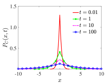
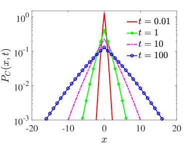
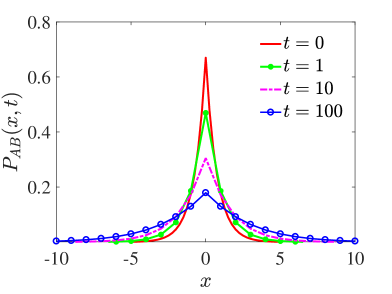
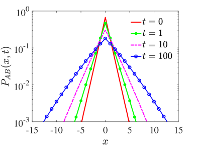
(a) (b)
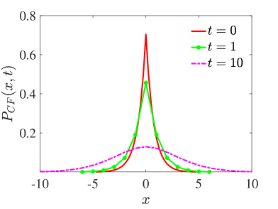
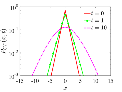
(c) (d)

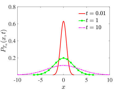
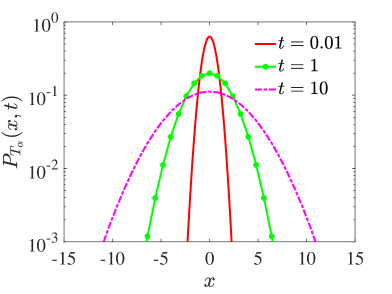
Figure 1: PDF of diffusion equations with initial condition $P(x,0)=\delta(x)$ with different integro-differential operators for $K_{\alpha}=1$, $\tau=1$, and $\alpha=0.5$: (a) Caputo-fractional, (b) Caputo-Fabrizio, (c) Atangana-Baleanu, and (d) Conformable. The solutions for the Caputo-FDE, CF-GDE and AB-GDE are obtained by applying an inverse Laplace transform to Eq. (32). Note that both PDFs for the CF- and AB-GDE have a Laplace shape with finite width at $t=0$. The solution (74) of the conformable diffusion equation is Gaussian at all times. The shapes are produced using Matlab code.

We digress briefly to shed some light on the delicate issue of placing specific forms of exponential tempering or other non-singular kernels in the integro-differential operators used above. We consider the case of the CF-operator. Let us use the Schneider-Wyss idea and start with the integral form (2) of the diffusion equation. We naively replace the integral on the right hand side with the operator (note that an analogous choice was made in Ref. lenzi )

$${}_{0}^{CF}D_{t}^{-\alpha}=\frac{\tau^{\alpha-1}}{1-\alpha}\int_{0}^{t}f(t^{\prime})\exp\left(-\frac{\alpha(t-t^{\prime})}{(1-\alpha)\tau}\right)dt^{\prime},$$ (60)

which is an integral operator with exponential tempering similar to the formulation of the CF-operator (8). Instead of the solution (30), for the initial condition $P_{0}(x)=\delta(x)$ we then obtain

$$P(k,s)=\frac{[\alpha/[(1-\alpha)\tau]+s]/s}{\alpha/[(1-\alpha)\tau]+s+K_{\alpha}\tau^{\alpha-1}k^{2}}.$$ (61)

The normalization is fulfilled, as for $k=0$ the Laplace transform reads $1/s$. The initial condition can be found from this equation by setting $s\to\infty$, which is $1/s$ to leading order. Inverse Fourier transform indeed reproduces the initial condition $P_{0}(x)=\delta(x)$.

The second moment is obtained by differentiation twice with respect to $k$ and setting $k=0$,

$$\langle x^{2}(t)\rangle=\frac{2K_{\alpha}\tau^{\alpha}(1-\alpha)}{\alpha}\left(1-\exp\left(-\frac{\alpha t}{(1-\alpha)\tau}\right)\right).$$ (62)

At short times we find normal diffusion,

$$\langle x^{2}(t)\rangle\sim 2K_{\alpha}\tau^{\alpha-1}t$$ (63)

with the effective diffusion coefficient $K_{\alpha}\tau^{\alpha-1}$, and at long times the saturation value

$$\langle x^{2}(t)\rangle\sim\frac{2(1-\alpha)K_{\alpha}\tau^{\alpha}}{\alpha}$$ (64)

is reached. This convergence to a stationary plateau is similar to what was observed previously for the tempering of FBM, that effected a behavior consistent with confinement daniel .

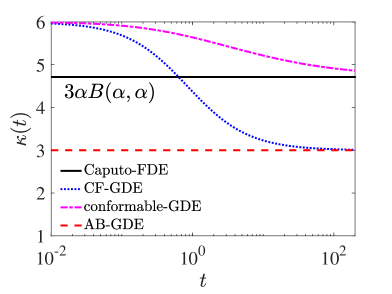
Figure 2: Kurtosis $\kappa$ for the GDE with different integro-differential operators for $K_{\alpha}=1$, $\tau=1$, and $\alpha=0.5$.

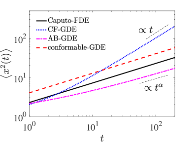
Figure 3: MSD for the GDEs with different integro-differential operators for $K_{\alpha}=1$, $\tau=1$, and $\alpha=0.5$.

The inverse Fourier transform of $P(k,s)$ becomes

$$P(x,s) = \frac{\sqrt{\pi\{\alpha/[(1-\alpha)\tau]+s\}/2}}{s\sqrt{K_{\alpha}\tau^{\alpha-1}}}$$ (65)

$$\times\exp\left(-\frac{|x|\sqrt{\alpha/[(1-\alpha)\tau]+s}}{\sqrt{K_{\alpha}\tau^{\alpha-1}}}\right).$$

At $s\to\infty$,

$$P(x,s) \sim \frac{1}{s}\lim_{s\to\infty}\sqrt{\frac{\pi/2}{K_{\alpha}\tau^{\alpha-1}/s}}\exp\left(-\frac{|x|\sqrt{s}}{\sqrt{K_{\alpha}\tau^{\alpha-1}}}\right)$$ (66)

$$\sim \frac{1}{s}\delta(x),$$

where we used the limiting form of the $\delta$-function. Thus, indeed, this form leads back to the consistent initial value. In the opposite long-time limit corresponding to $s\to 0$, we have

$$P(x,s)\sim\frac{1}{s}\sqrt{\frac{\pi/2}{K_{\alpha}\tau^{\alpha}(1-\alpha)/\alpha}}\exp\left(-\frac{|x|\sqrt{\alpha/(1-\alpha)}}{\sqrt{K_{\alpha}\tau^{\alpha}}}\right).$$ (67)

We thus have the stationary limit

$$P(x)\sim\sqrt{\frac{\pi/2}{K_{\alpha}\tau^{\alpha}(1-\alpha)/\alpha}}\exp\left(-\frac{|x|\sqrt{\alpha/(1-\alpha)}}{\sqrt{K_{\alpha}\tau^{\alpha}}}\right).$$ (68)

This is a Laplace distribution. We showed here for a simple modification of the integral form of the diffusion equation using a CF-type exponential tempering in the integral, how the time evolution of the PDF $P(x,t)$ will reach a non-trivial stationary value. Physically, this can be viewed as a consequence of introducing a finite time scale by the exponential factor in the integral. Beyond this time the contributions of the integral to the dynamics of $P(x,t)$ become exponentially small.

III.1.4 SBM and conformable diffusion equation

SBM in the absence of an external force, $F(x)=0$ in Eq. (19), and for the standard initial condition $P(x,0)=\delta(x)$ has the Gaussian shape lim2002self ; jeon2014scaled ,

$$P(x,t)=\frac{1}{\sqrt{4\pi K_{\alpha}t^{\alpha}}}\exp\left(-\frac{x^{2}}{4K_{\alpha}t^{\alpha}}\right),$$ (69)

with the associated MSD

$$\langle x^{2}(t)\rangle=2K_{\alpha}t^{\alpha}.$$ (70)

Concurrently, the GDE based on the conformable derivative is

$$T_{\alpha}P(x,t)=K_{\alpha}\frac{\partial^{2}}{\partial x^{2}}P(x,t).$$ (71)

For $P(x,0)=\delta(x)$ and after applying the conformable Laplace transform together with a Fourier transform

$$\mathscr{F}\{g(x)\}\equiv\int_{-\infty}^{\infty}g(x)\exp(ikx)dx,$$ (72)

we find

$$\hat{\tilde{P}}_{T_{\alpha}}(k,s)=\frac{1}{s+K_{\alpha}k^{2}}.$$ (73)

This directly leads to the PDF in $(x,t)$-space,

$$P_{T_{\alpha}}(x,t)=\sqrt{\frac{\alpha}{4\pi K_{\alpha}t^{\alpha}}}\exp\left(-\frac{\alpha x^{2}}{4K_{\alpha}t^{\alpha}}\right).$$ (74)

The Gaussianity of this PDF implies that the kurtosis is $\kappa_{T_{\alpha}}(t)=3$. The MSD encoded by the PDF (71) reads

$$\langle x^{2}(t)\rangle_{T_{\alpha}}=\frac{2K_{\alpha}}{\alpha}t^{\alpha}.$$ (75)

Thus, the conformable-GDE has the same PDF, MSD, and kurtosis as subdiffusive SBM. The PDF (74) of the conformable-GDE is displayed in Fig. 1 (d). The associated MSD and kurtosis are shown in Figs. 2 and 3. We will now show that the addition of a constant force (constant drift) allows one to distinguish between these two models.

III.2 Generalized Fokker-Planck equation with drift

From Sec. III.1.1 we conclude that the CF- and AB-operators in the formulation of the GDE (18) (for $F(x)=0$) do not provide a consistent formulation. We therefore do not consider them further here. We therefore limit our discussion of anomalous diffusion equation with drift to the Caputo, SBM, and conformable formulations.

III.2.1 Caputo diffusion equation with drift

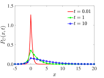
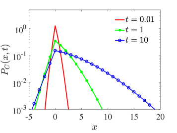
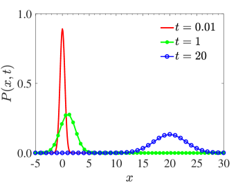
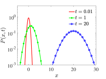
(a) (b) (c)

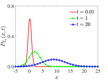
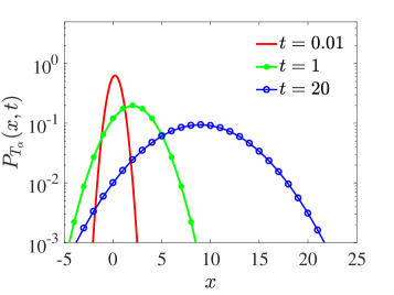
Figure 4: PDFs for drift-GDEs with initial condition $P(x,0)=\delta(x)$ of (a) Caputo, (b) SBM, (c) and conformable forms. We use the parameters $\alpha=0.5$, $v=v_{\alpha}=1$, and $K_{\alpha}=1$. Note that the position of the maximum of the PDF for the Caputo-FDE is stationary in space, corresponding to particles that have not moved up to time $t$. The maximum of the PDF for SBM with drift moves faster than that for the conformable-GDE.

The Caputo Fokker-Planck equation with drift reads (see also Ref. dieterich2015fluctuation )

$$^{C}_{0}D^{\alpha}_{t}[P(x,t)]=K_{\alpha}\frac{\partial^{2}}{\partial x^{2}}P(x,t)-v_{\alpha}\frac{\partial}{\partial x}P(x,t).$$ (76)

From the CTRW perspective, Eq. (76) appears as the diffusion (long time and space) limit of a walk with unequal probabilities to jump to the right and to the left mebakla1 ; igor_pre ; teza . In Laplace space the solution of Eq. (76) for the initial condition $P_{0}(x)=\delta(x)$ becomes

$$\tilde{P}_{C}(x,s) = \frac{s^{\alpha-1}}{\sqrt{v_{\alpha}^{2}+4K_{\alpha}s^{\alpha}}}$$ (77)

$$\times \exp\left(\frac{v_{\alpha}x}{2K_{\alpha}}-|x|\frac{\sqrt{v_{\alpha}^{2}+4K_{\alpha}s^{\alpha}}}{2K_{\alpha}}\right).$$

Applying a numerical inverse Laplace transformation to Eq. (77), we show this PDF in Fig. 4a.

The first moment and second moment encoded by the FDE (76) are

$$\langle x(t)\rangle_{C}=\frac{v_{\alpha}}{\Gamma(\alpha+1)}t^{\alpha}$$ (78)

and

$$\langle x^{2}(t)\rangle_{C}=\frac{2K_{\alpha}}{\Gamma(\alpha+1)}t^{\alpha}+\frac{2v_{\alpha}^{2}}{\Gamma(2\alpha+1)}t^{2\alpha}.$$ (79)

The MSD can then be calculated as

$$\langle(\Delta x)^{2}\rangle_{C} = \frac{2K_{\alpha}}{\Gamma(\alpha+1)}t^{\alpha}$$ (80)

$$+ \left[\frac{2}{\Gamma(2\alpha+1)}-\frac{1}{\Gamma(\alpha+1)^{2}}\right]v^{2}_{\alpha}t^{2\alpha}.$$

As well known from CTRW with a drift igor_pre ; scher ; report the MSD contains a term proportional to $v^{2}_{\alpha}t^{2\alpha}$, i.e., for $1/2<\alpha<1$ an effective superdiffusion occurs. This is due to the strong separation of particles stuck at the origin from mobile, advected particles.

III.2.2 SBM with drift and conformable diffusion equation with drift

The Fokker-Planck equation for SBM with drift is

$$\frac{\partial}{\partial t}P(x,t)=\mathscr{K}_{\alpha}(t)\frac{\partial^{2}}{\partial x^{2}}P(x,t)-v\frac{\partial}{\partial x}P(x,t),$$ (81)

from which we obtain the PDF

$$P(x,t)=\frac{1}{\sqrt{4\pi K_{\alpha}t^{\alpha}}}\exp\left(-\frac{(x-vt)^{2}}{4K_{\alpha}t^{\alpha}}\right),$$ (82)

which is shown in Fig. 4b. The associated moments are

$$\langle x(t)\rangle=vt,$$ (83)

$$\langle x^{2}(t)\rangle=2K_{\alpha}t^{\alpha}+v^{2}t^{2},$$ (84)

such that the MSD is

$$\langle(\Delta x)^{2}\rangle=2K_{\alpha}t^{\alpha}.$$ (85)

In contrast to the Caputo-FDE case, for SBM the Galilean invariance is preserved, giving rise to the similarity variable $x-vt$ in the PDF (82).

The GDE with drift based on the conformable derivative has the form

$$T_{\alpha}P(x,t)=K_{\alpha}\frac{\partial^{2}}{\partial x^{2}}P(x,t)-v_{\alpha}\frac{\partial}{\partial x}P(x,t).$$ (86)

Application of the conformable Laplace transform and Fourier transform yields

$$\hat{\tilde{P}}_{T_{\alpha}}(k,s)=\frac{1}{s+(K_{\alpha}k^{2}+iv_{\alpha}k)}.$$ (87)

From this form we obtain the PDF in $(x,t)$-space,

$$P_{T_{\alpha}}(x,t)=\sqrt{\frac{\alpha}{4\pi K_{\alpha}t^{\alpha}}}\exp\left(-\frac{\alpha(x-v_{\alpha}t^{\alpha}/\alpha)^{2}}{4K_{\alpha}t^{\alpha}}\right),$$ (88)

which is shown in Fig. 4c.

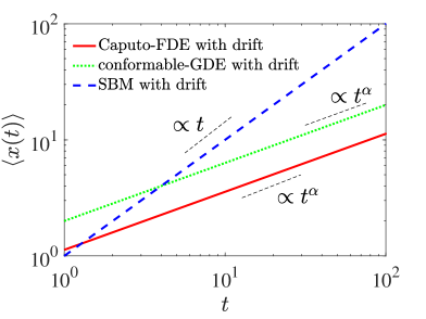
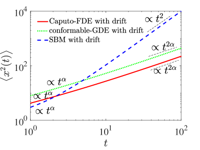
(a) (b) (c)

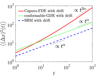
Figure 5: First (a) and (b) second moments, and (c) MSD for Caputo, conformable, and SBM forms. We chose $\alpha=0.5$, $v=v_{\alpha}=1$, and $K_{\alpha}=1$.

The associated first moment is

$$\langle x(t)\rangle=\frac{v_{\alpha}t^{\alpha}}{\alpha},$$ (89)

and the second moment reads

$$\langle x^{2}(t)\rangle=\frac{2K_{\alpha}}{\alpha}t^{\alpha}+\frac{v_{\alpha}^{2}}{\alpha^{2}}t^{2\alpha}.$$ (90)

The MSD is then

$$\langle(\Delta x)^{2}\rangle=\frac{2K_{\alpha}}{\alpha}t^{\alpha}.$$ (91)

The behaviors of the moments for the Caputo, SBM, and conformable forms of the generalized motion are shown in Fig. 5, from which one can distinguish SBM with drift from the Caputo and conformable drift-GDEs via the first moment: for SBM the first moment grows linearly in $t$, while for the other two cases a scaling with $t^{\alpha}$ occurs. From the MSD one can then distinguish the Caputo and conformable forms, respectively scaling as $t^{2\alpha}$ and $t^{\alpha}$ in the long time limit.

IV Generalized Langevin equations

We now turn to generalizations of the stochastic formulation of diffusive processes based on the Langevin equation, see daniel ; liemert2017generalized ; deng2009ergodic ; kou2004generalized ; porra1996generalized for details.

IV.1 Generalized Langevin equations in the force-free case

In the absence of an external force, $F(x)=0$, we consider formulations with different Caputo-, CF-, and AB-operators, SBM jeon2014scaled , and FBM jeon2010fractional ; mandelbrot1968fractional .

IV.1.1 Caputo and non-singular integro-differential operators

Applying the Caputo, CF- and AB-operators, we have the generalized Langevin equation,

$$\frac{d^{\alpha}}{dt^{\alpha}}x(t)=\sqrt{2K_{\alpha}}\xi(t),$$ (92)

for which we impose the initial condition $x(0)=0$. Here $d^{\alpha}/dt^{\alpha}$ represents the Caputo, CF- and AB-operators. Formal integration produces

$$x(t)=\sqrt{2K_{\alpha}}\int_{0}^{t}H(t-t^{\prime})\xi(t^{\prime})dt^{\prime},$$ (93)

where the integral kernel $H$ stands for

$$H_{C}(t) = \frac{t^{\alpha-1}}{\Gamma(\alpha)},$$

$$H_{CF}(t) = (1-\alpha)\tau^{\alpha}\delta(t)+\alpha\tau^{\alpha-1},$$

$$H_{AB}(t) = (1-\alpha)\tau^{\alpha}\delta(t)+\alpha\frac{t^{\alpha-1}}{\Gamma(\alpha)},$$ (94)

for the Caputo-, CF- and AB-operators, respectively.

(a)
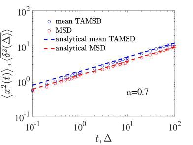
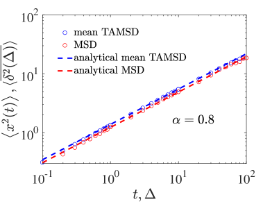
(b)
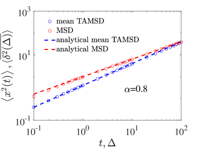
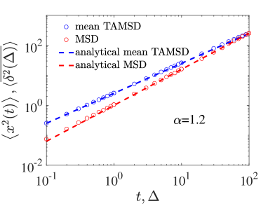
(c)

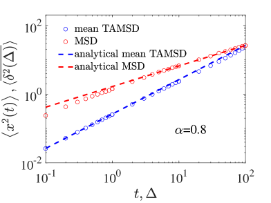
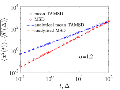
Figure 6: Simulations and analytical solutions for MSD and mean TAMSD for the (a) Caputo-, (b) SBM-, and (c) conformable-generalized Langevin equations, for $K_{\alpha}=0.5$.

For the Caputo-fractional Langevin equation, the two-point correlation function can be obtained in the form

$$\langle x(t_{1})x(t_{2})\rangle=\frac{2K_{\alpha}t_{2}^{\alpha}t_{1}^{\alpha-1}}{\alpha\Gamma{(\alpha)}^{2}}\,_{2}F_{1}\left(1-\alpha,1;\alpha+1;\frac{t_{2}}{t_{1}}\right),$$ (95)

where we assume (without limitation of generality) that $t_{1}\geq t_{2}$, and where

$${}_{2}F_{1}(a,b;c;z)=\frac{\Gamma(c)}{\Gamma(b)\Gamma(c-b)}\int_{0}^{1}\frac{t^{b-1}(1-t)^{c-b-1}}{(1-tz)^{a}}dt$$ (96)

is the hypergeometric function (see Eq. (166) in App B.2 for details of the derivation of Eq. (95)). From Eq. (95), the MSD follows for $t_{1}=t_{2}=t$, yielding

$$\langle x^{2}(t)\rangle=\frac{2K_{\alpha}}{(2\alpha-1)\Gamma{(\alpha)}^{2}}t^{2\alpha-1},$$ (97)

for $\alpha>1/2$ REM . We also obtain the mean TAMSD (see App C.1 for details) in the limit $\Delta/T\ll 1$,

$$\left<\overline{\delta^{2}(\Delta)}\right>\sim\frac{2K_{\alpha}}{\Gamma(2\alpha)\left|\cos(\pi\alpha)\right|}\Delta^{2\alpha-1}.$$ (98)

While the MSD and the mean TAMSD for the Caputo-Langevin equation thus have the same scaling exponent $2\alpha-1$, the two expressions have different prefactors. That implies that the process encoded by the Caputo-Langevin equation are non-ergodic in the Birkhoff-Boltzmann sense. In the notation of aljaz , we call such a case ultraweak ergodicity breaking. Results of stochastic simulations for the MSD and the mean TAMSD for the Caputo-Langevin equation are shown in Fig. 6a, and we find good agreement with the theoretical results. Details on the discrete simulations scheme for the different operators are provided in App D.

The fact that the Caputo-Langevin equation produces a non-stationary dynamics can be anticipated from the autocovariance function (95), see stas for further discussion. We finally report the displacement ACVF of this process, which asymptotically reads $C_{\Delta}(t)\sim[2(\alpha-1)K_{\alpha}/\{\alpha\Gamma^{2}(\alpha)\}]\Delta^{\alpha-1}t^{\alpha-2}$, see App C.2 for the derivation. We note that this behavior is different from the Caputo-FDE based on CTRW processes, for which the ACVF is zero beyond $t=\Delta$ stas .

For the case of the CF- and AB-Langevin equations we focus on their second moment,

$$\langle x^{2}(t)\rangle=2K_{\alpha}\int_{0}^{t}H^{2}(t^{\prime})dt^{\prime},$$ (99)

where for the kernel $H$ the respective forms from Eq. (94) should be substituted. Noticing that $\int_{0}^{t}\delta(t^{\prime})^{2}dt^{\prime}=\infty$, this means that the second moment for both CF- and AB-formulations diverges. Details of the derivations can be found in App B.2. Similar to our observations in the case of the FDE, the formulations in terms of the CF- and AB-operators lead to inconsistent results, and we will not pursue these operators further.

IV.1.2 SBM- and conformable-generalized Langevin equation

The formal solution of the SBM-Langevin equation (23) when $F(x)=0$ is

$$x(t)=\sqrt{2\alpha K_{\alpha}}\int_{0}^{t}(t^{\prime})^{\frac{\alpha-1}{2}}\xi(t^{\prime})dt^{\prime},$$ (100)

and the two-point correlation function reads

$$\langle x(t_{1})x(t_{2})\rangle=2K_{\alpha}[\min\{t_{1},t_{2}\}]^{\alpha}.$$ (101)

The MSD then has the power-law form jeon2014scaled

$$\langle x^{2}(t)\rangle=2K_{\alpha}t^{\alpha}.$$ (102)

The mean TAMSD grows as jeon2014scaled

$$\left<\overline{\delta^{2}(\Delta)}\right>=\frac{2K_{\alpha}\left[T^{\alpha+1}-\Delta^{\alpha+1}-(T-\Delta)^{\alpha+1}\right]}{(\alpha+1)(T-\Delta)}.$$ (103)

In the limit $\Delta/T\ll 1$,

$$\left<\overline{\delta^{2}(\Delta)}\right>\sim 2K_{\alpha}\Delta T^{\alpha-1},$$ (104)

which is linear in the lag time $\Delta$. SBM is thus weakly non-ergodic in the above Birkhoff-Boltzmann sense barkai2012single . In contrast to the ultraweak situation above, here the mean TAMSD explicitly depends on the measurement time $T$. Simulations results for the MSD and the mean TAMSD for SBM are shown in Fig. 6b.

The conformable Langevin equation

$$T_{\alpha}x(t)=\sqrt{2K_{\alpha}}\xi(t),$$ (105)

can be rephrased by using the relation $T_{\alpha}[f(t)]=t^{1-\alpha}df(t)/dt$ between the conformable derivative and the first order derivative,

$$\frac{d}{dt}x(t)=\sqrt{2K_{\alpha}}t^{\alpha-1}\xi(t),$$ (106)

and thus

$$x(t)=\sqrt{2K_{\alpha}}\int_{0}^{t}(t^{\prime})^{\alpha-1}\xi(t^{\prime})dt^{\prime}.$$ (107)

The two-point correlation function is

$$\langle x(t_{1})x(t_{2})\rangle=\frac{2K_{\alpha}}{2\alpha-1}[\min\{t_{1},t_{2}\}]^{2\alpha-1}.$$ (108)

for $\alpha>1/2$. Finally, the MSD becomes

$$\langle x^{2}(t)\rangle=\frac{2K_{\alpha}}{2\alpha-1}t^{2\alpha-1}.$$ (109)

For the mean TAMSD we obtain

$$\left<\overline{\delta^{2}(\Delta)}\right>=\frac{C_{1}}{2\alpha}\frac{T^{2\alpha}}{T-\Delta}\left[1-\left(\frac{\Delta}{T}\right)^{2\alpha}-\left(1-\frac{\Delta}{T}\right)^{2\alpha}\right],$$ (110)

where $C_{1}=2K_{\alpha}/[(2\alpha-1)\Gamma^{2}(\alpha)].$ In the limit $\Delta/T\ll 1$,

$$\left<\overline{\delta^{2}(\Delta)}\right>\sim\frac{K_{\alpha}}{2\alpha-1}\Delta T^{2\alpha-2}.$$ (111)

The conformable-Langevin equation encodes a weakly non-ergodic and non-stationary dynamic. Simulations results of the MSD and mean TAMSD for the conformable-Langevin equation (105) with different $\alpha$ are shown in Fig. 6c. From Eqs. (101) and (108) it follows that both processes, SBM and conformable-Langevin equation motion have independent increments, and thus the ACVFs defined in Eq. (27) vanishes for these processes, $C_{\Delta}(t)=0$. The analysis of the MSDs (102) and (109) for the two processes shows that they have the same time-scaling if we take the exponent $\alpha$ for SBM equal to the exponent $2\alpha-1$ for the conformable-Langevin equation. A similar conclusion follows from Eqs. (104) and (111). Therefore, the information encoded in the MSD and mean TAMSD is insufficient to distinguish between these two processes. Analogously to the situation considered in Section III.2 for the SBM- and conformable-diffusion equations we will show that adding a constant force (constant drift) allows us to distinguish between these two Langevin models.

IV.1.3 FBM

The formal solution of FBM for $F(x)=0$ is (24)

$$x(t)=\int_{0}^{t}\xi_{\alpha}(t^{\prime})dt^{\prime},$$ (112)

with the two-point correlation

$$\langle x(t_{1})x(t_{2})\rangle=K_{\alpha}\left(t_{1}^{\alpha}+t_{2}^{\alpha}-\left|t_{1}-t_{2}\right|^{\alpha}\right).$$ (113)

Thus, the MSD has the power-law form

$$\langle x^{2}(t)\rangle=2K_{\alpha}t^{\alpha}.$$ (114)

The mean TAMSD of FBM is deng2009ergodic

$$\left<\overline{\delta^{2}(\Delta)}\right>=2K_{\alpha}\Delta^{\alpha}.$$ (115)

We conclude that this free FBM is ergodic and stationary. Finally, the normalized autocovariance of FBM can be represented as $C_{\Delta}(t)/C_{\Delta}(0)=[(t+\Delta)^{\alpha}-2t^{\alpha}+|t-\Delta|^{\alpha}/[2\Delta^{\alpha}]$, for $\Delta\neq 0$ jae .

IV.2 Generalized Langevin equations with drift

IV.2.1 Caputo-fractional Langevin equation with drift

The Caputo-fractional Langevin equation with drift reads

$${}^{C}_{0}D^{\alpha}_{t}x(t)=\sqrt{2K_{\alpha}}\xi(t)+v_{\alpha}.$$ (116)

After a Laplace transformation,

$$\tilde{x}(s)=\frac{v_{\alpha}}{s^{1+\alpha}}+\sqrt{2K_{\alpha}}\frac{\xi(s)}{s^{\alpha}}.$$ (117)

Back-transforming to the time domain,

$$x(t)=\frac{v_{\alpha}t^{\alpha}}{\Gamma(1+\alpha)}+\sqrt{2K_{\alpha}}\int_{0}^{t}\frac{{(t-t^{\prime})}^{\alpha-1}}{\Gamma(\alpha)}\xi(t^{\prime})dt^{\prime}.$$ (118)

The first moment is then given by

$$\langle x(t)\rangle=\frac{v_{\alpha}t^{\alpha}}{\Gamma(1+\alpha)},$$ (119)

which coincides with the result (78) of the Caputo-FDE. Similar to the derivation of Eq. (95), the two-point correlation function of the Caputo-fractional Langevin equation in the presence of a drift is

$$\langle x(t_{1})x(t_{2})\rangle = \frac{v_{\alpha}^{2}}{\Gamma^{2}(1+\alpha)}(t_{1}t_{2})^{\alpha}+\frac{2K_{\alpha}t_{2}^{\alpha}t_{1}^{\alpha-1}}{\alpha\Gamma{(\alpha)}^{2}}$$ (120)

$$\times\,_{2}F_{1}\left(1-\alpha,1,\alpha+1,\frac{t_{2}}{t_{1}}\right),$$

where we assumed that $t_{1}<t_{2}$. The second moment is

$$\langle x^{2}(t)\rangle=\frac{v_{\alpha}^{2}}{\Gamma^{2}(1+\alpha)}t^{2\alpha}+\frac{2K_{\alpha}}{(2\alpha-1)\Gamma^{2}(\alpha)}t^{2\alpha-1},\alpha>\frac{1}{2}.$$ (121)

for $\alpha>1/2$. We finally obtain the MSD

$$\langle(\Delta x)^{2}(t)\rangle=\frac{2K_{\alpha}}{(2\alpha-1)\Gamma^{2}(\alpha)}t^{2\alpha-1}.$$ (122)

The forms of the second moment (121) and the MSD (122) are different from their counterparts (79) and (80) for the Caputo-FDE. In the Caputo-fractional Langevin equation the drift enters additively and is not affected by the memory in the fractional operator. In contrast, for the Caputo-FDE the particles are immobilized during the waiting times represented by the fractional operator.

IV.2.2 SBM- and conformable-Langevin equations with drift

The SBM-Langevin equation with drift has the form

$$\frac{d}{dt}x(t)=\sqrt{2K_{\alpha}(t)}\xi(t)+v.$$ (123)

The moments are readily calculated, yielding

$$\langle x(t)\rangle=vt$$ (124)

and

$$\langle x^{2}(t)\rangle=2K_{\alpha}t^{\alpha}+v^{2}t^{2}.$$ (125)

Thus the MSD is

$$\langle(\Delta x)^{2}\rangle=2K_{\alpha}t^{\alpha}.$$ (126)

The conformable-Langevin equation with drift is

$$T_{\alpha}x(t)=\sqrt{2K_{\alpha}}\xi(t)+v_{\alpha}.$$ (127)

With the relation $T_{\alpha}f(t)=t^{1-\alpha}df(t)/dt$, we obtain

$$\frac{d}{dt}x(t)=t^{\alpha-1}\left(\sqrt{2K_{\alpha}}\xi(t)+v_{\alpha}\right),$$ (128)

and thus

$$x(t) = \int_{0}^{t}(t^{\prime})^{\alpha-1}\left(\sqrt{2K_{\alpha}}\xi(t^{\prime})+v_{\alpha}\right)dt^{\prime}$$ (129)

$$= \frac{v_{\alpha}}{\alpha}t^{\alpha}+\sqrt{2K_{\alpha}}\int_{0}^{t}(t^{\prime})^{\alpha-1}\xi(t^{\prime})dt^{\prime},$$

and thus the first moment is equivalent to the deterministic form

$$\langle x(t)\rangle=\frac{v_{\alpha}}{\alpha}t^{\alpha}.$$ (130)

The two-point correlation function becomes

$$\langle x(t_{1})x(t_{2})\rangle=\frac{v_{\alpha}^{2}}{\alpha^{2}}(t_{1}t_{2})^{\alpha}+\frac{2K_{\alpha}}{2\alpha-1}t_{2}^{2\alpha-1}.$$ (131)

valid for $\alpha>1/2$. The second moment follows as

$$\langle x^{2}(t)\rangle=\frac{v_{\alpha}^{2}}{\alpha^{2}}t^{2\alpha}+\frac{2K_{\alpha}}{2\alpha-1}t^{2\alpha-1}.$$ (132)

Finally, the MSD has the $v_{\alpha}$-independent form

$$\langle(\Delta x)^{2}(t)\rangle=\frac{2K_{\alpha}}{2\alpha-1}t^{2\alpha-1}$$ (133)

for $\alpha>1/2$. One can see from Eqs. (124) and (130) that the response to a constant force is different for SBM-Langevin and conformable-Langevin equations, thus allowing us to distinguish between these two anomalous diffusion models.

IV.2.3 FBM with drift

We finally consider the FBM Langevin equation with drift,

$$x(t)=\int_{0}^{t}dt^{\prime}\xi_{\alpha}(t^{\prime})+vt,$$ (134)

such that

$$\langle x(t)\rangle=vt.$$ (135)

The two-point correlation behaves as

$$\langle x(t_{1})x(t_{2})\rangle=K_{\alpha}\left(t_{1}^{\alpha}+t_{2}^{\alpha}-|t_{1}-t_{2}|^{\alpha}\right)+v^{2}t_{1}t_{2}.$$ (136)

The second moment encoded in this form is

$$\langle x^{2}(t)\rangle=2K_{\alpha}t^{\alpha}+v^{2}t^{2}.$$ (137)

Finally, the MSD reads

$$\langle(\Delta x)^{2}(t)\rangle=2K_{\alpha}t^{\alpha}.$$ (138)

The moments for the different processes are shown in Fig. 7. From the above discussion we see that the first moments of the Caputo-fractional and and conformable-Langevin equations with drift have a power-law form, which is distinct from the linear time dependence in the SBM- and FBM-Langevin equations.

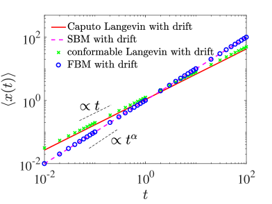
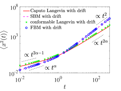
(a) (b) (c)

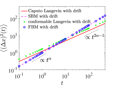
Figure 7: First (a) and second (b) moments and (c) MSD for Caputo-fractional, conformable-, SBM-, and FBM-Langevin equations with drift for $v=1$, $\alpha=0.8$, and $K_{\alpha}=0.5$. Note that the results of SBM and FBM fully coincide in all three panels.

Fokker-Planck Eq.		Caputo $(0<\alpha\leq 1)$	conformable $(0<\alpha\leq 1)$	SBM $(\alpha>0)$
$F(x)=0$	$P(x,t)$	$\frac{1}{2\sqrt{K_{\alpha}t^{\alpha}}}M_{\frac{\alpha}{2}}\left(\frac{|x|}{\sqrt{K_{\alpha}t^{\alpha}}}\right)$	$\sqrt{\frac{\alpha}{4\pi K_{\alpha}t^{\alpha}}}\exp\left(-\frac{\alpha x^{2}}{4K_{\alpha}t^{\alpha}}\right)$	$\frac{1}{\sqrt{4\pi K_{\alpha}t^{\alpha}}}\exp\left(-\frac{x^{2}}{4K_{\alpha}t^{\alpha}}\right)$
	$\langle x^{2}(t)\rangle$	$\frac{2K_{\alpha}}{\Gamma(\alpha+1)}t^{\alpha}$	$\frac{2K_{\alpha}}{\alpha}t^{\alpha}$	$2K_{\alpha}t^{\alpha}$
$F(x)=v$	$P(x,t)$	$\mathscr{L}^{-1}[\tilde{P}_{C}(x,s)]$	$\sqrt{\frac{\alpha}{4\pi K_{\alpha}t^{\alpha}}}\exp\left(-\frac{\alpha(x-\frac{v_{\alpha}t^{\alpha}}{\alpha})^{2}}{4K_{\alpha}t^{\alpha}}\right)$	$\frac{1}{\sqrt{4\pi K_{\alpha}t^{\alpha}}}\exp\left(-\frac{(x-vt)^{2}}{4K_{\alpha}t^{\alpha}}\right)$
	$\langle x(t)\rangle$	$\frac{v_{\alpha}}{\Gamma(\alpha+1)}t^{\alpha}$	$v_{\alpha}\frac{t^{\alpha}}{\alpha}$	$vt$
	$\langle x^{2}(t)\rangle$	$\frac{2K_{\alpha}}{\Gamma(\alpha+1)}t^{\alpha}+\frac{2v_{\alpha}^{2}}{\Gamma(2\alpha+1)}t^{2\alpha}$	$\frac{2K_{\alpha}}{\alpha}t^{\alpha}+\frac{v_{\alpha}^{2}}{\alpha^{2}}t^{2\alpha}$	$2K_{\alpha}t^{\alpha}+v^{2}t^{2}$
	$\langle(\Delta x)^{2}(t)\rangle$	$\frac{2K_{\alpha}}{\Gamma(\alpha+1)}t^{\alpha}+at^{2\alpha}$	$\frac{2K_{\alpha}}{\Gamma(\alpha+1)}t^{\alpha}$	$2K_{\alpha}t^{\alpha}$

Table 1: Central results for the displacement PDFs and moments of the generalized Fokker-Planck equations with Caputo-fractional and conformable derivatives and SBM for the cases without and with drift.

Langevin Eq.		Caputo $(\frac{1}{2}<\alpha\leq 1)$	conformable $(\frac{1}{2}<\alpha\leq 1)$	SBM $(\alpha>0)$	FBM $(0<\alpha<2)$
$F(x)=0$	$\langle x^{2}(t)\rangle$	$\frac{2K_{\alpha}}{(2\alpha-1)\Gamma(\alpha)^{2}}t^{2\alpha-1}$	$\frac{2K_{\alpha}}{2\alpha-1}t^{2\alpha-1}$	$2K_{\alpha}t^{\alpha}$	$2K_{\alpha}t^{\alpha}$
	$\left<\overline{\delta^{2}(\Delta)}\right>$	$\sim\frac{2K_{\alpha}}{\Gamma(2\alpha)\left|\cos(\pi\alpha)\right|}\Delta^{2\alpha-1}$	$\sim\frac{K_{\alpha}}{2\alpha-1}\Delta T^{2\alpha-2}$	$\sim 2K_{\alpha}\Delta T^{\alpha-1}$	$2K_{\alpha}\Delta^{\alpha}$
	$C_{\Delta}(t),\,t\gg\Delta$	$\simeq(\alpha-1)K_{\alpha}\Delta^{\alpha-1}t^{\alpha-2}$	$0$	$0$	$\simeq(\alpha-1)\Delta^{\alpha-2}$
$F(x)=v,v_{\alpha}$	$\langle x(t)\rangle$	$v_{\alpha}\frac{t^{\alpha}}{\Gamma(1+\alpha)}$	$v_{\alpha}\frac{t^{\alpha}}{\alpha}$	$vt$	$vt$
	$\langle x^{2}(t)\rangle$	$\frac{v_{\alpha}^{2}}{\Gamma(1+\alpha)^{2}}t^{2\alpha}+\frac{2K_{\alpha}}{(2\alpha-1)\Gamma(\alpha)^{2}}t^{2\alpha-1}$	$\frac{v_{\alpha}^{2}}{\alpha^{2}}t^{2\alpha}+\frac{2K_{\alpha}}{2\alpha-1}t^{2\alpha-1}$	$2K_{\alpha}t^{\alpha}+v^{2}t^{2}$	$2K_{\alpha}t^{\alpha}+v^{2}t^{2}$
	$\langle(\Delta x)^{2}(t)\rangle$	$\frac{2K_{\alpha}}{(2\alpha-1)\Gamma(\alpha)^{2}}t^{2\alpha-1}$	$\frac{2K_{\alpha}}{2\alpha-1}t^{2\alpha-1}$	$2K_{\alpha}t^{\alpha}$	$2K_{\alpha}t^{\alpha}$

Table 2: Central results for the moments, mean TAMSD, and autocovariance function of the generalized Langevin equations with Caputo-fractional and conformable derivatives, SBM and FBM, without and with drift.

V Conclusions

Fractional dynamic equations of the relaxation and diffusion types have been used in science and engineering for considerable time. Traditionally, these generalized equations were used in the Riemann-Liouville and Caputo types. These are particularly suitable for the formulation of initial value problems posed at $t=0$. Other formulations such as the Weyl-Riesz forms have been used, as well, e.g., in the context of generalized rheological models for harmonic driving helmut ; helmut1 . More recently, additional definitions of fractional and conformable operators have been proposed and discussed in literature. We here studied generalized diffusion and Langevin equations, comparing the classical Caputo-fractional forms with the CF-, AB-, and conformable-generalized differential operators. We also compare these results to two other anomalous diffusion processes, SBM and FBM.

In our analysis we find that the formulations in terms of the CF- and AB-operators lead to inconsistent results for the PDFs and MSDs in both the GDE and generalized Langevin equation cases. While this point requires further analysis from a more mathematical point of view, we here did not pursue the formulations in terms of these operators further. A possible solution for the incorrect incorporation of the initial values for these two operators in the traditional formulation (note that the integral formulation as outlined in the Introduction for the CF- and AB-cases produces the same results) may be that instead of an initial condition at $t=0$, the initial condition has to be formulated on an interval. We discussed an alternative formulation similar to the CF-GDE in which the initial condition is consistently incorporated. The latter formulation will deserve further analysis in the future.

Results for the moments, the MSD, and the PDF of the different formulations using Caputo-fractional, conformable-, SBM-, and FBM-dynamic equations are summarized in Tabs. 1 and 2. Generally we see that the first moments in the presence of drift are identical for both GDE and Langevin formulations for each of the Caputo-, conformable-, and SBM-models, while their higher order moments are different between GDE and Langevin descriptions for the Caputo and conformable cases. The Caputo-, conformable-, and SBM-cases exhibit non-stationarity and non-ergodic behavior. The PDFs are Gaussian in all cases apart from the Caputo-FDE. We also see that by combining moments in the presence and absence of a constant drift velocity the three models can be distinguished.

Of particular interest here is the formulation in terms of the conformable derivative. The resulting PDF turns out to be the same as the PDF for SBM in the force-free case, after a renormalization of the generalized diffusion coefficient. In the presence of a drift, both processes differ in the scaling of the first moment and in the form the drift enters the PDF. Despite its "local" definition, the conformable-GDE is weakly non-ergodic and shows aging properties. These effects are visible in the comparison of the MSD with the mean TAMSD as well as in the two-point correlation function in the conformable-Langevin equation case.

We also note that we chose to present our analysis in dimensional units. This requires the use of generalized diffusion coefficients and drift velocities. Including dimensionality allows for an explicit extraction of the parameters from measurements. It also demonstrates the different ways (local or with a generalized exponent) the drift enters the different model dynamics.

Our study should help to assess and compare different formulations of GDEs and generalized Langevin equations. A similar analysis should be performed for the case of a harmonic confinement of the test particle. Moreover, different forms of crossovers to normal dynamics should be studied.

Appendix A Integral versions of CF- and AB-operators

To find the inverse operator of Eq. (8), the CF-integral, we take $0<\alpha\leq 1$ and consider the equation

$${}^{CF}_{0}D^{\alpha}_{t}f(t)=u(t).$$ (139)

After a Laplace transform we obtain

$$\mathscr{L}\{f(t)\}(s) = \frac{1}{s}f(0)+\frac{\alpha\tau^{\alpha-1}}{sM(\alpha)}\mathscr{L}\{u(t)\}(s)$$ (140)

$$+\frac{(1-\alpha)\tau^{\alpha}}{M(\alpha)}\mathscr{L}\{u(t)\}(s).$$

Rearranging and after inverse Laplace transformation we deduce that

$$f(t)=\frac{(1-\alpha)\tau^{\alpha}}{M(\alpha)}u(t)+\frac{\alpha\tau^{\alpha-1}}{M(\alpha)}\int_{0}^{t}u(s)ds+f(0).$$ (141)

Thus, the CF-integral is defined as

$${}_{0}^{CF}I_{t}^{\alpha}u(t)=\frac{(1-\alpha)\tau^{\alpha}}{M(\alpha)}u(t)+\frac{\alpha\tau^{\alpha-1}}{M(\alpha)}\int_{0}^{t}u(s)ds.$$ (142)

Similarly, the modified AB-integral corresponding to the operator (10) is

$${}_{0}^{AB}\mathrm{I}_{t}^{\alpha}f(t) = \frac{(1-\alpha)}{B(\alpha)}\tau^{\alpha}f(t)$$ (143)

$$+ \frac{\alpha}{B(\alpha)\Gamma(\alpha)}\int_{0}^{t}f(t^{\prime})(t-t^{\prime})^{\alpha-1}dt^{\prime},$$

for $0<\alpha\leq 1$.

Appendix B Integro-differential operators in diffusion and Langevin equations

B.1 Integro-differential operators in diffusion equations

For the Caputo-FDE the PDF (36) can also be represented in terms of the Fox $H$-function mathai

$$P_{C}(x,t)=\frac{1}{\sqrt{4K_{\alpha}t^{\alpha}}}H_{1,1}^{1,0}\left[\frac{|x|}{\sqrt{K_{\alpha}t^{\alpha}}}\left|\begin{array}[]{l}(1-\alpha/2,\alpha/2)\\ (0,1)\end{array}\right.\right].$$ (144)

For the PDFs of the CF- and AB-GDEs, we check whether their PDFs in Laplace space are completely monotonic Rschilling2010 . To this end we first check the complete monotonicity of expressions (32), (34), and (35). First, we introduce the completely monotone functions (CMF) and Bernstein functions (BF), as well as some useful properties of these two types of functions. CMFs can be represented as Laplace transforms of a non-negative function $p(t)$, i.e., $m(x)=\int_{0}^{\infty}p(t)\exp{(-xt)}dt$. They are defined on the non-negative half-axis and have the property that $(-1)^{n}m^{(n)}(x)\geq 0$ for all $n\in\mathbb{N}_{0}$ and $x\geq 0$. The following property holds true for CMFs Rschilling2010 :

(i) The product $m(x)=m_{1}(x)m_{2}(x)$ of two CMFs $m_{1}(x)$ and $m_{2}(x)$ is again a CMF.

The Bernstein functions Rschilling2010 are non-negative functions, whose derivative is completely monotone. They have the property that $(-1)^{(n-1)}b^{(n)}(x)\geq 0$, for all $n=\mathbb{N}$. The Bernstein functions have the following two properties:

(ii) A composition $b_{1}\big{(}b_{2}(s)\big{)}$ of Bernstein functions is again a Bernstein function.

(iii) A composition $m\big{(}b(x)\big{)}$ of a CMF $m(x)$ and a Bernstein function $b(x)$ is a CMF.

From these properties it follows that the function $\exp(-ub(x))$ is completely monotone for $u>0$ if $b(x)$ is a Bernstein function.

Now let $f_{1}(s)=1/\sqrt{s(c_{1}s+c_{2})}=1/[\sqrt{s}\sqrt{c_{1}s+c_{2}}]$. As $1/\sqrt{s}$ is a CMF, $1/\sqrt{c_{1}s+c_{2}}$ is a CMF, so from property (i) $f_{1}(s)$ is also a CMF. Let $f_{2}(s)=\exp(-\sqrt{s/(c_{1}s+c_{2})}|x|)$. As $\sqrt{s}$ is a BF and $s/(c_{1}s+c_{2})$ is a BF, then from property (ii), $\sqrt{s/(c_{1}s+c_{2})}$ is a BF. As $\exp(-s)$ is a CMF, then from property (iii), $f_{2}(s)$ is a CMF. Consequently $\tilde{P}_{CF}(x,s)=f_{1}(s)f_{2}(s)$ is a CMF. Similarly, $\tilde{P}_{AB}(x,s)$ is a CMF. From the above we can ensure that the PDFs of the CF- and AB-GDEs obtained from Eqs. (32), (34) and (35) represent proper PDFs.

Now we focus on the calculation of the second moment from the GDE (28),

$$\langle x^{2}(t)\rangle=\int_{-\infty}^{\infty}x^{2}P(x,t)dx,$$ (145)

with initial value $\langle x^{2}(0)\rangle=\int_{-\infty}^{\infty}x^{2}P(x,0)dx=0$ for $P(x,0)=\delta(x)$. It then follows that

$$\frac{d^{\alpha}}{dt^{\alpha}}\langle x^{2}(t)\rangle=K_{\alpha}\int_{-\infty}^{\infty}x^{2}\left[\frac{\partial^{2}}{\partial x^{2}}P(x,t)\right]dx=2K_{\alpha}.$$ (146)

Applying a Laplace transformation to Eq. (146),

$$\mathscr{L}\left[\frac{d^{\alpha}}{dt^{\alpha}}\langle x^{2}(t)\rangle\right]=2K_{\alpha}\frac{1}{s}.$$ (147)

For the Caputo-derivative,

$$s^{\alpha}\left\langle\tilde{x}^{2}(s)\right\rangle_{C}=2D_{\alpha}\frac{1}{s},$$ (148)

and the second moment becomes

$$\langle x^{2}(t)\rangle=\frac{2K_{\alpha}}{\Gamma(\alpha+1)}t^{\alpha},$$ (149)

which is a familiar results report .

For the CF-GDE,

$$\frac{s}{(1-\alpha)s+\alpha}\langle\tilde{x}^{2}(s)\rangle_{CF}=2K_{\alpha}\frac{1}{s},$$ (150)

such that

$$\langle\tilde{x}_{(s)}^{2}\rangle=2K_{\alpha}(1-\alpha)\frac{1}{s}+2K_{\alpha}\alpha\frac{1}{s^{2}},$$ (151)

and then

$$\langle x^{2}(t)\rangle_{CF}=2K_{\alpha}(1-\alpha)+2K_{\alpha}\alpha t.$$ (152)

For the AB-GDE,

$$\frac{s^{\alpha}}{(1-\alpha)s^{\alpha}+\alpha}\langle\tilde{x}^{2}(s)\rangle=2K_{\alpha}\frac{1}{s},$$ (153)

such that

$$\langle\tilde{x}^{2}(s)\rangle=2K_{\alpha}(1-\alpha)\frac{1}{s}+2K_{\alpha}\alpha\frac{1}{s^{\alpha+1}},$$ (154)

and then

$$\langle x^{2}(t)\rangle_{AB}=2K_{\alpha}(1-\alpha)+2K_{\alpha}\frac{t^{\alpha}}{\Gamma{(\alpha)}}.$$ (155)

For the kurtosis, we calculate the third and fourth order moments,

$$\langle x^{3}(s)\rangle = -i\left.\frac{\partial^{3}}{\partial k^{3}}\hat{\tilde{P}}(k,s)\right|_{k=0},$$ (156)

$$\langle x^{4}(s)\rangle = \left.\frac{\partial^{4}}{\partial k^{4}}\hat{\tilde{P}}(k,s)\right|_{k=0}.$$ (157)

From these we find the kurtosis

$$\kappa(t)=\left<\left(\frac{x-\langle x\rangle}{\left<\left(x-\langle x\rangle\right)^{2}\right>^{1/2}}\right)^{4}\right>.$$ (158)

The kurtosis for the CF- and AB-GDEs are

$$\kappa_{CF}=6\left[\frac{(1-\alpha)+\alpha\frac{t}{\sqrt{2}}}{(1-\alpha)+\alpha t}\right]^{2},$$ (159)

and

$$\kappa_{AB}=6\frac{\frac{\alpha t^{2\alpha}}{2\Gamma{(2\alpha)}}+2(1-\alpha)\frac{t^{\alpha}}{\Gamma{(\alpha)}}+(1-\alpha)^{2}}{\left[\frac{t^{\alpha}}{\Gamma{(\alpha)}}+(1-\alpha)\right]^{2}}.$$ (160)

B.2 Integro-differential operators in the Langevin equation

The generalized Langevin equation with integro-differential operators is

$$\frac{d^{\alpha}}{dt^{\alpha}}x(t)=\sqrt{2K_{\alpha}}\xi(t),$$ (161)

where $0<\alpha\leq 1$ and $d^{\alpha}/dt^{\alpha}$ represents the Caputo-, CF- and AB-operators. Applying a Laplace transformation,

$$\tilde{x}(s)=\sqrt{2K_{\alpha}}\frac{1}{s\tilde{\theta}(s)}\tilde{\xi}(s),$$ (162)

where $\theta_{C}(t)=\frac{t^{-\alpha}}{\Gamma(1-\alpha)}$, $\theta_{CF}(t)=\frac{1}{(1-\alpha)\tau^{\alpha}}\exp{\left(-\frac{\alpha t}{(1-\alpha)\tau}\right)}$, $\theta_{AB}(t)=\frac{1}{(1-\alpha)\tau^{\alpha}}E_{\alpha}\left(-\alpha\frac{t^{\alpha}}{(1-\alpha)\tau^{\alpha}}\right)$. After inverse Laplace transformation, we obtain

$$x(t)=\sqrt{2K_{\alpha}}\int_{0}^{t}H(t-t^{\prime})\xi(t^{\prime})dt^{\prime}.$$ (163)

The MSD is then

$$\langle x^{2}(t)\rangle=2K_{\alpha}\int_{0}^{t}H^{2}(t^{\prime})dt^{\prime}.$$ (164)

Here, $H_{CF}(t)=(1-\alpha)\tau^{\alpha}\delta(t)+\alpha\tau^{\alpha-1}$, and $H_{AB}(t)=(1-\alpha)\tau^{\alpha}\delta(t)+\alpha\frac{t^{\alpha-1}}{\Gamma(\alpha)}$.

For the Caputo derivative,

$$x(t)=\sqrt{2K_{\alpha}}\int_{0}^{t}\frac{(t-t^{\prime})^{\alpha-1}}{\Gamma(\alpha)}\xi(t^{\prime})dt^{\prime}.$$ (165)

The two-point correlation function for the Caputo-fractional Langevin equation is

$$\langle x(t_{1})x(t_{2})\rangle = 2K_{\alpha}\int_{0}^{t_{1}}\frac{(t_{1}-t_{1}^{\prime})^{\alpha-1}}{\Gamma(\alpha)}dt_{1}^{\prime}$$ (166)

$$\times\int_{0}^{t_{2}}\frac{(t_{2}-t_{2}^{\prime})^{\alpha-1}}{\Gamma(\alpha)}dt_{2}^{\prime}\langle\xi(t_{1}^{\prime})\xi(t_{2}^{\prime})\rangle$$

$$=\frac{2K_{\alpha}}{\Gamma{(\alpha)}^{2}}\int_{0}^{t_{1}}(t_{1}-t_{1}^{\prime})^{\alpha-1}dt_{1}^{\prime}$$

$$\times\int_{0}^{t_{2}}(t_{2}-t_{2}^{\prime})^{\alpha-1}dt_{2}^{\prime}\delta(t_{1}^{\prime}-t_{2}^{\prime})$$

$$=\frac{2K_{\alpha}}{\Gamma{(\alpha)}^{2}}\int_{0}^{t_{2}}(t_{1}-t_{2}^{\prime})^{\alpha-1}(t_{2}-t_{2}^{\prime})^{\alpha-1}dt_{2}^{\prime}$$

$$=\frac{2K_{\alpha}}{\Gamma{(\alpha)}^{2}}t_{2}^{\alpha}t_{1}^{\alpha-1}\int_{0}^{1}(1-\frac{t_{2}}{t_{1}}x)^{\alpha-1}(1-x)^{\alpha-1}dx$$

$$=\frac{2K_{\alpha}t_{2}^{\alpha}t_{1}^{\alpha-1}}{\alpha\Gamma{(\alpha)}^{2}}\,_{2}F_{1}\left(1-\alpha,1;\alpha+1;\frac{t_{2}}{t_{1}}\right).$$

Without restricting generality, we here assume that $t_{1}\geq t_{2}$, and

$${}_{2}F_{1}(a,b;c;z)=\frac{\Gamma(c)}{\Gamma(b)\Gamma(c-b)}\int_{0}^{1}\frac{t^{b-1}(1-t)^{c-b-1}}{(1-tz)^{a}}dt$$ (167)

is the hypergeometric function, which for $|z|<1$ is defined by the power series

$$_{2}F_{1}(a,b;c;z)=\sum_{n=0}^{\infty}\frac{(a)_{n}(b)_{n}}{(c)_{n}}\frac{z^{n}}{n!}.$$ (168)

Here $(q)_{n}$ is the (rising) Pochhammer symbol

$$(q)_{n}=\left\{\begin{array}[]{ll}1,&n=0\\ q(q+1)\cdots(q+n-1),&n>0\end{array}\right..$$

Then the MSD is

$$\langle x^{2}(t)\rangle=C_{1}t^{2\alpha-1},$$ (169)

for $\alpha>1/2$, and where $C_{1}=2K_{\alpha}/[(2\alpha-1)\Gamma^{2}(\alpha)]$.

Appendix C TAMSD and ACVF for Caputo Langevin equation

C.1 TAMSD

According to the definition (25) of the TAMSD, the mean TAMSD of the Caputo-fractional Langevin equation can be derived in the form

$$\left<\overline{\delta^{2}(\Delta)}\right> = \left<\frac{1}{T-\Delta}\int_{0}^{T-\Delta}\left[x(t+\Delta)-x(t)\right]^{2}dt\right>$$ (170)

$$=\frac{1}{T-\Delta}\int_{0}^{T-\Delta}\left[\langle x^{2}(t+\Delta)\rangle+\langle x^{2}(t)\rangle-2I_{1}\right]dt$$

$$=\frac{C_{1}}{2\alpha}\frac{1}{T-\Delta}\left[T^{2\alpha}-\Delta^{2\alpha}+(T-\Delta)^{2\alpha}\right]-2I,$$

where $C_{1}=2K_{\alpha}/[(2\alpha-1)\Gamma^{2}(\alpha)]$ and $I=(T-\Delta)^{-1}\int_{0}^{T-\Delta}I_{1}dt$. In this latter expression we used

$$I_{1} = \langle x(t+\Delta)x(t)\rangle=C_{2}(t+\Delta)^{\alpha-1}t^{\alpha}$$ (171)

$$\times\,_{2}F_{1}\left(1-\alpha,1;1+\alpha;\frac{t}{t+\Delta}\right),$$

with $C_{2}=2K_{\alpha}/[\alpha\Gamma^{2}(\alpha)]$. We note that in particular when $\Delta=0$, we get $\langle\overline{\delta^{2}(0)}\rangle=0$.

Now we focus on the case when $\Delta\neq 0$, and, more specifically, on the limit $\Delta/T\ll 1$. We first calculate $I$ in Eq. (170), using Eq. (15.3.4) in Ref. abramowitz1964handbook for $I_{1}$ in Eq. (171). Then

$$I_{1}=C_{2}\Delta^{\alpha-1}t^{\alpha}\,_{2}F_{1}\left(1-\alpha,\alpha;\alpha+1;-\frac{t}{\Delta}\right).$$ (172)

Using the relation between the $H$-function and the hypergeometric functions, Eq. (1.131) in Ref. mathai , we find

$${}_{2}F_{1}\left(1-\alpha,\alpha;\alpha+1;-\frac{t}{\Delta}\right) = \frac{\alpha}{\Gamma(1-\alpha)}$$ (175)

$$\times H_{2,2}^{1,2}\left[\frac{t}{\Delta}\left|\begin{array}[]{l}(\alpha,1),(1-\alpha,1)\\ (0,1),(-\alpha,1)\end{array}\right.\right].$$

Applying relation 1.16.4 in Ref. prudnikov1990more , we obtain

$$I = \frac{C\Delta^{2\alpha}}{(T-\Delta)}\int_{0}^{T^{*}}s^{\alpha}H_{2,2}^{1,2}\left[s\left|\begin{array}[]{l}(\alpha,1),(1-\alpha,1)\\ (0,1),(-\alpha,1)\end{array}\right.\right]ds$$ (181)

$$= \frac{C(T^{*})^{\alpha}}{\Delta^{1-2\alpha}}$$

$$\times H_{3,3}^{1,3}\left[T^{*}\left|\begin{array}[]{l}(-\alpha,1),(\alpha,1),(1-\alpha,0)\\ (0,1),(-\alpha,1),(-\alpha-1,1)\end{array}\right.\right],$$

where $T^{*}=(T-\Delta)/\Delta$ and $C=\alpha C_{2}/\Gamma(1-\alpha)$. Using relation 8.3.2.7 in Ref. prudnikov1990more , we then obtain

$$I=\frac{C(T^{*})^{\alpha}}{\Delta^{1-2\alpha}}H_{3,3}^{3,1}\left[\frac{1}{T^{*}}\left|\begin{array}[]{l}(1,1),(1+\alpha,1),(2+\alpha,1)\\ (1+\alpha,1),(1-\alpha,1),(\alpha,1)\end{array}\right.\right].$$ (182)

With relation 8.3.2.3 in Ref. prudnikov1990more , in the limit $\Delta/T\ll 1$ we get

$$I \sim \frac{K_{\alpha}}{\alpha(2\alpha-1)\Gamma^{2}(\alpha)}(T-\Delta)^{2\alpha-1}$$ (183)

$$+\frac{K_{\alpha}}{\Gamma(2\alpha)\cos(\pi\alpha)}\Delta^{2\alpha-1}$$

$$+\frac{K_{\alpha}}{(2\alpha-1)\Gamma^{2}(\alpha)}\Delta(T-\Delta)^{2\alpha-2}.$$

We then obtain the leading behavior of the mean TAMSD of the Caputo-fractional Langevin equation (170),

$$\left<\overline{\delta^{2}(\Delta)}\right>\sim\frac{2K_{\alpha}}{\Gamma(2\alpha)\left|\cos(\pi\alpha)\right|}\Delta^{2\alpha-1}.$$ (184)

C.2 ACVF

From the two-point correlation function (95) for the Caputo-Langevin equation, we here calculate the ACVF. The general result with $t>0$ is

$$C_{\Delta}(t)=\frac{2K_{\alpha}}{\alpha\Gamma^{2}(\alpha)\Delta^{2}}$$

$$\hskip 22.76228pt\times\left[\Delta^{\alpha}(t+\Delta)^{\alpha-1}{}_{2}F_{1}\left(1-\alpha,1,\alpha+1,\frac{\Delta}{t+\Delta}\right)\right.$$

$$\hskip 39.83368pt\left.-\Delta^{\alpha}t^{\alpha-1}{}_{2}F_{1}\left(1-\alpha,1,\alpha+1,\frac{\Delta}{t}\right)\right].$$ (185)

Using Eq. (15.3.4) in Ref. abramowitz1964handbook to the hypergeometric function ${}_{2}F_{1}(1-\alpha,1,\alpha+1,\Delta/[t+\Delta])$, we obtain

$$C_{\Delta}(t)=\frac{2K_{\alpha}}{\alpha\Gamma^{2}(\alpha)\Delta^{2}}t^{\alpha-1}\Delta^{\alpha}$$

$$\hskip 22.76228pt\times\left[{}_{2}F_{1}\left(1-\alpha,\alpha,\alpha+1,-\frac{\Delta}{t}\right)\right.$$

$$\hskip 39.83368pt\left.-{}_{2}F_{1}\left(1-\alpha,1,\alpha+1,\frac{\Delta}{t}\right)\right].$$ (186)

When $t=0$, $C_{\Delta}(0)=\langle x^{2}(\Delta)\rangle/\Delta^{2}=\frac{2K_{\alpha}}{(2\alpha-1)\Gamma^{2}(\alpha)}\Delta^{2\alpha-3}$. Moreover, when $t\gg\Delta$, using (168) we have

$${}_{2}F_{1}\left(1-\alpha,\alpha,\alpha+1,-\frac{\Delta}{t}\right)\sim 1-\frac{\alpha(1-\alpha)}{\alpha+1}\frac{\Delta}{t},$$ (187)

and

$${}_{2}F_{1}\left(1-\alpha,1,\alpha+1,\frac{\Delta}{t}\right)\sim 1+\frac{1-\alpha}{\alpha+1}\frac{\Delta}{t},$$ (188)

and then

$$C_{\Delta}(t)\sim\frac{2(\alpha-1)K_{\alpha}}{\alpha\Gamma^{2}(\alpha)}\Delta^{\alpha-1}t^{\alpha-2}.$$ (189)

Appendix D Simulations

We summarize the discretization scheme for the Langevin equation with Caputo-fractional and conformable derivatives, as well as for SBM.

D.1 Caputo Langevin Equation

We apply the implicit difference method gu2020meshless . Let $t=\left[t_{0},t_{n+1}\right]$ with uniform step size $\Delta t=t_{k+1}-t_{k}$, $k=1,2,\ldots,n$. Then the left side of Eq. (92) with Caputo derivative is reduced to

$$\frac{d^{\alpha}x_{n+1}}{dt^{\alpha}}=\frac{1}{\Gamma(1-\alpha)}\int_{t_{0}}^{t_{n+1}}\frac{dx(\mu)}{d\mu}\left(t_{n+1}-\mu\right)^{-\alpha}d\mu,$$ (190)

or

$$\frac{d^{\alpha}x_{n+1}}{dt^{\alpha}}=\frac{1}{\Gamma(1-\alpha)}\sum_{i=0}^{n}\int_{t_{i}}^{t_{i+1}}\frac{dx(\mu)}{d\mu}\left(t_{n+1}-\mu\right)^{-\alpha}d\mu,$$ (191)

where $dx(\mu)/d\mu$ can be approximated by the implicit difference method as

$$\frac{dx(\mu)}{d\mu}=\frac{x_{i+1}-x_{i}}{\Delta t}+O(\Delta t),$$ (192)

where $\mu\in[t_{i},t_{i+1}]$. The remaining integral terms can be solved via

$$\int_{t_{i}}^{t_{i+1}}(t_{n+1}-\mu)^{-\alpha}d\mu = \frac{(\Delta t)^{1-\alpha}}{1-\alpha}$$ (193)

$$\times[(n-i+1)^{1-\alpha}-(n-i)^{1-\alpha}].$$

Let $a_{n-i}=(n-i+1)^{1-\alpha}-(n-i)^{1-\alpha}$ and $a_{0}=1$. Substituting Eqs. (192) and (193) into (191), one then has

$$\frac{d^{\alpha}x_{n+1}}{dt^{\alpha}} \simeq \frac{(\Delta t)^{-\alpha}}{\Gamma(2-\alpha)}\sum_{i=0}^{n}\left(x_{i+1}-x_{i}\right)$$ (194)

$$\times\left[(n-i+1)^{1-\alpha}-(n-i)^{1-\alpha}\right]$$

$$= \frac{(\Delta t)^{-\alpha}}{\Gamma(2-\alpha)}\left[-\sum_{i=1}^{n}x_{i}(a_{n-i}-a_{n-i-1})\right.$$

$$\left.-x_{0}a_{n}+a_{0}x_{n+1}\right].$$

The right hand side of Eq. (92) with Caputo-fractional derivative is $\sqrt{2K_{\alpha}/\Delta t}\eta(i)$, where $\eta(i)$ is a zero-mean Gaussian random variable with unit standard deviation. Then

$$-\frac{(\Delta t)^{-\alpha}}{\Gamma(2-\alpha)}\left[\sum_{i=1}^{n}x_{i}(a_{n-i}-a_{n-i-1})+x_{0}a_{n}+a_{0}x_{n+1}\right]$$

$$\hskip 51.21504pt=\sqrt{\frac{2D_{\alpha}}{\Delta t}}\eta(i),$$ (195)

and

$$x_{n+1} = \sqrt{2K_{\alpha}}(\Delta t)^{\alpha-\frac{1}{2}}\Gamma(2-\alpha)\eta(i)$$ (196)

$$+x_{0}a_{n}+\sum_{i=1}^{n}x_{i}(a_{n-i}-a_{n-i-1}).$$

For $x_{j}$, $j=1,2,\ldots,n$,

$$x_{j} = \sqrt{2K_{\alpha}}(\Delta t)^{\alpha-\frac{1}{2}}\Gamma(2-\alpha)\eta(i)$$ (197)

$$+x_{0}a_{j-1}+\sum_{i=1}^{j-1}x_{i}(a_{j-i-1}-a_{j-i-2}).$$

D.2 SBM- and conformable-Langevin equation

The Langevin equation of SBM is

$$\frac{dx(t)}{dt}=\sqrt{2K_{\alpha}(t)}\xi(t).$$ (198)

With Eq. (192) we deduce that

$$\frac{x_{i+1}-x_{i}}{\Delta t}=\sqrt{\frac{2\alpha K_{\alpha}i^{\alpha-1}}{\Delta t}}(\Delta t)^{\frac{\alpha-1}{2}}\eta(i),$$ (199)

that is,

$$x_{i+1}=x_{i}+\sqrt{2\alpha K_{\alpha}i^{\alpha-1}}(\Delta t)^{\frac{\alpha}{2}}\eta(i)$$ (200)

For the conformable-Langevin equation (105), the finite difference method produces

$$\alpha\frac{x(t_{1})-x(t_{2})}{t_{1}^{\alpha}-t_{2}^{\alpha}}=\sqrt{2K_{\alpha}}\xi(t_{1}),$$ (201)

and we finally have

$$x_{i+1}=x_{i}+\frac{\sqrt{2K_{\alpha}}}{\alpha}(\Delta t)^{\alpha-\frac{1}{2}}\left[(i+1)^{\alpha}-i^{\alpha}\right]\eta(i).$$ (202)

References

- (1) M. Reiner, Deformation, strain and flow (H. K. Lewis, London, 1960).
- (2) G. B. Buelffinger, De solidorum resistentia specimen, Comm. Acad. Petrop. 4, 164 (1729).
- (3) H. Markovitz, The emergence of rheology, Phys. Today 21(4), 23 (1968).
- (4) N. W. Tschoegl, The phenomenological theory of linear viscoelastic behavior (Springer, Berlin, 1989).
- (5) P. Nutting, A new general law of deformation, J. Franklin Inst. 191, 679 (1921).
- (6) G. W. Scott-Blair, The role of psychophysics in rheology, J. Coll. Sci. 2, 21 (1947).
- (7) W. G. Glöckle and T. F. Nonnenmacher, Fractional integral operators and Fox functions in the theory of viscoelasticity, Macromol. 24, 6426 (1991).
- (8) R. Metzler, W. Schick, H.-G. Kilian, and T. F. Nonnenmacher, Relaxation in filled polymers: A fractional calculus approach, J. Chem. Phys. 103, 7180 (1995).
- (9) H. Schiessel, R. Metzler, A. Blumen, and T. F. Nonnenmacher, Generalized viscoelastic models: Their fractional equations with solutions, J. Phys. A 28, 6567 (1995).
- (10) T. Kleiner and R. Hilfer, Fractional glassy relaxation and convolution modules of distributions, Anal. Math. Phys. 11, 130 (2021).
- (11) F. Mainardi, Fractional calculus and waves in linear viscoelasticity (World Scientific, Singapore, 2022).
- (12) R. Hilfer, Applications of fractional calculus in physics (World Scientific, Singapore 2000).
- (13) W. G. Glöckle and T. F. Nonnenmacher, A fractional calculus approach to self-similar protein dynamics, Biophys. J. 68, 46 (1995).
- (14) R. Metzler and J. Klafter, The restaurant at the end of the random walk: recent developments in the description of anomalous transport by fractional dynamics, J. Phys. A 37, R161 (2004).
- (15) R. Metzler and J. Klafter, The random walk’s guide to anomalous diffusion: A fractional dynamics approach, Phys. Rep. 339, 1 (2000).
- (16) R. Metzler, J.-H. Jeon, A. G. Cherstvy, and E. Barkai, Anomalous diffusion models and their properties: non-stationarity, non-ergodicity, and ageing at the centenary of single particle tracking, Phys. Chem. Chem. Phys. 16, 24128 (2014)
- (17) F. Höfling and T. Franosch, Anomalous transport in the crowded world of biological cells, Rep. Progr. Phys. 76, 046602 (2013).
- (18) L. R. Evangelista and E. K. Lenzi, Fractional diffusion equations and anomalous diffusion (Cambridge University Press, Cambridge, UK, 2018).
- (19) W. R. Schneider and W. Wyss, J. Math. Phys. 30, 134 (1989).
- (20) K. B. Oldham and J. Spanier, The fractional calculus: Theory and applications of differentiation and integration to arbitrary order (Academic Press, New York, NY, 1974).
- (21) K. S. Miller and B. Ross, An introduction to the fractional calculus and fractional differential equations (Wiley-Blackwell, New York, 1993).
- (22) A. M. Mathai, R. K. Saxena, and H. J. Haubold, The -function, Theory and applications (Springer, New York, NY, 2010).
- (23) E. Barkai, R. Metzler, and J. Klafter, From continuous time random walks to the fractional Fokker-Planck equation, Phys. Rev. E 61, 132 (2000).
- (24) A. Compte, Stochastic foundations of fractional dynamics, Phys. Rev. E 53, 4191 (1996).
- (25) R. Hilfer and L. Anton, Fractional master equations and fractal time random walks, Phys. Rev. E 51, R848 (1995).
- (26) R. Metzler, E. Barkai, and J. Klafter, Deriving fractional Fokker-Planck equations from a generalised master equation, Europhys. Lett. 46, 431 (1999).
- (27) E. Barkai, Fractional Fokker-Planck equation, solution, and application, Phys. Rev. E 63, 046118 (2001).
- (28) F. Thiel and I. M. Sokolov, Scaled brownian motion as a mean-field model for continuous-time random walks, Phys. Rev. E 89, 012115 (2014).
- (29) A. V. Weigel, B. Simon, M. M. Tamkun, and D. Krapf, Ergodic and nonergodic processes coexist in the plasma membrane as observed by single-molecule tracking, Proc. Natl. Acad. Sci. USA 108, 6438 (2011).
- (30) I. Y. Wong, M. L. Gardel, D. R. Reichman, E. R. Weeks, M. T. Valentine, A. R. Bausch, and D. A. Weitz, Phys. Rev. Lett. 92, 178101 (2004).
- (31) M. Levin, G. Bel, and Y. Roichman, Measurements and characterization of the dynamics of tracer particles in an actin network, J. Chem. Phys. 154, 144901 (2021).
- (32) T. H. Solomon, E. R. Weeks, and H. L. Swinney, Observation of anamalous diffusion and Lévy flights in a two-dimensional rotating flow, Phys. Rev. Lett. 71, 3975 (1993).
- (33) T. Geisel and S. Thomae, Anomalous diffusion in intermittent chaotic systems, Phys. Rev. Lett. 52, 1936 (1984).
- (34) A. Díez Fernandez, P. Charchar, A. G. Cherstvy, R. Metzler, and M. W. Finnis, The diffusion of doxorubicin drug molecules in silica nanochannels is non-Gaussian and intermittent, Phys. Chem. Chem. Phys. 22, 27955 (2020).
- (35) R. Metzler, E. Barkai, and J. Klafter, Anomalous diffusion and relaxation close to thermal equilibrium: A fractional Fokker-Planck equation approach, Phys. Rev. Lett. 82, 3563 (1999).
- (36) M. Magdziarz, A. Weron, and K. Weron, Fractional Fokker-Planck dynamics: Stochastic representation and computer simulation, Phys. Rev. E 75, 016708 (2007).
- (37) A. Stanislavsky, K. Weron, and A. Weron, Diffusion and relaxation controlled by tempered -stable processes, Phys. Rev. E 78, 051106 (2008).
- (38) K. Górska, K. Penson, D. Babusci, G. Dattoli, and G. Duchamp, Operator solutions for fractional Fokker-Planck equations, Phys. Rev. E 85, 031138 (2012).
- (39) M. M. Meerschaert, Y. Zhang, and B. Baeumer, Tempered anomalous diffusion in heterogeneous systems, Geophys. Res. Lett. 35, L17403 (2008).
- (40) R. Schumer, D. A. Benson, M. M. Meerschaert, and B. Baeumer, Fractal mobile/immobile solute transport, Wat. Res. Res. 39, 13 (2003).
- (41) T. J. Doerries, A. V. Chechkin, R. Schumer, and R. Metzler, Rate equations, spatial moments, and concentration profiles for mobile-immobile models with power-law and mixed waiting time distributions, Phys. Rev. E 105, 014105 (2022); P ibid. 029901 (2022).
- (42) M. Dentz, A. Cortis, H. Scher, and B. Berkowitz, Time behavior of solute transport in heterogeneous media: transition from anomalous to normal transport, Adv. Wat. Res. 27, 155 (2004).
- (43) M. M. Meerschaert, Y. Zhang, and B. Baeumer, Tempered anomalous diffusion in heterogeneous systems, Geophys. Res. Lett. 35, L17403 (2008).
- (44) H. Scher, G. Margolin, R. Metzler, J. Klafter, and B. Berkowitz, The dynamical foundation of fractal stream chemistry: The origin of extremely long retention times, Geophys. Res. Lett. 29, 1061 (2002).
- (45) B. Berkowitz, J. Klafter, R. Metzler, and H. Scher, Physical pictures of transport in heterogeneous media: Advection-dispersion, random walk and fractional derivative formulations, Wat. Res. Res. 38, 1191 (2002).
- (46) R. Metzler, A. Rajyaguru, and B. Berkowitz, Analysis of anomalous diffusion in semi-infinite disordered systems and porous media, New J. Phys. 24, 123004 (2022).
- (47) B. Berkowitz, A. Cortis, M. Dentz, and H. Scher, Modeling non-Fickian transport in geological formations as a continuous time random walk, Rev. Geophys. 44, RG2003 (2006).
- (48) S. Samko, A. Kilbas, and O. Marichev, Fractional integrals and derivatives-Theory and applications (Gordon & Breach, Linghorne, PA, 1993).
- (49) I. Podlubny, Fractional differential equations, mathematics in science and engineering (Academic Press, New York, NY, 1999).
- (50) A. A. Kilbas, H. M. Srivastava, and J. J. Trujillo, Theory and applications of fractional differential equations (Elsevier, Amsterdam, 2006).
- (51) R. Hilfer and Y. Luchko, Desiderata for fractional derivatives and integrals, Mathematics 7, 149 (2019).
- (52) M. Caputo, Linear models of dissipation whose Q is almost frequency independent, Ann. Geophys. 19, 383 (1966).
- (53) M. Caputo, Linear models of dissipation whose Q is almost frequency independent II, Geophys. J. Intl. 13, 529 (1967).
- (54) H. Zhou and S. Yang, Fractional derivative approach to non-Darcian flow in porous media, J.Hydrol. 566, 910 (2018).
- (55) S. Yang, H. Zhou, S. Zhang, and W. Ren, A fractional derivative perspective on transient pulse test for determining the permeability of rocks, Intl. J. Rock Mech. Mining Sci. 113, 92 (2019).
- (56) D. A. Benson, M. M. Meerschaert, and J. Revielle, Fractional calculus in hydrologic modeling: A numerical perspective, Adv. Wat. Res. 51, 479 (2013).
- (57) M. Caputo and W. Plastino, Diffusion in porous layers with memory, Geophys. J. Intl. 158, 385 (2004).
- (58) M. Caputo, Diffusion of fluids in porous media with memory, Geotherm. 28, 113 (1999).
- (59) M. Caputo and M. Fabrizio, A new definition of fractional derivative without singular kernel, Prog. Fractl. Diff. Appl. 1, 73 (2015).
- (60) N. A. Sheikh, F. Ali, I. Khan, and M. Saqib, A modern approach of Caputo-Fabrizio time-fractional derivative to MHD free convection flow of generalized second-grade fluid in a porous medium, Neur. Comp. Appl. 30, 1865 (2018).
- (61) M. A. Khan, Z. Hammouch, and D. Baleanu, Modeling the dynamics of hepatitis E via the Caputo-Fabrizio derivative, Math. Mod. Nat. Phen. 14, 311 (2019).
- (62) D. Baleanu, H. Mohammadi, and S. Rezapour, A fractional differential equation model for the COVID-19 transmission by using the Caputo-Fabrizio derivative, Adv. Diff. Eqs. 2020, 1 (2020).
- (63) D. Baleanu, A. Jajarmi, H. Mohammadi, and S. Rezapour, A new study on the mathematical modelling of human liver with Caputo-Fabrizio fractional derivative, Chaos, Solitons & Fractals 134, 109705 (2020).
- (64) A. Atangana and D. Baleanu, New fractional derivatives with nonlocal and non-singular kernel: theory and application to heat transfer model, Therm. Sci. 2, 763 (2016).
- (65) N. Sene and K. Abdelmalek, Analysis of the fractional diffusion equations described by Atangana-Baleanu-Caputo fractional derivative, Chaos, Solitons & Fractals 127, 158 (2019).
- (66) D. Avci and A. Yetim, Cauchy and source problems for an advection-diffusion equation with Atangana-Baleanu derivative on the real line, Chaos, Solitons & Fractals 118, 361 (2019).
- (67) M. R. S. Ammi and D. F. Torres, Optimal control of a nonlocal thermistor problem with ABC fractional time derivatives, Comp. & Math. Appl. 78, 1507 (2019).
- (68) D. Baleanu, S. M. Aydogn, H. Mohammadi, and S. Rezapour, On modelling of epidemic childhood diseases withe Caputo-Fabrizio derivative by using the Laplace Adomian decomposition method, Alexandria Eng. J. 59, 3029 (2020).
- (69) H. Sun, X. Hao, Y. Zhang, and D. Baleanu, Relaxation and diffusion models with non-singular kernels, Physica A 468, 590 (2017).
- (70) A. Shaikh, A. Tassaddiq, K. S. Nisar, and D. Baleanu, Analysis of differential equations involving Caputo-Fabrizio fractional operator and its applications to reaction-diffusion equations, Adv. Diff. Eqs. 2019, 1 (2019).
- (71) J. F. Gómez-Aguilar, M. G. López-Lópezpez, V. M. Alvarado-Martínez, D. Baleanu, and H. Khan, Chaos in a cancer model via fractional derivatives with exponential decay and Mittag-Leffler law, Entropy 19, 681 (2017).
- (72) I. Siddique, I. Tlili, S. M. Bukhari, and Y. Mahsud, Heat transfer analysis in convective flows of fractional second grade fluids with Caputo-Fabrizio and Atangana-Baleanu derivative subject to Newtonion heating, Mech. Time-Dep. Mater. 25, 291 (2021).
- (73) A. K. Ali, I. Khan, N. K. Soopy, and A. A. Sulaiman, Effects of carbon nanotubes on magnetohydrodynamic flow of methanol based nanofluids via Atangana-Baleanu and Caputo-Fabrizio fractional derivatives, Therm. Sci. 23, 883 (2019).
- (74) T. Abdeljawad, On conformable fractional calculus, J. Compl. Appl. Math. 279, 57 (2015).
- (75) D. R. Anderson and D. J. Ulness, Newly defined conformable derivatives, Adv. Dyn. Sys. Appl. 10, 109 (2015).
- (76) A. Atangana, D. Baleanu, and A. Alsaedi, New properties of conformable derivative, Open Math. 13, 1, (2015).
- (77) A. Fleitas, J. E.Nápoles, J. M. Rodríguez, and J. M.Sigarreta, Note on the generalized conformable derivative, Revista Unión Mat. Argentina 62, 443 (2021).
- (78) D. Zhao and M. Luo, General conformable fractional derivative and its physical interpretation, Calcolo 54, 903 (2017).
- (79) H. W. Zhou, S. Yang, and S. Q. Zhang, Conformable derivative approach to anomalous diffusion, Physica A 491, 1001 (2018).
- (80) S. Yang, X. Chen, L. Ou, Y. Cao, and H. Zhou, Analytical solutions of conformable advection-diffusion equation for contaminant migration with isothermal adsorption, Appl. Math. Lett. 105, 106330 (2020).
- (81) S. Yang, H. W. Zhou, S. Q. Zhang, and W. L. Ping, Analytical solutions of advective-dispersive transport in porous media involving conformable derivative, Appl. Math. Lett. 92, 85 (2019).
- (82) S. Yang, L. Wang, and S. Zhang, Conformable derivative: Application to non-Darcian flow in low-permeability porous media, Appl. Math. Lett. 79, 105 (2018).
- (83) Y. Çenesiz, D. Baleanu, A. Kurt, and O. Tasbozan, New exact solutions of Burgers’ type equations with conformable derivative, Waves in Rand. Compl. Media 27, 103 (2017).
- (84) Z. Korpinar, F. Tchier, M. İnç, L. Rago and M. Bayram, New soliton solutions of the fractional Regularized Long Wave Burger equation by means of conformable derivative, Res. Phys. 14, 102395 (2019).
- (85) A. C. Cevikel, A. Bekir, O. Abu Arqub, and M. Abukhaled, Solitary wave solutions of Fitzhugh-Nagumo-type equations with conformable derivatives, Front. Phys. 10, 1028668 (2022).
- (86) A. Akbulut and M. Kaplan, Auxiliary equation method for time-fractional differential equations with conformable derivative, Comp. Math. Appl. 75, 876 (2018).
- (87) A.-A. Hyder and A. H. Soliman, Exact solutions of space-time local fractal nonlinear evolution equations: A generalized conformable derivative approach, Res. Phys. 17, 103135 (2020).
- (88) W. Chen, Time-space fabric underlying anomalous diffusion, Chaos, Solitons & Fractals 28, 923 (2006).
- (89) W. Chen, H. Sun, X. Zhang, and D. Korošak, Anomalous diffusion modeling by fractal and fractional derivatives, Comp. Math. Appl. 59, 1754 (2010).
- (90) W. Chen and Y. Liang, New methodologies in fractional and fractal derivatives modeling, Chaos, Solitons & Fractals 102, 72 (2017).
- (91) Y. Liang, W. Chen, W. Xu, and H. Sun, Distributed order Hausdorff derivative diffusion model to characterize non-Fickian diffusion in porous media, Comm. Nonl. Sci. Num. Sim. 70, 384 (2019).
- (92) Y. Liang, N. Su, and W. Chen, A time-space Hausdorff derivative model for anomalous transport in porous media, Fract. Cal. Appl. Anal. 22, 1517 (2019).
- (93) Y. Liang, Z. Dou, Z. Zhou, and W. Chen, Hausdorff derivative model for characterization of non-Fickian mixing in fractal porous media, Fractals 27, 1950063 (2019).
- (94) Y. Liang, Q. Y. Allen, W. Chen, R. G. Gatto, L. Colon-Perez, T. H. Mareci, and R. L. Magin, A fractal derivative model for the characterization of anomalous diffusion in magnetic resonance imaging, Comm. Nonl. Sci. Num. Sim. 39, 529 (2016).
- (95) W. Cai, W. Chen, and W. Xu, Characterizing the creep of viscoelastic materials by fractal derivative models, Int. J. Non-lin. Mech. 87, 58 (2016).
- (96) H. Sun, M. M. Meerschaert, Y. Zhang, J. Zhu, and W. Chen, A fractal Richards’ equation to capture the non-Boltzmann scaling of water transport in unsaturated media, Adv. Wat. Res. 52, 292 (2013).
- (97) J. Weberszpil and J. A. Helayël-Neto, Variational approach and deformed derivatives, Physica A 450, 217 (2016).
- (98) W. Rosa and J. Weberszpil, Dual conformable derivative: Definition, simple properties and perspectives for applications, Chaos, Solitons & Fractals 117, 137 (2018).
- (99) K. Diethelm, R. Garrappa, A. Giusti, and M. Stynes, Why fractional derivatives with nonsingular kernels should not be used, Fract. Calc. Appl. Anal. 23, 610 (2020).
- (100) A. Giusti, A comment on some new definitions of fractional derivative, Nonlin. Dyn. 93, 1757 (2018).
- (101) D. R. Anderson, E. Camrud, and D. J. Ulness, On the nature of the conformable derivative and its applications to physics, J. Fract. Calc. Appl. 10, 92 (2019).
- (102) E. Barkai, Y. Garini, and R. Metzler, Strange kinetics of single molecules in living cells, Phys. Today 65(8), 29 (2012).
- (103) R. Metzler, Superstatistics and non-Gaussian diffusion, Euro. Phys. J. Special Topics 229, 711 (2020).
- (104) A. Erdélyi, editor, Tables of integral transforms. Bateman Manuscript Project Vol. I (McGraw-Hill, New York, NY, 1954).
- (105) R. Khalil, M. Al Horani, A. Yousef, and M. Sababheh, A new definition of fractional derivative, J. Comp. Appl. Math. 264, 65 (2014).
- (106) H. Risken, The Fokker-Planck equation (Springer, Heidelberg, 1989).
- (107) S. C. Lim and S. V. Muniandy, Self-similar Gaussian processes for modeling anomalous diffusion, Phys. Rev. E 66, 021114 (2002).
- (108) J. H. Jeon, A. V. Chechkin, and R. Metzler, Scaled Brownian motion: a paradoxical process with a time dependent diffusivity for the description of anomalous diffusion, Phys. Chem. Chem. Phys. 16, 15811 (2014).
- (109) G. K. Batchelor. Diffusion in a field of homogeneous turbulence: II. The relative motion of particles. In Mathematical Proceedings of the Cambridge Philosophical Society. Cambridge University Press. 48, 2 (1952).
- (110) A. Molini, P. Talkner, G. G. Katul, and A. Porporato. First passage time statistics of Brownian motion with purely time dependent drift and diffusion. Physica A 390, 11 (2011).
- (111) K. E. Bassler, J. L. McCauley, and G. H. Gunaratne. Nonstationary increments, scaling distributions, and variable diffusion processes in financial markets. Proceedings of the National Academy of Sciences 104, 17287 (2007).
- (112) A. Bodrova, A.V. Chechkin, A. G. Cherstvy, and R. Metzler. Quantifying non-ergodic dynamics of force-free granular gases. Phys. Chem. Chem. Phys. 17, 34 (2015).
- (113) D. S. Novikov, J. H. Jensen, J. A. Helpern, and E. Fieremans. Revealing mesoscopic structural universality with diffusion. Proceedings of the National Academy of Sciences 111, 5088 (2014).
- (114) W. T. Coffey, Y. P. Kalmykov, and J. T. Waldron, The Langevin equation: With applications to stochastic problems in physics, chemistry and electrical engineering (World Scientific, Singapore, 2004).
- (115) N. G. van Kampen, Stochastic processes in physics and chemistry (North Holland, Amsterdam, 1981).
- (116) R. Zwanzig, Nonequilibrium statistical mechanics (Oxford University Press, 2001).
- (117) R. Kubo. The fluctuation-dissipation theorem. Rep. Prog. Phys. 29, 255 (1966).
- (118) A. D. Viñales, and M. A. Desposito, Anomalous diffusion induced by a Mittag-Leffler correlated noise, Phys. Rev. E 75, 042102 (2007).
- (119) C. R. Figueiredo, O. E. Capelas, and J. Vaz. On anomalous diffusion and the fractional generalized Langevin equation for a harmonic oscillator. J. Math. Phys. 50, 123518 (2009).
- (120) A. Liemert, T. Sandev, and H. Kantz. Generalized Langevin equation with tempered memory kernel. Physica A 466, 356 (2017).
- (121) K. S. Fa. Generalized Langevin equation with fractional derivative and long-time correlation function. Phys. Rev. E 73, 061104 (2006).
- (122) J. M. Porra, K. G. Wang, and J. Masoliver. Generalized Langevin equations: Anomalous diffusion and probability distributions. Phys. Rev. E 53, 5872 (1996).
- (123) Y. L. Klimontovich, Turbulent motion. The structure of chaos. Springer Netherlands, 1991.
- (124) B. B. Mandelbrot and J. W. van Ness, Fractional Brownian motions, fractional noises and applications, SIAM Rev. 10, 422 (1968).
- (125) W. Deng and E. Barkai, Ergodic properties of fractional Brownian-Langevin motion, Phys. Rev. E 79, 011112 (2009).
- (126) J.-H. Jeon and R. Metzler, Inequivalence of time and ensemble averages in ergodic systems: exponential versus power-law relaxation in confinement, Phys. Rev. E 85, 021147 (2012).
- (127) J-.H. Jeon, N. Leijnse, L. Oddershede, and R. Metzler, Anomalous diffusion and power-law relaxation in wormlike micellar solution, New J. Phys. 15, 045011 (2013).
- (128) F. Mainardi and G. Pagnini, The Wright functions as solutions of the time-fractional diffusion equation, Appl. Math. Comp. 141, 51 (2003).
- (129) R. Gorenflo, Y. Luchko, and F. Mainardi, Analytical properties and applications of the Wright function, Fract. Calc. Appl. Anal. 2, 383 (1999).
- (130) F. Mainardi, Y. Luchko, and G. Pagnini, The fundamental solution of the space-time fractional diffusion equation, Fract. Calc. Appl. Anal. 4, 153 (2001).
- (131) R. L. Schilling, R. Song, and Z. Vondracek, Bernstein functions (De Gruyter, Boston, MA, 2010).
- (132) T. Sandev, A.V. Chechkin, H. Kantz, and R. Metzler. Diffusion and Fokker-Planck-Smoluchowski equations with generalized memory kernel, Fract. Calc. Appl. Anal. 18, 1006 (2015).
- (133) R. Gorenflo, and F. Mainardi. Continuous time random walk, Mittag-Leffler waiting time and fractional diffusion: mathematical aspects. Anomalous Transport: Foundations and Applications (Wiley-VCH, Weinheim, Germany, 2008).
- (134) R. Gorenflo, and F. Mainardi. Fractional diffusion processes: probability distributions and continuous time random walk, Processes with Long-Range Correlations: Theory and Applications. Springer, Berlin, Heidelberg, 2003: 148-166.
- (135) A. A. Tateishi, H. V. Ribeiro, and E. K. Lenzi, The role of fractional time-derivative operators on anomalous diffusion, Front. Phys. 5, 52 (2017).
- (136) D. Molina-Garcia, T. Sandev, H. Safdari, G. Pagnini, A. Chechkin, and R. Metzler, Crossover from anomalous to normal diffusion: truncated power-law noise correlations and applications to dynamics in lipid bilayers, New J. Phys. 20, 103027 (2018).
- (137) P. Dieterich, R. Klages, and A. V. Chechkin, Fluctuation relations for anomalous dynamics generated by time-fractional Fokker-Planck equations, New J. Phys. 17, 075004 (2015).
- (138) R. Metzler, J. Klafter, and I. M. Sokolov, Anomalous transport in external fields: Continuous time random walks and fractional diffusion equations extended, Phys. Rev. E 58, 1621 (1998).
- (139) A.L. Stella, A. Chechkin, and G. Teza, Anomalous dynamical scaling determines universal critical singularities, E-print arXiv:2211.14878.
- (140) H. Scher and E. W. Montroll, Anomalous transit-time dispersion in amporphous solids, Phys. Rev. B 12, 2455 (1975).
- (141) A. Liemert, T. Sandev, and H. Kantz, Generalized Langevin equation with tempered memory kernel, Physica A 466, 356 (2017).
- (142) S. C. Kou and X. S. Xie, Generalized Langevin equation with fractional Gaussian noise: subdiffusion within a single protein molecule, Phys. Lett. 93, 180603 (2004).
- (143) J. M. Porra, K. G. Wang, and J. Masoliver, Generalized Langevin equations: Anomalous diffusion and probability distributions, Phys. Rev. E 53, 5872 (1996).
- (144) J. H. Jeon and R. Metzler, Fractional Brownian motion and motion governed by the fractional Langevin equation in confined geometries, Phys. Rev. E 81, 021103 (2010).
- (145) For the integral defining the MSD diverges, see also the discussion in S. C. Lim and L. P. Teo, Modeling single-file diffusion with step fractional Brownian motion and a generalized fractional Langevin equation, J. Stat. Mech. 2009, P08015 (2009).
- (146) A. Godec and R. Metzler, Finite-time effects and ultraweak ergodicity breaking in superdiffusive dynamics, Phys. Rev. Lett. 110, 020603 (2013).
- (147) S. Burov, R. Metzler, and E. Barkai, Aging and non-ergodicity beyond the Khinchin theorem, Proc. Natl. Acad. Sci. USA 107, 13228 (2010).
- (148) H. Schiessel and A. Blumen, Hierarchical analogues to fractional relaxation equations, J. Phys. A 26, 5057 (1993).
- (149) M. Abramowitz and I. A. Stegun, Handbook of mathematical functions with formulas, graphs, and mathematical tables, (Dover, New York, NY, 1969).
- (150) A. Prudnikov, Y. A. Brychkov, and O. Marichev, Integrals and Series. Volume 3: More Special Functions (Gordon & Breach, New York, NY, 1990).
- (151) Y. Gu and H. Sun, A meshless method for solving three-dimensional time fractional diffusion equation with variable-order derivatives, Appl. Math. Mod. 78, 539 (2020).
- (152) J.-H. Jeon, H. Martinez-Seara Monne, M. Javanainen, and R. Metzler, Anomalous diffusion of phospholipids and cholesterols in a lipid bilayer and its origins, Phys. Rev. Lett. 109, 188103 (2012).