High-frequency suppression of inductive coupling between flux qubit and transmission line resonator

Abstract

We perform theoretical calculations to investigate the naturally occurring high-frequency cutoff in a circuit comprising a flux qubit coupled inductively to a transmission line resonator (TLR). Our results generally agree with those of past studies that considered somewhat similar circuit designs. In particular, a decoupling occurs between the qubit and the high-frequency modes. As a result, the coupling strength between the qubit and resonator modes increases with mode frequency $\omega$ as $\sqrt{\omega}$ at low frequencies and decreases as $1/\sqrt{\omega}$ at high frequencies. By avoiding the approximation of ignoring the qubit-TLR coupling in certain steps in the analysis, we obtain effects not captured in previous studies. We derive expressions for the mode frequencies, coupling strengths and Lamb shift in the qubit’s characteristic frequency. We identify features in the spectrum of the system that can be used in future experiments to test and validate the theoretical model.

I Introduction

The fields of cavity quantum electrodynamics (cavity-QED) CavityQED and circuit quantum electrodynamics (circuit-QED) CircuitQED have proved to be ubiquitous and important in the development of physics for the past few decades. In particular, advances in superconducting circuit technology have allowed the development of qubit-oscillator systems in the ultrastrong- and deep-strong-coupling regimes Niemczyk ; FornDiaz2010 ; FornDiaz2017 ; Yoshihara2017NP ; Yoshihara2017PRA ; Rossatto ; FornDiaz2019 . Another related development is the design of strong coupling between superconducting qubits and multimode resonators Sundaresan ; Bosman ; Chakram ; Ao ; Ann .

As we shall discuss in more detail below, a complication arises in the theoretical treatment of the high-frequency modes in a multimode resonator. In the perturbative approach in which the qubit-resonator coupling is treated as a perturbation to the bare qubit and resonator Hamiltonians, high-frequency divergences arise. In particular, the coupling strength for the coupling between the qubit and individual modes grow indefinitely with mode frequency. Because the Lamb shift depends on the ratio between the coupling strength and the mode frequency, and the coupling strength increases only as the square-root of the mode frequency, the Lamb shift caused by individual modes decreases with increasing mode frequency. However, the decrease is slow, such that the total Lamb shift diverges. This complication was avoided in past theoretical studies by imposing a frequency cutoff above which resonator modes are ignored. It was recently shown, however, that no ad-hoc cutoff is needed. A natural decoupling occurs between the qubit and high-frequency modes, which eliminates the divergences mentioned above Gely ; Malekakhlagh2017 ; ParraRodriguez . It is worth noting that there have been other studies on related issues with the high-frequency cutoff in superconducting circuits Malekakhlagh2016 ; McKay ; Shi ; Roth ; Hassler and atom-cavity systems DeLiberato ; DeBernardis ; Ashida .

In this work, we present a theoretical treatment of a circuit-QED system that comprises a flux qubit coupled inductively to a quarter-wavelength transmission line resonator (TLR). The circuit was investigated experimentally in Ref. Ao . Our calculations are complementary to those of Refs. Gely ; Malekakhlagh2017 , which focused on charge and transmon qubits coupled capacitively to half-wavelength TLRs, and that of Ref. ParraRodriguez , which provided a general framework for treating circuit-QED systems that contain multimode resonators. Similarly to past studies, we find a natural decoupling at high frequencies. As we go along in our analysis, we derive a variety of formulae for the TLR normal modes, the coupling strength and the Lamb shift.

II Circuit, Lagrangian and Hamiltonian

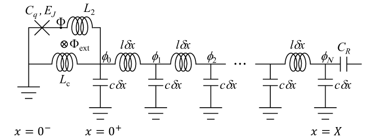
Figure 1: Schematic diagram of the qubit-TLR system, with the TLR modeled as a series of LC elements. After setting up the equations with a finite length $\delta x$, we will take the limit $\delta x\to 0$. The TLR is a quarter-wavelength resonator, terminated to ground at one end and with a (near-zero-capacitance) capacitor at the other end. The qubit is modeled as a loop with a single Josephson junction, in addition to linear inductances. The loop is threaded by an externally applied flux $\Phi_{\rm ext}$. The qubit-TLR coupling arises from the shared inductance $L_{c}$. The $x$ values at the bottom show the correspondence with the original circuit and mathematical model.

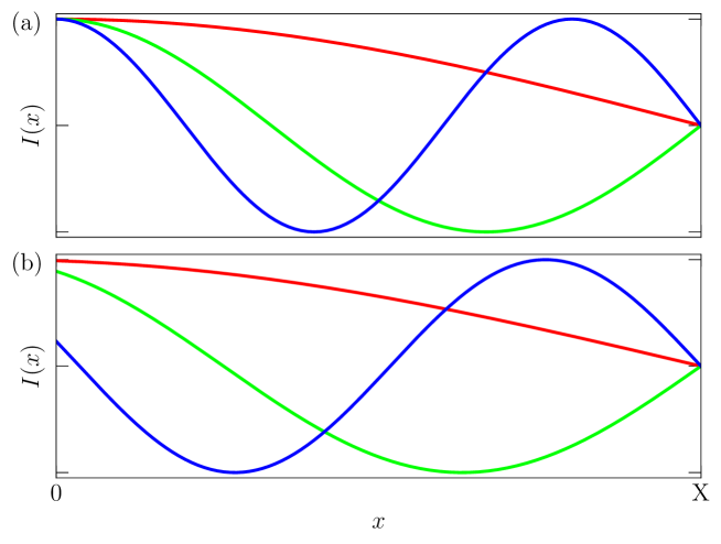
Figure 2: Electric current profiles $I(x)$ of the lowest three normal modes of the quarter-wavelength TLR in the absence of coupling to the qubit (a) and in the case of coupling to the qubit (b). Note that, apart from the profile of each function as a function of $x$, the maximum amplitudes in the figure do not have any physical significance, e.g. they should not be compared to each other. The presence of the qubit (at $x=0$) suppresses the current amplitude at the location of the qubit. The suppression effect becomes increasingly strong with increasing mode frequency, with $I(0)\to 0$ in the limit of infinitely high mode frequency. The amplitude suppression is exaggerated in this figure for clarity.

We consider the circuit shown in Fig. 1. Compared to the experimental circuit used in Ref. Ao , we make the standard simplification where we keep only one Josephson junction in the theoretical treatment. This one junction is sufficient to provide the anharmonicity needed to create a qubit. Two other (large) junctions in the qubit loop are replaced by a single inductance. The coupling junction that is shared by the qubit loop and the resonator is also replaced by a coupling inductance. As shown in Ref. Yoshihara2022 , these approximations can provide a rather accurate theoretical treatment of circuit-QED systems even in the deep-strong-coupling regime. To maximize the coupling between the qubit and TLR, the TLR is shorted to the ground at the end where the qubit is located. In this case, all TLR normal modes have maximum current amplitudes at the location of the qubit, as illustrated by the electric current profiles in Fig. 2(a). The other end of the TLR is terminated by a capacitor. We replace the spatially extended TLR by a long series of small inductances and capacitors, as is standard in the literature. Each inductance-capacitor pair corresponds to a segment of length $\delta x$ of the TLR. At some point in our derivations below, we take the limit in which the inductance-capacitance series is replaced by an infinite series of infinitesimally small elements, corresponding to the infinitesimal length $dx$.

We follow the standard technique for calculating the quantum mechanical Hamiltonian for superconducting circuits Devoret ; Vool . From the circuit diagram shown in Fig. 1, we can construct the Lagrangian:

$$\mathcal{L} = \frac{1}{2}C_{q}\dot{\Phi}^{2}-U_{q}(\Phi,\Phi_{\rm ext})+\sum_{j=0}^{N}\frac{1}{2}c\delta x\dot{\phi}_{j}^{2}-\sum_{j=0}^{N-1}\frac{1}{2l\delta x}\left(\phi_{j}-\phi_{j+1}\right)^{2}$$ (1)

$$\hskip 170.71652pt-\frac{1}{2L_{c}}\phi_{0}^{2}-\frac{1}{2L_{2}}\left(\Phi-\phi_{0}\right)^{2}+\frac{1}{2}C_{R}\dot{\phi}_{N}^{2}.$$

The flux (or phase) variable $\Phi$ represents the qubit variable that introduces the nonlinearity in the circuit via the effective Josephson potential $U_{\rm{q}}(\Phi,\Phi_{\rm ext})=-E_{J}\cos\left\{{2\pi(\Phi-\Phi_{\rm ext})/\Phi_{0}}\right\}$. The coefficient $E_{J}=I_{c}\Phi_{0}/(2\pi)$ is the Josephson energy of the junction, $I_{c}$ is the critical current, and $\Phi_{0}=h/(2e)$ is the superconducting flux quantum. The variables $\phi_{j}$ are the phase variables at the nodes $j$ ($j=0,1,2,...,N$) along the TLR. The capacitance $C_{q}$ is the junction capacitance. The parameters $c$ and $l$ are, respectively, the capacitance and the inductance per unit length of the TLR, such that the capacitances and inductances of the elements shown in Fig. 1 are given by $c\delta x$ and $l\delta x$.

Using the Legendre transformation,

$$Q = \frac{\partial\mathcal{L}}{\partial\dot{\Phi}}=C_{q}\dot{\Phi}$$ (2)

$$\delta q_{j} = \frac{\partial\mathcal{L}}{\partial\dot{\phi}_{j}}=c\delta x\dot{\phi}_{j},\ 0\leq j<N$$ (3)

$$\delta q_{N} = \frac{\partial\mathcal{L}}{\partial\dot{\phi}_{N}}=(C_{R}+c\delta x)\dot{\phi}_{N},$$ (4)

we obtain the Hamiltonian:

$$\mathcal{H} = \frac{1}{2C_{q}}Q^{2}+U_{q}(\Phi,\Phi_{\rm ext})+\sum_{j=0}^{N-1}\left(\frac{1}{2c\delta x}\delta q_{j}^{2}+\frac{1}{2l\delta x}\left(\phi_{j}-\phi_{j+1}\right)^{2}\right)$$ (5)

$$\hskip 142.26378pt+\frac{1}{2L_{c}}\phi_{0}^{2}+\frac{1}{2L_{2}}\left(\Phi-\phi_{0}\right)^{2}+\frac{1}{2(C_{R}+c\delta x)}\delta q_{N}^{2}.$$

As is common in the theoretical treatment of superconducting circuits, the main changes that occur when going from the Lagrangian to the Hamiltonian are: (1) the phase variable derivatives are replaced by charge variables, (2) capacitances move from numerators to denominators, and (3) the signs of the potential energy terms are reversed. The smallness of $\delta x$ add the following feature in our case: the new variables $\delta q$ are proportional to $\delta x$. Hence, the term $\delta q_{j}^{2}/(2c\delta x)$ is also proportional to $\delta x$. Similarly, since the difference $\phi_{j}-\phi_{j+1}$ is equal to the spatial derivative of the phase variable multiplied by $\delta x$, the term $\left(\phi_{j}-\phi_{j+1}\right)^{2}/(2l\delta x)$ is proportional to $\delta x$. These properties are to be expected and allow a smooth transition from this discrete description to the continuous description that we shall introduce shortly.

It might be worth pointing out another interesting property of the Hamiltonian: although $L_{c}$ is the mutual inductance between the qubit and the TLR, it is $L_{2}$ that appears in the Lagrangian and Hamiltonian terms that combine the qubit and TLR variables, i.e. the variables $\Phi$ and $\phi_{0}$. Furthermore, $L_{2}$ appears in the denominator, whereas we expect the mutual inductance to appear in the numerator in the effective coupling term, which should be equal to the mutual inductance times the product of the qubit and TLR currents. This situation might seem paradoxical. However, it is simply a matter of deceptive appearance in the intermediate steps of the derivation. For example, a somewhat similar situation occurs in Ref. Yoshihara2022 . In that case a Y-$\Delta$ transformation produces a coupling term that has the coupling inductance $L_{c}$ in the numerator, as intuitively expected. It is less obvious how a similar transformation could give rise to logical-looking coupling term in the present case. We will show in Appendix B how a careful analysis of the Hamiltonian produces logical results. For the time being, we just point out that if we set $L_{c}=0$, we find that we must have $\phi_{0}=0$ to avoid a divergence in the $\phi_{0}^{2}/(2L_{c})$ term, which in turn causes the term $\Phi\phi_{0}/L_{2}$ to vanish. Hence we indirectly obtain the expected result that the value $L_{c}=0$ corresponds to decoupled subsystems.

III Equations of motion and boundary conditions

From the Hamiltonian, we can derive the equations of motion for the dynamical variables straightforwardly:

$$\dot{Q} = -\frac{\partial\mathcal{H}}{\partial\Phi}=-\frac{dU_{q}(\Phi,\Phi_{\rm ext})}{d\Phi}-\frac{\Phi-\phi_{0}}{L_{2}}$$ (6)

$$\dot{\Phi} = \frac{\partial\mathcal{H}}{\partial Q}=\frac{Q}{C_{q}}$$ (7)

$$\dot{\delta q}_{j} = -\frac{\partial\mathcal{H}}{\partial\phi_{j}}=\left\{\begin{array}[]{lll}\frac{\phi_{1}-\phi_{0}}{l\delta x}-\frac{\phi_{0}}{L_{c}}+\frac{\Phi-\phi_{0}}{L_{2}}&&j=0,\\ \frac{\phi_{j+1}-2\phi_{j}+\phi_{j-1}}{l\delta x}&&1\leq j<N,\\ \frac{-\phi_{N}+\phi_{N-1}}{l\delta x}&&j=N,\end{array}\right.$$ (11)

$$\dot{\phi}_{j} = \frac{\partial\mathcal{H}}{\partial\delta q_{j}}=\left\{\begin{array}[]{lll}\frac{\delta q_{j}}{c\delta x}&&0\leq j<N,\\ \frac{\delta q_{N}}{C_{R}+c\delta x}&&j=N.\end{array}\right.$$ (14)

It is convenient for the analysis below to turn the first-order equations of motion into second-order equations of motion for the phase variables

$$\ddot{\Phi} = -\frac{1}{C_{q}}\frac{dU_{q}(\Phi,\Phi_{\rm ext})}{d\Phi}-\frac{\Phi-\phi_{0}}{C_{q}L_{2}}$$ (15)

$$\ddot{\phi}_{j} = \left\{\begin{array}[]{lll}\frac{\phi_{1}-\phi_{0}}{cl\delta x^{2}}-\frac{\phi_{0}}{c\delta xL_{c}}+\frac{\Phi-\phi_{0}}{c\delta xL_{2}}&&j=0,\\ \frac{\phi_{j+1}-2\phi_{j}+\phi_{j-1}}{cl\delta x^{2}}&&1\leq j<N,\\ \frac{-\phi_{N}+\phi_{N-1}}{l\delta x(C_{R}+c\delta x)}&&j=N.\end{array}\right.$$ (19)

We now take the limit in which $\delta x$ becomes the infinitesimal $dx$, and we obtain the continuous version of Eqs. (15,19):

$$\ddot{\Phi} = -\frac{1}{C_{q}}\frac{dU_{q}(\Phi,\Phi_{\rm ext})}{d\Phi}-\frac{\Phi-\phi(x=0^{+})}{C_{q}L_{2}}$$ (20)

$$\frac{\partial^{2}\phi}{\partial t^{2}} = \left\{\begin{array}[]{lll}\left(\frac{1}{cl}\frac{\partial\phi}{\partial x}-\frac{\phi}{cL_{c}}+\frac{\Phi-\phi}{cL_{2}}\right)\delta(x)&&x=0,\\ \frac{1}{cl}\frac{\partial^{2}\phi}{\partial x^{2}}&&x>0.\end{array}\right.$$ (23)

In Eq. (23), $\delta(x)$ is the Dirac delta function, which is the natural limit for the factor $1/\delta x$, since the Dirac delta function can be thought of as an extremely narrow step-function peak whose height is the inverse of its width. From a different point of view, the role of the $j=0$ or $x=0^{+}$ point is to set the effective boundary condition for the variable in the TLR just to the right of the qubit in Fig. 1. The Dirac delta function naturally plays this role, as we shall see shortly.

Since the TLR is connected to the ground at $x=0$ (to the left of the qubit), the boundary condition there is

$$\phi(x)\Big{|}_{x=0^{-}} = 0.$$ (24)

If the TLR is well isolated from the environment on the right-hand side of Fig. 1, the capacitance $C_{R}$ will be small. For purposes of this argument, we can take the limit $C_{R}\to 0$. Considering that $(-\phi_{N}+\phi_{N-1})/\delta x=-\partial\phi/\partial x$, we find that to avoid a divergence in the last line of Eq. (19) the boundary condition at $x=X$ (where $X$ is the length of the TLR) must be

$$\frac{\partial\phi}{\partial x}\Bigg{|}_{x=X} = 0.$$ (25)

In physical terms, this boundary condition means that the current at $x=X$ is equal to zero, which is needed to prevent the accumulation of an infinite charge density at that point.

By integrating Eq. (23) from $x=0^{-}$ to $x=0^{+}$ to evaluate $\phi(x=0^{+})$, the equations of motion can be rewritten in the simpler form:

$$\ddot{\Phi} = -\frac{1}{C_{q}}\frac{dU_{q}(\Phi,\Phi_{\rm ext})}{d\Phi}-\frac{\Phi-\phi(x=0)}{C_{q}L_{2}}$$ (26)

$$\frac{\partial^{2}\phi}{\partial t^{2}} = \frac{1}{cl}\frac{\partial^{2}\phi}{\partial x^{2}},$$ (27)

with modified boundary conditions:

$$\left(\frac{1}{cl}\frac{\partial\phi}{\partial x}-\frac{\phi}{cL_{c}}+\frac{\Phi-\phi}{cL_{2}}\right)\Bigg{|}_{x=0} = 0$$ (28)

$$\frac{\partial\phi}{\partial x}\Bigg{|}_{x=X} = 0.$$ (29)

IV TLR modes and high-frequency decoupling

We now calculate the frequencies and electric current profiles of the normal modes in the TLR. First, we note that the presence of $\Phi$ in the boundary condition in Eq. (28) means that in principle the equations for $\phi$ cannot be solved without knowledge of $\Phi$. We can however, eliminate $\Phi$ from the equations for $\phi$ under the approximation that $\Phi$ exhibits only small dynamical deviations away from its mean value $\overline{\Phi}$, which is a reasonable assumption for the low-energy states of the system. A more detailed derivation on this point is given in Appendix A. If we define the new variable

$$\tilde{\phi}(x)=\phi(x)-\frac{L_{c2}}{L_{2}}\overline{\Phi},$$ (30)

where $L_{c2}=L_{c}L_{2}/(L_{c}+L_{2})$, we obtain $\Phi$-independent equations for $\tilde{\phi}$. The equations are, to a good approximation, given by

$$\frac{\partial^{2}\tilde{\phi}}{\partial t^{2}} = \frac{1}{cl}\frac{\partial^{2}\tilde{\phi}}{\partial x^{2}}$$ (31)

$$\left(\frac{1}{cl}\frac{\partial\tilde{\phi}}{\partial x}-\frac{\tilde{\phi}}{cL_{c2}}\right)\Bigg{|}_{x=0} = 0$$ (32)

$$\frac{\partial\tilde{\phi}}{\partial x}\Bigg{|}_{x=X} = 0.$$ (33)

We can now determine the normal modes by solving this one-dimensional wave equation. We do so by substituting sinusoidally oscillating solutions with temporal frequency $\omega$:

$$\tilde{\phi}(x,t)=e^{-i\omega t}u(x),$$ (34)

which gives

$$-\omega^{2}u(x) = \frac{1}{cl}\frac{d^{2}u}{dx^{2}}$$ (35)

$$\left(\frac{1}{cl}\frac{du}{dx}-\frac{u}{cL_{c2}}\right)\Bigg{|}_{x=0} = 0$$ (36)

$$\frac{du}{dx}\Bigg{|}_{x=X} = 0.$$ (37)

The solution of the wave equation in Eq. (35) can be expressed as

$$u(x)=u_{c}\cos(k[x-x_{0}]),$$ (38)

where $k=\sqrt{\omega^{2}cl}$. The parameters $k$ and $x_{0}$ are parameters that are determined by the boundary conditions. It is worth noting here that, since the differential equation and boundary conditions are linear, they do not impose any conditions on $u_{c}$. As we will see below, $u_{c}$ will be governed by energy quantization. Considering the boundary condition at $x=X$, we can write $u(x)$ as

$$u(x)=u_{c}\cos(k[x-X]).$$ (39)

The boundary condition at $x=0$ now gives

$$\frac{k}{cl}\sin(kX)-\frac{1}{cL_{c2}}\cos(kX)=0,$$ (40)

and therefore

$$k\tan(kX)=\frac{l}{L_{c2}}.$$ (41)

This transcendental equation has an infinite number of solutions, i.e. there are an infinite number of $k$ values that satisfy the equation, as illustrated in Fig. 3. These solutions characterize the TLR modes. We will analyze various properties of the solutions below.

It is helpful at this point to rewrite Eq. (41) in the form

$$\omega\tan(kX)=\omega_{\rm cutoff},$$ (42)

or alternatively,

$$\omega\tan(\omega\sqrt{cl}X)=\omega_{\rm cutoff},$$ (43)

where

$$\omega_{\rm cutoff}=\frac{Z_{0}}{L_{c2}},$$ (44)

and $Z_{0}=\sqrt{l/c}$ is the impedance of the TLR, typically set to 50 $\Omega$. This expression for $\omega_{\rm cutoff}$ is the one for a low-pass filter, similarly to what was found in Ref. Malekakhlagh2017 for capacitive coupling. Similar expressions appear in Refs. Gely ; ParraRodriguez ; Shitara . The physical meaning of this expression will become clear when we discuss the high-frequency limit below.

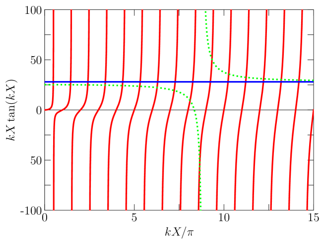
Figure 3: The function $kX\tan(kX)$, shown in red, as a function of $kX/\pi$. The horizontal blue line corresponds to $Xl/L_{c2}=28$, which corresponds to the parameters of Ref. Ao . The points of intersection between the red and blue lines correspond to solutions of Eq. (41). For the low-frequency modes, i.e. at small values of $kX$, these intersection points are close to half-integer values of $kX/\pi$. For the high-frequency modes, as we go to increasingly large values of $kX$, the intersection points become increasingly close to integer values of $kX/\pi$. The green dotted line replaces the blue line in the more precise calculation presented in Appendix A, with the parameters $\omega_{q}\sqrt{cl}X/\pi=8.8$ and $L_{c}L_{q}/[(L_{c}+L_{2})(L_{q}+L_{2})]=0.1$. The intersection points between the red and green lines give the solutions to Eq. (103).

IV.1 Low-frequency modes

For the low-frequency modes with $\omega\ll\omega_{\rm cutoff}$, the solutions of Eq. (42) must have $\tan(kX)\gg 1$, which implies that $kX$ is slightly smaller than $n\pi+\pi/2$ with $n$ being an integer. We therefore define the small variable $\widetilde{kX}=n\pi+\pi/2-kX$. By rearranging Eq. (41) and making use of the first-order approximation that $\cot(n\pi+\pi/2-\delta)\approx\delta$ for $\delta\ll 1$, we obtain

$$n\pi+\frac{\pi}{2}-\widetilde{kX} = \frac{Xl}{L_{c2}}\cot(n\pi+\frac{\pi}{2}-\widetilde{kX})$$ (45)

$$\approx \frac{Xl}{L_{c2}}\widetilde{kX}.$$

As a result,

$$\widetilde{kX}\approx\frac{n\pi+\frac{\pi}{2}}{1+Xl/L_{c2}}.$$ (46)

Taking into consideration the fact that $Xl/L_{c2}\gg 1$ (which is required for the validity of the condition $\omega\ll\omega_{\rm cutoff}$), we obtain the approximation

$$kX\approx n\pi+\frac{\pi}{2}-\frac{\left(n\pi+\frac{\pi}{2}\right)}{1+Xl/L_{c2}}\approx\left(n\pi+\frac{\pi}{2}\right)\times\left(1-\frac{L_{c2}}{Xl}\right),$$ (47)

starting at $n=0$ for the fundamental mode. From now on, we will refer to the value of $k$ that corresponds to an integer $n$ as $k_{n}$, and we refer to the corresponding frequency as $\omega_{n}$.

IV.2 Fundamental mode

Using the above expression for $k_{n}X$, we find the (zeroth-order) approximate expression for the fundamental mode frequency

$$\omega_{0}=\frac{\pi}{2X\sqrt{cl}}=\frac{\pi Z_{0}}{2Xl}=\frac{\pi}{2XZ_{0}c},$$ (48)

as should be expected for a quarter wavelength resonator. It is worth noting that with this expression for $\omega_{0}$, we find that $Xl/L_{c2}=\pi\omega_{\rm cutoff}/(2\omega_{0})$, and Eq. (41) can be rewritten as

$$k_{n}X\tan(k_{n}X)=\frac{\pi\omega_{\rm cutoff}}{2\omega_{0}}.$$ (49)

It is also worth noting that the factor $(1-L_{c2}/Xl)$ in Eq. (47) is approximately equal to $Xl/(Xl+L_{c2})$. Using the expression $\omega_{0}=\pi Z_{0}/(2Xl)$, the small deviation of the factor $Xl/(Xl+L_{c2})$ from unity can be understood in terms of the inductance $L_{c2}$ increasing the total inductance of the TLR from $Xl$ to $Xl+L_{c2}$.

IV.3 High-frequency modes

For the high-frequency modes with $\omega\gg\omega_{\rm cutoff}$, the solutions of Eq. (41) must have $\tan(k_{n}X)\ll 1$, which means that $k_{n}X$ must be slightly larger than $n\pi$, with $n$ being an integer. We therefore define $\widetilde{k_{n}X}=k_{n}X-n\pi$, which gives

$$(n\pi+\widetilde{k_{n}X})\tan(n\pi+\widetilde{k_{n}X})=\frac{Xl}{L_{c2}}.$$ (50)

Using the approximation that $\tan(n\pi+\delta)\approx\delta$ for $\delta\ll 1$, we obtain the first-order approximation in $\omega_{\rm cutoff}/\omega$

$$\widetilde{k_{n}X}=\frac{Xl}{n\pi L_{c2}}.$$ (51)

This formula in turn gives the approximate expression for $k_{n}X$:

$$k_{n}X\approx n\pi+\frac{Xl}{n\pi L_{c2}}.$$ (52)

Note that in the limit $n\rightarrow\infty$, we obtain $k_{n}X=n\pi$, and the boundary condition at $x=0$ effectively becomes $du/dx=0$, which is the appropriate boundary condition if the TLR were terminated with capacitors at both ends, i.e. the connection to the ground is effectively cut and no (high-frequency) current flows at the point where the qubit is located. The low-pass-filter behavior now becomes clear. In fact, this behavior is perhaps more intuitive for the circuit with inductive coupling compared to the case of capacitive coupling studied in Ref. Malekakhlagh2017 . The intuitive picture of an inductance is as a circuit element that resists changes in current. Put differently, the impedance of an inductance $L$ at frequency $\omega$ is given by $i\omega L$. The time derivative of an ac current in the inductance is given by the product of the oscillation amplitude and the frequency. Increasing the frequency leads to stronger resistance by the inductance, which can be alleviated by suppressing the oscillation amplitude. In the limit of infinite frequency, the current at the location of the low-pass filter must be suppressed to zero to avoid an infinite resistance from the inductance.

In addition to $\omega_{\rm cutoff}$, we can also define the parameter $n_{\rm cutoff}$ as an estimate for the number of TLR modes whose coupling to the qubit is not significantly suppressed:

$$n_{\rm cutoff}=\frac{\omega_{\rm cutoff}}{\omega_{0}}=\frac{2Xl}{\pi L_{c2}}$$ (53)

The actual number of modes below the cutoff frequency is $n_{\rm cutoff}/2$. The factor of 2 in the denominator arises because the fundamental mode ($n=0$) has $k_{0}X=\pi/2$ while the high-frequency modes have $k_{n}X\approx n\pi$. Another way to look at the factor of 2 is to note that the normal mode frequencies of a quarter-wavelength resonator are odd multiples of the fundamental mode frequency, and the even multiples are missing. It should be emphasized, however, that this factor does not have too much significance, because the current suppression with increasing mode frequency is a gradual process and not a sharp cutoff.

IV.4 Coupling strengths between qubit and TLR normal modes

Now that we have determined the frequencies and current profiles of the normal modes in the TLR, we can calculate their quantum properties and determine how they interact with the qubit. From the form of the Hamiltonian, we can see that the energy is proportional to $u_{c}^{2}$:

$$E=\frac{Xk_{n}^{2}u_{c}^{2}}{2l},$$ (54)

provided that $n\gg 1$. In the ground state of any of the modes, the energy should be $E=\hbar\omega_{n}/2$, which is the ground-state energy of a harmonic oscillator. Equating these two formulae for the energy gives the formula for the zero-point (root-mean-square) fluctuations in the mode variable:

$$u_{c,\rm rms}=\sqrt{\frac{\hbar}{Xc\omega_{n}}}.$$ (55)

These fluctuations give the zero-point current fluctuations at $x=0$:

$$\frac{1}{l}\left|\frac{\partial u}{\partial x}\right|_{x=0,\rm rms} = \sqrt{\frac{\hbar}{Xc\omega_{n}}}\frac{k_{n}\sin(k_{n}X)}{l}$$ (56)

$$= \sqrt{\frac{\hbar k_{n}^{2}}{Xl^{2}c\omega_{n}}}\times\sqrt{\frac{\tan^{2}(k_{n}X)}{1+\tan^{2}(k_{n}X)}}$$

$$= \sqrt{\frac{\hbar\omega_{n}}{Xl}}\times\frac{1}{\sqrt{1+\left(\frac{\omega_{n}}{\omega_{\rm cutoff}}\right)^{2}}}$$

$$= \frac{1}{Xl}\sqrt{\frac{\hbar\pi Z_{0}}{2}}\times\sqrt{\frac{\omega_{n}/\omega_{0}}{1+\left(\frac{\omega_{n}}{\omega_{\rm cutoff}}\right)^{2}}}.$$

This expression can be substituted in the formula

$$\hbar g_{n}=L_{c}\times I_{\rm qubit}\times\frac{1}{l}\left|\frac{\partial u}{\partial x}\right|_{x=x_{\rm qubit},\rm rms}$$ (57)

to obtain the coupling strength $g_{n}$ as a function of mode frequency $\omega_{n}$. Here $g_{n}$ is the parameter that enters in the quantum Rabi model (QRM) Hamiltonian

$$\mathcal{H}_{QRM}=-\frac{\Delta_{0}}{2}\sigma_{x}-\frac{\epsilon}{2}\sigma_{z}+\sum_{n=0}^{\infty}\left\{\hbar\omega_{n}\left(a_{n}^{\dagger}a_{n}+\frac{1}{2}\right)+\hbar g_{n}\left(a_{n}+a_{n}^{\dagger}\right)\right\},$$ (58)

where $\Delta_{0}$ is the bare qubit gap, i.e. not including renormalization by the Lamb shift, $\epsilon$ is the qubit bias, $\sigma_{x}$ and $\sigma_{z}$ are qubit Pauli operators, and $a_{n}$ and $a_{n}^{\dagger}$ are, respectively, the annihilation and creation operators for mode $n$. The coupling strength $g_{n}$ grows as $\sqrt{\omega_{n}}$ for $\omega\ll\omega_{\rm cutoff}$ and decreases as $1/\sqrt{\omega_{n}}$ for $\omega\gg\omega_{\rm cutoff}$, as found in several recent studies.

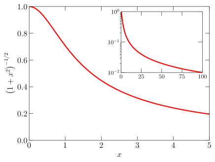
Figure 4: The factor $1/\sqrt{(1+x^{2})}$, which describes the suppression of the coupling strength with increasing $x=\omega/\omega_{\rm cutoff}$. Here the variable $x$ represents the ratio $\omega/\omega_{\rm cutoff}$. The inset shows the same function over a broader range of $x$ values, with the $y$ axis plotted using a logarithmic scale.

IV.5 Dependence of coupling strength on mode frequency and coupling inductance

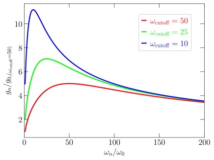
Figure 5: Coupling strength $g_{n}$ as a function of mode frequency $\omega_{n}$ for three different values of the coupling inductance $L_{c}$. The different $L_{c}$ values are identified by the resulting $\omega_{\rm cutoff}$ values. Here it is assumed that all system parameters other than $L_{c}$ are kept fixed and $L_{2}\gg L_{c}$, such that $\omega_{\rm cutoff}\propto 1/L_{c}$. The mode frequency $\omega_{n}$ is measured relative to the fundamental mode frequency $\omega_{0}$. The coupling strength $g_{n}$ is measured relative to $g_{0}$ for the $L_{c}$ value that gives $\omega_{\rm cutoff}=50$.

We now consider the dependence of $g_{n}$ on $\omega_{n}$. Since the coupling between the qubit and the TLR arises from the shared coupling inductance $L_{c}$, it is interesting to also ask how $g_{n}$ depends on $L_{c}$. There is a factor $L_{c}$ that appears explicitly in Eq. (57). Both qubit and TLR currents also depend on $L_{c}$ in principle, because the same inductance that mediates the coupling can be seen as part of the qubit loop and part of the TLR circuit. For example, following Ref. Yoshihara2022 , the qubit’s persistent current is given by

$$I_{\rm qubit}\sim\frac{\Phi_{0}}{\pi(L_{c}+L_{2})}.$$ (59)

In other words, the flux qubit’s persistent current $I_{\rm qubit}$ depends on $L_{c}$. However, if we consider the weak-coupling regime with $L_{c}\ll L_{2}$, and $L_{c}\ll Xl$, the qubit and low-frequency mode currents are independent of $L_{c}$ to lowest order. This approximation gives for the low-frequency modes

$$\hbar g_{n} \sim L_{c}\times I_{\rm qubit}\times\frac{1}{Xl}\sqrt{\frac{\hbar\pi Z_{0}}{2}}\times\sqrt{\frac{\omega_{n}}{\omega_{0}}}\left(1-\frac{1}{2}\left(\frac{\omega_{n}}{\omega_{\rm cutoff}}\right)^{2}\right)$$ (60)

$$= L_{c}\times I_{\rm qubit}\times\sqrt{\frac{\hbar\omega_{n}}{Xl}}\times\left(1-\frac{1}{2}\left(\frac{\omega_{n}}{\omega_{\rm cutoff}}\right)^{2}\right).$$

In other words, $g_{n}\propto\sqrt{\omega_{n}}$, with relative corrections on the order of $(\omega_{n}/\omega_{\rm cutoff})^{2}$. This result is consistent with the low-frequency behavior obtained in previous studies. Additionally, we note that $g_{n}\propto L_{c}$. This result is intuitively to be expected, considering that $L_{c}$ is the mutual coupling inductance. This behaviour is illustrated in Fig. 5.

For the high-frequency modes

$$\frac{1}{l}\left|\frac{\partial u}{\partial x}\right|_{x=0,\rm rms} \sim \frac{1}{Xl}\sqrt{\frac{\hbar\pi Z_{0}}{2}}\times\sqrt{\frac{\omega_{\rm cutoff}^{2}}{\omega_{n}\omega_{0}}}$$ (61)

$$= \frac{1}{XlL_{c}}\sqrt{\frac{\hbar\pi Z_{0}^{3}}{2\omega_{n}\omega_{0}}}$$

$$= \frac{1}{L_{c}}\sqrt{\frac{\hbar Z_{0}^{2}}{Xl\omega_{n}}},$$

which gives

$$\hbar g_{n}\sim I_{\rm qubit}\sqrt{\frac{\hbar Z_{0}^{2}}{Xl\omega_{n}}}=I_{\rm qubit}\sqrt{\frac{2\hbar Z_{0}\omega_{0}}{\pi\omega_{n}}}.$$ (62)

In agreement with past studies, $g_{n}\propto 1/\sqrt{\omega_{n}}$. Furthermore, Eq. (62) indicates that the coupling strength is independent of the mutual inductance $L_{c}$ for the high-frequency modes, as can be seen in Fig. 5. This result is quite interesting. It means that we cannot increase the coupling strength to high frequency modes by increasing the qubit-TLR mutual inductance. Instead, treating $Z_{0}$ and $\omega_{n}$ as constants, the two possible approaches to increase $g_{n}$ are either increasing $I_{\rm qubit}$ or reducing the total TLR inductance $Xl$.

Note that in this section we assumed that $L_{c}$ is small compared to other inductances in the circuit in order to be able to derive simple expressions. Taking large $L_{c}$ would significantly modify the behavior of the dynamical variables, which can lead to significant deviations from the approximate expressions that we derived. This situation could require numerical analysis of the equations of motion etc. We will not perform any such analysis in this paper.

IV.6 Modified frequency pattern for the low-frequency modes

In the absence of the qubit, the mode frequencies of a quarter-wavelength TLR follow the pattern: $\omega_{1}/\omega_{0}=3$, $\omega_{2}/\omega_{0}=5$, …, i.e. $\omega_{n}/\omega_{0}=(2n+1)$. We now consider the correction to this pattern induced by the finiteness of $L_{c2}/Xl$. The motivation to look for such deviations is that a modified pattern could serve as an experimental test for the theory and a means to infer system parameters from measured spectra.

As can be seen from Eq. (47), the pattern $\omega_{n}/\omega_{0}=(2n+1)$ for the low-frequency modes is preserved at the lowest order considered in Sec. IVA. To calculate the desired corrections, we must include the next order in the expansion of the cotangent function: $\cot(n\pi+\pi/2-\delta)\approx\delta+\delta^{3}/3$, i.e.

$$n\pi+\frac{\pi}{2}-\widetilde{k_{n}X} = \frac{Xl}{L_{c2}}\cot(n\pi+\frac{\pi}{2}-\widetilde{k_{n}X})$$ (63)

$$\approx \frac{Xl}{L_{c2}}\left(\widetilde{k_{n}X}+\frac{(\widetilde{k_{n}X})^{3}}{3}\right).$$

This equation can be rearranged into the form

$$\widetilde{k_{n}X}\approx\frac{1}{1+Xl/L_{c2}}\left(n\pi+\frac{\pi}{2}-\frac{Xl}{L_{c2}}\frac{(\widetilde{k_{n}X})^{3}}{3}\right),$$ (64)

We now take the lowest-order approximation for $\widetilde{k_{n}X}$, i.e. $\widetilde{k_{n}X}\approx(n\pi+\pi/2)/(1+Xl/L_{c2})$, and we substitute it in the cubic term on the right-hand side of Eq. (77) to obtain

$$\widetilde{k_{n}X}\approx\frac{n\pi+\frac{\pi}{2}}{1+Xl/L_{c2}}-\frac{1}{3}\frac{Xl/L_{c2}}{(1+Xl/L_{c2})^{4}}\left(n\pi+\frac{\pi}{2}\right)^{3},$$ (65)

and therefore

$$k_{n}X\approx\left(n\pi+\frac{\pi}{2}\right)\left[1-\frac{1}{1+Xl/L_{c2}}+\frac{1}{3}\frac{Xl/L_{c2}}{(1+Xl/L_{c2})^{4}}\left(n\pi+\frac{\pi}{2}\right)^{2}\right].$$ (66)

This expression then leads to the approximate relation

$$\frac{\omega_{n}}{\omega_{0}}=\frac{k_{n}}{k_{0}} \approx (2n+1)\times\left[1+\frac{1}{3}\frac{\left(n\pi+\frac{\pi}{2}\right)^{2}}{(Xl/L_{c2})^{3}}-\frac{1}{3}\frac{\left(\frac{\pi}{2}\right)^{2}}{(Xl/L_{c2})^{3}}\right]$$ (67)

$$= (2n+1)\times\left[1+\frac{\pi^{2}}{3}\left(\frac{L_{c2}}{Xl}\right)^{3}\left(n^{2}+n\right)\right]$$

$$= (2n+1)\times\left[1+\frac{8\left(n^{2}+n\right)}{3\pi n_{\rm cutoff}^{3}}\right].$$

For the lowest three modes, we find that $\omega_{1}/\omega_{0}\approx 3+16/(\pi n_{\rm cutoff}^{3})$ and $\omega_{2}/\omega_{0}\approx 5+80/(\pi n_{\rm cutoff}^{3})$. In Ref. Ao , $n_{\rm cutoff}=13.2$, which gives $\omega_{1}/\omega_{0}-3\approx 0.002$ and $\omega_{2}/\omega_{0}-5\approx 0.01$. In other words, for $\omega_{0}/(2\pi)\approx 2.5$ GHz we obtain $(\omega_{1}-3\omega_{0})/(2\pi)\approx 5$ MHz and $(\omega_{2}-5\omega_{0})/(2\pi)\approx 25$ MHz. Since the measurement accuracy for resonance frequencies in spectroscopy measurements is typically well below 1 MHz, a deviation of 5 MHz should be measurable experimentally.

In the context to calculating small variations in $\omega_{n}/\omega_{0}$, we consider the effect of having a finite $C_{R}$ on the mode frequencies. For this calculation, we ignore the presence of the qubit and focus on the effect of the finite $C_{R}$. The wave equation for $\phi$ is still given by Eq. (27), and its solution can still be expressed as

$$\phi(x,t)=u_{c}e^{-i\omega t}\cos(k[x-x_{0}]),$$ (68)

with $\omega=k/\sqrt{cl}$. In the absence of the qubit, the boundary condition at $x=0$ is $\phi(x)|_{x=0}=0$, which allows us to express $\phi(x,t)$ as

$$\phi(x,t)=u_{c}e^{-i\omega t}\sin(kx).$$ (69)

The last line of Eq. (19), along with the $e^{-i\omega t}$ time dependence of $\phi(x,t)$, now gives the boundary condition:

$$\left(-\omega^{2}\phi+\frac{1}{lC_{R}}\frac{d\phi}{dx}\right)\Bigg{|}_{x=X}=0.$$ (70)

Substituting Eq. (69) into Eq. (70) gives the transcendental equation

$$k\tan(kX)=\frac{c}{C_{R}}.$$ (71)

This equation has exactly the same form as Eq. (41), but with $c/C_{R}$ instead of $l/L_{c2}$ on the right-hand side of the equation. Considering the case $C_{R}/(Xc)\ll 1$, we can use the same derivation as the one used earlier in this subsection and obtain

$$\frac{\omega_{n}}{\omega_{0}}\approx(2n+1)\times\left[1+\frac{\pi^{2}}{3}\left(\frac{C_{R}}{Xc}\right)^{3}\left(n^{2}+n\right)\right].$$ (72)

The effect of a finite $C_{R}$ is therefore to modify the ratios $\omega_{n}/\omega_{0}$ in the same way that the coupling to the qubit modifies the frequency ratios. Depending on the relationship between the two small parameters $L_{c2}/(Xl)$ and $C_{R}/(Xc)$, either one of the two mechanisms can be dominant.

The design parameters of Ref. Ao are $X=10.75$ mm, $l=437$ nH/m, $c=162$ pF/m, $L_{c}=231$ pH, $L_{2}=823$ pH and $C_{R}=3.46\times 10^{-4}$ pF. These parameters give $L_{c2}/(Xl)\sim 4\times 10^{-2}$ and $C_{R}/(Xc)\sim 2\times 10^{-4}$, which suggests that the effect of the qubit will be much larger than the effect of the finite $C_{R}$. It should be noted, however, that the coupling of the TLR to the measurement transmission line in Ref. Ao was via an additional inductance that is not included in our theoretical model. As a result, the capacitance $C_{R}$ could in principle be made very small in that experiment without affecting the coupling between the TLR and the probe signal.

Here it is worth establishing the relation between the ratio $C_{R}/(Xc)$ and the TLR’s quality factor $Q_{\rm TLR}$ (not to be confused with the charge variable $Q$ introduced in Sec. II), because $Q_{\rm TLR}$ can be measured more directly than other circuit parameters. Following Ref. Goeppl , and assuming that all dissipation in the TLR is via the $C_{R}$ capacitor, $Q_{\rm TLR}$ is given by

$$Q_{\rm TLR}=\frac{Xc}{4\omega_{0}Z_{0}C_{R}^{2}}=\frac{1}{4\omega_{0}Z_{0}Xc}\left(\frac{Xc}{C_{R}}\right)^{2}.$$ (73)

Using the last formula for $\omega_{0}$ in Eq. (48), we find that $4\omega_{0}Z_{0}Xc=2\pi$. As a result, we obtain the formula

$$Q_{\rm TLR}=\frac{1}{2\pi}\left(\frac{Xc}{C_{R}}\right)^{2},$$ (74)

or, in other words,

$$\frac{C_{R}}{Xc}=\frac{1}{\sqrt{2\pi Q_{\rm TLR}}}.$$ (75)

If, for example, we take the relatively low quality factor $Q_{\rm TLR}=10^{3}$, we obtain the relatively high estimate $C_{R}/(Xc)=0.013$, which is still significantly lower than the value $L_{c2}/(Xl)=0.048$ for the circuit of Ref. Ao . Since these small factors are raised to the third power in the formula for $\omega_{n}/\omega_{0}$, the effect of the qubit should be more than an order of magnitude larger than the effect of the finite $C_{R}$ in a realistic setup.

Finally, we investigate the effect of using Eq. (103) when we analyze the mode frequency pattern. First, we ignore the third-order effect in expanding the $\tan$ function that we analyzed earlier in this subsection. With $\gamma=L_{c}L_{q}/(L_{c}+L_{2})(L_{q}+L_{2})$ and $\eta_{n}=[(n\pi+\frac{\pi}{2})^{2}/(X^{2}cl\omega_{q}^{2})]-1=[(2n+1)^{2}\omega_{0}^{2}/\omega_{q}^{2}]-1$, Eq. (45) is replaced by

$$n\pi+\frac{\pi}{2}-\widetilde{kX} \approx \frac{Xl}{L_{c2}}\widetilde{kX}\times\left(1+\frac{\gamma}{\frac{(n\pi+\frac{\pi}{2}-\widetilde{kX})^{2}}{X^{2}cl\omega_{q}^{2}}-1}\right)$$ (76)

$$\approx \frac{Xl}{L_{c2}}\widetilde{kX}\times\left(1+\gamma\left[\frac{1}{\eta_{n}}+\frac{4(2n+1)\omega_{0}^{2}\widetilde{kX}}{\pi\omega_{q}^{2}\eta_{n}^{2}}\right]\right).$$

This equation can be rearranged into the form

$$\widetilde{k_{n}X}\approx\frac{1}{1+\frac{Xl}{L_{c2}}\left(1+\frac{\gamma}{\eta_{n}}\right)}\left(n\pi+\frac{\pi}{2}-\frac{4(2n+1)\omega_{0}^{2}Xl\gamma}{\pi\omega_{q}^{2}\eta_{n}^{2}L_{c2}}(\widetilde{k_{n}X})^{2}\right),$$ (77)

We now take the approximation $\widetilde{k_{n}X}\approx(n\pi+\pi/2)/(1+Xl[1+\gamma/\eta_{n}]/L_{c2})$ and obtain

$$\widetilde{k_{n}X}\approx\frac{n\pi+\frac{\pi}{2}}{1+\frac{Xl}{L_{c2}}\left(1+\frac{\gamma}{\eta_{n}}\right)}-\frac{\pi\omega_{0}^{2}Xl\gamma/(\omega_{q}^{2}\eta_{n}^{2}L_{c2})}{\left(1+\frac{Xl}{L_{c2}}\left(1+\frac{\gamma}{\eta_{n}}\right)\right)^{3}}\left(2n+1\right)^{3},$$ (78)

and therefore

$$k_{n}X\approx\left(n\pi+\frac{\pi}{2}\right)\left[1-\frac{1}{1+\frac{Xl}{L_{c2}}\left(1+\frac{\gamma}{\eta_{n}}\right)}+\frac{2\omega_{0}^{2}Xl\gamma/(\omega_{q}^{2}\eta_{n}^{2}L_{c2})}{\left(1+\frac{Xl}{L_{c2}}\left(1+\frac{\gamma}{\eta_{n}}\right)\right)^{3}}\left(2n+1\right)^{2}\right].$$ (79)

We then obtain the approximate relation

$$\frac{\omega_{n}}{\omega_{0}}=\frac{k_{n}}{k_{0}} \approx (2n+1)\times\left[1+\frac{2\omega_{0}^{2}\gamma}{\omega_{q}^{2}\eta_{n}^{2}}\frac{\left(2n+1\right)^{2}}{(Xl/L_{c2})^{2}\left(1+\frac{\gamma}{\eta_{n}}\right)^{3}}-\frac{2\omega_{0}^{2}\gamma}{\omega_{q}^{2}\eta_{n}^{2}}\frac{1}{(Xl/L_{c2})^{2}\left(1+\frac{\gamma}{\eta_{n}}\right)^{3}}\right]$$ (80)

$$= (2n+1)\times\left[1+\frac{8\omega_{0}^{2}\gamma}{\omega_{q}^{2}\eta_{n}^{2}(Xl/L_{c2})^{2}\left(1+\frac{\gamma}{\eta_{n}}\right)^{3}}\left(n^{2}+n\right)\right]$$

$$\approx (2n+1)\times\left[1+\frac{32\omega_{0}^{2}\gamma}{\pi^{2}\omega_{q}^{2}\eta_{n}^{2}n_{\rm cutoff}^{2}\left(1+\frac{\gamma}{\eta_{n}}\right)^{3}}\left(n^{2}+n\right)\right].$$

Taking $n_{\rm cutoff}=13.2$, $\gamma=0.1$ and $\omega_{q}/\omega_{0}=20$, we find $\omega_{1}/\omega_{0}-3\approx 4\times 10^{-5}$. This shift is two orders of magnitude smaller than the one calculated based on Eq. (67) and should therefore be negligible. A more important effect, however, is the fact that the factor $Xl/L_{c2}$ in Eq. (76) is now multiplied by the factor $1+\gamma/\eta_{n}$, which can be approximated as $1-\gamma$. Since Eq. (67) has the factor $(Xl/L_{c2})^{-3}$, the frequency deviations calculated from Eq. (67) will be amplified by the factor $(1-\gamma)^{-3}\approx 1.3$.

V Lamb shift

One of the important questions in the study of multimode cavity QED is the Lamb shift and its convergence as we take into account the coupling between the qubit and an increasingly large number of modes.

If the qubit frequency is small relative to the oscillator frequency, the renormalized gap, i.e. the Lamb shifted qubit frequency, is given by

$$\Delta=\Delta_{0}\exp\left\{-2\sum_{n}\left(\frac{g_{n}}{\omega_{n}}\right)^{2}\right\},$$ (81)

which is the straightforward generalization of the single-mode formula Ashhab2010

$$\Delta=\Delta_{0}\exp\left\{-2\left(\frac{g}{\omega}\right)^{2}\right\}.$$ (82)

It should be emphasized that the above formula is valid in a wide range of parameters. For example, if we think of the normalization process as occurring in steps starting at $n\to\infty$ and gradually going down to $n=0$, the above formula is valid as long as the renormalized value of $\Delta$ is smaller than $\omega_{n}$ in every step of the process. Using the formulae derived in the previous section, the formula for $\Delta$ can be expressed as

$$\Delta\approx\Delta_{0}\exp\left\{-2\left(\frac{g_{0}}{\omega_{0}}\right)^{2}\sum_{n=1,3,5,...}\frac{1}{n\left(1+\frac{n^{2}}{n_{\rm cutoff}^{2}}\right)}\right\}.$$ (83)

Using the software package Mathematica, we find that the sum in Eq. (83) is given by

$$\sum_{n=1,3,5,...}\frac{1}{n\left(1+\frac{n^{2}}{n_{\rm cutoff}^{2}}\right)}=\frac{\gamma+2\log 2}{2}+\frac{\psi(\frac{1+in_{\rm cutoff}}{2})+\psi(\frac{1-in_{\rm cutoff}}{2})}{4},$$ (84)

where $\gamma$ is Euler’s constant (approximately 0.577), and $\psi(x)$ is the digamma function. For large $n_{\rm cutoff}$, the above expression reduces to the simpler function:

$$\lim_{n_{\rm cutoff}\to\infty}\left[\sum_{n=1,3,5,...}\frac{1}{n\left(1+\frac{n^{2}}{n_{\rm cutoff}^{2}}\right)}\right] = \frac{\gamma+\log 2}{2}+\frac{\log n_{\rm cutoff}}{2}$$ (85)

$$\approx 0.635+0.5\log n_{\rm cutoff}.$$

In other words, the expression $0.635+0.5\log n_{\rm cutoff}$ provides a good approximation for the sum, as long as $n_{\rm{cutoff}}\gg 1$. This expression applies to the circuit shown in Fig. 1.

Here it is worth making a small digression and giving the related sum

$$\sum_{n=1,2,3,...}\frac{1}{n\left(1+\frac{n^{2}}{n_{\rm cutoff}^{2}}\right)}=\gamma+\frac{\psi(1+in_{\rm cutoff})+\psi(1-in_{\rm cutoff})}{2}.$$ (86)

For large $n_{\rm cutoff}$, we obtain the asymptotic behavior

$$\lim_{n_{\rm cutoff}\to\infty}\left[\sum_{n=1,2,3,...}\frac{1}{n\left(1+\frac{n^{2}}{n_{\rm cutoff}^{2}}\right)}\right]=\gamma+\log n_{\rm cutoff}.$$ (87)

This formula can be relevant to a situation in which a qubit is capacitively coupled to a half-wavelength TLR with capacitors at both ends, and the qubit is placed at one of the TLR’s ends to maximize the coupling to all modes. The differences between Eqs. (85) and (87) are intuitively logical: a slightly different constant term and a factor of 2 in the $\log n_{\rm cutoff}$ term.

The slow logarithmic dependence of the above sums means that $\Delta$ changes very slowly as a function of $n_{\rm cutoff}$. It also means that the sum remains on the order of 1 and can be treated as a constant compared to other factors that play a role in determining the Lamb shift. For example, for $n_{\rm cutoff}=100$, the sum is approximately equal to 3.

VI Conclusion

We have performed theoretical analysis of a circuit comprising a flux qubit inductively coupled to a quarter-wavelength TLR. We showed how the qubit naturally decouples from the high-frequency modes of the TLR. Our results on this point agree with past results on somewhat similar circuits. Our analysis therefore complements previous theoretical studies and adds insight into the physics of the decoupling effect. We also derived new formulae for the mode frequencies, coupling strengths and Lamb shift. By avoiding certain approximations used in previous studies, we derived more accurate results, which allow us to predict previously unknown features in the spectrum of the system. Our results can help guide future experiments to test the physics of ultrastrong and deep-strong coupling in multimode circuit QED.

Appendix A: Deriving the equations of motion for the TLR variables

In this Appendix, we provide a more detailed calculation for how we can decouple the equations of motion for the variables $\Phi$ and $\phi$, i.e. how we can derive Eqs. (31-33) from Eqs. (27-29).

If we want to find the oscillation modes of a system with continuous variables in some multi-dimensional trapping potential, we first find the ground state. We can find the semiclassical ground state from Eqs. (26,27) by requiring that all the dynamical variables be constant in time, i.e. looking for stationary solutions for the equations of motion. Setting $\dot{\Phi}=\partial\phi/\partial t=0$ in Eqs. (26,27), we obtain the stationary-state equations

$$-\frac{1}{C_{q}}\frac{dU_{q}(\Phi,\Phi_{\rm ext})}{d\Phi}-\frac{\Phi-\phi(x=0)}{C_{q}L_{2}} = 0$$ (88)

$$\frac{1}{cl}\frac{\partial^{2}\phi}{\partial x^{2}} = 0$$ (89)

$$\left(\frac{1}{cl}\frac{\partial\phi}{\partial x}-\frac{\phi}{cL_{c}}+\frac{\Phi-\phi}{cL_{2}}\right)\Bigg{|}_{x=0} = 0$$ (90)

$$\frac{\partial\phi}{\partial x}\Bigg{|}_{x=X} = 0,$$ (91)

which in turn give

$$\phi(x) = \phi_{GS}{\rm\ (i.e.\ constant\ independent\ of}\ x)$$ (92)

$$\frac{dU_{q}(\Phi,\Phi_{\rm ext})}{d\Phi}\Bigg{|}_{\Phi_{GS}}+\frac{\Phi_{GS}}{L_{2}} = \frac{\phi_{GS}}{L_{2}}$$ (93)

$$\phi_{GS} = \frac{L_{c2}\Phi_{GS}}{L_{2}}.$$ (94)

Substituting Eq. (94) in Eq. (93), we obtain

$$\frac{dU_{q}(\Phi,\Phi_{\rm ext})}{d\Phi}\Bigg{|}_{\Phi_{GS}}+\left(\frac{1}{L_{2}}-\frac{L_{c2}}{L_{2}^{2}}\right)\Phi_{GS}=0.$$ (95)

Let us say that we would like the variable $\Phi$ to describe a flux qubit. Then there will in general be two solutions, i.e. two values of $\Phi_{GS}$ that satisfy Eq. (95), determined to a large extent by the function $U_{q}(\Phi,\Phi_{\rm ext})$. Focusing on one of these two solutions (and assuming that $\Phi$ is nonzero, e.g. $\Phi_{GS}\sim\Phi_{0}/4$), the equation for $\phi_{s}$ gives a nonzero constant for $\phi(x)$. We can now look for deviations of $\Phi$ and $\phi$ away from the ground state values [and we call the deviations $\delta\Phi(t)$ and $\delta\phi(x,t)$] and analyze their dynamics. Then we find the equations of motion

$$\ddot{\delta\Phi} = -\left(\frac{1}{C_{q}}\frac{d^{2}U_{q}(\Phi,\Phi_{\rm ext})}{d\Phi^{2}}\Bigg{|}_{\Phi_{GS}}+\frac{1}{C_{q}L_{2}}\right)\delta\Phi+\frac{\delta\phi(x=0)}{C_{q}L_{2}}$$ (96)

$$\frac{\partial^{2}\delta\phi}{\partial t^{2}} = \frac{1}{cl}\frac{\partial^{2}\delta\phi}{\partial x^{2}},$$ (97)

with boundary conditions

$$\left(\frac{1}{cl}\frac{\partial\delta\phi}{\partial x}-\frac{\delta\phi}{cL_{c}}+\frac{\delta\Phi-\delta\phi}{cL_{2}}\right)\Bigg{|}_{x=0} = 0$$ (98)

$$\frac{\partial\delta\phi}{\partial x}\Bigg{|}_{x=X} = 0.$$ (99)

The equations of motion are now both linear differential equations, as is expected in calculations of normal modes. If we ignore $\delta\Phi$ in Eq. (98), we obtain Eqs. (31-33). These equations do in fact provide a good approximation for the TLR’s normal modes while remaining simple. We can, however, proceed without ignoring $\delta\Phi$ in Eq. (98).

First, we rewrite Eq.(96) as:

$$\ddot{\delta\Phi}+\omega_{q}^{2}\delta\Phi=\frac{\delta\phi(x=0)}{C_{q}L_{2}},$$ (100)

where $\omega_{q}=1/\sqrt{C_{q}L_{q2}}$, $L_{q2}=L_{q}L_{2}/(L_{q}+L_{2})$, and $L_{q}=\left(d^{2}U_{q}(\Phi,\Phi_{\rm ext})/d\Phi^{2}\right)|_{\Phi_{GS}}$. It should be noted that $\omega_{q}$ is not the frequency separation between the qubit’s 0 and 1 states, but rather the classical oscillation frequency about the local minima in the effective potential for the variable $\Phi$. In particular, the flux qubit’s minimum gap is typically a few GHz and is much smaller than $\omega_{q}$, which is typically a few tens of GHz. Equation (100) is that of a forced harmonic oscillator, with the term on the right-hand side playing the role of the driving force. If we focus on the TLR mode with frequency $\omega_{n}$, such that $\delta\phi(x=0)=Ae^{-i\omega_{n}t}$, the solution of Eq. (100) is given by $\delta\Phi=Be^{-i\omega_{n}t}$, with

$$B=\frac{A}{C_{q}L_{2}\left(\omega_{q}^{2}-\omega_{n}^{2}\right)}.$$ (101)

Substituting Eq. (101) into Eq. (98), we obtain the modified boundary condition

$$\left(\frac{1}{cl}\frac{\partial\delta\phi}{\partial x}-\frac{\delta\phi}{cL_{c2}}+\frac{1}{C_{q}L_{2}\left(\omega_{q}^{2}-\omega_{n}^{2}\right)}\frac{\delta\phi}{cL_{2}}\right)\Bigg{|}_{x=0}=0.$$ (102)

Equation (102) differs from Eq. (32) in the presence or absence of the last term on the left-hand side. If we include this term, Eq. (41) is replaced by

$$k\tan(kX)=\frac{l}{L_{c2}}\times\left(1+\frac{L_{c}L_{q}}{(L_{c}+L_{2})(L_{q}+L_{2})\left(\frac{k^{2}}{cl\omega_{q}^{2}}-1\right)}\right).$$ (103)

We generally assume that $L_{c}\ll L_{2}$ and $L_{q}\lesssim L_{2}$. As a result, the factor $L_{c}L_{q}/[(L_{c}+L_{2})(L_{q}+L_{2})]$ will be much smaller than 1. Then we have to consider the factor $k^{2}/(cl\omega_{q}^{2})-1$, which can also be expressed as $\omega^{2}/\omega_{q}^{2}-1$. The TLR modes that are close in frequency to $\omega_{q}$ will be the ones that are most strongly modified by the additional term in Eq. (103) compared to Eq. (32). The mode frequencies slightly below $\omega_{q}$ are pushed down, while the frequencies slightly above $\omega_{q}$ are pushed up, as is expected for coupled harmonic oscillators. Otherwise, this term can be ignored, and Eq. (32) provides a very good approximation for the TLR mode frequencies. In fact, even though the blue and green lines in Fig. 3 seem to be significantly different, the mode frequencies (given by the x-axis values obtained from the points of intersection with the red lines) are not significantly different between the two cases. Another point worth noting here is that the $1/x$-like feature in the green line results in one additional solution to Eq. (102) compared to Eq. (32). This additional mode is associated with qubit oscillations. It always occurs close to $\omega_{q}$, as expected.

Appendix B: Coupling strength between Qubit and TLR modes

In Sec. IVD, we derived the coupling strength using the standard formula for magnetic coupling between two current-carrying wires, i.e. the product of mutual inductance and the two relevant currents. In this Appendix, we follow an alternative derivation based on the circuit-variable description of the circuit, i.e. using the variables $Q$, $q_{j}$, $\Phi$ and $\phi_{n}$.

In the QRM, the flux qubit is approximated as a two-level system, with two quantum states that differ by the current going around the qubit loop. The coupling strength between the qubit and TLR modes can be inferred from the TLR mode properties for the two qubit states, as well as the overlap between the mode wave functions for the two qubit states. For this purpose, we consider two flux qubit states with different values of $\Phi_{GS}$ as discussed in Appendix A. In the realistic case $L_{c}L_{q}/[(L_{c}+L_{2})(L_{q}+L_{2})]\ll 1$, the mode frequencies are almost the same for both qubit states. Indeed, this condition is needed for the standard QRM Hamiltonian to be valid.

We next consider the overlap between the mode ground state wave functions for the two different qubit states. The two qubit states with opposite persisten-current directions have two different values of $\Phi_{GS}$, which lead to two different values of $\phi_{GS}$, as described by Eq. (94).

If we consider the QRM Hamiltonian in Eq. (58), as explained in Ref. Ashhab2010 , the two $\sigma_{z}$ states of the qubit result in effective harmonic oscillator Hamiltonians with ground state field values that are separated by $2\alpha$, where $\alpha=g/\omega$. This separation should be measured relative to the spread of the ground-state wave function, i.e. the vacuum fluctuations of the field variable. When the Hamiltonian is written in terms of the creation and annihilation operators, the formula is simple:

$$\left(a+a^{\dagger}\right)_{\rm rms}=\left\langle\left(a+a^{\dagger}\right)^{2}\right\rangle^{1/2}=1.$$ (104)

To calculate the vacuum fluctuations of the TLR mode amplitudes, we write the Hamiltonian in Eq. (5) in terms of the normal mode variables. The eigenvalue problem for the TLR modes is a Sturm-Liouville problem, which means that the eigenfunctions form a complete orthogonal set. Considering the mode functions derived in Sec. IV, we define the mode amplitudes $\varphi_{n}$ via the equation

$$\delta\phi(x)=\sum_{n=0}^{\infty}\cos\left(k_{n}[x-X]\right)\varphi_{n},$$ (105)

with the inverse

$$\varphi_{n}=\frac{1}{\int_{0}^{X}\cos^{2}\left(k_{n}[x-X]\right)dx}\int_{0}^{X}\cos\left(k_{n}[x-X]\right)\delta\phi(x)dx.$$ (106)

In particular, if we take a constant function $\overline{\varphi}$, we find that its amplitude components $\varphi_{n}$ in the different modes are given by

$$\frac{\varphi_{n}}{\overline{\varphi}} = \frac{1}{\int_{0}^{X}\cos^{2}\left(k_{n}[x-X]\right)dx}\int_{0}^{X}\cos\left(k_{n}[x-X]\right)dx$$ (107)

$$= \frac{1}{\frac{X}{2}\left(1+\frac{\sin(2k_{n}X)}{2k_{n}X}\right)}\frac{\sin(k_{n}X)}{k_{n}}$$

$$\approx \frac{2\sin(k_{n}X)}{k_{n}X}$$

$$= \frac{2}{k_{n}X}\sqrt{\frac{\tan^{2}(k_{n}X)}{1+\tan^{2}(k_{n}X)}}$$

$$= \frac{2}{k_{n}X}\sqrt{\frac{1}{1+\left(\frac{\omega_{n}}{\omega_{\rm cutoff}}\right)^{2}}}.$$

The relation between the momenta in the original Hamiltonian and the TLR mode momenta can be derived from the relation for the phase variables:

$$q_{n}=\frac{\partial\mathcal{L}}{\partial\dot{\varphi}_{n}}=\sum_{j=0}^{N}\cos\left(k_{n}\frac{j-N}{N}X\right)\frac{\partial\mathcal{L}}{\partial\dot{\phi}_{j}}=\sum_{j=0}^{N}\cos\left(k_{n}\frac{j-N}{N}X\right)\delta q_{j},$$ (108)

which implies that

$$\delta q_{j}=\delta x\sum_{n=0}^{N}\frac{1}{\int_{0}^{X}\cos^{2}\left(k_{n}[x-X]\right)dx}\cos\left(k_{n}\frac{j-N}{N}X\right)q_{n}.$$ (109)

Here we are using the upper limit $N$ to avoid counting more modes (with momenta $q_{n}$) than the original momentum variables $\delta q_{j}$, with the understanding that we will take the limit $N\to\infty$ in the next step. We also do not take the continuous limit for $\delta q_{j}$ to avoid dealing with intermediate-step infinities and their subsequent cancellation.

Focusing on the TLR terms in the Hamiltonian, we can write these as

$$\sum_{j=0}^{N-1}\left(\frac{1}{2c\delta x}\delta q_{j}^{2}+\frac{1}{2l\delta x}\left(\phi_{j}-\phi_{j+1}\right)^{2}\right)$$ (110)

$$\to\sum_{n=0}^{\infty}\left(\frac{1}{2c\int_{0}^{X}\cos^{2}(k_{n}[x-X])dx}q_{n}^{2}+\frac{k_{n}^{2}}{2l}\int_{0}^{X}\sin^{2}(k_{n}[x-X])dx\varphi_{n}^{2}\right)$$

$$=\sum_{n=0}^{\infty}\left(\frac{1}{cX\left(1+\frac{\sin(2k_{n}X)}{2k_{n}X}\right)}q_{n}^{2}+\frac{k_{n}^{2}X}{4l}\left(1-\frac{\sin(2k_{n}X)}{2k_{n}X}\right)\varphi_{n}^{2}\right).$$

We do not show the derivation in detail here, but the other terms in the Hamiltonian, which contain the variables $\varphi_{n}$ but not not $q_{n}$, modify the above term in the Hamiltonian to

$$\sum_{n=0}^{\infty}\left(\frac{1}{cX\left(1+\frac{\sin(2k_{n}X)}{2k_{n}X}\right)}q_{n}^{2}+\frac{k_{n}^{2}X}{4l}\left(1+\frac{\sin(2k_{n}X)}{2k_{n}X}\right)\varphi_{n}^{2}\right),$$ (111)

such that

$$\omega_{n}^{2}=4\times\frac{1}{cX\left(1+\frac{\sin(2k_{n}X)}{2k_{n}X}\right)}\times\frac{k_{n}^{2}X}{4l}\left(1+\frac{\sin(2k_{n}X)}{2k_{n}X}\right)=\frac{k_{n}^{2}}{cl},$$ (112)

as expected. The term $\sin(2k_{n}X)/(2k_{n}X)$ is small, decays quickly with increasing $n$ and can therefore be ignored. As a result, the vacuum fluctuations of $\varphi_{n}$ can be approximated by

$$\varphi_{n,\rm rms}=\sqrt{\frac{\hbar}{Xc\omega_{n}}}=\sqrt{\frac{2\hbar\omega_{0}Z_{0}}{\pi\omega_{n}}}.$$ (113)

Having obtained (1) the $n$th mode component of the separation between the two $\phi_{GS}$ values and (2) the vacuum fluctuations in $\varphi_{n}$, we calculate their ratio $\delta\alpha_{n}$:

$$\delta\alpha_{n} = \frac{L_{c2}\left(\Phi_{GS1}-\Phi_{GS2}\right)}{L_{2}}\times\frac{2}{k_{n}X}\sqrt{\frac{1}{1+\left(\frac{\omega_{n}}{\omega_{\rm cutoff}}\right)^{2}}}\times\sqrt{\frac{\pi\omega_{n}}{2\hbar\omega_{0}Z_{0}}}$$ (114)

$$= L_{c}\times\frac{\left(\Phi_{GS1}-\Phi_{GS2}\right)}{L_{c}+L_{2}}\times\frac{2}{\omega_{n}Xl}\times\sqrt{\frac{\pi\omega_{n}Z_{0}}{2\hbar\omega_{0}}}\times\sqrt{\frac{1}{1+\left(\frac{\omega_{n}}{\omega_{\rm cutoff}}\right)^{2}}},$$

which can then be substituted in the formula $g_{n}=\delta\alpha_{n}\omega_{n}/2$ to obtain the coupling strength:

$$\hbar g_{n}=L_{c}\times\frac{\left(\Phi_{GS1}-\Phi_{GS2}\right)}{L_{c}+L_{2}}\times\frac{1}{Xl}\sqrt{\frac{\hbar\pi Z_{0}}{2}}\times\sqrt{\frac{\omega_{n}/\omega_{0}}{1+\left(\frac{\omega_{n}}{\omega_{\rm cutoff}}\right)^{2}}}.$$ (115)

We therefore recover the standard, intuitive formula for the coupling strength used in Sec. IV D, i.e. Eq. (57). This derivation also illustrates how the inductive energy is proportional to the mutual inductance $L_{c}$, in spite of the appearance of the $\Phi\phi_{0}$ cross term in Eq. (5).

References

- (1) See, for example, C. C. Gerry and P. L. Knight, Introductory Quantum Optics (Cambridge University Press, Cambridge, UK, 2005); D. F. Walls and G. J. Milburn, Quantum Optics (Springer-Verlag, Berlin, 1994); M. O. Scully and M. S. Zubairy, Quantum Optics (Cambridge University Press, Cambridge, UK, 1997).
- (2) A. Blais, A. L. Grimsmo, S. M. Girvin, and A. Wallraff, Circuit quantum electrodynamics, Rev. Mod. Phys. 93, 025005 (2021).
- (3) T. Niemczyk, F. Deppe, H. Huebl, E. P. Menzel, F. Hocke, M. J. Schwarz, J. García-Ripoll, D. Zueco, T. Hümmer, E. Solano, A. Marx, and R. Gross, Circuit quantum electrodynamics in the ultrastrong-coupling regime, Nature Phys. 6, 772 (2010).
- (4) P. Forn-Díaz, J. Lisenfeld, D. Marcos, J. J. García-Ripoll, E. Solano, C. J. P. M. Harmans, and J. E. Mooij, Observation of the Bloch-Siegert shift in a qubit-oscillator system in the ultrastrong coupling regime, Phys. Rev. Lett. 105, 237001 (2010).
- (5) P. Forn-Díaz, J. J. García-Ripoll, B. Peropadre, J.-L. Orgiazzi, M. A. Yurtalan, R. Belyansky, C. M. Wilson, and A. Lupascu, Ultrastrong coupling of a single artificial atom to an electromagnetic continuum in the nonperturbative regime, Nature Phys. 13, 39 (2017).
- (6) F. Yoshihara, T. Fuse, S. Ashhab, K. Kakuyanagi, S. Saito, and K. Semba, Superconducting qubit-oscillator circuit beyond the ultrastrong coupling regime, Nature Phys. 13, 44 (2017).
- (7) F. Yoshihara, T. Fuse, S. Ashhab, K. Kakuyanagi, S. Saito, and K. Semba, Characteristic spectra of circuit quantum electrodynamics systems from the ultra-strong- to the deep-strong-coupling regime, Phys. Rev. A 95, 053824 (2017).
- (8) D. Z. Rossatto, C. J. Villas-Bôas, M. Sanz, and E. Solano, Spectral classification of coupling regimes in the quantum Rabi model, Phys. Rev. A 96, 013849 (2017).
- (9) P. Forn-Díaz, L. Lamata, E. Rico, J. Kono, and E. Solano, Ultrastrong coupling regimes of light-matter interaction, Rev. Mod. Phys. 91, 025005 (2019).
- (10) N. M. Sundaresan, Y. Liu, Darius Sadri, L. J. Szőcs, D. L. Underwood, M. Malekakhlagh, H. E. Türeci, and A. A. Houck, Beyond strong coupling in a multimode cavity, Phys. Rev. X 5, 021035 (2015).
- (11) S. J. Bosman, M. F. Gely, V. Singh, A. Bruno, D. Bothner, and G. A. Steele, Multi-mode ultra-strong coupling in circuit quantum electrodynamics, npj Quantum Inf. 3, 46 (2017).
- (12) S. Chakram, A. E. Oriani, R. K. Naik, A. V. Dixit, K. He, A. Agrawal, H. Kwon, and D. I. Schuster, Seamless high-Q microwave cavities for multimode circuit quantum electrodynamics, Phys. Rev. Lett. 127, 107701 (2021).
- (13) Z. Ao, S. Ashhab, F. Yoshihara, T. Fuse, K. Kakuyanagi, S. Saito, T. Aoki, and K. Semba, Extremely large Lamb shift in a deep-strongly coupled circuit QED system with a multimode resonator, Sci. Rep. 13, 11340 (2023).
- (14) B.-M. Ann and G. A. Steele, All-microwave and low-cost Lamb shift engineering for a fixed frequency multi-level superconducting qubit, arXiv:2304.11782.
- (15) M. F. Gely, A. Parra-Rodriguez, D. Bothner, Ya. M. Blanter, S. J. Bosman, E. Solano, and G. A. Steele, Convergence of the multimode quantum Rabi model of circuit quantum electrodynamics, Phys. Rev. B 95, 245115 (2017).
- (16) M. Malekakhlagh, A. Petrescu, and H. E. Türeci, Cutoff-free circuit quantum electrodynamics, Phys. Rev. Lett. 119, 073601 (2017).
- (17) A. Parra-Rodriguez, E. Rico, E. Solano, and I. L. Egusquiza, Quantum networks in divergence-free circuit QED, Quantum Sci. Technol. 3, 024012 (2018).
- (18) M. Malekakhlagh and H. E. Türeci, Origin and implications of an -like contribution in the quantization of circuit-QED systems, Phys. Rev. A 93, 012120 (2016).
- (19) E. McKay, A. Lupascu, and E. Martín-Martínez, Finite sizes and smooth cutoffs in superconducting circuits, Phys. Rev. A 96, 052325 (2017).
- (20) T. Shi, Y. Chang, and J. J. García-Ripoll, Ultrastrong coupling few-photon scattering theory, Phys. Rev. Lett. 120, 153602 (2018).
- (21) M. Roth, F. Hassler, and D. P. DiVincenzo, Optimal gauge for the multimode Rabi model in circuit QED, Phys. Rev. Research 1, 033128 (2019).
- (22) F. Hassler, J. Stubenrauch, and A. Ciani, Equation of motion approach to black-box quantization: taming the multimode Jaynes-Cummings model, Phys. Rev. B 99, 014515 (2019).
- (23) S. De Liberato, Light-matter decoupling in the deep strong coupling regime: the breakdown of the Purcell effect, Phys. Rev. Lett. 112, 016401 (2014).
- (24) D. De Bernardis, P. Pilar, T. Jaako, S. De Liberato, and P. Rabl, Breakdown of gauge invariance in ultrastrong-coupling cavity QED, Phys. Rev. A 98, 053819 (2018).
- (25) Y. Ashida, A. İmamoğlu, and E. Demler, Cavity quantum electrodynamics at arbitrary light-matter coupling strengths, Phys. Rev. Lett. 126, 153603 (2021).
- (26) F. Yoshihara, S. Ashhab, T. Fuse, M. Bamba, and K. Semba, Hamiltonian of a flux qubit-lc oscillator circuit in the deep–strong-coupling regime, Sci. Rep. 12, 6764 (2022).
- (27) M. H. Devoret, Quantum fluctuations in electrical circuits, in Les Houches Session LXIII, edited by S. Reynaud, E. Giacobino, and J. Zinn-Justin (Elsevier, Amsterdam, 1996).
- (28) U. Vool and M. H. Devoret, Introduction to quantum electromagnetic circuits, Int. J. Circ. Theor. Appl. 45, 897 (2017).
- (29) T. Shitara, M. Bamba, F. Yoshihara, T. Fuse, S. Ashhab, K. Semba, and K. Koshino, Nonclassicality of open circuit QED systems in the deep-strong coupling regime, New J. Phys. 23, 103009 (2021).
- (30) M. Göppl, A. Fragner, M. Baur, R. Bianchetti, S. Filipp, J. M. Fink, P. J. Leek, G. Puebla, L. Steffen, and A. Wallraff, Coplanar waveguide resonators for circuit quantum electrodynamics, J. Appl. Phys. 104, 113904 (2008).
- (31) S. Ashhab and F. Nori, Qubit-oscillator systems in the ultrastrong-coupling regime and their potential for preparing nonclassical states, Phys. Rev. A 81, 042311 (2010).