$N$-Body Oscillator Interactions of Higher-Order Coupling Functions

Abstract

We introduce a method to identify phase equations that include $N$-body interactions for general coupled oscillators valid far beyond the weak coupling approximation. This strategy is an extension of the theory from [Park and Wilson, SIADS 20.3 (2021)] and yields coupling functions for $N\geq 2$ oscillators for arbitrary types of coupling (e.g., diffusive, gap-junction, chemical synaptic). These coupling functions enable the study of oscillator networks in terms of phase-locked states, whose stability can be determined using straightforward linear stability arguments. We demonstrate the utility of our approach with two examples. First, we use a diffusely coupled complex Ginzburg-Landau (CGL) model with $N=3$ and show that the loss of stability in its splay state occurs through a Hopf bifurcation viewing the non-weak diffusive coupling as the bifurcation parameter. Our reduction also captures asymptotic limit-cycle dynamics in the phase differences. Second, we use $N=3$ realistic conductance-based thalamic neuron models and show that our method correctly predicts a loss in stability of a splay state for non-weak synaptic coupling. In both examples, our theory accurately captures model behaviors that weak and recent non-weak coupling theories cannot.

1 Introduction

Oscillatory phenomena exist in many biological [5, 72, 60, 26, 73], chemical [29, 15], and physical systems [45]. Numerical models that capture the important behaviors of these systems often involve complex interactions of large numbers of variables, reducing the visibility of important mechanisms. As such, phase reduction is often used for understanding the aggregate behavior of interacting oscillators in a reduced order setting [29, 26, 17, 49].

The many techniques developed for phase reduction often include specific assumptions that improve tractability at the cost of biological relevance. The Kuramoto model is an exceptionally well-studied model, owing to its elegant simplicity, and has proven invaluable towards understanding higher-order interactions and stable synchronous network states [32]. However, the Kuramoto model was originally derived in the case of infinite, homogeneous, globally coupled oscillators [14] near the Hopf bifurcation [33], limiting its use for finite populations away from the Hopf. Moreover, its analysis is often limited to studying questions around synchrony as opposed to other phase-locking phenomena, due to the often-taken limit of infinite oscillators.

When a finite number of oscillators is considered, other features may be exploited, each with their own limitations. When the network exhibits symmetries, it is possible to enumerate all phase-locked states with weak or strong coupling [21], but this method is not suited to work in the case of asymmetries [24]. In networks of neurons, the pulse-like shape of action potentials allows for the use of pulse coupling [13, 7, 6, 52, 42]. This approach yields analytically tractable results for weak or strong and possibly asymmetric coupling, but the number of oscillators is often limited to pairs. The study of network behavior can be made tractable by using piecewise smooth models, but coupling functions require particular assumptions such as linear coupling [11, 10], weak coupling [9, 1], and Laplacian coupling [44]. In addition, the analysis of phase-locked states is often restricted to understanding the stability of a synchronous network state [10, 12] (although some do consider the stability of splay states [9]).

The most relevant reduction for the present study is the theory of weakly coupled oscillators, which allows for a general form of the vector field and coupling function so long as the coupling strength is weak [18, 28, 47, 49, 1, 48]. The weak assumption is a severe limitation because it cannot be used to accurately capture the dynamical behavior of coupled oscillator networks in many biological networks, e.g., cortical networks [53, 8], subcortical networks [62], and pacemaker networks [5, 20]. Indeed, recent studies have pushed beyond the weak coupling regime by deriving correction terms in higher orders of the coupling strength, but these too have their limitations. Higher order phase correction terms considered in [55, 19] require the underlying limit cycle to be strongly attracting, limiting their applicability when Floquet multipliers are close to unity [70]. Recently developed isostable coordinates have proven invaluable towards developing more robust phase reductions, e.g., [71, 50]. However, these methods have only been applied to pairs of oscillators without heterogeneity.

In networks consisting of more than 2 oscillators, $N$-body interactions on simplicial complexes become relevant. Much recent work has been done to develop phase reductions in this direction, but the study of $N$-body interactions have been limited to simple models such as the Kuramoto model [59, 61, 58, 4] or the Ginzbug-Landau equation [32]. Finally, note that these studies begin with higher-order interactions as an assumption, in contrast to [71], where it is shown that higher-order interactions emerge as a function of higher-order corrections to weak coupling theory.

In the present study, we address the gap in the literature by deriving a phase reduction method applicable to networks of coupled oscillators with arbitrary network topology beyond weak coupling. The formulation includes $N$-body interactions on simplicial complexes and enables an analysis of phase-locked states using linear stability. The paper is organized as follows. We show the derivation of this new phase reduction method in Section 3 and show some explicit higher-order terms (Section 3.1). We then show how the computed higher-order coupling functions perform by applying the method to the complex Ginzburg-Landau (CGL) model in Section 4, then to the thalamic model in Section 5. Stability of splay states as a function of coupling strength are discussed as part of these results. We conclude the paper with a discussion in Section 6.

All code used to generate figures are available for public use at https://github.com/youngmp/nbody [46].

2 Background

2.1 Phase and Phase Reduction

Consider a general dynamical system

$$\dot{X}=F(X)+U(X,t),$$ (1)

where $X\in\mathbb{R}^{n}$ is the state, $F:\mathbb{R}^{n}\rightarrow\mathbb{R}^{n}$ is a smooth vector field, and $U(X,t)\in\mathbb{R}^{n}$ is some additive input. Let $Y$ be a stable $T$-periodic orbit that emerges when taking $U(X,t)=0$. In situations where the timing of oscillations is of interest, it can be useful to consider the dynamics of Equation (1) in terms of a scalar phase $\theta(X)\in\mathbb{S}^{1}$ rather than in terms of the state. When $U(X,t)=0$, the notion of isochrons [22] can be used to define phase in the basin of attraction of the limit cycle. Isochrons can be defined as follows: letting $\theta_{1}\in[0,1)$ be the phase associated with an initial condition $a(0)\in Y$, the $\theta_{1}$ isochron is comprised of the set of all $b(0)$ for which

$$\lim_{t\rightarrow\infty}||a(t)-b(t)||=0,$$ (2)

where $||\cdot||$ can be any vector norm. Isochrons are typically scaled so that $\frac{d\theta}{dt}$ is a constant for trajectories that evolve under the unperturbed flow of the vector field; in this work, we choose $\frac{d\theta}{dt}=1$ for convenience.

Working in phase coordinates, by restricting ones attention to a close neighborhood of the periodic orbit and allowing $U(X,t)\neq 0$, through a change of coordinates one arrives at the standard phase reduction [16, 25, 30]

$$\frac{d\theta}{dt} =\frac{\partial\theta}{\partial X}\cdot\frac{dX}{dt}$$

$$=\frac{\partial\theta}{\partial X}\cdot\big{(}F(X)+U(X,t)\big{)}$$

$$=1+\mathcal{Z}(\theta)\cdot U(X,t),$$ (3)

where $\mathcal{Z}(\theta)=\frac{\partial\theta}{\partial X}$ evaluated on the periodic orbit at phase $\theta$, and the ‘dot’ denotes the dot product. In the third line above, we use the fact that $\frac{\partial\theta}{\partial X}\cdot F(X)$ was scaled to equal 1. Reductions of the form (2.1) have been used widely a starting point for the analysis of weakly perturbed and weakly coupled oscillatory systems [16, 54, 43, 68].

2.2 Isostable Coordinates

In Equation (2.1), the gradient of the phase is evaluated on the periodic orbit. As such, it requires the state $X$ to remain close to $Y$ for the reduction to remain valid. This is only guaranteed in the limit of weak forcing; in many practical applications, alternative techniques that can accommodate stronger forcing must be used. One common strategy is to augment the phase coordinates with amplitude coordinates. A variety of techniques for considering both phase and amplitude coordinates have been proposed [67, 55, 64, 66, 57].

In this work, we use the phase-isostable coordinate system, which augments the phase dynamics with additional information about level sets of the slowest decaying modes of the Koopman operator [37, 40]. To illustrate this coordinate system, let $U(X,t)=0$ and define $\Delta X=X-Y(\theta)$. To a linear approximation the dynamics of Equation (1) follow

$$\Delta\dot{X}=J\Delta X,$$ (4)

where $J$ is the Jacobian evaluated at $Y(\theta(t))$. Notice that (4) is linear and time-varying with the Jacobian being $T$-periodic. Let $\Phi$ be the fundamental matrix, i.e., with the relationship $\Delta X(T)=\Phi\Delta X(0)$ for initial conditions $\theta(X(0))\approx 0$. Further, let $w_{j},v_{j}$, and $\lambda_{j}$ be left eigenvectors, right eigenvectors, and associated eigenvalues, respectively, of $\Phi$. Floquet exponents can be computed according to $\kappa_{j}=\log(\lambda_{j})/T$. Let $\kappa_{1}$ be the slowest decaying nonzero Floquet exponent. If $\kappa_{1}$ is unique, an associated isostable coordinate can be defined in the basin of attraction of the limit cycle according to [65]

$$\psi_{1}(X)=\lim_{k\rightarrow\infty}(w_{1}^{\top}(\eta(t^{k}_{\Gamma},X)-Y_{0})\exp(-\kappa_{1}t_{\Gamma}^{k})),$$ (5)

where $t_{\Gamma}^{k}$ denotes the time of the $k$th transversal of the $\theta=0$ isochron, $\eta(t,X)$ is the unperturbed flow of the vector field that takes $X(0)$ to $X(t)$, $Y_{0}$ is the intersection of the periodic orbit and the $\theta=0$ isochron, and ^⊤ denotes the transpose. In contrast to isochrons defined in (2), which characterize the infinite time convergence to the periodic orbit, the isostable coordinates defined in (5) give a sense of the distance from the periodic orbit, with larger $|\psi_{1}(X)|$ values corresponding to states that will take longer to approach the periodic orbit. Isostable coordinates can also be used to characterize faster decaying components of the solution, but an explicit definition akin to (5) is not always possible [31]. Instead, faster decaying isostable coordinates can be defined as level sets of appropriately chosen Koopman eigenfunctions. In this work, we will assume that the faster decaying isostable coordinates decay rapidly and are well-approximated by zero. Using Equation (5), it is possible to show directly that when $U(X,t)=0$, $\frac{d\psi_{1}}{dt}=\kappa_{1}\psi_{1}$ in the basin of attraction of the limit cycle [65].

2.3 Phase-Isostable Reduction

Information about the slowest decaying isostable coordinate can be used to augment standard phase models of the form (2.1) to increase the accuracy of the reduction in response to larger magnitude inputs. In the analysis in the following sections, we assume that all non-zero Floquet exponents except $\kappa_{1}$ have a large real component so that the associated isostable coordinates decay rapidly and are well-approximated by zero. Moving forward, for notational convenience, we will simply use $\psi$ and $\kappa$ to denote the only non-truncated isostable coordinate and its Floquet exponent. Taking this isostable coordinate into account, one can consider a modified version of (2.1)

$$\dot{\theta}=1+\mathcal{Z}(\theta,\psi)\cdot U(X,t),$$ (6)

where the gradient of the phase is not necessarily evaluated on the periodic orbit, but rather, at a state corresponding to $X(\theta,\psi)$; note that $X(\theta,0)=Y(\theta)$. In order to use (6), it is necessary to consider the isostable coordinate dynamics as well as the phase dynamics. Considering the dynamics given by Equation (1), by the chain rule,

$$\frac{d\psi}{dt} =\frac{\partial\psi}{\partial X}\cdot\frac{dx}{dt}$$

$$=\frac{\partial\psi}{\partial X}\cdot(F(x)+U(X,t))$$

$$=\kappa\psi+\mathcal{I}(\theta,\psi)\cdot U(X,t),$$ (7)

where $\mathcal{I}(\theta,\psi)=\frac{\partial\psi}{\partial X}$ evaluated at $X(\theta,\psi)$. In the third line above, the relationship $\frac{\partial\psi}{\partial X}F(x)=\kappa\psi$ since $\frac{d\psi}{dt}=\kappa\psi$ when $U(X,t)=0$. Taken together, Equations (6) and (2.3) comprise the phase-isostable reduction. For computation and analysis purposes, the gradient of the phase and isostable coordinate is often represented according to a Taylor expansion in the isostable coordinate centered at $\psi=0$

$$\dot{\theta} =1+(Z^{(0)}(\theta)+\psi Z^{(1)}(\theta)+\psi^{2}Z^{(2)}(\theta)+\dots)\cdot U(X,t),$$

$$\dot{\psi} =\kappa\psi+(I^{(0)}(\theta)+\psi I^{(1)}(\theta)+\psi^{2}I^{(2)}(\theta)+\dots)\cdot U(X,t),$$ (8)

where $Z^{(j)}$ and $I^{(j)}$ correspond to the $j^{th}$ order terms in the expansions. Note that neglecting the terms $Z^{(1)},Z^{(2)},\dots$ yields the same phase dynamics as the standard phase reduction from Equation (2.1). Reference [69] discuses strategies for numerically computing the necessary terms of the expansion from Equation (2.3). Taking this expansion to higher orders of accuracy will generally result in a reduced order model that is valid for inputs much larger in magnitude than can be considered using phase-only reduction. Indeed, previous work has shown that reductions of the form (2.3) can be used to accurately predict phase locking for two coupled oscillators in situations where standard phase-only reductions of the form (2.1) fail [71, 50].

3 Higher Order Coupling with $\boldmath{N}$-Body Interactions

We now derive a reduced system of phase equations that captures higher-order interactions between coupled oscillators starting with the ordinary differential equation (ODE)

$$\dot{X}_{i}=F_{i}(X_{i})+\delta b_{i}H_{i}(X_{i})+\varepsilon\left[\sum_{j=1}^{N}a_{ij}G_{ij}(X_{i},X_{j})\right],\quad i=1,2,\ldots,N,\\$$ (9)

where each system admits a $T$-periodic limit cycle $Y_{i}(t)$ when $\varepsilon=0$ and $\delta=0$. Above, $\varepsilon,\delta$ are not necessarily small. We assume general smooth vector fields $F_{i}:\mathbb{R}^{n_{i}}\rightarrow\mathbb{R}^{n_{i}}$, smooth coupling functions $G_{ij}:\mathbb{R}^{n_{i}}\times\mathbb{R}^{n_{j}}\rightarrow\mathbb{R}^{n_{i}}$, and a smooth function capturing heterogeneity between oscillators $H_{i}:\mathbb{R}^{n_{i}}\rightarrow\mathbb{R}^{n_{i}}$, where $n_{i}\in\mathbb{N}$ for each oscillator $i$. The scalars $a_{ij}$ modulate coupling strength between pairs of oscillators, whereas $\varepsilon$ modulates the overall coupling strength of the network (if needed, the topology of the network can be represented by a matrix with coordinates $a_{ij}$). Note that the models comprising each oscillator can be completely different and that the heterogeneity $H_{i}$ can simply be absorbed into one of the coupling terms $G_{ij}$. We will thus not explicitly write $H_{i}$ from this point forward.

We assume that there is only one nontrivial isostable coordinate similar to prior studies [70, 71, 50] and let $\kappa<0$ be the corresponding Floquet exponent. We reduce (9) to phase-amplitude coordinates using phase-isostable reduction of the form (6) and (2.3):

$$\begin{split}\dot{\theta}_{i}&=1+\varepsilon\mathcal{Z}_{i}(\theta_{i},\psi_{i})\cdot\sum_{j=1}^{N}a_{ij}G_{ij}(\theta_{i},\psi_{i},\theta_{j},\psi_{j}),\\ \dot{\psi}_{i}&=\kappa\psi_{i}+\varepsilon\mathcal{I}_{i}(\theta_{i},\psi_{i})\cdot\sum_{j=1}^{N}a_{ij}G_{ij}(\theta_{i},\psi_{i},\theta_{j},\psi_{j}),\end{split}$$ (10)

where for each oscillator $i$, $\theta_{i}$ represents the oscillator phase, $\psi_{i}$ represents the amplitude of a trajectory perturbed away from the underlying limit cycle, $\mathcal{Z}_{i}$ is the gradient of the phase often referred to as the phase response curve (PRC), and $\mathcal{I}_{i}$ is the gradient of the isostable coordinate often referred to as the isostable response curve (IRC). We suppress the time dependence of $\theta_{i}$ to reduce notational clutter.

The functions $\mathcal{Z}_{i}$ and $\mathcal{I}_{i}$ can be computed to arbitrarily high accuracy by computing coefficients of the expansions in $\psi_{i}$ and $\varepsilon$ as in Equation (2.3) (see [69, 51]):

$$\mathcal{Z}_{i}(\theta,\psi) \approx Z_{i}^{(0)}(\theta)+\psi Z_{i}^{(1)}(\theta)+\psi^{2}Z_{i}^{(2)}(\theta)+\cdots,$$ (11)

$$\mathcal{I}_{i}(\theta,\psi) \approx I_{i}^{(0)}(\theta)+\psi I_{i}^{(1)}(\theta)+\psi^{2}I_{i}^{(2)}(\theta)+\cdots,$$ (12)

$$X_{i}(t) \approx Y_{i}(\theta_{i})+\psi_{i}g_{i}^{(1)}(\theta_{i})+\psi_{i}^{2}g_{i}^{(2)}(\theta_{i})+\cdots,$$ (13)

$$\psi_{i}(t) \approx\varepsilon p_{i}^{(1)}(t)+\varepsilon^{2}p_{i}^{(2)}(t)+\varepsilon^{3}p_{i}^{(3)}(t)+\cdots,$$ (14)

where $Z_{i}^{(k)}$, $I_{i}^{(k)}$, and $g_{i}^{(k)}$ are the higher-order correction terms to the infinitesimal (linear) PRC, infinitesimal (linear) IRC, and Floquet eigenfunction, respectively. To proceed with the derivation, we assume that we have performed such computations for a given system and have solutions $Z_{i}^{(k)}$, $I_{i}^{(k)}$, and $g_{i}^{(k)}$ for each $i=1,\ldots,N$ and $k\in\mathbb{N}$, for instance, using methods described in [69].

Next, we expand the coupling function $G_{ij}$ in powers of $\varepsilon$. Let us fix a particular pair of oscillators $i$ and $j$. We use the Floquet eigenfunction approximation for each oscillator,

$$\Delta x_{i}\approx\psi_{i}g_{i}^{(1)}(\theta_{i})+\psi_{i}^{2}g_{i}^{(2)}(\theta_{i})+\cdots,$$ (15)

where $\Delta x_{i}\equiv X_{i}(t)-Y_{i}(\theta_{i}(t))$ is the difference between the limit cycle $Y_{i}$ and trajectory $X_{i}$. $\Delta x_{j}$ has an identical expression in terms of $j$ instead of $i$. We view the coupling function as the map $G_{ij}:\mathbb{R}^{n_{i}+n_{j}}\rightarrow\mathbb{R}^{n_{i}}$, where $G_{ij}(\Xi_{ij})=\left[G_{ij,1}(\Xi_{ij}),G_{ij,2}(\Xi_{ij}),\ldots G_{ij,n}(\Xi_{ij})\right]^{\top}\in\mathbb{R}^{n_{i}}$, $G_{ij,m}:\mathbb{R}^{n_{i}+n_{j}}\rightarrow\mathbb{R}$, and $\Xi_{ij}=[X_{i}^{\top},X_{j}^{\top}]^{\top}\in\mathbb{R}^{n_{i}+n_{j}}$, an $(n_{i}+n_{j})\times 1$ column vector. Define $\Lambda_{ij}=[Y_{i}(\theta_{i})^{\top},Y_{j}(\theta_{j})^{\top}]^{\top}\in\mathbb{R}^{n_{i}+n_{j}}$ and $\Delta\Xi_{ij}=[\Delta x_{i}^{\top},\Delta x_{j}^{\top}]^{\top}\in\mathbb{R}^{n_{i}+n_{j}}$. Both are $(n_{i}+n_{j})\times 1$ column vectors, so that the relation $\Xi_{ij}=\Lambda_{ij}+\Delta\Xi_{ij}$ is well-defined.

We apply the standard definition of higher-order derivatives using the “vec” operator from (see for example, [36, 69]) to obtain the multivariate Taylor expansion of $G_{ij,m}$ for each $m=1,2,\ldots,n$:

$$G_{ij,m}(\Lambda_{ij}+\Delta\Xi_{ij}) =G_{ij,m}(\Lambda_{ij})+G_{ij,m}^{(1)}(\Lambda_{ij})\Delta\Xi_{ij}+\sum_{k=2}^{\infty}\frac{1}{k!}\left[\stackrel{{\scriptstyle k}}{{\otimes}}\Delta\Xi_{ij}^{\top}\right]\text{vec}\left(G_{ij,m}^{(k)}(\Lambda_{ij})\right),$$ (16)

where, temporarily treating $\Lambda_{ij}$ as a vector of dummy variables,

$$G_{ij,m}^{(k)}(\Lambda_{ij})=\frac{\partial\text{vec}\left(G_{ij,m}^{(k-1)}(\Lambda_{ij})\right)}{\partial\Lambda_{ij}^{\top}}\in\mathbb{R}^{(n_{i}+n_{j})^{(k-1)}\times(n_{i}+n_{j})}.$$ (17)

The vec operator simply reshapes a matrix by stacking its columns, which allows us to avoid calculating high-dimensional tensors. For example, if an $n\times m$ matrix $A$ has columns $a_{i}$ for $i=1,\ldots,n$ for $a_{i}\in\mathbb{R}^{m}$, then $\text{vec}(A)$ is the $mn\times 1$ column vector $(a_{1}^{\top},a_{2}^{\top},\ldots,a_{n}^{\top})^{\top}$. If $A$ is a Jacobian matrix, taking partial derivatives yields a tensor, whereas taking partials of $\text{vec}(A)$ yields a matrix.

We replace $\Delta\Xi_{ij}$ in (16) with the Floquet eigenfunction expansions (15) and replace each $\psi_{i}$ with its expansion (14). With these substitutions in place, we collect the expansion of $G_{ij}$ in powers of $\varepsilon$. The notation becomes cumbersome, so we summarize this step by writing

$$\begin{split}G_{ij}(\theta_{i},\psi_{i},\theta_{j},\psi_{j})=&\,K_{ij}^{(0)}(\theta_{i},\theta_{j})\\ &+\varepsilon K_{ij}^{(1)}\left(\theta_{i},\theta_{j},p_{i}^{(1)},p_{j}^{(1)}\right)\\ &+\varepsilon^{2}K_{ij}^{(2)}\left(\theta_{i},\theta_{j},p_{i}^{(1)},p_{i}^{(2)},p_{j}^{(1)},p_{j}^{(2)}\right)\\ &+\varepsilon^{3}K_{ij}^{(3)}\left(\theta_{i},\theta_{j},p_{i}^{(1)},p_{i}^{(2)},p_{i}^{(3)},p_{j}^{(1)},p_{j}^{(2)},p_{j}^{(3)}\right)\\ &+\cdots.\end{split}$$ (18)

The $O(1)$ $K^{(k)}$ functions are the appropriately collected terms that contain the Floquet eigenfunctions and the partials of $G_{ij}$ It is straightforward to verify using a symbolic package that the function $K^{(k)}$ only depends on terms $p_{i}^{(\ell)}$, $p_{j}^{(\ell)}$ for $\ell\leq k$. For additional details, we refer the reader to our code repository [46], where we implement all symbolic manipulation using Sympy [39].

While we now have all the necessary expansions in $\varepsilon$ to rewrite the phase-amplitude equations in (10) in powers of $\varepsilon$, there are still two variables for each oscillator, $\theta_{i}$ and $\psi_{i}$. Thus, some work remains to reduce everything to a single phase variable. To this end, we proceed with the method suggested by [71, 50], by deriving and solving linear equations for each term $p_{i}^{(k)}$ in the expansion of $\psi_{i}$ (14) in terms of $\theta_{i},\theta_{j}$. We begin by subtracting the moving frame and letting $\hat{\theta}_{i}=\theta_{i}-t$. Substituting $\hat{\theta}_{i}$ in (10) yields

$$\dot{\hat{\theta}}_{i} =\varepsilon\sum_{j=1}^{N}a_{ij}\mathcal{Z}_{i}(\hat{\theta}_{i}+t,\psi_{i})\cdot G_{ij}(\hat{\theta}_{i}+t,\psi_{i},\hat{\theta}_{j}+t,\psi_{j}),$$ (19)

$$\dot{\psi}_{i} =\kappa\psi_{i}+\varepsilon\sum_{j=1}^{N}a_{ij}\mathcal{I}_{i}(\hat{\theta}_{i}+t,\psi_{i})\cdot G_{ij}(\hat{\theta}_{i}+t,\psi_{i},\hat{\theta}_{j}+t,\psi_{j}).$$ (20)

Now substituting the expansion $\psi_{i}(t)=\varepsilon p_{i}^{(1)}(t)+\varepsilon^{2}p_{i}^{(2)}(t)+\varepsilon^{3}p_{i}^{(3)}(t)+\cdots,$ into (20) yields a hierarchy of ODEs in powers of $\varepsilon$ of $\psi_{i}$ in terms of $\hat{\theta}_{i},\hat{\theta}_{j}$. The left-hand side consists of straightforward time derivatives:

$$\dot{\psi}_{i}=\varepsilon\frac{d}{dt}p_{i}^{(1)}+\varepsilon^{2}\frac{d}{dt}p_{i}^{(2)}+\varepsilon^{3}\frac{d}{dt}p_{i}^{(3)}+\cdots,$$

and the right-hand side includes many cross-multiplication terms:

$$\kappa_{i}\psi_{i}+ \varepsilon\sum_{j=1}^{N}a_{ij}\mathcal{I}_{i}(\hat{\theta}_{i}+t,\psi_{i})\cdot G_{ij}(\hat{\theta}_{i}+t,\psi_{i},\hat{\theta}_{j}+t,\psi_{j})$$

$$=\kappa_{i}\left[\varepsilon p_{i}^{(1)}(t)+\varepsilon^{2}p_{i}^{(2)}(t)+\cdots\right]$$

$$\quad+\varepsilon\sum_{j=1}^{N}a_{ij}\left\{\left[I_{i}^{(0)}(\hat{\theta}_{i}+t)+\psi_{i}I_{i}^{(1)}(\hat{\theta}_{i}+t)+\psi_{i}^{2}I_{i}^{(2)}(\hat{\theta}_{i}+t)+\cdots\right]\right.$$

$$\quad\quad\quad\quad\quad\quad\cdot\left[K_{ij}^{(0)}(\hat{\theta}_{i}+t,\hat{\theta}_{j}+t)\right.$$

$$\quad\quad\quad\quad\quad\quad\quad+\varepsilon K_{ij}^{(1)}(\hat{\theta}_{i}+t,\hat{\theta}_{j}+t,p_{i}^{(1)},p_{j}^{(1)})$$

$$\quad\quad\quad\quad\quad\quad\quad+\varepsilon^{2}K_{ij}^{(2)}(\hat{\theta}_{i}+t,\hat{\theta}_{j}+t,p_{i}^{(1)},p_{i}^{(2)},p_{j}^{(1)},p_{j}^{(2)})$$

$$\quad\quad\quad\quad\quad\quad\quad+\left.\left.\varepsilon^{3}K_{ij}^{(3)}(\hat{\theta}_{i}+t,\hat{\theta}_{j}+t,p_{i}^{(1)},p_{i}^{(2)},p_{i}^{(3)},p_{j}^{(1)},p_{j}^{(2)},p_{j}^{(3)})+\cdots\right]\right\}.$$

Re-collecting in powers of $\varepsilon$ yields a hierarchy of scalar ODEs, which we show up to order $\varepsilon^{3}$ below (21). For notational clarity, we suppress the explicit $\theta_{i}$-, $\theta_{j}$- and $p_{i}^{(k)}$-dependence of the functions $I^{(k)}$, $K^{(k)}$, and $p_{i}^{(k)}$, and the time dependence of $p_{i}^{(k)}$.

$$\begin{split}O(\varepsilon)&:\quad\frac{dp_{i}^{(1)}}{dt}=\kappa_{i}p_{i}^{(1)}+\sum_{j=1}^{N}a_{ij}I_{i}^{(0)}\cdot K_{ij}^{(0)},\\ O(\varepsilon^{2})&:\quad\frac{dp_{i}^{(2)}}{dt}=\kappa_{i}p_{i}^{(2)}+\sum_{j=1}^{N}a_{ij}\left(I_{i}^{(0)}\cdot K_{ij}^{(1)}+p_{i}^{(1)}I_{i}^{(1)}\cdot K_{ij}^{(0)}\right),\\ O(\varepsilon^{3})&:\quad\frac{dp_{i}^{(3)}}{dt}=\kappa_{i}p_{i}^{(3)}+\sum_{j=1}^{N}a_{ij}\left(I_{i}^{(0)}\cdot K_{ij}^{(2)}+p_{i}^{(1)}I_{i}^{(1)}\cdot K_{ij}^{(1)}+p_{i}^{(2)}I_{i}^{(1)}\cdot K_{ij}^{(0)}+\left(p_{i}^{(1)}\right)^{2}I_{i}^{(2)}\cdot K_{ij}^{(0)}\right),\\ &\vdots\end{split}$$ (21)

All ODEs are first-order inhomogeneous differential equations with forcing terms that depend on lower-order solutions. As such, we can solve each ODE explicitly.

We note that the dependence of the forcing function on $p_{i}^{(k)}$ and $p_{j}^{(k)}$ is polynomial because the expansion in $\Delta\Xi$ followed by its substitution with the expansion in $\psi$ and the subsequent substitution in $\varepsilon$ are simply multinomial expansions. This observation allows us to write the equations more compactly:

$$\frac{dp_{i}^{(k)}}{dt}=\kappa_{i}p_{i}^{(k)}+\sum_{j=1}^{N}a_{ij}\sum_{E_{k-1}}f_{i,j,\alpha,\beta,\gamma,\delta}^{(k)}(\hat{\theta}_{i}+t,\hat{\theta}_{j}+t)\left(p_{i}^{(\alpha)}\right)^{\beta+1}\left(p_{j}^{(\gamma)}\right)^{\delta+1},\quad k=1,2,\ldots,$$

where $E_{k}:=\{\alpha,\beta,\gamma,\delta\in\mathbb{N}:\alpha+\beta+\gamma+\delta=k\}$ is an index set, the functions $f_{i,j,\alpha,\beta,\gamma,\delta}^{(k)}$ contain all other terms that do not explicitly depend on $p_{i}^{(\alpha)}$ and $p_{j}^{(\gamma)}$. Strictly speaking, the function $p_{i}^{(0)}$ is the zero function, but when using the notation above, we abuse notation and assume $p_{i}^{(0)}=1$. The solution to the above linear equation is given by

$$p_{i}^{(k)}(t)=\sum_{j=1}^{N}a_{ij}\int_{t_{0}}^{t}e^{\kappa_{i}(t-s)}\sum_{E_{k-1}}f_{i,j,\alpha,\beta,\gamma,\delta}^{(k)}(\hat{\theta}_{i}+s,\hat{\theta}_{j}+s)\left(p_{i}^{(\alpha)}\right)^{\beta+1}\left(p_{j}^{(\gamma)}\right)^{\delta+1}\,\mathrm{d}s+e^{\kappa t}C,\quad k=1,2,\ldots,$$

where $C$ is a constant of integration. To discard transients, we ignore the constant of integration and take $t_{0}\rightarrow-\infty$. For convenience, we also make the change of variables $s\rightarrow t-s$. Then the solution becomes

$$\begin{split}p_{i}^{(k)}(t)&=\sum_{j=1}^{N}a_{ij}\int_{0}^{\infty}e^{\kappa_{i}s}\sum_{E_{k-1}}f_{i,j,\alpha,\beta,\gamma,\delta}^{(k)}(\hat{\theta}_{i}+t-s,\hat{\theta}_{j}+t-s)\left(p_{i}^{(\alpha)}\right)^{\beta+1}\left(p_{j}^{(\gamma)}\right)^{\delta+1}\,\mathrm{d}s.\end{split}$$ (22)

Recalling that $p_{i}^{(k)}$ are coefficients of the $\varepsilon$-expansion of $\psi_{i}$, it follows that each $\psi_{i}$ can be written directly in terms of $\theta_{1},\ldots,\theta_{N}$, thus eliminating the $\psi_{i}$ variables. Moreover, each $p_{i}^{(k)}$ can be written in terms of lower-order $p_{i}^{(\alpha)}$, i.e., (22) is a recursive equation.

ASSUMPTION 1

We assume that the timescale of $\theta_{i}$ differs sufficiently from the timescale of $p_{i}^{(k)}$ such that we can rewrite (22) as

$$p_{i}^{(k)}(t)=\sum_{j=1}^{N}\sum_{E_{k-1}}a_{ij}\left(p_{i}^{(\alpha)}\right)^{\beta+1}\left(p_{j}^{(\gamma)}\right)^{\delta+1}g_{ij,\alpha,\beta,\gamma,\delta}^{(k)}(\theta_{i},\theta_{j}),$$ (23)

where

$$g_{ij,\alpha,\beta,\gamma,\delta}^{(k)}(\theta_{i},\theta_{j})=\int_{0}^{\infty}e^{\kappa_{i}s}f_{i,j,\alpha,\beta,\gamma,\delta}^{(k)}(\theta_{i}-s,\theta_{j}-s)\,\mathrm{d}s.$$

This formulation has two benefits. First, it significantly simplifies numerical calculations because the integral may be written as a 1-d convolution by taking $\theta_{i}=\theta_{j}+\hat{a}$ for each $\hat{a}\in[0,2\pi)$. Then

$$\int_{0}^{\infty}e^{\kappa_{i}s}f_{i,j,\alpha,\beta,\gamma,\delta}^{(k)}(\theta_{i}-s,\theta_{j}-s)\,\mathrm{d}s =\int_{-\infty}^{\theta_{j}}e^{\kappa_{i}(\theta_{j}-s)}f_{i,j,\alpha,\beta,\gamma,\delta}^{(k)}(s+\hat{a},s)\,\mathrm{d}s$$

$$\int_{-\infty}^{\theta_{j}}e^{\kappa_{i}(\theta_{j}-s)}f_{i,j,\alpha,\beta,\gamma,\delta}^{(k)}(s+\hat{a},s)\,\mathrm{d}s =[H(-\theta_{j})e^{\kappa_{i}\theta_{j}}]*f_{\hat{a}}(\theta_{j}),$$

where

$$f_{\hat{a}}(t)=f_{i,j,\alpha,\beta,\gamma,\delta}^{(k)}(t+\hat{a},t).$$

Second, it enables us to show the existence of $k$-body interactions for a given $k-1$. To this end, consider $k\leq N-1$ for a given $N\in\mathbb{N}$ and assume that $p_{i}^{k-1}$ contains $k$-body interactions, where

$$p_{i}^{(k-1)}=\sum_{i,j_{1},\ldots,j_{k}}q_{i,j_{1},\ldots,j_{k}},$$ (24)

where $j_{\ell}=1,\ldots,N$ for $\ell=1,\ldots,k$ (note $\ell$ does not necessarily refer to oscillator $\theta_{\ell}$ in order, but rather $\theta_{j_{\ell}}$, which could be any oscillator with $j_{\ell}\neq i$). The term $q_{i,j_{1},\ldots,j_{k}}$ captures higher-order interaction terms. For example, for $k=1$, each term in $q_{i,j_{1}}$ is a function of $(\theta_{i}$, $\theta_{j_{1}})$. For $k=2$, each term in $q_{i,j_{1},j_{2}}$ is a function of $(\theta_{i}$, $\theta_{j_{1}},\theta_{j_{2}})$, etc).

Note that the functions $(p_{i}^{(\alpha)})^{\beta+1}$ and $(p_{i}^{(\gamma)})^{\delta+1}$ in (23) each depend on oscillators ${i,j_{1},\ldots,j_{k}}$ no matter the choice of $\alpha,\beta,\gamma,\delta$, so both functions take the form in (24). In particular, let us assume that we’ve combined the terms from both functions and call the resulting function $\hat{q}_{i,j_{1},\ldots,j_{k}}$. Note further that the function $g_{ij,\alpha,\beta,\gamma,\delta}^{(k)}(\theta_{i},\theta_{j})$ depends on $(\theta_{i},\theta_{j})$ no matter the choice of $\alpha,\beta,\gamma,\delta$. Then $p_{i}^{(k)}$ may be written

$$p_{i}^{(k)}(t)=\sum_{j_{k+1}=1}^{N}a_{ij}\sum_{j_{1},\ldots,j_{k}}\hat{q}_{i,j_{1},\ldots,j_{k}}g_{ij}^{(k)}(\theta_{i},\theta_{j_{k+1}}).$$

The summation index has been changed from $j=1,\ldots,N$ to $j_{k+1}=1,\ldots,N$ because the order in which $\theta_{j_{k}+1}$ is written is irrelevant. More importantly, note that the right-hand side now contains the product of terms that depend on $\theta_{i},\theta_{j_{1}},\ldots,\theta_{j_{k+1}}$. That is, the right-hand side contains $(k+1)$-body interactions.

It is possible to explicitly continue this argument for each $N\in\mathbb{N}$, but we skip these details here. Note that while we may continue to calculate $p_{i}^{(k)}$ for $k\geq N$, $p_{i}^{(k)}$ will contain at most $N$-body interactions. Similarly, if we truncate the sum in $k$ up to some $k<N$, then there will be at most $(k+1)$-body interactions.

We now return to the derivation and expand the phase equation (19) in $\varepsilon$:

$$\dot{\hat{\theta}}_{i} =\varepsilon\sum_{j=1}^{N}a_{ij}\mathcal{Z}_{i}(\hat{\theta}_{i}+t,\psi_{i})\cdot G_{ij}(\hat{\theta}_{i}+t,\hat{\theta}_{j}+t)$$

$$=\varepsilon\sum_{j=1}^{N}a_{ij}\left[Z_{i}^{(0)}+\psi_{i}Z_{i}^{(1)}+\psi_{i}^{2}Z_{i}^{(2)}+\psi_{i}^{3}Z_{i}^{(3)}+\cdots\right]\cdot\left[K_{ij}^{(0)}+\varepsilon K_{ij}^{(1)}+\varepsilon^{2}K_{ij}^{(2)}+\varepsilon^{3}K_{ij}^{(3)}+\cdots\right].$$

Substituting the expansion for $\psi_{i}$ and collecting in powers of $\varepsilon$ yields a virtually identical right-hand side as (21) with $Z$ in place of $I$:

$$\dot{\hat{\theta}}_{i} =\varepsilon\sum_{j=1}^{N}a_{ij}Z_{i}^{(0)}\cdot K_{ij}^{(0)}$$

$$\quad+\varepsilon^{2}\sum_{j=1}^{N}a_{ij}\left(Z_{i}^{(0)}\cdot K_{ij}^{(1)}+p_{i}^{(1)}Z_{i}^{(1)}\cdot K_{ij}^{(0)}\right)$$

$$\quad+\varepsilon^{3}\sum_{j=1}^{N}a_{ij}\left(Z_{i}^{(0)}\cdot K_{ij}^{(2)}+p_{i}^{(1)}Z_{i}^{(1)}\cdot K_{ij}^{(1)}+p_{i}^{(2)}Z_{i}^{(1)}\cdot K_{ij}^{(0)}+\left(p_{i}^{(1)}\right)^{2}Z_{i}^{(2)}\cdot K_{ij}^{(0)}\right),$$

$$\,\,\,\vdots$$

This differential equation is a system of nonautonomous ODEs for the phase dynamics of each oscillator. Organizing in terms of powers of $\varepsilon^{k}$, We can write the phase equation as

$$\begin{split}\dot{\hat{\theta}}_{i}=\sum_{k=1}^{\infty}\sum_{j=1}^{N}\varepsilon^{k}a_{ij}\left[\sum_{E_{k-1}}h^{(k)}_{i,j,\alpha,\beta,\gamma,\delta}(\hat{\theta}_{i}+t,\hat{\theta}_{j}+t)\left(p_{i}^{(\alpha)}(t)\right)^{\beta+1}\left(p_{j}^{(\gamma)}(t)\right)^{\delta+1}\right],\end{split}$$ (25)

where $h_{i,j,\alpha,\beta,\gamma,\delta}^{(k)}$ is defined for $Z$ just as $f_{i,j,\alpha,\beta,\gamma,\delta}^{(k)}$ is defined for $I$. It is straightforward to show that the $k$th term in (25) contains $(k+1)$-body interactions using the same argument we used to show $(k+1)$-body interactions in (22). Then by collecting each $k$-body interaction term with constants $a_{ij}$ into the function $h_{i,j_{1},\ldots,j_{k-1}}$, we arrive at the nonautonomous phase equation,

$$\dot{\hat{\theta}}_{i}=\sum_{k=1}^{\infty}\sum_{j_{1},\ldots,j_{k}}\varepsilon^{k}\hat{h}_{i,j_{1},\ldots,j_{k}}^{(k)}(\hat{\theta}_{i}+t,\hat{\theta}_{j_{1}}+t\ldots,\hat{\theta}_{j_{k}}+t).$$ (26)

ASSUMPTION 2

We assume that first-order averaging is sufficient to take the coupling strength $\varepsilon$ well beyond first order. This assumption almost certainty places upper bounds on values of $\varepsilon$, but it is exceptionally convenient for numerical calculations. As our results will show, higher-order averaging is not necessary for the reduced equations to capture nonlinear effects. However, if needed, we will utilize higher-order averaging from, e.g., [34, 35] in future work.

Applying first-order averaging to (26) yields the autonomous phase equation

$$\dot{\theta}_{i}=\sum_{k=1}^{\infty}\sum_{j_{1},\ldots,j_{k}}\varepsilon^{k}\mathcal{H}_{i,j_{1},\ldots,j_{k}}^{(k)}(\theta_{i},\theta_{j_{1}},\ldots,\theta_{j_{k}}),$$ (27)

where

$$\mathcal{H}_{i,j_{1},\ldots,j_{k}}^{(k)}(\theta_{i},\theta_{j_{1}},\ldots,\theta_{j_{k}})=\frac{1}{T}\int_{0}^{T}\hat{h}_{i,j_{1},\ldots,j_{k}}^{(k)}(\theta_{i}+s,\theta_{j_{1}}+s,\ldots,\theta_{j_{k}}+s)\,\mathrm{d}s.$$

To obtain phase difference equations for the network, we perform the change of coordinates $s^{\prime}=\theta_{i}+s$ and let $\phi_{i}=\theta_{i}-\theta_{1}$ (without loss of generality). Then,

$$\mathcal{H}_{i,j_{1},\ldots,j_{k}}^{(k)}(\phi_{j_{1}}-\phi_{i},\ldots,\phi_{j_{k}}-\phi_{i})=\frac{1}{T}\int_{0}^{T}\hat{h}_{i,j_{1},\ldots,j_{k}}^{(k)}(\phi_{j_{1}}-\phi_{i}+s^{\prime},\ldots,\phi_{j_{k}}-\phi_{i}+s^{\prime})\,\mathrm{d}s^{\prime}.$$

Then the phase difference dynamics of $N$ strongly coupled heterogeneous oscillators up to $N$-body interactions taking amplitude dynamics into account is given by,

$$\dot{\phi}_{i}=\sum_{k=1}^{\infty}\varepsilon^{k}\sum_{j_{1},\ldots,j_{k}}\left[\mathcal{H}_{i,j_{1},\ldots,j_{k}}^{(k)}(\phi_{j_{1}}-\phi_{i},\ldots,\phi_{j_{k}}-\phi_{i})-\mathcal{H}_{1,j_{1},\ldots,j_{k}}^{(k)}(\phi_{j_{1}},\ldots,\phi_{j_{k}})\right],\quad i=2,\ldots,N.$$ (28)

This equation is a generalized version of the two-body interactions in [50] and a generalization beyond the second-order coupling terms in [71]. Since we often do not examine particular terms in the inner summation, we rewrite the right-hand side as a single $\mathcal{H}$ function for each oscillator $i$ and order $k$ for notational convenience:

$$\dot{\phi}_{i}=\sum_{k=1}^{\infty}\varepsilon^{k}\mathcal{H}_{i}^{(k)}(\phi_{2},\ldots,\phi_{N}),\quad i=2,\ldots,N.$$ (29)

3.1 Explicit Higher-Order Terms

Higher-order interactions in the reduced equation 29 are more obvious if we unravel the right-hand side of (29) for a few powers of $\varepsilon$. The $O(\varepsilon)$ term is simply the two-body interaction from weak coupling theory:

$$\begin{split}O(\varepsilon):\quad\sum_{j=1}^{N}\frac{a_{ij}}{T}\int_{0}^{T}h_{i,j,0,0,0,0}^{(1)}(s,\theta_{j}-\theta_{i}+s)\mathrm{d}s.\end{split}$$ (30)

The $O(\varepsilon^{2})$ term is the three-body interaction from [71] but with implicit heterogeneity:

$$\begin{split}O(\varepsilon^{2}):\quad\sum_{j=1}^{N}\sum_{\ell=1}^{N}\sum_{E_{1}}\frac{a_{ij}}{T}\int_{0}^{T}&\left[h_{i,j,1,0,0,0}^{(2)}(s,\theta_{j}-\theta_{i}+s)a_{i\ell}g_{i\ell,1,0,0,0}^{(2)}(s,\theta_{\ell}-\theta_{i}+s)\right.\\ &\left.\quad+h_{i,j,0,0,1,0}^{(2)}(s,\theta_{j}-\theta_{i}+s)a_{j\ell}g_{j\ell,0,0,1,0}^{(2)}(s,\theta_{\ell}-\theta_{i}+s)\right]\mathrm{d}s.\end{split}$$ (31)

The $O(\varepsilon^{3})$ term is the novel four-body interaction for $N$ general heterogeneous non-weakly coupled oscillators:

$$\begin{split}O(\varepsilon^{3}):\quad\sum_{j=1}^{N}\frac{a_{ij}}{T}\int_{0}^{T}&\left[h_{i,j,2,0,0,0}^{(3)}(s,\theta_{i}-\theta_{j}+s)p_{i}^{(2)}+h_{i,j,1,1,0,0}^{(3)}(s,\theta_{i}-\theta_{j}+s)\left(p_{i}^{(1)}\right)^{2}\right.\\ &\quad\left.+h_{i,j,0,0,2,0}^{(3)}(s,\theta_{i}-\theta_{j}+s)p_{j}^{(2)}+h_{i,j,0,0,1,1}^{(3)}\left(p_{j}^{(1)}\right)^{2}\right]\,\mathrm{d}s.\end{split}$$ (32)

To more explicitly see four-body interactions, we use the multinomial theorem [3] to expand$(p_{i}^{(k)})^{m}$ for each $k,m$:

$$\left(\sum_{\ell=1}^{N}a_{i\ell}g_{i\ell}^{(k)}(\theta_{i},\theta_{\ell})\right)^{m}=\sum_{k_{1}+k_{2}+\cdots+k_{N}=m}{m\choose k_{1},k_{2},\ldots,k_{m}}\prod_{u=1}^{N}\left(a_{iu}g_{iu}^{(k)}(\theta_{i},\theta_{u})\right)^{k_{u}}.$$

We can then unravel (32) using the definition of $p_{i,j}^{(2)}$ (22):

$$\sum_{j=1}^{N}\frac{a_{ij}}{T}\int_{0}^{T} \left[h_{i,j,2,0,0,0}^{(2)}(s,\theta_{i}-\theta_{j}+s)\sum_{\ell=1}^{N}a_{i\ell}g_{i\ell}^{(2)}(s,\theta_{\ell}-\theta_{i}+s)\right.$$

$$\quad+h_{i,j,1,1,0,0}^{(2)}(s,\theta_{i}-\theta_{j}+s)\sum_{\ell=1}^{N}\sum_{u=1}^{N}a_{i\ell}g_{i\ell}^{(1)}(s,\theta_{\ell}-\theta_{i}+s)a_{iu}g_{iu}^{(1)}(s,\theta_{u}-\theta_{i}+s)$$

$$\quad+h_{i,j,0,0,2,0}^{(2)}(s,\theta_{i}-\theta_{j}+s)\sum_{\ell=1}^{N}a_{j\ell}g_{j\ell}^{(2)}(s,\theta_{\ell}-\theta_{j}+s)$$

$$\quad+\left.h_{i,j,0,0,1,1}^{(2)}(s,\theta_{i}-\theta_{j}+s)\sum_{\ell=1}^{N}\sum_{u=1}^{N}a_{j\ell}g_{j\ell}^{(1)}(s,\theta_{\ell}-\theta_{j}+s)a_{ju}g_{ju}^{(1)}(s,\theta_{u}-\theta_{j}+s)\right]\,\mathrm{d}s,$$

where

$$g_{i\ell}^{(2)}(\theta_{i},\theta_{j})=\sum_{u=1}^{N}\int_{0}^{\infty}e^{\kappa_{i}s^{\prime}} \left[f_{i,\ell,1,0,0,0}(\theta_{i}-s^{\prime},\theta_{j}-s^{\prime})a_{iu}g_{iu}^{(1)}(\theta_{i},\theta_{u})\right.$$

$$\quad+\left.f_{i,\ell,0,0,1,0}(\theta_{i}-s^{\prime},\theta_{j}-s^{\prime})a_{ju}g_{ju}^{(1)}(\theta_{j},\theta_{u})\right]\,\mathrm{d}s^{\prime}.$$

The four-body interactions are now apparent. Additional higher-order terms may be computed using our Python implementation [46].

4 Complex Ginzburg-Landau Model

We now apply our results to diffusively coupled complex Ginzburg-Landau (CGL) models. The ODE form of this model has been studied extensively [71, 50], making it an ideal preliminary test for our results. Let $X_{i}=(x_{i},y_{i})^{\top}$ and $N=3$. The network is given by

$$\dot{X}_{i}=F(X_{i})+\sum_{j=1}^{3}G(X_{i},X_{j}),$$

where

$$F(X_{i})=\left(\begin{matrix}\sigma x_{i}(\mu-R_{i})-y_{i}(1+\rho(R_{i}-\mu))\\ \sigma y_{i}(\mu-R_{i})+x_{i}(1+\rho(R_{i}-\mu))\end{matrix}\right),\quad G(X_{i},X_{j})=\left(\begin{matrix}(x_{j}-x_{i})-d(y_{j}-y_{i})\\ (y_{j}-y_{i})+d(x_{j}-x_{i})\end{matrix}\right),$$

and $R_{i}=x_{i}^{2}+y_{i}^{2}$. We assume all-to-all coupling, where pairwise strengths are given by,

$$a_{ij}=\begin{cases}1/N&\text{if }i\neq j\\ 0&\text{else}\end{cases},$$

Calculating the $\mathcal{H}$ functions (29) is straightforward because the Nyquist frequency of the underling function is especially low and requires only a dozen Fourier terms at $O(\varepsilon^{3})$. Using a Fourier truncation in this scenario greatly reduces the time complexity and memory requirements for the averaging calculation behind the $\mathcal{H}$ functions (see Appendix A.1 for additional details).

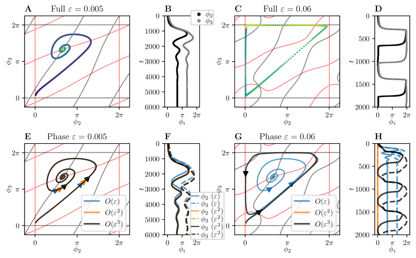
Figure 1: Comparison of the full (top row) and reduced (bottom row) CGL models. All panels show the corresponding nullclines of the $O(\varepsilon^{3})$ reduced model. A: Phase difference estimate of the full model dynamics at $\varepsilon=0.005$. Lighter shades indicate later times. E: The corresponding reduced models ($O(\varepsilon)$ blue, $O(\varepsilon^{2})$ orange, and $O(\varepsilon^{3})$ black). Arrows indicate movement in forward time. Note that all phase models coincide. B, F: Corresponding plots over time of the full model and reduced model, respectively. C, D, full and reduced model dynamics, respectively for $\varepsilon=0.06$. D, H: corresponding plots over time of the full and reduced models, respectively. Parameters: $d=0.9$, $\sigma=0.1$, $\rho=0.15$, and $\mu=1$.

We show comparisons between the full and reduced versions of the CGL model in Figure 1. The top row shows phase estimates of the full model for $\varepsilon=0.005$ (A) and $\varepsilon=0.06$ (C), where later shades correspond to later times. The bottom row shows the $O(\varepsilon)$ (blue), $O(\varepsilon^{2})$ (orange), and $O(\varepsilon^{3})$ (black) phase models exhibiting qualitatively similar dynamics at $\varepsilon=0.005$ (E) and $\varepsilon=0.06$ (G), respectively. Corresponding time traces are shown to the right of each portrait, e.g., panel B corresponds to A, and F corresponds to E.

At $\varepsilon=0.005$, the full model tends towards an asymptotically stable splay state when initialized near synchrony with phases $(\phi_{2},\phi_{3})=(0.05,0.25)$ (A,B, where $\phi_{i}\in[0,2\pi)$). With the same initial values, all $O(\varepsilon)$ (blue), $O(\varepsilon^{2})$ (orange), and $O(\varepsilon^{3})$ (black) phase models coincide with each other and with the full model as expected (E,F). For greater values of $\varepsilon$, the full model splay state loses stability and the phase differences converge towards a limit cycle attractor (C,D). Only the $O(\varepsilon^{3})$ (black) phase model exhibits a similar limit cycle oscillation, while the $O(\varepsilon)$ (blue) phase model dynamics does not change, and the $O(\varepsilon^{2})$ (orange) phase model simply converges to synchrony due to changes in the underlying basin of attraction (G,H).

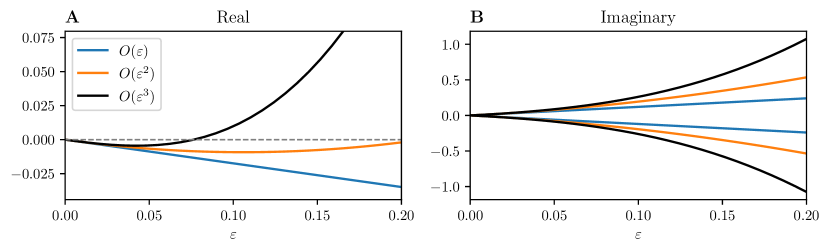
Figure 2: Real (A) and imaginary (B) parts of the eigenvalues of the Jacobian matrix evaluated at the splay state in the reduced CGL models. Blue: $O(\varepsilon)$, orange: $O(\varepsilon^{2})$, black: $O(\varepsilon^{3})$. Parameters are identical to those used in Figure 1.

Note that even though both $O(\varepsilon^{2})$ and $O(\varepsilon^{3})$ terms contain 3-body interactions, only the $O(\varepsilon^{3})$ phase model reproduces limit cycle behavior. Thus, this example demonstrates that $N$-body interactions per se are not always sufficient to capture the dynamics of the original model and that additional correction terms may be necessary.

The stability of the splay state is straightforward to calculate using the reduced model because we only the eigenvalues of the Jacobian matrix evaluated at the splay state $(\phi_{2},\phi_{3})=(2\pi/3,4\pi/3)$ need to be known. By using the Fourier expansion of the $\mathcal{H}$ functions, only derivatives of sinusoids are required to compute the Jacobian, and this derivative can be taken rapidly without the need for estimates such as finite differences. The result of this analysis is shown in 2. The left and right panels show the real and imaginary parts of the eigenvalues, respectively. While $O(\varepsilon^{2})$ (orange) does eventually lose stability, it occurs at a 4-fold greater coupling strength than the full or $O(\varepsilon^{3})$ models.

5 Thalamic Model

We now apply the method to a set of $N=3$ synaptically coupled conductance-based thalamic neuron models from [56]. These results extend our previous work where we applied a strongly coupled phase reduction method for $N=2$ thalamic models [50].

Table 1: Thalamic model parameter values.

Parameter	Value
$C$	$1\text{\,}\mathrm{\SIUnitSymbolMicro}\mathrm{F}\mathrm{/}\mathrm{c}\mathrm{m}^{2}$
$E_{k}$	$-90\text{\,}\mathrm{m}\mathrm{V}$
$E_{\text{Na}}$	$50\text{\,}\mathrm{m}\mathrm{V}$
$E_{\text{t}}$	$0\text{\,}\mathrm{m}\mathrm{V}$
$E_{\text{L}}$	$-70\text{\,}\mathrm{m}\mathrm{V}$
$E_{\text{syn}}$	$0\text{\,}\mathrm{m}\mathrm{V}$ (Figure 3) or $-100\text{\,}\mathrm{m}\mathrm{V}$ (Figure 5)
$g_{\text{L}}$	$0.05\text{\,}\mathrm{m}\mathrm{S}\mathrm{/}\mathrm{c}\mathrm{m}^{2}$
$g_{\text{K}}$	$5\text{\,}\mathrm{m}\mathrm{S}\mathrm{/}\mathrm{c}\mathrm{m}^{2}$
$g_{\text{Na}}$	$3\text{\,}\mathrm{m}\mathrm{S}\mathrm{/}\mathrm{c}\mathrm{m}^{2}$
$g_{\text{syn}}\equiv\varepsilon$	$0\text{\,}\mathrm{m}\mathrm{S}\mathrm{/}\mathrm{c}\mathrm{m}^{2}0.027\text{\,}\mathrm{m}\mathrm{S}\mathrm{/}\mathrm{c}\mathrm{m}^{2}$
$\alpha$	3
$\beta$	2
$\sigma_{T}$	0.8
$V_{\text{T}}$	$20\text{\,}\mathrm{m}\mathrm{V}$
$I_{\text{app}}$	$0.8\text{\,}\mathrm{\SIUnitSymbolMicro}\mathrm{A}\mathrm{/}\mathrm{c}\mathrm{m}^{2}$ (Figure 3) or $0.6\text{\,}\mathrm{\SIUnitSymbolMicro}\mathrm{A}\mathrm{/}\mathrm{c}\mathrm{m}^{2}$ (Figure 5)

The thalamic model is given by the equations,

$$\frac{dV_{i}}{dt} =-(I_{\text{L}}(V_{i})+I_{\text{Na}}(V_{i})+I_{\text{K}}(V_{i})+I_{\text{T}}(V_{i})+\frac{g_{\text{syn}}}{N}\sum_{j=1}^{N}a_{ij}w_{j}(V_{i}-E_{\text{syn}})-I_{\text{app}})/C,$$

$$\frac{dh_{i}}{dt} =(h_{\infty}(V_{i})-h_{i})/\tau_{h}(V_{i}),$$

$$\frac{dr_{i}}{dt} =(r_{\infty}(V_{i})-r_{i})/\tau_{r}(V_{i}),$$

$$\frac{dw_{i}}{dt} =\alpha(1-w_{i})/(1+\exp((V_{i}-V_{\text{T}})/\sigma_{T}))-\beta w_{i},$$

where $i=1,\ldots,3$, and $a_{ii}=0$ and $a_{ij}=1$ otherwise. Remaining equations are in Appendix B and all parameters are shown in Table 1. Given neuron $i$, the coupling term in the voltage variable $V_{i}$ is given by the average excitatory effect of the synaptic variables $w_{j}$ without self coupling. The synaptic conductance parameter $g_{\text{syn}}$ sets the overall coupling strength and is identical to the coupling strength parameter $\varepsilon$.

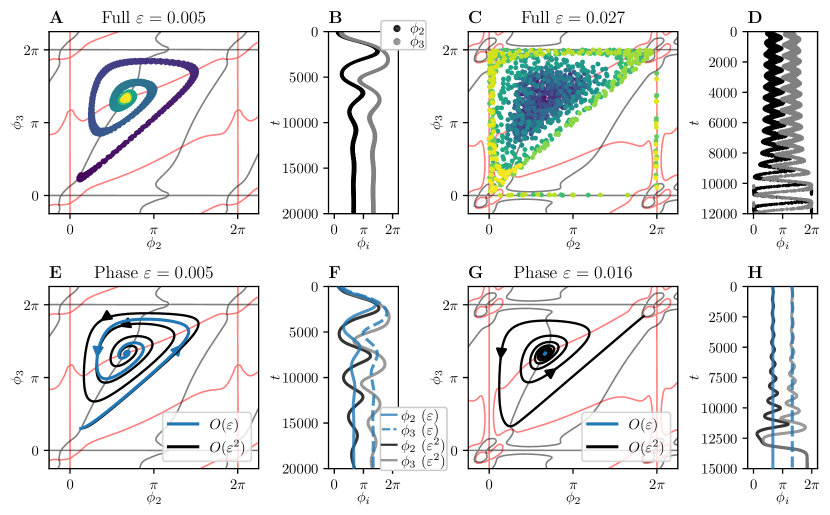
Figure 3: Comparison of the full (top row) and reduced (bottom row) thalamic models. All panels show the corresponding nullclines of the $O(\varepsilon^{2})$ reduced model. A: Phase difference estimate of the full model dynamics. Lighter shades indicate later times. E: The reduced models ($O(\varepsilon)$ blue and $O(\varepsilon^{2})$ black) at the approximate corresponding coupling strength. Note that the $O(\varepsilon)$ model remains at the splay state. Arrows indicate movement in forward time. B, F: Corresponding plots over time of the full model and reduced model, respectively. C, D, full and reduced model dynamics, respectively. D, H: corresponding plots over time of the full and reduced models, respectively. Parameters as in Table 1 with $E_{\text{syn}}=$0\text{\,}\mathrm{m}\mathrm{V}$$ and $I_{\text{app}}=$0.8\text{\,}\mu\mathrm{A}\mathrm{/}\mathrm{c}\mathrm{m}^{2}$$

We compare the reduced and full versions of the thalamic model in Figure 3, where the parameters are chosen as in Table 1 with with $E_{\text{syn}}=$0\text{\,}\mathrm{m}\mathrm{V}$$ and $I_{\text{app}}=$0.8\text{\,}\mu\mathrm{A}\mathrm{/}\mathrm{c}\mathrm{m}^{2}$$. for this figure are in table 1 The top row shows phase estimates of the full model for $\varepsilon=0.005$ (A) and $\varepsilon=0.027$ (C), where lighter shades correspond to later times. The bottom row shows the $O(\varepsilon)$ (blue) and $O(\varepsilon^{2})$ (black) phase models exhibiting qualitatively similar phase dynamics at $\varepsilon=0.005$ (E) and $\varepsilon=0.016$ (G), respectively. Corresponding time traces are shown to the right of each portrait, e.g., panel B corresponds to A, and F corresponds to E.

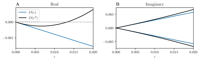
Figure 4: Real (A) and imaginary (B) parts of the eigenvalues of the Jacobian matrix evaluated at the splay state in the reduced thalamic models. Blue: $O(\varepsilon)$, orange: $O(\varepsilon^{2})$, black: $O(\varepsilon^{3})$. Parameters are identical to those used in Figure 3.

At $\varepsilon=0.005$, the full model phase differences tend towards an asymptotically stable splay state when initialized near synchrony with phases $(\phi_{2},\phi_{3})=(0.4,1)$ (A,B, where $\phi_{i}\in[0,2\pi)$). With the same initial values, all $O(\varepsilon)$ (blue), $O(\varepsilon^{2})$ (orange), and $O(\varepsilon^{3})$ (black) phase models coincide with the full model at as expected (E,F).

For greater values of $\varepsilon$, phase differences in the full model asymptotically tend towards a limit cycle oscillation (C,D) and the $O(\varepsilon^{2})$ reduced model tends towards synchrony. While the asymptotic dynamics differ, we nevertheless capture the loss of stability in the splay state. Real and imaginary parts of the Jacobian evaluated at the splay state is shown in Figure 3.

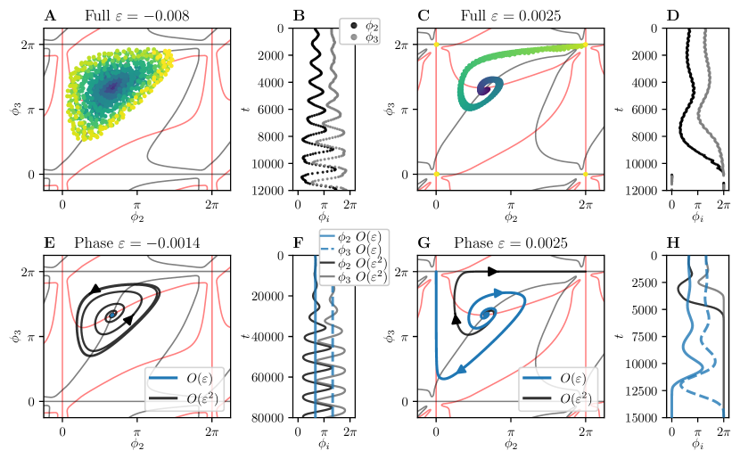
Figure 5: Comparison of the full (top row) and reduced (bottom row) thalamic models. All panels show the corresponding nullclines of the $O(\varepsilon^{2})$ reduced model. A: Phase difference estimate of the full model dynamics. Lighter shades indicate later times. E: The reduced models ($O(\varepsilon)$ blue and $O(\varepsilon^{2})$ black) at the approximate corresponding coupling strength. Note that the $O(\varepsilon)$ model remains at the splay state. Arrows indicate movement in forward time. B, F: Corresponding plots over time of the full model and reduced model, respectively. C, D, full and reduced model dynamics, respectively. D, H: corresponding plots over time of the full and reduced models, respectively. Parameters as in Table 1 with $E_{\text{syn}}=$-100\text{\,}\mathrm{m}\mathrm{V}$$ and $I_{\text{app}}=$0.6\text{\,}\mu\mathrm{A}\mathrm{/}\mathrm{c}\mathrm{m}^{2}$$

To further demonstrate the utility of our method, we show the phase reduction of the thalamic model for a different set of synaptic parameters: $E_{\text{syn}}=0$ and $\varepsilon<0$. This choice is less biologically relevant because it corresponds to an excitatory chemical synapse with a negative conductance, but the goal of this example is to show that the reduced model can capture additional nonlinear dynamics in a model more complex than the CGL model.

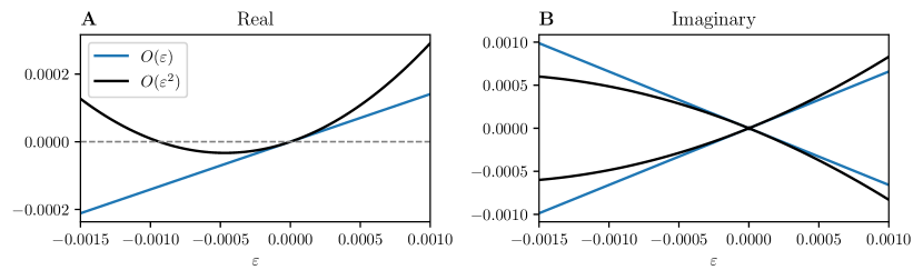
Figure 6: Real (A) and imaginary (B) parts of the eigenvalues of the Jacobian matrix evaluated at the splay state in the reduced thalamic models. Blue: $O(\varepsilon)$, orange: $O(\varepsilon^{2})$, black: $O(\varepsilon^{3})$. Parameters are identical to those used in Figure 5.

Comparisons between the full and reduced versions of the thalamic model for this new parameter set are shown in Figure 5. The top row shows phase estimates of the full model for $\varepsilon=-0.008$ (A) and $\varepsilon=0.0025$ (C), where lighter shades correspond to later times. The bottom row shows the $O(\varepsilon)$ (blue) and $O(\varepsilon^{2})$ (black) phase models exhibiting qualitatively similar phase dynamics at $\varepsilon=-0.0014$ (E) and $\varepsilon=0.0025$ (G), respectively. Corresponding time traces are shown to the right of each portrait, e.g., panel B corresponds to A, and F corresponds to E.

The right column of Figure 5 (panels C,D and G,H) serves as a sanity check, where $\varepsilon>0$ puts us back in a biologically realistic regime. The full and reduced models all tend towards synchrony, however, the $O(\varepsilon^{2})$ model (black) captures the transient dynamics more accurately than the $O(\varepsilon)$ model.

At $\varepsilon=-0.008$, the full model phase differences exhibit a loss of stability in the splay state and the asymptotic dynamics tend towards a limit cycle (A,B). The $O(\varepsilon^{2})$ reduced model captures this behavior (E,F, black), whereas the $O(\varepsilon)$ reduced model does not (E,F, blue). Note the considerable nonlinearity in the phase difference dynamics as a function of $\varepsilon$. Despite the small size of $\varepsilon$, the $O(\varepsilon)$ and $O(\varepsilon^{2})$ dynamics differ substantially.

This example is affected by a nearby saddle-node on an invariant cycle (SNIC) bifurcation, which occurs just below the applied current value of $I_{\text{app}}=$0.6\text{\,}\mu\mathrm{A}\mathrm{/}\mathrm{c}\mathrm{m}^{2}$$, and reminds us that “small” $\varepsilon$ is relative. The first example of the thalamic model (Figure 3) uses much greater values of $\varepsilon=0.005$ and $\varepsilon=0.027$, the latter being an order of magnitude greater than in the current example (Figure 5). The proximity to a SNIC also highlights the shortcomings with our second assumption, where we use first order averaging. The reciprocal of our period is $1/T=1/$44\text{\,}\mathrm{m}\mathrm{s}$\approx 0.023$, which places an approximate upper bound on the coupling strength $\varepsilon$, which must be much smaller than $1/T$ [35].

Nevertheless, we can compute changes in the stability of the splay state as in the previous examples. The real and imaginary parts of the eigenvalues of the Jacobian matrix evaluated at the splay state is shown in Figure 6. The $O(\varepsilon^{2})$ model captures the loss in stability while the $O(\varepsilon)$ model does not.

6 Discussion

In summary, we derived coupling functions that capture higher-order $N$-body interactions. We applied this method to two systems, the CGL model and a thalamic neuron model. While we did not consider heterogeneity, the formulation allows for the vector fields to be entirely different, so long as the oscillator periods are similar in the absence of coupling. Despite only considering pairwise interactions in the original systems, we found that higher-order terms were necessary to reproduce the dynamics of the original system. In the CGL model, even though the $O(\varepsilon^{2})$ reduced model contained 3-body interactions, it was the $O(\varepsilon^{3})$ reduced model (which also contains 3-body interactions) that could capture additional nonlinearities, suggesting that in general, $N$-body interactions per se are not always sufficient for accuracy. In the thalamic model, we considered two examples, the first at $I_{\text{app}}=$0.8\text{\,}\mu\mathrm{A}\mathrm{/}\mathrm{c}\mathrm{m}^{2}$$ $E_{\text{syn}}=-100$ and the second at $I_{\text{app}}=$0.6\text{\,}\mu\mathrm{A}\mathrm{/}\mathrm{c}\mathrm{m}^{2}$$ $E_{\text{syn}}=0$. In the first example, we captured the loss in stability of the splay state using the $O(\varepsilon^{2})$ model. In the second example, we observed limit cycle behavior in the phase difference of the full model by taking $g_{\text{syn}}\equiv\varepsilon<0$ and exploring beyond a biologically relevant parameter regime. The $O(\varepsilon^{2})$ reduced model captured this limit cycle behavior. The difference in $\varepsilon$ values between the full and reduced models to capture similar behaviors was notably different from the previous examples. This difference is likely due to the existence of a SNIC bifurcation just below the parameter value $I_{\text{app}}=$0.6\text{\,}\mu\mathrm{A}\mathrm{/}\mathrm{c}\mathrm{m}^{2}$$.

Our method is both a generalization of existing methods that consider higher-order phase interactions and a general framework from which to study higher-order effects. For example, a higher-order reduced model is derived using the Haken-Kelso-Bunz (HKB) equation in [38]. The higher-order terms are the lowest-order Fourier terms of our $\mathcal{H}$ functions, thus the same questions of existence can be answered with our method and further explored with additional Fourier terms and multi-body interactions. Larger networks of the HKB equation that consider interactions well beyond dyadic [74] fit comfortably within the limitations of our method (see Section 6.1 below for details). Similarly, there is no restriction to applying our method to questions of coordinated movement, e.g., [27], or studies of coupled population dynamics [41].

Our method may aid in addressing questions of synchrony and phase-locking in general finite populations of coupled oscillators with heterogeneity where order parameters are typically used. For example, the heterogeneous systems and coupling functions considered in [2] can not exhibit synchrony and a “bounded synchronization” measurement [23] is necessary. Our method could provide a far more detailed understanding of the bounded synchronization state alongside other possible phase-locked states. Moreover, similar questions could be asked in much more realistic and complex neurobiological models.

6.1 Limitations

We begin with limits related to our implementation. As mentioned in the text, if the $\mathcal{H}$ functions have a low Nyquist frequency, then a Fourier truncation can be used to greatly reduce the time complexity and memory requirements of our method (see Appendix A.1). In particular, knowledge of the exact types of functions that appear for each order is a significant part of this computational efficiency. However, the current implementation has only up to order $O(\varepsilon^{3})$ implemented for the Fourier method. While it is clear that there is a pattern in the types of separable and non-separable functions that appear in the Fourier terms as a function of higher orders, we have not precisely determined a formula for this pattern at the time of this writing. Once the pattern is fully understood, it will be possible to determine significantly higher-order interaction terms using the Fourier truncation.

Limitations related to the reduction method outside of our implementation center around the two key assumptions that make the derivation of this method possible. First, we assume that the timescale of phase $\theta_{i}-t$ (i.e., the phase equation after subtracting the moving frame) differs sufficiently from the timescale of the functions $p_{i}^{(k)}$ (the expansion terms of the isostable coordinate $\psi_{i}$), such that $\theta_{i}$ terms can be taken out of a time integral. This assumption is reasonable for at least moderate values of $\varepsilon$ up to $\varepsilon=0.06$ in our examples, where the phase difference variables $\phi_{i}$ tend to vary relatively slowly. However, additional work must be done to more carefully examine this assumption for use in greater $\varepsilon$.

Second, we use first order averaging, which is technically valid for small $\varepsilon$ comparable to those used in weak coupling theory. This limitation is especially apparent in the last example, where the thalamic model is near a SNIC bifurcation and the reciprocal of the period ($1/$44\text{\,}\mathrm{m}\mathrm{s}$\approx 0.023$) places an approximate upper bound on the coupling strength $\varepsilon$, as $\varepsilon$ must be much smaller than $1/T$ [35]. This is a good example of where higher-order averaging methods [34, 35] could be used. In addition, we have observed phase drift in the full model (data not shown) in a manner that may not be possible to capture in the current formulation. For example, with $N=3$ homogeneous oscillators and some values of $\varepsilon$, two oscillators synchronize and the third exhibits a phase drift, effectively resulting in a 2 oscillator system with a drift in the remaining phase difference. In our formulation, a single phase difference equation can not exhibit drift without heterogeneity. If this effect is due to resonance, it could be captured with higher-order averaging.

7 Acknowledgments

The authors acknowledge support under the National Science Foundation Grant No. NSF-2140527 (DW).

Appendix A Numerical Details for Computing Higher-Order Interaction Functions

Recall the non-autonomous version of the phase equation from the text:

$$\dot{\hat{\theta}}_{j}=\sum_{k=1}^{\infty}\sum_{j_{1},\ldots,j_{k}}\varepsilon^{k}\hat{h}_{j,j_{1},\ldots,j_{k}}^{(k)}(\hat{\theta}_{j}+t,\hat{\theta}_{j_{1}}+t\ldots,\hat{\theta}_{j_{k}}+t).$$

Note that we can abstract and rewrite the phase equation as

$$\dot{\hat{\theta}}_{j}=\sum_{k=1}^{\infty}\varepsilon^{k}\bar{h}_{j}^{(k)}(\hat{\theta}_{1}+t,\ldots,\hat{\theta}_{N}+t),$$

where $\bar{h}_{j}^{(k)}(\hat{\theta}_{1}+t,\ldots,\hat{\theta}_{N}+t)=\sum_{j_{1},\ldots,j_{k}}\varepsilon^{k}\hat{h}_{j,j_{1},\ldots,j_{k}}^{(k)}(\hat{\theta}_{j}+t,\hat{\theta}_{j_{1}}+t\ldots,\hat{\theta}_{j_{k}}+t)$ because the right-hand side will always depend on all oscillators. When we apply averaging, assuming we can interchange sums and integrals, we arrive at

$$\dot{\theta}_{j}=\frac{1}{T}\sum_{k=1}^{\infty}\int_{0}^{T}\bar{h}_{j}^{(k)}(\theta_{1}+t,\ldots,\theta_{N}+t)\,\mathrm{d}t.$$

Given a function of $N$ variables, the average integral is straightforward to calculate, but the integral requires knowledge of the function on a grid. For $N$ variables and $K$ points in the integration mesh for each axis, the grid is of size $(K,\ldots,K)\in\mathbb{Z}^{N}$ for some $K$ sufficiently large. This means evaluating the time-average integral on a grid of size $K^{N}$, which becomes rapidly intractable for even small $K$ and $N$. In the CGL model, $K=200$ and in the thalamic model, $K=1000$ or more. Even with small changes to these modest numbers, the number of calculations and memory requirements increase exponentially. Thus, one option is to exploit the periodicity of the underlying functions and express them in terms of their Fourier coefficients, which are significantly more memory-efficient and easier to calculate.

A.1 Option 1: Averaging in Terms of Fourier Coefficients

In cases where the response functions ($\mathcal{Z}$ and $\mathcal{I}$) and Floquet eigenfunctions have low Nyquist frequencies, only a small number of Fourier coefficients are needed to accurately reproduce the functions. While the following method does not apply to all cases, it is nevertheless an option that can dramatically improve computation times when it does apply, such as in the CGL model.

Given order $k$, define $\bm{\Theta}=(\theta_{1},\ldots,\theta_{N})$ and $\bm{1}=(1,\ldots,1)$. Consider the $N$-dimensional Fourier expansion of the integrand:

$$\int_{0}^{T}\bar{h}_{j}^{(k)}(\theta_{1}+t,\ldots,\theta_{N}+t)\,\mathrm{d}t=\int_{0}^{T}\sum_{\bm{m}\in\mathbb{Z}^{N}}c_{j,k,\bm{m}}e^{i\bm{m}\cdot(\bm{\Theta}+\bm{1}t)}\,\mathrm{d}t,$$

where $c_{j,k,\bm{m}}$ are the Fourier coefficients given oscillator $j$ and order $k$. Let the coordinates of $\bm{m}$ be given by $\bm{m}=(m_{1},m_{2},\ldots,m_{N})$. We simplify this integral using straightforward integral properties and orthogonality of the Fourier basis:

$$\begin{split}\int_{0}^{T}\sum_{\bm{m}\in\mathbb{Z}^{N}}c_{i,k,\bm{m}}e^{i\bm{m}\cdot(\bm{\Theta}+\bm{1}t)}\,\mathrm{d}t&=\sum_{\bm{m}\in\mathbb{Z}^{N}}\int_{0}^{T}c_{i,k,\bm{m}}e^{i\bm{m}\cdot(\bm{\Theta}+\bm{1}t)}\,\mathrm{d}t\\ &=\sum_{\bm{m}\in\mathbb{Z}^{N}}c_{i,k,\bm{m}}e^{i\bm{m}\cdot\bm{\Theta}}\int_{0}^{T}e^{i\bm{m}\cdot\bm{1}t}\,\mathrm{d}t\\ &=\sum_{\bm{m}\cdot\bm{1}=0}c_{i,k,\bm{m}}e^{i\bm{m}\cdot\bm{\Theta}}.\end{split}$$ (33)

That is, the only integral terms that remain are those such that the index vector $\bm{m}$ is orthogonal to the vector $\bm{1}$, and the integral of those surviving terms trivially evaluate to the scalar 1. Thus, the question of computing the average in time is simply a matter of computing the set of Fourier coefficients and extracting the relevant subset. If the number of oscillators $N$ and mesh size $K$ are large, then the desired averaged function in its final form can be taken as above, otherwise the desired functions can be found by the inverse Fourier transform.

Claim: The right-hand side of (33) depends on $N-1$ variables

Without loss of generality, suppose $j=1$. Now consider the change of variables $s=\theta_{1}+t$ and recall that $\phi_{i}=\theta_{i}-\theta_{1}$. Then rewriting (33) yields

$$\sum_{\bm{m}\in\mathbb{Z}^{N}}c_{1,k,\bm{m}}\int_{0}^{T}e^{i\bm{m}\cdot(s,\phi_{2}+s,\ldots,\phi_{N}+s)}\,\mathrm{d}s =\sum_{\bm{m}\in\mathbb{Z}^{N}}c_{1,k,\bm{m}}\int_{0}^{T}e^{i\left[m_{1}s+m_{2}(\phi_{2}+s)+\cdots+m_{N}(\phi_{N}+s)\right]}\,\mathrm{d}s$$

$$=\sum_{\bm{m}\in\mathbb{Z}^{N}}c_{1,k,\bm{m}}e^{i(m_{2}\phi_{2}+\cdots+m_{N}\phi_{N})}\int_{0}^{T}e^{is\bm{m}\cdot\bm{1}}\,\mathrm{d}s$$

$$=\sum_{\bm{m}\cdot\bm{1}=0}c_{1,k,\bm{m}}e^{i(m_{2}\phi_{2}+\cdots+m_{N}\phi_{N})},$$

where the last lines uses the orthogonality of the Fourier basis to evaluate the integral. Thus, we may easily evaluate (33) for $N-1$ phase differences by evaluating any one coordinate at zero.

While (33) is computationally efficient, we once again find that evaluating the underlying $N$-dimensional function to compute the Fourier coefficients of (33) requires significant amounts of memory. For example, evaluating an $N$ dimensional function on a mesh size of $K$ again requires $N^{K}$ points prior to taking the Fourier coefficient. So we seek an additional reduction in memory.

Using Separability to Reduce Memory Requirements

Fortunately, our interaction functions are mostly separable, colloquially speaking. That is, suppose we are given oscillator $i$, order $k$, and oscillators $(\theta_{j_{1}},\ldots,\theta_{j_{k}})$. Together, they give us the function in the summation of (26), which we recall to be $h^{(k)}_{i,j_{1},\ldots,j_{k}}(\theta_{i},\theta_{j_{1}},\ldots,\theta_{j_{k}})$. This function contains a sum of several functions that depend on the variables $(\theta_{i},\theta_{j_{1}},\ldots,\theta_{j_{k}})$. For each term inside $h^{(k)}_{i,j_{1},\ldots,j_{k}}(\theta_{i},\theta_{j_{1}},\ldots,\theta_{j_{k}})$, at best we can separate the term into $k$ functions of one variable. At worst, we can separate the term into $k-1$ functions of two variables. Note that we generally expect such inseparable functions to exist because $\hat{h}$ depends directly on $g_{i,j_{\ell},\alpha,\beta,\gamma,\delta}^{(k)}$, which is a function of two variables that can not be separated.

Suppose we pick a term $\zeta(\theta_{i},\theta_{j_{1}},\ldots,\theta_{j_{k}})$ which is only separable into functions of two variables:

$$\zeta(\theta_{i},\theta_{j_{1}},\ldots,\theta_{j_{k}})=\zeta_{0}(\theta_{i},\theta_{j_{1}})\zeta_{1}(\theta_{j_{1}},\theta_{j_{2}})\cdots\zeta_{k-1}(\theta_{j_{k-2}},\theta_{j_{k-1}})\zeta_{k}(\theta_{j_{k-1}},\theta_{j_{k}}).$$

Then (replacing $i$ with $\ell_{0}$ so that we can let $i$ stand for the imaginary number)

$$\zeta(\theta_{j_{0}},\theta_{j_{1}},\ldots,\theta_{j_{k}}) =\sum_{(x_{0},x_{1})\in\mathbb{Z}^{2}}c_{x_{0}x_{1}}^{(0,1)}e^{i[x_{0}\theta_{j_{0}}+x_{1}\theta_{j_{1}}]}\cdots\sum_{(x_{k-1},x_{k})\in\mathbb{Z}^{2}}c_{x_{k-1}x_{k}}^{(k-1,k)}e^{i[x_{k-1}\theta_{j_{k-1}}+x_{k}\theta_{j_{k}}]}$$

$$=\sum_{\bm{m}\in\mathbb{Z}^{k}}c_{x_{0}x_{1}}^{(0,1)}\cdots c_{x_{k-1}x_{k}}^{(k-1,k)}e^{i[x_{0}\theta_{j_{0}}+\cdots+x_{k}\theta_{j_{k}}]}$$

$$=\sum_{\bm{m}\in\mathbb{Z}^{k}}c_{\bm{m}}e^{i\bm{m}\cdot\bm{\Theta}},$$

where $c_{\bm{m}}=c_{x_{0}x_{1}}^{(0,1)}c_{x_{1}x_{2}}^{(1,2)}\cdots c_{x_{k-1}x_{k}}^{(k-1,k)}$, $\bm{m}=(x_{0},x_{1},\ldots,x_{k})\in\mathbb{Z}^{k}$ and $\bm{\Theta}=(\theta_{j_{0}},\theta_{j_{1}},\ldots,\theta_{j_{k}})$. Now $c_{\bm{m}}$ is significantly more memory efficient to compute because it is a product of coefficients that can be rapidly obtained using only a 2-dimensional fast Fourier transform. We also typically expect to truncate the Fourier coefficients to at most a few dozen terms, e.g., choose $\bm{m}$ such that $\|\bm{m}\|_{1}\leq z$ for $z$ not too large. The choice of $z$ depends on the model in question, but as a rule of thumb we start with $z\approx 5$. The CGL model requires $z=4$ up to order $k=3$ and the thalamic model requires $z=15$ up to order $k=3$.

According to (33) the time-average integral only requires coefficients such that $\bm{m}\cdot\bm{1}=0$. Thus, between truncating each Fourier series and selecting the subset of coefficients that survive the integral, the above sum simplifies to

$$\int_{0}^{T}\zeta(\theta_{\ell}+t,\theta_{j_{1}}+t,\ldots,\theta_{j_{k}}+t)\,\mathrm{d}t\approx\sum_{\begin{subarray}{c}\bm{m}\cdot\bm{1}=0\\ \|\bm{m}\|_{1}\leq 5\end{subarray}}c_{\bm{m}}e^{i\bm{m}\cdot\bm{\Theta}}.$$

A.2 Option 2: Using an ODE Solver as an Adaptive Mesh

In cases where the response functions ($\mathcal{Z}$ and $\mathcal{I}$) and Floquet eigenfunctions have derivatives that greatly exceed their magnitudes, it is not possible to use only a small number of Fourier coefficients. Indeed, the thalamic model has a relatively large Nyquist frequency at order $O(ve^{4})$. For a uniform mesh, the number of points in the time-average integral grid $K$ exceeds $1\text{\times}{10}^{7}$, which is difficult to compute efficiently. Parallelizing this problem is further hindered by memory constraints.

Because the sharp peaks in the response functions and eigenfunctions tend to be in small regions of phase space, an adaptive mesh greatly reduces the number of integration points $K$. The most straightforward method is to use an ODE solver by rephrasing the time-average integration as an initial value problem. Given $k$, and $\theta_{1},\ldots,\theta_{N}$, rewrite

$$\begin{split}\mathcal{H}&=\frac{1}{T}\int_{0}^{T}\bar{h}_{j}^{(k)}(\theta_{1}+t,\ldots,\theta_{N}+t)\,\mathrm{d}t\end{split}$$

as

$$\begin{split}T\frac{d}{dt}\mathcal{H}(t)&=\bar{h}_{j}^{(k)}(\theta_{1}+t,\ldots,\theta_{N}+t),\quad\mathcal{H}(0)=0.\end{split}$$

Then the desired time-average is given by $\mathcal{H}(T)$. If needed, the mesh is provided by the ODE solver. We use the Python [63] implementation of LSODA.

A.3 Option 3: Brute Force and Parallelization

If all else fails, it is possible to brute force calculations of the $\mathcal{H}$ functions, especially if the network has $N\leq 3$ oscillators with only a few lower-order terms and a coarse mesh. Our Python implementation will attempt to use CPU parallelization, and if available, CUDA parallelization. Because the memory requirements grow exponentially as a function of mesh size, mesh sizes are typically restricted to 500 points for roughly 16GB of RAM. Running the code on a cluster with more CPUs is recommended (instructions are included in the repository with sample scripts).

Appendix B Thalamic Model

The remaining equations for the Thalamic model are

$$I_{\text{L}}(V)=g_{\text{L}}(V-E_{L}), \quad I_{\text{Na}}=g_{\text{Na}}hm_{\infty}^{3}(V)(V-E_{\text{Na}}),$$

$$I_{\text{K}}=0.75g_{\text{K}}(1-h)^{4}(V-E_{\text{K}}), \quad I_{\text{T}}=g_{\text{T}}rp_{\infty}^{2}(V)(V-E_{\text{T}}),$$

and

$$a_{h}(V)=0.128\exp(-(V+46)/18), \quad b_{h}(V)=4/(1+\exp(-(V+23)/5)),$$

$$m_{\infty}(V)=1/(1+\exp(-(V+37)/7)), \quad h_{\infty}(V)=1/(1+\exp((V+41)/4)),$$

$$r_{\infty}(V)=1/(1+\exp((V+84)/4)), \quad p_{\infty}(V)=1/(1+\exp(-(V+60)/6.2)),$$

$$\tau_{h}(V)=1/(a_{h}(V)+b_{h}(V)), \quad\tau_{r}(V)=28+\exp(-(V+25)/10.5).$$

References

• [1] The infinitesimal phase response curves of oscillators in piecewise smooth dynamical systems. European Journal of Applied Mathematics, 29(5):905–940, 2018.
• [2] Francesco Alderisio, Benoît G Bardy, and Mario Di Bernardo. Entrainment and synchronization in networks of rayleigh–van der pol oscillators with diffusive and haken–kelso–bunz couplings. Biological cybernetics, 110:151–169, 2016.
• [3] Claude Berge. Principles of combinatorics. Academic Press, 1971.
• [4] Christian Bick, Tobias Böhle, and Christian Kuehn. Multi-population phase oscillator networks with higher-order interactions. Nonlinear Differential Equations and Applications NoDEA, 29(6):64, 2022.
• [5] Robert J Butera Jr, John Rinzel, and Jeffrey C Smith. Models of respiratory rhythm generation in the pre-Bötzinger complex. ii. populations of coupled pacemaker neurons. J. Neurophysiol., 82(1):398–415, 1999.
• [6] Carmen C. Canavier and Srisairam Achuthan. Pulse coupled oscillators and the phase resetting curve. Math. Biosci., 226(2):77–96, 2010.
• [7] Carmen C Canavier, Fatma Gurel Kazanci, and Astrid A Prinz. Phase resetting curves allow for simple and accurate prediction of robust N:1 phase locking for strongly coupled neural oscillators. Biophys. J., 97(1):59–73, 2009.
• [8] Rishidev Chaudhuri, Kenneth Knoblauch, Marie-Alice Gariel, Henry Kennedy, and Xiao-Jing Wang. A large-scale circuit mechanism for hierarchical dynamical processing in the primate cortex. Neuron, 88(2):419–431, 2015.
• [9] Stephen Coombes. Neuronal networks with gap junctions: A study of piecewise linear planar neuron models. SIAM Journal on Applied Dynamical Systems, 7(3):1101–1129, 2008.
• [10] Stephen Coombes, Yi Ming Lai, Mustafa Şayli, and Ruediger Thul. Networks of piecewise linear neural mass models. European Journal of Applied Mathematics, 29(5):869–890, 2018.
• [11] Stephen Coombes, Ruediger Thul, and Kyle CA Wedgwood. Nonsmooth dynamics in spiking neuron models. Physica D: Nonlinear Phenomena, 241(22):2042–2057, 2012.
• [12] Marco Coraggio, Pietro De Lellis, and Mario di Bernardo. Convergence and synchronization in networks of piecewise-smooth systems via distributed discontinuous coupling. Automatica, 129:109596, 2021.
• [13] Jianxia Cui, Carmen C Canavier, and Robert J Butera. Functional phase response curves: a method for understanding synchronization of adapting neurons. J. Neurophysiol., 102(1):387–398, 2009.
• [14] JD Da Fonseca and Celso Vieira Abud. The kuramoto model revisited. Journal of Statistical Mechanics: Theory and Experiment, 2018(10):103204, 2018.
• [15] Irving R Epstein and John A Pojman. An introduction to nonlinear chemical dynamics: oscillations, waves, patterns, and chaos. Oxford University Press, 1998.
• [16] G. B. Ermentrout and D. H. Terman. Mathematical Foundations of Neuroscience, volume 35. Springer, New York, 2010.
• [17] G. Bard Ermentrout and David H. Terman. Mathematical foundations of neuroscience, volume 35 of Interdisciplinary Applied Mathematics. Springer, New York, 2010.
• [18] George Bard Ermentrout and Nancy Kopell. Frequency plateaus in a chain of weakly coupled oscillators, i. SIAM journal on Mathematical Analysis, 15(2):215–237, 1984.
• [19] Erik Genge, Erik Teichmann, Michael Rosenblum, and Arkady Pikovsky. High-order phase reduction for coupled oscillators. arXiv preprint arXiv:2007.14077, 2020.
• [20] Jorge Golowasch, Frank Buchholtz, Irving R Epstein, and E Marder. Contribution of individual ionic currents to activity of a model stomatogastric ganglion neuron. J. Neurophysiol., 67(2):341–349, 1992.
• [21] Martin Golubitsky, Leopold Matamba Messi, and Lucy E Spardy. Symmetry types and phase-shift synchrony in networks. Physica D: Nonlinear Phenomena, 320:9–18, 2016.
• [22] J. Guckenheimer. Isochrons and phaseless sets. Journal of Mathematical Biology, 1(3):259–273, 1975.
• [23] David J Hill and Jun Zhao. Global synchronization of complex dynamical networks with non-identical nodes. In 2008 47th IEEE Conference on Decision and Control, pages 817–822. IEEE, 2008.
• [24] Ian Hunter, Michael M Norton, Bolun Chen, Chris Simonetti, Maria Eleni Moustaka, Jonathan Touboul, and Seth Fraden. Pattern formation in a four-ring reaction-diffusion network with heterogeneity. Physical Review E, 105(2):024310, 2022.
• [25] E. M. Izhikevich. Dynamical Systems in Neuroscience: The Geometry of Excitability and Bursting. MIT Press, London, 2007.
• [26] Eugene M. Izhikevich. Dynamical systems in neuroscience: the geometry of excitability and bursting. Computational Neuroscience. MIT Press, Cambridge, MA, 2007.
• [27] JA Scott Kelso. Unifying large-and small-scale theories of coordination. Entropy, 23(5):537, 2021.
• [28] Nancy Kopell and G Bard Ermentrout. Symmetry and phaselocking in chains of weakly coupled oscillators. Communications on Pure and Applied Mathematics, 39(5):623–660, 1986.
• [29] Y. Kuramoto. Chemical oscillations, waves, and turbulence, volume 19 of Springer Series in Synergetics. Springer-Verlag, Berlin, 1984.
• [30] Y. Kuramoto. Chemical Oscillations, Waves, and Turbulence. Springer-Verlag, Berlin, 1984.
• [31] M. D. Kvalheim and S. Revzen. Existence and uniqueness of global koopman eigenfunctions for stable fixed points and periodic orbits. Physica D: Nonlinear Phenomena, 425:132959, 2021.
• [32] Iván León and Diego Pazó. Phase reduction beyond the first order: The case of the mean-field complex ginzburg-landau equation. Physical Review E, 100(1):012211, 2019.
• [33] Iván León and Diego Pazó. Enlarged kuramoto model: Secondary instability and transition to collective chaos. Physical Review E, 105(4):L042201, 2022.
• [34] Jaume Llibre, Douglas D. Novaes, and Marco A. Teixeira. Higher order averaging theory for finding periodic solutions via Brouwer degree. Nonlinearity, 27(3):563–583, 2014.
• [35] Marco Maggia, Sameh A Eisa, and Haithem E Taha. On higher-order averaging of time-periodic systems: reconciliation of two averaging techniques. Nonlinear Dynamics, 99(1):813–836, 2020.
• [36] Jan R Magnus and Heinz Neudecker. Matrix differential calculus with applications in statistics and econometrics. John Wiley & Sons, 2019.
• [37] Alexandre Mauroy, Igor Mezić, and Jeff Moehlis. Isostables, isochrons, and Koopman spectrum for the action–angle representation of stable fixed point dynamics. Physica D: Nonlinear Phenomena, 261:19–30, 2013.
• [38] Joseph McKinley, Mengsen Zhang, Alice Wead, Christine Williams, Emmanuelle Tognoli, and Christopher Beetle. Third party stabilization of unstable coordination in systems of coupled oscillators. In Journal of Physics: Conference Series, volume 2090, page 012167. IOP Publishing, 2021.
• [39] Aaron Meurer, Christopher P. Smith, Mateusz Paprocki, Ondřej Čertík, Sergey B. Kirpichev, Matthew Rocklin, AMiT Kumar, Sergiu Ivanov, Jason K. Moore, Sartaj Singh, Thilina Rathnayake, Sean Vig, Brian E. Granger, Richard P. Muller, Francesco Bonazzi, Harsh Gupta, Shivam Vats, Fredrik Johansson, Fabian Pedregosa, Matthew J. Curry, Andy R. Terrel, Štěpán Roučka, Ashutosh Saboo, Isuru Fernando, Sumith Kulal, Robert Cimrman, and Anthony Scopatz. Sympy: symbolic computing in python. PeerJ Computer Science, 3:e103, January 2017.
• [40] Igor Mezić. Spectrum of the koopman operator, spectral expansions in functional spaces, and state-space geometry. Journal of Nonlinear Science, 30(5):2091–2145, 2020.
• [41] Russell Milne and Frederic Guichard. Coupled phase-amplitude dynamics in heterogeneous metacommunities. Journal of Theoretical Biology, 523:110676, 2021.
• [42] Renato E. Mirollo and Steven H. Strogatz. Synchronization of pulse-coupled biological oscillators. SIAM J. Appl. Math., 50(6):1645–1662, 1990.
• [43] B. Monga, D. Wilson, T. Matchen, and J. Moehlis. Phase reduction and phase-based optimal control for biological systems: a tutorial. Biological Cybernetics, 113(1-2):11–46, 2019.
• [44] Rachel Nicks, Lucie Chambon, and Stephen Coombes. Clusters in nonsmooth oscillator networks. Physical Review E., 97(3):032213, 2018.
• [45] Edward Ott and Thomas M Antonsen. Low dimensional behavior of large systems of globally coupled oscillators. Chaos, 18(3):037113, 2008.
• [46] Youngmin Park. youngmp/nbody: v0.2.0-alpha, August 2023.
• [47] Youngmin Park and Bard Ermentrout. Weakly coupled oscillators in a slowly varying world. J. Comput. Neurosci., 40(3):269–281, 2016.
• [48] Youngmin Park and G Bard Ermentrout. A multiple timescales approach to bridging spiking-and population-level dynamics. Chaos: An Interdisciplinary Journal of Nonlinear Science, 28(8), 2018.
• [49] Youngmin Park, Stewart Heitmann, and G. Bard Ermentrout. The utility of phase models in studying neural synchronization. Computational Models of Brain and Behavior, pages 493–504, 2017.
• [50] Youngmin Park and Dan D Wilson. High-order accuracy computation of coupling functions for strongly coupled oscillators. SIAM Journal on Applied Dynamical Systems, 20(3):1464–1484, 2021.
• [51] Alberto Pérez-Cervera, Tere M Seara, and Gemma Huguet. Global phase-amplitude description of oscillatory dynamics via the parameterization method. arXiv preprint arXiv:2004.03647, 2020.
• [52] Charles S. Peskin. Mathematical aspects of heart physiology. Courant Institute of Mathematical Sciences, New York University, New York, 1975. Notes based on a course given at New York University during the year 1973/74.
• [53] Carsten K Pfeffer, Mingshan Xue, Miao He, Z Josh Huang, and Massimo Scanziani. Inhibition of inhibition in visual cortex: the logic of connections between molecularly distinct interneurons. Nature Neuroscience, 16(8):1068–1076, 2013.
• [54] B. Pietras and A. Daffertshofer. Network dynamics of coupled oscillators and phase reduction techniques. Physics Reports, 2019.
• [55] Michael Rosenblum and Arkady Pikovsky. Numerical phase reduction beyond the first order approximation. Chaos, 29(1):011105, 2019.
• [56] Jonathan E Rubin and David Terman. High frequency stimulation of the subthalamic nucleus eliminates pathological thalamic rhythmicity in a computational model. Journal of Computational Neuroscience, 16(3):211–235, 2004.
• [57] S. Shirasaka, W. Kurebayashi, and H. Nakao. Phase-amplitude reduction of transient dynamics far from attractors for limit-cycling systems. Chaos: An Interdisciplinary Journal of Nonlinear Science, 27(2):023119, 2017.
• [58] Per Sebastian Skardal and Alex Arenas. Higher order interactions in complex networks of phase oscillators promote abrupt synchronization switching. Communications Physics, 3(1):218, 2020.
• [59] Per Sebastian Skardal, Edward Ott, and Juan G Restrepo. Cluster synchrony in systems of coupled phase oscillators with higher-order coupling. Physical Review E, 84(3):036208, 2011.
• [60] Steven H Strogatz, Daniel M Abrams, Allan McRobie, Bruno Eckhardt, and Edward Ott. Crowd synchrony on the millennium bridge. Nature, 438(7064):43–44, 2005.
• [61] Takuma Tanaka and Toshio Aoyagi. Multistable attractors in a network of phase oscillators with three-body interactions. Physical Review Letters, 106(22):224101, 2011.
• [62] Corey Michael Thibeault and Narayan Srinivasa. Using a hybrid neuron in physiologically inspired models of the basal ganglia. Frontiers in Computational Neuroscience, 7:88, 2013.
• [63] Guido Van Rossum and Fred L. Drake. Python 3 Reference Manual. CreateSpace, Scotts Valley, CA, 2009.
• [64] K. C. A. Wedgwood, K. K. Lin, R. Thul, and S. Coombes. Phase-amplitude descriptions of neural oscillator models. The Journal of Mathematical Neuroscience, 3(1):2, 2013.
• [65] D. Wilson and B. Ermentrout. Greater accuracy and broadened applicability of phase reduction using isostable coordinates. Journal of Mathematical Biology, 76(1-2):37–66, 2018.
• [66] D. Wilson and B. Ermentrout. An operational definition of phase characterizes the transient response of perturbed limit cycle oscillators. SIAM Journal on Applied Dynamical Systems, 17(4):2516–2543, 2018.
• [67] D. Wilson and J. Moehlis. Isostable reduction of periodic orbits. Physical Review E, 94(5):052213, 2016.
• [68] D. Wilson and J. Moehlis. Recent advances in the analysis and control of large populations of neural oscillators. Annual Reviews in Control, 54:327–351, 2022.
• [69] Dan Wilson. Phase-amplitude reduction far beyond the weakly perturbed paradigm. Physical Review E., 101(2):022220, 2020.
• [70] Dan Wilson and Bard Ermentrout. Greater accuracy and broadened applicability of phase reduction using isostable coordinates. J. Math. Biol., 76(1-2):37–66, 2018.
• [71] Dan Wilson and Bard Ermentrout. Phase models beyond weak coupling. Physical Review Letters, 123(16):164101, 2019.
• [72] Arthur T Winfree. The geometry of biological time, volume 12. Springer Science & Business Media, 2001.
• [73] Yunliang Zang and Eve Marder. Neuronal morphology enhances robustness to perturbations of channel densities. Proceedings of the National Academy of Sciences, 120(8):e2219049120, Feb 2023.
• [74] Mengsen Zhang, Christopher Beetle, JA Scott Kelso, and Emmanuelle Tognoli. Connecting empirical phenomena and theoretical models of biological coordination across scales. Journal of the Royal Society Interface, 16(157):20190360, 2019.