Addressing Distribution Shift in RTB Markets
via Exponential Tilting

Abstract

Distribution shift in machine learning models can be a primary cause of performance degradation. This paper delves into the characteristics of these shifts, primarily motivated by Real-Time Bidding (RTB) market models. We emphasize the challenges posed by class imbalance and sample selection bias, both potent instigators of distribution shifts. This paper introduces the Exponential Tilt Reweighting Alignment (ExTRA) algorithm, as proposed by Maity et al. (2023), to address distribution shifts in data. The ExTRA method is designed to determine the importance weights on the source data, aiming to minimize the KL divergence between the weighted source and target datasets. A notable advantage of this method is its ability to operate using labeled source data and unlabeled target data. Through simulated real-world data, we investigate the nature of distribution shift and evaluate the applicacy of the proposed model.

1 Introduction

The dynamic nature of machine learning often presents a problem concerning distribution shifts, whereby the distributions of the source and target observations differ significantly (Quionero-Candela et al. (2009)). Such shifts can take various forms, from covariate shifts, where only the marginal distribution of the covariate $X$ alters, to label shifts, where only the marginal distribution of the label $Y$ changes, and even to more intricate variations like concept shifts, where both covariates and labels can deviate (Zhang et al. (2021)).

This phenomenon of distribution shift can lead to a significant drop in performance when a model trained solely on source data is subsequently applied to target data. Weighting methods are often considered to deal with distribution shifts (Shimodaira (2000), Maity et al. (2020)). To elaborate, let us consider that we have labeled data $(X,Y)$ with covariate $X$ and target $Y$ pairs. Assume that the joint data come from the distribution $P$. Machine learning models are designed to minimize the empirical risk, represented as

$${R}_{P}(f)={\operatorname*{\mathbb{E}}}_{P}l(f(X),Y)\approx\frac{1}{N}\sum_{i=1}^{N}l(f(X_{i}),Y_{i}),$$ (1)

where $f(\cdot)$ is the model and $l$ denotes the loss function. When dealing with distribution shifts, it is assumed that the target data originates from a different distribution, say $Q$. We further assume in the following that there exists density functions, $p$ and $q$, respectively for the measure $P$ and $Q$. Note that the expected risk in the target domain can be written as follows:

$${R}_{Q}(f) ={\operatorname*{\mathbb{E}}}_{Q}l(f(X),Y)=\int l(f(X),Y)dQ$$ (2)

$$=\int l(f(X),Y)\frac{q(X,Y)}{p(X,Y)}dP={\operatorname*{\mathbb{E}}}_{P}\Big{[}l(f(X),Y)\frac{q(X,Y)}{p(X,Y)}\Big{]}.$$

Since the ultimate goal of the model is to perform effectively on data drawn from the target distribution, we can improve the performance by minimizing the weighted empirical risk

$$\frac{1}{N}\sum_{(X_{i},Y_{i})\sim P}l(f(X_{i}),Y_{i})\frac{q(X_{i},Y_{i})}{p(X_{i},Y_{i})}.$$

In essence, weighting models aim to learn the importance weight, $\frac{q(X,Y)}{p(X,Y)}$ to adjust for the shift between the source and target distributions.

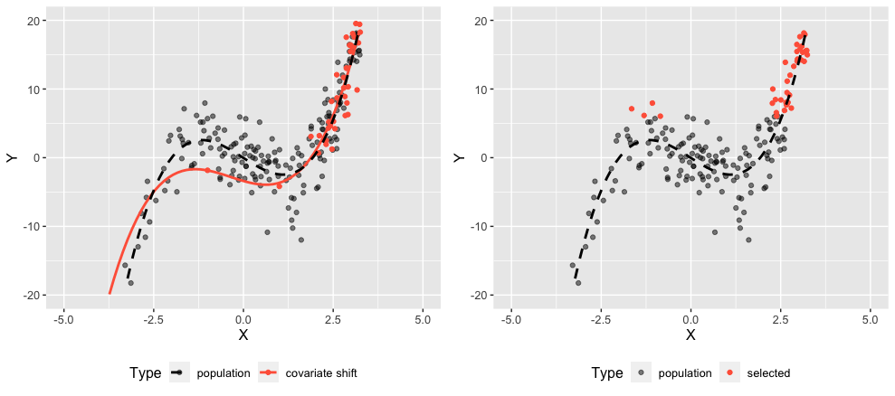
Figure 1: Illustration of distribution shift. (Left) Covariate Shift (Right) Sample selection bias

The left panel of Figure 1 illustrates an example of covariate shift. In such scenario, weights can be given as $q(X)/p(X)$ by marginal distribution of $X$ without observing $Y$. On the other hand, selection bias refers to a situation where sample selection is expected and correlated with $Y$. As can be seen in the right panel of Figure 1, it distorts the conditional distribution of $Y|X$, thereby significantly affecting the model. In the next section, we present class imbalance and sample selection bias as potential causes of distribution shifts. The rationale for considering these aspects stems from our motivating example where we treat the RTB market model as a binary classification problem. A detail of this perspective will be provided in Section 2. Weighting techniques may fall short when predicting in regions with scant information from the source domain. Phenomena such as adversarial examples proposed by Goodfellow et al. (2015) are well-documented. To address challenges in out-of-distribution scenarios, strategies like exploration (Osband et al. (2016)) and the adoption of robust models (Hendrycks & Dietterich (2019)) are often considered.

In a recent paper by Maity et al. (2023), the Exponential Tilt Reweighting Alignment (ExTRA) algorithm (Algorithm 1) is introduced as an approach to estimate the weight between the source and target domain. To this end, it solves a distribution matching technique, aiming to minimize the KL divergence between weighted source and target datasets. The goal of our study is to investigate the possibility of dealing distribution shift in RTB market model using the algorithm.

The rest of the paper is organized as follows: Section 2 introduces the distribution shift in RTB market model. Section 3 introduce the exponential tilt model and the main algorithm. Section 3 evaluates the outcomes of weighting under settings mirroring real market data. Section 5 concludes and suggests future directions.

2 Motivating Dataset: Real-Time Bidding (RTB)

RTB is a digital advertising method where ad impressions are auctioned in real-time, often in milliseconds, as a user loads an ad slot. What makes this mechanism intriguing from a machine learning standpoint lies in predicting, in split seconds, which advertisement will resonate most with the profile of the user based on various features. As the RTB market dynamics fluctuate and user behaviors shift over time, the underlying data distributions can change, introducing challenges for predictive models that were trained on historical data. The RTB market, therefore, provides a tangible and rich context to delve into the intricacies of managing distribution shifts in machine learning. In this section, we introduce two prominent characteristics of the market model: class imbalance and selection bias. To proceed with, we formulate the market model as prediction of the binary random variable indicating the utility of a bid opportunity given its features as covariate $X$.

Class imbalance is characterized by a significant rarity of one class compared to the other. In the realm of advertising, the probability of an impression leading to utility, such as app installations or in-app purchases, is remarkably low. For instance, expected app install probabilities often fall in the range of $10^{-3}$ to $10^{-5}$ or could be even lower. In the empirical risk minimization as expressed in eq (1), mis-classification errors of data instances from both classes are treated with equal importance. Consequently, it leads the classifier to be biased towards the majority class. As Wallace & Dahabreh (2013) points out, skewed class distribution in source data tends to produce unreliable class probability estimates, especially for minority class instances. To address class imbalance, various approaches can be considered. A straightforward sampling approach emphasizes the minority class by using a subset of the data. However, it might lead to selection bias and can adversely affect probability calibration for minority classes as indicated by Pozzolo et al. (2015). More general approach considers adjusting the loss function, which can systematically reshape the optimization objective. For instance, Fernando & Tsokos (2022) suggests dynamic weighting for minor classes, while Li et al. (2021) emphasizes misclassifications with the tilted loss. Careful evaluation of these approaches is crucial to assess their impact on model performance and generalization.

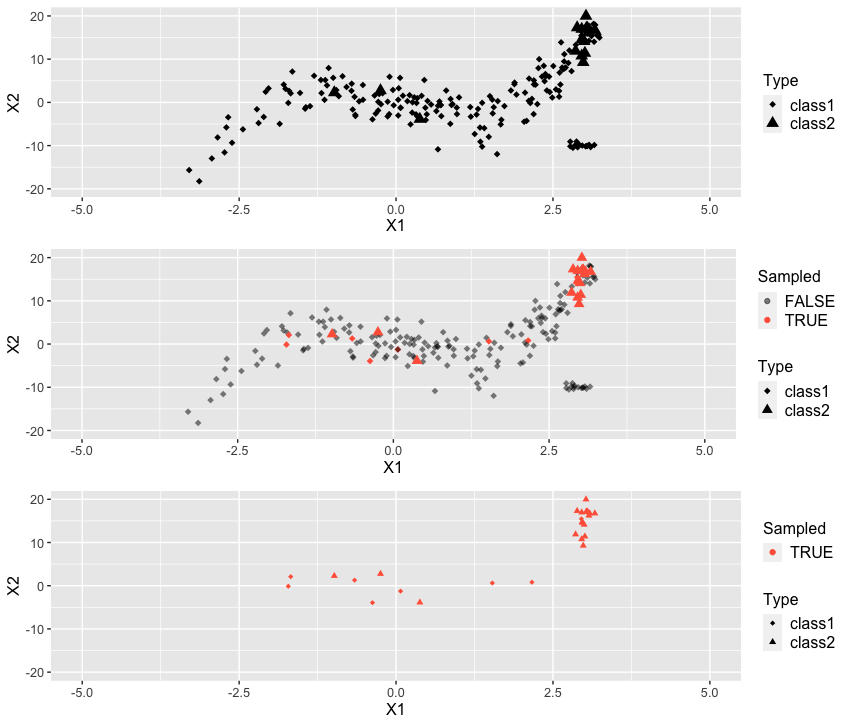
Figure 2: Selection bias in binary classification

A more straightforward cause of the distribution shift is the sample selection bias, where the sample selection process is dependent on the target variable $U$. To exemplify, consider a training model $p$ and data $(X,U)$, accompanied by a binary sample selection variable $V$; with $V=1$ indicating a selected sample, and $V=0$ otherwise. If the true joint distribution of $X$ and $U$ follows $p_{o}$,

$$p(X,U)=p_{o}(X,U|V=1)=p_{o}(U|X,V=1)p_{o}(X|V=1)$$

while for the test model $q$,

$$q(X,U)=p_{o}(X,U)=p_{o}(U|X)p_{o}(X).$$

The selection bias is incited by the dependence of $V$ on $U$. In the absence of this dependence, the scenario would simply be classified as a covariate shift. As illustrated in Figure 2, the selection bias can impact the model’s prediction $P(U|X,V=1)$, leading it to significantly differ from the true conditional distribution $P(U|X)$.

To describe the presence of selection bias in RTB market model, we define $U_{i}\in\{0,1\}$ the utility of request $i$ and $M_{i}\in\mathbb{M}$ the market condition of request $i$ as the random variables with proper distribution function and some measurable space $(\mathbb{M},\mathcal{M})$. The estimated utility $\operatorname*{\mathbb{E}}\operatorname*{\textit{U}}$ can be subsequently utilized to determine the optimal bid price in an optimization process. Given a specific user context, let $M$ represent the winning auction price. $\operatorname*{\textit{U}}$ is observable only when our bidding price $b$ exceeds $M$, meaning we win the auction. Thus, a sample is chosen when $M<b$. An estimator derived from the source set is given by $p:=\operatorname*{\mathbb{E}}_{\text{win}}(\operatorname*{\textit{U}})=P(\operatorname*{\textit{U}}=1|M<b)$. If we denote $\pi:=\operatorname*{\mathbb{E}}_{\text{total}}\operatorname*{\textit{U}}$ to be the true probability in the target domain, the following relationships hold:

$$p ={\operatorname*{\mathbb{P}}}_{\text{win}}(U=1)=\frac{\pi\cdot F_{1}(b)}{F(b)}$$ (3)

Here, $F_{1},F_{0}$ are conditional cdf of $M$ when $U=1$ and $U=0$, respectively. $F(b)=(1-\pi)F_{0}(b)+\pi F_{1}(b)$ signifies the marginal cdf of $M$. As (3) indicates, $p$ converges to $\pi$ as $b\to\infty$. This means that there will be no bias if we win all bids. For any bid price $b$, the $p$ equals $\pi$ when $F_{1}(b)=F_{0}(b)$. This suggests that if the market condition is independent of the utility, the selection bias disappears. In conclusion, distribution shifts, including covariate shifts, are intrinsically present in the process of model training. Yet, the existence of a dependency between market price and utility could exacerbate these shifts, adding a layer of selection bias that further distorts the distribution. In sum, when observing performance variations due to changes in budget levels, it’s crucial to consider and address these distribution shifts.

3 The Exponential Tilt Model

In this section, we explore the importance weighting approach, designed to classify the utility in target domains that differ from the original source datasets. The model aims to improve the prediction performance in these new domains by giving more weight to relevant samples, instead of just utilizing uniform source weights. While our approach aligns closely with the methods detailed in Maity et al. (2023), we provide a comprehensive overview for our discussion to be self-contained.

Problem setup We consider a binary classification problem where $U$ can take values of $0$ or $1$. One can easily extend it to $K$-class classification problem. Let $\mathcal{X}$ and $\mathcal{U}$ be the space of features and set of possible utility. We assume in the following that there exists a probability measures and associated densities for the source and target dataset. Let $P$ and $Q$ be probability distributions on $\operatorname*{\mathcal{X}}\times\operatorname*{\mathcal{U}}$ and $p$ and $q$ be the associated densities for the source and target domains.

The data we train on are exclusively ‘winning’ bids. Consequently, we have a ‘source domain’ with a labeled dataset $\{X_{\{W,i\}},U_{\{W,i\}}\}_{i=1}^{n_{W}}$ corresponding to winning bids. Here, the subscript ‘W’ represents the winning bids. In contrast, the ‘target domain’ encompasses all bid opportunities - both winning and losing. In this domain, only unlabeled samples $\{X_{\{T,i\}}\}_{i=1}^{n_{T}}$ are available. The subscript ‘T’ stands for the total bids. The goal of the ExTRA algorithm (Maity et al. (2023)) is to learn importance weights on samples from a source domain so that the weighted source samples mimic the target distribution. To make the learning of the weight function feasible, we introduce the following additional constraints on the domains.

The exponential tilt model We assume that there is a vector of sufficient statistics $T:\operatorname*{\mathcal{X}}\rightarrow\operatorname*{\mathbb{R}}^{p}$ and the parameters $\{\theta_{i}\in\operatorname*{\mathbb{R}},\alpha_{i}\in\operatorname*{\mathbb{R}}\}_{i\in\{0,1\}}$ such that

$$\log\frac{q(x,U=i)}{p(x,U=i)}=\theta_{i}^{\top}T(x)+\alpha_{i},\ i\in\{0,1\}.$$ (4)

This will assume $q(x,U=i)$ to be a member of the exponential family with base measure $p(x,U=i)$ and sufficient statistic $T$ nwhen normalized. We call (4) the exponential tilt model. It implies the importance weights between the source and target samples are

$$w(x,i)=\exp(\theta_{i}^{\top}T(x)+\alpha_{i}),\ i\in\{0,1\}.$$

Suppose the model is drawn from the selection bias assumption as discussed in Section 2 and let $p_{o}$ be the true joint distribution of $X$ and $U$. Under this setting, we can further expand the tilt model.

$$\frac{q(X,U)}{p(X,U)}=\frac{p_{o}(X,U)}{p_{o}(X,U|V=1)}=\frac{p_{o}(V=1)}{p_{o}(V=1|X,U)}.$$

To employ the weighting idea in eq (2), (4) can be written as

$$\frac{q(X,U)}{p(X,U)}=\begin{cases}\displaystyle\frac{p_{o}(V=1)}{p_{o}(V=1|X,U=0)}=e^{\theta_{0}^{\top}T(X)+\alpha_{0}}&\text{ if }U=0\\ \\ \displaystyle\frac{p_{o}(V=1)}{p_{o}(V=1|X,U=1)}=e^{\theta_{1}^{\top}T(X)+\alpha_{1}}&\text{ if }U=1\end{cases}.$$ (5)

Fitting the exponential tilt model Given the exponential tilt model in (4), the marginal density of the features in the target domain $q_{X}$ is represented as:

$$q_{X}\{x\}=\sum_{i=0,1}p(x,U=i)\exp{(\theta_{i}^{\top}T(x)+\alpha_{i})}.$$ (6)

From this formulation, the optimization problem for distribution matching, constrained to the integration of the marginal density equating to one, is described by:

$$\{{\operatorname*{\hat{\theta}}}_{i},{\operatorname*{\hat{\alpha}}}_{i}\}_{i\in\{0,1\}}\in \operatorname*{arg\,min}_{(\theta_{i},\alpha_{i})}\sum_{i=0,1}D\big{(}{\operatorname*{\hat{\textit{q}}}}_{X}\{x\}\|\operatorname*{\hat{\textit{p}}}\{x,U=i\}\exp{(\theta_{i}^{\top}T(x)+\alpha_{i})}\big{)}$$ (7)

$$\text{subject to }\int_{\mathcal{X}}{\sum_{i=0,1}\operatorname*{\hat{\textit{p}}}\{x,U=i\}\exp(\theta_{i}^{\top}T(x)+\alpha_{i})dx}=1$$

The choice of $D$ as a metric to measure the distance between distributions is flexible. Maity et al. (2023) demonstrated that using the Kullback-Leibler (KL) divergence allows the optimization to proceed without needing to estimate $p(x,U=i)$ or $q(x)$. Rather, it necessitates a probabilistic classifier, $\operatorname*{\hat{\eta}}_{W}=\{\operatorname*{\hat{\eta}}_{W,i}\}_{i\in\{0,1\}}$ trained from the source domain, which can be written as

$${\operatorname*{\hat{\eta}}}_{W,i}(X)=\operatorname*{\hat{\textit{p}}}(U=i|X)=\operatorname*{\hat{\textit{p}}}(X,U=i)/\operatorname*{\hat{\textit{p}}}(X).$$

Finally, we present the Lemma 1 and Algorithm 1 that are directly employed to fit the exponential tilt model.

Lemma 1.

(Lemma 3.1 of Maity et al. (2023)) If $D$ is the Kullback-Leibler (KL) divergence then optima in (7) is achieved at $\{(\operatorname*{\hat{\theta}}_{i},\operatorname*{\hat{\alpha}}_{i})\}_{i=0}^{1}$ where

$$\{({\operatorname*{\hat{\theta}}}_{i},{\operatorname*{\hat{\alpha}}}^{*}_{i})\}_{i=0}^{1}\in\underset{\theta_{i},\alpha^{*}_{i}}{\operatorname*{arg\,max}}\ {\operatorname*{\mathbb{E}}}_{\hat{Q}}\big{[}\log\big{\{}\sum_{i=0}^{1}{\operatorname*{\hat{\eta}}}_{W,i}(X)\exp(\theta_{i}T(X)+\alpha^{*}_{i})\big{\}}\big{]}-\log\big{\{}{\operatorname*{\mathbb{E}}}_{\hat{P}}[\exp(\theta_{U}T(X)+\alpha^{*}_{U})]\big{\}}.$$

$\operatorname*{\hat{\alpha}}_{i}={\operatorname*{\hat{\alpha}}}^{*}_{i}-\log\big{\{}{\operatorname*{\mathbb{E}}}_{\hat{P}}[\exp(\operatorname*{\hat{\theta}}_{U}T(X)+\operatorname*{\hat{\alpha}}^{*}_{U})]\big{\}}$

Data:

• Dataset: labeled source data $\{X_{\{W,j\}},U_{\{W,j\}}\}_{j=1}^{n_{W}}$ and unlabeled target data $\{X_{\{T,j\}}\}_{j=1}^{n_{T}}$.

• Hyperparameters: learning rate $\eta>0$, batch size $B\in\mathbb{N}$, normalization regularizer $\lambda>0$.

• Probabilistic source classifier: $\operatorname*{\hat{\eta}}_{W}:\operatorname*{\mathcal{X}}\rightarrow\Delta^{I}$

Initailize $\operatorname*{\hat{\theta}}_{0}$ at some value.

repeat

       Sample minibatchs $(X_{W,1},U_{W,1}),\dots,(X_{W,B},U_{W,B})\sim\hat{P}$, and $(X_{T,1},\dots,X_{T,B})\sim\hat{Q}_{X}$

       Compute loss $\hat{L}_{t}=\frac{1}{B}\sum_{j=1}^{B}\log\big{\{}\sum_{i=0,1}\operatorname*{\hat{\eta}}_{W,i}(X_{T,i})\exp(\operatorname*{\hat{\theta}}_{i,t}T(X_{T,j})+\hat{\beta}_{i})\big{\}}$ and normalizer $\hat{N}_{t}=\frac{1}{B}\sum_{j=1}^{B}\exp(\operatorname*{\hat{\theta}}_{U_{W,j},t}T(X_{W,j})+\hat{\beta}_{U_{W,j},t})$

       Objective $\hat{O}_{t}=-\hat{L}_{t}+\log(\hat{N}_{t})+\lambda\hat{N}_{t}+\lambda\hat{N}_{t}^{-1}$

       Update $\operatorname*{\hat{\theta}}_{i,t+1}\leftarrow-\eta\partial_{\theta_{i}}\operatorname*{\hat{\textit{O}}}_{t}\{(\operatorname*{\hat{\theta}}_{i,t},\operatorname*{\hat{\beta}}_{i,t}),i=0,1\}$ and $\operatorname*{\hat{\beta}}_{i,t+1}\leftarrow\operatorname*{\hat{\beta}}_{i,t}-\eta\partial_{\beta_{i}}\operatorname*{\hat{\textit{O}}}_{t}\{(\operatorname*{\hat{\theta}}_{i,t},\operatorname*{\hat{\beta}}_{i,t}),i=0,1\}$

until converges;

Estimated value $\{(\operatorname*{\hat{\theta}}_{i},\hat{\beta}_{i})\}_{i=0,1}$

$\operatorname*{\hat{\alpha}}_{i}\leftarrow\hat{\beta}_{i}-\log\hat{N}(\{(\operatorname*{\hat{\theta}}_{i},\hat{\beta}_{i})\}_{i=0,1})$

return parameters $\{(\operatorname*{\hat{\theta}}_{i},\operatorname*{\hat{\alpha}}_{i})\}_{i=0,1}$ and the weight function $w(x,u)=\exp(\operatorname*{\hat{\theta}}_{y}T(x))+\operatorname*{\hat{\alpha}}_{y}$

Algorithm 1 Exponential Tilt Reweighting Alignment (ExTRA)

Model evaluation in the target domain One may estimate the target performance of a model in the target domain by reweighing the empirical risk in the source domain as in eq (2):

$$\operatorname*{\mathbb{E}}[l(f(X_{T}),U_{T})]\approx\frac{1}{n_{W}}\sum_{i=1}^{n_{W}}l(f(X_{W,i},U_{W,i}))\hat{w}(X_{W,i},U_{W,i}).$$

This allows us to evaluate models in the target domain without labeled samples. Then, we can fine-tune models for the target domain by minimizing the reweighted empirical risk:

$$\hat{f}_{T}\in\operatorname*{arg\,min}_{f\in\mathcal{F}}{\operatorname*{\mathbb{E}}}_{\hat{P}}[l(f(X),U),\hat{w}(X,U)],$$

where $\mathcal{F}$ is a function space.

Choosing $T$ and the model identifiablilty The rationale behind the $T$ is that for each fixed $t$,

$$(X_{W},Y_{W})|\{T(X_{W})=t,U_{W}=i\}\approx_{d}(X_{T},Y_{T})|\{T(X_{T})=t,U_{T}=i\},$$ (8)

where there exists a constant ratio $e^{\theta_{i}^{\top}t+\alpha_{i}}$ between the probabilities that both sides of (8) fall within the same set. The choice of $T$ plays a pivotal role, and there are several considerations to keep in mind. First, we introduce the model’s identifiability condition.

Definition 1 (anchor set).

A set ${\operatorname*{\mathcal{S}}}_{i}\subset\operatorname*{\mathcal{X}}$ is an anchor set for class $i$ if $p\{x,U=i\}>0$ and $p\{x,U=j\}=0\ \forall j\neq i$

Lemma 2 (Proposition 4.2 of Maity et al. (2023)).

If there are anchor sets ${\operatorname*{\mathcal{S}}}_{i}$ for all $K$ classes in the source domain, and $T(\operatorname*{\mathcal{S}}_{i})$ is $p$-dimensional, then there is at most one set of $\theta_{i}$’s and $\alpha_{i}$’s that satisfies eq (6).

4 Simulated Real Data Analysis

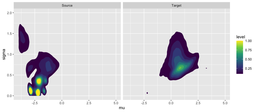
(a) Distribution of (left) source and (right) target data

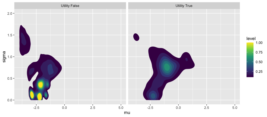
(b) Distribution of source when (left) $U=0$ and (right) $U=1$

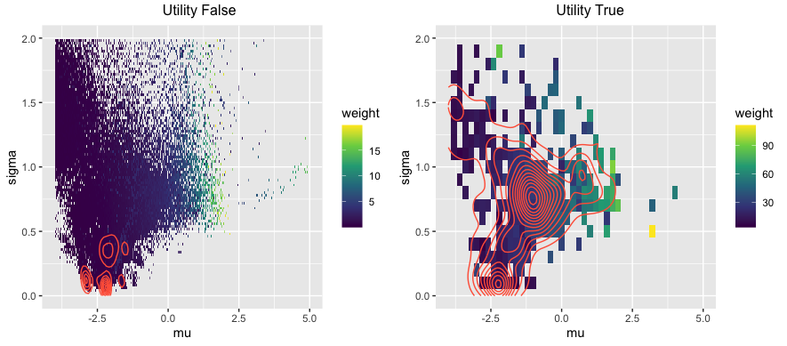
(c) Weights fitted for source dataset where (left) $U=0$ and (right) $U=1$

Figure 3: Landscape of distribution shift in RTB dataset: (Top) Distribution of source and target dataset (Middle) Distribution of source dataset conditioned on utility (Bottom) Distribution of weights fitted on source dataset.

In this section, we proceed with model fitting using the Algorithm 1 based on data that has been created to closely resemble actual RTB bid records. The rationale for the existence of selection bias in RTB market data is as follows. In the RTB context, $U$ is only observable when an auction is won. This restricts our source dataset spectrum; we cannot train for all incoming bid opportunities and features to optimize the utility prediction model. Instead, our training is limited to the subset where we have won the auction. Meanwhile, we desire to estimate the expected utility $\operatorname*{\mathbb{E}}U$ for all bid opportunities. As a result, we aim to learn the classification trained on the winning bid set to perform a new task: estimating distribution of utilities on the total bid set.

To proceed with the modeling, we first train the model for estimating $p:=\operatorname*{\mathbb{P}}(U|X,\text{win})$ given a feature set $X$ via deep neural network (DNN) using all possible feature sets. Here, $\operatorname*{\hat{\eta}}_{W}$ in the algorithm corresponds to $\operatorname*{\hat{\eta}}_{W,0}(X)=1-p,\ \operatorname*{\hat{\eta}}_{W,1}(X)=p$. Then, we select sufficient statistics to use, here we selected 20 variables trained from the user and market features. Among them, the estimated mean($\hat{\mu}(X)$) and variance($\hat{\sigma}(X)$) of the market condition is extracted through fitting DNN models based on all feature sets. To meet the conditions outlined in Lemma 2, if a categorical variable is used in $T(X)$, there should be ample samples to guarantee the presence of anchor set elements for every category.

Figure 3 displays the nature of the distribution shift within the simulated RTB dataset. Within subplots (a) and (b), colors denote the levels of joint density, while in subplot (c), colors reflect the fitted weight values. In Figure 3 (a), the joint distributions of features $m(X)$ and $\sigma(X)$ for both source and target datasets are visualized. It’s evident that the target distribution for $m(X)$ leans slightly more towards the larger values compared to the source distribution. Figure 3 (b) illustrates the distributions of the source dataset when conditioned on utility values, specifically $U=0$ and $U=1$. It’s noticeable that when utility is present, the distribution tends to have a larger mean compared to when it’s absent. Finally, Figure 3 (c) presents the fitted weight values we obtained after applying ExTRA algorithm, alongside the contour of the joint density in red lines. The fitted weights are applied to the source dataset, ensuring that the weighted distribution aligns closely with the target distribution. Since weights are assigned conditionally on utility, even in the presence of class imbalance, the minor distribution is not neglected. Furthermore, as an adaptive response to the observed distribution shifts, we found that the weights show a clear inclination towards regions with larger means.

5 Conclusion

In this paper, we explore the binary classification challenge in the Real-Time Bidding (RTB) market, with a primary focus on the distribution shifts caused by selection bias. To address this, we introduced the exponential tilt model as a way to estimate weights between the source and target domains, expecting it could enhance the model’s potential to perform effectively in a newly targeted domains.

Yet, to truly justify the use and ascertain the efficacy of this method, more thorough examinations and simulations are essential. Especially simulations considering scenarios outlined in eq (5) should be further applied. Specifically, by setting the selection mechanism based on a class-conditional function of X, it’s crucial to understand and explore how the choice of $T(X)$ impacts the performance of re-weighting. By delving into such problems, we need to evaluate the model’s effectiveness when the sufficient statistic is misspecified in real-world scenarios, and how adeptly our reweighting method can account for distribution shifts inherent in selection bias. We earmark these areas for further research.

Having tested the exponential tilting method in the context of the RTB market, we aspire to see if it can be a valuable tool for managing distribution shifts across various machine learning scenarios.

References

- (1)
- Fernando & Tsokos (2022) Fernando, K. R. M. & Tsokos, C. P. (2022), ‘Dynamically weighted balanced loss: Class imbalanced learning and confidence calibration of deep neural networks’, IEEE Transactions on Neural Networks and Learning Systems 33(7), 2940–2951.
- Goodfellow et al. (2015) Goodfellow, I. J., Shlens, J. & Szegedy, C. (2015), Explaining and harnessing adversarial examples, in ‘International Conference on Learning Representations, ICLR’.
- Hendrycks & Dietterich (2019) Hendrycks, D. & Dietterich, T. (2019), Benchmarking neural network robustness to common corruptions and perturbations, in ‘International Conference on Learning Representations, ICLR’.
- Li et al. (2021) Li, T., Beirami, A., Sanjabi, M. & Smith, V. (2021), Tilted empirical risk minimization, in ‘International Conference on Learning Representations, ICLR’.
- Maity et al. (2020) Maity, S., Sun, Y. & Banerjee, M. (2020), ‘Minimax optimal approaches to the label shift problem in non-parametric settings’, J. Mach. Learn. Res. 23, 346:1–346:45.
- Maity et al. (2023) Maity, S., Yurochkin, M., Banerjee, M. & Sun, Y. (2023), Understanding new tasks through the lens of training data via exponential tilting, in ‘International Conference on Learning Representations, ICLR’.
- Osband et al. (2016) Osband, I., Blundell, C., Pritzel, A. & Van Roy, B. (2016), Deep exploration via bootstrapped dqn, in D. Lee, M. Sugiyama, U. Luxburg, I. Guyon & R. Garnett, eds, ‘Advances in Neural Information Processing Systems’, Vol. 29, Curran Associates, Inc.
- Pozzolo et al. (2015) Pozzolo, A. D., Caelen, O., Johnson, R. A. & Bontempi, G. (2015), Calibrating probability with undersampling for unbalanced classification, in ‘2015 IEEE Symposium Series on Computational Intelligence’, pp. 159–166.
- Quionero-Candela et al. (2009) Quionero-Candela, J., Sugiyama, M., Schwaighofer, A. & Lawrence, N. D. (2009), Dataset Shift in Machine Learning, The MIT Press.
- Shimodaira (2000) Shimodaira, H. (2000), ‘Improving predictive inference under covariate shift by weighting the log-likelihood function’, Journal of Statistical Planning and Inference 90(2), 227–244.
- Wallace & Dahabreh (2013) Wallace, B. & Dahabreh, I. (2013), ‘Improving class probability estimates for imbalanced data’, Knowledge and Information Systems 41.
- Zhang et al. (2021) Zhang, A., Lipton, Z. C., Li, M. & Smola, A. J. (2021), ‘Dive into deep learning’, arXiv preprint arXiv:2106.11342 .