Online Class Cover Problem

Abstract

In this paper, we study the online class cover problem where a (finite or infinite) family $\cal F$ of geometric objects and a set ${\cal P}_{r}$ of red points in $\mathbb{R}^{d}$ are given a prior, and blue points from $\mathbb{R}^{d}$ arrives one after another. Upon the arrival of a blue point, the online algorithm must make an irreversible decision to cover it with objects from $\cal F$ that do not cover any points of ${\cal P}_{r}$. The objective of the problem is to place the minimum number of objects. When $\cal F$ consists of all possible translates of a square in $\mathbb{R}^{2}$, we prove that the competitive ratio of any deterministic online algorithm is $\Omega(\log|{\cal P}_{r}|)$. On the other hand, when the objects are all possible translates of a rectangle in $\mathbb{R}^{2}$, we propose an $O(\log|{\cal P}_{r}|)$-competitive deterministic algorithm for the problem.

Keywords: Class Cover, Online Algorithm, Squares, Translated Objects, Competitive Ratio.

1 Introduction

Let ${\cal P}_{b}$ and ${\cal P}_{r}$ be two sets of blue and red points in $\mathbb{R}^{d}$, where $|{\cal P}_{b}|=n$ and $|{\cal P}_{r}|=m$. In this scenario, the set ${\cal P}={\cal P}_{b}\cup{\cal P}_{r}$ is called a bi-coloured point set, and ${\cal P}_{b}$ and ${\cal P}_{r}$ are referred to as the blue and red point classes, respectively. A geometric object (for example, ball, hypercube etc.) is considered ${\cal P}_{r}$-empty if it does not contain any point from the set ${\cal P}_{r}$. For a given (finite or infinite) family $\cal F$ of geometric objects in $\mathbb{R}^{d}$ and a bi-coloured set ${\cal P}={\cal P}_{b}\cup{\cal P}_{r}$, the objective of the class cover problem is to find a minimum cardinality subset $\cal S\subseteq\cal F$, consisting of only ${\cal P}_{r}$-empty geometric objects, that covers the blue point class (i.e., every point in ${\cal P}_{b}$ is contained in at least one of the objects without covering any points in ${\cal P}_{r}$).

For our research, we are considering the online class cover problem where we only know the red point class ${\cal P}_{r}$ and don’t know the blue point class in advance. The blue points will come one by one, and upon the arrival of a blue point, we need to make an irreversible decision to cover it with ${\cal P}_{r}$-empty objects. Again, the objective of the problem is to find a minimum cardinality set of ${\cal P}_{r}$-empty objects. In this paper, we consider the problem when $\cal F$ is the set of all translated copies of a rectangle in $\mathbb{R}^{2}$, and ${\cal P}_{r}$ is a set of points in $\mathbb{R}^{2}$.

The quality of the online algorithm is analyzed using competitive analysis [5]. The competitive ratio of an online algorithm is $\sup_{{\cal I}}\left(\frac{\text{ALG}({\cal I})}{\text{OPT}({\cal I})}\right)$, where ${\cal I}$ is an input sequence, and $\text{OPT}({\cal I})$ and $\text{ALG}({\cal I})$ are the cost of an optimal offline algorithm and the solution produced by the online algorithm, respectively, over ${\cal I}$. Here, the supremum is taken over all possible input sequences ${\cal I}$.

Online computation models capture many real-world phenomena: the irreversibility of time (decisions), the inaccessibility of complete data, and the ambiguity of the future. As a result, online models of computation have attracted many researchers. In computational geometry, much work has been conducted on the online model for various problems such as the set cover problem [11, 19, 20], hitting set problem [17, 22, 24], independent set problem [8, 23], coloring problem [12, 13] and the dominating set problem [16, 21]. There is a lack of literature on the online class cover problem. This is a natural problem, and it has various applications in data mining, pattern recognition, scientific computation, visualization and computer graphics [1, 18, 25]. An application example of the online class cover problem inspired by Alon et al. [2] is as follows. Consider, for instance, network servers that provide a service. A set of clients may require the service, and each server can provide it to a subset of those clients. The requests of clients arrive one by one. The network administrator must determine where to deploy a server upon the introduction of a client so that the client receives the requested service. However, there may be some customers who utilise the services of a competitor. Therefore, the network administrator must install the server to exclude rival clients and cover the area where a potential future client may arrive.

1.1 Related Work

We aren’t aware of any work in the online setting of the class cover problem. But in the offline setting, some of the key results are highlighted below. Inspired by the Cowen–Priebe method for the classification of high-dimensional data (see [7, 14]), Cannon and Cowen [6] introduced the class cover problem as follows:

Minimize $$k$$

Subject to, $$\max_{u\in{\cal P}_{b}}d(u,S)\leq\min_{u\in{\cal P}_{r}}d(u,S),$$

$$\text{where}\ S\subseteq{\cal P}_{b},|S|=k.$$

Here the point-to-set distance $d(u,S)$ is defined as $\min_{s\in S}d(u,s)$. In other words, given a bi-coloured set ${\cal P}={\cal P}_{b}\cup{\cal P}_{r}$, the objective is to find a minimum cardinality set of blue centers to cover the blue points with a set of blue-centered balls of equal radius, such that no red points lie in these balls. They showed that this problem is NP-hard and gave an $(1+\ln|{\cal P}|)$-approximation algorithm for general metric spaces that runs in cubic time. They presented a polynomial-time approximation scheme (PTAS) in the Euclidean setting for constant dimension.

In [4], Bereg et al. considered the class cover problem for axis-aligned rectangles (i.e. boxes) and called it the Boxes Class Cover problem (BCC problem). They proved the NP-hardness of the problem and gave an $O(\log|\text{OPT}|)$-approximation algorithm, where OPT is an optimal covering. They also study some variants of the problem. If the geometric objects are axis-parallel strips and half-strips oriented in the same direction, they gave an exact algorithm running in $O(m\log m+n\log n+\sqrt{mn})$-time and $O((m+n)\log(\min\{m,n\}))$-time, respectively. However, if half-strips are oriented in any of the four possible orientations, the problem is NP-hard. But in this case, they showed that there exists an $O(1)$-approximation algorithm. In the last variant of the BCC problem, they considered axis-aligned squares. Here, they proved the NP-hardness of the problem and presented an $O(1)$-approximation algorithm. Shanjani [26] proved that the BCC problem is APX-hard, whereas a PTAS exists for the variant of the problem for disks and axis-parallel squares [3].

In [9], Cardinal et al. considered a symmetric version of the BCC problem and called it Simultaneous BCC problem (SBCC problem), which is defined as follows: Given a set ${\cal P}$ of points in the plane, each coloured red or blue, find the smallest cardinality set of axis-aligned boxes which together cover ${\cal P}$ such that each box cover only points of the same colour and no box covering a red point intersects the interior of a box covering a blue point [9, Dfn. 2]. They showed that this problem is APX-hard and gave a constant-factor approximation algorithm.

If the red point class ${\cal P}_{r}$ is empty, and $\cal F$ consists of all possible translated copies of an object, then the online class cover problem is equivalent to the online unit cover problem. Charikar et al. [11] proposed an $O(2^{d}d\log d)$ competitive algorithm for the online unit cover for balls in $\mathbb{R}^{d}$. Later, Dumitrescu et al. [19] obtained $O({1.321}^{d})$ competitive algorithm and proved that the lower bound is $\Omega(d+1)$. In particular, for balls in $\mathbb{R}^{2}$ and $\mathbb{R}^{3}$, they obtained competitive ratios of 5 and 12, respectively. Dumitrescu and Tóth [20] studied the unit cover problem for hyper-cubes in $\mathbb{R}^{d}$. They proved that the lower bound of this problem is at least $2^{d}$, and also this ratio is optimal, as it is obtainable through a simple deterministic algorithm that allocates points to a predefined set of hyper-cubes [10]. Recently, De et al. [15] gave a deterministic online algorithm of the unit cover problem for $\alpha$-aspect_∞ objects in $\mathbb{R}^{d}$ with competitive ratio at most $\left(\frac{2}{\alpha}\right)^{d}((1+\alpha)^{d}-1)\log_{(1+\alpha)}\left(\frac{2}{\alpha}\right)+1$. To summarise existing results related to the online unit cover problem using translates of an object of various shapes, we refer to Table 1 of [ibid.]

Consider the online class cover problem when $\cal F$ is an infinite family of intervals on $\mathbb{R}$ and ${\cal P}_{r}$ is a set of $m$ red points in $\mathbb{R}$. Observe that the $m$ red points partition $\mathbb{R}$ into $m+1$ open intervals. As a result of this, any ${\cal P}_{r}$-empty interval must lie inside one of the $m+1$ open intervals. Therefore, the online class cover problem for intervals in $\mathbb{R}$ reduces to $m+1$ distinct online set cover problems for intervals in $\mathbb{R}$. For this case, if $\cal F$ is the set of all possible translations of an interval, then an optimum $2$-competitive algorithm for the problem can be obtained [10, 11].

1.2 Our Contributions

This paper primarily presents two results on the online class cover problem when $\cal F$ is the set of all possible axis-parallel unit squares in $\mathbb{R}^{2}$, and ${\cal P}_{r}$ is a set of points in $\mathbb{R}^{2}$. We show, first, that the competitive ratio of every deterministic online algorithm of the problem is $\Omega(\log m)$ (Theorem 1). To prove this, we consider an adaptive adversary. Initially, the adversary constructs a set ${\cal P}_{r}$ of $m$ red points such that a unit square contains ${\cal P}_{r}$. In each of $O(\log m)$ rounds, the adversary maintains a subset $P\subseteq{\cal P}_{r}$ of red points and places a blue point in a grid cell, obtained by using the points in $P$, such that any online algorithm must place a new square to cover it, whereas an offline optimal covers all the blue points by a single square.

Next, we provide a deterministic online algorithm with a competitive ratio of $O(\log m)$ (Theorem 2 and Theorem 3). Our algorithm, in a nutshell, is as follows: when a new blue point is introduced to the algorithm that is uncovered by the previously selected squares, the algorithm chooses at most five squares, called candidate squares (see Section 4.3 for definition), to cover it. The candidate squares are constructed using a binary search over potential squares. The main challenge and the novelty is to show that the candidate squares are sufficient to establish the competitive ratio. As stated previously, the online class cover problem reduces to the online unit cover problem if ${\cal P}_{r}=\emptyset$, and in that case for squares, note that our algorithm achieves the known optimal competitive ratio of 4 [10, 20]. Furthermore, we show that the same upper bound of the online class cover problem applies to translated copies of a rectangle (Theorem 4).

1.3 Outline of the Paper

In Section 2, we introduce terminology that will be used in subsequent sections. Section 3 demonstrates the lower bound for the online class cover problem for axis-parallel unit squares. Then, in Section 4, we present an online algorithm of the problem. In Section 5, we give our algorithm’s correctness and competitive analysis. In Section 6, we examine the online class cover problem for translated copies of a rectangle. Finally, we conclude in Section 7.

2 Notation and Preliminaries

(a)

(b)

(c)

Figure 1: (a) An axis-parallel unit square $R(u)=\square abcd$ centered at $u$. (b) The square $R(u+\tau_{x})$ (red) is a horizontal translated copy of $R(u)$ (black). (c) An $8\times 8$ gird ${\cal G}(Q)$ using $9$ points of $Q=\{u_{1},u_{2},\dots,u_{9}\}$ in a plane.

We use $[n]$ to represent the set $\{1,2,\ldots,n\}$. We use the phrase ‘$X$ contains $Y$’ to signify that $Y\subseteq X$. For any point $u$, we use $u(x)$ and $u(y)$ to denote the $x$ and $y$-coordinates of $u$, respectively. A point $u$ is said to be lying on the left side of a vertical line segment $l$ if $u$ lies on the left side of the line $L$, obtained by extending the line segment $l$ in both directions. Similarly, we define the other cases such as $u$ lying on the right, the above and the bottom side of a horizontal/vertical line segment $l$. Let $R(u)=\square abcd$ be an axis-parallel unit square centred at a point $u$ (see Figure 1(a)). Let $p,q,r$ and $s$ be the midpoints of the edges $ab,bc,cd$ and $ad$ of $R(u)$, respectively. The vertices $a,b,c$ and $d$ will be called $NW,SW,SE$ and $NE$ vertices of $R(u)$, respectively. The edges $ab,bc,cd$ and $ad$ will be called the left, the bottom, the right and the top edge of $R(u)$, respectively. Now the two line segments $\overline{pr}$ and $\overline{qs}$ partition $R(u)$ into four sub-squares $R(u)_{NW}=\square apus,R(u)_{SW}=\square pbqu,R(u)_{SE}=\square uqcr$ and $R(u)_{NE}=\square surd$ each of side length $\frac{1}{2}$. The boundary of $R(u)$ will be denoted by $\partial R(u)$, and the interior by $\operatorname{int}(R(u))=\{v\in R(u)\ |\ v\notin\partial R(u)\}$. A point $v$ is said to be covered/contained by a square $R(u)$ if $v\in\operatorname{int}{(R(u))}$. Throughout the paper, a square means an axis-parallel unit square unless mentioned.

Let $\tau_{xy}=(x,y)$ be a vector in $\mathbb{R}^{2}$. We denote $\tau_{x0}=(x,0)$ and $\tau_{0y}=(0,y)$ as $\tau_{x}$ and $\tau_{y}$, respectively. A translated copy of $R(u)$ is a square $P$ such that $P=R(u+\tau_{xy})=\{v+\tau_{xy}\ |\ v\in R(u)\}$. We say that a square $P$ is a horizontal translated copy of $R(u)$ if $P=R(u+\tau_{x})$ (see Figure 1(b)). Similarly, $P=R(u+\tau_{y})$ is said to be a vertical translated copy of $R(u)$. A square $R(u)$ is moved rightwards, meaning that we always consider a horizontal translated copy $R(u+\tau_{x})$ of $R(u)$ by continuously increasing $x$ in the positive direction. Similarly, we can define the movement of $R(u)$ in other directions, such as leftwards, upwards and downwards.

Let $Q=\{u_{1},u_{2},\dots,u_{q}\}$ be a set of points in a plane having distinct $x$ and $y$-coordinates. Consider the horizontal and vertical lines passing through each point $u\in Q$. They form a $(q-1)\times(q-1)$ grid, denoted by ${\cal G}(Q)$ (see Figure 1(c)). We consider the bottom-most row of ${\cal G}(Q)$ as $1$st row and the right-most column of ${\cal G}(Q)$ as $1$st column. Let $G_{ij}$ be the cell in the grid that appears in the $i$th row and the $j$th column for $i,j\in[q-1]$. Note that $G_{11}$ and $G_{(q-1)(q-1)}$ are the $SE$ and the $NW$ corner cells in the grid. A grid cell $G_{ij}$ is said to be cover-free with respect to a set $\{R_{1},\dots,R_{k}\}$ of squares, if there exists a point $v\in G_{ij}$ such that $v\notin\left(\cup_{i=1}^{k}R_{i}\right)$.

For any two points $a,b\in\mathbb{R}^{2}$, we use $d(a,b)$ to represent the distance between the points $a$ and $b$ under the Euclidean norm. Let $L$ be any horizontal or vertical line. Define, $d(a,L)=\min_{u\in L}d(a,u)$. Consider a set $Q$ of points. Now a point $u\in Q$ is said to be the nearest point to the line $L$, if $d(u,L)=\min_{a\in Q}d(a,L)$ (see Figure 2(a)). With slight abuse, a point $v\in Q$ is said to be the nearest point to a line segment $l$ if $v$ is the nearest point to the line $L$, obtained by extending the line segment $l$ in both directions.

(a)

(b)

(c)

Figure 2: (a) The point $u_{2}\in Q$ is nearest to the line $L$, where $Q=\{u_{1},u_{2},\dots,u_{6}\}$. (b) Here, $ST_{SW}(Q)$ is the sequence $\sigma=\{l_{1},h_{1},\dots,$ $l_{4},h_{4}\}$, where $Q=\{u_{1},u_{2},\dots,u_{5}\}$. (c) The square $P(u+\tau_{xy})$ (red) is obtained by moving $R(u)$ (black) rightwards along the staircase.

For a set $Q$ of points, define the set $D_{SW}(Q)=\{q\in Q\ |\ \nexists\ q^{\prime}\in Q$ such that $q(x)<q^{\prime}(x)$ and $q(y)<q^{\prime}(y)\}$. We call $D_{SW}(Q)$ the set of $SW$ dominating point of $Q$. Similarly, we can define the other dominating sets of $Q$ such as $D_{NW}(Q),D_{NE}(Q)$ and $D_{SE}(Q)$. Let $Q^{\prime}=D_{SW}(Q)=\{u_{1},u_{2},\dots,u_{q}\}$ be such that $u_{i}(x)\leq u_{i+1}(x)$ and $u_{i}(y)\geq u_{i+1}(y)$ for $i\in[q-1]$. Now, we define a SW staircase of $Q$, denoted by $ST_{SW}(Q)$, as an alternating sequence $\{l_{1},h_{1},\dots,$ $l_{q-1},h_{q-1}\}$ of vertical and horizontal line segments such that $l_{i}=\overline{u_{i}u^{\prime}_{i}}$ and $h_{i}=\overline{u^{\prime}_{i}u_{i+1}}$, where $u^{\prime}_{i}=(u_{i}(x),u_{i+1}(y))\in\mathbb{R}^{2}$ for $i\in[q-1]$ (see Figure 2(b)). The two points $u_{1}$ and $u_{q}$ are called the initial point and the terminal point of $ST_{SW}(Q)$, respectively. Similarly, we can define the other staircases of $Q$ such as $ST_{NW}(Q)$, $ST_{NE}(Q)$ and $ST_{SE}(Q)$. Let $R(u)$ be a square such that the $SW$ vertex of $R(u)$ coincide with $u^{\prime}_{i}$ for some $i\in[q]$. Now, $R(u)$ is moved rightwards along the staircase $ST_{SW}(Q)$ means that we always consider a translated copy $P=R(u+\tau_{xy})$ of $R(u)$ such that the $SW$ vertex of $P$ always lies either on $l_{j}$ or on $h_{j}$ for some $j\in[q-1]$ by continuously increasing either $x$ in the positive direction or $y$ in the negative direction (see Figure 2(c)). Similarly, we can define the movement of $R(u)$ along the staircase $ST_{SW}(Q)$ in the leftward direction.

3 Lower Bound Construction

In this section, we present a lower bound of the online class cover problem for squares.

Theorem 1.

The competitive ratio of every deterministic online algorithm for the class cover problem for squares is at least $\max\{4,\lfloor\log_{2}m\rfloor+1\}$, where $m\ (\geq 0)$ is the number of red points.

(a)

(b)

Figure 3: Example of the lower bound of the online class cover problem using axis-parallel unit square where $m=9$. (a) To cover $b_{1}$, the algorithm places the square $R_{1}$ (blue), and $O_{1}$ is the red-coloured square. (b) To cover $b_{2}$, the algorithm places the square $R_{2}$ (green), and $O_{2}$ is the red-coloured square that covers both $b_{1}$ and $b_{2}$.

Proof.

Dumitrescu and Tóth [20] proved that the competitive ratio of every deterministic online algorithm for the set cover problem using axis-parallel unit squares in a plane is at least $4$. This lower bound applies to the online class cover problem for $m\geq 0$. To prove the theorem, we construct a lower bound $\lfloor\log_{2}m\rfloor+1$ of the problem for $m\geq 8$.

Let ${\cal P}_{r}=\{r_{1},r_{2},\dots,r_{m}\}$ be a set of $m\ (\geq 8)$ red points in a plane lying on the line $x=y$ such that the distance between $r_{1}$ and $r_{m}$ is $\sqrt{2}$, and $r_{i}(x)<r_{i+1}(x)$ for $i\in[m-1]$. For simplicity, let us assume that $m=2^{p}$ for some integer $p$. To prove the lower bound, we construct an input sequence of $p+1$ many blue points $b_{1},b_{2},\dots,b_{p+1}\in{\cal P}_{b}$ using an adaptive adversary; for which an offline optimal algorithm needs just one square, whereas any online algorithm needs at least $p+1$ many squares to cover them without containing any red points. See Figure 3 for an example when $m=9$. For each $i\in[p+1]$, the adversary maintains a set ${\cal P}_{r}^{(i)}\subseteq{\cal P}_{r}$, and places the blue point $b_{i}$ inside a cell $C_{i}$ of the grid ${\cal G}({\cal P}_{r}^{(i)})$. Let $O_{i}$ be a square whose left and top edges coincide with the left and top edges of $C_{i}$, respectively. We set ${\cal P}_{r}^{(0)}={\cal P}_{r}$ and $O_{0}=\emptyset$. For each $i\in[p+1]$, let $R_{i}$ be a square, placed by an online algorithm in $i$th iteration to cover $b_{i}$ and $R_{0}=\emptyset$. We construct the sequence $\{b_{1},b_{2},\dots,b_{p+1}\}$ inductively so that the following invariants will always be satisfied for $i=1,2,\dots,p+1$.

• ${\cal P}_{r}^{(i)}\subseteq{\cal P}_{r}^{(i-1)}$ and $|{\cal P}_{r}^{(i)}|\geq\frac{m}{2^{i-1}}$.

• Each grid cell of ${\cal G}({\cal P}_{r}^{(i)})$ is cover-free with respect to the set $\{R_{0},R_{1},\dots,R_{i-1}\}$ of squares.

• The blue point $b_{i}$ is placed inside the $SE$ corner cell, say $C_{i}$, of the grid ${\cal G}({\cal P}_{r}^{(i)})$ such that $b_{i}\notin\left(\cup_{j=0}^{i-1}R_{j}\right)$.

• All blue points $b_{1},\dots,b_{i}$ are covered by the square $O_{i}$ that contains no red points.

In the first iteration, we consider ${\cal P}_{r}^{(1)}={\cal P}_{r}$, and it is easy to see that invariant (1) holds. Now the adversary places the blue point $b_{1}$ inside the $SE$ corner grid cell, say $C_{1}$, of ${\cal G}({\cal P}_{r}^{(1)})$. Thus invariants (2) and (3) hold. Here, the square $O_{1}$ contains $b_{1}$. Therefore, invariant (4) also holds.

Let us assume that all the invariants hold for $i=1,2,\dots,k$ (where, $k\leq p$). Now we will prove that the invariants hold for $i=k+1$. Let $a$ be the $NW$ vertex of $R_{k}$. If $a$ does not lie on any grid edge, then it lies inside a cell of ${\cal G}({\cal P}_{r}^{(k)})$. Let $G_{uv}$ be that cell. Otherwise, we define $u$ and $v$ as follows: $u=\max\{i\in[m-1]\ |\ a\in G_{ij}\}$ and $v=\max\{j\in[m-1]\ |\ a\in G_{ij}\}$. Suppose $v_{k}$ (resp., $h_{k}$) is the vertical line (resp., horizontal line) passing through the right edge (resp., bottom edge) of $G_{uv}$ (see Figure 4). Let $V_{k}$ (resp., $H_{k}$) be the half-plane lying on the left side (resp., top side) of the line $v_{k}$ (resp., $h_{k}$). Now, the adversary considers two subset ${\cal R}_{V}$ and ${\cal R}_{H}$ of ${\cal P}_{r}^{(k)}$ as follows: ${\cal R}_{V}=\{r_{i}\in{\cal P}_{r}^{(k)}\ |\ r_{i}$ lies on the half-plane $V_{k}\}$, and ${\cal R}_{H}=\{r_{i}\in{\cal P}_{r}^{(k)}\ |\ r_{i}$ lies on the half-plane $H_{k}\}$.

• 

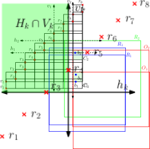
  Figure 4: Here, ${\cal R}_{V}=\{r_{1},r_{2},r_{3},r_{4}\}$ and ${\cal R}_{H}=\{r_{3},r_{4},r_{5},r_{6},r_{7},r_{8}\}$. The green shaded region denotes the common region of the two half-planes $H_{k}$ and $V_{k}$. Also, ${\cal R}_{V}\cup{\cal R}_{H}={\cal P}_{r}^{(k)}=\{r_{1},r_{2},\dots,r_{8}\}$.

• Let ${\cal P}_{r}^{(k+1)}$ be the set among ${\cal R}_{V}$ and ${\cal R}_{H}$ with the maximum size. Since $R_{k}$ contains no red points, the $NW$ vertex $a$ of $R_{k}$ must lie in $V_{k}\cap H_{k}$, i.e. $a\in V_{k}\cap H_{k}$. As a result, we have that for each $r\in{\cal P}_{r}^{(k)}$, either $r\in{\cal R}_{V}$ or $r\in{\cal R}_{H}$. Therefore, ${\cal R}_{V}\cup{\cal R}_{H}={\cal P}_{r}^{(k)}$ (see Figure 4). Hence, either $|{\cal R}_{V}|\geq\frac{{\cal P}_{r}^{(k)}}{2}$ or $|{\cal R}_{H}|\geq\frac{{\cal P}_{r}^{(k)}}{2}$. This implies that $|{\cal P}_{r}^{(k+1)}|\geq\frac{{\cal P}_{r}^{(k)}}{2}\geq\frac{m}{2^{k}}$, and invariant (1) holds.

• Since ${\cal P}_{r}^{(k+1)}\subseteq{\cal P}_{r}^{k}$ and each grid cell of ${\cal G}({\cal P}_{r}^{(k)})$ is cover-free with respect to the set $\{R_{1},R_{2},\dots,$ $R_{k-1}\}$, each of the grid cell of ${\cal G}({\cal P}_{r}^{(k+1)})$ is also cover-free with respect to $\{R_{1},R_{2},\dots,R_{k-1}\}$. Now from the construction of ${\cal P}_{r}^{(k+1)}$, we can see that if ${\cal P}_{r}^{(k+1)}={\cal R}_{V}$ (resp., ${\cal P}_{r}^{(k+1)}={\cal R}_{H}$), then all the cell $G_{uj}$ for $j\in[v]$ (resp., $G_{iv}$ for $i\in[u]$) are the only cells of the grid ${\cal G}({\cal P}_{r}^{(k+1)})$ that may have some non-empty intersection with $R_{k}$. But each of the cell $G_{uj}$ (resp., $G_{iv}$) is cover-free with respect to the set $\{R_{k}\}$. As a result, each cell of the grid ${\cal G}({\cal P}_{r}^{(k+1)})$ is cover-free with respect to $\{R_{k}\}$. Therefore, invariant (2) holds.

• Due to invariant (2), a blue point $b_{k+1}$ can be placed inside the $SE$ corner cell, say $C_{k+1}$, of the grid ${\cal G}({\cal P}_{r}^{(k+1)})$ such that $b_{k+1}\notin\left(\cup_{j=0}^{k}R_{j}\right)$. Therefore, invariant (3) holds.

• Since $O_{k+1}$ covers $C_{k+1}$, we have, $b_{k+1}\in O_{k+1}$. Observe that if ${\cal P}_{r}^{(k+1)}={\cal R}_{V}$ (resp., ${\cal P}_{r}^{(k+1)}={\cal R}_{H}$), then $C_{k}$ and $C_{k+1}$ will be in the same column (resp., row) of the grid ${\cal G}({\cal P}_{r}^{(k)})$. Also, note that the height of the grid ${\cal G}({\cal P}_{r}^{(k)})$ is at most $1$. As a result of this, we have, $O_{k}\cap{\cal G}({\cal P}_{r})\subseteq O_{k+1}\cap{\cal G}({\cal P}_{r})$. Thus, $O_{k+1}$ also contains $b_{1},\dots,b_{k}$. Therefore, invariant (4) holds.

Hence all the invariants also hold for $i=k+1$. Therefore, the theorem follows. ∎

4 An Online Algorithm

In this section, we present an online algorithm for the class cover problem for the translates of a square. If a blue point $u$, introduced to the algorithm, is already covered by previously selected squares, the algorithm doesn’t introduce additional squares in this step. Otherwise, we define at most five squares, called the candidate squares, ${\mathcal{S}}(u)=\{R_{1},R_{2},R_{3},R_{4},R_{5}\}$ for the point $u$ as given in Section 4.3, and our algorithm places each of these candidate squares to cover the point $u$. Though any of the candidate squares is sufficient to cover $u$, we need all the candidate squares to derive the bound on the competitive ratio. Before illustrating the set of candidate squares, we demonstrate an important notion of the set of possible candidate squares, for a blue point $u$ in Section 4.1. Then we illustrate how to construct three candidate squares $R_{1},R_{2}$ and $R_{3}$ from a set of possible candidate squares in Section 4.2. Later on, using this tool, we demonstrate how to obtain all five candidate squares in Section 4.3. In Section 4.4, we formally describe our algorithm. Moreover, we characterize the candidate squares in two types, Type 1 and Type 2, depending on whether it is constructed by using the set of possible candidate squares or not. We will construct the candidate squares so that $R_{1},R_{2}$ and $R_{3}$ are always Type 1 candidate squares, and $R_{4}$ and $R_{5}$ are always Type 2 candidate squares.

Let $u$ be a blue point, and $R(u)=\square abcd$ be the square centred at $u$. Let $R(u)_{NW}=\square apus,$$R(u)_{SW}=\square pbqu,$ $R(u)_{SE}=\square uqcr$ and $R(u)_{NE}=\square surd$ be the four sub-squares of $R(u)$ (as defined in Section 2). The construction of the candidate squares solely relies on the following observation.

Observation 1.

Let $u$ be any blue point and $P$ be any square such that $u\in P$. Then, $P$ must contain at least one sub-square of $R(u)$.

4.1 Possible Candidate Squares

Consider a blue point $u$ and the square $R(u)$ centered at it. Suppose that $R(u)_{SW}$ contains some red points, but $R(u)_{NE}$ is red point free. Now, if $R(u)_{NW}\cap{\cal P}_{r}\neq\emptyset$, let $r_{1}\in R(u)_{NW}\cap{\cal P}_{r}$ be a red point nearest to the line segments $\overline{us}$; otherwise, let $r_{1}=a$, and if $R(u)_{SE}\cap{\cal P}_{r}\neq\emptyset$, let $r_{2}\in R(u)_{SE}\cap{\cal P}_{r}$ be a red point nearest to the line segments $\overline{ur}$; otherwise, let $r_{2}=c$. Let $R^{\prime}$ be a square whose left edge and bottom edge pass through the points $r_{1}$ and $r_{2}$, respectively (see Figure 5(a)).

(a)

(b)

Figure 5: $R(u)$ (black) is the square centered at the blue point $u$. (a) The set of $SW$ staircase points ${\cal Q}(u)_{SW}=\{r_{1},q_{0},\dots,q_{3},r_{2}\}$ forms the staircase $ST_{SW}({\cal Q}(u)_{SW})$ (dark green), and $P_{0},P_{2},P_{4}$ (blue) are some possible candidate squares of $u$. Also, $u\in P_{0},P_{2},P_{4}$. (b) Case 1.1: $R^{\prime}_{SW}$ contains no red points. Here, $R_{4}$ is a candidate square (blue) of $u$ obtained by moving $R^{\prime}$ (black/dashed).

Let $Q^{\prime}=R(u)_{SW}\cap R^{\prime}_{SW}\cap{\cal P}_{r}$, and $Q^{\prime\prime}=D_{SW}(Q^{\prime})$, the set of $SW$ dominating point of $Q^{\prime}$. Now, consider $Q^{\prime\prime}=\{q_{0},q_{1},\dots,q_{k}\}$ such that $q_{i}(x)\leq q_{i+1}(x)$ and $q_{i}(y)\geq q_{i+1}(y)$ for all $i\in\{0\}\cup[k-1]$. The set ${\cal Q}(u)_{SW}=\{r_{1},q_{0},q_{1},\dots,q_{k},r_{2}\}$ will be called the set of $SW$ staircase points of $u$, and it forms a staircase $ST_{SW}({\cal Q}(u)_{SW})$ (see Figure 5(a)). Here, the two points $r_{1}$ and $r_{2}$ are the initial and the terminal point of $ST_{SW}({\cal Q}(u)_{SW})$, respectively.

For each pair of consecutive red points $(q_{j},q_{j+1})$, where $0\leq j\leq k-1$, we have a square $P_{j+1}$ such that $q_{j}$ and $q_{j+1}$ lie on the left and the bottom edge of $P_{j+1}$, respectively. We also define two squares $P_{0}$ and $P_{k+1}$ such that $r_{1}$ and $q_{0}$ lie on the left edge and bottom edge of $P_{0}$, and $q_{k}$ and $r_{2}$ lie on the left edge and bottom edge of $P_{k+1}$, respectively. Now, consider the set $\mathcal{PS}(u)_{SW}=\{P_{j}\ |\ P_{j(NE)}\ \text{contains no red points for}\ j\in\{0\}\cup[k+1]\}$. Let $\mathcal{PS}(u)_{SW}=\{P_{j_{1}},P_{j_{2}},\dots,P_{j_{l}}\}$ such that $\{j_{1},j_{2},\dots,j_{l}\}$ is a sub-sequence of $\{1,2,\dots,k\}$ (see Figure 5(a)). We call $\mathcal{PS}(u)_{SW}$ the set of $SW$ possible candidate squares of $u$ and each square $P_{j_{i}}\in\mathcal{PS}(u)_{SW}$ a possible candidate square of $u$.

Observation 2.

For each $j\in\{0\}\cup[k+1]$, we have $u\in P_{j}$, and the sub-square $P_{j(SW)}$ contains no red points.

Similarly, we can define the other sets such as ${\cal Q}(u)_{NW},\mathcal{PS}(u)_{NW}$ and so on.

Algorithm 1 U(SE)-R(NW)-MOVE$(\langle u,H\rangle)$

1:A blue point $u$, and a translated copy $H$ of $R(u)$ such that $H_{SW}\subseteq R(u)$.

2:A square $P$.

3:while $(H_{NW}\cup H_{SE})$ is not red points free and $H$ contains $u$ do

4:     if $H_{SE}$ contains some red points then

5:         Move $H$ upwards until $H_{SE}$ becomes red points free

6:     end if

7:     if $H_{NW}$ contains some red points then

8:         Move $H$ rightwards until $H_{NW}$ becomes red points free

9:     end if

10:end while

11:if $H$ is red points free and $u\in H$ then

12:     Return $P=H$

13:else

14:     Return $P=\emptyset$

15:end if

4.2 Construction of Type 1 Candidate Squares

In this section, we demonstrate how to obtain Type 1 candidate squares for a blue point $u$ corresponding to a set of possible candidate squares of $u$. W.l.o.g, assume that $R(u)_{SW}$ contains some red points, but $R(u)_{NE}$ is red point free. So, as defined in Section 4.1, consider the set of $SW$ staircase points ${\cal Q}(u)_{SW}=\{r_{1},q_{0},q_{1},\dots,q_{k},r_{2}\}$ and the set of $SW$ possible candidate squares $\mathcal{PS}(u)_{SW}=\{P_{1},P_{2},\dots,P_{l}\}$ of $u$.

If $\mathcal{PS}(u)_{SW}=\emptyset$, then we set $R_{i}=\emptyset$ for $i\in[3]$. W.l.o.g, assume that $\mathcal{PS}(u)_{SW}$ is non-empty. Let $H_{1}=P_{1},H_{2}=P_{\lceil\frac{l}{2}\rceil}$ and $H_{3}=P_{l}$ (they may not be distinct). Note that the way we have defined $H_{i}$ for $i\in[3]$ ensures that $H_{i(SW)}\cup H_{i(NE)}$ does not contain any red point. Now, depending on which sub-squares among $H_{i(SE)}$ and $H_{i(NW)}$ contain red points, we move $H_{i}$ as follows: (1) If $H_{i(SE)}$ and $H_{i(NW)}$ both contain some red point, we set $R_{i}=\text{U(SE)-R(NW)-MOVE}(\langle u,H_{i}\rangle)$ as defined in Algorithm 1.

Algorithm 2 ST-R(NW)-MOVE$(\langle u,H\rangle)$

1:A blue point $u$, and a translated copy $H$ of $R(u)$ such that the $SW$ vertex of $H$ lies on the staircase $ST_{SW}({\cal Q}(u)_{SW})$.

2:A square $P$.

3:if $H_{NW}$ contains some red points then

4:     Move $H$ rightwards along the staircase $ST_{SW}({\cal Q}(u)_{SW})$ until $(H_{NW}\cup H_{NE})$ becomes red points free

5:end if

6:if $H_{SE}$ contains some red points then

7:     Return $P=$U(SE)-R(NW)-MOVE$(\langle u,H\rangle)$

8:     Break

9:else if $H$ is red points free and $u\in H$ then

10:     Return $P=H$

11:else

12:     Return $P=\emptyset$

13:end if

In other words, if $H_{i(NW)}\cup H_{i(SE)}$ contains some red points, first, we move $H_{i}$ upwards until $H_{i(SE)}$ becomes red points free, and then move it rightwards until $H_{i(NW)}$ contains no red points. Repeat the process until $H_{i}$ becomes red points free or does not contain $u$. In the former case, we set $R_{i}=H_{i}$. In the latter case, we set $R_{i}=\emptyset$. (2) Now, consider the case when exactly one of $H_{i(NW)}$ and $H_{i(SE)}$ contains some red points. W.l.o.g., assume that only $H_{i(NW)}$ contains some red points. The other case is similar. In this case, we set $R_{i}=\text{ST-R(NW)-MOVE}(\langle u,H_{i}\rangle)$ as defined in Algorithm 2. In other words, first, we move $H_{i}$ rightwards along the staircase $ST_{SW}({\cal Q}(u)_{SW})$ until $H_{i(NW)}\cup H_{i(NE)}$ becomes red points free. After that, if $H_{i(SE)}$ is red points free, we set $R_{i}=H_{i}$, otherwise, $R_{i}=\text{U(SE)-R(NW)-MOVE}(\langle u,H_{i}\rangle)$.

4.3 Construction of All Candidate Squares

In this section, we define all the candidate squares of $u$ based on which sub-squares of $R(u)$ contain red points. If all four sub-squares of $R(u)$ contain red points, then due to Observation 1, there does not exist any feasible solution. As a result, we set $R_{i}=\emptyset$ for $i\in[5]$. Hence, without loss of generality, we assume that at least one sub-square of $R(u)$ does not contain any red points, say $R(u)_{NE}$. Now, if other sub-squares of $R(u)$ do not contain any red points, we set $R_{4}=R(u)$ and $R_{1}=R_{2}=R_{3}=R_{5}=\emptyset$. Thus, ${\mathcal{S}}(u)=\{R(u)\}$. Now, depending on which sub-square of $R(u)$, except $R(u)_{NE}$, contains some red points, we have the following sub-cases (see Figure 6).

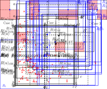
Figure 6: $R(u)$ (black) is the square centered at a blue point $u$. The Red shaded sub-squares of $R(u)$ contain some red points.

• Case 1: All other sub-squares of $R(u)$ contain red points. See Figure 5(b). Let $r_{1}\in R(u)_{NW}\cap{\cal P}_{r}$ and $r_{2}\in R(u)_{SE}\cap{\cal P}_{r}$ be two red points nearest to the line segments $\overline{us}$ and $\overline{ur}$, respectively. Let $R^{\prime}$ be a square whose left edge and bottom edge pass through the points $r_{1}$ and $r_{2}$, respectively. No feasible solution exists if $R^{\prime}_{NE}$ contains some red points. In this case, we set $R_{i}=\emptyset$ for $i\in[5]$. So, without loss of generality, assume that $R^{\prime}_{NE}$ contains no red points. Depending upon whether $R^{\prime}_{SW}$ contains some red points or not, we have the following two sub-cases.

  Case 1.1: $R^{\prime}_{SW}$ contains no red points (see Figure 5(b)). In this case, we set $R_{1}=R_{2}=R_{3}=R_{5}=\emptyset$ and $R_{4}=\text{U(SE)-R(NW)-MOVE}(\langle u,R^{\prime}\rangle)$ as defined in Algorithm 1.

  Case 1.2: $R^{\prime}_{SW}$ contains some red points (see figure 7(a)). In this case, we set $R_{4}=R_{5}=\emptyset$. Since $R(u)_{SW}\cap{\cal P}_{r}\neq\emptyset$ and $R(u)_{NE}\cap{\cal P}_{r}=\emptyset$, we defined the candidate squares $R_{1},R_{2}$ and $R_{3}$ as defined in Section 4.2.

• Case 2: $R(u)_{SW}$, and one of $R(u)_{NW}$ and $R(u)_{SE}$ contain red points. Assume, without loss of generality, $R(u)_{NW}$ contain some red points (see Figure 7(b)). For this case, we set $R_{4}=\emptyset$. Let $r^{\prime\prime}\in(R(u)_{NW}\cup R(u)_{SW})\cap{\cal P}_{r}$ be a red point nearest to the line segments $\overline{qs}$. If $r^{\prime\prime}\in R(u)_{SW}$, since $R(u)_{SW}\cap{\cal P}_{r}\neq\emptyset$ and $R(u)_{NE}\cap{\cal P}_{r}=\emptyset$, we define the candidate squares $R_{1},R_{2}$ and $R_{3}$ as defined in Section 4.2, and if $r^{\prime\prime}\in R(u)_{NW}$, since $R(u)_{NW}\cap{\cal P}_{r}\neq\emptyset$ and $R(u)_{SE}\cap{\cal P}_{r}=\emptyset$, we define the candidate squares $R_{1},R_{2}$ and $R_{3}$ in a similar way as defined in Section 4.2. Next, we define the candidate square $R_{5}$ irrespective of whether $r^{\prime\prime}\in R(u)_{SW}$ or $r^{\prime\prime}\in R(u)_{NW}$ (see Figure 8(a)). Let $H_{5}$ be a horizontal translated copy of $R(u)$ whose left edge passes through the point $r^{\prime\prime}$. Observe that $H_{5(NW)}\cup H_{5(SW)}$ contains no red point. Depending on which sub-squares among $H_{5(NE)}$ and $H_{5(SE)}$ contains some red points, we move $H_{5}$ as follows: (1) If $H_{5(NE)}$ and $H_{5(SE)}$ do not contain red points, we set $R_{5}=H_{5}$. (2) If $H_{5(NE)}$ and $H_{5(SE)}$ both sub-squares contain some red points, we set $R_{5}=\emptyset$. (3) Now, consider the case when exactly one of $H_{5(NE)}$ and $H_{5(SE)}$ contains some red points. W.l.o.g., assume that only $H_{5(SE)}$ contains some red points. The other case is similar. In this case, we set $R_{5}=\text{U(SE)-R(NW)-MOVE}(\langle u,H_{5}\rangle)$ as defined in Algorithm 1.

  

  (a)

  

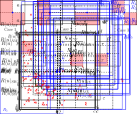
  (b)

  Figure 7: $R(u)$ (black) is the square centered at the blue point $u$. (a) Case 1.2: $R^{\prime}_{SW}$ contains some red points. Here, $R_{1}$, $R_{2}$ and $R_{3}$ are the candidate squares (blue) of $u$ constructed by using $R^{\prime}$ (black/dashed). (b) Case 2: $R(u)_{NW}$ and $R(u)_{SW}$ both contain some red points. Here, $R_{1}$, $R_{2}$ and $R_{3}$ are the candidate squares (blue) of $u$ constructed by using $R^{\prime}$ (black/dashed).

  

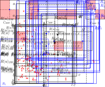
  (a)

  

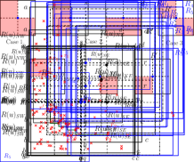
  (b)

  Figure 8: $R(u)$ (black) be the square centered at the blue point $u$. (a) Case 2: $R(u)_{NW}$ and $R(u)_{SW}$ both contain some red points. Here, $R_{5}$ is a candidate square (blue) of $u$. (b) Case 3: $R(u)_{NW}$ and $R(u)_{SE}$ both contain some red points. Here, $R_{4}$ and $R_{5}$ are the two candidate squares (blue) of $u$.

• Case 3: $R(u)_{NW}$ and $R(u)_{SE}$ both contain red points. See Figure 8(b). For this case, we set $R_{1}=R_{2}=R_{3}=\emptyset$. Let $r_{1}\in R(u)_{NW}\cap{\cal P}_{r}$ and $r_{2}\in R(u)_{SE}\cap{\cal P}_{r}$ be two red points nearest to the line segments $\overline{us}$ and $\overline{ur}$, respectively. Let $H_{4}$ be a square whose left and bottom edges pass through the points $r_{1}$ and $r_{2}$, respectively. Observe that $H_{4(SW)}$ contains no red points. If $H_{4(NE)}$ contains some red points, we set $R_{4}=\emptyset$. Otherwise, $H_{4(SE)}\cup H_{4(NW)}$ may contain some red points. Then, we set $R_{4}=\text{U(SE)-R(NW)-MOVE}(\langle u,H_{4}\rangle)$ as defined in Algorithm 1.

  Next, we define the candidate square $R_{5}$. Let $r_{3}\in R(u)_{NW}\cap{\cal P}_{r}$ and $r_{4}\in R(u)_{SE}\cap{\cal P}_{r}$ be two red points nearest to the line segments $\overline{up}$ and $\overline{uq}$, respectively (see Figure 8(b)). Let $H_{5}$ be a square whose top and right edges pass through the points $r_{3}$ and $r_{4}$, respectively. Observed that $H_{5(NE)}$ contains no red points. If $H_{5(SW)}$ contains some red points, we set $R_{5}=\emptyset$. Otherwise, $H_{5(SE)}\cup H_{5(NW)}$ may contain some red points. Then, we set $R_{5}=\text{D(NW)-L(SE)-MOVE}(\langle u,H_{5}\rangle)$, where D(NW)-L(SE)-MOVE is similar to U(SE)-R(NW)-MOVE, move the square downwards and leftwards instead of rightwards and upwards, respectively.

• Case 4: One of $R(u)_{NW}$, $R(u)_{SW}$ and $R(u)_{SE}$ contains red points. Assume, without loss of generality, $R(u)_{SW}$ contain some red points (see Figure 9(a)). Let $r^{\prime},r^{\prime\prime}\in R(u)_{SW}\cap{\cal P}_{r}$ be two red points nearest to the line segments $\overline{up}$ and $\overline{uq}$, respectively. If $r^{\prime}=r^{\prime\prime}$, we set the candidate squares $R_{1}$, $R_{2}$ and $R_{3}$ to be $\emptyset$. Otherwise, since $R(u)_{SW}\cap{\cal P}_{r}\neq\emptyset$ and $R(u)_{NE}\cap{\cal P}_{r}=\emptyset$, we obtain the candidate squares $R_{1},R_{2}$ and $R_{3}$ as defined in Section 4.2. Next, we define $R_{4}$ and $R_{5}$ irrespective of whether $r^{\prime}=r^{\prime\prime}$ or not (see Figure 9(b)). Let $H_{4}$ and $H_{5}$ be two vertical and horizontal translated copies of $R(u)$ such that the bottom edge of $H_{4}$ passes through $r^{\prime}$ and the left edge of $H_{5}$ passes through $r^{\prime\prime}$, respectively. Observe that $H_{5(NW)}\cup H_{5(SW)}$ contain no red point. Now, depending on which sub-squares among $H_{5(NE)}$ and $H_{5(SE)}$ contain red points, we move $H_{5}$ as follows: (1) If $H_{5(NE)}$ and $H_{5(SE)}$ both do not contain red points, we set $R_{5}=H_{5}$. (2) If $H_{5(NE)}$ and $H_{5(SE)}$ both sub-squares contain some red points, we set $R_{5}=\emptyset$. (3) Now, consider the case when exactly one of $H_{5(NE)}$ and $H_{5(SE)}$ contains some red points. W.l.o.g., assume that only $H_{5(SE)}$ contains some red points. The other case is similar. In this case, we set $R_{5}=\text{U(SE)-R(NW)-Move}(\langle u,H_{5}\rangle)$ as defined in Algorithm 1. Similarly, we define the candidate square $R_{4}$, which will be obtained by moving $H_{4}$.

  

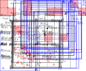
  (a)

  

  (b)

  Figure 9: $R(u)$ (black) be the square centered at the blue point $u$. Case 4: $R(u)_{SW}$ contains some red points. (a) $R_{1}$, $R_{2}$ and $R_{3}$ are the candidate squares (blue) of $u$ constructed by using $R^{\prime}=R(u)$. (b) $R_{4}$ and $R_{5}$ are the two candidate squares (blue) of $u$.

From the above description, we have that for any blue point $u$, we have $0\leq|{\mathcal{S}}(u)|\leq 5$, and each (non-empty) candidate square of $u$ always contains $u$ but no red points. Later, we will show that if a blue point $u$ can be covered by a square in the optimum, at least one candidate square exists, i.e. ${\mathcal{S}}(u)\neq\emptyset$.

4.4 Algorithm Description

The algorithm always maintains a set ${\mathcal{S}}_{i}$ of ${\cal P}_{r}$-empty squares to cover all the blue points $\{u_{1},u_{2},\ldots,u_{i}\}$ that have been part of the input so far. Note that, initially, ${\mathcal{S}}_{0}=\emptyset$. The description of the algorithm is given in Algorithm 3.

Algorithm 3 An online algorithm for the class cover problem

1:${\mathcal{S}}_{0}\leftarrow\emptyset$

2:for $i=1$ to $\infty$ do $\triangleright$ arrival of a blue point $u_{i}$

3:     if $u_{i}$ is not covered by ${\mathcal{S}}_{i-1}$ then

4:         ${\mathcal{S}}_{i}\leftarrow{\mathcal{S}}_{i-1}\cup{\mathcal{S}}(u_{i})$ $\triangleright$ ${\mathcal{S}}(u_{i})$ is the set of candidate squares of $u_{i}$

5:     else

6:         ${\mathcal{S}}_{i}\leftarrow{\mathcal{S}}_{i-1}$

7:     end if

8:end for

5 Analysis of the Online Algorithm

In this section, we analyse the performance of Algorithm 3. First, in Section 5.1, we give the correctness of the algorithm. There, we mention important structural properties of candidate squares in Lemma 1. Then, in Section 5.2, using this lemma, we give a simpler analysis to show that the competitive ratio of the algorithm is $\max\{6,20\log_{2}(m)\}$. Finally, in Section 5.3, we give a tighter analysis to reach the competitive ratio to $\max\{6,10+10\log_{2}(m)\}$.

5.1 Correctness of the Algorithm

Let OPT$({\cal I})$ be an optimal solution of the class cover problem given by an offline algorithm for an input sequence ${\cal I}$ of blue points. Let ${\cal O}=\square o_{1}o_{2}o_{3}o_{4}$ be a square in OPT$({\cal I})$ centered at $o$. Let $o_{5},o_{6},o_{7}$ and $o_{8}$ are the midpoints of the edges $o_{1}o_{2},o_{2}o_{3},o_{3}o_{4}$ and $o_{4}o_{1}$ of ${\cal O}$, respectively.

Let $u$ be an input blue point lying inside ${\cal O}$. Without loss of generality, we assume that $u\in{\cal O}_{SW}$. Then in the next lemma, we will prove that ${\mathcal{S}}(u)\neq\emptyset$, which guarantees that the Algorithm 3 indeed outputs a valid solution. In this lemma, we also mention important structural properties of the candidate squares of $u$, which are essential to obtain the required competitive ratio in the subsequent subsection.

Lemma 1.

Let $u$ be an input blue point in ${\cal O}_{SW}$. Then, at least one non-empty candidate square of $u$ exists, i.e. ${\mathcal{S}}(u)\neq\emptyset$. In addition, one of the following properties holds.

1. At least one Type 2 candidate square of $u$ contains ${\cal O}_{SW}$.

   or,

2. 1. ${\cal Q}(u)_{SW}\cap R(u)_{SW}\neq\emptyset$ and $\mathcal{PS}(u)_{SW}\neq\emptyset$.

   2. There exists a square $P\in\mathcal{PS}(u)_{SW}$ that contains ${\cal O}_{SW}$.

   3. There exist three Type 1 candidate squares $R_{1},R_{2}$ and $R_{3}$ of $u$ (they may not be distinct), obtained by moving three squares $H_{1},H_{2}$ and $H_{3}\in\mathcal{PS}(u)_{SW}$, respectively, such that $R_{i}\neq\emptyset$ for all $i$.

   4. If $H_{i}$, at first, contains ${\cal O}_{SW}$, then $R_{i}$ contains ${\cal O}_{SW}$. Moreover, either the left edge of $R_{i}$ is to the right side of the left edge of $H_{i}$ or the bottom edge of $R_{i}$ is above the bottom edge of $H_{i}$.

   5. If $H_{i}$, at first, contains ${\cal O}_{NW}$, then $R_{i}$ contains either ${\cal O}_{NW}$ or ${\cal O}_{SW}$, and the bottom edge of $R_{i}$ does not lie above the bottom edge of $H_{i}$.

   6. Similarly, if $H_{i}$, at first, contains ${\cal O}_{SE}$, then $R_{i}$ contains either ${\cal O}_{SE}$ or ${\cal O}_{SW}$, and the left edge of $R_{i}$ does not lie on the right side of the left edge of $H_{i}$.

   7. Either at least one $R_{i}$ contains ${\cal O}_{SW}$ or $\bigcup_{i=1}^{3}R_{i}$ contains ${\cal O}_{NW}\cup{\cal O}_{SE}$.

Proof.

First note that, as $R(u)$ and ${\cal O}$ are translated copies of each other, and $u\in{\cal O}_{SW}$, we have that $R(u)$ contains ${\cal O}_{SW}$. Now, if $R(u)\cap{\cal P}_{r}=\emptyset$, then according to Section 4.3, we have ${\mathcal{S}}(u)=\{R(u)\}$, and $R(u)$ contains ${\cal O}_{SW}$. In this case, property P1 holds. So, w.l.o.g., assume that at least one sub-squares of $R(u)$ contains some red points. But observe that as $R(u)_{NE}$ is contained in ${\cal O}$, the sub-square $R(u)_{NE}$ contains no red points. Now, we have the following sub-cases depending on which sub-squares of $R(u)$, except $R(u)_{NE}$, contain red points (see Figure 10).

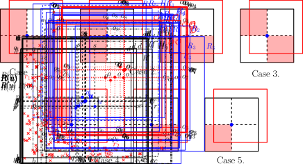
Figure 10: ${\cal O}$ (red) is an optimum square and $R(u)$ (black) be the square centered at a blue point $u$. The Red shaded sub-squares of $R(u)$ contain some red points.

• Case 1: Only $R(u)_{NE}$ contains no red points. Let $r_{1}\in R(u)_{NW}\cap{\cal P}_{r}$ and $r_{2}\in R(u)_{SE}\cap{\cal P}_{r}$ be two red points nearest to the line segments $\overline{us}$ and $\overline{ur}$, respectively (see Figure 11(a)). As defined in Section 4.3 (Case 1), consider the square $R^{\prime}$ whose left edge and bottom edge pass through the points $r_{1}$ and $r_{2}$, respectively.

  Claim 1.

  ${\cal O}\cap R(u)\subseteq R^{\prime}$, and $R^{\prime}$ contains ${\cal O}_{SW}$.

  Proof.

  Observe that the left edge of $R^{\prime}$ lies between the left edge of $R(u)$ and the left edge of ${\cal O}$. Similarly, the bottom edge of $R^{\prime}$ lies between the bottom edge of $R(u)$ and the bottom edge of ${\cal O}$. Due to this, $R^{\prime}$, a translated copy of both $R(u)$ and ${\cal O}$, contains $R(u)\cap{\cal O}$. Now, since $R(u)$ contains ${\cal O}_{SW}$ and ${\cal O}\cap R(u)\subseteq R^{\prime}$, we have that $R^{\prime}$ contains ${\cal O}_{SW}$. ∎

  Due to the above claim, $R^{\prime}_{NE}$ contains no red point. Now, depending on whether $R^{\prime}_{SW}$ contains some red points or not, we have the following two sub-cases.

  

  (a)

  (b)

  Figure 11: ${\cal O}$ (red) be an optimum square and $R(u)$ (black) be the square centered at the blue point $u$. (a) Case 1.1: $R^{\prime}_{SW}(u)$ contains no red points. Then, $R_{4}$ (blue) is a candidate square of $u$ that contains ${\cal O}_{SW}$. (b) Case 1.2: The square $P$ (blue) contains ${\cal O}_{SW}$.

  Case 1.1: $R^{\prime}_{SW}$ contains no red point (see Figure 11(a)). So, only $R^{\prime}_{NW}\cup R^{\prime}_{SE}$ may contain some red points. In that case (see Section 4.3 (Case 1.1)), we call U(SE)-R(NW)-MOVE$(\langle u,R^{\prime}\rangle)$. Since the left edge of $R^{\prime}$ lies to the left side of the left edge of ${\cal O}$ and the square ${\cal O}$ is red points free, we have that $R^{\prime}$ will be moved rightwards until $R^{\prime}_{NW}$ becomes red points free or the left edge of $R^{\prime}$ touches the left edge of ${\cal O}$. Similarly, since the bottom edge of $R^{\prime}$ lies below the bottom edge of ${\cal O}$ and the square ${\cal O}$ is red points free, we have that $R^{\prime}$ will be moved upwards until $R^{\prime}_{SE}$ becomes red points free or the bottom edge of $R^{\prime}$ touches the bottom edge of ${\cal O}$. Also, observe that during the movement of $R^{\prime}$, the sub-squares $R^{\prime}_{NE}$ and $R^{\prime}_{SW}$ never contain a red point. Therefore, during the movement of $R^{\prime}$, we are guaranteed to find a candidate square that contains $u$ but no red points, and we set such a square as a candidate square $R_{4}$ of $u$. Hence, ${\mathcal{S}}(u)\neq\emptyset$. Note that during the movement of $R^{\prime}$, the left edge of $R^{\prime}$ lies always to the left side of the left edge of ${\cal O}$, and the bottom edge of $R^{\prime}$ lies always below the bottom edge of ${\cal O}$. Therefore, $R^{\prime}$ always contains ${\cal O}_{SW}$, and thus, $R_{4}$ also contains ${\cal O}_{SW}$. So, in this case, property P1 holds.

  Case 1.2: $R^{\prime}_{SW}$ contains some red points (see Figure 11(b)). In this case, we define the Type 1 candidate squares of $u$ (see Section 4.3 (Case 1.2)). For this (as defined in Section 4.1), consider the set of $SW$ staircase points ${\cal Q}(u)_{SW}$ and the set of $SW$ possible candidate squares $\mathcal{PS}(u)_{SW}$ of $u$. Observe that the red points in $R^{\prime}_{SW}$ must belong to $R(u)_{SW}$ because of the definitions of $r_{1},r_{2}$ and $R^{\prime}$. Therefore, $R(u)_{SW}\cap R^{\prime}_{SW}\cap{\cal P}_{r}\neq\emptyset$. As a result, ${\cal Q}(u)_{SW}\cap R(u)_{SW}\neq\emptyset$. Let ${\cal Q}(u)_{SW}=\{r_{1},q_{0},q_{1},\dots,q_{k},r_{2}\}$ be the set of $SW$ staircase points of $u$ such that for each $i\in\{0\}\cup[k]$, the point $q_{i}\in R(u)_{SW}\cap R^{\prime}_{SW}\cap{\cal P}_{r}$.

  Since $r_{1}$ lies on the left side of the left edge of ${\cal O}$ and the point $r_{2}$ lies below the bottom edge of ${\cal O}$ and all the points $q_{0},q_{1},\dots,q_{k}\in R(u)_{SW}\cap R^{\prime}_{SW}\cap{\cal P}_{r}$, we have two consecutive red points, say $x_{1}$ and $x_{2}$, among $\{q_{0},q_{1},\dots,q_{k}\}$ such that $x_{1}$ lies on the left side of the left edge of ${\cal O}$, and $x_{2}$ lies below the bottom edge of ${\cal O}$ (see Figure 11(b)). So, consider the square $P$ whose left edge contains $x_{1}$ and the bottom edge contains $x_{2}$. In a similar way as in Claim 1, we can prove that $R(u)\cap{\cal O}\subseteq P$, and $P$ contains ${\cal O}_{SW}$. As a result, $P_{NE}$ lies inside ${\cal O}$, so it does not contain any red points. Therefore, there exists at least one possible candidate square of $u$, i.e. $P\in\mathcal{PS}(u)_{SW}$ and $\mathcal{PS}(u)_{SW}\neq\emptyset$. Hence, P2(a) and P2(b) hold.

  Assume $\mathcal{PS}(u)_{SW}=\{P_{1},\dots,P_{k^{\prime}}\}$, for some integer $k^{\prime}$, be the set of $SW$ possible candidate squares of $u$. Now, consider the three possible candidate squares $H_{1}=P_{1},H_{2}=P_{\lceil\frac{k^{\prime}}{2}\rceil}$ and $H_{3}=P_{k^{\prime}}$ (as defined in Section 4.2). Let us assume that $P=P_{i}$ for some $i\in[k^{\prime}]$.

  

  (a)

  

  (b)

  Figure 12: ${\cal O}$ (red) be an optimum square and $R(u)$ (black) be the square centered at the blue point $u$. (a) Case 1.2: The square $H_{1}$ (blue/dashed) is a possible candidate square of $u$ that contains ${\cal O}_{NW}$, and $R_{1}$ (blue) is a candidate square of $u$, obtained from $H_{1}$, also contains ${\cal O}_{NW}$. (b) Case 1.2: $R^{\prime}_{SW}$ contains some red points. Then, $R_{1},R_{2}$ and $R_{3}$ (blue) are the candidate squares of $u$ that contains ${\cal O}_{NW}\cup{\cal O}_{SE}$, constructed by using $R^{\prime}$ (black/dashed).

  Now, we claim that $H_{1}$ contains either ${\cal O}_{NW}$ or ${\cal O}_{SW}$ (see Figure 12(a)). Since the $SW$ vertex of $H_{1}$ lies in $R(u)_{SW}$, the left edge of $H_{1}$ lies to the right side of the left edge of $R(u)$. Again since $P=P_{i}$ contains ${\cal O}_{SW}$, thus the left edge of $H_{1}=P_{1}$ lies to the left side of the left edge of ${\cal O}$. Therefore, the right edge of $H_{1}$ lies between the right edge of $R(u)$ and the right edge of ${\cal O}$. Similarly, the bottom edge of $H_{1}$ lies between the line segment $\overline{pr}$ and the bottom edge of $P$. Since $u\in{\cal O}_{SW}$ and $P$ contains ${\cal O}_{SW}$, the bottom edge of ${\cal O}$ also lies between the line segment $\overline{pr}$ and the bottom edge of $P$. Now, if the bottom edge of $H_{1}$ lies above the bottom edge of ${\cal O}$, then $H_{1}$ contains ${\cal O}_{NW}$; otherwise, $H_{1}$ contains ${\cal O}_{SW}$. Using similar argument, we can show that if $i\geq\lceil\frac{k^{\prime}}{2}\rceil$, the square $H_{2}$ contains either ${\cal O}_{NW}$ or ${\cal O}_{SW}$, and if $i\leq\lceil\frac{k^{\prime}}{2}\rceil$, the square $H_{2}$ contains either ${\cal O}_{SW}$ or ${\cal O}_{SE}$. Also, the square $H_{3}$ contains either ${\cal O}_{SW}$ or ${\cal O}_{SE}$.

  Now, suppose that $H_{j}$ contains ${\cal O}_{NW}$ (see Figure 12(a)). Here, we argue the existence of $R_{j}$. If $H_{j}$ contains no red points, then $R_{j}=H_{j}\in{\mathcal{S}}(u)$. Otherwise, $H_{j}$ contains some red points. Due to Observation 2 and the fact that $H_{j}$ contains ${\cal O}_{NW}$, we have that only $H_{j(NW)}$ contains some red points. In that case, we call ST-R(NW)-MOVE$(\langle u,H_{j}\rangle)$. Here, we move it rightwards along the staircase $ST_{SW}({\cal Q}(u)_{SW})$ until $H_{j(NW)}\cup H_{j(NE)}$ becomes red points free. After that, if $H_{j(SE)}$ contains some red point, then we call U(SE)-R(NW)-MOVE$(\langle u,H_{j}\rangle)$. Hence, before the left edge of $H_{j}$ touches the left edge of ${\cal O}$, either $H_{j}$ becomes red points free or $H_{j(SE)}$ contains some red points. In the former case, we set $R_{j}=H_{j}$, and in the latter case, the existence of the candidate square $R_{j}$ of $u$ can be shown in a similar way as Case 1.1. Similarly, we can show the existence of a candidate square of $u$ when $H_{j}$ contains ${\cal O}_{SW}$ or ${\cal O}_{SE}$. Therefore, P2(c) holds.

  Assuming $H_{j}$, at first, contains ${\cal O}_{NW}$, here we argue that $R_{j}$ contains either ${\cal O}_{NW}$ or ${\cal O}_{SW}$ (see Figure 12(a)). Recall that in this case, during the movement of $H_{j}$, the left edge of $H_{j}$ always lies between the left edge of ${\cal O}$ and the left edge of $R(u)$. Therefore, the left edge of $H_{j}$ never lies on the right side of the left edge of ${\cal O}$. As a result, $H_{j}$, a translated copy of ${\cal O}$, always contains either ${\cal O}_{NW}$ or ${\cal O}_{SW}$. Thus, $R_{j}$ contains either ${\cal O}_{NW}$ or ${\cal O}_{SW}$.

  

  (a)

  

  (b)

  Figure 13: ${\cal O}$ (red) be an optimum square and $R(u)$ (black) be the square centered at the blue point $u$. (a) Case 2.1: $R(u)_{NW}$ and $R(u)_{SW}$ contain some red points such that $r^{\prime\prime}$ does not lie on the left side of the left edge of ${\cal O}$. Then, $R_{1}$, $R_{2}$ and $R_{3}$ (blue) are the candidate squares of $u$ that contains ${\cal O}_{NW}\cup{\cal O}_{SE}$, constructed by using $R^{\prime}$ (black/dashed). (b) Case 2.2: $R(u)_{NW}$ and $R(u)_{SW}$ contain some red points such that $r^{\prime\prime}$ lies on the left side of the left edge of ${\cal O}$. Then, $R_{5}$ (blue) is a candidate square of $u$ that contains ${\cal O}_{SW}$, obtained by moving the square $H_{5}$ (black/dashed).

  Assuming $H_{j}$, at first, contains ${\cal O}_{NW}$, here we argue that the bottom edge of $R_{j}$ does not lie above the bottom edge of $H_{j}$ (see Figure 12(a)). In this case, the square $H_{j}$, at first, is moved in the rightward direction along the staircase, and when it is moved in the upwards direction, the bottom edge of $H_{j}$ already lies below the bottom edge of ${\cal O}$. So, it is moved upwards until the bottom edge of $H_{j}$ touches the bottom edge of ${\cal O}$. Since, at first, the bottom edge of $H_{j}$ lies above the bottom edge of ${\cal O}$, the bottom edge of $R_{j}$ does not lie above the bottom edge of $H_{j}$. Therefore, P2(e) holds. Similarly, we can prove that P2(d) and P2(f) also hold.

  Since $H_{1}$, at first, contains either ${\cal O}_{NW}$ or ${\cal O}_{SW}$, then $R_{1}$ contains either ${\cal O}_{NW}$ or ${\cal O}_{SW}$. Since $H_{3}$, at first, contains either ${\cal O}_{SW}$ or ${\cal O}_{SE}$, then $R_{3}$ contains either ${\cal O}_{SW}$ or ${\cal O}_{SE}$. Therefore, we have either at least one $R_{j}$ contains ${\cal O}_{SW}$ or $\bigcup_{j=1}^{3}R_{j}$ contains ${\cal O}_{NW}\cup{\cal O}_{SE}$ (see Figure 12(b)), and so P2(g) holds. So, in this case, we have shown that property P2 holds.

• Case 2: $R(u)_{SW}$ contains some red points, and one of $R(u)_{NW}$ and $R(u)_{SE}$ contains no red point. W.l.o.g., assume that $R(u)_{SE}$ contains no red points; the other case is similar. Let $r^{\prime\prime}\in(R(u)_{NW}\cup R(u)_{SW})\cap{\cal P}_{r}$ be a red point nearest to the line segments $\overline{qs}$ (see Figure 13(a)). Now, depending on the position of $r^{\prime\prime}$, we have the following two sub-cases.

  Case 2.1: The red point $r^{\prime\prime}$ lies on the right side of the left edge of ${\cal O}$. Hence, $r^{\prime\prime}\in R(u)_{SW}\cap{\cal P}_{r}$. In this case, we define the Type 1 candidate squares of $u$ (see Section 4.3 (Case 2)). For this (as defined in Section 4.1), consider the set of $SW$ staircase points ${\cal Q}(u)_{SW}$ and the set of $SW$ possible candidate squares $\mathcal{PS}(u)_{SW}$ of $u$. Now, as defined in Section 4.1, consider the square $R^{\prime}$ whose left edge and bottom edge pass through the points $r_{1}$ and $c$ (recall that $R(u)_{SE}$ contains no red points), respectively, where $r_{1}\in R(u)_{NW}\cap{\cal P}_{r}$ be a red point nearest to the line segments $\overline{us}$. Observe that $R^{\prime}$ is a horizontal translated copy of $R(u)$ whose left edge passes through the point $r_{1}$.

  Claim 2.

  ${\cal O}\cap R(u)\subseteq R^{\prime}$, and $R^{\prime}$ contains ${\cal O}_{SW}$.

  Proof.

  Observe that the left edge of $R^{\prime}$ lies between the left edge of $R(u)$ and the left edge of ${\cal O}$. As a result, we have that $R^{\prime}$, a horizontal translated copy of both $R(u)$ and ${\cal O}$, contains $R(u)\cap{\cal O}$. Since $R(u)$ contains ${\cal O}_{SW}$ and ${\cal O}\cap R(u)\subseteq R^{\prime}$, we have that $R^{\prime}$ contains ${\cal O}_{SW}$. ∎

  Due to Claim 2, $R^{\prime}_{NE}$ does not contain any red points. But $r^{\prime\prime}\in R^{\prime}_{SW}$ i.e. $R^{\prime}_{SW}$ contains some red points. Therefore, $R(u)_{SW}\cap R^{\prime}_{SW}\cap{\cal P}_{r}\neq\emptyset$. As a result, ${\cal Q}(u)_{SW}\cap R(u)_{SW}\neq\emptyset$. Now, in a similar way as to above Case 1.2, we can show that the candidate squares $R_{1}$, $R_{2}$ and $R_{3}$ exist, and property P2 also holds.

  Case 2.2: The red point $r^{\prime\prime}$ lies on the left side of the left edge of ${\cal O}$, then as defined in Section 4.3 (Case 2), we consider a square $H_{5}$, a horizontal translated copy of $R(u)$, whose left edge passes through the point $r^{\prime\prime}$ (see Figure 13(b)). In a similar way as in Claim 2, we can show that ${\cal O}\cap R(u)\subseteq H_{5}$, and $H_{5}$ contains ${\cal O}_{SW}$. Due to this, $H_{5(NE)}$ contains no red point. Observe that only $H_{5(SE)}$ may contain some red points. In that case, we call U(SE)-R(NW)-MOVE$(\langle u,H_{5}\rangle)$. Therefore, the existence of the candidate square $R_{5}$ of $u$ and the fact that $R_{5}$ contains ${\cal O}_{SW}$ can be shown similarly to the above Case 1.1. Hence, ${\mathcal{S}}(u)\neq\emptyset$, and property P1 holds.

  

  (a)

  

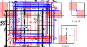
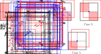
  (b)

  Figure 14: ${\cal O}$ (red) be an optimum square and $R(u)$ (black) be the square centered at the blue point $u$. (a) Case 3: $R_{NW}(u)$ and $R_{SE}(u)$ both contain some red points. Then, $R_{4}$ (blue) is a candidate square of $u$ that contains ${\cal O}_{SW}$, obtained by moving the square $H_{4}$ (blue/dashed). (b) Case 4: Only $R_{NW}(u)$ contains some red points. Then, $R_{5}$ (blue) is a candidate square of $u$ that contains ${\cal O}_{SW}$, obtained by moving the square $H_{5}$ (black/dashed).

• Case 3: $R(u)_{SW}$ contains no red points, but both $R(u)_{NW}$ and $R(u)_{SE}$ contain some red points. Let $r_{1}\in R(u)_{NW}\cap{\cal P}_{r}$ and $r_{2}\in R(u)_{SE}\cap{\cal P}_{r}$ be two red points nearest to the line segments $\overline{us}$ and $\overline{ur}$, respectively (see Figure 14(a)). Then as defined in Section 4.3 (Case 3), we consider the square $H_{4}$ whose left and bottom edge pass through the points $r_{1}$ and $r_{2}$, respectively. In a similar way as in Claim 1, we can show that ${\cal O}\cap R(u)\subseteq H_{4}$, and $H_{4}$ contains ${\cal O}_{SW}$. Due to this, $H_{4(NE)}$ contains no red point. Note that $H_{4(NW)}\cup H_{4(SE)}$ may contains some red points. If $H_{4(NW)}\cup H_{4(SE)}$ contains some red points, we call U(SE)-R(NW)-MOVE$(\langle u,H_{4}\rangle)$. Therefore, the existence of the candidate square $R_{4}$ of $u$ and the fact that $R_{4}$ contains ${\cal O}_{SW}$ can be shown similarly to the above Case 1.1. Hence, ${\mathcal{S}}(u)\neq\emptyset$, and property P1 holds.

• Case 4: $R(u)_{SW}$ contains no red points, and one of $R(u)_{NW}$ and $R(u)_{SE}$ contains some red points. W.l.o.g., assume that $R(u)_{NW}$ contains some red points; the other case is similar. Let $r^{\prime}\in R(u)_{NW}\cap{\cal P}_{r}$ be a red point nearest to the line segments $\overline{us}$ (see Figure 14(b)). Then as defined in Section 4.3 (Case 4), we consider the square $H_{5}$, a horizontal translated copy of $R(u)$, whose left edge passes through $r^{\prime}$. In a similar way as in Claim 2, we can show that ${\cal O}\cap R(u)\subseteq H_{5}$, and $H_{5}$ contains ${\cal O}_{SW}$. Due to this, $H_{5(NE)}$ contains no red point. Note that only $H_{5(SE)}$ may contain some red points. If $H_{5(SE)}$ contains some red points, we call U(SE)-R(NW)-MOVE$(\langle u,H_{5}\rangle)$. Therefore, the existence of the candidate square $R_{5}$ of $u$ and the fact that $R_{5}$ contains ${\cal O}_{SW}$ can be shown similarly to the above Case 1.1. Hence, ${\mathcal{S}}(u)\neq\emptyset$, and property P1 holds.

  

  (a)

  

  (b)

  Figure 15: ${\cal O}$ (red) be an optimum square and $R(u)$ (black) be the square centered at the blue point $u$. (a) Case 5.1: Only $R_{SW}(u)$ contains some red points, and both $r^{\prime},r^{\prime\prime}$ lie on the left side of $a_{1}a_{2}$. Then, $R_{5}$ (blue) is a candidate square of $u$ that contains ${\cal O}_{SW}$, obtained by moving the square $H_{5}$ (black/dashed). (b) Case 5.3: Only $R_{SW}(u)$ contains some red points, and the points $r^{\prime}$ and $r^{\prime\prime}$ are distinct such that exactly one of $r^{\prime}$ and $r^{\prime\prime}$ lies to the left side of the left edge of ${\cal O}$ and other one lies below the bottom edge of ${\cal O}$. Then, $R_{1},R_{2}$ and $R_{3}$ (blue) are the candidate squares of $u$ that contains ${\cal O}_{NW}\cup{\cal O}_{SE}$, constructed by using $R^{\prime}$.

• Case 5: $R(u)_{SW}$ contains some red points, but $R(u)_{SE}\cup R(u)_{NW}$ contains no red points. Let $r^{\prime},r^{\prime\prime}\in R(u)_{SW}\cap{\cal P}_{r}$ be two red points nearest to the line segments $\overline{up}$ and $\overline{uq}$, respectively (see Figure 15(a)). Now depending on the position of $r^{\prime}$ and $r^{\prime\prime}$, we have the following three sub-cases.

  Case 5.1: The red points $r^{\prime}$ and $r^{\prime\prime}$ both lie on the left side of the left edge of ${\cal O}$ (see Figure 15(a)). We consider the square $H_{5}$, a horizontal translated copy of $R(u)$, whose left edge passes through the point $r^{\prime\prime}$ (see Section 4.3 (Case 4)). In a similar way as in Claim 2, we can show that ${\cal O}\cap R(u)\subseteq H_{5}$, and $H_{5}$ contains ${\cal O}_{SW}$. Due to this, $H_{5(NE)}$ contains no red point. Note that only $H_{5(SE)}$ may contain some red points. In that case, we call U(SE)-R(NW)-MOVE$(\langle u,H_{5}\rangle)$. Now, the existence of the candidate square $R_{5}$ of $u$ and the fact that $R_{5}$ contains ${\cal O}_{SW}$ can be shown similarly to the above Case 1.1. Hence, ${\mathcal{S}}(u)\neq\emptyset$, and property P1 holds.

  Case 5.2: The red points $r^{\prime}$ and $r^{\prime\prime}$ both lie below the bottom edge ${\cal O}$. In this case, in a similar way as in the above Case 5.1, we can prove the existence of the candidate square $R_{4}$, and the fact that $R_{4}$ contains ${\cal O}_{SW}$. Hence, property P1 also holds.

  Case 5.3: The red points $r^{\prime}$ and $r^{\prime\prime}$ are distinct such that exactly one of $r^{\prime}$ and $r^{\prime\prime}$ lies to the left side of the left edge of ${\cal O}$ and other one lies below the bottom edge of ${\cal O}$ (see Figure 15(b)). In this case, we define the Type 1 candidate squares of $u$ (see Section 4.3 (Case 4)). For this (as defined in Section 4.1), consider the set of $SW$ staircase points ${\cal Q}(u)_{SW}$ and the set of $SW$ possible candidate squares $\mathcal{PS}(u)_{SW}$ of $u$. Now, as defined in Section 4.1, consider the square $R^{\prime}$ whose left edge and bottom edge pass through the points $a$ and $c$, respectively (recall that both sub-squares $R(u)_{NW}$ and $R(u)_{SE}$ contain no red points). Observe that $R^{\prime}=R(u)$. Therefore, $R^{\prime}_{SW}$ contains some red points. As a result, ${\cal Q}(u)_{SW}\cap R(u)_{SW}\neq\emptyset$. Now, in a similar way as to above Case 1.2, we can show that the candidate squares $R_{1}$, $R_{2}$ and $R_{3}$ exist, and property P2 also holds.

So the lemma follows. ∎

5.2 Competitive Analysis

In the following lemma, we prove that to cover all the blue points contained in ${\cal O}_{SW}$, the Algorithm 3 needs at most $5\log_{2}(m)$ squares, where $m\geq 2$.

Lemma 2.

The Algorithm 3 needs at most $5\log_{2}(m)$ candidate squares to cover all the blue points in ${\cal O}_{SW}$, where $m\ (\geq 2)$ is the number of red points.

(a)

(b)

Figure 16: ${\cal O}$ (red) is an optimum square and $R(u)$ (black) be the square centered at the blue point $u$. (a) Both the squares $H_{1}$ (blue/dashed) and $R^{(1)}_{1}$ (blue) contain ${\cal O}_{NW}$ (green shaded area). Also, the possible candidate square $P^{(1)}_{i}$ (dark green) contain ${\cal O}_{SW}$ (yellow shaded area). (b) The candidate square $R^{(1)}_{1}$ (blue) of $u_{1}$ contains $(R(u_{1})_{NW}\cup R(u_{1})_{NE})\cap{\cal O}_{SW}$ (green shaded area).

Proof.

Let $u_{1},u_{2},\dots,u_{k}$ be the largest sub-sequence of the input sequence such that for each $i\in[k]$, $u_{i}\in{\cal O}_{SW}$ and it is uncovered upon its arrival. If any candidate square of $u_{1}$ contains ${\cal O}_{SW}$, then the lemma follows. W.l.o.g., assume that none of the candidate squares of $u_{1}$ contains ${\cal O}_{SW}$. Thus, due to Lemma 1 (P2(a)), we have $\mathcal{PS}(u_{1})_{SW}\neq\emptyset$. Let $\mathcal{PS}(u_{1})_{SW}=\{P^{(1)}_{1},$ $P^{(1)}_{2},\dots,P^{(1)}_{k_{1}}\}$, for some integer $k_{1}\leq m$, be the set of possible candidate squares of $u_{1}$ constructed by using the staircase points set ${\cal Q}(u_{1})_{SW}$. Let $R_{1}^{(1)},R_{2}^{(1)},$ $R_{3}^{(1)}~{}\in~{}{\mathcal{S}}(u_{1})$ be the three candidate squares obtained by moving three possible candidate squares $H_{1},H_{2}$ and $H_{3}$, respectively, where $H_{1}=P^{(1)}_{1},H_{2}=P^{(1)}_{\lceil\frac{k_{1}}{2}\rceil}$ and $H_{3}=P^{(1)}_{k_{1}}$. Note that due to Lemma 1 (P2(g)), $\bigcup_{j=1}^{3}R_{j}^{(1)}$ contains ${\cal O}_{NW}\cup{\cal O}_{SE}$. As a result, $u_{1}$ has at least two distinct candidate squares. From Lemma 1 (P2(b)), we have a possible candidate square of $u_{1}$, say $P^{(1)}_{i}\in\mathcal{PS}(u_{1})_{SW}$, for some $i\in[k_{1}]$, that contains ${\cal O}_{SW}$ (see Figure 16(a)). Now, we claim that $H_{1}$ contains ${\cal O}_{NW}$, and the square $H_{3}$ contains ${\cal O}_{SE}$.

Claim 3.

1. The possible candidate square $H_{1}=P^{(1)}_{1}$ contains ${\cal O}_{NW}$.

2. The possible candidate square $H_{3}=P^{(1)}_{k_{1}}$ contains ${\cal O}_{SE}$.

Proof.

(i) Since the $SW$ vertex of $H_{1}$ lies in $R(u_{1})_{SW}$, the left edge of $H_{1}$ lies on the right side of the left edge of $R(u_{1})$ (see Figure 16(a)). Again, since $P^{(1)}_{i}$ contains ${\cal O}_{SW}$, the left edge of $H_{1}=P^{(1)}_{1}$ lies on the left side of the left edge of ${\cal O}$. Therefore, the right edge of $H_{1}$ lies between the right edge of $R(u_{1})$ and the right edge of ${\cal O}$. Similarly, the bottom edge of $H_{1}$ lies between the top edge of $R(u_{1})_{SW}$ and the bottom edge of $P^{(1)}_{i}$. Since the blue point $u_{1}\in{\cal O}_{SW}$ and $P^{(1)}_{i}$ contains ${\cal O}_{SW}$, we have that the bottom edges of ${\cal O}$ also lies between the top edge of $R(u_{1})_{SW}$ and the bottom edge of $P^{(1)}_{i}$. Since $R_{1}^{(1)}$ does not contain ${\cal O}_{SW}$, from Lemma 1 (P2(d)), we have that $H_{1}$ also does not contain ${\cal O}_{SW}$. As a result, the bottom edge of $H_{1}$ lies above the bottom edge of ${\cal O}$; therefore, $H_{1}$, a translated copy of ${\cal O}$, contains ${\cal O}_{NW}$.

(ii) We can prove this in a similar way as (i). ∎

Due to Claim 3 and Lemma 1 (P2(e)), the candidate square $R_{1}^{(1)}$ contains either ${\cal O}_{NW}$ or ${\cal O}_{SW}$. Recall that none of the candidate squares of $u_{1}$ contains ${\cal O}_{SW}$. Thus, the candidate square $R_{1}^{(1)}$ contains ${\cal O}_{NW}$ (see Figure 16(a)). Similarly due to Lemma 1 (P2(f)) and Claim 3, the candidate square $R_{3}^{(1)}$ contains ${\cal O}_{SE}$.

(a)

(b)

Figure 17: ${\cal O}$ (red) is an optimum square and $R(u)$ (black) be the square centered at the blue point $u$. (a) The blue point $u_{2}$ does not lie in the possible candidate square $P^{(1)}_{2}$ (dark green) of $u_{1}$. (b) $R^{\prime(1)}$ (black/dashed) is a square whose left edge and the bottom edge pass through the points $q_{1}^{(1)}$ and $q_{2}^{(1)}$, respectively, and ${\cal Q}(u_{1})_{SW}$ is the set of all the red (cross) points lying in the staircase (dark green/dashed).

Since $R_{2}^{(1)}$ does not contain ${\cal O}_{SW}$, the possible candidate square $H_{2}=P^{(1)}_{\lceil\frac{k_{1}}{2}\rceil}$ also does not contain ${\cal O}_{SW}$ (due to Lemma 1 (P2(d))). Recall that, the possible candidate square $P^{(1)}_{i}\in\mathcal{PS}(u_{1})_{SW}$ contains ${\cal O}_{SW}$. As a result, $i\neq\lceil\frac{k_{1}}{2}\rceil$.

Claim 4.

1. If $i>\lceil\frac{k_{1}}{2}\rceil$, the possible candidate square $H_{2}=P^{(1)}_{\lceil\frac{k_{1}}{2}\rceil}$ contains ${\cal O}_{NW}$.

2. If $i<\lceil\frac{k_{1}}{2}\rceil$, the square $H_{2}=P^{(1)}_{\lceil\frac{k_{1}}{2}\rceil}$ contains ${\cal O}_{SE}$.

Proof.

We can prove this in a similar way as Claim 3.

∎

Due to Claim 4 and the fact that none of the candidate squares of $u_{1}$ contains ${\cal O}_{SW}$, we have that if $i>\lceil\frac{k_{1}}{2}\rceil$, the candidate square $R^{(1)}_{2}$ contains ${\cal O}_{NW}$, and if $i<\lceil\frac{k_{1}}{2}\rceil$, the square $R^{(1)}_{2}$ contains ${\cal O}_{SE}$.

Now consider the next blue point $u_{2}$. We claim that $u_{2}$ must be in $R(u_{1})_{SW}\cap{\cal O}_{SW}$.

Claim 5.

The blue point $u_{2}\in R(u_{1})_{SW}\cap{\cal O}_{SW}$.

Proof.

Since $u_{1}\in{\cal O}_{SW}$, each of the sub-squares of $R(u_{1})$ has a non-empty intersection with ${\cal O}_{SW}$ (see Figure 16(b)). Now, as $u_{1}\in R_{1}^{(1)}$ and the square $R_{1}^{(1)}$ does not contain ${\cal O}_{SW}$, the bottom edge of $R_{1}^{(1)}$ lies between the top edge of $R(u_{1})_{SW}$ and the bottom edge of ${\cal O}$. This implies that the top edge of $R_{1}^{(1)}$ lies above the top edge of ${\cal O}$. Similarly, we can show that the left edge of $R_{1}^{(1)}$ lies between the left edge of $R(u_{1})$ and the left edge of ${\cal O}$. This implies that the right edge of $R_{1}^{(1)}$ lies between the right edge of $R(u_{1})$ and the right edge of ${\cal O}$. Hence, we have that $R^{(1)}_{1}$ contains $(R(u_{1})_{NW}\cup R(u_{1})_{NE})\cap{\cal O}_{SW}$. Similarly, we can show that $R^{(1)}_{3}$ contains $(R(u_{1})_{SE}\cup R(u_{1})_{NE})\cap{\cal O}_{SW}$. Due to this and since $R(u_{1})$ contains ${\cal O}_{SW}$, the next blue point $u_{2}$ must lie in $R(u_{1})_{SW}$. From our assumption, we have that $u_{2}\in{\cal O}_{SW}$; hence, the claim follows. ∎

Now again, if a candidate square of $u_{2}$ contains ${\cal O}_{SW}$, then we are done. Otherwise, we consider the possible candidate squares set $\mathcal{PS}(u_{2})_{SW}=\{P^{(2)}_{1},P^{(2)}_{2},\dots,P^{(2)}_{k_{2}}\}$ of $u_{2}$ constructed by using the staircase points set ${\cal Q}(u_{2})_{SW}\ (\neq\emptyset)$, and select at most three candidate squares of $u_{2}$ obtained by moving three squares from $\mathcal{PS}(u_{2})_{SW}$.

Claim 6.

1. If $i>\lceil\frac{k_{1}}{2}\rceil$, the blue point $u_{2}\notin P^{(1)}_{j}$ for each $j\in\{1,\dots,\lceil\frac{k_{1}}{2}\rceil\}\cup\{k_{1}\}$.

2. If $i<\lceil\frac{k_{1}}{2}\rceil$, the blue point $u_{2}\notin P^{(1)}_{j}$ for each $j\in\{1\}\cup\{\lceil\frac{k_{1}}{2}\rceil,\dots,k_{1}\}$.

Proof.

(i) From Lemma 1 (P2(e-f)) and due to Claim 3 and Claim 4(i), we have that the bottom edge of $R_{1}^{(1)}$ and $R_{2}^{(1)}$ do not lie above the bottom edge of $H_{1}=P^{(1)}_{1}$ and $H_{2}=P^{(1)}_{\lceil\frac{k_{1}}{2}\rceil}$, respectively, and the left edge of $R_{3}^{(1)}$ does not lie on the right side of the left edge of $H_{3}=P^{(1)}_{k_{1}}$ (see Figure 17(a)). Also, $u_{2}\in{\cal O}_{SW}\cap R(u_{1})_{SW}$ (due to Claim 5). As a result, The point $u_{2}$ lies below the bottom edges of $H_{1},H_{2}$, and on the left side of the left edge of $H_{3}$. Therefore, we have $u_{2}\notin P^{(1)}_{j}$ for each $j\in\{1,\dots,\lceil\frac{k_{1}}{2}\rceil\}\cup\{k_{1}\}$.

(ii) We can prove this in a similar way as (i). ∎

Now, we claim that ${\cal Q}(u_{2})_{SW}\subseteq{\cal Q}(u_{1})_{SW}$. As a result of this and due to Claim 6, we have that if $i>\lceil\frac{k_{1}}{2}\rceil$, then $\mathcal{PS}(u_{2})_{SW}\subseteq\{P^{(1)}_{(\lceil\frac{k_{1}}{2}\rceil+1)},P^{(1)}_{(\lceil\frac{k_{1}}{2}\rceil+2)},$ $\dots,P^{(1)}_{(k_{1}-1)}\}$, and if $i<\lceil\frac{k_{1}}{2}\rceil$, then $\mathcal{PS}(u_{2})_{SW}\subseteq\{P^{(1)}_{2},P^{(1)}_{3},$ $\dots,P^{(1)}_{(\lceil\frac{k_{1}}{2}\rceil-1)}\}$. Therefore, $|\mathcal{PS}(u_{2})_{SW}|=k_{2}<\frac{k_{1}}{2}\leq\frac{m}{2}$.

Claim 7.

${\cal Q}(u_{2})_{SW}\subseteq{\cal Q}(u_{1})_{SW}$, where ${\cal Q}(u_{1})_{SW}$ and ${\cal Q}(u_{2})_{SW}$ are the staircase points set of $u_{1}$ and $u_{2}$, respectively.

Proof.

W.l.o.g, we assume that $i>\lceil\frac{k_{1}}{2}\rceil$ and the other case $i<\lceil\frac{k_{1}}{2}\rceil$ is similar in nature. Let $q_{1}^{(1)}$ and $q_{2}^{(1)}$ be the initial and the terminal points of the staircase $ST_{SW}({\cal Q}(u_{1})_{SW})$, respectively (see Figure 17(b)). As defined in Section 4.1, consider the square $R^{\prime(1)}$ whose left and bottom edges pass through the points $q_{1}^{(1)}$ and $q_{2}^{(1)}$, respectively.

Let $v_{1}$ and $v_{2}$ be the two red points such that $v_{1}\in{\cal Q}(u_{1})_{SW}$ lies on the bottom edge of $H_{2}=P^{(1)}_{\lceil\frac{k_{1}}{2}\rceil}$ and $v_{2}\in{\cal Q}(u_{1})_{SW}$ lies on the left edge of $H_{3}=P^{(1)}_{k_{1}}$ (see Figure 18(a)). Now, we claim that $v_{1}\in R(u_{2})_{NW}$ and $v_{2}\in R(u_{2})_{SE}$. Since $v_{1},v_{2},u_{2}\in R(u_{1})_{SW}$ and the fact that $R(u_{2})$ is a translated copy of $R(u_{1})$, the square $R(u_{2})$ contains the points $v_{1}$ and $v_{2}$. Due to Claim 3 and Claim 6, we have $u_{2}(y)\leq v_{1}(y)$ and $u_{2}(x)\geq v_{1}(x)$. As a result of this and the fact $v_{1}\in R(u_{2})$, the point $v_{1}\in R(u_{2})_{NW}$. Similarly, we can argue that $v_{2}\in R(u_{2})_{SE}$.

(a)

(b)

Figure 18: ${\cal O}$ (red) is an optimum square. (a) The blue points $v_{1}$ and $v_{2}$ lie in $R(u_{2})_{NW}$ and $R(u_{2})_{SE}$, respectively. (b) $R^{\prime(2)}_{SW}\cap R(u_{2})_{SW}$ (green shaded area) is contained in $R^{\prime(1)}_{SW}\cap R(u_{1})_{SW}$ (orange shaded area).

Let $q_{1}^{(2)}$ be the nearest red point in $R(u_{2})_{NW}$ to the right edge of $R(u_{2})_{NW}$, and $q_{2}^{(2)}$ be the nearest red point in $R(u_{2})_{SE}$ to the top edge of $R(u_{2})_{SE}$ (see Figure 18(b) and 19(a)). In other words, $q_{1}^{(2)}$ and $q_{2}^{(2)}$ be the initial and the terminal points of the staircase $ST_{SW}({\cal Q}(u_{2})_{SW})$, respectively. Since $v_{1}\in R(u_{2})_{NW}$ and $v_{2}\in R(u_{2})_{SE}$, we have $q_{1}^{(2)}(x)\geq v_{1}(x)$ and $q_{2}^{(2)}(y)\geq v_{2}(y)$, respectively. As defined in Section 4.1, consider the square $R^{\prime(2)}$ whose left edge and bottom edge pass through the points $q_{1}^{(2)}$ and $q_{2}^{(2)}$, respectively.

Observe that the blue point $u_{2}$ and the $SW$ vertex of $R^{\prime(2)}$ both lie inside $R(u_{1})_{SW}$. As a result, we have that $R^{\prime(2)}_{SW}\cap R(u_{2})_{SW}\subseteq R(u_{1})_{SW}$ (see Figure 18(b) and 19(a)). Now, we also show that $R^{\prime(2)}_{SW}\cap R(u_{2})_{SW}\subseteq R^{\prime(1)}_{SW}$. Since $q_{1}^{(1)}(x)\leq v_{1}(x)\leq q_{1}^{(2)}(x)$, the left edge of $R^{\prime(1)}$ lies on the left side of the left edge of $R^{\prime(2)}$, and since $q_{2}^{(1)}(y)\leq v_{2}(y)\leq q_{2}^{(2)}(y)$, the bottom edge of $R^{\prime(1)}$ lies below the bottom edge of $R^{\prime(2)}$. Hence, the $SW$ vertex of $R^{\prime(2)}$ lies inside the sub-square $R^{\prime(1)}_{SW}$ (see Figure 18(b) and 19(a)). Due to this and the fact that the blue point $u_{2}\in R^{\prime(1)}_{SW}$, we have that $R^{\prime(2)}_{SW}\cap R(u_{2})_{SW}\subseteq R^{\prime(1)}_{SW}$. In other words, $R^{\prime(2)}_{SW}\cap R(u_{2})_{SW}\subseteq R(u_{1})_{SW}\cap R^{\prime(1)}_{SW}$ (see Figure 18(b) and 19(a)).

(a)

(b)

Figure 19: ${\cal O}$ (red) is an optimum square and $R(u_{1}),R(u_{2})$ (black) be the squares centered at the blue point $u_{1},u_{2}$, respectively. (a) $R^{\prime(2)}_{SW}\cap R(u_{2})_{SW}$ (green shaded area) is contained in $R^{\prime(1)}_{SW}\cap R(u_{1})_{SW}$ (orange shaded area). (b) The yellow shaded region is the area bounded by the left edge of $R^{\prime(2)}$, the staircase $ST_{SW}({\cal Q}(u_{1})_{SW})$, the bottom edge of $R^{\prime(2)}$, the right edge of $R(u_{1})_{SW}$ and the top edge of $R(u_{1})_{SW}$ whose interior is red points free..

Since $q_{1}^{(2)},q_{2}^{(2)}\in{\cal Q}(u_{1})_{SW}$ and the fact that the left edge and bottom edge of $R^{\prime(2)}$ pass through the points $q_{1}^{(2)}$ and $q_{2}^{(2)}$, respectively, we have that the square $R^{\prime(2)}$ contains a subset $S\subseteq{\cal Q}(u_{1})_{SW}$ of red points. Note that $S\setminus\{q_{1}^{(2)},q_{2}^{(2)}\}\subseteq R^{\prime(2)}_{SW}\cap R(u_{2})_{SW}$. Since, from definition, ${\cal Q}(u_{1})_{SW}\setminus\{q_{1}^{(1)},q_{2}^{(1)}\}=D_{SW}(R^{\prime(1)}_{SW}\cap R(u_{1})_{SW}\cap{\cal P}_{r})$ and also $R^{\prime(2)}$ contains the subset $S\subseteq{\cal Q}(u_{1})_{SW}$, we have that the interior of the area bounded by the left edge of $R^{\prime(2)}$, the staircase $ST_{SW}({\cal Q}(u_{1})_{SW})$, the bottom edge of $R^{\prime(2)}$, the right edge of $R(u_{1})_{SW}$ and the top edge of $R(u_{1})_{SW}$ is red points free (see Figure 19(b)). Due to this and $R^{\prime(2)}_{SW}\cap R(u_{2})_{SW}\subseteq R(u_{1})_{SW}\cap R^{\prime(1)}_{SW}$ and $S\setminus\{q_{1}^{(2)},q_{2}^{(2)}\}\subseteq R^{\prime(2)}_{SW}\cap R(u_{2})_{SW}$, we have that $S\setminus\{q_{1}^{(2)},q_{2}^{(2)}\}$ is the set of $SW$ dominating point of $R^{\prime(2)}_{SW}\cap R(u_{2})_{SW}\cap{\cal P}_{r}$ i.e. $S\setminus\{q_{1}^{(2)},q_{2}^{(2)}\}=D_{SW}(R^{\prime(2)}_{SW}\cap R(u_{2})_{SW}\cap{\cal P}_{r})$. Hence, from the definition of the staircase point set, we have ${\cal Q}(u_{2})_{SW}=S\subseteq{\cal Q}(u_{1})_{SW}$, and so the claim follows. ∎

Similarly, for the case of $u_{3}$, either we have a candidate square of $u_{3}$ containing ${\cal O}_{SW}$ or, we select at most three candidate squares of $u_{3}$ obtained by moving three squares from $\mathcal{PS}(u_{3})_{SW}$ such that either $\mathcal{PS}(u_{3})_{SW}\subseteq\{P^{(2)}_{2},\dots,P^{(2)}_{(\lceil\frac{k_{2}}{2}\rceil-1)}\}$ or $\mathcal{PS}(u_{3})_{SW}\subseteq\{P^{(2)}_{(\lceil\frac{k_{2}}{2}\rceil+1)},\dots,P^{(2)}_{(k_{2}-1)}\}$. Thus, $|\mathcal{PS}(u_{3})_{SW}|=k_{3}<\frac{k_{2}}{2}<\frac{m}{2^{2}}$. In each step to cover an uncovered blue point, either the algorithm selects a candidate square containing ${\cal O}_{SW}$ or the size of the possible candidate squares set is reduced by at least half, and each such possible candidate squares set always contains a square that covers ${\cal O}_{SW}$ (due to Lemma 1 (P2(b))). As a result, before the blue point $u_{(\log_{2}(k_{1})+1)}$ is introduced, Algorithm 3 must select a candidate square for some blue point $u_{j}$, where $j\in[\log_{2}(k_{1})]$, such that a candidate square of $u_{j}$ contains ${\cal O}_{SW}$. Hence, after $\log_{2}(k_{1})$th blue point is introduced, all the blue points $u_{j}$, for $(\log_{2}(k_{1})+1)\leq j\leq k$, will be already covered by the previously chosen candidate squares. Therefore, $k\leq\log_{2}(k_{1})$. Since for each blue point $u_{j}$, for $j\in[\log_{2}(k_{1})]$, the Algorithm 3 selects at most five candidate squares, we have that Algorithm 3 needs at most $5\log_{2}(k_{1})\leq 5\log_{2}(m)$ squares to cover ${\cal O}_{SW}$. This completes the proof of the lemma.

∎

Similarly, we can prove an equivalent statement of Lemma 2 for other sub-squares of ${\cal O}$ such as ${\cal O}_{NW},{\cal O}_{NE}$ and ${\cal O}_{SE}$.

Lemma 3.

The Algorithm 3 needs at most $20\log_{2}(m)$ candidate squares to cover all the blue points in ${\cal O}$, where $m\ (\geq 2)$ is the number of red points.

Proof.

From Lemma 2, we have that to cover all the blue points that lie in only one sub-square of ${\cal O}$, the Algorithm 3 needs at most $5\log_{2}(m)$ candidate squares. Hence, to cover all the blue points in ${\cal O}$, it needs at most $4\cdot 5\log_{2}(m)=20\log_{2}(m)$ candidate squares. Thus, the lemma follows. ∎

Lemma 4.

If $|{\cal P}_{r}|=1$ i.e. there is exactly one red point, then the Algorithm 3 needs at most $6$ candidate squares to cover all the blue points in ${\cal O}$.

Figure 20: ${\cal O}$ (red) is an optimum square centered at $o$, and $R$ (black) is the square centered at $o$ of side length 2. Here, the green shaded regions denote the corner sub-squares; the red shaded regions denote the middle sub-squares, and the yellow shaded regions denote the side sub-squares.

Proof.

Let ${\cal P}_{r}=\{r\}$. Recall that ${\cal O}$ is an optimum square centered at a point $o$. Let $R$ be an axis-parallel square centered at $o$ of side length 2. Then, we can partition $R$ into 16 sub-squares of side length $\frac{1}{2}$ (see Figure 20). We denote the sub-squares by $R_{ij}$ for $i,j\in[4]$. We call $R_{ij}$ a corner sub-square for $i,j=1,4$; a middle sub-square for $i,j=2,3$, and the remaining sub-square is called a side sub-square. Note that $r$ does not lie in the middle sub-squares. Now, depending on the position of the red point $r$, we have the following three cases.

• Case 1: The red point $r$ does not lie in $R$. Then, for any blue point $b\in{\cal O}$, the square $R(b)$ never contains $r$. As a result, ${\mathcal{S}}(b)=\{R(b)\}$. Due to Observation 1, we have that Algorithm 3 needs at most $4$ candidate squares to cover all the blue points in ${\cal O}$.

• Case 2: The red point $r$ lies in a corner sub-square of $R$ (see Figure 21(a)). W.l.o.g., assume that $r\in R_{41}$; the other cases are similar. Now, if $b\in{\cal O}_{SW}=R_{32}$, then the square $R(b)$ may contain $r$. If $r\notin R(b)$, then ${\mathcal{S}}(b)=\{R(b)\}$ and clearly ${\cal O}_{SW}\subseteq R(b)$. Otherwise, $r\in R(b)$. In that case, as defined in Section 4.3 (Case 4), there are exactly two (non-empty) candidate squares of $b$. The first will be a horizontal translated copy $H$ of $R(b)$, while the second will be a vertical translated copy $V$ of $R(b)$. Now, it is easy to see that one of them must contain ${\cal O}_{SW}$. Now, consider that $b\in{\cal O}\setminus{\cal O}_{SW}$. In this case, observe that $R(b)$ never contains $r$. As a result, ${\mathcal{S}}(b)=\{R(b)\}$, and $R(b)$ contains the sub-square of ${\cal O}$, where $b$ lies (due to Observation 1). Therefore, Algorithm 3 needs at most $5$ candidate squares to cover all the blue points in ${\cal O}$.

  

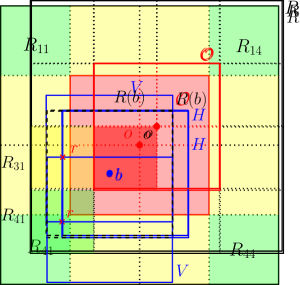
  (a)

  

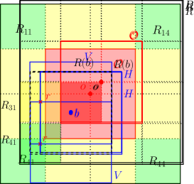
  (b)

  Figure 21: ${\cal O}$ (red) is an optimum square centered at a point $o$, and $R$ (black) is a square of length 2 centered at $o$. $R(b)$ is the square centered at a blue point $b\in{\cal O}_{SW}$. The squares $H$ and $V$ are the horizontal and the vertical translated copies of $R(b)$, respectively. (a) The red point $r$ lies in a corner sub-square $R_{41}$ of $R$. (b) The red point $r$ lies in a side sub-square $R_{31}$ of $R$.

• Case 3: The red point $r$ lies in a side sub-square of $R$ (see Figure 21(b)). W.l.o.g., assume that $r\in R_{31}$; the other cases are similar. Now, if $b$ lies in ${\cal O}_{SW}=R_{32}$ or in ${\cal O}_{NW}=R_{22}$, then the square $R(b)$ may contain $r$. Suppose, $b\in{\cal O}_{SW}$. If $r\notin R(b)$, then ${\mathcal{S}}(b)=\{R(b)\}$ and clearly ${\cal O}_{SW}\subseteq R(b)$. Otherwise, $r\in R(b)$. In that case, again as defined in Section 4.3 (Case 4), there are exactly two (non-empty) candidate squares of $b$, and it is easy to see that one of them must contain ${\cal O}_{SW}$. Similarly, if $b\in{\cal O}_{NW}$, we can show that $b$ has at most two (non-empty) candidate squares, and one of them must contain ${\cal O}_{NW}$. Now, consider that $b\in{\cal O}_{NE}\cup{\cal O}_{SE}$. In this case, observe that $R(b)$ never contains $r$. As a result, ${\mathcal{S}}(b)=\{R(b)\}$, and $R(b)$ contains the sub-square of ${\cal O}$, where $b$ lies (due to Observation 1). Therefore, Algorithm 3 needs at most $6$ candidate squares to cover all the blue points in ${\cal O}$.

Hence, the lemma follows.

∎

Theorem 2.

There exists an algorithm for the online class cover problem for squares that achieves a competitive ratio of $\max\{6,20\log_{2}(m)\}$, where $m\ (\geq 0)$ is the number of red points.

Proof.

Let ${\cal I}$ be an input sequence of blue points. Suppose that $\text{OPT}({\cal I})$ be an optimal solution given by an offline algorithm, and $\text{ALG}({\cal I})$ be the solution given by Algorithm 3 for the sequence ${\cal I}$. Also, let ${\cal O}\in\text{OPT}({\cal I})$. Consider first that $m=0$, i.e. there are no red points. Whenever a blue point, say $u$, is introduced to the algorithm and not already covered by the previously selected squares, Algorithm 3 places $R(u)$ to cover $u$. As a result of Observation 1, we have that Algorithm 3 needs at most $4$ squares to cover all the blue points of ${\cal I}\cap{\cal O}$. Therefore, $|\text{ALG}({\cal I})|\leq\sum_{{\cal O}\in\text{OPT}({\cal I})}4=4|\text{OPT}({\cal I})|$.

Now, consider that $m=1$, i.e. there is exactly one red point. From Lemma 4, we have that Algorithm 3 needs at most $6$ squares to cover all the blue points of ${\cal I}\cap{\cal O}$. Therefore, $|\text{ALG}({\cal I})|\leq\sum_{{\cal O}\in\text{OPT}({\cal I})}6=6|\text{OPT}({\cal I})|$.

Next, we consider $m\geq 2$. From Lemma 3, we have that Algorithm 3 needs at most $20\log_{2}(m)$ squares to cover all the blue points of ${\cal I}\cap{\cal O}$. Therefore, $|\text{ALG}({\cal I})|\leq\sum_{{\cal O}\in\text{OPT}({\cal I})}20\log_{2}(m)=20\log_{2}(m)|\text{OPT}({\cal I})|$. Thus, the theorem follows. ∎

5.3 Improving the Competitive Ratio Further

Note that in Lemma 2, we have proved that if $u\in{\cal O}_{SW}$ such that any candidate squares of $u$ does not contain ${\cal O}_{SW}$, then their union contains ${\cal O}_{NW}\cup{\cal O}_{SE}$. The equivalent statement is true when $u$ lies in other sub-squares of ${\cal O}$. So, a careful analysis of Algorithm 3 reduces the competitive ratio to $10+10\log_{2}(m)$ from $20\log_{2}(m)$, where $m\ (\geq 2)$ is the number of red points (see Figure 22). Let $u_{1},u_{2},\dots,u_{k}$ be the largest sub-sequence of the input sequence such that $u_{i}\in{\cal O}$ for $i\in[k]$, and they are uncovered upon arrival. W.l.o.g., we assume that $u_{1}\in{\cal O}_{SW}$. So due to Lemma 1, we have the following two cases.

Figure 22: Red square is an optimum square. Blue points are the input points. Some candidate squares cover green-shaded regions.

1. A candidate square of $u_{1}$ contains ${\cal O}_{SW}$. Hence, next blue point $u_{2}$ lies on either ${\cal O}_{NW}\cup{\cal O}_{SE}$ or ${\cal O}_{NE}$.

   1. Let $u_{2}$ lies on ${\cal O}_{NW}\cup{\cal O}_{SE}$. W.l.o.g., assume that $u_{2}\in{\cal O}_{NW}$. The other case is similar. Then due to Lemma 1, we have the following two cases.

      1. A candidate square of $u_{2}$ contains ${\cal O}_{NW}$. In this case, Algorithm 3 needs at most $2\cdot 5\log_{2}(m)$ candidate squares to cover ${\cal O}_{NE}\cup{\cal O}_{SE}$ (due to Lemma 2). Therefore, our algorithm needs at most $10+10\log_{2}(m)$ candidate squares to cover ${\cal O}$.

      2. Union of the candidate squares of $u_{2}$ contains ${\cal O}_{NE}\cup{\cal O}_{SW}$. In this case, Algorithm 3 needs at most $2\cdot 5\log_{2}(m)$ candidate squares to cover ${\cal O}_{NW}\cup{\cal O}_{SE}$ (due to Lemma 2). Therefore, our algorithm needs at most $10+10\log_{2}(m)$ candidate squares to cover ${\cal O}$.

   2. Let $u_{2}$ lies ${\cal O}_{NE}$. Then due to Lemma 1, we have the following two cases.

      1. A candidate square of $u_{2}$ contains ${\cal O}_{NE}$. In this case, Algorithm 3 needs at most $2\cdot 5\log_{2}(m)$ candidate squares to cover ${\cal O}_{NW}\cup{\cal O}_{SE}$ (due to Lemma 2). Therefore, our algorithm needs at most $10+10\log_{2}(m)$ candidate squares to cover ${\cal O}$.

      2. Union of the candidate squares of $u_{2}$ contains ${\cal O}_{NW}\cup{\cal O}_{SE}$. In this case, Algorithm 3 needs at most $5\log_{2}(m)$ candidate squares to cover ${\cal O}_{NE}$ (due to Lemma 2). Therefore, our algorithm needs at most $10+5\log_{2}(m)$ candidate squares to cover ${\cal O}$.

2. Union of the candidate squares of $u_{1}$ contains ${\cal O}_{NW}\cup{\cal O}_{SE}$. In this case, Algorithm 3 needs at most $2\cdot 5\log_{2}(m)$ candidate squares to cover ${\cal O}_{SW}\cup{\cal O}_{NE}$ (due to Lemma 2). Therefore, our algorithm needs at most $5+10\log_{2}(m)$ candidate squares to cover ${\cal O}$.

Hence, we have the following theorem.

Theorem 3.

There exists an algorithm for the online class cover problem for squares that achieves a competitive ratio of $\max\{6,10+10\log_{2}(m)\}$, where $m\ (\geq 0)$ is the number of red points.

6 Translated Copies of a Rectangle

In this section, we consider the online class cover problem for translated copies of a rectangle and prove that the upper bound of $O(\log m)$ is also applicable. Let $R=\square abcd$ be a rectangle in a plane (see Figure 23). Let $p,q,r$ and $s$ be the midpoints of the edges $ab,bc,cd$ and $ad$ of $R$, respectively. Then, the centre of the rectangle $R$ is defined to be the intersection point of the line segments $\overline{pr}$ and $\overline{qs}$. Also, the two line segments $\overline{pr}$ and $\overline{qs}$ partition $R$ into four smaller rectangles, called sub-rectangles. Now, observe that the equivalent result of Observation 1 holds when the objects are translated copies of a rectangle.

Observation 3.

Let $u$ be any blue point and $P$ be any rectangle such that $u\in P$. Then, $P$ must contain at least one of the sub-rectangles of $R$, where $R$ is a translated copy of $P$ centered at $u$.

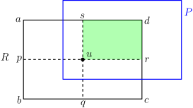
Figure 23: $R$ (black) is a rectangle centered at $u$. Now, $P$ (blue) is a translated copy of $R$ containing $u$. Note that $P$ also contains the $NE$ sub-rectangle (green shaded) of $R$.

Due to this, we can define the candidate rectangles of a blue point similarly as we defined the candidate squares in Section 4.3. Also, we can prove the competitive ratio of the Algorithm 3 to be $O(\log m)$ in a similar way as shown in Section 5.2. Thus, we have the following theorem.

Theorem 4.

An algorithm for the online class cover problem exists for translated copies of a rectangle that achieves an optimal competitive ratio of $O(\log m)$, where $m$ is the number of red points.

7 Conclusion

In this paper, we have discussed the online class cover problem. Our main results are proofs for a lower and upper bound of the problem for axis-parallel unit squares. We also proved that the upper bound applies to the problem even if the geometric objects are translated copies of a rectangle. Notice that the lower and upper bound of the problem depends on the maximum number of red points that can lie in a rectangle. If this number is bounded by a constant, then so are the lower and upper bounds of the problem. Obtaining the same bounds for unit disks or translates of a convex object will be an interesting question. Since our algorithm and lower bound are on the deterministic model, it would be important to question whether randomization helps to obtain a better competitive ratio.

Conflict of Interest

The authors declare that there are no financial and non-financial competing interests that are relevant to the content of this article.

References

- [1] Pankaj K. Agarwal and Subhash Suri. Surface approximation and geometric partitions. SIAM J. Comput., 27(4):1016–1035, 1998.
- [2] Noga Alon, Baruch Awerbuch, Yossi Azar, Niv Buchbinder, and Joseph Naor. The online set cover problem. SIAM J. Comput., 39(2):361–370, 2009.
- [3] Rom Aschner, Matthew J. Katz, Gila Morgenstern, and Yelena Yuditsky. Approximation schemes for covering and packing. In Subir Kumar Ghosh and Takeshi Tokuyama, editors, WALCOM: Algorithms and Computation, 7th International Workshop, WALCOM 2013, Kharagpur, India, February 14-16, 2013. Proceedings, volume 7748 of Lecture Notes in Computer Science, pages 89–100. Springer, 2013.
- [4] Sergey Bereg, Sergio Cabello, José Miguel Díaz-Báñez, Pablo Pérez-Lantero, Carlos Seara, and Inmaculada Ventura. The class cover problem with boxes. Comput. Geom., 45(7):294–304, 2012.
- [5] Allan Borodin and Ran El-Yaniv. Online computation and competitive analysis. Cambridge University Press, 1998.
- [6] Adam Cannon and Lenore Cowen. Approximation algorithms for the class cover problem. Ann. Math. Artif. Intell., 40(3-4):215–224, 2004.
- [7] Adam H Cannon, Lenore J Cowen, and Carey E Priebe. Approximate distance classification. Computing Science and Statistics, pages 544–549, 1998.
- [8] Ioannis Caragiannis, Aleksei V. Fishkin, Christos Kaklamanis, and Evi Papaioannou. Randomized on-line algorithms and lower bounds for computing large independent sets in disk graphs. Discret. Appl. Math., 155(2):119–136, 2007.
- [9] Jean Cardinal, Justin Dallant, and John Iacono. Approximability of (simultaneous) class cover for boxes. In Meng He and Don Sheehy, editors, Proceedings of the 33rd Canadian Conference on Computational Geometry, CCCG 2021, August 10-12, 2021, Dalhousie University, Halifax, Nova Scotia, Canada, pages 149–156, 2021.
- [10] Timothy M. Chan and Hamid Zarrabi-Zadeh. A randomized algorithm for online unit clustering. Theory Comput. Syst., 45(3):486–496, 2009.
- [11] Moses Charikar, Chandra Chekuri, Tomás Feder, and Rajeev Motwani. Incremental clustering and dynamic information retrieval. SIAM J. Comput., 33(6):1417–1440, 2004.
- [12] Ke Chen, Amos Fiat, Haim Kaplan, Meital Levy, Jirí Matousek, Elchanan Mossel, János Pach, Micha Sharir, Shakhar Smorodinsky, Uli Wagner, and Emo Welzl. Online conflict-free coloring for intervals. SIAM J. Comput., 36(5):1342–1359, 2007.
- [13] Ke Chen, Haim Kaplan, and Micha Sharir. Online conflict-free coloring for halfplanes, congruent disks, and axis-parallel rectangles. ACM Trans. Algorithms, 5(2):16:1–16:24, 2009.
- [14] Lenore J Cowen and Carey E Priebe. Randomized nonlinear projections uncover high-dimensional structure. Advances in Applied Mathematics, 19(3):319–331, 1997.
- [15] Minati De, Saksham Jain, Sarat Varma Kallepalli, and Satyam Singh. Online piercing of geometric objects. In Anuj Dawar and Venkatesan Guruswami, editors, 42nd IARCS Annual Conference on Foundations of Software Technology and Theoretical Computer Science, FSTTCS 2022, December 18-20, 2022, IIT Madras, Chennai, India, volume 250 of LIPIcs, pages 17:1–17:16. Schloss Dagstuhl - Leibniz-Zentrum für Informatik, 2022.
- [16] Minati De, Sambhav Khurana, and Satyam Singh. Online dominating set and independent set. CoRR, abs/2111.07812, 2021.
- [17] Minati De and Satyam Singh. Hitting geometric objects online via points in $\mathbb {Z}^d$. In Yong Zhang, Dongjing Miao, and Rolf H. Möhring, editors, Computing and Combinatorics - 28th International Conference, COCOON 2022, Shenzhen, China, October 22-24, 2022, Proceedings, volume 13595 of Lecture Notes in Computer Science, pages 537–548. Springer, 2022.
- [18] Jason Gary DeVinney. The class cover problem and its applications in pattern recognition. Ph.D. dissertation, The Johns Hopkins University, 2003.
- [19] Adrian Dumitrescu, Anirban Ghosh, and Csaba D. Tóth. Online unit covering in Euclidean space. Theor. Comput. Sci., 809:218–230, 2020.
- [20] Adrian Dumitrescu and Csaba D. Tóth. Online unit clustering and unit covering in higher dimensions. Algorithmica, 84(5):1213–1231, 2022.
- [21] Stephan Eidenbenz. Online dominating set and variations on restricted graph classes. Technical Report No 380, ETH Library, 2002.
- [22] Guy Even and Shakhar Smorodinsky. Hitting sets online and unique-max coloring. Discret. Appl. Math., 178:71–82, 2014.
- [23] Oliver Göbel, Martin Hoefer, Thomas Kesselheim, Thomas Schleiden, and Berthold Vöcking. Online independent set beyond the worst-case: Secretaries, prophets, and periods. In Javier Esparza, Pierre Fraigniaud, Thore Husfeldt, and Elias Koutsoupias, editors, Automata, Languages, and Programming - 41st International Colloquium, ICALP 2014, Copenhagen, Denmark, July 8-11, 2014, Proceedings, Part II, volume 8573 of Lecture Notes in Computer Science, pages 508–519. Springer, 2014.
- [24] Arindam Khan, Aditya Lonkar, Saladi Rahul, Aditya Subramanian, and Andreas Wiese. Online and dynamic algorithms for geometric set cover and hitting set. In Erin W. Chambers and Joachim Gudmundsson, editors, 39th International Symposium on Computational Geometry, SoCG 2023, June 12-15, 2023, Dallas, Texas, USA, volume 258 of LIPIcs, pages 46:1–46:17. Schloss Dagstuhl - Leibniz-Zentrum für Informatik, 2023.
- [25] Joseph SB Mitchell. Approximation algorithms for geometric separation problems. Technical report, AMS Dept., SUNY Stony Brook, NY, 1993.
- [26] Sima Hajiaghaei Shanjani. Hardness of approximation for red-blue covering. In J. Mark Keil and Debajyoti Mondal, editors, Proceedings of the 32nd Canadian Conference on Computational Geometry, CCCG 2020, August 5-7, 2020, University of Saskatchewan, Saskatoon, Saskatchewan, Canada, pages 39–48, 2020.