A simple construction of Entanglement Witnesses for arbitrary and different dimensions

Abstract

We present a simple approach for generation of a diverse set of positive maps between spaces of different dimensions. The proposed method enables the construction of Entanglement Witnesses tailored for systems in $d_{1}\times d_{2}$ dimensions. With this method, it is possible to construct Entanglement Witnesses that consist solely of a chosen set of desired measurements. We demonstrate the effectiveness and generality of our approach using concrete examples. It is also demonstrated in two examples, how an appropriate entanglement witness can be identified for witnessing the entanglement of a given state, including a case when the given state is a Positive Partial Transpose (PPT) entangled state.

Introduction

Entanglement stands out as one of the most remarkable distinctions between the quantum and classical realms, playing a pivotal role in numerous quantum protocols, for review papers see [1, 2, 3]. As a result, the creation, manipulation, application, and identification of entanglement have profound significance. The identification of entangled states, in particular, presents a formidable challenge, underscored by its classification as an NP-Hard problem in mathematical terms [4]. Hence, the pursuit of viable techniques for detecting entangled states takes on paramount importance.

Entangled states are referred to as states that are not separable, and separable states refer to states that can be written as follows[5]:

$$\rho=\sum p_{i}\rho_{i}^{(1)}\otimes\rho_{i}^{(2)},$$ (1)

where $0\leq p_{i}\leq 1$ and $\sum p_{i}=1$. One strategy for identifying entanglement involves investigating whether a state can be expressed in the aforementioned form. This, however, poses a formidable challenge. As a result, there is a pressing need for more effective methodologies for the detection of entanglement. Over time, diverse techniques have emerged for this purpose. The Peres criterion is considered one of the primary methods in this regard[6]: It’s relatively straightforward to see that the partial transpose of all separable states is positive. This is seen simply by noting that for any state of the form (1), one has

$$(I\otimes T)(\rho)\geq 0,$$ (2)

where $T$ is the transpose, hence the name partial transpose. Therefore, if the partial transpose of a quantum state is not positive, it must be entangled. However, this criterion alone cannot identify all types of quantum entangled states because there are entangled states known as PPT, whose partial transpose are positive. In fact separable states are a subset of PPT states and only when $d_{1}d_{2}\leq 6$, these two sets are equal. Here $d_{1}$ and $d_{2}$ are the dimensions of the two quantum systems. The effectiveness of the Peres criteria (2) hinges on a basic property of the transpose map $T$ which is a positive and yet not completely positive map. Therefore it was natural to search for more general types of positive maps lacking the property of complete positivity and thus constructing more general Entanglement Witnesses than the simple partial transpose. In fact, it has been known that any entanglement witness $W$ can be written in the form

$$W(M)=(I\otimes M)|\phi^{+}\rangle\langle\phi^{+}|,$$ (3)

where $M$ is a positive map and $|\phi^{+}\rangle=\frac{1}{\sqrt{d}}\sum_{\mu=0}^{d-1}|\mu\mu\rangle$, is a maximally entangled state. In other words, $W(M)$ is the Choi-matrix of the map $M$, which due to its lack of complete positivity can have negative eigenvalue. Such a witness has the property

$$\operatorname{Tr}(W\sigma)\geq 0,\quad\forall\sigma\in S,$$ (4)

where $S$ is the set of all separable states. Alternatively, one can think of $W$ as a block-positive operator, i.e.

$$\langle\psi,\phi|W|\psi,\phi\rangle,\ \forall\ \psi\in H_{1}\ ,\forall\ \phi\in H_{2},$$

which has negative eigenvalue when acting on the whole Hilbert space $H_{1}\otimes H_{2}$. Thus the problem of constructing entanglement witnesses becomes equivalent to constructing positive but not completely positive maps. Based on this equivalence, entanglement witnesses were introduced in many works, see [7, 8, 9, 10] and references therein. For more recent works, see [11, 12, 13]. In practical situations, where the two particles are far apart in remote laboratories, application of any entanglement witnesses found so far, requires a common reference frame between the two parties holding the particles. It was recently shown in [14] that by a process called incomplete teleportation, all these entangled states are still able to detect entanglement of remote parties, even in the absence of a common frame of reference.

In contrast with completely positive maps which due to the Kraus theorem can be easily constructed, construction of positive maps is not a straightforward task, and appropriate methods need to be proposed for this purpose. In addition to the finding new classes of witnesses, the relation of EW’s and positive maps, have led to many new insights on both [8]. For example, a basic distinction refers to decomposable witnesses which are of the form

$$W=P+Q^{\Gamma},$$

where $P,Q$ are positive operators and $\Gamma$ is the operator of partial transposition. Any witness that cannot be written in the above form is called indecomposable. It can be proved that decomposable witnesses cannot identify PPT states. In this sense these are somewhat weaker than indecomposable witnesses. One can also characterize witnesses by their optimality and extremality [8], a subject which we will not deal with in this work. The line that we follow is inspired by a number of recent works [15, 16, 17, 18, 19, 20] in which specific types of positive maps have been defined and the corresponding witnesses have been constructed.

It is worth noting that in all mentioned articles, the entanglement witnesses constructed have been designed for two systems of equal dimensions. In this paper, we propose a simple method for identification of entanglement in systems with dimensions of $d_{1}\times d_{2}$. This dimension-specific applicability enhances the versatility of the method, making it a valuable tool in different practical scenarios. Often, due to practical constraints in laboratory setups, certain measurements may be more accessible or accurate than others. Our method elegantly accommodates this by allowing for the construction of entanglement witnesses based solely on those restricted measurements which are feasible in the given experimental context(See examples).

The structure of this paper is as follows: In Section 1, we examine the main idea of this article, which is to construct a new class of positive maps. In Section 2, an alternative method is utilized to obtain the same results that presented in Section 1. In section 3, we employ singular value decomposition to simplify the presentation of the obtained results. In Section 4, we present several examples each of which elaborate one particular advantage of this construction. Finally, in section 5, we demonstrate how one can construct entanglement witnesses for an arbitrary state using the method described in this paper. We end up the paper with a conclusion.

1 Construction of positive maps for arbitrary different dimensions

Consider the Hilbert space $H_{d_{1}}$ of dimension $d_{1}$ and let a pure state $X\in D(H_{d_{1}})$, (the space of states on $H_{d_{1}}$) be written as

$$X=\frac{1}{d_{1}}\mathcal{I}_{d_{1}}+\sum_{i=1}^{d_{1}^{2}-1}x_{i}\Gamma_{i},$$ (5)

where $\{\Gamma_{i},\ \ \ i=1\cdots d_{1}^{2}-1\}$ are a set of orthonormal traceless Hermitian operators $\in L(H_{d_{1}})$, i.e.

$$\operatorname{Tr}(\Gamma_{i}\Gamma_{j})=\delta_{ij},\ \ \ \operatorname{Tr}\Gamma_{i}=0.$$ (6)

Purity of the state $X$ (i.e. $\operatorname{Tr}X^{2}=1$) and the above normalization conditions restricts the norm of the vector ${\bf x}=(x_{1},\cdots x_{d_{1}^{2}-1})$ to

$${\bf x}\cdot{\bf x}=\frac{d_{1}-1}{d_{1}},$$ (7)

where ${\bf x}\cdot{\bf x}:=\sum_{i=1}^{d_{1}^{2}-1}x_{i}^{2}$.

Let $\Phi:D(H_{d_{1}})\longrightarrow D(H_{d_{2}})$ be unital and trace-preserving map which acts as follows:

$$\Phi(\frac{1}{d_{1}}\mathcal{I}_{d_{1}})=\frac{1}{d_{2}}\mathcal{I}_{d_{2}}\ \ \ \ ,\ \ \ \Phi(\Gamma_{i})=\frac{1}{d_{2}}\sum_{k=1}^{d_{2}^{2}-1}\Lambda_{ik}\Omega_{k}.$$ (8)

In fact, $\Lambda_{ik}$ are real numbers representing the characterization of the map $\Phi$. Here, our definition remains consistent with the trace-preserving property of the map, in contrast to the definition presented in [18], which is grounded in the property of such a map that takes an identity matrix in $D(H_{d_{1}})$ to a identity matrix in $D(H_{d_{2}})$. The factor $\frac{1}{d_{2}}$ in the second equation is written for later convenience, and $\{\Omega_{k},\ \ \ k=1\cdots d_{2}^{2}-1\}$ are a set of orthonormal traceless Hermitian operators $\in L(H_{d_{2}})$, i.e.

$$\operatorname{Tr}(\Omega_{k}\Omega_{l})=\delta_{kl},\ \ \ \operatorname{Tr}\Omega_{k}=0.$$ (9)

Then $\Phi$ maps $X$ to

$$\Phi(X)=\frac{1}{d_{2}}\mathcal{I}_{d_{2}}+\frac{1}{d_{2}}\sum_{i=1}^{d_{1}^{2}-1}\sum_{k=1}^{d_{2}^{2}-1}x_{i}\Lambda_{ik}\Omega_{k}.$$ (10)

Remark 1

Up to now we have assumed that $X$ is a pure state. This can be extended to arbitrary operatores $X\in L(H_{d})$ as follows:

$$\Phi(X)=\frac{\operatorname{Tr}(X)}{d_{2}}\mathcal{I}_{d_{2}}+\frac{1}{d_{2}}\sum_{i=1}^{d_{1}^{2}-1}\sum_{k=1}^{d_{2}^{2}-1}x_{i}\Lambda_{ik}\Omega_{k}.$$ (11)

To ensure positivity of the map $\Phi$, we now use Mehta’s Lemma [21] which we state below:

Mehta’s Lamma (1989): Let $A$ be a Hermitian matrix of dimension $D$, if

$$\operatorname{Tr}(A^{2})\leq\frac{(\operatorname{Tr}A)^{2}}{D-1},$$ (12)

then $A$ is positive.

In view of linearity of the map $\Phi$, to prove positivity of the map $\Phi$, it is sufficient to prove that $\Phi(X)$ is positive for any pure state $X$. That is the map $\Phi$ is positive if the following condition holds

$$\operatorname{Tr}(\Phi(X)^{2})\leq\frac{(\operatorname{Tr}\Phi(X))^{2}}{d_{2}-1}=\frac{1}{d_{2}-1}.$$ (13)

To this end, we calculate $\operatorname{Tr}(\Phi(X)^{2})$, which in view of orthonormality condition (8), turns out to be

$$\operatorname{Tr}(\Phi(X)^{2})=\frac{1}{d_{2}}+\frac{1}{d_{2}^{2}}{\bf x}^{T}{\Lambda}\Lambda^{T}{\bf x},$$ (14)

where the matrix $\Lambda$ is composed of $\Lambda_{ij}$ elements. In view of (12), we demand that

$$\frac{1}{d_{2}}+\frac{1}{d_{2}^{2}}{\bf x}^{T}{\Lambda}\Lambda^{T}{\bf x}\leq\frac{1}{d_{2}-1},\hskip 28.45274pt\forall{\bf x}.$$ (15)

We can now replace this with an even stronger inequality, namely

$$\frac{1}{d_{2}}+\frac{1}{d_{2}^{2}}\lambda_{max}(\Lambda{\Lambda^{T}}){\bf x}\cdot{\bf x}\leq\frac{1}{d_{2}-1},$$ (16)

where $\lambda_{max}:=\lambda_{max}(\Lambda\Lambda^{T})$, is the largest eigenvalue of the matrix $\Lambda\Lambda^{T}$, or equivalently $\lambda_{max}$ is the square of the largest singular value of the matrix $\Lambda^{T}$. Inserting (16) in (13), yields the following constraint on $\lambda_{max}$

$$\lambda_{max}\leq\frac{d_{1}d_{2}}{(d_{1}-1)(d_{2}-1)}.$$ (17)

The EW corresponding to the map (10) is given by [7]

$$W=(\mathcal{I}_{d_{1}}\otimes\Phi)|\beta\rangle\langle\beta|,$$ (18)

where $|\beta\rangle=\frac{1}{\sqrt{d}}\sum_{\mu=0}^{d_{1}-1}|\mu,\mu\rangle$ is a maximally entangled state. To do this calculation, we extend the orthonormal sets $\{\Gamma_{i}\}$ and $\{\Omega_{k}\}$ respectively to orthonormal bases for the space of matrices $M_{d_{1}}$ and $M_{d_{2}}$, namely to $\{\Gamma_{\mu}\}=\{\Gamma_{0}=\frac{\mathcal{I}}{\sqrt{d_{1}}},\Gamma_{i}\}$ and $\{\Omega_{\mu}\}=\{\Omega_{0}=\frac{\mathcal{I}}{\sqrt{d_{2}}},\Omega_{i}\}$ and taking remark 1 into account, we write

$$W = \frac{1}{d_{1}}\sum_{\mu,\nu}|\mu\rangle\langle\nu|\otimes\Phi(|\mu\rangle\langle\nu|)$$ (19)

$$= \frac{1}{d_{1}}\sum_{\mu,\nu}|\mu\rangle\langle\nu|\otimes\sum_{\beta}\Lambda_{\beta\alpha}\operatorname{Tr}(|\mu\rangle\langle\nu|\Gamma_{\beta})\Omega_{\alpha}$$ (20)

$$= \frac{1}{d_{1}}\sum_{\alpha,\beta}\Lambda_{\beta\alpha}\Gamma^{T}_{\beta}\otimes\Omega_{\alpha}.$$ (21)

After multiplication by an overall factor $d_{1}d_{2}$, this leads to the following witness

$$W=\mathcal{I}_{d_{1}}\otimes\mathcal{I}_{d_{2}}+\sum_{i=1}^{d_{1}^{2}-1}\sum_{k=1}^{d_{2}^{2}-1}{\Lambda}_{ik}\Gamma^{T}_{i}\otimes\Omega_{k}.$$ (22)

Since the set $\Gamma^{T}_{i}$ is also an orthonormal set, we can rename it to $\Gamma_{i}$. Thus, the following matrix can be a entanglement witness too:

$$W=\mathcal{I}_{d_{1}}\otimes\mathcal{I}_{d_{2}}+\sum_{i=1}^{d_{1}^{2}-1}\sum_{k=1}^{d_{2}^{2}-1}{\Lambda}_{ik}\Gamma_{i}\otimes\Omega_{k}.$$ (23)

Therefore for any two dimensions, any operator of the above form can be an entanglement witness, provided that the condition (17) holds. That condition in fact proves Block positivity of this Witness. Whether or not a $W$ constructed in this way, has also a negative eigenvalue depends on the matrix $\Lambda$ that we choose. In all previous papers that were mentioned in the introduction, $\Lambda$ should be orthogonal. These comprise a much smaller class compared to the $\Lambda$ matrices in this paper. Moreover, finding orthogonal matrices in high dimensions is not a straightforward task. In this paper, one can use any matrix with any properties to construct entanglement witnesses, as long as the largest eigenvalue of $\Lambda\Lambda^{T}$ satisfies eq. (17). Furthermore, to demonstrate the efficacy of the proposed method, we presented an algorithmic approach in section (5), which enables the straightforward construction of entanglement witnesses for desired states.

In the next section, we derive the same result of eq. (23) in an alternative way by focusing on the EW itself, rather than the positive map which leads to it via its Choi-matrix. In view of this alternative construction, one can first choose the local operators (according to the experimental restrictions) and then tuning the coefficients for defining the final entanglement witness. This is a significant advantage compared to methods where a positive map may lead to a witness which requires non-feasible measurements.

2 An alternative construction of Entanglement Witnesses

In this section we directly apply Mehta’s Lemma to a form of EW which we take as follows:

$$W=I_{d_{1}}\otimes I_{d_{2}}+\sum_{i=1}^{d_{1}^{2}-1}\sum_{j=1}^{d_{2}^{2}-1}\Lambda_{ij}\Gamma_{i}\otimes\Omega_{j}.$$ (24)

We demand that $W$ be block-positive. This means that for any vector $|v\rangle\in H_{d_{2}}$, the following matrix should be positive

$$B\equiv\langle v|W|v\rangle=I_{d_{1}}+\sum_{i=1}^{d_{1}^{2}-1}\sum_{j=1}^{d_{2}^{2}-1}\Lambda_{ij}\Gamma_{i}\langle v|\Omega_{j}|v\rangle.$$ (25)

Now we use the following:

$$\operatorname{Tr}(B)=d_{1},$$ (26)

and

$$\operatorname{Tr}(B^{2})=d_{1}+\sum_{i,j=1}^{d_{2}^{2}-1}(\Lambda^{T}\Lambda)_{ij}\langle v|\Omega_{i}|v\rangle\langle v|\Omega_{j}|v\rangle,$$ (27)

where we have used the relations $\operatorname{Tr}(\Gamma_{i})=0,\ \ \ \operatorname{Tr}(\Gamma_{i}\Gamma_{j})=\delta_{ij}$. We now resort to the Mehta’s Lemma and demand that the following condition hold for all the vectors $|v\rangle$

$$\operatorname{Tr}(B^{2})\leq\frac{\operatorname{Tr}(B)^{2}}{d_{1}-1}.$$ (28)

This leads to

$$d_{1}+\sum_{i,j=1}^{d_{2}^{2}-1}(\Lambda^{T}\Lambda)_{ij}\langle v|\Omega_{i}|v\rangle\langle v|\Omega_{j}|v\rangle\leq\frac{d_{1}^{2}}{d_{1}-1}\hskip 28.45274pt\forall\ v.$$ (29)

Defining the vector ${\bf q}$ with components $q_{i}:=\langle v|\Omega_{i}|v\rangle$, this can be written as

$$d_{1}+{\bf q}^{T}\Lambda\Lambda^{T}{\bf q}\leq\frac{d_{1}^{2}}{d_{1}-1}\hskip 28.45274pt\forall\ v,$$ (30)

or in a stronger form

$$d_{1}+\lambda_{max}(\Lambda^{T}\Lambda){\bf q}.{\bf q}\leq\frac{d_{1}^{2}}{d_{1}-1}.$$ (31)

It remains to calculate ${\bf q}.{\bf q}$, and this is easily found by noting that

$${\bf q}.{\bf q}=\sum_{i=1}^{d_{2}^{2}-1}\langle v|\Omega_{i}|v\rangle\langle v|\Omega_{i}|v\rangle=\sum_{i=1}^{d_{2}^{2}-1}\langle v,v|\Omega_{i}\otimes\Omega_{i}|v,v\rangle.$$

Using the identity

$$\frac{1}{d}\mathcal{I}+\sum_{i}\Omega_{i}\otimes\Omega_{i}=P,$$ (32)

where $P$ is the permutation operator (look at appendix A for the proof of this equation). We find that

$${\bf q}.{\bf q}=\langle v,v|P-\frac{1}{d_{2}}\mathcal{I}|v,v\rangle=1-\frac{1}{d_{2}}.$$ (33)

Inserting this in (31), leads to the final form for the upper bound of $\lambda_{max}$, namely

$$\lambda_{max}(\Lambda^{T}\Lambda)\leq\frac{d_{1}d_{2}}{(d_{1}-1)(d_{2}-1)},$$ (34)

which is identical to the bound obtained by the positive map in section 1. However we should also ensure that $W$ is not trivially positive, that is we should remove the possibility that all its eigenvalues be positive. We again use Mehta’s lemma. To this end we use

$$\operatorname{Tr}(W)=d_{1}d_{2},$$ (35)

and

$$\operatorname{Tr}(W^{2})=d_{1}d_{2}+\operatorname{Tr}(\Lambda^{T}\Lambda),$$ (36)

and ensure that the following inequality be satisfied

$$\operatorname{Tr}(W^{2})>\frac{\operatorname{Tr}(W)^{2}}{d_{1}d_{2}-1},$$ (37)

or

$$\frac{d_{1}d_{2}}{d_{1}d_{2}-1}<\operatorname{Tr}(\Lambda^{T}\Lambda).$$ (38)

Combining (34) and (38), we arrive at the final condition for the parameters of the matrix $\Lambda$, in order that $W$ can be an entanglement witness:

$$\frac{d_{1}d_{2}}{d_{1}d_{2}-1}<\operatorname{Tr}(\Lambda^{T}\Lambda),\ \ \ \ {\rm and}\ \ \ \lambda_{max}\leq\frac{d_{1}d_{2}}{(d_{1}-1)(d_{2}-1)}.$$ (39)

Note that the second condition is sufficient for the block-positivity of $W$, while the first condition is necessary for $W$, ensuring that it is not a positive matrix.

3 Singular value decomposition of $\Lambda$

The matrix $\Lambda$ can be singular-value decomposed in the form $\Lambda=RDS$, where $R$ and $S$ are orthogonal matrices, $R\in\textrm{SO}(d_{1}^{2}-1)$ and $S\in\textrm{SO}(d_{2}^{2}-1)$ and $D$ is a diagonal matrix consisting of real values $\{c_{1},c_{2},\cdots\}$ on its main diagonal. This decomposition allows us to write $W$ in the form

$$W=\mathcal{I}_{d_{1}}\otimes\mathcal{I}_{d_{2}}+\sum_{i=1}^{min(d_{1}^{2}-1,d_{2}^{2}-1)}c_{i}\Gamma^{\prime}_{i}\otimes\Omega^{\prime}_{i},$$ (40)

where $\Gamma^{\prime}_{i}=\sum_{j=1}^{d_{1}^{2}-1}R_{ij}\Gamma_{j}$ and $\Omega^{\prime}_{i}=\sum_{m=1}^{d_{2}^{2}-1}S_{im}\Omega_{m}$ are new orthonormal bases. Hereafter we work with these new bases (or assume that off-diagonal elements of $\Lambda$ are zero from the very beginning). Hence, for the sake of simplicity, as $\Omega^{\prime}_{i}$ and $\Gamma_{i}^{\prime}$ are new orthonormal bases, we can rename them as $\Omega_{i}$ and $\Gamma_{i}$, respectively, and write $W$ as

$$W=\mathcal{I}_{d_{1}}\otimes\mathcal{I}_{d_{2}}+\sum_{i=1}^{min(d_{1}^{2}-1,d_{2}^{2}-1)}c_{i}\Gamma_{i}\otimes\Omega_{i},$$ (41)

where according to (39), the coefficients $c_{i}$ are subject to the following condition

$$\frac{d_{1}d_{2}}{d_{1}d_{2}-1}<\sum_{i=1}c_{i}^{2}\ \ \ \ {\rm and}\ \ \ \ c_{max}^{2}\leq{\frac{d_{1}d_{2}}{(d_{1}-1)(d_{2}-1)}}.$$ (42)

Remark 2

It should be noted that for each basis of orthonormal operators that we choose in (41), we obtain a different EW, even if the coefficients $c_{i}$ are identical. Only in the special case of $d_{1}=d_{2}=2$, the EW is entirely characterized by the parameters $c_{i}$. This is due to the fact that in two dimensions, we can use the isomorphism $SU(2)\sim SO(3)$ to implement the transformations

$$U\Gamma_{i}U^{\dagger}=\Gamma^{\prime}_{i},\hskip 28.45274ptV\Omega_{i}V^{\dagger}=\Omega_{i}^{\prime},\quad\forall\ \ i,$$ (43)

and prove that an EW can always be put into the canonical form $W_{c}$ by the transformation

$$W=(U\otimes V)W_{c}(U^{\dagger}\otimes V^{\dagger}).$$ (44)

In the special case where $d_{1}=2$, but $d_{2}$ is arbitrary, such a transformation works only for the first part, and we can always assume that our EW has the form

$$W=\mathcal{I}_{2}\otimes\mathcal{I}_{d_{2}}+a_{x}\sigma_{x}\otimes\Omega_{x}+a_{y}\sigma_{y}\otimes\Omega_{y}+a_{z}\sigma_{z}\otimes\Omega_{z},$$ (45)

where $\sigma_{x,y,z}$ are Pauli matrices and $\{\Omega_{x},\Omega_{y},\Omega_{z}\}$ are orthonormal operators in the space $H_{d_{2}}$. In this case, both the parameters ${c_{i}}$ and the operators $\Omega_{i}$ characterize the EW. Note that we are restricting ourselves to those EW’s which arise from Unital positive maps.

4 Examples

In this section, we consider a few examples with different dimensions and determine the range of which $W$ is actually a witness. Note that each example is meant to emphasize a particular aspect of our construction.

Example 1:

Consider a scenario where measurement devices in a laboratory are limited. This assumption is highly reasonable, as in practical conditions, one cannot expect all measurement equipment to be available in a single laboratory. For instance, for two different dimensions, namely $d_{1}=2,d_{2}=3$, imagine that one can only perform the following measurements in a laboratory:

$$M=\{\sigma_{1}\otimes J_{1},\sigma_{2}\otimes J_{2},\sigma_{3}\otimes J_{3}\}.$$ (46)

As a result, $W$ will take the following form

$$W=\mathcal{I}_{2}\otimes\mathcal{I}_{3}+a\sigma_{1}\otimes J_{1}+b\sigma_{2}\otimes J_{2}+c\sigma_{3}\otimes J_{3},$$ (47)

where for simplicity the parameters $a,\ b$ and $c$ are assumed to be positive, and $\sigma_{i}$ are normalized Pauli operators, so that $\operatorname{Tr}(\sigma_{i}\sigma_{j})=\delta_{ij}$, i.e. $\sigma_{1}=\frac{1}{\sqrt{2}}\sigma_{x},\ \ etc,$ and

$$J_{1}=\frac{1}{\sqrt{2}}\begin{pmatrix}0&0&0\\ 0&0&-i\\ 0&i&0\end{pmatrix},\ \ \ \ J_{2}=\frac{1}{\sqrt{2}}\begin{pmatrix}0&0&-i\\ 0&0&0\\ i&0&0\end{pmatrix},\ \ \ \ J_{3}=\frac{1}{\sqrt{2}}\begin{pmatrix}0&-i&0\\ i&0&0\\ 0&0&0\end{pmatrix},$$ (48)

are normalized generators of angular momentum. It turns out that $W$ takes the form

$$W_{1}=\frac{1}{2}\begin{pmatrix}2&-ic&0&0&0&b\\ ic&2&0&0&0&-ia\\ 0&0&2&-b&ia&0\\ 0&0&-b&2&ic&0\\ 0&0&-ia&-ic&2&0\\ b&ia&0&0&0&2\end{pmatrix}.$$ (49)

Condition (39) restricts the parameters to

$$\frac{6}{5}<a^{2}+b^{2}+c^{2},\ \ \ \ \ \ a,\ b,\ c<\sqrt{3}.$$ (50)

For general a,b,c, the eigenvalues do not have simple form. But we can consider three special cases:

Case 1, $a=b=c$: This is the isotropic case, and the smallest eigenvalue of $W$ is given by

$$\lambda_{-}=2(1-a),$$ (51)

which shows that for $1<a\leq\sqrt{3}$, $W$ is actually an entanglement witness.

Case 2: $c=0$: In this case the eigenvalues have a simple analytical form. The smallest eigenvalue is given by

$$\lambda_{-}=1-\frac{\sqrt{a^{2}+b^{2}}}{2},$$ (52)

which gives a witness for $a^{2}+b^{2}>4$.

Case 3: $a=b$: This is the case where we have rotational symmetry around the third axis. In this case the lowest eigenvalue is given by

$$\lambda_{-}=\frac{4-c-\sqrt{8a^{2}+c^{2}}}{4}.$$ (53)

Here the region where $W$ is a witness, is shown in figure 1.

Figure 1: The colored regions indicate values of $a=b,\ c$ for which the matrix (49) is a EW.

Example 2:

This example is provided to emphasize the point stated in Remark 2. Again we take $d_{1}=2,d_{2}=3$, but let $W$ be of the form

$$W_{2}=\mathcal{I}_{2}\otimes\mathcal{I}_{3}+a\sigma_{1}\otimes K_{1}+b\sigma_{2}\otimes K_{2}+c\sigma_{3}\otimes K_{3},$$ (54)

where

$$K_{1}=\frac{1}{\sqrt{2}}\begin{pmatrix}0&0&0\\ 0&0&1\\ 0&1&0\end{pmatrix},\hskip 28.45274ptK_{2}=\frac{1}{\sqrt{2}}\begin{pmatrix}0&0&1\\ 0&0&0\\ 1&0&0\end{pmatrix},\hskip 28.45274ptK_{3}=\frac{1}{\sqrt{2}}\begin{pmatrix}0&1&0\\ 1&0&0\\ 0&0&0\end{pmatrix},$$ (55)

are the three different basis elements of $L(H_{d_{2}})$. Now $W$ takes the form

$$W_{2}=\frac{1}{2}\begin{pmatrix}2&c&0&0&0&-ib\\ c&2&0&0&0&a\\ 0&0&2&-ib&a&0\\ 0&0&ib&2&-c&0\\ 0&0&a&-c&2&0\\ ib&a&0&0&0&2\end{pmatrix}.$$ (56)

Obviously the range of parameters is the same as in the previous example, i.e. equation (50), but now the eigenvalues of the entanglement witness can be obtained in closed form, in fact we find

$${\rm Eigenvalues\ of}\ W_{2}=\{1,1,1\pm\frac{\sqrt{a^{2}+b^{2}+c^{2}}}{2}\},$$ (57)

where the multiplicity of the last two eigenvalues are each equal to two. This example shows that the nature of EW is determined not by the parameters $a,\ b,\ c$, but also by the operators in the two spaces. The region of parameters where $W_{2}$ is actually a witness, i.e. it has a negative gienvalues, is determined by the intersection of the region defined by (50) and the region defined by $a^{2}+b^{2}+c^{2}>4$.

Example 3:

This example illustrates how embedding an entanglement witness into higher dimensions does not undermine its block-positivity and only leads to modifications in its coefficient bounds. We now take the dimensions to be $d_{1}=2,\ d_{2}=5$. Curiously enough we take the same form of operators for this higher dimensional case too, namely

$$K_{1}=\frac{1}{\sqrt{2}}(|2\rangle\langle 3|+|3\rangle\langle 2|),\ \ \ \ K_{2}=\frac{1}{\sqrt{2}}(|3\rangle\langle 1|+|1\rangle\langle 3|),\ \ \ \ K_{3}=\frac{1}{\sqrt{2}}(|1\rangle\langle 2|+|2\rangle\langle 1|),$$ (58)

in a Hilbert space $H_{5}$ which is spanned by the vectors $\{|1\rangle,|2\rangle,|3\rangle,|4\rangle,|5\rangle\}$. This means that the EW for this case is nothing but an embedding of the previous example in a larger matrix. If we denote the EW for the case $d_{1}=2,d_{2}=3$ by $W^{(2,3)}$ and the present EW by $W^{(2,5)}$, then obviously we have $W^{(2,5)}=W^{(2,3)}\oplus I_{4}$, where $I_{4}$ is a $4\times 4$ identity matrix acting on the subspace spanned by $\{|4\rangle,|5\rangle\}$. Therefore the negative eigenvalues of both witnesses are the same. But the range of parameters $a,\ b$ and $c$ for this case is given by

$$\frac{10}{9}\leq a^{2}+b^{2}+c^{2}<10\ \ \ \ a,\ b,\ c\leq\sqrt{\frac{5}{2}},$$ (59)

which is larger than the range of parameters in the previous case. In other words, the region of block-positivity of $W^{(2,5)}$ is larger than that of $W^{(2,3)}$. To see the reason for this, we note that $W^{(2,5)}=W^{(2,3)}\oplus\mathcal{I}_{4}$, i.e.

$$W^{(2,5)}=\begin{pmatrix}W^{(2,3)}&{\bf 0}^{T}\\ {\bf 0}&I_{4}\end{pmatrix}.$$ (60)

We now show that for any range of parameter that $W^{(2,3)}$ is block-positive, $W^{(2,5)}$ is also block-positive. Let us write an arbitrary vector in $H_{5}$ (where the subscript indicates the dimension of the Hilbert space) as $|v^{(5)}\rangle=\begin{pmatrix}\alpha|v^{(3)}\rangle\\ \beta|v^{(2)}\rangle\end{pmatrix}$ where $|\alpha|^{2}+|\beta|^{2}=1$ and $|v^{(3)}\rangle\in H_{3}$ and $|v^{(2)}\rangle\in H_{2}$. Then any product vector $|u^{(2)},v^{(5)}\rangle\in H_{2}\otimes H_{5}$ will be of the form $|u^{(2)},v^{(5)}\rangle=\begin{pmatrix}\alpha|u^{(2)},v^{(3)}\rangle\\ \beta|u^{(2)},v^{(2)}\rangle\end{pmatrix}$ and hence

$$\langle u^{(2)},v^{(5)}|W^{(2,5)}|u^{(2)},v^{(5)}\rangle=|\alpha|^{2}\langle u^{(2)},v^{(3)}|W^{(2,3)}|u^{(2)},v^{(3)}\rangle+\beta^{2}\geq 0,$$ (61)

which proves the assertion.

Example 4:

In this example, we show that as long as the party holding the qubit makes only one kind of measurement, they cannot witness the entanglement of any state using our approach. This is in contrast with previous examples, where multiple measurements of the qubit, with appropriate measurements of the other side can reveal entanglement. Let again $d_{1}=2$ and $d_{2}=3$. It may happen that one side can do only one type of measurement, say $\sigma_{z}$, but the other side is free to measure any observable. The most general EW related to a unital map is given by

$$W_{4}=I_{2}\otimes I_{3}+\sigma_{3}\otimes\sum_{i=1}^{8}c_{i}\Gamma_{i},$$ (62)

where the parameters $\{c_{i}\}$ are subject to the block-positivity of $W_{4}$ which will be specified later. Here $\sigma_{3}=\frac{1}{\sqrt{2}}\sigma_{z}$ and $\{\Gamma_{i},\ i=1\cdots 8\}$ are Gellmann matrices[22] with normalization $\operatorname{Tr}(\Gamma_{i}\Gamma_{j})=\delta_{ij}$.

This example is instructive in the sense that it shows that the first condition of (42), is only a necessary and not a sufficient condition for an operator to be an entanglement witness. The condition of Block-positivity is from (42), given by

$$\sum_{i=1}^{8}c_{i}^{2}\leq 3.$$

This is easily found by noting that $\Lambda\Lambda^{T}=\begin{pmatrix}\sum_{i}c_{i}^{2}&0&0\\ 0&0&0\\ 0&0&0\end{pmatrix}$. Moreover the necessary condition (42) for the operator $W_{4}$ not to be positive is given by

$$\frac{6}{5}<\sum_{i=1}^{8}c_{i}^{2}.$$

We now show that, no matter how we choose the parameters $\{c_{i}\}$, $W_{4}$ cannot have any negative eigenvalue and hence cannot be a witness.

To prove that $W_{4}$ is always positive, we denote $\sum_{i=1}^{8}\Gamma_{i}$ by $\Gamma$, denote the eigenvalue of the matrix $\sigma_{3}\otimes\Gamma$ by $\lambda(\sigma_{3}\otimes\Gamma)$, and show that $|\lambda(\sigma_{3}\otimes\Gamma)|\leq 1$ . In view of the fact that $W_{4}=I_{2}\otimes I_{4}+\sigma_{3}\otimes\Gamma$ this will prove that $W_{4}$ cannot have any negative eigenvalue. Note that

$$|\lambda(\sigma_{3}\otimes\Gamma)|=\frac{1}{\sqrt{2}}|\lambda(\Gamma)|=\frac{1}{\sqrt{2}}|\langle v|\Gamma|v\rangle|,$$ (63)

where $|v\rangle$ is the eigenvector of $\Gamma$ with eigenvalue $\lambda$. we now note that

$$|\langle v|\Gamma|v\rangle|=\left|\sum_{i=1}^{8}c_{i}\langle v|\Gamma_{i}|v\rangle\right|\leq\sqrt{\sum c_{i}^{2}}\sqrt{\sum v_{i}^{2}}\leq\sqrt{3}\sqrt{\sum v_{i}^{2}},$$

where $v_{i}=\langle v|\Gamma_{i}|v\rangle$. However, from (7), we have $\sum v_{i}^{2}=\frac{d_{2}-1}{d_{2}}=\frac{2}{3}$. Putting everything together, we find

$$|\lambda(\sigma_{3}\otimes\Gamma)|\leq\frac{1}{\sqrt{2}}\sqrt{3}\sqrt{\frac{2}{3}}=1,$$ (64)

which proves the assertion.

Example 5:

We now take the two dimensions to be equal to $d_{1}=d_{2}=3$. In principle, one can define an EW in the form $W=I_{3}\otimes I_{3}+\sum_{i}c_{i}\Gamma_{i}\otimes\Gamma_{i}$ subject to the conditions in (42) or

$$\frac{9}{8}<\sum_{i=1}^{8}c_{i}^{2},\hskip 28.45274pt|c_{i}|\leq\frac{3}{2},$$ (65)

and then investigate in which subregion of the above, $W$ has a negative eigenvalue, which can be done by numerical calculations. However in order to confine ourselves to analytical treatement we restrict ourselves to the following class,

$$W_{5}=I_{3}\otimes I_{3}+aJ_{1}\otimes J_{1}+bJ_{2}\otimes J_{2}+bJ_{3}\otimes J_{3},$$ (66)

where $J_{i}$’s are proportional to the angular momentum operators as in (48). The condition (42) now are given by

$$\frac{9}{8}<a^{2}+2b^{2},\hskip 28.45274pt|a|,|b|\leq\frac{3}{2}.$$ (67)

The smallest eigenvalue of $W_{5}$ is given by $\lambda_{-}=1-\frac{a+\sqrt{a^{2}+8b^{2}}}{4}$. In Figure 2, the regions in which this matrix has negative eigenvalues have been depicted.

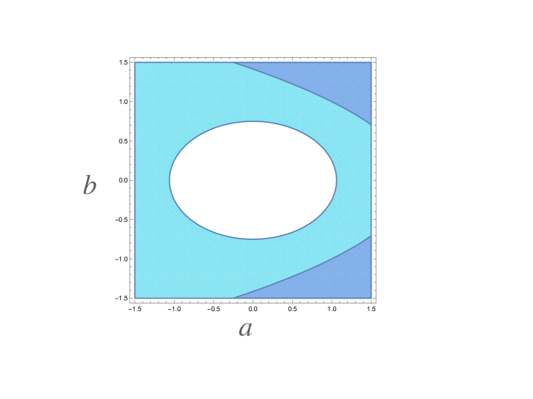
Figure 2: The region of block-positivity (outside the ellipse) overlaps with the region of negative eigenvalues for $W_{5}$, which is indicated by the colored regions in the right corners. Consequently, $W_{5}$ exhibits negative eigenvalues within this overlapping region.

5 Construction of EW for particular entangled states

In this section, our objective is to illustrate how the entanglement of an arbitrary state can be determined using the method outlined in this paper. We will elucidate the approach for creating the desired entanglement witness through two examples. The first example focuses on identifying Bell-Diagonal states, while the second pertains to a PPT entangled state.

Example 1:

The Bell-diagonal states have the following form:

$$\rho=\sum_{i,j=0,1}p_{ij}|\psi_{ij}\rangle\langle\psi_{ij}|,$$

where

$$\begin{split}&|\psi_{00}\rangle=\frac{1}{\sqrt{2}}(|00\rangle+|11\rangle),\quad|\psi_{10}\rangle=\frac{1}{\sqrt{2}}(|00\rangle-|11\rangle),\\ &|\psi_{01}\rangle=\frac{1}{\sqrt{2}}(|01\rangle+|10\rangle),\quad|\psi_{11}\rangle=\frac{1}{\sqrt{2}}(|01\rangle-|10\rangle).\end{split}$$

This state in the normalized Pauli basis is written as:

$$\rho=\frac{1}{4}(I\otimes I+2\sum_{i=1}^{3}t_{i}\Gamma_{i}\otimes\Gamma_{i}),$$ (68)

where $\Gamma_{i}=\frac{1}{\sqrt{2}}\Sigma_{i}$, and

$$\begin{split}&t_{1}=p_{00}+p_{01}-p_{10}-p_{11},\\ &t_{2}=-p_{00}+p_{01}+p_{10}-p_{11},\\ &t_{3}=p_{00}-p_{01}+p_{10}-p_{11}.\end{split}$$

We know that all separable Bell-Diagonal states lies within region $\sum_{i=1}^{3}|t_{i}|\leq 1$[23]. To identify the entanglement of this state, considering the non-zero coefficients in eq. (68), we take into account the following EW:

$$W=I\otimes I+\sum_{i=1}^{3}c_{i}\Gamma_{i}\otimes\Gamma_{i}.$$ (69)

To determine the coefficients $c_{i}$ in such a way that the introduced entanglement witness can identify the Bell-Diagonal state, we need to minimize the value of $\operatorname{Tr}(W\rho)$:

$$\operatorname{Tr}(W\rho)=1+\frac{1}{2}\sum_{i=1}^{2}c_{i}t_{i}.$$

Applying conditions (39) to the coefficients $c_{i}$ leads to:

$$c_{i}^{2}\leq 4.$$

To obtain the minimum value of $\operatorname{Tr}(W\rho)$, each of the $c_{i}t_{i}$ must take on the most possible negative value. For this purpose, we choose the coefficients $c_{i}$ as follows:

$$c_{i}=-2\textrm{ sgn}(t_{i}),$$

which leads to $c_{i}t_{i}=-2|t_{i}|$. Thus we have

$$\operatorname{Tr}(W\rho)=1-\sum_{i=1}^{3}|t_{i}|.$$

This equation will be negative if $\sum_{i=1}^{3}|t_{i}|>1$, which completely indicates the entangled Bell-Diagonal states.

Example 2:

In this example, we demonstrate that the method explained in this paper can identify PPT entangled states, and thus, it can generate indecomposable EWs. It has been shown in [24] that the following state is PPT entangled state when $x\neq 1$ (for $x=1$ this is a separable state):

$$\rho=\frac{1}{N}\left(\begin{array}[]{ccccccccc}1&0&0&0&1&0&0&0&1\\ 0&\frac{1}{x}&0&0&0&0&0&0&0\\ 0&0&x&0&0&0&0&0&0\\ 0&0&0&x&0&0&0&0&0\\ 1&0&0&0&1&0&0&0&1\\ 0&0&0&0&0&\frac{1}{x}&0&0&0\\ 0&0&0&0&0&0&\frac{1}{x}&0&0\\ 0&0&0&0&0&0&0&x&0\\ 1&0&0&0&1&0&0&0&1\\ \end{array}\right).$$

Here $N$ is the normalization factor and $x>0$. As the coefficient $N$ doesn’t impact the identification of entanglement, we can disregard it. The above state can be written in the basis of normalized Gell-Mann matrices as follows:

$$\begin{split}\rho_{x}=&\left(\frac{x}{3}+\frac{1}{3x}+\frac{1}{3}\right)I\otimes I+\Gamma_{1}\otimes\Gamma_{1}+\Gamma_{2}\otimes\Gamma_{2}+\Gamma_{3}\otimes\Gamma_{3}-\Gamma_{4}\otimes\Gamma_{4}-\Gamma_{5}\otimes\Gamma_{5}-\Gamma_{6}\otimes\Gamma_{6}\\ &+\left(-\frac{x}{2}-\frac{1}{2x}+1\right)\Gamma_{7}\otimes\Gamma_{7}+\left(\frac{\sqrt{3}}{2x}-\frac{\sqrt{3}x}{2}\right)\Gamma_{7}\otimes\Gamma_{8}\\ &+\left(\frac{\sqrt{3}x}{2}-\frac{\sqrt{3}}{2x}\right)\Gamma_{8}\otimes\Gamma_{7}+\left(-\frac{x}{2}-\frac{1}{2x}+1\right)\Gamma_{8}\otimes\Gamma_{8}.\end{split}$$ (70)

Now, we want to examine for which values of x we can identify the entanglement of this state using the method explained in the previous example. We take the EW as follows:

$$W=I\otimes I+\sum_{i=1}^{6}c_{i}\Gamma_{i}\otimes\Gamma_{i}+c_{7}\Gamma_{7}\otimes\Gamma_{8}+c_{8}\Gamma_{8}\otimes\Gamma_{7},$$

in which, according to conditions 12, we have $|c_{i}|\leq\frac{3}{2}\ \ i=1\cdots 8$ . Note that if we consider our EW as $W=I\otimes I+\sum_{i=1}^{8}c_{i}\Gamma_{i}\otimes\Gamma_{i}$, no entangled state can be detected. Similar to the reasoning provided in the previous example, the minimum value of $\operatorname{Tr}(W\rho)$ is obtained when $c_{i}r_{i}=-\frac{3}{2}|r_{i}|$, where $r_{i}$ are the coefficients of the Gell-Mann matrices in eq. (70). Hence the minimum value of $\operatorname{Tr}(W\rho)$ would be

$$\begin{split}\operatorname{Tr}(W\rho)=-6+3\left(x+\frac{1}{x}\right)-\frac{3\sqrt{3}}{{2}}\left|x-\frac{1}{x}\right|.\end{split}$$

It is clear that there can be two cases here:

• $x>1$
  Considering $\operatorname{Tr}(W\rho)<0$, the allowed values for this case is $x>1$.

• $x<1$
  Considering $\operatorname{Tr}(W\rho)<0$, the allowed values for this case is $0.154701<x<1$.

Thus, we have demonstrated that the entanglement witness constructed using the method in this paper can effectively identify the entanglement of $\rho_{x}$, a PPT entangled state, for almost all values of x except for the narrow range $0<x<0.154701$. This indicates that this approach can also produce in-decomposable EW.

6 Conclusion

In this paper, a general and practical method for constructing EWs for two particle systems with different dimensions was presented. We used two alternative methods for this construction both of which are based on the Mehta’s lemma for positive matrices. Our construction offers a straightforward and flexible approach to construct EW’s when one has limited experimental setups. In this approach, it is sufficient to select the desired measurements and then construct EW based on arbitrary coefficients for each measurement. We presented several examples each emphasizing a different aspect of our construction. In particular, it was demonstrated that the proposed method has the capability to generate indecomposable entanglement witnesses, making it a promising candidate for identifying PPT entangled states. We have only taken the first steps toward a construction of EW’s in different dimensions. Explorations of many of their properties, like optimality, extremality, exposedness [8] and their classification remain for our future investigations.

Appendix A Appendix: Proof of Equation (32)

Although equation (32) can be verified by explicit calculation for low dimensions like $d=2$ and $d=3$, it is desirable to prove it for arbitrary dimensions. An orthonormal basis of Hermitian operators for the space of $d$ dimensional matrices $M_{d}$ is given by the Gell-Mann matrices,

$$X_{kl}:=\frac{1}{\sqrt{2}}(|k,l\rangle+|l,k\rangle),\hskip 28.45274ptY_{kl}:=-\frac{i}{\sqrt{2}}(|k\rangle\langle l|-|l\rangle k|)\ \ \ \ \ \ \ \ 1\leq k<l\leq d,$$

and

$$Z_{k}:=\frac{1}{\sqrt{k(k+1)}}\Big{[}\sum_{i=1}^{k}|i\rangle\langle i|-k|k+1\rangle\langle k+1|\Big{]},\ \ \ \ I=\frac{1}{\sqrt{d}}\sum_{i=1}^{d}|i\rangle\langle i|.$$

We now note that the expression

$$A=\sum_{\alpha}E_{\alpha}\otimes E_{\alpha},$$ (71)

is invariant under the transformation of the form $E_{\alpha}\longrightarrow F_{\alpha}:=U_{\alpha\beta}E_{\beta}$, where $U$ is a unitary matrix. This puts $A_{d}$ in the form

$$A_{d}=\sum_{\alpha}F_{\alpha}\otimes F_{\alpha}^{\dagger},$$ (72)

where $F_{\alpha}$ are orthonormal, but no longer Hermitian. With such a transformation we can change the initial basis (say the Gell-Mann matrices) to the form

$$F_{k,l}=|k\rangle\langle l|,\ \ \ 1\leq i\leq j\leq d,$$ (73)

which immediately leads to the desired result, namely

$$\sum_{\alpha}F_{\alpha}\otimes F_{\alpha}^{\dagger}=\sum_{i,j}|i,j\rangle\langle j,i|=P,$$ (74)

where $P$ is the permutation operator.

References

- [1] Yue Yu. Advancements in applications of quantum entanglement. Journal of Physics: Conference Series, 2012(1):012113, sep 2021.
- [2] Nanxi Zou. Quantum entanglement and its application in quantum communication. Journal of Physics: Conference Series, 1827(1):012120, mar 2021.
- [3] Aditi Sen. Quantum entanglement and its applications. Current Science, 112:1361, 2017.
- [4] Leonid Gurvits. Classical complexity and quantum entanglement. Journal of Computer and System Sciences, 69(3):448–484, 2004. Special Issue on STOC 2003.
- [5] Reinhard F. Werner. Quantum states with einstein-podolsky-rosen correlations admitting a hidden-variable model. Phys. Rev. A, 40:4277–4281, Oct 1989.
- [6] Asher Peres. Separability criterion for density matrices. Physical Review Letters, 77(8):1413–1415, aug 1996.
- [7] Michał Horodecki, Paweł Horodecki, and Ryszard Horodecki. Separability of mixed states: necessary and sufficient conditions. Physics Letters A, 223(1-2):1–8, nov 1996.
- [8] Dariusz Chruściński and Gniewomir Sarbicki. Entanglement witnesses: construction, analysis and classification. Journal of Physics A: Mathematical and Theoretical, 47(48):483001, nov 2014.
- [9] Barbara M. Terhal. Detecting quantum entanglement. Theoretical Computer Science, 287(1):313–335, 2002. Natural Computing.
- [10] Otfried Gühne and Géza Tóth. Entanglement detection. Physics Reports, 474(1):1–75, 2009.
- [11] Joonwoo Bae, Dariusz Chruściński, and Beatrix C. Hiesmayr. Mirrored entanglement witnesses. npj Quantum Information, 6(1):15, 2020.
- [12] Bihalan Bhattacharya, Suchetana Goswami, Rounak Mundra, Nirman Ganguly, Indranil Chakrabarty, Samyadeb Bhattacharya, and A S Majumdar. Generating and detecting bound entanglement in two-qutrits using a family of indecomposable positive maps. Journal of Physics Communications, 5(6):065008, jun 2021.
- [13] M. Weilenmann, B. Dive, D. Trillo, E. A. Aguilar, and M. Navascués. Entanglement detection beyond measuring fidelities. Phys. Rev. Lett., 124:200502, May 2020.
- [14] Vahid Jannessary, Fatemeh Rezazadeh, Sadegh Raeisi, and Vahid Karimipour. Witnessing entanglement of remote particles with incomplete teleportation. Phys. Rev. A, 108:042421, Oct 2023.
- [15] Katarzyna Siudzińska and Dariusz Chruściński. Entanglement witnesses from mutually unbiased measurements. Scientific Reports, 11(1):22988, 2021.
- [16] Tao Li, Le-Min Lai, Deng-Feng Liang, Shao-Ming Fei, and Zhi-Xi Wang. Entanglement witnesses based on symmetric informationally complete measurements. International Journal of Theoretical Physics, 59(11):3549–3557, oct 2020.
- [17] Kun Wang and Zhu-Jun Zheng. Constructing entanglement witnesses from two mutually unbiased bases. International Journal of Theoretical Physics, 60(1):274–283, 2021.
- [18] Dariusz Chruściński and Andrzej Kossakowski. Spectral conditions for positive maps and entanglement witnesses. Journal of Physics: Conference Series, 284(1):012017, mar 2011.
- [19] Dariusz Chruściński, Gniewomir Sarbicki, and Filip Wudarski. Entanglement witnesses from mutually unbiased bases. Physical Review A, 97(3), mar 2018.
- [20] Anindita Bera, Gniewomir Sarbicki, and Dariusz Chruściński. A class of optimal positive maps in m. Linear Algebra and its Applications, 668:131–148, jul 2023.
- [21] M.L. Mehta. Matrix Theory: Selected Topics and Useful Results. Hindustan Publishing Corporation, 1989.
- [22] Reinhold A Bertlmann and Philipp Krammer. Bloch vectors for qudits. Journal of Physics A: Mathematical and Theoretical, 41(23):235303, may 2008.
- [23] Elias Riedel Gårding, Nicolas Schwaller, Chun Lam Chan, Su Yeon Chang, Samuel Bosch, Frederic Gessler, Willy Robert Laborde, Javier Naya Hernandez, Xinyu Si, Marc-André Dupertuis, et al. Bell diagonal and werner state generation: Entanglement, non-locality, steering and discord on the ibm quantum computer. Entropy, 23(7):797, 2021.
- [24] Joonwoo Bae, Anindita Bera, Dariusz Chruś ciński, Beatrix C Hiesmayr, and Daniel McNulty. How many mutually unbiased bases are needed to detect bound entangled states? Journal of Physics A: Mathematical and Theoretical, 55(50):505303, dec 2022.