Metal Abundances of Intermediate-Redshift AGN: Evidence for a Population of Lower-Metallicty Seyfert 2 Galaxies at z = 0.3 – 0.4

Abstract

We derive oxygen abundances for two samples of Seyfert 2 (Sy2) active galactic nuclei (AGN) selected from the KPNO International Spectroscopic Survey (KISS). The two samples from KISS include 17 intermediate-redshift (0.29 $\leq$ z $\leq$ 0.42) Sy2s detected via their [O III] lines, and 35 low-redshift (z $\leq$ 0.1), H$\alpha$-detected Sy2s. The primary goal of this work is to explore whether the metallicity distribution of these two samples changes with redshift. To determine the oxygen abundances of the KISS galaxies, we use Cloudy to create a large number of photoionization model grids by varying the temperature of the accretion disk, the ratio of X-ray to UV continuum light, the ionization parameter, the hydrogen density, and the metallicity of the narrow-line region clouds. We link the results of these models to the observed [O III]/H$\beta$ and [N II]/H$\alpha$ emission-line ratios of the KISS sample on the BPT diagram, interpolating across the model grids to derive metallicity. The two redshift samples overlap substantially in terms of derived metal abundances, but we find that some of the intermediate-redshift Sy2 galaxies possess lower abundances than their local universe counterparts. Our analysis provides evidence for modest levels of chemical evolution ($0.18\pm 0.06$ dex) over $3-4$ Gyrs of look-back time. We compare our results to other AGN abundance derivation methods from the literature.

1 Introduction

Active galactic nuclei (AGN) are the most luminous, persistent sources of light in the universe, often outshining all the stars in their host galaxies. The strong emission lines presented in AGN spectra can be used to estimate chemical abundances at a wide range of redshifts. Therefore, in order to study how the universe chemically evolves over time, it is to study the evolution of AGN abundances with redshift.

However, AGN abundance determination methods have received little attention when compared to their star-forming galaxy (SFG) counterparts. There is a general consensus for SFGs that the determination of the electron temperature allows for the derivation of the metallicity Z (Kennicutt et al., 2003; Hägele et al., 2008; Yates et al., 2012; Pérez-Montero, 2017; Maiolino & Mannucci, 2019). This method is called the $T_{e}$-method.

There are two problems with the $T_{e}$-method when it comes to determining AGN abundances. times weaker than [O III]$\lambda 5007$ at the characteristic abundances of AGN, it is not easily detected. the $T_{e}$-method is only applicable to objects with high-excitation lines or low metallicity, a problem of the method for both SFG and AGN abundance determinations (van Zee et al. 1998; Castellanos et al. 2002; Díaz et al. 2007; Pilyugin 2007; Sanders et al. 2016, among others).

Second, when the line is detected in AGN, the resulting electron temperature is often higher than expected and the abundances estimated from it are unrealistically low (Dors et al., 2015, 2020b). The reasons for this are not well understood. Some authors suggest shocks enhance the [O III]$\lambda 4363$ linehough the signatures of strong shocks are not found in Seyfert 2 spectra (e.g., Zhang et al. 2013; Dors et al. 2015). Komossa & Schulz (1997) built photoionization models of nuclei and considered inhomogeneities in the electron density to attempt to reproduce the narrow optical emission lines observed in these galaxies. They successfully reproduced the [S III]$\lambda\lambda 9069,9531$ emission lines, and lines like [Fe III]$\lambda 4658$ and [Fe VII]$\lambda 6087$, but failed to reproduce the [O III]$\lambda 4363/\lambda 5007$ line ratio.

Dors et al. (2020a) the discrepancy between the $T_{e}$-method and other methods. They found that the relationship derived for H II regions between temperatures of the low ($t_{2}$) and high ($t_{3}$) ionization gas does not apply to determining AGN abundances. They derived a new expression for the $t_{2}-t_{3}$ relation for nuclei and reduced the average discrepancy between the $T_{e}$-method and other abundance methods by 0.4 dex. However, a systematic difference is still present when compared to other methods.

To combat these issues, additional relationships between Z and stronger emission-line ratios have been suggested. These methods are called strong-line methods. For a review see Kewley et al. 2019. Currently there are only a handful of relationships that tie optical emission-line ratios to AGN abundance. The first relationship between metallicity and optical emission-line ratios was developed by Storchi-Bergmann et al. (1998). Since then other relationships have been suggested (see Castro et al. 2017; Carvalho et al. 2020; Flury & Moran 2020; Dors 2021) but none agree perfectly with each other (Dors et al., 2020b). Thus, if one wishes to determine the abundance of a sample of AGN with optical emission-line data, the way forward is not always clear.

In this work, we seek to derive oxygen abundances for two distinct samples of AGN, one at low redshifts (z $\leq$ 0.1) and the other at . Both samples of Sy2s are derived from the KPNO International Spectroscopic Survey (KISS) (Salzer et al., 2000). The primary goal of this project is to determine if the metallicity distribution of these two samples changes with redshift.

To determine the oxygen abundances of the KISS sample of galaxies, we use Cloudy (Ferland et al., 2017) to create a set of 3240 photoionization models by varying the accretion disk temperature, ratio of X-ray to UV continuum light, ionization parameter, hydrogen density, and metallicity of the narrow-line region clouds. We link the results of these models to the observed [O III]/H$\beta$ and [N II]/H$\alpha$ emission-line ratios of the KISS sample on the Baldwin, Philips, Terlevich (BPT; Baldwin et al. 1981) diagram, interpolating across the model grids to derive metallicity.

Section 2 details the properties of the observational data from the KISS survey. Next, Section 3 illustrates how the photoionization models are created and how the final metallicities are derived for the Sy2 sample. Section 4 presents the results of using these models to derive the abundances. Finally, Section 5 discusses these results, plots a mass-metallicity relationship, and compares this work to some of the other methods of determining AGN abundances from the literature.

2 Observational Data

Our sample comes from the KPNO International Spectroscopic Survey (KISS; Salzer et al. 2000). KISS is an objective-prism survey with optical data acquired using the Burrell Schmidt telescope. It was the first purely digital objective-prism survey designed to find nearby emission-line galaxies (ELGs) using wide-field spectroscopy and its goal was to provide a comprehensive survey of ELGs in the nearby universe. The survey contains a statistically complete, emission-line-flux-limited sample of and and has a limiting line flux of about $1.0\times 10^{-15}$ erg s^-1 cm^-2.

KISS’s objective-prism spectra covered two wavelength ranges. The first, known as KISS red (KISSR), covered $6400-7200$ Å and detects objects primarily by their H$\alpha$ line (Salzer et al., 2001; Gronwall et al., 2004b; Jangren et al., 2005a). The second, known as KISS blue (KISSB), covered $4800-5500$ Å and detects objects primarily by their [O III]$\lambda$5007 line (Salzer et al., 2002). We limit our analysis to the KISSR sample for this work because it represents sample of galaxies . Furthermore, the sky overlap of the KISSB survey with the first KISSR catalog (Salzer et al., 2001) results in most of the KISSB objects being included in KISSR.

While the original objective-prism spectra were enough to determine the presence of emission lines in the KISS galaxies, follow-up spectroscopy was carried out to determine accurate redshifts and the activity class of each galaxy in the KISS sample. See Hirschauer et al. (2018) for a more recent summary of the full spectroscopic follow-up of KISS.

Each galaxy in the KISSR sample also has stellar mass estimates determined using spectral energy distribution (SED) fitting as described in Hirschauer et al. (2018). These measurements can be utilized to derive a stellar-mass-metallicity relationships which will be useful for further analysis later in this work.

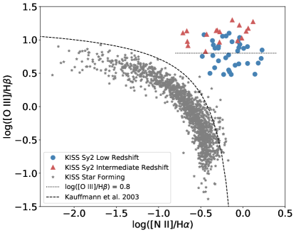
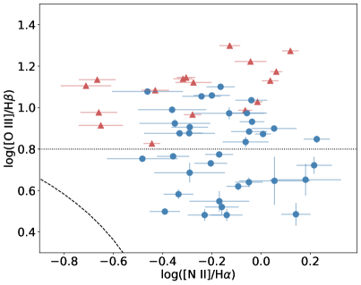
Figure 1: We present two emission-line ratio diagnostic diagrams, known as BPT diagrams (Baldwin et al., 1981). Top: We present the star-forming and Seyfert 2 AGN from the KISSR sample. LINERs have been excluded. The Seyfert 2 galaxies are split into two samples based on redshift and are plotted as red triangles and blue circles respectively. The star-forming galaxies plotted as gray stars. The Kauffmann et al. (2003) line, which separates the star-forming and AGN regions of the plot, is shown as a dashed line. Finally, the horizontal dotted line at log([O III]/H$\beta$) = 0.8 denotes the selection limit for the intermediate-redshift Seyfert 2s, as described in the text. Bottom: The Seyfert 2 region of the BPT diagram is shown in more detail. he Kauffmann et al. (2003) and log([O III]/H$\beta$) = 0.8 lines.

The KISSR star-forming and Sy2 sample are displayed on a diagram in the top panel of Figure 1. The empirical Kauffmann et al. (2003) line, which separates the star-forming and AGN regions of the plot, is shown as a dashed line. Spectral classification (SFG or AGN) for the KISS sample are determined by visual inspection of . Generally, an object is classified as a Sy2 AGN if it falls above the empirical Kauffmann et al. (2003) demarcation line and has a log([O III]/H$\beta$) emission-line ratio greater than 0.5. Objects with log([O III]/H$\beta$) less than 0.5, while still lying above the Kauffmann et al. (2003), line are generally considered to be a low-ionization nuclear emission region (LINER; Heckman 1980), as is consistent with traditional classification schemes (Ho et al., 1997). LINERs are excluded from the plot for clarity.

The emission-line ratios displayed in the figure have been corrected for reddening and underlying Balmer absorption. In the case of the underlying absorption, we apply a 2 Å correction which is consistent with Skillman & Kennicutt (1993) and Hirschauer et al. (2022).

In total, the KISSR sample contains 1455 star-forming galaxies and 52 Sy2 AGN . A majority of these objects are detected via their H$\alpha$ emission lines at z $\leq$ 0.1. However, in $\thicksim$2% of cases, objects were detected by their [O III]$\lambda$5007 emission lines that had been redshifted into the KISSR filter’s wavelength range (Salzer et al., 2009). Many of these [O III]-detected objects are AGN and had redshifts between 0.29 and 0.42. Therefore, this work, which attempts to derive abundances for the KISS AGN, uses two distinct samples of galaxies from KISS. These samples probe different redshift windows. The first sample includes 17 [O III]-detected (0.29 $\leq$ z $\leq$ 0.42), intermediate-redshift Sy2 AGN. The second contains 35 H$\alpha$-detected (z $\leq$ 0.1), low-redshift Sy2 AGN. These are plotted in Figure 1 as red triangles and blue circles respectively. The star-forming galaxies are represented by gray stars.

It is important to note that, because the KISS sample is emission-line flux limited, it is only able to detect the strongest-lined systems via the [O III] line in the intermediate-redshift galaxies. This $\log$[O III]$\lambda$5007/H$\beta$ $\approx$ 0.8. This limit is marked on the plot as a dotted line. We stress that this limit is strictly caused by the sensitivity limits of the survey. It is not a limit set by the physical characteristics of the galaxies themselves.

We focus in on the Sy2 sample in the bottom panel of Figure 1. . There appears to be an excess of intermediate-redshift galaxies with low [N II]$\lambda$6584 to H$\alpha$ ratios compared to the lower-redshift sample.

3 Methodology

We use version 17.01 of Cloudy (Ferland et al., 2017) to create grids of AGN photoionization models that span the entire area of the KISSR sample on the BPT diagram. A metallicity is then assigned to each galaxy based on its location inside the grids. Section 3.1 discusses the parameters specified to construct the models, Section 3.2 presents the final model grids, and Section 3.3 outlines how a final metallicity value was assigned to each galaxy.

3.1 Photoionization Model Parameters

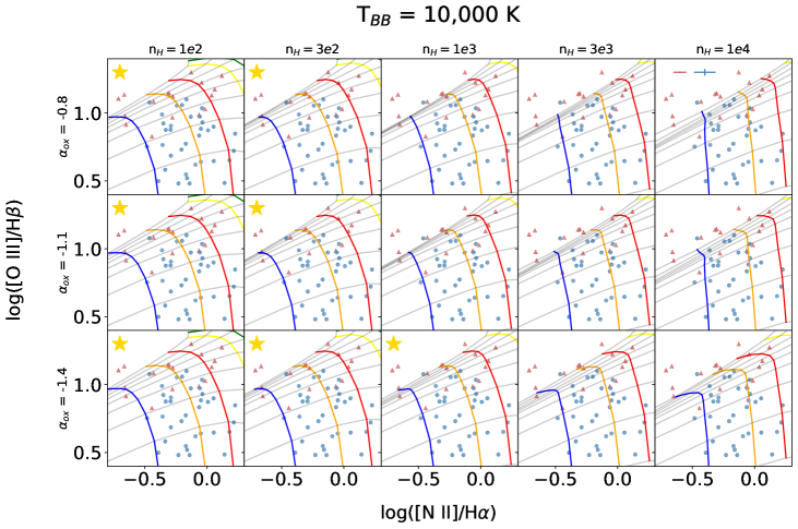
Figure 2: We present the photoionization model grids created as part of this project overlaid on the BPT diagram of the KISSR sample. This set of 15 grids is for models calculated with $T_{BB}=10^{4}$ K. Going from left to right is increasing hydrogen density and from top to bottom is decreasing $\alpha_{ox}$ values. The KISS Sy2 intermediate-redshift AGN are shown as red triangles and the low-redshift AGN are shown as blue circles as before. Each square of the group of 15 has a set of models grids represented by colored lines. Models are calculated with 2 (green), 1.5 (yellow), 1 (red), 0.75 (orange), 0.5 (blue), and 0.25 (not shown) solar metallicity. The gray lines are different ionization parameters with more negative ($-3.5$) starting to the lower right and increasing to less negative ($-1.5$) toward the upper left. odels that overlay 85% of the KISSR sample are kept to use in the final metallicity calculation. They are marked with a gold star in the upper left of the square.

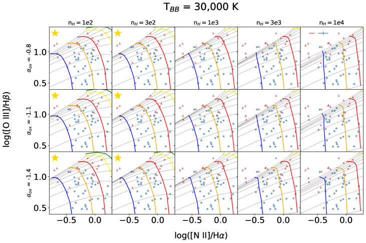
Figure 3: Similar to Figure 2. This set of 15 is for grids of models calculated with $T_{BB}=3\times 10^{4}$ K.

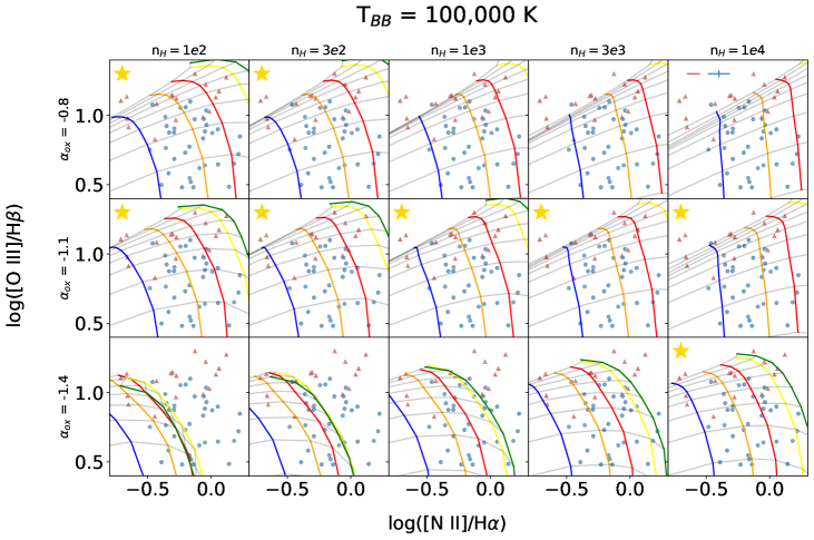
Figure 4: Similar to Figure 2. This set of 15 is for grids of models calculated with $T_{BB}=10^{5}$ K.

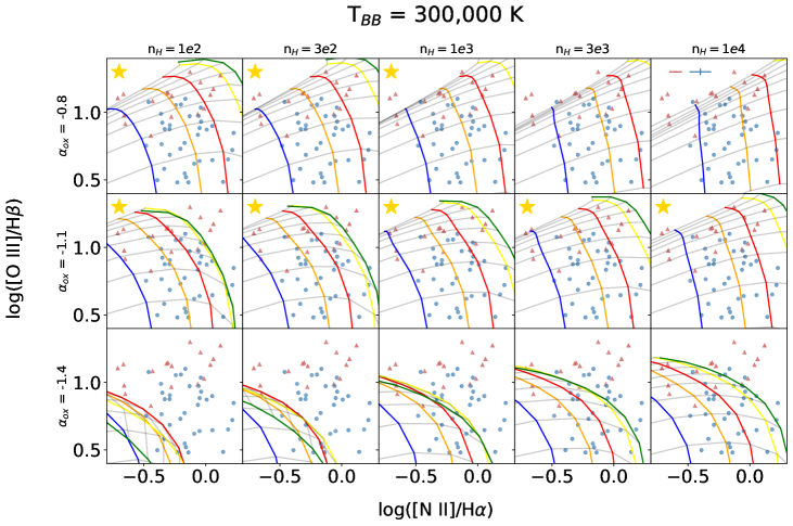
Figure 5: Similar to Figure 2. This set of 15 is for grids of models calculated with $T_{BB}=3\times 10^{5}$ K.

To create accurate approximations for the NLRs of the KISSR Sy2 sample, four main parameters had to be defined: the shape of the spectral energy distribution (SED), the ionization parameter (U), the hydrogen density (n_H), and the metallicity (Z).

(i) SED: To specify the shape of the radiation field, we use Cloudy’s AGN command produces a power law with two components the following form:

$$f_{\nu}=\nu^{\alpha_{uv}}\exp\left(\frac{-h\nu}{kT_{BB}}\right)\exp\left(\frac{-kT_{IR}}{h\nu}\right)+a\nu^{\alpha_{x}}$$ (1)

The first component represents the “Big Bump” (BB, sometimes referred to as “Big Blue Bump”) which peaks at 1 Ryd. The BB is thought to be a result of thermal emission from the accretion disk. ue to the accretion disk’s temperature varying with from the black hole, a combination of many black bodies with different temperatures .

In this work we keep $\alpha_{uv}$, which represents the low-energy slope of the BB, at its default value of $-0.5$. However, we allow the value of the BB temperature ($T_{BB}$) to vary, assigning values of $10^{4}$, $3\times 10^{4}$, $10^{5}$, and $3\times 10^{5}$ K. his range of model input values was chosen in order to cover the parameter space exhibited by the KISS emission-line ratios. Without the higher $T_{BB}$ models, two of the KISSR intermediate-redshift AGN are not covered by any of these model grids.

The second component is a power law with spectral index $\alpha_{x}$t represents the non-thermal X-ray radiation is kept at its default value of $-1$. The X-ray to UV flux ratio, represented by $\alpha_{ox}$, is used to specify the coefficient $a$ and describes the continuum between 2 keV and 2500 Å. In this work we vary $\alpha_{ox}$ between $-0.8$, $-1.1$, and $-1.4$. This used in Carvalho et al. (2020) and covers the range ypically specified for AGN (Ho, 1999; Miller et al., 2011; Zhu et al., 2019).

(ii) Ionization Parameter: The ionization parameter (U) has the functional form

$$\text{U}=\frac{\text{Q(H)}}{4\pi r^{2}_{0}n_{H}c}$$ (2)

and is the ratio of hydrogen-ionizing photons to total-hydrogen density. Q(H) [s^-1] is the number of ionizing photons emitted by the source , $r_{0}$ [cm] is the distance between the center of the source and the cloud, $n_{H}$ [cm^-3] is the hydrogen density, and $c$ is the speed of light.

For this work, we vary the logarithm of the ionization parameter from $-3.5\leq\log\text{U}\leq-1.5$ in 0.25 dex steps. This is similar to the range used in Castro et al. (2017), Dors et al. (2019), and Carvalho et al. (2020) for AGN.

(iii) The Hydrogen Density: The hydrogen density was varied between models to be $n_{H}=100,\ 300,\ 1000,\ 3000,$ and $10,000$ cm^-3. Generally, the range of densities in the NLRs of AGN cover the 100 to 3000 cm^-3 range (Vaona et al., 2012; Zhang et al., 2013; Dors et al., 2014; Flury & Moran, 2020) but can extend to higher densities (Revalski et al., 2018). This range of parameters allows us to probe the entire range of the sample while staying under the critical densities for the emission lines used in this study.

Cloudy

(iv) Metallicity: We allow the metallicity in the models to vary, setting it to the following values: $\text{Z}/\text{Z}_{\odot}$ = 0.25, 0.5, 0.75, 1, 1.5, and 2. solar abundance of $\log(\text{O/H})+12=8.69$. Models assuming $\text{Z}/\text{Z}_{\odot}>2$ produce similar emission-line ratios to models with metallicity less than 2 so, in order to avoid in the model , the range was limited to $\text{Z}/\text{Z}_{\odot}\leq 2$. These values for our models are similar to previous works and have been found in AGN at a wide range of redshifts (see Carvalho et al. (2020) and the references therein).

The abundances of all elements are scaled linearly with metallicity (O/H) except nitrogen and helium. Nitrogen was scaled with the following equation from Carvalho et al. (2020) based on work from Dors et al. (2017):

$$\log(\text{N/O})=1.29\times(12+\log(\text{O/H}))-11.84$$ (3)

is valid for $\text{Z}/\text{Z}_{\odot}\gtrsim 0.2$ and was derived using a sample of Seyfert 2 AGN at $z<0.1$ and a sample of H II regions.

It is necessary to introduce scaling relation because nitrogen has two separate methods of production. For stars in low metallicity galaxies, if the oxygen and carbon are produced in the star by helium burning, then the amount of nitrogen produced is independent of the initial heavy element abundance and the nitrogen has a primary origin . For stars in high metallicity galaxies, the amount of nitrogen produced is proportional to the initial heavy-element abundance. It is produced from the burn of these heavy elements and is said to have a secondary origin . The relation is assumed in order to take into account the secondary nitrogen origin.

For the helium abundance, a scaling relation is necessary. Helium has a high initial abundance as a result of the Big Bang so helium only scales weakly with metallicity. For the Helium abundance we follow a relation found in Dopita et al. (2006).

$$\frac{\text{He}}{\text{H}}=0.0737+0.024\times\text{Z}/\text{Z}_{\odot}$$ (4)

3.2 Presentation of Model Grids

The output of the models can be seen overlaid on the KISSR sample in Figures 2 through 5. In total we have constructed 60 different sets of grids over a wide range of AGN parameters that cover the parameter space of the KISSR sample. Each set of grids is divided by $T_{BB}$ into groups of 15. Inside each of the groups, the hydrogen density, $n_{H}$, increases from left to right and the X-ray to UV flux ratio, $\alpha_{ox}$, decreases from top to bottom. The KISS Sy2 intermediate-redshift AGN are shown as red triangles and the low-redshift AGN are shown as blue circles. Each square in the group of 15 has a set of models grids represented by colored lines. These lines span the metallicity range of $\text{Z}/\text{Z}_{\odot}=0.25-2$. The gray lines show the changing ionization parameter, U, with more negative ($-3.5$) starting to the lower right and increasing to less negative ($-1.5$) to the upper left. .

Each of the four $T_{BB}$ groups contains 15 grids, each grid contains six metallicity values and nine ionization parameter values. In total 3240 models were created as part of this work in order to cover the full range of relevant parameter space.

3.3 Model Selection and Calculating Metallicity

Since these models explore such a wide range of parameter space, some of the model grids do a better job of the KISSR sample than others. to only use model grids that 85% of the total KISSR Sy2 sample. After we implemented this requirement, a total of 29 grids remained. These are marked with a gold star in Figures 2 through 5.

Once the grids are identified, a metallicity must be calculated for each object. For each of the 29 model grids, each galaxy is located within a box-shaped region of the grid bounded by two values of the metallicity and two values of the ionization parameter. The galaxy’s position is used to interpolate between the edges of the box to assign each galaxy a metallicity and ionization parameter. If a point is outside the grid’s area, it is not assigned a value for that set of models.

After this process is done, each KISS AGN now has a number of different interpolated values for Z and U depending on where that galaxy falls in the various grids. To get the final value of Z for each AGN we take the ($\sigma$) of the measurements. We remove from the list of estimated metallicities anything that is more than 3$\sigma$ from the median, recalculate the median and standard deviation, and iterate an additional time. the mean for each galaxy and set th as its final value for Z. A similar process is done to calculate a theoretical U value for each KISSR AGN which we use later in Section 4 to conduct further analysis on the KISSR sample.

$$\log(\text{O}/\text{H})+12=\log(\text{Z}/\text{Z}_{\odot}\times 10^{-3.31})+12$$ (5)

where the solar oxygen abundance is log(O/H) = $-3.31$ (Asplund et al., 2009).

4 Results

e plot the KISS Sy2 sample on a BPT diagram in Figure 6. the galaxies are assigned colors based on the metallicity derived from the photoionization models. We construct a histogram of the derived abundances and plot the intermediate- and low-redshift samples separately in Figure 7.

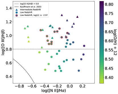
Figure 6: BPT diagram of the KISS Sy2 sample by their derived log(O/H) + 12 values. The intermediate-redshift sample are triangles and the low-redshift sample are circles. The Kauffmann et al. (2003) line is shown as a dashed line in the lower left. The horizontal dotted line at log([O III]/H$\beta$) = 0.8 denotes the selection limit for the intermediate-redshift Seyfert 2s, as described in the text. The low-redshift sample has been split into shown in Figures 8 and 9. If the low-redshift galaxy is above the log([O III]/H$\beta$) = 0.8 line, it is included in Figure 8. For a low-redshift galaxy to be included in Figure 9, it must have a derived ionization parameter, U, that is greater than the minimum ionization parameter derived for the intermediate-redshift sample. These sources are outlined in red.

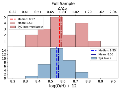
Figure 7: The full sample of KISS AGN are displayed in a histogram with the intermediate-redshift AGN in red in the top panel and low-redshift AGN in blue on the bottom panel. log(O/H) + 12 is shown on the bottom x axis and $\text{Z}/\text{Z}_{\odot}$ is shown on the top x axis. Number is on the y axis. Median and mean values of the two samples are shown as a dashed and dashed-dotted line.

here is essentially no difference between the mean metallicity of the intermediate- and low-redshift AGN . However, there is a difference in the distribution of the metallicity values. large percentage of the low-redshift sample is concentrated in the 8.4 to 8.7 log(O/H) + 12 range whereas the intermediate-redshift sample is more evenly distributed across the metallicity bins.

t is not entirely to compare the entirety of these two samples together. The H$\alpha$-detected sample finds all the AGN in the volume of the survey. However, because the KISS sample is emission-line flux limited, the sensitivity of the survey limits the detection of the [O III]-selected intermediate-redshift sample to the strongest-lined systems. That is, it detects the AGN with high [O III]/H$\beta$ ratios and high ionization parameter values.

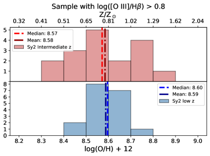
Figure 8: Similar to Figure 7, where only the low-redshift galaxies with log([O III]/H$\beta$) $>$ 0.8 are included. These objects are above the horizontal dotted line in Figure 6. The [O III]-selected, intermediate-redshift KISS Seyferts show an excess of both high- and low-metallicity objects.

In order to provide a fair comparison, we can two different but complementary the low-redshift sample. First, we limit the galaxies in the low-redshift sample according to their [O III]/H$\beta$ ratios. The intermediate-redshift sample does not extend below log([O III]/H$\beta$) of about 0.8 so as the limit for the low-redshift sample. The result is shown in Figure 8. The low-redshift points used in this comparison are above the dotted line in Figure 6.

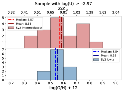
Figure 9: Similar to Figure 7, where the only low-redshift galaxies included have a derived ionization parameter, U, greater than the minimum ionization parameter calculated for the intermediate-redshift sample. These objects are outlined in red in Figure 6.

we can with similar ionization parameters. The lowest derived value of U in the intermediate-redshift sample is log(U) $=-2.97$. The result of limiting the low-redshift sample according to the ionization parameter values is shown in Figure 9 and produces similar results to Figure 8. The low-redshift points used in this comparison are outlined in red in Figure 6.

Once these effects are taken into account, we see differences in the distribution of metallicities between the two samples of galaxies, regardless of the correction method used. We highlight the following primary results.

First, the means and medians of the two samples remain comparable and there is substantial overlap in the distribution between the two samples at intermediate abundances. However, the distribution of the intermediate-redshift AGN is much broader than that of the low-redshift AGN.

Second, the intermediate-redshift sample has a higher fraction of high-metallicity AGN. The intermediate-redshift Sy2s likely include several higher mass and, therefore, higher-metallicity systems . We will explore this in further detail in Section 5.2.

Third, the intermediate-redshift sample also has a higher fraction of low metallicity AGN. This implies that there is a population of Sy2s that have lower chemical compositions at this look-back time.

To test if the two distributions are different, we performed a Kolmogorov–Smirnov test the two different redshift samples. For the full sample, there was a 47% chance that the two samples were drawn from the same population . This percentage decreased to 37% for the [O III]/H$\beta$-limited sample and 27% for the log(U)-limited sample. The results from the K-S test support the idea that there is a difference between these two samples but that the statistical significance of that difference is only modest.

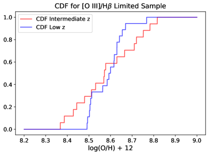
Figure 10: The cumulative distribution function associated with the intermediate-redshift sample and the subset of the low-redshift sample presented in Figure 8.

5 Discussion

5.1 The Existence of a Lower-Metallicity Seyfert 2 Sample at Intermediate Redshifts

Having identified a small population of in our intermediate-redshift sample, we now speculate about the possible reasons for the existence of this population. It is important to note that we only see the metallicity difference in a subset of the intermediate-redshift AGN and the level of metallicity difference is $0.1-0.2$ dex.

One possible explanation for why some AGN in the intermediate-redshift sample have lower abundances is related to infalling gas from the intergalactic medium. According to cosmological models, intergalactic gas was more prevalent at higher redshifts than today (e.g., Somerville & Davé 2015). If these galaxies had access to more unprocessed material, that material may flow into the centers of these galaxies. Therefore, compared to the local universe where more of the nuclear infall is from the interstellar medium of the host galaxy, the intermediate-redshift galaxies would have their metallicity content diluted. This dilution from unprocessed intergalactic gas might be what lowers the total metallicity and causes the differences between the two samples.

Another reason that might explain why the intermediate-redshift sample has lower abundances is that chemical evolution in these galaxies has had less time to progress. Ly et al. (2016) compare the mass-metallicity relation for star-forming galaxies across three redshift bins, z $<0.3$, $0.3<$ z $<0.5$, and $0.5<$ z $<1.0$, to the mass-metallicity relation found by Andrews & Martini (2013) for z $\sim 0.1$. They find, at a given stellar mass, an average offset of 0.13 dex at z $<0.3$, $-0.17$ dex at $0.3<$ z $<0.5$, and $-0.24$ dex at $0.5<$ z $<1.0$. Thus, the mass-metallicity relation shifts toward lower metallicity at fixed stellar mass with increasing look-back time. This suggests it is possible that the higher-redshift sample has lower abundances simply because they have undergone less chemical evolution.

5.2 Mass–Metallicity Relationship

It is also possible that the intermediate-redshift sample includes low metallicity galaxies because these galaxies are low mass systems and lower-mass systems tend to have lower abundances (e.g., Lequeux et al. 1979, Hirschauer et al. 2018). To test this , we can plot the metallicity against the mass using the stellar mass data presented in Hirschauer et al. (2018). Simultaneously, we can test the hypothesis that the reason for the high fraction of high-metallicity AGN in the intermediate-redshift sample is because they are higher mass and hence higher metallicity.

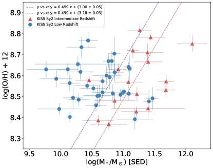
Figure 11: We plot the derived log(O/H) + 12 values for the Sy2 samples against the stellar mass of each galaxy. The KISS Sy2 intermediate-redshift AGN are shown as red triangles and the low-redshift AGN are shown as blue circles as before.

Figure 11 shows the derived log(O/H) + 12 values for the KISSR sample from this work plotted against the log of the stellar mass of each galaxy in a mass-metallicity (M–Z) plot. For completeness, the full low-redshift sample is displayed in the figure. The mass distribution for the low-redshift sample doesn’t change significantly when we apply the [O III]/H$\beta$ or log(U) limits.

he value for the intermediate-redshift sample is $\log(\text{M}_{*}/\text{M}_{\odot})=11.21\pm 0.10$ while the value for the low-redshift sample is $\log(\text{M}_{*}/\text{M}_{\odot})=10.63\pm 0.07$. Of the intermediate-redshift AGN, only two fall below the of the low-redshift sample. Thus, we can say with some certainty that the low-abundance galaxies in the intermediate-redshift sample are not lower-abundance systems because of their masses.

Additionally, from Figure 11 we can see the higher abundance intermediate-redshift AGN are also generally higher-mass systems. This lends credence to our hypothesis that the high fraction of high-metallicity AGN in the intermediate-redshift sample is likely due to them being higher mass. The KISS survey detects these galaxies at these higher redshifts because

5.3 Comparison to Previous Work

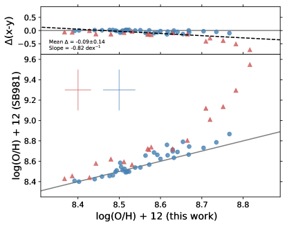
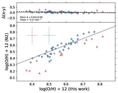
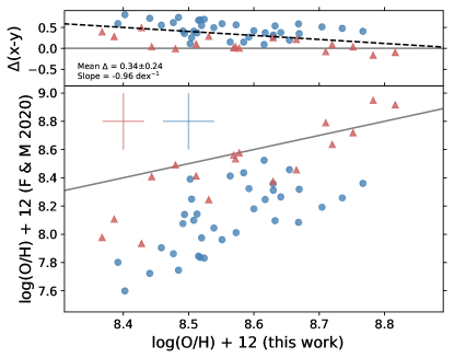
Figure 12: We plot the abundance derivations from this work against abundances derived from three different emission-line abundance methods from the literature in the bottom section of each panel. The KISS Sy2 intermediate-redshift AGN are shown as red triangles and the low-redshift AGN are shown as blue circles as before. The gray solid line is the one-to-one line . The top section of each panel is the difference between our results and the literature method’s results ($\Delta(x-y)=\text{Our Results}-\text{Literature Results}$). The gray line in this section is a result of no difference. A line with the functional form $y=m\times x+b$ is fit to the differences and is displayed as a black dashed line. The average difference and the slope of the fit line is also listed in each panel. Left: The SB98,1 method. Right: N2 method. Lower: Flury & Moran (2020) method.

There are several strong-line methods from the literature that map emission-line ratios for Sy2 AGN to abundances. We can compare the results from our work to these other methods to see if they agree. Many of the relationships developed by these authors are also based on photoionization models built with Cloudy.

The first relationship between metallicity and optical emission-line ratios was developed by Storchi-Bergmann et al. (1998). They presented two different schemes which we label SB98,1 and SB98,2. The first requires [N II]$\lambda\lambda 6548,6584$/H$\alpha$ and [O III]$\lambda\lambda 4959,5007$/H$\beta$ line ratios and the second requires [O II]$\lambda\lambda 3726,3729$/[O III]$\lambda\lambda 4959,5007$ and [N II]$\lambda\lambda 6548,6584$/H$\alpha$ line ratios. Castro et al. (2017) created the N2O2 method which is dependent on the log([N II]$\lambda 6584$/[O II]$\lambda 3727$) ratio. Carvalho et al. (2020) created the N2 method which is only dependent on the [N II]$\lambda 6584$/H$\alpha$ line ratio. Flury & Moran (2020) have developed a method for estimating abundances using the $T_{e}$-method. Their relationship uses the [O III]$\lambda 5007$/H$\beta$ and [N II]$\lambda 6584$/H$\alpha$ line ratios. Finally, Dors (2021) created a bi-dimensional relationship using $R_{23}$ and takes advantage of the [O II]$\lambda\lambda 3726,3729$, [O III]$\lambda\lambda 4959,5007$, and H$\beta$ lines. There are also several other approaches that make use of Bayesian statistics in the literature (Pérez-Montero, 2014; Thomas et al., 2018; Mignoli et al., 2019; Pérez-Montero et al., 2019).

In Dors et al. (2020b), some of these methods were compared against each other. They found that the oxygen abundance estimates from some of the strong-line methods differed from each other by up to about $0.8$ dex with the largest differences occurring when log(O/H) + 12 $\leq$ 8.5. However, the two Storchi-Bergmann et al. (1998) methods generally agree with an average difference of $-0.08$ dex.

For this work, some of the KISSR sample does not include the [O II] doublet line information. Therefore, we will focus this comparison on the methods that only use the [O III], [N II], H$\alpha$, and H$\beta$ lines. Since SB98,2 relies on [O II], and because it agrees well with SB98,1, we will only consider SB98,1 going forward. We will also consider the N2 method and the Flury & Moran (2020) method in this comparison.

The SB98,1 relationship is given by the following equation from Storchi-Bergmann et al. (1998).

$$z_{\text{SB}98,1}=8.34+0.212x-0.012x^{2}-0.002y$$ (6)

$$+0.007xy-0.002x^{2}y+6.52\times 10^{-4}y^{2}$$

$$+2.27\times 10^{-4}xy^{2}+8.87\times 10^{-5}x^{2}y^{2}$$

Here $z=\log(\text{O}/\text{H})+12$, x = [N II]$\lambda\lambda 6548,6584$/H$\alpha$  and y = [O III]$\lambda\lambda 4959,5007$/H$\beta$. It is valid for $8.4\leq\log(\text{O}/\text{H})+12\leq 9.4$ and must be corrected for electron density effects such that

$$z_{\text{final}}=z_{\text{SB}98,1}-0.1\times\log(N_{e}/300\text{ (cm}^{-1}))$$ (7)

To determine $N_{e}$ for each galaxy, we average the $n_{H}$ values from each model used to calculate the metallicity estimate for that galaxy. .

The N2 method provided by Carvalho et al. (2020) define their relationship as

$$(\text{Z}/\text{Z}_{\odot})=a^{N2}+b$$ (8)

where N2 = log([N II]$\lambda 6584$/H$\alpha$), a = 4.01 $\pm$ 0.08, and b = -0.07 $\pm$ 0.01. It is valid for $0.3\leq\text{Z}/\text{Z}_{\odot}\leq 2.0$ and z $\lesssim 0.4$.

Finally, Flury & Moran (2020) define their relationship as

$$z=7.863+1.170x+0.027y-0.369x^{2}$$ (9)

$$+0.208y^{2}-0.406xy-0.100x^{3}$$

$$+0.323y^{3}+0.354x^{2}y-0.333xy^{2}$$

where $z=\log(\text{O}/\text{H})+12$, $x$ = log([N II]$\lambda 6584$/H$\alpha$), and $y$ = log([O III]$\lambda 5007$/H$\beta$). It is valid for $7.5\leq\log(\text{O}/\text{H})+12\leq 9.0$.

Figure 12 shows the results from the comparison of these three methods plotted against our derived abundances as well as the difference, $\Delta(x-y)$, for each method. The top left panel plots the SB98,1 method against our results. The SB98,1 method does a good job matching our results at lower abundances but, as $\log(\text{O}/\text{H})+12$ goes up, their results begin to deviate from ours. This is especially true for the intermediate-redshift sample, with metallicities derived by the SB98,1 relationship as high as 7.5 Z_⊙. Even with these large outliers, the average difference between the two methods is small, only $-0.09$. However, the slope of the line fit to the difference is comparatively large. This is most likely due to the large differences in derived abundance in the five highest metallicity galaxies in the intermediate-redshift sample.

The N2 method, shown in the top right panel, matches our derived abundances for the low-redshift sample well. However, at low and high abundances, the N2 method underestimates the intermediate-redshift sample’s abundances compared to our results. Overall, this method produced results closest to ours, with an average difference of 0.04 between our results and theirs. This is not a surprise, since the parameter space we explored in the models in this work is very similar to the parameter space explored by Carvalho et al. (2020).

In Carvalho et al. (2020), the N2 method had an average difference with the SB98,1 method of $-0.34$, whereas our results only have a $-0.09$ average difference. This is a surprise considering the similar parameter spaces explored by the N2 method and our own. Carvalho et al. (2020) cite the reason for this difference as stemming from their (N/O)–(O/H) relationship. The (N/O)–(O/H) relationship used in their models is significantly different from the relationship used in the Storchi-Bergmann et al. (1998). Our models use the same (N/O)–(O/H) relationship as the N2 method, but nevertheless produce results that match better with the results from the SB98,1 method. However, our models do explore higher hydrogen densities and $T_{BB}$ temperatures than the N2 method’s photoionization models and perhaps this difference is what is causing our results to be in better agreement with the SB98,1 method. .

The comparison between our results and the Flury & Moran (2020) relationship is plotted in the bottom panel of Figure 12 and show a fairly large difference in derived abundances, especially at lower metallicities. The entire low-redshift sample’s abundances are underestimated by this method when compared to our results, with metallicities derived by the Flury & Moran (2020) relationship that are as low as 0.08 Z_⊙. Such low Z values seem unphysical given the stellar masses of these systems (see Section 5.2). However, the intermediate-redshift sample is matched fairly well by this relationship at intermediate and higher abundances.

The Flury & Moran (2020) method produced the largest difference when compared to our results with an average difference of 0.34. Initially, we thought the difference between our abundances was due to the two samples being located at different redshifts, but the median redshift of the parent sample from Flury & Moran (2020) is 0.075 which is not so different than the median of the KISSR low-redshift sample of z = 0.063 (Wegner et al., 2003; Gronwall et al., 2004a; Jangren et al., 2005b; Salzer et al., 2005, 2009). The deviation of the Flury & Moran (2020) method from our method is similar to discrepancies seen between strong-line methods and the $T_{e}$-method (Dors et al., 2020b). These large deviations are typically at lower abundances and are the signature of a historical problem that results from using the $T_{e}$-method for Sy2 abundances (discussed in Section 1).

6 Summary and Conclusions

It is important to study how AGN change over time to better understand how galaxies, and the universe, change and evolve with redshift. AGN abundance determination is still an area of active study. In this work, we derive the abundances for two samples of Sy2 AGN from the KISS survey. One of these samples is at low redshifts of z $\leq$ 0.1 and the other is at intermediate redshifts of 0.29 $\leq$ z $\leq$ 0.42. We create a large number of photoionization models to the parameter space exhibited by the KISS emission-line ratios and overlay them on the BPT diagram with the KISS sample. We interpolate within the model grids to derive abundances for the KISS AGN.

When the differences between the two samples are taken into account, we can draw three conclusions. First, we find that the distribution of the intermediate-redshift AGN abundances is broader than that of the low-redshift AGN . Second, the intermediate-redshift sample has higher fraction of high-metallicity AGN. This is probably because many of the higher-redshift Seyferts are higher-mass systems and hence have higher metallicity. Third, the intermediate-redshift sample also has a higher fraction of lower-metallicity AGN. This implies that there is a population of Sy2s that have lower ($0.18\pm 0.06$ dex) chemical compositions at this look-back time. These conclusions are further confirmed when the Sy2 sample is plotted on a mass-metallicity relationship diagram. We speculate that the reason for this lower-abundance population of Sy2s at higher redshifts could be due to either the inflow of unprocessed intergalactic gas or because the higher-redshift sample has had less time to chemically evolve.

The results from this work are compared to three different strong-line methods from the literature. These comparisons present mixed results. The abundances derived for the low-redshift sample are in good agreement with two of the methods from the literature: the SB98,1 method and the N2 method. For the intermediate-redshift sample, depending on which method is compared, some of the derived abundances are in good agreement while others show large differences. The SB98,1 method is generally able to match our results for the higher-redshift sample at lower and intermediate abundances, the N2 method does best at intermediate abundances, and the Flury & Moran (2020) method matches our results best at intermediate and higher abundances. Regardless of these disagreements, the breadth of parameter space covered by our models should allow this methodology to be applied to other Sy2 samples in the future and enable the derivation of AGN abundances in future studies.

References

- Andrews & Martini (2013) Andrews, B. H., & Martini, P. 2013, ApJ, 765, 140, doi: 10.1088/0004-637X/765/2/140
- Asplund et al. (2009) Asplund, M., Grevesse, N., Sauval, A. J., & Scott, P. 2009, ARA&A, 47, 481, doi: 10.1146/annurev.astro.46.060407.145222
- Baldwin et al. (1981) Baldwin, J. A., Phillips, M. M., & Terlevich, R. 1981, PASP, 93, 5, doi: 10.1086/130766
- Carvalho et al. (2020) Carvalho, S. P., Dors, O. L., Cardaci, M. V., et al. 2020, MNRAS, 492, 5675, doi: 10.1093/mnras/staa193
- Castellanos et al. (2002) Castellanos, M., Díaz, A. I., & Terlevich, E. 2002, MNRAS, 329, 315, doi: 10.1046/j.1365-8711.2002.04987.x
- Castro et al. (2017) Castro, C. S., Dors, O. L., Cardaci, M. V., & Hägele, G. F. 2017, MNRAS, 467, 1507, doi: 10.1093/mnras/stx150
- Denicoló et al. (2002) Denicoló, G., Terlevich, R., & Terlevich, E. 2002, MNRAS, 330, 69, doi: 10.1046/j.1365-8711.2002.05041.x
- Díaz et al. (2007) Díaz, Á. I., Terlevich, E., Castellanos, M., & Hägele, G. F. 2007, MNRAS, 382, 251, doi: 10.1111/j.1365-2966.2007.12351.x
- Dopita et al. (2002) Dopita, M. A., Groves, B. A., Sutherland, R. S., Binette, L., & Cecil, G. 2002, ApJ, 572, 753, doi: 10.1086/340429
- Dopita et al. (2013) Dopita, M. A., Sutherland, R. S., Nicholls, D. C., Kewley, L. J., & Vogt, F. P. A. 2013, ApJS, 208, 10, doi: 10.1088/0067-0049/208/1/10
- Dopita et al. (2006) Dopita, M. A., Fischera, J., Sutherland, R. S., et al. 2006, ApJS, 167, 177, doi: 10.1086/508261
- Dors et al. (2017) Dors, O. L., J., Arellano-Córdova, K. Z., Cardaci, M. V., & Hägele, G. F. 2017, MNRAS, 468, L113, doi: 10.1093/mnrasl/slx036
- Dors (2021) Dors, O. L. 2021, MNRAS, 507, 466, doi: 10.1093/mnras/stab2166
- Dors et al. (2014) Dors, O. L., Cardaci, M. V., Hägele, G. F., & Krabbe, Â. C. 2014, MNRAS, 443, 1291, doi: 10.1093/mnras/stu1218
- Dors et al. (2015) Dors, O. L., Cardaci, M. V., Hägele, G. F., et al. 2015, MNRAS, 453, 4102, doi: 10.1093/mnras/stv1916
- Dors et al. (2021) Dors, O. L., Contini, M., Riffel, R. A., et al. 2021, MNRAS, 501, 1370, doi: 10.1093/mnras/staa3707
- Dors et al. (2020a) Dors, O. L., Maiolino, R., Cardaci, M. V., et al. 2020a, MNRAS, 496, 3209, doi: 10.1093/mnras/staa1781
- Dors et al. (2019) Dors, O. L., Monteiro, A. F., Cardaci, M. V., Hägele, G. F., & Krabbe, A. C. 2019, MNRAS, 486, 5853, doi: 10.1093/mnras/stz1242
- Dors et al. (2020b) Dors, O. L., Freitas-Lemes, P., Amôres, E. B., et al. 2020b, MNRAS, 492, 468, doi: 10.1093/mnras/stz3492
- Dwek & Arendt (1992) Dwek, E., & Arendt, R. G. 1992, ARA&A, 30, 11, doi: 10.1146/annurev.aa.30.090192.000303
- Feltre et al. (2016) Feltre, A., Charlot, S., & Gutkin, J. 2016, MNRAS, 456, 3354, doi: 10.1093/mnras/stv2794
- Ferland et al. (2017) Ferland, G. J., Chatzikos, M., Guzmán, F., et al. 2017, Rev. Mexicana Astron. Astrofis., 53, 385. https://arxiv.org/abs/1705.10877
- Flury & Moran (2020) Flury, S. R., & Moran, E. C. 2020, MNRAS, 496, 2191, doi: 10.1093/mnras/staa1563
- Gronwall et al. (2004a) Gronwall, C., Jangren, A., Salzer, J. J., Werk, J. K., & Ciardullo, R. 2004a, AJ, 128, 644, doi: 10.1086/422348
- Gronwall et al. (2004b) Gronwall, C., Salzer, J. J., Sarajedini, V. L., et al. 2004b, AJ, 127, 1943, doi: 10.1086/382717
- Groves et al. (2004a) Groves, B. A., Dopita, M. A., & Sutherland, R. S. 2004a, ApJS, 153, 9, doi: 10.1086/421113
- Groves et al. (2004b) —. 2004b, ApJS, 153, 75, doi: 10.1086/421114
- Hägele et al. (2008) Hägele, G. F., Díaz, Á. I., Terlevich, E., et al. 2008, MNRAS, 383, 209, doi: 10.1111/j.1365-2966.2007.12527.x
- Heckman (1980) Heckman, T. M. 1980, A&A, 87, 152
- Henry et al. (2000) Henry, R. B. C., Edmunds, M. G., & Köppen, J. 2000, ApJ, 541, 660, doi: 10.1086/309471
- Hirschauer et al. (2022) Hirschauer, A. S., Salzer, J. J., Haurberg, N., Gronwall, C., & Janowiecki, S. 2022, ApJ, 925, 131, doi: 10.3847/1538-4357/ac402a
- Hirschauer et al. (2018) Hirschauer, A. S., Salzer, J. J., Janowiecki, S., & Wegner, G. A. 2018, AJ, 155, 82, doi: 10.3847/1538-3881/aaa4ba
- Ho (1999) Ho, L. C. 1999, ApJ, 516, 672, doi: 10.1086/307137
- Ho et al. (1997) Ho, L. C., Filippenko, A. V., & Sargent, W. L. W. 1997, ApJS, 112, 315, doi: 10.1086/313041
- Jangren et al. (2005a) Jangren, A., Salzer, J. J., Sarajedini, V. L., et al. 2005a, AJ, 130, 2571, doi: 10.1086/497071
- Jangren et al. (2005b) Jangren, A., Wegner, G., Salzer, J. J., Werk, J. K., & Gronwall, C. 2005b, AJ, 130, 496, doi: 10.1086/431545
- Kauffmann et al. (2003) Kauffmann, G., Heckman, T. M., Tremonti, C., et al. 2003, MNRAS, 346, 1055, doi: 10.1111/j.1365-2966.2003.07154.x
- Kennicutt et al. (2003) Kennicutt, Robert C., J., Bresolin, F., & Garnett, D. R. 2003, ApJ, 591, 801, doi: 10.1086/375398
- Kewley et al. (2019) Kewley, L. J., Nicholls, D. C., & Sutherland, R. S. 2019, ARA&A, 57, 511, doi: 10.1146/annurev-astro-081817-051832
- Komossa & Schulz (1997) Komossa, S., & Schulz, H. 1997, A&A, 323, 31. https://arxiv.org/abs/astro-ph/9701001
- Lequeux et al. (1979) Lequeux, J., Peimbert, M., Rayo, J. F., Serrano, A., & Torres-Peimbert, S. 1979, A&A, 80, 155
- Ly et al. (2016) Ly, C., Malkan, M. A., Rigby, J. R., & Nagao, T. 2016, ApJ, 828, 67, doi: 10.3847/0004-637X/828/2/67
- Maiolino & Mannucci (2019) Maiolino, R., & Mannucci, F. 2019, A&A Rev., 27, 3, doi: 10.1007/s00159-018-0112-2
- Matsuoka et al. (2009) Matsuoka, K., Nagao, T., Maiolino, R., Marconi, A., & Taniguchi, Y. 2009, A&A, 503, 721, doi: 10.1051/0004-6361/200811478
- Meynet & Maeder (2002) Meynet, G., & Maeder, A. 2002, A&A, 381, L25, doi: 10.1051/0004-6361:20011554
- Mignoli et al. (2019) Mignoli, M., Feltre, A., Bongiorno, A., et al. 2019, A&A, 626, A9, doi: 10.1051/0004-6361/201935062
- Miller et al. (2011) Miller, B. P., Brandt, W. N., Schneider, D. P., et al. 2011, ApJ, 726, 20, doi: 10.1088/0004-637X/726/1/20
- Nagao et al. (2006) Nagao, T., Maiolino, R., & Marconi, A. 2006, A&A, 447, 863, doi: 10.1051/0004-6361:20054127
- Noll et al. (2009) Noll, S., Burgarella, D., Giovannoli, E., et al. 2009, A&A, 507, 1793, doi: 10.1051/0004-6361/200912497
- Osterbrock & Ferland (2006) Osterbrock, D. E., & Ferland, G. J. 2006, Astrophysics of gaseous nebulae and active galactic nuclei
- Pérez-Montero (2014) Pérez-Montero, E. 2014, MNRAS, 441, 2663, doi: 10.1093/mnras/stu753
- Pérez-Montero (2017) —. 2017, PASP, 129, 043001, doi: 10.1088/1538-3873/aa5abb
- Pérez-Montero et al. (2019) Pérez-Montero, E., Dors, O. L., Vílchez, J. M., et al. 2019, MNRAS, 489, 2652, doi: 10.1093/mnras/stz2278
- Pilyugin (2007) Pilyugin, L. S. 2007, MNRAS, 375, 685, doi: 10.1111/j.1365-2966.2006.11333.x
- Pringle (1981) Pringle, J. E. 1981, ARA&A, 19, 137, doi: 10.1146/annurev.aa.19.090181.001033
- Rayo et al. (1982) Rayo, J. F., Peimbert, M., & Torres-Peimbert, S. 1982, ApJ, 255, 1, doi: 10.1086/159796
- Revalski et al. (2018) Revalski, M., Dashtamirova, D., Crenshaw, D. M., et al. 2018, ApJ, 867, 88, doi: 10.3847/1538-4357/aae3e6
- Riffel et al. (2021) Riffel, R. A., Dors, O. L., Armah, M., et al. 2021, MNRAS, 501, L54, doi: 10.1093/mnrasl/slaa194
- Salzer et al. (2005) Salzer, J. J., Jangren, A., Gronwall, C., et al. 2005, AJ, 130, 2584, doi: 10.1086/497365
- Salzer et al. (2009) Salzer, J. J., Williams, A. L., & Gronwall, C. 2009, ApJ, 695, L67, doi: 10.1088/0004-637X/695/1/L67
- Salzer et al. (2000) Salzer, J. J., Gronwall, C., Lipovetsky, V. A., et al. 2000, AJ, 120, 80, doi: 10.1086/301418
- Salzer et al. (2001) —. 2001, AJ, 121, 66, doi: 10.1086/318040
- Salzer et al. (2002) Salzer, J. J., Gronwall, C., Sarajedini, V. L., et al. 2002, AJ, 123, 1292, doi: 10.1086/339024
- Sanders et al. (2016) Sanders, R. L., Shapley, A. E., Kriek, M., et al. 2016, ApJ, 825, L23, doi: 10.3847/2041-8205/825/2/L23
- Skillman & Kennicutt (1993) Skillman, E. D., & Kennicutt, Robert C., J. 1993, ApJ, 411, 655, doi: 10.1086/172868
- Somerville & Davé (2015) Somerville, R. S., & Davé, R. 2015, ARA&A, 53, 51, doi: 10.1146/annurev-astro-082812-140951
- Storchi-Bergmann et al. (1998) Storchi-Bergmann, T., Schmitt, H. R., Calzetti, D., & Kinney, A. L. 1998, AJ, 115, 909, doi: 10.1086/300242
- Thomas et al. (2018) Thomas, A. D., Dopita, M. A., Kewley, L. J., et al. 2018, ApJ, 856, 89, doi: 10.3847/1538-4357/aab3db
- van Zee et al. (1998) van Zee, L., Salzer, J. J., Haynes, M. P., O’Donoghue, A. A., & Balonek, T. J. 1998, AJ, 116, 2805, doi: 10.1086/300647
- Vaona et al. (2012) Vaona, L., Ciroi, S., Di Mille, F., et al. 2012, MNRAS, 427, 1266, doi: 10.1111/j.1365-2966.2012.22060.x
- Vila-Costas & Edmunds (1993) Vila-Costas, M. B., & Edmunds, M. G. 1993, MNRAS, 265, 199, doi: 10.1093/mnras/265.1.199
- Wegner et al. (2003) Wegner, G., Salzer, J. J., Jangren, A., Gronwall, C., & Melbourne, J. 2003, AJ, 125, 2373, doi: 10.1086/374631
- Whitford (1958) Whitford, A. E. 1958, AJ, 63, 201, doi: 10.1086/107725
- Yates et al. (2012) Yates, R. M., Kauffmann, G., & Guo, Q. 2012, MNRAS, 422, 215, doi: 10.1111/j.1365-2966.2012.20595.x
- Zhang et al. (2013) Zhang, Z. T., Liang, Y. C., & Hammer, F. 2013, MNRAS, 430, 2605, doi: 10.1093/mnras/sts713
- Zhu et al. (2019) Zhu, S. F., Brandt, W. N., Wu, J., Garmire, G. P., & Miller, B. P. 2019, MNRAS, 482, 2016, doi: 10.1093/mnras/sty2832