Formal Verification of Intersection Safety for Automated Driving*

Abstract

We build on our recent work on formalization of responsibility-sensitive safety (RSS) and present the first formal framework that enables mathematical proofs of the safety of control strategies in intersection scenarios. Intersection scenarios are challenging due to the complex interaction between vehicles; to cope with it, we extend the program logic $\mathrm{dFHL}$ in the previous work and introduce a novel formalism of hybrid control flow graphs on which our algorithm can automatically discover an RSS condition that ensures safety. An RSS condition thus discovered is experimentally evaluated; we observe that it is safe (as our safety proof says) and is not overly conservative.

I INTRODUCTION

Safety of automated driving vehicles (ADVs) is a problem of growing industrial and social interest. New technologies are making ADV technologically feasible; but for the social acceptance, their safety should be guaranteed and explained.

In this paper, we pursue formal verification of ADV safety, that is, to provide its mathematical proofs. This logical approach, compared to statistical approaches such as accident statistics and scenario-based testing, has major advantages of strong guarantees (logical proofs never go wrong) and explainability (a proof records step-by-step safety arguments).

Specifically, we introduce a theoretical framework for formal verification of ADV safety in intersection scenarios. We derive an algorithm for computing assumptions (called RSS conditions) needed for safety proofs. We present its implementation, and we experimentally evaluate its output. We build our contributions on top of the conceptual methodology called RSS [ShalevShwartzSS17RSS] and its mathematical formalization [HasuoEHDBKPZPYSIKSS23].

Below we describe our motivation and contributions. We introduce, at the same time, the technical context of RSS that we rely on. The high-level overview is summarized in Section I-D.

I-A Responsibility-Sensitive Safety (RSS)

RSS is a rich concept with many aspects. The introduction below is focused on its implications on formal verification. See [Hasuo22RSSarXiv] for a more extensive introduction.

Formal verification of ADV safety is a natural idea with many important advantages. A big problem, however, is its feasibility. In order to write mathematically rigorous proofs in formal verification, one needs rigorous definitions of all the concepts involved. Such definitions amount to mathematical modeling of target systems, which is hard for ADVs due to 1) the complexity of vehicles themselves and 2) complex interaction between traffic participants.

Responsibility-sensitive safety (RSS) [ShalevShwartzSS17RSS] is a methodology for this challenge of modeling. Its central idea is to logically split the safety theorem into the following two, and to focus the proof effort to the conditional safety lemma only.

[conditional safety] If all vehicles comply with so-called RSS rules, then there is no collision.

Assumption (rule compliance).

All vehicles do comply with RSS rules.

This way, most of the modeling difficulties can be left out of the scope of mathematical arguments—for example, the internal working of vehicles is confined to the rule compliance assumption. This makes rigorous proofs feasible.

One may wonder if Section I-A may be too strong—it may be false and thus threaten the value of a safety proof. It turns out that RSS rules are effective rules, not only technically but also socially and industrially. Their granularity is suited for imposing them as contracts and standards—as shown below in Section I-A—making Section I-A a realistic assumption. It is reasonable that vehicles comply with RSS rules (the rules can be even enforced by safety architectures, see e.g. [HasuoEHDBKPZPYSIKSS23, EberhartDHH23]). Section I-A imposes rules also on other traffic participants such as pedestrians. In this case, those rules are chosen to be very mild commonsense rules (e.g. “no jumping to highways”), and they are enforced by social and legal means. See e.g. [Hasuo22RSSarXiv].

An RSS rule $(A,\alpha)$ is a pair of an RSS condition $A$ and a proper response $\alpha$. A proper response is a specific control strategy; it can be thought of as a minimum risk maneuver (MRM). Then Section I-A states, to be precise, that the execution of $\alpha$, starting in a state where $A$ is true, is collision-free.

Here is an example of an RSS rule from [ShalevShwartzSS17RSS].

[one-way traffic [ShalevShwartzSS17RSS]] Consider Fig. 1, where the subject vehicle ($\mathsf{SV}$, $\mathrm{car}_{\mathrm{rear}}$) drives behind another car ($\mathrm{car}_{\mathrm{front}}$). The RSS condition $A$ for this scenario is

$$A\;=\;\bigl{(}y_{f}-y_{r}>\mathsf{dRSS}(v_{f},v_{r})\bigr{)},$$ (1)

where $\mathsf{dRSS}(v_{f},v_{r})$ is the RSS safety distance defined by

$$\max\Bigl{(}\,0,\,v_{r}\rho+\frac{1}{2}a_{\mathrm{max}}\rho^{2}+\frac{(v_{r}+a_{\mathrm{max}}\rho)^{2}}{2b_{\mathrm{min}}}-\frac{v_{f}^{2}}{2b_{\mathrm{max}}}\,\Bigr{)}.$$ (2)

Here $y_{f},y_{r}$ are positions of the cars, $v_{f},v_{r}$ are velocities, $\rho$ is the response time for $\mathrm{car}_{\mathrm{rear}}$, $a_{\max}$ is the maximum acceleration rate, $b_{\mathrm{min}}$ is the maximum comfortable braking rate, and $b_{\mathrm{max}}$ is the maximum emergency braking rate.

The proper response $\alpha$ dictates $\mathsf{SV}$ ($\mathrm{car}_{\mathrm{rear}}$) to engage the maximum comfortable braking (at rate $b_{\mathrm{min}}$) when condition 1 is violated.

For the RSS rule $(A,\alpha)$, proving the conditional safety lemma is not hard. See [ShalevShwartzSS17RSS, Hasuo22RSSarXiv] (informal) and [HasuoEHDBKPZPYSIKSS23] (formal).

Figure 1: one-way traffic

We note that the above RSS rule is an a priori, rigorous yet simple rule, the compliance with which is externally checkable. It is independent of specific car models or manufacturers. It applies to all vehicles by changing the values of parameters such as $a_{\mathrm{max}}$.

RSS rules can be used for various purposes, such as attribution of liability, safety metrics, regulations and standards, and runtime safeguard mechanism. See e.g. [ShalevShwartzSS17RSS, OborilS21, HasuoEHDBKPZPYSIKSS23].

I-B Formalization of RSS by the Program Logic $\mathrm{dFHL}$

An RSS rule must be derived, and proved safe (Section I-A), for each individual driving scenario. Towards broad application of RSS, we have to do such proofs for many scenarios. Doing so informally (in a pen-and-paper manner) is not desirable for scalability, maintainability, and accountability.

This is why we pursued the formalization of RSS in [HasuoEHDBKPZPYSIKSS23]. We introduced a logic $\mathrm{dFHL}$—a symbolic framework to write proofs in—extending classic Floyd–Hoare logic [Hoare69] with differential equations. The logic $\mathrm{dFHL}$ derives Hoare quadruples $\{A\}\alpha\{B\}:S$; it means that the execution of a hybrid program $\alpha$, started when a precondition $A$ is true, terminates and makes a postcondition $B$ true. The safety condition $S$ specifies a property that should be true throughout the execution of $\alpha$.

Note that Section I-A of RSS is naturally mapped to a Hoare quadruple: if we let $A$ be an RSS condition and $\alpha$ be a proper response, then $S$ (expressing collision-freedom) is ensured throughout. Moreover, the postcondition $B$ can express the goal of $\alpha$, such as to stop at a desired position. This extension of RSS, where RSS rules can guarantee not only safety but also goal achievement, is called GA-RSS in [HasuoEHDBKPZPYSIKSS23].

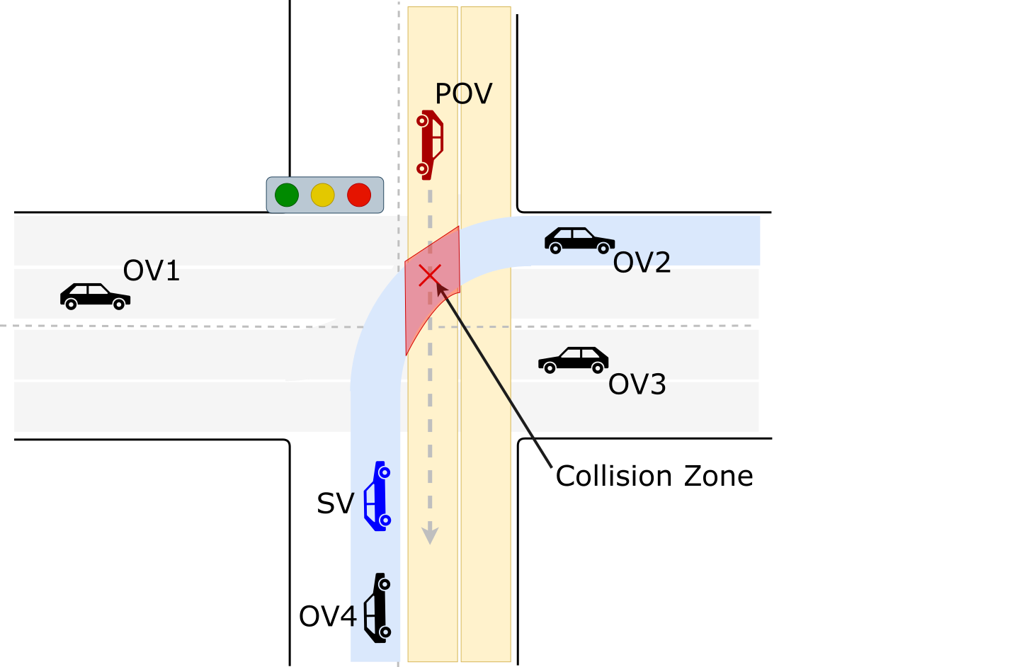
Figure 2: the intersection driving scenario, with the subject vehicle $\mathsf{SV}$ making a right turn and the principal other vehicle $\mathsf{POV}{}$ coming from the opposite

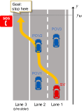
Figure 3: pull over

Another benefit of formalization by $\mathrm{dFHL}$ is compositional reasoning. In Floyd–Hoare logic, one can derive $\{A\}\,\alpha;\beta\,\{C\}$ (a property of composition $\alpha;\beta$) from $\{A\}\,\alpha\,\{B\}$ and $\{B\}\,\beta\,\{C\}$ (properties of components). Via similar compositionality in $\mathrm{dFHL}$, we devised in [HasuoEHDBKPZPYSIKSS23] a workflow in which a complex scenario is split into subscenarios, and RSS rules are derived in a divide-and-conquer manner.

As a case study, we derived an RSS rule for the pull over scenario (Fig. 3). It is a complex scenario with a goal that requires high-level maneuver planning. It is an important MRM, too, for an ADV exiting its ODD.

I-C Automated Derivation of RSS Rules for Intersections

Our goal in this paper is a formal framework for deriving RSS rules for intersection scenarios such as Fig. 3. This class of driving scenarios exhibit unique challenges; to cope with them, we introduce a new theory that extends $\mathrm{dFHL}$ and emphasizes automation, together with its implementation.

Intersection scenarios exhibit complex interaction between vehicles. This makes modeling hard: there are many “discrete modes” due to the interaction, making manual modeling effort error-prone. Desired here is a compositional modeling formalism where one can model each vehicle separately, a feature absent in [HasuoEHDBKPZPYSIKSS23]. Another challenge is in verification: many discrete modes lead to complex case distinction and proof complexity; therefore proof automation is highly desired.

Our answer to these challenges is hybrid control flow graphs (hCFGs) as a modeling formalism (Section III). They are to hybrid programs in [HasuoEHDBKPZPYSIKSS23] what control flow graphs are to usual imperative programs; we introduce a synchronization mechanism so that multiple hCFGs compose. For reasoning, we adapt $\mathrm{dFHL}$ and introduce the notion of Hoare annotation (Section V). We propose an automated reasoning algorithm, and present its implementation and experimental evaluation.

I-D Contributions

We present the first framework for deriving RSS rules and proving their safety for intersection scenarios. Our technical contributions are as follows. 1) We introduce the modeling formalism of hCFGs that enables compositional agent-wise modeling (Section III). Their semantics is via translation to hybrid programs [HasuoEHDBKPZPYSIKSS23]. 2) We introduce the reasoning formalism of Hoare annotations (Section V), an automated reasoning algorithm, and its implementation (Section VI). 3) We apply the above framework to the intersection situation in Section IV—it consists of the driving scenario Fig. 3 and a specific proper response $\alpha$—and let our implementation automatically derive an RSS condition $A$. 4) We experimentally evaluate the RSS rule $(A,\alpha)$.

I-E Organization, Notations and Terminologies

After reviewing $\mathrm{dFHL}$ [HasuoEHDBKPZPYSIKSS23] in Section II, we introduce hCFGs in Section III, with their composition and semantics. The intersection case study is given in Section IV. We go back to the general theory and introduce Hoare annotations in Section V. Our algorithm is given in Section VI; in Section VII is the experimental evaluation.

The cardinality of a set $X$ is denoted by $|X|$. The set of polynomials over a set $X$ of variables is denoted by $\mathbb{R}[X]$. The syntactic equality is denoted by $\equiv$. We let $[i,j]=\{i,i+1,\dotsc,j\}$ for integers $i,j$ such that $i\leq j$. The propositional constants $\mathsf{true},\mathsf{false}$ denote truth and falsehood, respectively.

By a driving scenario we refer to an environmental setting in which the subject vehicle $\mathsf{SV}$ drives. A driving situation is a combination of a driving scenario and $\mathsf{SV}$’s control strategy. The latter is typically some MRM (a proper response in RSS).

I-F Related and Future Work

Some RSS rules are implemented and offered as a library [GassmannOBLYEAA19IV]. However, its coverage of various driving scenarios seems limited. For example, [KarimiD22] reports that CARLA’s autopilot safeguarded by the RSS library exhibits dangerous behaviors in an intersection scenario. This is because the RSS rule used there is essentially the one in Section I-A and does not address the intersection scenario.

There are some extensions of RSS. Besides our formalized, compositional and goal-achieving one [HasuoEHDBKPZPYSIKSS23], they study 1) parameter selection for balancing safety and progress [KonigshofOSS22], 2) an empirical (not logical) safeguard layer in addition to RSS [OborilS21], 3) extension to unstructured traffic with vulnerable road users [PaschOGS21], and 4) swerves as evasive manoeuvres [deIacoSC20IV]. The formalization in [HasuoEHDBKPZPYSIKSS23] has been extended to verification of safety architectures, too [EberhartDHH23]. All these extensions are orthogonal to the formalized approach of the current work, leaving their integration as future work.

Some recent works formalize traffic rules in temporal logic, so that they can be effectively monitored [DBLP:conf/ivs/MaierhoferMA22, DBLP:conf/ivs/LinA22]. Rules are given externally in [DBLP:conf/ivs/MaierhoferMA22, DBLP:conf/ivs/LinA22], while our goal is to derive such rules and prove their safety.

An automated driving controller typically aims also at requirements other than safety (such as comfort). For this purpose, use of hierarchically structured human-interpretable rules is advocated in [VeerLCCP2023]. In our previous work [EberhartDHH23] we also investigated hierarchically structured RSS rules, this time for the purpose of graceful degradation of safety. Combination of [EberhartDHH23] and the current work will not be hard.

Formal verification of ADV decision making in intersections is studied in [ChouhanB20, SaraogluPJ22, Rajhans13PhD]. They all take model-checking approaches, unlike the current work that emphasizes theorem proving. The work [ChouhanB20] employs statistical model checking, where correctness guarantees are by sampling and thus not absolute. The work [SaraogluPJ22] abstracts away continuous dynamics, unlike our explicit modeling by ODEs. Rigorous and fine-grained verification is pursued in [Rajhans13PhD] where high-level decision making and low-level continuous dynamics are holistically analyzed by multi-model heterogeneous verification. It is not clear how this method generalizes to numerous variations of intersection scenarios (while their $\mathrm{dFHL}$ modeling will not be hard). More comparison is future work.

Rule-based decision making for intersection scenarios is proposed in [AksjonovK21], but it does not come with safety proofs. From the RSS point of view, the work is suggesting proper responses, for which safety-guaranteeing RSS conditions can be derived using our framework. Doing so is future work.

For intersection safety, statistical and learning-based approaches are actively pursued, e.g. [Gao0CWHXWW0K21]. They are different from our logical approach that allows rigorous safety proofs.

Formal verification of ADV safety is pursued in e.g. [RizaldiISA18, RoohiKWSL18arxiv, KrookSLFF19]. The works [RizaldiISA18, RoohiKWSL18arxiv] adopt much more fine-grained modeling compared to the current work and [HasuoEHDBKPZPYSIKSS23]; a price for doing so seems to be scalability and flexibility. The work [KrookSLFF19] makes discrete (and thus coarse-grained) modeling.

II PRELIMINARIES: HYBRID PROGRAMS AND THE PROGRAM LOGIC $\mathrm{dFHL}$

We review the logic $\mathrm{dFHL}$ (differential Floyd–Hoare logic), introduced in [HasuoEHDBKPZPYSIKSS23] for the purpose of 1) modeling driving situations as imperative programs (called hybrid programs), and 2) to reason about their goal achievement and safety. For the framework later in §III–V, $\mathrm{dFHL}$ is both a main inspiration and an important technical building block.

The following collects the definitions needed in this paper. Further details are found in [HasuoEHDBKPZPYSIKSS23].

II-A Hybrid Programs

[assertion] Let $V$ be a fixed set of variables. A term over $V$ is a rational polynomial $f\in\mathbb{Q}[V]$ on $V$. Assertions over $V$ are generated by the grammar

$$A,B\;::=\;\mathsf{true}\mid\mathsf{false}\mid e\sim f\mid A\land B\mid A\lor B\mid\lnot A\mid A\Rightarrow B$$

where $e$, $f$ are terms and $\sim\ \in\left\{{=,\leq,<,\neq}\right\}$.

The openness and closedness of an assertion can be naturally defined: $x\leq 2$ is closed while $1<x\land x\leq 2$ is neither open nor closed, for example. See [HasuoEHDBKPZPYSIKSS23].

Hybrid programs are a combination of usual imperative programs and differential equations for continuous dynamics.

Hybrid programs are defined by

$$\alpha,\beta\quad::=\quad \mathsf{skip}{}\mid\alpha;\beta\mid x\mathop{{:}{=}}e\mid\mathsf{if}\,(A)\,\{\alpha\}\,\mathsf{else}{}\,\{\beta\}\mid$$

$$\mathsf{while}\,(A)\,\{\alpha\}\mid\mathsf{dwhile}\,(A)\,\{\dot{\mathbf{x}}=\mathbf{f}\}.$$

Here $x\in V$ is a variable, $e$ is a term, and $A$ is an assertion. In $\mathsf{dwhile}\,(A)\,\{\dot{\mathbf{x}}=\mathbf{f}\}$, $\mathbf{x}$ and $\mathbf{f}$ are lists of the same length, respectively of (distinct) variables and terms, and we require that $A$ be an open assertion. We sometimes drop the braces in $\mathsf{dwhile}\,(A)\,\{\dot{\mathbf{x}}=\mathbf{f}\}$ for readability. A differential while clause $\mathsf{dwhile}\,(A)\,\{\dot{\mathbf{x}}=\mathbf{f}\}$ encodes the continuous dynamics according to a system $\dot{\mathbf{x}}=\mathbf{f}$ of ODEs; it executes until the guard condition $A$ is falsified. Openness of $A$ ensures that, if $A$ is falsified at some point, then there is the smallest time $t_{0}$ when it is falsified, at which time the command’s continuation (if any) starts to execute.

The syntax of hybrid programs is inspired by $\mathrm{dL}$ [Platzer18], but comes with significant changes. See [HasuoEHDBKPZPYSIKSS23] for comparison.

[semantics of hybrid programs] A store $\rho\colon V\to\mathbb{R}$ is a function from variables to reals. The value $\left\llbracket{e}\right\rrbracket_{\rho}$ of a term $e$ in a store $\rho$ is a real defined as usual by induction on $e$ (see for example [Winskel93, §2.2]). The satisfaction relation between stores $\rho$ and assertions $A$, denoted by $\rho\vDash A$, is also defined as usual (see [Winskel93, §2.3]).

A state is a pair $\langle{\alpha},{\rho}\rangle$ of a hybrid program and a store. The reduction relation $\to$ on states is defined as usual, using several rules found in [HasuoEHDBKPZPYSIKSS23] (see Section II-A later). A state $s$ reduces to $s^{\prime}$ if $s\to^{*}s^{\prime}$, where $\to^{*}$ is the reflexive transitive closure of $\to$. A state $s$ converges to a store $\rho$, denoted by ${s}\mathrel{\Downarrow}{\rho}$, if there exists a reduction sequence $s\to^{*}\langle{\mathsf{skip}},{\rho}\rangle$.

The state $\langle{\alpha},{\rho}\rangle$, where $\alpha\,\equiv\,\left(\,\mathsf{dwhile}\,(x>0)\,\{\dot{x}=-1\}\,;\;x\mathop{{:}{=}}x-1\right)$ and $\rho(x)=2$, can reduce 1) to $\langle{\alpha},{{\rho}[{x}\to{v}]}\rangle$ for any $v\in(0,2]$, 2) to $\langle{x\mathop{{:}{=}}x-1},{{\rho}[{x}\to{0}]}\rangle$, and 3) to $\langle{\mathsf{skip}},{{\rho}[{x}\to{-1}]}\rangle$. Only the last one corresponds to convergence (namely ${\langle{\alpha},{\rho}\rangle}\mathrel{\Downarrow}{{\rho}[{x}\to{-1}]}$).

II-B The Program Logic $\mathrm{dFHL}$

A Hoare quadruple is a quadruple $\left\{A\right\}~{}\alpha~{}\left\{B\right\}\colon{}S$ of three assertions $A$, $B$, and $S$, and a hybrid program $\alpha$. It is valid if, for all stores $\rho$ such that $\rho\vDash A$,

• there exists $\rho^{\prime}$ such that ${\langle{\alpha},{\rho}\rangle}\mathrel{\Downarrow}{\rho^{\prime}}$ and $\rho^{\prime}\vDash B$, and

• for all reduction sequences $\langle{\alpha},{\rho}\rangle\to^{*}\langle{\beta},{\rho^{\prime}}\rangle$, $\rho^{\prime}\vDash S$.

Hoare quadruples have safety conditions $S$ in addition compared to Hoare triples (see e.g. [Winskel93]). They specify safety properties which must hold throughout execution.

The semantics of Hoare quadruples (Section II-B) has some notable features such as accommodation of continuous dynamics and total correctness semantics. See [HasuoEHDBKPZPYSIKSS23] for details.

The logic $\mathrm{dFHL}$ has several derivation rules for Hoare quadruples. Many of them are standard Hoare logic rules (see e.g. [Winskel93]), extended in a natural manner to accommodate safety conditions. The rules for the $\mathsf{dwhile}$ construct come in two versions. One uses explicit closed-form solutions; this is the one we will use. The other uses differential (in)variants—formulated using Lie derivatives—that correspond to barrier certificates and Lyapunov functions in control theory. For space reasons, we refer to [HasuoEHDBKPZPYSIKSS23] for those derivation rules. They are sound, in that they only derive valid Hoare quadruples.

III HYBRID CONTROL FLOW GRAPHS (hCFGs)

III-A Formalization

A hybrid control flow graph (hCFG) is a tuple $\mathcal{G}=(L,\Sigma,E,V,\mathsf{Flow},\mathsf{Guard},\mathsf{Assign},l_{\mathsf{Init}},\mathsf{Final})$ where

• $L$ is a finite set of (control) locations;

• $\Sigma$ is a finite set of event names;

• $E\subseteq L\times\Sigma\times L$ is a finite set of edges that represent discrete “jumps” (we write $l\xrightarrow{a}l^{\prime}$ for $(l,a,l^{\prime})\in E$);

• $V$ is a finite set of real-valued variables;

• $\mathsf{Flow}$ is a function that associates, to each location $l\in L$, a system $\dot{\mathbf{x}}=\mathbf{f}$ of ODEs, where 1) $\mathbf{x}$ is the list (of length $|V|$) of all variables in $V$, and 2) $\mathbf{f}\in(\mathbb{Q}[V])^{|V|}$ is a list (of the same length) of polynomials over $V$;

• $\mathsf{Guard}$ is a function that associates, to each edge $e\in E$, its guard $A$ that is a closed assertion (Section II-A);

• $\mathsf{Assign}$ is a function that associates, to each edge $e\in E$ and a special label $\mathsf{Init}$ (designating initialization), a (possibly empty) list of assignment commands that are of the form $x\coloneqq f$ where $x\in V$ and $f\in\mathbb{Q}[V]$;

• $l_{\mathsf{Init}}\in L$ is an initial location; and

• $\mathsf{Final}\subseteq L$ is a set of final locations.

We further assume a fixed order between edges that go out of the same location. This is used later in Section III-B. hCFGs extend CFGs with flow dynamics, much like hybrid programs extend imperative programs [HasuoEHDBKPZPYSIKSS23]. They are also similar to hybrid automata (HA) [Henzinger96], with a key difference that invariants and guards in HA are replaced by guards.

$$\small\begin{array}[]{l}\raisebox{-0.5pt}{\scalebox{0.8}{ \leavevmode\hbox to12.75pt{\vbox to16.4pt{\text{[drawing]}}} }}\\ A_{l,i}=\mathsf{Guard}(e_{l,i})\end{array} l e_{l,n_{l}} l^{\prime}_{l,n_{l}} \vdots e_{l,1} l^{\prime}_{l,1} l e_{l,n_{l}} l^{\prime}_{l,n_{l}} \vdots e_{l,1} l^{\prime}_{l,1}$$ (3)

The semantics of guards in hCFGs is different from HA, too. Consider the location $l$ in 3, where $e_{l,1},\dotsc,e_{l,n_{l}}$ enumerate all outgoing edges from $l$, and $A_{l,i}$ are their guards.

Operationally, (the precise definition is later in Section III-B)

• the execution stays at $l$—exhibiting the flow dynamics specified by $\mathsf{Flow}(l)$—exactly as long as none of $A_{l,1},\dotsc,A_{l,n_{l}}$ is satisfied; and

• as soon as one of the guards is satisfied (say $A_{l,i}$), the $i$-th edge is taken and location jump occurs.

III-B Translation to Hybrid Programs and Formal Semantics

[hCFGs to hybrid programs] Let $\mathcal{G}$ be an hCFG as in Section III-A, where $L=\{l_{1},\dotsc,l_{n}\}$, $l_{1}=l_{\mathsf{Init}}$ and $\mathsf{Final}=\{l_{k+1},l_{k+2},\dotsc,l_{n}\}$. The hybrid program $[\mathcal{G}]$ is

$$\small\begin{array}[]{l}l\coloneqq l_{1}\,;\qquad\hfill\text{// setting program counter to $l_{1}$\;}\\ \mathsf{Assign}(\mathsf{Init})\,;\qquad\hfill\text{// initial assignment commands\;}\\ \mathsf{while}\,(l\not\in\mathsf{Final})\,\{\hfill\text{\qquad// until reaching a final location\;}\\ \quad\mathsf{if}(l=l_{1})\ \mathsf{then}\ \{B_{1}\}\\ \quad\mathsf{else}\ \mathsf{if}\ (l=l_{2})\ \mathsf{then}\ \{B_{2}\}\\ \quad\dotsc\\ \quad\mathsf{else}\ \mathsf{if}\ (l=l_{k})\ \mathsf{then}\ \{B_{k}\}\\ \}\\ \begin{array}[]{r}\text{where}\\ \text{$B_{i}$ is}\end{array}\left[\footnotesize\begin{array}[]{l}\mathsf{dwhile}\,(\lnot A_{l_{i},1}\land\cdots\land\lnot A_{l_{i},n_{l_{i}}})\,\{\;\mathsf{Flow}(l_{i})\;\}\,;\\ \mathsf{if}(A_{l_{i},1})\ \mathsf{then}\ \{\mathsf{Assign}(e_{l_{i},1});\;l:=l^{\prime}_{l_{i},1}\}\\ \mathsf{else}\ \mathsf{if}\ (A_{l_{i},2})\ \mathsf{then}\ \{\mathsf{Assign}(e_{l_{i},2});\;l:=l^{\prime}_{l_{i},2}\}\\ \mathsf{else}\ \mathsf{if}\ \dotsc\\ \mathsf{else}\ \mathsf{if}\ (A_{l_{i},n_{l_{i}}})\ \mathsf{then}\ \{\mathsf{Assign}(e_{l_{i},n_{l_{i}}});\;l:=l^{\prime}_{l_{i},n_{l_{i}}}\}\end{array}\right]\end{array}$$

We adopted the notation 3 in $B_{i}$. There, the $\mathsf{dwhile}$ construct in the first line executes the specified flow dynamics as long as $\lnot A_{l_{i},1}\land\cdots\land\lnot A_{l_{i},n_{l_{i}}}$ is true. Once we leave the flow dynamics, we take a transition $l_{i}\to l^{\prime}_{l_{i},j}$ whose guard $A_{l_{i},j}$ is satisfied; when there are multiple such, we use the fixed order of edges (assumed in Section III-A) to resolve the possible nondeterminism, in the way explicated in the $\mathsf{if}\ \cdots\mathsf{else}\ \mathsf{if}\ \cdots$ construct in $B_{i}$.

[semantics of hCFGs] Let $\mathcal{G}$ be an hCFG. Its operational semantics is defined to be that of the hybrid program $[\mathcal{G}]$, where the latter is defined in Section II-A.

III-C Networks of hCFGs

The following formalism enables compositional modeling. It is much like networks of timed automata (see e.g. [BengtssonY03]) although ours features richer interaction, as explained later.

[network of hCFGs] An open hCFG is defined in the same way as hCFGs (Section III-A), with the difference that 1) the flow dynamics $\mathsf{Flow}(l)\equiv(\dot{\mathbf{x}=\mathbf{f}})$ may not cover all variables in $V$ (that is, the length of the list $\mathbf{x}$ may be $<|V|$), and 2) it has no final locations specified.

A network of hCFGs is a tuple $\mathcal{N}=(\mathcal{G}^{(1)},\dotsc,\mathcal{G}^{(k)})$ of open hCFGs (these are called component hCFGs of $\mathcal{N}$) such that 1) their location sets $L^{(1)},\dotsc,L^{(k)}$ are disjoint, 2) they share the same set $V$ of variables, and 3) they satisfy so-called compatibility conditions, deferred to Section -A, requiring that there are no conflicts in the descriptions of dynamics in different hCFGs.

Intuitively, a variable can be changed (by $\mathsf{Flow}$ or $\mathsf{Assign}$) by only one component, but it can be seen (i.e. occur in guards) in multiple components. This “can’t change but can see” interaction—essential in modeling driving situations—is not present in networks of timed automata [BengtssonY03]. A consequence of this feature is that a component CFG does not have its own semantics: its behavior depends on variables changed by other components. This does not matter for our purpose (compositional modeling, not compositional verification).

The semantics of a network of hCFGs is defined by the synchronized product of component hCFGs. There are two modes of synchronization: by shared variables (in guards), and by shared events (in edge labels). Below is an informal definition; a formal definition is in Section -B. The semantics of a network $\mathcal{N}=(\mathcal{G}^{(1)},\dotsc,\mathcal{G}^{(k)})$ of hCFGs is defined to be the semantics (Section III-B) of its synchronized product $\mathcal{G}_{\mathcal{N},\mathsf{Final}}$ with a given set $\mathsf{Final}$ of final locations ($\mathsf{Final}$ is specified separately). The hCFG $\mathcal{G}_{\mathcal{N},\mathsf{Final}}$ is defined in a usual manner. Its location is a tuple $(l^{(1)},\dotsc,l^{(k)})$ of locations of components. When an event name $a$ is shared by multiple components, we require that all these components synchronize. The flow dynamics, guards, and assignment commands are defined by suitably joining those of components.

IV THE INTERSECTION SITUATION: MODELING

inline,caption=]use the new model Here we describe our hCFG modeling of the main case study, namely the intersection driving situation.

IV-A The Intersection Situation, Informally

inline,caption=](Ichiro) James, can you name the vehicles in the figure? I think you can call them OV1, …, OV4. The driving situation is illustrated in Fig. 3. There is an intersection with traffic lights, and the lights are green for the vertical road—both upwards and downwards—and they are red for the horizontal one. There may be many vehicles, but we assume that only the following two are relevant.

$\mathsf{SV}$

The subject vehicle making a right turn.

$\mathsf{POV}{}$

The principal other vehicle is driving straight downwards, potentially causing a collision with $\mathsf{SV}$.

The other vehicles in Fig. 3 are irrelevant, physically (far away) or by responsibility (red traffic light or behind $\mathsf{SV}$).

The problem of this case study is as follows. We focus on one specific minimum risk maneuver (MRM), namely for $\mathsf{SV}$ to stop as quickly as possible. We ask if this MRM is safe. In RSS terms (Section I-A), the problem is to compute an RSS condition for the max-brake proper response.

Note that this case study is only part of the safety analysis of the intersection scenario in Fig. 3. There are other conceivable proper responses, such as accelerating to leave the intersection quickly. For each such proper response, we can conduct a similar analysis to find its RSS condition. A catalogue of proper responses and their RSS conditions, obtained this way, can be used for the maneuver planning of $\mathsf{SV}$: we can choose a proper response whose RSS condition is true; we can use some preference if there are multiple such. This conditional combination of proper responses is what is done in [HasuoEHDBKPZPYSIKSS23, §IV-E].

We assume that $\mathsf{SV}$ and $\mathsf{POV}{}$ maintain their lanes (which we can confirm by their turn signals off); therefore only two lanes are relevant to us.

IV-B An hCFG Modeling

The intersection situation exhibits complex interaction between $\mathsf{SV}$ and $\mathsf{POV}{}$. Such interaction can be causal (if $\mathsf{SV}$ is in the collision zone then $\mathsf{POV}{}$ must act to avoid collision) or temporal ($\mathsf{SV}$ may enter the collision zone before $\mathsf{POV}{}$, after it, or simultaneously). We use a network of hCFGs (Section III-C) to deal with the complication.

(a) $\mathcal{G}^{\mathsf{SVPos}}$ for $\mathsf{SV}$’s position

(b) $\mathcal{G}^{\mathsf{SVVel}}$ for $\mathsf{SV}$’s velocity

(c) $\mathcal{G}^{\mathsf{SVTimer}}$ for $\mathsf{SV}$’s response time

(d) $\mathcal{G}^{\mathsf{POVPos}}$ for $\mathsf{POV}{}$’s position

(e) $\mathcal{G}^{\mathsf{POVVel}}$ for $\mathsf{POV}{}$’s velocity. Note that various events (such as $\mathsf{POVStartBraking}$) trigger the change of $\mathsf{POV}{}$’s acceleration, regulating its velocity

(f) $\mathcal{G}^{\mathsf{POVTimer}}$ for $\mathsf{POV}{}$’s response time

Figure 4: the network $\mathcal{N}^{\mathsf{int}}$ of hCFGs for the intersection situation, consisting of six open hCFGs; final locations are as in 4

Concretely, our model is the network of hCFGs presented in Fig. 4. We use the following variables and constants.

• The positions and velocities of $\mathsf{SV}$ and $\mathsf{POV}{}$ are expressed in the lane coordinates, for the lanes shown in Fig. 3. We use the variables $x_{\mathsf{SV}},x_{\mathsf{POV}{}},v_{\mathsf{SV}},v_{\mathsf{POV}{}}$ for them. $\mathsf{POV}{}$’s behavior has nondeterminism: it can accelerate, brake, or cruise, unless it brakes to avoid collision. We model two extremes, using the variables $x_{\mathsf{POV}{}}^{\mathsf{max}},x_{\mathsf{POV}{}}^{\mathsf{min}}$, etc.

• The region in which these two lanes intersect is called the collision zone ($\mathsf{CZ}$). $\mathsf{CZ}$ is expressed by intervals in the lane coordinates, namely by $[x_{\mathsf{SV}}^{\mathsf{CZStart}},x_{\mathsf{SV}}^{\mathsf{CZEnd}}]$ and $[x_{\mathsf{POV}{}}^{\mathsf{CZStart}},x_{\mathsf{POV}{}}^{\mathsf{CZEnd}}]$, respectively.

• The maximum braking rate $b>0$ is a constant.

• For dealing with the response time $\rho$ (that is a constant), $\mathsf{SV}$ and $\mathsf{POV}{}$ have their timer variables $t_{\mathsf{SV}},t_{\mathsf{POV}{}}$.

Let us go into each component open hCFG.

The components $\mathcal{G}^{\mathsf{SVPos}},\mathcal{G}^{\mathsf{POVPos}}$ describe the positions, with different locations ($\mathsf{SVBeforeCZ},\mathsf{SVInCZ}$, etc.) designating the vehicles’ (discrete) position relative to $\mathsf{CZ}$. The ODE for the flow dynamics stays the same in each component, where the values of $v_{\mathsf{SV}},v_{\mathsf{POV}{}}$ are governed by other components. Note that $\mathsf{POVInCZ}$ is modeled conservatively: it starts when the fastest possible $\mathsf{POV}{}$ reaches $\mathsf{CZ}$; it ends when the slowest possible leaves $\mathsf{CZ}$.

The components $\mathcal{G}^{\mathsf{SVVel}},\mathcal{G}^{\mathsf{POVVel}}$ describe the velocities. Here, we have multiple locations to accommodate different flow dynamics (i.e. different acceleration). The events $\mathsf{SVStartBraking},\mathsf{POVStartBraking}$ come with no explicit guards, but they are implicitly guarded by the conditions $t_{\mathsf{SV}}\geq\rho,t_{\mathsf{POV}{}}\geq\rho$ for the same events in the timer components $\mathcal{G}^{\mathsf{SVTimer}},\mathcal{G}^{\mathsf{POVTimer}}$. Recall from Section III-C that components must synchronize upon shared events.

The component $\mathcal{G}^{\mathsf{POVVel}}$ is more complex than $\mathcal{G}^{\mathsf{SVVel}}$ since two extreme $\mathsf{POV}{}$s may stop at different moments. It is semantically clear that the location $\mathsf{POVMinBrMaxSt}$ is vacuous. We include it so that the modeling is systematic; our reasoning algorithm indeed detects that it is vacuous.

The components $\mathcal{G}^{\mathsf{SVTimer}},\mathcal{G}^{\mathsf{POVTimer}}$ govern the timer variables. The one for $\mathsf{SV}$ ticks from the beginning, counting up to $\rho$, at which the event $\mathsf{SVStartBraking}$ is enabled in $\mathcal{G}^{\mathsf{SVTimer}}$, hence in $\mathcal{G}^{\mathsf{SVVel}}$ by synchronization. In contrast, the one for $\mathsf{POV}{}$ starts counting only when the event $\mathsf{SVEnterCZ}$ occurs, which must synchronize with the same event in $\mathcal{G}^{\mathsf{SVPos}}$. This way, $\mathcal{G}^{\mathsf{POVTimer}}$ starts ticking when it sees $\mathsf{SV}$ in $\mathsf{CZ}$.

Most of the component hCFGs are straightline and they may seem deterministic. Nevertheless, the whole system comes with nondeterminism due to the product construction—for example, at the initial state, the next event can be one of $\mathsf{SVEnterCZ}$, $\mathsf{POVEnterCZ}$, etc., depending on the values of variables.

We note that each component is simple and clearly presents its intuition. It is also easy to compare corresponding components for different vehicles, manifesting their similarities and differences. These features of hCFGs greatly aid explainability and accountability of the modeling process.

The final locations are defined as follows.

$$\small\begin{array}[]{l}\mathsf{Final}^{\mathsf{int}}\;:=\;\bigl{\{}\,(l^{\mathsf{SVPos}},\dotsc,l^{\mathsf{POVTimer}})\,\big{|}\\ \;l^{\mathsf{SVPos}}=\mathsf{SVAfterCZ}\lor l^{\mathsf{POVPos}}=\mathsf{POVAfterCZ}\\ \;\lor(l^{\mathsf{SVVel}}=\mathsf{SVStopped}\land l^{\mathsf{POVVel}}=\mathsf{POVBothSt})\,\bigr{\}}\end{array}$$ (4)

In all these cases there is no possibility of further collision, or the situation will no longer evolve.

V REASONING OVER hCFGs

[Hoare annotation] Let $\mathcal{G}$ be an hCFG in Section III-A. We adopt the notations in Section III-B for edges, etc.

A Hoare annotation $\gamma$ for $\mathcal{G}$ is a function that associates, to each location $l$ of $\mathcal{G}$, an assertion $\gamma(l)$ over $V$ (cf. Section II-A).

Let $S$ be an assertion, and $\mathsf{Unsafe}$ be a set of locations. A Hoare annotation $\gamma$ for $\mathcal{G}$ is valid under a safety condition $S$ and unsafe locations $\mathsf{Unsafe}$ if the following holds.

If $l\in\mathsf{Final}$, then the implication $\gamma(l)\Rightarrow S$ is valid.

If $l\in\mathsf{Unsafe}$, then $\gamma(l)\Rightarrow\mathsf{false}$ is valid.

Otherwise, let $l\in L\setminus(\mathsf{Final}\cup\mathsf{Unsafe})$ be a location that is not final nor unsafe; let its successors and guards denoted as in 3. Then there exist assertions $C_{l,1},\dotsc,C_{l,n_{l}}$ such that

• the Hoare quadruple

  $$\begin{array}[]{r}\Bigl{\{}C_{l,i}\Bigr{\}}\;\left({\scriptsize\begin{array}[]{l}\mathsf{dwhile}\,(\lnot A_{l,i})\,\{\\ \quad\mathsf{Flow}(l)\\ \}\end{array}}\right)\,\Bigl{\{}\,\gamma(l^{\prime}_{l,i})\,\bigl{[}\,\mathsf{Assign}(e_{l,i})\,\bigr{]}\,\Bigr{\}}\\ \qquad\quad\;:\;S\land\bigwedge_{j\in[1,n_{l}]\setminus\{i\}}\lnot A_{l,j}\end{array}$$ (5)

  is valid for each $i\in[1,n_{l}]$, where $\gamma(l^{\prime}_{l,i})\,\bigl{[}\,\mathsf{Assign}(e_{l,i})\,\bigr{]}$ is the assertion defined below, and

• the implication $\gamma(l)\Rightarrow C_{l,1}\lor\cdots\lor C_{l,n_{l}}$ is valid.

In 5, the assertion $\gamma(l^{\prime}_{l,i})\,\bigl{[}\,\mathsf{Assign}(e_{l,i})\,\bigr{]}$ is obtained from $\gamma(l^{\prime}_{l,i})$ by the substitution specified in $\mathsf{Assign}(e_{l,i})$. That is, letting $\mathsf{Assign}(e_{l,i})\equiv(x_{1}:=a_{1};\,\dotsc\,;\,x_{k}:=a_{k})$, we define $\gamma(l^{\prime}_{l,i})\,\bigl{[}\,\mathsf{Assign}(e_{l,i})\,\bigr{]}:\equiv\gamma(l^{\prime}_{l,i})\,[a_{k}/x_{k}]\,[a_{k-1}/x_{k-1}]\,\cdots\,[a_{1}/x_{1}].$

Some explanations are in order.

The basic idea is that $\gamma$ is an invariant: if true now, then it is true again in the next location. Precisely, if $\gamma(l)$ is true when $l$ is reached, then $\gamma(l^{\prime})$ should be true at the “jump” moment that the successor $l^{\prime}$ is reached. The definition is so that $\gamma$’s truth guarantees the (global) safety condition $S$ and the avoidance of unsafe locations. The condition $S$ is true throughout the flow dynamics, too, since $S$ is in the quadruple 5.

Therefore, for $\gamma$, we have that 1) it is an invariant, and 2) its truth guarantees truth of $S$ and avoidance of $\mathsf{Unsafe}$. Consequently, if $\gamma$ holds initially, then $S$ is true and $\mathsf{Unsafe}$ is avoided all the time. This is stated formally in Section V.

Branching according to guards requires some care (cf. 3); this is why we split $\gamma(l)$ into edge-wise preconditions $C_{l,i}$. The assertion $C_{l,i}$ ensures the following, since 5 is valid.

• The $i$-th edge $e_{l,i}$ is taken after the flow dynamics $\mathsf{Flow}(l)$ (due to $\bigwedge_{j\in[1,n_{l}]\setminus\{i\}}\lnot A_{l,j}$ in the safety condition of 5).

• Moreover, after taking the edge $e_{l,i}$ and executing the associated assignment $\mathsf{Assign}(e_{l,i})$, $\gamma(l^{\prime}_{l,i})$ holds at the successor $l^{\prime}_{l,i}$. This is because the assertion $\gamma(l^{\prime}_{l,i})[\mathsf{Assign}(e_{l,i})]$ in 5 is defined so that the quadruple $\bigl{\{}\,\gamma(l^{\prime}_{l,i})\,\bigl{[}\,\mathsf{Assign}(e_{l,i})\,\bigr{]}\,\bigr{\}}\;\mathsf{Assign}(e_{l,i})\;\bigl{\{}\,\gamma(l^{\prime}_{l,i})\,\bigr{\}}\;:\,S$ is valid (confirmed easily by the (Assign) rule in [HasuoEHDBKPZPYSIKSS23]).

In particular, when a non-final location $l$ has no outgoing edge, then $\gamma(l)=\mathsf{false}$, since there is no $C_{l,i}$ available.

The following result semantically justifies Section V. Its proof follows from the discussions so far. We need acyclicity of $\mathcal{G}$ for ensuring termination of $\mathcal{G}$’s execution (but not for safety). [semantic validity] Let $\gamma$ be a valid Hoare annotation for an hCFG $\mathcal{G}$ under $S$ and $\mathsf{Unsafe}$. Assume that $\mathcal{G}$ is acyclic, that is, that there is no cycle $l_{1}\xrightarrow{a_{1}}\cdots\xrightarrow{a_{k}}l_{k+1}$ in the graph $(L,E)$. Then the Hoare quadruple

$$\begin{array}[]{r}\Bigl{\{}\,\gamma(l_{\mathsf{Init}})\,\bigl{[}\,\mathsf{Assign}(\mathsf{Init})\,\bigr{]}\,\Bigr{\}}\;[\mathcal{G}]\;\Bigl{\{}\mathsf{true}\Bigr{\}}\\ \quad\colon\;S\land\bigwedge_{l_{i}\in\mathsf{Unsafe}}\lnot(l=l_{i})\end{array}$$ (6)

is valid in $\mathrm{dFHL}$. Here $[\mathcal{G}]$ is the translation in Section III-B, $l$ is the program counter variable in $[\mathcal{G}]$, and $\gamma(l_{\mathsf{Init}})\,[\mathsf{Assign}(\mathsf{Init})]$ is defined by substitution much like in Section V. ∎

END: AUX-PROOF

VI ALGORITHM AND IMPLEMENTATION

inline,caption=]say we use user annotation (which is trivial) Here we discuss our algorithm for finding an RSS condition. It operates on a given proper response that is modeled, together with its driving scenario, modeled as a network $\mathcal{N}$ of hCFGs. The algorithm’s outline is in Algorithm 1. The algorithm returns an assertion $A$ that makes the quadruple

$$\begin{array}[]{r}\bigl{\{}\,A\,\bigr{\}}\;[\mathcal{G}_{\mathcal{N},\mathsf{Final}}]\;\bigl{\{}\mathsf{true}\bigr{\}}\;\colon\;S\land\bigwedge_{l_{i}\in\mathsf{Unsafe}}\lnot(l=l_{i})\end{array}$$ (7)

valid. This $A$ is thought of as an RSS condition for the safety of the proper response. Our algorithm relies on Section V and symbolically synthesizes a valid Hoare annotation $\gamma$, which in turn yields a desired assertion as $\gamma(l_{\mathsf{Init}})\,[\mathsf{Assign}(\mathsf{Init})]$. The synthesis works backwards within the hCFG $\mathcal{G}_{\mathcal{N}}$, gradually defining $\gamma(l)$ for earlier $l$. We assume that the hCFG is acyclic.

Input: a network $\mathcal{N}$ of hCFGs, an assertion $S$, and sets $\mathsf{Final},\mathsf{Unsafe}$ of locations

Output: an assertion $A$ such that 7 is valid

1

2hCFG generation: generate the hCFG $\mathcal{G}_{\mathcal{N},\mathsf{Final}}$, following Section III-C

3Synthesizing $\gamma$, base case: for each unsafe location $l$, let $\gamma(l):=\mathsf{false}$; for each final location $l$ that is not unsafe, let $\gamma(l):=S$

4Synthesizing $\gamma$, step case: traverse the hCFG $\mathcal{G}_{\mathcal{N},\mathsf{Final}}$ backwards, finding $C_{l,i}$ in 5 and taking their disjunction to define $\gamma(l)$, as in Section V

return $\gamma(l_{\mathsf{Init}})\,[\mathsf{Assign}(\mathsf{Init})]$

Procedure 1 our algorithm

The most technical step is the step case of the synthesis of $\gamma$, where we search for a precondition $C_{l,i}$ that makes the quadruple 5 valid. To do so, we use the rules of $\mathrm{dFHL}$ [HasuoEHDBKPZPYSIKSS23]; note that most Hoare-style rules can be used for calculating weakest preconditions. To deal with the $\mathsf{dwhile}$ clauses, our implementation uses the rule (DWh-Sol) that exploits closed-form solutions. This makes the symbolic reasoning simpler than with the other rule (DWh) that requires differential (in)variants. The dynamics in our case study (Section IV) have closed-form solutions, too, given by quadratic formulas.

Our implementation is in Haskell, with approximately 1K LoC. It uses Z3 for checking validity of assertions, and Mathematica for solving ODEs.

VII EXPERIMENTS

Our implementation of Algorithm 1 successfully found a valid Hoare annotation $\gamma$, and hence an RSS condition, for the intersection case study (§IV). This RSS condition $A$ is an assertion over $x_{\mathsf{SV}},v_{\mathsf{SV}},x_{\mathsf{POV}{}},v_{\mathsf{POV}{}}$ (and parameters such as $b$) that, if true initially, guarantees a safe execution of the max-brake proper response.

We used the following safety specifications, identifying a collision as a joint occupancy of $\mathsf{CZ}$: $S^{\mathsf{int}}:=\mathsf{true}$ (no condition on the continuous dynamics); $\mathsf{Unsafe}^{\mathsf{int}}:=\bigl{\{}\,(l^{\mathsf{SVPos}},\dotsc,l^{\mathsf{POVTimer}})\,\big{|}\,l^{\mathsf{SVPos}}=\mathsf{SVInCZ}\land l^{\mathsf{POVPos}}=\mathsf{POVInCZ}\,\bigr{\}}$. The automated derivation took a couple of minutes, most of which was spent for validity checking by Z3. The synthesis of $\gamma$ was assisted by some user-provided assertions, although these assertions are straightforward (such as $v_{\mathsf{SV}}\geq 0\land x_{\mathsf{SV}}^{\mathsf{CZStart}}\leq x_{\mathsf{SV}}$ for the location $\mathsf{SVInCZ}$ in $\mathcal{G}^{\mathsf{SVPos}}$). Fully automatic synthesis (without assistance) should not be hard; we leave it as future work.

We conducted experiments to evaluate the RSS condition $A$ we obtained for the intersection situation. We posed the following research questions.

RQ1

Does the RSS condition $A$ indeed guarantee safety ($A$ true $\Rightarrow$ no collision)? This is theoretically guaranteed by Section V, but we want to experimentally confirm.

RQ2

Is $A$ not overly conservative? That is, when it is false ($A$ says there is risk), is there a real risk of collision?

Another question is about the ease of modeling. We believe that the compositional modeling in Section IV answers it positively.

To address the RQs, we implemented a simulator of the intersection situation (cf. Fig. 3), on which we conducted a number of simulations for different parameter values. The parameter space consists of the following.

• Initial values of positions and velocities of $\mathsf{SV}$ and $\mathsf{POV}{}$, chosen from the ranges $x_{\mathsf{SV}},x_{\mathsf{POV}{}}\in\{5,10,\dotsc,45\}[$\text{\,}\mathrm{m}\text{/}$]$ and $v_{\mathsf{SV}},v_{\mathsf{POV}{}}\in\{3,6,\dotsc,18\}[$\text{\,}\mathrm{m}\text{/}\mathrm{s}$]$. The numbers are in lane coordinates; positions are measured from $\mathsf{CZ}$’s center. (Note that some initial values are inevitably unsafe.)

• There is nondeterminism in $\mathsf{POV}{}$’s behavior, namely in what it does before it needs to brake (in the location $\mathsf{POVAccelerating}$ of Fig. 4). We consider $\mathsf{POV}{}$s that maintain the same acceleration rate $a_{\mathsf{POV}{}}$, and $a_{\mathsf{POV}{}}$ is chosen from $\{-5,-4,\dotsc,0,1,2\}[$\text{\,}\mathrm{m}\mathrm{/}\mathrm{s}^{2}$]$.

Note that the RSS condition $A$ is formulated in terms of (the initial values of) $x_{\mathsf{SV}},x_{\mathsf{POV}{}},v_{\mathsf{SV}},v_{\mathsf{POV}{}}$; it does not refer to $a_{\mathsf{POV}{}}$ since $A$ needs to guarantee safety for all possible $\mathsf{POV}{}$’s behavior. Therefore, we refer to a choice of the values of $x_{\mathsf{SV}},x_{\mathsf{POV}{}},v_{\mathsf{SV}},v_{\mathsf{POV}{}}$ as an instance; each simulation is run under an additional choice of the value of $a_{\mathsf{POV}{}}$.

As for constants, we used $b=$5\text{\,}\mathrm{m}\mathrm{/}\mathrm{s}^{2}$,a_{\mathrm{max}}=$2\text{\,}\mathrm{m}\mathrm{/}\mathrm{s}^{2}$$, and $\rho=$0.3\text{\,}\mathrm{s}\text{/}$$. In a simulation, $\mathsf{SV}$ executed the max-brake proper response (cruise for $\rho$ and brake at $b$); $\mathsf{POV}{}$ accelerated at $a_{\mathsf{POV}{}}$, braking when it sees $\mathsf{SV}$ in $\mathsf{CZ}$.

We ran 23,328 simulations, that is, 8 simulations (for different $\mathsf{POV}{}$ behaviors) for each of 2,916 instances. The simulation results are summarized in Table I, counting

• what we call RSS complying instances (i.e. in which the initial values of $x_{\mathsf{SV}},x_{\mathsf{POV}{}},v_{\mathsf{SV}},v_{\mathsf{POV}{}}$ satisfy the RSS condition $A$) vs. RSS non-complying ones, and

• what we call experimentally safe instances (i.e.  those whose eight simulations under different $\mathsf{POV}{}$ behaviors are all collision-free) vs. experimentally unsafe ones.

TABLE I: Safety, by RSS rules and by experiments

	RSS complying	RSS non-complying
Experimentally unsafe	0	558
Experimentally safe	2296	62

Furthermore, in Fig. 5, we present how many simulations exhibit a collision for each RSS non-complying instance. (There is no collision in RSS complying instances.)

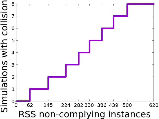
Figure 5: unsafe simulations per RSS non-complying instance

The experimental results yield the following answers to the research questions.

On RQ1, we confirmed experimentally that all RSS complying instances are safe. This is no surprise given the theoretical guarantee in Section V.

On RQ2, we see only a small number of false positive instances, i.e. those which are RSS non-complying but experimentally safe. According to Table I, the precision of the RSS condition is 90% and its recall is 100%. This high precision indicates that the RSS condition $A$, synthesized by our algorithm, is not overly conservative.

In Fig. 5, it is observed that the number of unsafe simulations vary greatly—depending on $\mathsf{POV}{}$’s behavior—and still the RSS condition $A$ successfully spots all unsafe instances.

Let us consider, for comparison, scenario-based testing methods for detecting unsafe instances. For such methods, spotting an unsafe instance with fewer unsafe simulations will be a challenge, since they have to find a rare $\mathsf{POV}{}$ behavior that causes a collision. In contrast, $\mathsf{POV}{}$ behaviors are universally quantified in our formal verification approach, in the form of the two extreme behaviors in Fig. 4. Therefore our approach can spot unsafe instances regardless of the rarity of collisions.

We note that an instance that is RSS non-complying with respect to $A$ may still be safe with respect to other proper responses than the max-brake one. See Section IV-A.

VIII Conclusions

Building on RSS [ShalevShwartzSS17RSS] and its formalization [HasuoEHDBKPZPYSIKSS23], we presented the first framework for automated formal verification of safety of intersection situations. The modeling formalism of hCFGs is suited to the multi-agent character of intersection situations; the reasoning formalism of Hoare annotations demonstrates the power of program logic. We believe this is an important step forward towards RSS’s coverage of a wide variety of real-world traffic scenarios, and hence towards the public acceptance of automated driving where its safety is mathematically proved.

-A Compatibility Conditions in Section III-C

• For each tuple $(l^{(1)},\dotsc,l^{(k)})$ of locations of the components (where $l^{(i)}\in L^{(i)}$ for each $i$), their flow dynamics has no conflicts, and moreover it is complete. That is, letting $\mathsf{Flow}(l^{(i)})\equiv(\dot{\mathbf{x}}^{(i)}=\mathbf{f}^{(i)})$, 1) if the same variable occurs in $\mathbf{x}^{(i)}$ and $\mathbf{x}^{(j)}$ with $i\neq j$, then the polynomials on their right-hand side (in $\mathbf{f}^{(i)},\mathbf{f}^{(j)}$) coincide, and 2) the union of $\mathbf{x}^{(1)},\dotsc,\mathbf{x}^{(k)}$ is the set $V$ of variables.

• Similarly, for each tuple $(e^{(1)},\dotsc,e^{(k)})$ of edges of the component hCFGs, there is no conflict in their assignment commands, meaning that $\mathsf{Assign}(e^{(1)}),\dotsc,\mathsf{Assign}(e^{(k)})$ have the same expressions on the right-hand side if the variable on the left-hand side is the same. We require the same compatibility for initial assignment commands, too.

-B Semantics of Networks of hCFGs, Formalized

The semantics of a network $\mathcal{N}=(\mathcal{G}^{(1)},\dotsc,\mathcal{G}^{(k)})$ of hCFGs is defined to be the semantics (Section III-B) of its synchronized product $\mathcal{G}_{\mathcal{N},\mathsf{Final}}$ with a given set $\mathsf{Final}$ of final locations. The latter is the hCFG defined below.

• Its locations are tuples $(l^{(1)},\dotsc,l^{(k)})$ of locations of components. Here $l^{(i)}\in L^{(i)}$ for each $i$.

• Its set $E_{\mathcal{N},\mathsf{Final}}$ of event names the union $E^{(1)}\cup\cdots\cup E^{(k)}$ of those of the components.

• Its set $V$ of variables is the one of all components.

• We have an edge $(l^{(1)},\dotsc,l^{(k)})\xrightarrow{a}(l^{\prime(1)},\dotsc,l^{\prime(k)})$ if 1) $l^{(i)}\xrightarrow{a}l^{\prime(i)}$ is an edge in $\mathcal{G}^{(i)}$ for each $i$ such that $a\in E^{(i)}$, and 2) $l^{(i)}=l^{\prime(i)}$ otherwise, i.e. for every $i$ such that $a\not\in E^{(i)}$. In this case, we say that the component edges $l^{(i)}\xrightarrow{a}l^{\prime(i)}$ enable the edge in $\mathcal{G}_{\mathcal{N},\mathsf{Final}}$. The intuition is that, if an event name $a$ is shared by multiple components, then all these components must synchronize in the event.

• Its flow dynamics at $(l^{(1)},\dotsc,l^{(k)})$ is the union of the flow dynamics of $l^{(1)},\dotsc,l^{(k)}$. By the compatibility condition (Section III-C), this union is well-defined and covers all variables in $V$, making $\mathcal{G}_{\mathcal{N},\mathsf{Final}}$ a (proper) hCFG.

• Its guard for an edge $(l^{(1)},\dotsc,l^{(k)})\xrightarrow{a}(l^{\prime(1)},\dotsc,l^{\prime(k)})$ is the conjunction of those guards associated with the enabling component edges $l^{(i)}\xrightarrow{a}l^{\prime(i)}$.

• Its assignment command for an edge in $\mathcal{G}_{\mathcal{N},\mathsf{Final}}$ is the concatenation of the assignment commands for the enabling component edges. There are no overriding assignments thanks to the compatibility condition (Section III-C). The initial assignment commands are defined similarly.

• Its initial location is the tuple $(l^{(1)}_{\mathsf{Init}},\dotsc,l^{(k)}_{\mathsf{Init}})$.

• Its set $\mathsf{Final}$ of final locations is specified separately. It is a set of locations, that is, $\mathsf{Final}\subseteq L^{(1)}\times\cdots\times L^{(k)}$.

References

- [1] S. Shalev-Shwartz, S. Shammah, and A. Shashua, “On a formal model of safe and scalable self-driving cars,” CoRR, vol. abs/1708.06374, 2017.
- [2] I. Hasuo, C. Eberhart, J. Haydon, J. Dubut, R. Bohrer, T. Kobayashi, S. Pruekprasert, X. Zhang, E. A. Pallas, A. Yamada, K. Suenaga, F. Ishikawa, K. Kamijo, Y. Shinya, and T. Suetomi, “Goal-aware RSS for complex scenarios via program logic,” IEEE Trans. Intell. Veh., vol. 8, no. 4, pp. 3040–3072, 2023.
- [3] I. Hasuo, “Responsibility-sensitive safety: an introduction with an eye to logical foundations and formalization,” CoRR 2206.03418, 2022.
- [4] C. Eberhart, J. Dubut, J. Haydon, and I. Hasuo, “Formal verification of safety architectures for automated driving,” in IV. IEEE, 2023, pp. 1–8.
- [5] F. Oboril and K. Scholl, “Rss: Pro-active risk mitigation for AV safety layers based on RSS,” in IV 2021. IEEE, 2021, pp. 99–106.
- [6] C. A. R. Hoare, “An axiomatic basis for computer programming,” Communications of the ACM, vol. 12, pp. 576–580, 583, 1969.
- [7] B. Gaßmann et al., “Towards standardization of AV safety: C++ library for responsibility sensitive safety,” in IV. IEEE, 2019, pp. 2265–2271.
- [8] A. Karimi and P. S. Duggirala, “Automatic generation of test-cases of increasing complexity for autonomous vehicles at intersections,” in ICCPS 2022. IEEE, 2022, pp. 1–11.
- [9] H. Königshof, F. Oboril, K. Scholl, and C. Stiller, “A parameter analysis on RSS in overtaking situations on german highways,” in IV 2022. IEEE, 2022, pp. 1081–1086.
- [10] F. Pasch, F. Oboril, B. Gassmann, and K. Scholl, “Vulnerable road users in structured environments with responsibility-sensitive safety,” in ITSC 2021. IEEE, 2021, pp. 270–277.
- [11] R. de Iaco, S. L. Smith, and K. Czarnecki, “Safe swerve maneuvers for autonomous driving,” in IV 2020, 2020, pp. 1941–1948.
- [12] S. Maierhofer, P. Moosbrugger, and M. Althoff, “Formalization of intersection traffic rules in temporal logic,” in IV, 2022, pp. 1135–1144.
- [13] Y. Lin and M. Althoff, “Rule-compliant trajectory repairing using satisfiability modulo theories,” in IV 2022. IEEE, 2022, pp. 449–456.
- [14] S. Veer, K. Leung, R. Cosner, Y. Chen, and M. Pavone, “Receding horizon planning with rule hierarchies for autonomous vehicles,” in ICRA, 2023.
- [15] A. P. Chouhan and G. Banda, “Formal verification of heuristic autonomous intersection management using statistical model checking,” Sensors, vol. 20, no. 16, 2020.
- [16] M. Saraoglu, J. Pintscher, and K. Janschek, “Designing a safe intersection management algorithm using formal methods,” IFAC-PapersOnLine, vol. 55, no. 14, pp. 22–27, 2022, proc. IAV 2022.
- [17] A. H. Rajhans, “Multi-model heterogeneous verification of cyber-physical systems,” Ph.D. dissertation, CMU, 2013.
- [18] A. Aksjonov and V. Kyrki, “Rule-based decision-making system for autonomous vehicles at intersections with mixed traffic environment,” in ITSC 2021. IEEE, 2021, pp. 660–666.
- [19] H. Gao et al., “Trajectory prediction of cyclist based on dynamic bayesian network and long short-term memory model at unsignalized intersections,” Sci. China Inf. Sci., vol. 64, no. 7, 2021.
- [20] A. Rizaldi, F. Immler, B. Schürmann, and M. Althoff, “A formally verified motion planner for autonomous vehicles,” in ATVA 2018, ser. Lecture Notes in Computer Science, vol. 11138, 2018, pp. 75–90.
- [21] N. Roohi, R. Kaur, J. Weimer, O. Sokolsky, and I. Lee, “Self-driving vehicle verification towards a benchmark,” CoRR 1806.08810, 2018.
- [22] J. Krook, L. Svensson, Y. Li, L. Feng, and M. Fabian, “Design and formal verification of a safe stop supervisor for an automated vehicle,” in ICRA, 2019, pp. 5607–5613.
- [23] A. Platzer, Logical Foundations of Cyber-Physical Systems. Springer International Publishing, 2018.
- [24] G. Winskel, The Formal Semantics of Programming Languages. MIT Press, 1993.
- [25] T. A. Henzinger, “The theory of hybrid automata,” in LICS 1996. IEEE Computer Society, 1996, pp. 278–292.
- [26] J. Bengtsson and W. Yi, “Timed automata: Semantics, algorithms and tools,” in Lect. on Concurrency and Petri Nets, Adv. in Petri Nets, ser. Lect. Notes in Comp. Sci., vol. 3098. Springer, 2003, pp. 87–124.