Impact-Aware Multi-Contact Balance Criteria

Abstract

Intentionally applying impacts while maintaining balance is challenging for legged robots. This study originated from observing experimental data of the humanoid robot HRP-4 intentionally hitting a wall with its right arm while standing on two feet. Strangely, violating the usual zero moment point balance criteria did not systematically result in a fall. To investigate this phenomenon, we propose the zero-step capture region for non-coplanar contacts, defined as the center of mass (CoM) velocity area, and validated it with push-recovery experiments employing the HRP-4 balancing on two non-coplanar contacts. To further enable on-purpose impacts, we compute the set of candidate post-impact CoM velocities accounting for frictional-impact dynamics in three dimensions, and restrict the entire set within the CoM velocity area to maintain balance with the sustained contacts during and after impacts. We illustrate the maximum contact velocity for various HRP-4 stances in simulation, indicating potential for integration into other task-space whole-body controllers or planners. This study is the first to address the challenging problem of applying an intentional impact with a kinematic-controlled humanoid robot on non-coplanar contacts.

I Introduction

Balancing under multiple, non-coplanar contacts is paramount for humanoid robots to shift weights, redistribute forces, and perform a wider range of tasks in real-world applications, e.g., [1]. Since many decades, constraining the so-called Zero-tilting Moment Point (ZMP) [2] within the support polygon is considered as an excellent dynamic balancing criteria when the robot stands on a flat surface, i.e., coplanar contacts. Recently, it has been extended to non-coplanar contact in [3]. However, we experimentally discovered that the ZMP-based criteria can be temporarily violated without necessarily resulting in loss of balance. As an example, the impact at the right palm in Fig. 1 enabled the ZMP jumped outside of the support polygon for a while, yet without leading to a fall.

It is challenging to predict the sudden change of ZMP induced by impact, even with knowledge of the contact velocity and location. Online implementation of robot control or planning call for low computationally-demanding impact models such as those based on rigid-body dynamics, e.g., [4]. These models can predict impact-induced change of velocities, not forces. As the ZMP is a measure of the resultant force, predicting its instantaneous change after an impact remains difficult.

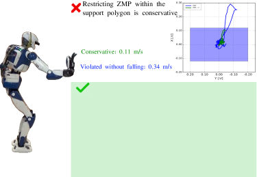
Figure 1: The peak impulsive force is 130 N according to the ATI sensor. Restricting the ZMP strictly within the support polygon leads to a conservative contact velocity of $0.11$ m/s (see video at https://youtu.be/TL34EWORwbU). Violating the ZMP balance criteria by increasing the contact velocity to $0.345$ m/s did not result in the robot falling (see video at https://youtu.be/FovQG6U448Q). The robot maintained balance during the experiments because the post-impact CoM velocities did not violate the zero-step capture region, located in the lower-right corner. Hence, to determine the maximum contact velocity, we propose restricting the entire set of candidate post-impact CoM velocities $\mathcal{X}_{{{\dot{{\text{\bf c}}}}}^{+}_{xy}}$ (shown as the blue polyhedron in the lower-left corner) within the zero-step capture region. Increasing the region’s size would lead to a higher contact velocity, as illustrated by the colored areas and the corresponding $\mathcal{X}_{{{\dot{{\text{\bf c}}}}}^{+}_{xy}}$ sets.

As an alternative to ZMP, [5] and [6] abstracted the robot dynamics with the linear inverted pendulum model (LIPM), and derived falling conditions according to the phase-plane analysis of the center-of-mass (CoM) dynamics. Their analysis is equivalent to constraining the CoM velocity by the zero-step capture region [7]. The impact in Fig. 1, which leads to a temporary violation of the ZMP-based criteria, did not enable the CoM velocity to cross the zero-step capture region. Thus, the comparison suggests that restricting CoM velocity can enable much less-conservative impacts than ZMP. Hence, we establish balance criteria employing CoM velocity to (1) maximize the intentional impact velocity; and (2) avoid the limitations of predicting post-impact ZMP. With respect to the problem defined in Sec. III-C, we summarize our contributions from two perspectives:

Handling non-coplanar contacts: In Sec. IV, we extend the zero-step capture region approach [5, 6, 7] to include non-coplanar contacts. To achieve this, we follow the derivation of the ZMP support area [3] and transform boundaries on ZMP to CoM velocities under the LIPM assumptions. Next, We project the high-dimensional CoM velocities (represented in the space of sustained contacts’ wrenches) onto a two-dimensional tangent plane of the inertial frame, while satisfying various constraints such as joint torque and velocity limits. The projection follows the ray-shooting algorithm presented in [8] and its 3D extension in [9].

Optimizing the entire set of post-impact CoM velocities: We assume that the robot is kinematic-controlled [10] with high stiffness in joint position or velocity, and that the impact is an instantaneous event occurring over a few milliseconds [11]. To approximate the set of candidate CoM velocities, we use convex polyhedra to be aware of all possible post-impact states, as shown in Fig. 1. By employing the vertices of the polyhedra as optimization variables, we present in Sec. V how to regulate the contact velocity with respect to the predicted sets of post-impact states.

Our study presents a solution enabling a kinematic-controlled legged robot to intentionally impact without losing balance. Our push-recovery experiment using the full-size humanoid robot HRP-4, employing two non-coplanar contacts on a 30-degree ramp and the ground, validates the zero-step capture region for non-coplanar contacts. By presenting an optimization-based approach to solve for maximum contact velocities for various HRP-4 stances, including kicking and pushing with non-coplanar contacts, our approach can be easily integrated into other whole-body controllers or planners, enabling legged robots to operate safely without loosing balance at impacts.

II Related Work

This section provides a brief overview of the relevant literature. In Sec. II-A, we discuss existing impact models in robotics. In Sec. II-B, we review the capture region and its extensions. Finally, in Sec. II-C, we discuss research on on-purpose impact tasks.

II-A Impact models

Several approaches have been proposed to model robotic impacts. In the late 1980s, [4] proposed modeling robotic impacts using the algebraic model based on Newton’s law of restitution and assumed frictionless contact. Model-based controllers or planners can seamlessly integrate this analytical model, according to [12, 13].

When the frictional impact is planar (two-dimensional), one can analytically compute the impulse by visiting the intersection points of the line of compression, the friction cone, and the two sliding directions. This strategy is known as Routh’s graphical approach [14] and is considered state-of-the-art impact mechanics [15, 16, 17, 18].

Impacts, can be described in 3D similarly to contact forces. In 3D, it is impossible to determine the post-impact tangential velocity, hence the tangential impulse, without numerical integrations [19, 20]. To the best of the author’s knowledge, frictional impact models in 3D are not well-validated for kinematic-controlled robots [11, 21]. Additionally, incorporating a numerical process (the impact model) into another numerical process (task-space optimization-based controller) is neither straightforward nor computationally efficient in terms of performance and robustness.

II-B Balance

II-B1 Coplanar contacts

Restricting the ZMP within the support polygon has been widely used for legged robots walking on flat terrains [22]. The ZMP balance criteria was also used in impact motions, e.g., hammering a nail [23], breaking a wooden piece with a Karate motion [24], or evaluating push-recovery motions [25, 26]. In the experiments conducted by [23, 24] the ZMP did not jump outside the support polygon. Thus, the impulses exerted by [23, 24] are not comparable to the example shown in Fig. 1.

ZMP amounts to a force measurement. Thus, predicting the instantaneous ZMP jump requires accurate impulse (momentum) prediction and proper estimation of the impact duration (time). Impact mechanics based on rigid-body dynamics can predict the impulse. Whereas, estimating the impact duration is not an easy task, due to the numerous unknown parameters, e.g., the Hertz contact stiffness [27, Sec. 4.1]. Therefore, in this paper, we rather favor an impact-aware balance criteria based on the CoM velocity.

If the divergent component of motion (DCM) [28] remains within the support polygon, the CoM stops and stay motionless. Thus the DCM is seen as the capture point [7]. In [5] and [6], the post-impact DCM is restricted within the support polygon, i.e., the capture region [7]. In this paper, we consider a fixed stance during impact, i.e., without modifying the sustained contacts. Hence, it is not comparable to the N-step capture region discussed in [7, 29].

II-B2 Non-coplanar contacts

We define the multi-contact wrench cone (MCWC) at the robot CoM as the Minkowski sum of the individual stable contact wrench cone (CWC) [30]. Employing the relation between ZMP and the resultant wrench, [30] projects the MCWC on a desired, two-dimensional plane to obtain the feasible ZMP support area. The projection follows the ray-shooting algorithm [8, 9], a simpler yet conservative approach is proposed in [31].

Given (1) MCWC, and (2) the relation between CoM velocity and ZMP, we can compute the CoM velocity area $\mathcal{X}_{[{\dot{{\text{\bf c}}}}_{xy}]}$. As long as the post-impact CoM velocity belongs to $\mathcal{X}_{[{\dot{{\text{\bf c}}}}_{xy}]}$, the sustained contacts can balance the robot.

Calculating the ZMP area ${\mathcal{X}_{[{\text{\bf z}}]}}$ assuming unlimited contact wrenches is not realistic, as it ignores kinematic and dynamic limitations. Hence, [3] reduced ${\mathcal{X}_{[{\text{\bf z}}]}}$ by making the LIPM assumptions, which include restricting the derivative of angular momentum to zero, maitaining a fixed CoM height, and fixing gravitational direction acceleration. More recently, [32] further improved ${\mathcal{X}_{[{\text{\bf z}}]}}$ by considering joint torque limits.

Note that we compute the full zero-step capture region rather than checking the zero-step capturability of a given stance [33], i.e., predicting the fall given the particular contact configurations, CoM position and velocity without computing the boundaries of the zero-step capture region.

II-C On-purpose impact tasks

Dynamic walking frequently exerts impacts as impact-less reference trajectories are challenging to generate and inefficient to execute [22]. State-of-the-art ZMP or DCM based walking control design ignores impact dynamics, e.g., see the examples by [34, 35]. The proposed criteria can enable far-less conservative impact motion, e.g., kicking velocities. Therefore, we can complement a whole-body controller [36], or a planner [37], to generate impact motions or balance behaviors that drastically change the centroidal momenta in a short time.

III Problem Formulation

We formulate our research problem with three steps. First, in Sec. III-A we introduce the mathematical tools to be used throughout the paper. Second, in Sec. III-B we use the phase portrait to analyze why the impact experiments shown in Fig. 1 did not lead to a fall. Then, in Sec. III-C we briefly state the research problem.

III-A Mathematical preliminaries

We will define the ZMP, the relationship between the ZMP and the CoM acceleration, and the linear inverted pendulum model (LIPM).

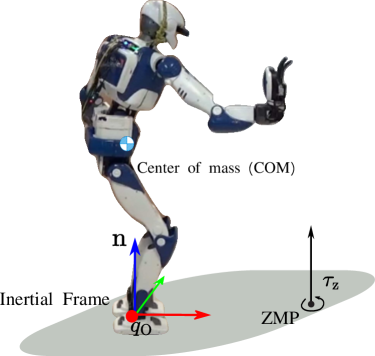
Figure 2: At the ZMP, the torque (black arrow) of the resultant contact wrench $\boldsymbol{\tau}_{{\text{\bf z}}}$ aligns with the normal vector n, which is the Z axis (blue arrow) of the inertial frame.

In Fig. 2, we define the inertial frame $\mathcal{F}_{\text{O}}$ whose origin $\boldsymbol{q}_{\text{O}}$ locates under the CoM, i.e., ${\text{\bf c}}_{x,y}=[0,0]^{\top}$.

Suppose the robot has ${\text{m}_{\text{sc}}}$ sustained contacts, we align the orientations of all the forces and wrenches according to the inertial frame. For instance, if the $i$-th contact wrench ${{}^{i}\boldsymbol{W}_{i}}$ is represented in the local frame, we represent ${{}^{i}\boldsymbol{W}_{i}}$ using the inertial frame’s orientation as:

$$\boldsymbol{W}_{i}=\begin{bmatrix}R_{i\text{O}}&0\\ 0&R_{i\text{O}}\end{bmatrix}{{}^{i}\boldsymbol{W}_{i}}$$

where $R_{i\text{O}}$ denotes the rotation from the $i$th contact frame $\mathcal{F}_{i}$ to the inertial frame $\mathcal{F}_{\text{O}}$.

Hence, we can compute the resultant wrench ${\boldsymbol{W}_{\text{O}}}$ at the origin of the inertial frame $\boldsymbol{q}_{\text{O}}$ as:

$${{\boldsymbol{W}_{\text{O}}}=\begin{bmatrix}{\boldsymbol{f}_{\text{O}}}\\ {\boldsymbol{\tau}_{\text{O}}}\end{bmatrix}={\mathds{1}_{\boldsymbol{W}}}\boldsymbol{W}=\underbrace{\begin{bmatrix}{\mathds{1}_{1}}&{\mathds{1}_{2}}&\ldots&{\mathds{1}_{{\text{m}_{\text{sc}}}}}\end{bmatrix}}_{{\mathds{1}_{\boldsymbol{W}}}\in\mathbb{R}^{6\times 6{\text{m}_{\text{sc}}}}}\underbrace{\begin{bmatrix}\boldsymbol{W}_{1}\\ \vdots\\ \boldsymbol{W}_{{\text{m}_{\text{sc}}}}\end{bmatrix}}_{\boldsymbol{W}\in\mathbb{R}^{6{\text{m}_{\text{sc}}}\times 1}}.}$$ (1)

The matrix ${\mathds{1}_{\boldsymbol{W}}}$ horizontally collects ${\text{m}_{\text{sc}}}$ blocks:

$${\mathds{1}_{i}}=\begin{bmatrix}\mathds{1}&0\\ \overrightarrow{\boldsymbol{q}_{\text{O}}\boldsymbol{p}_{i}}\times&\mathds{1}\end{bmatrix}\in\mathbb{R}^{6\times 6},\quad\text{for}\quad i=1,\ldots,{\text{m}_{\text{sc}}},$$

where $\mathds{1}\in\mathbb{R}^{3\times 3}$ denotes the identity matrix. The vector $\overrightarrow{\boldsymbol{q}_{\text{O}}\boldsymbol{p}_{i}}=\boldsymbol{\boldsymbol{p}_{i}}-\boldsymbol{\boldsymbol{q}_{\text{O}}}$ connects a contact point $\boldsymbol{p}_{i}$ to the origin $\boldsymbol{q}_{\text{O}}$ of the inertial frame. Thus, $\overrightarrow{\boldsymbol{q}_{\text{O}}\boldsymbol{p}_{i}}\times$ computes the resultant torque for a given sustained contact’s force.

III-A1 ZMP

Given a unit vector n, the Zero-tilting Moment Point (ZMP) [2, 3, 38] denotes the point where the torque of the resultant contact wrench $\boldsymbol{\tau}_{{\text{\bf z}}}$ aligns with n, see Fig. 2:

$${\text{\bf n}\times\boldsymbol{\tau}_{{\text{\bf z}}}=0.}$$ (2)

Computing the resultant wrench and the expansion of the vector triple product, we can define the ZMP as:

$${\text{\bf z}}=\frac{\text{\bf n}\times{\boldsymbol{\tau}_{\text{O}}}}{{\text{\bf n}}^{\top}{\boldsymbol{f}_{\text{O}}}}+d_{{\text{\bf z}}}\frac{{\boldsymbol{f}_{\text{O}}}}{{\text{\bf n}}^{\top}{\boldsymbol{f}_{\text{O}}}},$$ (3)

where we leave the detailed derivaiton in Appendix -F. If we assume that the scalar $d_{{\text{\bf z}}}={\boldsymbol{n}}^{\top}{\text{\bf z}}=0$, which means z belongs to the surface with the origin $\boldsymbol{q}_{\text{O}}$ and the surface normal $\boldsymbol{n}$, we have the simpler definition:

$${{\text{\bf z}}=\frac{\text{\bf n}\times{\boldsymbol{\tau}_{\text{O}}}}{{\text{\bf n}}^{\top}{\boldsymbol{f}_{\text{O}}}}.}$$ (4)

III-A2 CoM acceleration and ZMP

According to the derivation in Appendix -D, the CoM acceleration ${\ddot{{\text{\bf c}}}}$ depends on the ZMP z and angular momentum’s derivative $\dot{\mathcal{L}}$:

$${\ddot{{\text{\bf c}}}}=\boldsymbol{g}+\frac{\dot{\mathcal{L}}\times\text{\bf n}}{\text{m}(0pt{{\text{\bf c}}}-0pt{{\text{\bf z}}})}+\frac{{\text{\bf n}}^{\top}({\ddot{{\text{\bf c}}}}-\boldsymbol{g})\overrightarrow{{\text{\bf c}}{\text{\bf z}}}}{0pt{{\text{\bf c}}}-0pt{{\text{\bf z}}}}.$$ (5)

III-A3 The LIPM model

The LIPM model [5, 39] simplifies the whole-body dynamics (5) with two assumptions:

1. The vertical CoM acceleration is zero:

   $${\text{\bf n}}^{\top}{\ddot{{\text{\bf c}}}}=0.$$ (6)

2. The angular momentum about the CoM is fixed:

   $$\dot{\mathcal{L}}=0.$$ (7)

Substituting (6) and (7), we can simplify (5) to:

$${{\ddot{{\text{\bf c}}}}=\boldsymbol{g}+\frac{g}{0pt{{\text{\bf c}}}-0pt{{\text{\bf z}}}}({\text{\bf c}}-{\text{\bf z}}),}$$ (8)

where the detailed derivation is left in Appendix -E. If we project ZMP on the ground surface, i.e., $0pt{{\text{\bf z}}}=0$, and define the pendulum constant $\text{w}=\sqrt{\frac{g}{{\text{\bf c}}_{z}}}$, the planar components of (8) writes:

$${{\ddot{{\text{\bf c}}}}=\text{w}^{2}({\text{\bf c}}-{\text{\bf z}}).}$$ (9)

III-B Problem analysis

Choosing the state variable $\boldsymbol{x}=[{\text{\bf c}}_{x},{\dot{{\text{\bf c}}}}_{x}]^{\top}$, the state-space form of the LIPM dynamics (9) along the sagittal direction writes:

$$\begin{bmatrix}{\dot{{\text{\bf c}}}}_{x}\\ {\ddot{{\text{\bf c}}}}_{x}\end{bmatrix}=\begin{bmatrix}0&1\\ \text{w}^{2}&0\end{bmatrix}\begin{bmatrix}{\text{\bf c}}_{x}\\ {\dot{{\text{\bf c}}}}_{x}\end{bmatrix}+\begin{bmatrix}0\\ -\text{w}^{2}\end{bmatrix}{\text{\bf z}}_{x}.$$ (10)

The phase portrait of (10) in Fig. 3 shows the stable standing region [5, 40]:

$${\mathcal{X}_{\text{ssr}}}\vcentcolon=\{{{\text{\bf c}}_{x}+\frac{\dot{{\text{\bf c}}}_{x}}{\text{w}}}:\underline{{\text{\bf z}}_{x}}\leq{{\text{\bf c}}_{x}+\frac{\dot{{\text{\bf c}}}_{x}}{\text{w}}}\leq\overline{{\text{\bf z}}_{x}}\},$$ (11)

where the ZMP is limited by: ${\text{\bf z}}_{x}\in[\underline{{\text{\bf z}}_{x}},\overline{{\text{\bf z}}_{x}}]$.

For the HRP-4 stance in Fig. 1, we place the inertial frame’s origin $\boldsymbol{q}_{\text{O}}$ under the CoM, i.e., the CoM coordinates is: ${\text{\bf c}}=[0,0,0.78]$ m. Thus, substituting ${\text{\bf c}}_{x}=0$ into (11) simplifies ${\mathcal{X}_{\text{ssr}}}$ as:

$${\mathcal{X}_{\text{ssr}}}\vcentcolon=\{\frac{\dot{{\text{\bf c}}}_{x}}{\text{w}}:\underline{{\text{\bf z}}_{x}}\leq\frac{\dot{{\text{\bf c}}}_{x}}{\text{w}}\leq\overline{{\text{\bf z}}_{x}}\}.$$

Given ${\text{\bf c}}_{z}=0.78$ m, $g=\text{9.81}$ m/s², and ${\text{\bf z}}\in[-0.13,0.13]\leavevmode\nobreak\ m$, we can find the bounds: $\dot{{\text{\bf c}}}_{x}\in[-0.4608,0.4608]$ m/s. Thus, the two intersection points $[0,0.4608]$, $[0,-0.4608]$ in Fig. 3 (between the green vertical line and the ${\mathcal{X}_{\text{ssr}}}$) defines the interval, within which the CoM velocity can converge back to the origin.

Thus, despite the contact velocity $0.345$ m/s violated the ZMP-based criteria as shown in Fig. 1, it cannot cause a fall. Because the post-impact CoM velocity $-0.16$ m/s in Fig. 4 is within the interval $[-04608,0.4608]$ m/s.

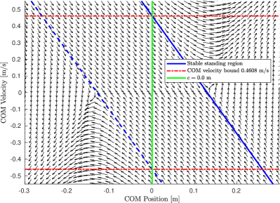
Figure 3: Simulation of the phase portrait of the LIPM dynamics (10) for the HRP-4 stance in Fig. 1, following [5]. The ZMP is saturated within the interval $[-0.13,0.13]$ m, and the CoM height is $0.78$ m.

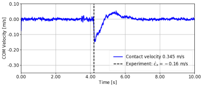
Figure 4: The CoM velocity ${\dot{{\text{\bf c}}}}_{x}$ at the impact time (indicated by the black dashed line) for the HRP-4 stance in Fig. 1 was within the analytical bound: $-0.16$ m/s $\in[-0.4608,0.4608]$ m/s.

However, the phase-portrait analysis in Fig. 3 has limitations: (1) the stable standing region ${\mathcal{X}_{\text{ssr}}}$ only applies in one direction, e.g., the sagittal direction; (2) the robot is restricted to coplanar contacts; and (3) intentional impacts are not considered. Hence, we formulate our research problem in the next subsection.

III-C Problem statement

Problem 1

We adopt the following assumptions for an intentional impact task:

1. The robot joint configurations $\mathbf{q}\in\mathbb{R}^{(n+6)}$, $\mathbf{\dot{q}}\in\mathbb{R}^{(n+6)}$ are known (measured or observed);

2. Prior to the impact, the robot’s initial multi-contact configuration is balanced (in theory this condition is conservative and can be relaxed).

3. The robot is high-stiffness controlled either in joint velocity or position, i.e., kinematic-controlled. It should be noted that robots with a different joint-control mode, such as a pure-torque controlled humanoid robot TORO, may behave differently during impact events.

4. There are ${\text{m}_{\text{sc}}}$ sustained non-coplanar rigid contacts with known friction coefficients;

5. We can approximate any of the sustained contacts’ geometric shape with a rectangle;

6. The robot controller can timely detect the collision, and pull back the end-effector without exerting additional impulses.

7. The impact does not break the sustained contacts during the impact event, which typically lasts for dozens of 40 ms in our previous experiments [10] (this condition can indeed be enforced by limiting the impact direction and intensity).

A task planner, or a human operator, typically provides a reference contact relative velocity $\boldsymbol{v}^{\text{ref}}\in\mathbb{R}^{3}$ for a given end-effector, e.g., the right palm in Fig. 5 is asked to impact along the yellow-arrow’s direction. However, when the reference velocity $\boldsymbol{v}^{\text{ref}}$ is too high it can lead to loosing balance and subsequent fall; the question is how to determine the maximum tracking velocity that does not cause falls.

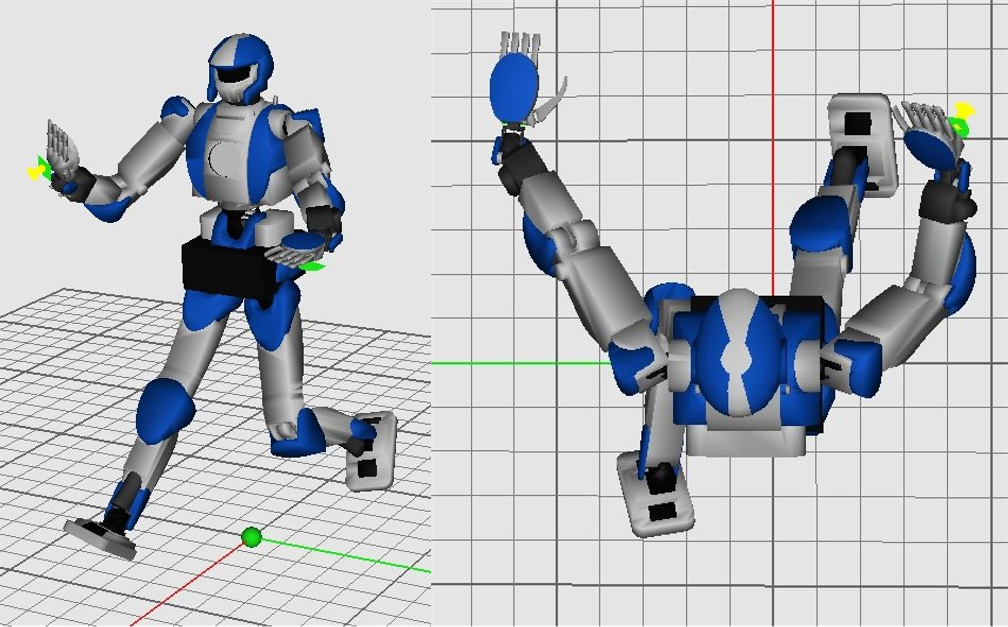
Figure 5: Side (left) and top (right) views of the HRP-4 robot with two non-coplanar contacts, i.e., two feet contacts with friction coefficient $0.7$. The robot applies impact with the right palm, as indicated by the yellow arrow.

$\blacksquare$

Controllers designed to be impact-aware, such as the one described in [41], take into account the frictional impact dynamics. Being able to predict the post-impact states, these controllers can use an impact event as a controlled process for various purposes, e.g., kicking or hammering. Therefore, we treat the impact as an instantaneous event that injects a predictable amount of impulse into the CoM dynamics and address Problem 1 in two steps:

1. Given the sustained contacts and joint configurations, we compute the CoM velocity area $\mathcal{X}_{[{\dot{{\text{\bf c}}}}_{xy}]}$ in Sec. IV. As long as ${{\dot{{\text{\bf c}}}}}^{+}_{xy}\in\mathcal{X}_{[{\dot{{\text{\bf c}}}}_{xy}]}$ after the impact, the robot can balance despite the impulse;

2. In Sec. V, we compute the set of post-impact CoM velocities $\mathcal{X}_{{{\dot{{\text{\bf c}}}}}^{+}_{xy}}$, and formulate novel inequality constraints to guarantee that $\mathcal{X}_{{{\dot{{\text{\bf c}}}}}^{+}_{xy}}\subseteq\mathcal{X}_{[{\dot{{\text{\bf c}}}}_{xy}]}$.

IV The CoM Velocity Area

After an impact event, the robot can balance utilizing the sustained contacts as long as the CoM velocity is within a specific range, which we refer to as the CoM velocity area. We present the CoM velocity area in three subsections. In Sec. IV-A, we summarize the set of resultant wrench $\mathcal{X}_{{\boldsymbol{W}_{\text{O}}}}$ at the origin of the inertial frame. In Sec. IV-B, we derive boundaries of the set of CoM velocities $\mathcal{X}_{[{\dot{{\text{\bf c}}}}_{xy}]}$, that can be balanced according to $\mathcal{X}_{{\boldsymbol{W}_{\text{O}}}}$. Finally, in Sec. IV-C, we project the high-dimensional-represented set $\mathcal{X}_{[{\dot{{\text{\bf c}}}}_{xy}]}$ onto the two-dimensional tangent plane of a humanoid robot following [3, 8].

IV-A The set of resultant wrenches

Given ${\text{m}_{\text{sc}}}$ sustained contact wrenches $\boldsymbol{W}\in\mathbb{R}^{6{\text{m}_{\text{sc}}}\times 1}$ in Sec. IV-A1, we constrain the resultant wrench at the inertial frame’s origin $\boldsymbol{q}_{\text{O}}$ according to limited actuation torques in Sec. IV-A2, and the LIPM assumptions in Sec. IV-A3.

IV-A1 Contact Wrench Cone

A sustained contact wrench $\boldsymbol{W}_{i}\in\mathbb{R}^{6}$ fulfills the Coulumb’s friction cone, has a limited torque, and does not slip. Assuming a rectangular contact area, Caron et al. [30] collected the three conditions into a half-space representation:

$${\mathcal{X}_{\boldsymbol{W}_{i}}\vcentcolon=\{\boldsymbol{W}_{i}\in\mathbb{R}^{6}:\text{C}_{i}\boldsymbol{W}_{i}\leq 0\},\quad\text{for }i=1,\ldots,{\text{m}_{\text{sc}}},}$$ (12)

where the details of $\text{C}_{i}\in\mathbb{R}^{16\times 6}$ are available in Appendix -F.

IV-A2 Limited actuation torques

According to the Newton’s third law, the sustained contact wrenches $\boldsymbol{W}\in\mathbb{R}^{6{\text{m}_{\text{sc}}}\times 1}$ are subject to the joint actuator torques limits $\text{B}\underline{\boldsymbol{\tau}}\leq\text{B}\overline{\boldsymbol{\tau}}\leq\text{B}\overline{\boldsymbol{\tau}}$. Thus, we re-formulate the equations of motion to restrict the sustained contacts’ wrenches $\boldsymbol{W}$ accordingly:

$${\underbrace{\begin{bmatrix}-{J}^{\top}\\ {J}^{\top}\end{bmatrix}}_{A}\boldsymbol{W}\leq\underbrace{\begin{bmatrix}\text{B}\overline{\boldsymbol{\tau}}-\text{M}\mathbf{\ddot{q}}-\mathbf{N}\\ -\text{B}\underline{\boldsymbol{\tau}}+\text{M}\mathbf{\ddot{q}}+\mathbf{N}\end{bmatrix}}_{B}.}$$ (13)

The detailed definition of $J,\text{M},\mathbf{N},\text{B}$ are left in (42) as part of Appendix -G.

IV-A3 LIPM Assumptions

To enforce the LIPM assumptions (6) and (7), we choose to constrain the resultant wrench ${\boldsymbol{W}_{\text{O}}}=[{\boldsymbol{f}_{\text{O}}}^{\top},{\boldsymbol{\tau}_{\text{O}}}^{\top}]^{\top}$.

1. For the zero vertical CoM acceleration assumption (6), we restrict the resultant force ${\boldsymbol{f}_{\text{O}}}$:

   $${\text{\bf n}}^{\top}{\boldsymbol{f}_{\text{O}}}=\text{m}g,$$ (14)

   where we use the scalar $\text{m}g$ instead of $\text{m}\boldsymbol{g}$. The gravity $\boldsymbol{g}$ takes the opposite sign of the $z$-axis of the inertial frame $\text{\bf n}=[0,0,1]^{\top}$, i.e., ${\boldsymbol{g}}^{\top}\text{\bf n}=-\text{9.81}$.

2. For the fixed angular momentum assumption (7), we restrict the resultant torque at the CoM $\boldsymbol{\tau}_{{\text{\bf c}}}$ according to [3]:

   1. Parallel to the Z axis $\text{\bf n}=[0,0,1]^{\top}$ of the inertial frame $\mathcal{F}_{\text{O}}$:

      $$\text{\bf n}\times\boldsymbol{\tau}_{{\text{\bf c}}}=0.$$ (15)

   2. Zero torque about n:

      $${\text{\bf n}}^{\top}\boldsymbol{\tau}_{{\text{\bf c}}}=0.$$ (16)

We re-formulate (14-16) in a matrix form (17). The detailed steps are left in Appendix -H.

$$\begin{bmatrix}0pt{{\text{\bf c}}}\cdot\mathds{1}&\text{\bf n}\times\\ -(\text{\bf n}\times{\text{\bf c}})^{\top}&\text{\bf n}^{\top}\end{bmatrix}\begin{bmatrix}{\boldsymbol{f}_{\text{O}}}\\ {\boldsymbol{\tau}_{\text{O}}}\end{bmatrix}=\begin{bmatrix}\text{m}g{\text{\bf c}}\\ 0\end{bmatrix}.$$ (17)

Thus, we summarize the set of resultant wrenches at the inertial frame’s origin as:

$${\mathcal{X}_{{\boldsymbol{W}_{\text{O}}}}\vcentcolon=\{{\boldsymbol{W}_{\text{O}}}\in\mathbb{R}^{6}:{\boldsymbol{W}_{\text{O}}}\text{\leavevmode\nobreak\ fulfills \eqref{eq:angular_momentum_assumption_constraint} }\}.}$$ (18)

IV-B Boundaries of the balancable CoM velocity set

We denote the set of CoM velocities $\mathcal{X}_{[{\dot{{\text{\bf c}}}}_{xy}]}$, within which the robot can stablize the CoM with the sustained contacts, i.e., the set of resultant wrenches $\mathcal{X}_{{\boldsymbol{W}_{\text{O}}}}$.

By fixing the inertial frame’s origin $\boldsymbol{q}_{\text{O}}$ under the CoM, we can simplify the stable standing region ${\mathcal{X}_{\text{ssr}}}$ by substituting ${\text{\bf c}}_{x,y}=[0,0]^{\top}$ into (11):

$${\mathcal{X}_{\text{ssr}}}\vcentcolon=\{{\dot{{\text{\bf c}}}_{x,y}}:\text{w}\underline{{\text{\bf z}}}\leq{\dot{{\text{\bf c}}}_{x,y}}\leq\text{w}\overline{{\text{\bf z}}}\}.$$

Thus, at the boundary of the set $\mathcal{X}_{{\dot{{\text{\bf c}}}}_{xy}}$, the planar CoM velocity ${\dot{{\text{\bf c}}}}_{xy}$ and ZMP ${\text{\bf z}}\in\mathbb{R}^{2}$ fulfill:

$${{\dot{{\text{\bf c}}}}_{xy}=\text{w}{\text{\bf z}}.}$$ (19)

We can write ZMP as a function of the CoM and ${\boldsymbol{f}_{\text{O}}}$, see Appendix -I,

$${{\text{\bf z}}={\text{\bf c}}_{x,y}+\frac{0pt{{\text{\bf z}}}-0pt{{\text{\bf c}}}}{\text{m}g}{\boldsymbol{f}_{\text{O}}}.}$$ (20)

substituting ${\text{\bf c}}_{x,y}=[0,0]^{\top}$ and (19) into (20), the CoM velocity at the boundary of $\mathcal{X}_{[{\dot{{\text{\bf c}}}}_{xy}]}$ fulfill:

$${{\dot{{\text{\bf c}}}_{x,y}}=\text{w}(\frac{0pt{{\text{\bf z}}}-0pt{{\text{\bf c}}}}{\text{m}g}{\boldsymbol{f}_{\text{O}}}).}$$ (21)

Note that (21) is $6{\text{m}_{\text{sc}}}$-dimensional represented, as the resultant force ${\boldsymbol{f}_{\text{O}}}$ is represented by the sustained contacts’ wrenches through (1).

IV-C Two-dimensional space representation

The linear constraints (12, 13, 17, 21) represent the balancable CoM velocities $\mathcal{X}_{[{\dot{{\text{\bf c}}}}_{xy}]}$ in the contact wrench space with a dimension of $6{\text{m}_{\text{sc}}}$. In order to constrain the two-dimensional constraint ${{\dot{{\text{\bf c}}}}}^{+}_{xy}\in\mathcal{X}_{[{\dot{{\text{\bf c}}}}_{xy}]}$, we project $\mathcal{X}_{[{\dot{{\text{\bf c}}}}_{xy}]}$ on the tangent plane of the inertial frame following the ray-shooting algorithm in [8]. Namely, to obtain each vertex of $\mathcal{X}_{[{\dot{{\text{\bf c}}}}_{xy}]}$, we iteratively solve the following LP:

$$\max_{\boldsymbol{W},\boldsymbol{y}}\quad\boldsymbol{u}_{\theta}^{\top}\boldsymbol{y}$$ (22)

$$\mbox{s.t.}\quad A\boldsymbol{W} \leq B$$ (23)

$$C\boldsymbol{W} =d$$ (24)

$$\boldsymbol{y} =E\boldsymbol{W}+f,$$ (25)

where the optimization variable $\boldsymbol{y}\in\mathbb{R}^{2}$ denotes a vertex of $\mathcal{X}_{[{\dot{{\text{\bf c}}}}_{xy}]}$ along a given ray (direction) specified by the unit vector $\boldsymbol{u}_{\theta}\in\mathbb{R}^{2}$. As an example, Fig. 6 displays the $\mathcal{X}_{[{\dot{{\text{\bf c}}}}_{xy}]}$ for the HRP-4 stance in Fig. 5.

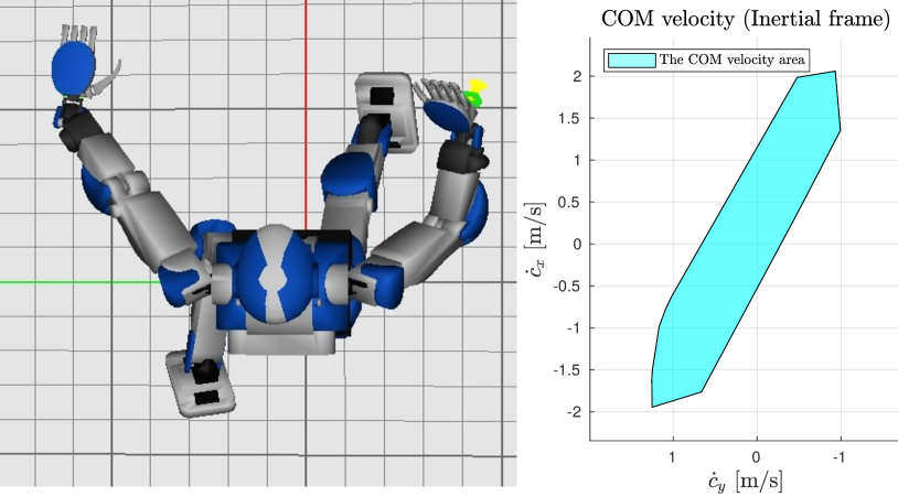
Figure 6: The cyan area represents the CoM velocity area $\mathcal{X}_{[{\dot{{\text{\bf c}}}}_{xy}]}$, obtained by iteratively solving (22-25) for the joint and contact configurations shown on the left (the same stance as in Fig. 5).

The inequalities (23) include the joint torque limits (13) and collect the CWC constraint (12) for the ${\text{m}_{\text{sc}}}$ sustained contacts. The equality (24) reformulates (17):

Similarly, the equality (25) reformulates (21):

$$\begin{bmatrix}{\dot{{\text{\bf c}}}}_{x}\\ {\dot{{\text{\bf c}}}}_{y}\end{bmatrix}=\underbrace{\frac{\text{w}(h-0pt{{\text{\bf c}}})}{\text{m}\cdot g}{\mathds{1}_{\boldsymbol{W},[:2,:]}}}_{E}\underbrace{\begin{bmatrix}\boldsymbol{W}_{1}\\ \vdots\\ \boldsymbol{W}_{{\text{m}_{\text{sc}}}}\end{bmatrix}}_{\boldsymbol{W}}+\underbrace{\text{w}{\text{\bf c}}}_{f},$$

where $h$ denotes the height of the projection plane, i.e., $h=0$; see Remark IV.1. As the resultant force corresponds to the first two rows of ${\boldsymbol{W}_{\text{O}}}$, ${\mathds{1}_{\boldsymbol{W},[:2,:]}}$ denotes the corresponding part of ${\mathds{1}_{\boldsymbol{W}}}$.

Remark IV.1

We are free to choose the height $h$ of the projection plane as long as $h\neq 0pt{{\text{\bf c}}}$. In this paper, we apply $h=0$, which is lower than the CoM height $0pt{{\text{\bf c}}}$. Hence, the inverted pendulum dynamics ${\dot{{\text{\bf c}}}}=-\text{w}({\text{\bf c}}-{\boldsymbol{\xi}})$ is appropriate. Otherwise, we need the pendulum dynamics: ${\dot{{\text{\bf c}}}}=\text{w}({\text{\bf c}}-{\boldsymbol{\xi}})$ due to the flipped sign of $h-0pt{{\text{\bf c}}}$; see the details in [3]. $\blacksquare$

V Solving the contact velocity

This section introduces the optimization problem for solving the optimal contact velocity. Sec. V-A predicts the set of post-impact CoM velocities $\mathcal{X}_{{{\dot{{\text{\bf c}}}}}^{+}_{xy}}$ according to the frictional impact mechanics in three dimensions, and Sec. V-B formulates the inequalities that can impose $\mathcal{X}_{{{\dot{{\text{\bf c}}}}}^{+}_{xy}}\subseteq\mathcal{X}_{[{\dot{{\text{\bf c}}}}_{xy}]}$ after the impact. Sec. V-C summarizes the detailed steps.

V-A The whole-body impact model

The recent analytical computation [41] of the set of candidate impulses $\mathcal{X}_{\boldsymbol{\iota}}$ base on the following assumptions:

1. The impact induces significant impulsive contact forces and negligible contact torques [19][42]. Recently, Gong and Grizzle [43] validated this assumption with the biped Cassie robot.

2. The impulse fulfills Coulomb’s friction law [15, 19].

3. The impacting end-effector has a tiny contact area compared to the robot dimensions such that a point contact model is appropriate [42].

4. The impact detection is timely such that the impacting end-effector can immediately pull back without exerting additional impulse.

5. The robot is kinematically controlled with high gains, enabling it to behave like a composite-rigid body (CRB) during an impact event. This assumption applies to robots that are actuated with electrical motors and high reduction-ratio gearboxes [11, 10].

The intersection between the friction cone and the planes of restitution (due to the uncertain restitution coefficient $c_{\text{r}}\in[\underline{c_{\text{r}}},\overline{c_{\text{r}}}]$) formulates the impulse set $\mathcal{X}_{\boldsymbol{\iota}}$ [41, Sec. 4.1].

According to assumption 5), during the impact event the robot behaves like a rigid body. Thus, the 6-dimensional velocity transform from the contact point frame $\mathcal{F}_{\boldsymbol{p}}$ to the CoM writes:

$${\color[rgb]{0.2578125,0.4921875,0.9609375}{\color[rgb]{0.2578125,0.4921875,0.9609375}Ad^{-1}_{g_{\boldsymbol{p}{\text{\bf c}}}}}}={\color[rgb]{0.2578125,0.4921875,0.9609375}\begin{bmatrix}R^{\top}_{\boldsymbol{p}{\text{\bf c}}}&-R^{\top}_{\boldsymbol{p}{\text{\bf c}}}\widehat{\boldsymbol{p}}_{\boldsymbol{p}{\text{\bf c}}}\\ 0&R^{\top}_{\boldsymbol{p}{\text{\bf c}}}\end{bmatrix}}.$$

According to assumption 1), the impact does not exert sudden change of momentum. Thus, we can compute the set of candidate CoM velocity jumps $\mathcal{X}_{\Delta{\dot{{\text{\bf c}}}}_{xy}}$ utilizing the upper-right corner of ${\color[rgb]{0.2578125,0.4921875,0.9609375}{\color[rgb]{0.2578125,0.4921875,0.9609375}Ad^{-1}_{g_{\boldsymbol{p}{\text{\bf c}}}}}}$ as:

$${\mathcal{X}_{\Delta{\dot{{\text{\bf c}}}}}\vcentcolon=\{\Delta{\dot{{\text{\bf c}}}}\in\mathbb{R}^{3}:\begin{bmatrix}\Delta{\dot{{\text{\bf c}}}}=\frac{1}{\text{m}}R_{{\text{\bf c}}\boldsymbol{p}}\boldsymbol{\iota},\\ \boldsymbol{\iota}\in\mathcal{X}_{\boldsymbol{\iota}}.\end{bmatrix}\},}$$ (26)

where $\text{m}\in\mathbb{R}^{+}$ denotes the robot mass, $R_{{\text{\bf c}}\boldsymbol{p}}$ denotes the rotation from CoM to the contact point, and the impulse set $\mathcal{X}_{\boldsymbol{\iota}}$ is taken from [41, Sec. 4.1].

Knowing the pre-impact CoM velocity ${\dot{{\text{\bf c}}}}^{-}_{xy}$, the set of post-impact planar CoM velocities are computed as:

$${\mathcal{X}_{{{\dot{{\text{\bf c}}}}}^{+}_{xy}}\vcentcolon=\{{{\dot{{\text{\bf c}}}}}^{+}_{xy}\in\mathbb{R}^{2}:\begin{bmatrix}{{\dot{{\text{\bf c}}}}}^{+}_{xy}={\dot{{\text{\bf c}}}}^{-}_{xy}+\Delta{\dot{{\text{\bf c}}}}_{xy}\\ \Delta{\dot{{\text{\bf c}}}}_{xy}\in\mathcal{X}_{\Delta{\dot{{\text{\bf c}}}}_{xy}}\end{bmatrix}\}.}$$ (27)

V-B The post-impact CoM velocity constraint

According to the phase-plane analysis [5, 6], as long as the post-impact CoM velocity ${{\dot{{\text{\bf c}}}}}^{+}_{xy}$ is within the CoM velocity area $\mathcal{X}_{[{\dot{{\text{\bf c}}}}_{xy}]}$:

$${{\dot{{\text{\bf c}}}}}^{+}_{xy}\in\mathcal{X}_{[{\dot{{\text{\bf c}}}}_{xy}]},$$

the robot can regulate CoM velocity to the origin by the sustained contact wrenches.

Since $\mathcal{X}_{{{\dot{{\text{\bf c}}}}}^{+}_{xy}}$ is a convex set, see Remark V.1, as long as each vertex of $\mathcal{X}_{{{\dot{{\text{\bf c}}}}}^{+}_{xy}}$ is within $\mathcal{X}_{[{\dot{{\text{\bf c}}}}_{xy}]}$, the entire set $\mathcal{X}_{{{\dot{{\text{\bf c}}}}}^{+}_{xy}}$ fulfills

$${\mathcal{X}_{{{\dot{{\text{\bf c}}}}}^{+}_{xy}}\subset\mathcal{X}_{[{\dot{{\text{\bf c}}}}_{xy}]}.}$$ (28)

In the following, we show how to impose the constraint (28) in an optimization problem.

Remark V.1

$\mathcal{X}_{{{\dot{{\text{\bf c}}}}}^{+}_{xy}}$ is convex due to: (1) the impulse set $\mathcal{X}_{\boldsymbol{\iota}}$ is convex by construction. (2) the affine operations, translations and rotations in (26) and (27) preserves convexity. $\blacksquare$

We discritize the Coulumb’s friction cone with $N_{\mu}$ vertices. The impulse set $\mathcal{X}_{\boldsymbol{\iota}}$ consists of the interior of the intersection between the two planes of restitution [41, Sec. 4.1.3] and the Coulumb’s friction cone, e.g., Fig. 7. Thus, $\mathcal{X}_{\boldsymbol{\iota}}$ has $2N_{\mu}$ vertices:

$${\begin{cases}\boldsymbol{\iota}_{2i}&={\text{K}_{(:,i)}}{\lambda_{2i}}\\ \boldsymbol{\iota}_{2i+1}&={\text{K}_{(:,i)}}{\lambda_{2i+1}}\\ \end{cases}\text{for}\leavevmode\nobreak\ i=0,\ldots,N_{\mu}-1,}$$ (29)

where ${\text{K}_{(:,i)}}\in\mathbb{R}^{3}$ denotes the $i$th column of the Coulumb’s friction cone ${\text{K}_{\mu}}\in\mathbb{R}^{3\times N_{\mu}}$, and ${\lambda_{2i}},{\lambda_{2i+1}}\in\mathbb{R}^{+}$ denote the positive scalars. The vertices $\boldsymbol{\iota}_{i}$ for $i=0,\ldots,2N_{\mu}-1$ also fulfill the planes of restitution:

$${\begin{aligned} \overline{c_{\text{r}}}{\boldsymbol{v}}^{+}_{z}&=-\boldsymbol{v}_{z}^{-}+{\widehat{\boldsymbol{\boldsymbol{z}}}}^{\top}W\boldsymbol{\iota}_{2i},\\ \underline{{c_{\text{r}}}}{\boldsymbol{v}}^{+}_{z}&=-\boldsymbol{v}_{z}^{-}+{\widehat{\boldsymbol{\boldsymbol{z}}}}^{\top}W\boldsymbol{\iota}_{2i+1},\end{aligned}\text{for }i=0,\ldots,N_{\mu}-1.}$$ (30)

where the inverse inertia $W\in\mathbb{R}^{3\times 3}$ denotes the impulse-to-velocity mapping and keeps constant as the robot configuration does not change during the impact event, $\boldsymbol{v}_{z}^{-}$ denotes the pre-impact contact velocity along the normal direction $\widehat{\boldsymbol{\boldsymbol{z}}}\in\mathbb{R}^{3,}$, and the uncertain restitution coefficient fulfills $c_{\text{r}}\in[\underline{c_{\text{r}}},\overline{c_{\text{r}}}]$.

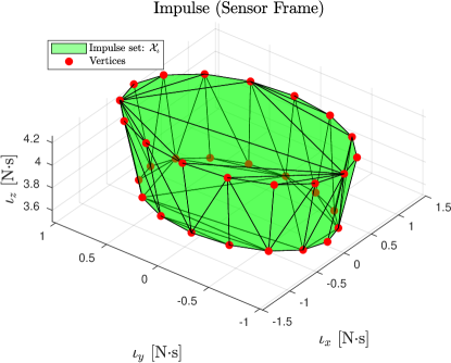
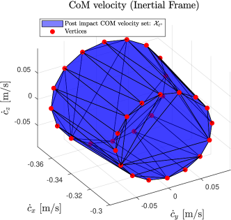
Figure 7: For the HRP-4 robot given in Fig. 5, we choose $N_{\mu}$ = 16 and visualize $2N_{\mu}$ vertices (red dots) of impulse set $\mathcal{X}_{\boldsymbol{\iota}}$ and the CoM velocity set $\mathcal{X}_{{\dot{{\text{\bf c}}}}}$. The friction coefficient at the impact surface is $0.24$, and the restitution coefficients are limited to $c_{\text{r}}\in[0,0.2]$.

Therefore, employing ${\lambda_{i}}$, for $i=0,\ldots,2(N_{\mu}-1)$ as optimization variables, the solver is aware of the set of post-impact impulses $\mathcal{X}_{\boldsymbol{\iota}}$ according to the impulse-set constraint:

$$\hbox{\pagecolor{gray!20}$\displaystyle\text{For }i=0,\ldots,N_{\mu}-1:$}$$ (31)

$$\hbox{\pagecolor{gray!20}$\displaystyle\text{Friction cone:}$}\begin{cases}{\boldsymbol{\lambda}_{2i}}&\geq\mathbf{0}\\ {\boldsymbol{\lambda}_{2i+1}}&\geq\mathbf{0},\end{cases}$$

$$\hbox{\pagecolor{gray!20}$\displaystyle\text{Plane of restitution: \eqref{eq:por}}$},$$

$$(\overline{c_{\text{r}}}+1)J_{3}\mathbf{\dot{q}}={\widehat{\boldsymbol{\boldsymbol{z}}}}^{\top}W{\text{K}_{(:,i)}}{\boldsymbol{\lambda}_{2i}},$$

$$(\underline{{c_{\text{r}}}}+1)J_{3}\mathbf{\dot{q}}={\widehat{\boldsymbol{\boldsymbol{z}}}}^{\top}W{\text{K}_{(:,i)}}{\boldsymbol{\lambda}_{2i+1}},$$

where $J_{3}\mathbf{\dot{q}}$ computes the contact velocity along the normal direction.

We denote the $2i$-th vertex of $\mathcal{X}_{{{\dot{{\text{\bf c}}}}}^{+}_{xy}}$ as $\mathcal{X}_{{{\dot{{\text{\bf c}}}}}^{+}_{xy},2i}\in\mathbb{R}^{2}$. Given the mappings (26), (27), and the impulse vertices $\boldsymbol{\iota}_{2i},\boldsymbol{\iota}_{2i+1}$ defined by (29) and (30), $\mathcal{X}_{{{\dot{{\text{\bf c}}}}}^{+}_{xy},2i}$ writes:

$$\mathcal{X}_{{{\dot{{\text{\bf c}}}}}^{+}_{xy},2i} =\dot{{\text{\bf c}}}_{x,y}^{-}+\frac{1}{\text{m}}\begin{bmatrix}1,&0,&0\\ 0,&1,&0\end{bmatrix}R_{{\text{\bf c}}\boldsymbol{p}}{\text{K}_{(:,i)}}{\boldsymbol{\lambda}_{2i}},$$

$$\mathcal{X}_{{{\dot{{\text{\bf c}}}}}^{+}_{xy},2i+1} =\dot{{\text{\bf c}}}_{x,y}^{-}+\frac{1}{\text{m}}\begin{bmatrix}1,&0,&0\\ 0,&1,&0\end{bmatrix}R_{{\text{\bf c}}\boldsymbol{p}}{\text{K}_{(:,i)}}{\boldsymbol{\lambda}_{2i+1}}.$$

Therefore, we reformulate (28) as the following post-impact CoM velocity constraint for $i=0,\ldots,N_{\mu}-1$:

$${\begin{aligned} &\underbrace{\dot{{\text{\bf c}}}_{x,y}^{-}+\frac{1}{\text{m}}\begin{bmatrix}1,&0,&0\\ 0,&1,&0\end{bmatrix}R_{{\text{\bf c}}\boldsymbol{p}}{\text{K}_{(:,i)}}{\boldsymbol{\lambda}_{2i}}}_{\mathcal{X}_{{{\dot{{\text{\bf c}}}}}^{+}_{xy},2i}}\in\mathcal{X}_{[{\dot{{\text{\bf c}}}}_{xy}]};\\ &\underbrace{\dot{{\text{\bf c}}}_{x,y}^{-}+\frac{1}{\text{m}}\begin{bmatrix}1,&0,&0\\ 0,&1,&0\end{bmatrix}R_{{\text{\bf c}}\boldsymbol{p}}{\text{K}_{(:,i)}}{\boldsymbol{\lambda}_{2i+1}}}_{\mathcal{X}_{{{\dot{{\text{\bf c}}}}}^{+}_{xy},2i+1}}\in\mathcal{X}_{[{\dot{{\text{\bf c}}}}_{xy}]},\\ \end{aligned},}$$ (32)

which modifies the solver’s search space to impose the balance condition (28). We assume $\mathcal{X}_{[{\dot{{\text{\bf c}}}}_{xy}]}$ has $n_{c}$ vertices. In order to implement $\mathcal{X}_{{{\dot{{\text{\bf c}}}}}^{+}_{xy},i}\in\mathcal{X}_{[{\dot{{\text{\bf c}}}}_{xy}]}$, we have to re-write the vertex-represented $\mathcal{X}_{[{\dot{{\text{\bf c}}}}_{xy}]}$ as the half-space representation $[G_{\mathcal{X}_{[{\dot{{\text{\bf c}}}}_{xy}]}}\in\mathbb{R}^{n_{c}\times 2},h_{\mathcal{X}_{[{\dot{{\text{\bf c}}}}_{xy}]}}\in\mathbb{R}^{n_{c}}]$, and reformulate (32) as:

$${\begin{aligned} G_{\mathcal{X}_{[{\dot{{\text{\bf c}}}}_{xy}]}}\mathcal{X}_{{{\dot{{\text{\bf c}}}}}^{+}_{xy},i}\leq h_{\mathcal{X}_{[{\dot{{\text{\bf c}}}}_{xy}]}},\end{aligned}\quad\text{for}\quad i=1,\ldots,2N_{\mu}-1.}$$ (33)

There are standard approaches to convert between vertex representation and the half-space representation of a polytope, e.g., the double description method [44].

V-C Quadratic program formulation

As a minimalistic example, we can formulate an optimization problem which takes the following form:

$$\min_{\mathbf{\dot{q}},{\boldsymbol{\lambda}_{\mu}}} {{\left\lVert J\mathbf{\dot{q}}-\boldsymbol{v}^{\text{ref}}\right\rVert}^{2}}$$ (34)

s.t. $$\hbox{\pagecolor{blue!20}$\displaystyle\text{The impulse-set constraint \eqref{eq:impulse-set-constraints}},$}$$

$$\hbox{\pagecolor{blue!20}$\displaystyle\text{The post-impact CoM velocity constraint \eqref{eq:picomd-constraint}},$}$$

$$\text{Other impact-aware constraints, see Remark\leavevmode\nobreak\ \ref{remark:impulse-torque}}.$$

where the high-lighted constraints are mandatory to meet the proposed balance criteria. See the detailed formulation steps in Algorithm 1.

By solving (34), we can obtain the maximum feasible contact velocity $J{\mathbf{\dot{q}}}^{*}$ for a whole-body controller [36, 45, 46]. As an example, formulating and solving (34) leads to the contact velocity $J{\mathbf{\dot{q}}}^{*}=0.397$ m/s for the HRP-4 stance in Fig. 5. Applying this velocity would result in a vertex of the set $\mathcal{X}_{{{\dot{{\text{\bf c}}}}}^{+}_{xy}}$ (visualized in Fig. 7) overlapping with the boundary of $\mathcal{X}_{[{\dot{{\text{\bf c}}}}_{xy}]}$ in Fig. 8, thereby satisfying the condition (28).

To illustrate the solution’s optimality, we additionally plotted the sets $\mathcal{X}_{{{\dot{{\text{\bf c}}}}}^{+}_{xy}}$ resulted from a series of increasing contact velocities $0.0794,0.159,0.238,0.318$ m/s in Fig. 8, assuming that the background colored areas are the actual CoM velocity area $\mathcal{X}_{[{\dot{{\text{\bf c}}}}_{xy}]}$. Hence, the optimizer would increase the contact velocity to $0.397$ m/s.

The geometric size of the set $\mathcal{X}_{{{\dot{{\text{\bf c}}}}}^{+}_{xy}}$ varies with respect to the friction coefficient at the impact surface. We show different optimal contact velocities $J{\mathbf{\dot{q}}}^{*}$ resulting from the variation in friction coefficient Fig. 9.

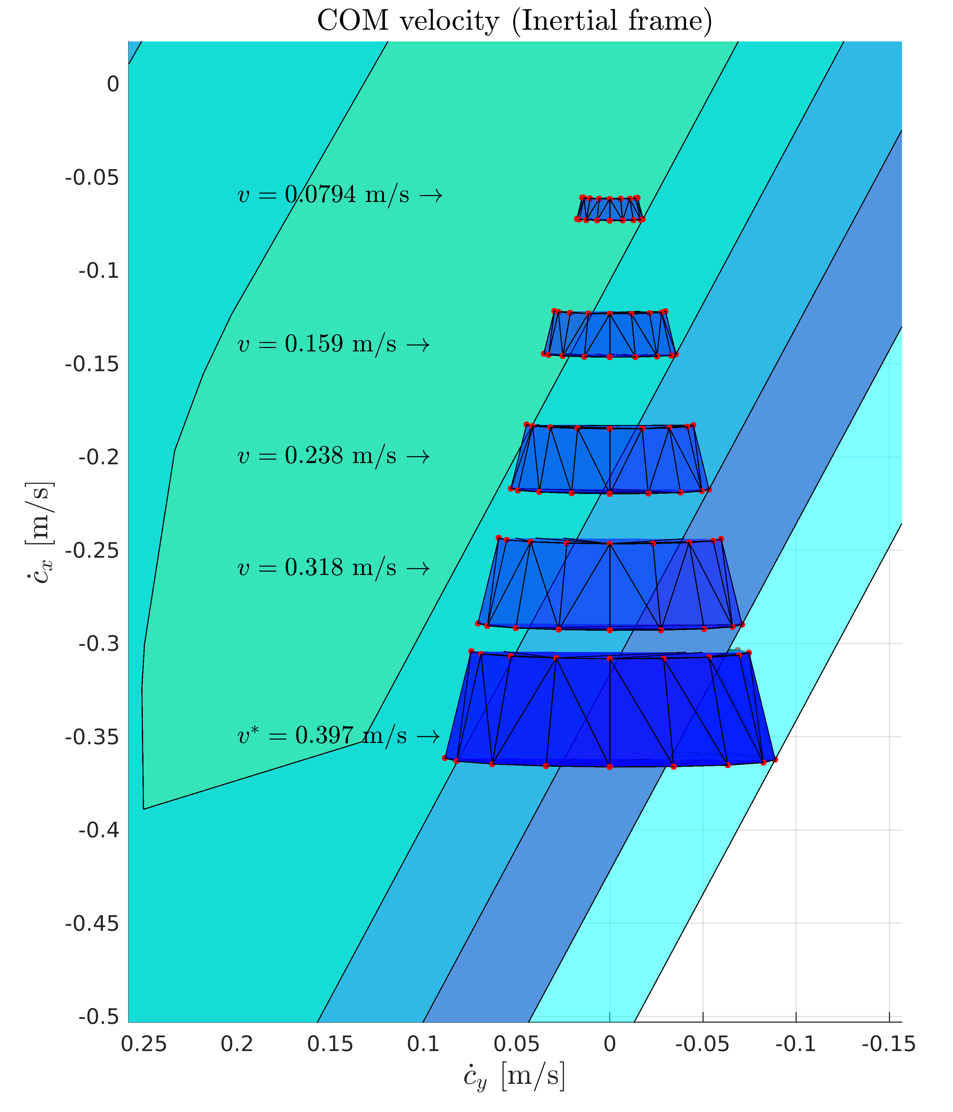
Figure 8: Illustration of the relation between contact velocity $J\mathbf{\dot{q}}$ and the corresponding post-impact CoM velocity set $\mathcal{X}_{{{\dot{{\text{\bf c}}}}}^{+}_{xy}}$. As $J\mathbf{\dot{q}}$ increases, the solver identified the maximum contact velocity $J\mathbf{\dot{q}}=0.397$ m/s without violating the condition $\mathcal{X}_{{{\dot{{\text{\bf c}}}}}^{+}_{xy}}\subset\mathcal{X}_{[{\dot{{\text{\bf c}}}}_{xy}]}$. The different colored areas indicate corresponding hypothetical CoM velocity areas that would be defined, if the contact velocities $0.0794,0.159,0.238,0.318$ m/s were found to be optimal.

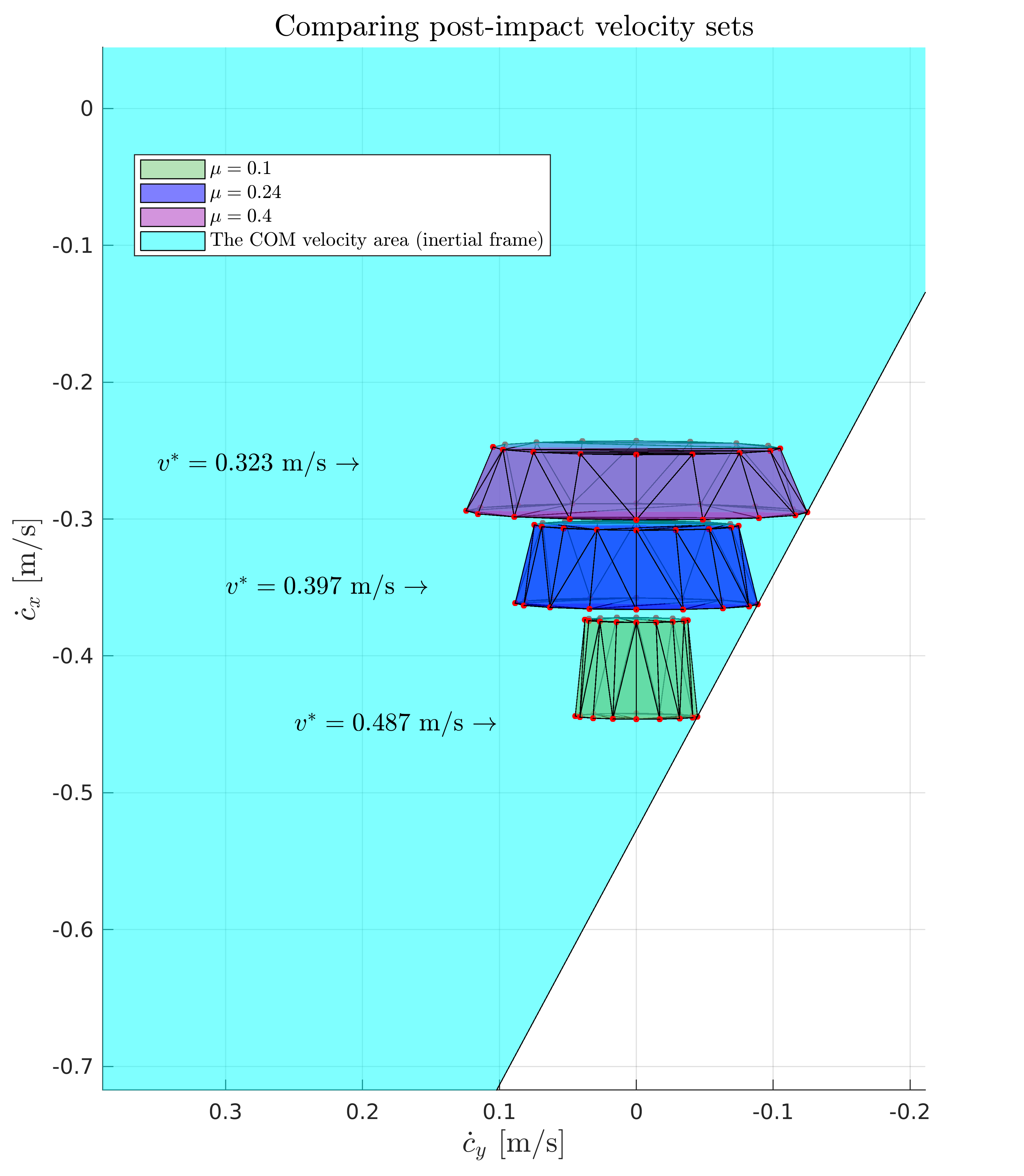
Figure 9: This figure compares the optimal solutions for friction coefficients of $0.1$, $0.24$, and $0.4$. As the geometric size of the post-impact CoM velocity set $\mathcal{X}_{{{\dot{{\text{\bf c}}}}}^{+}_{xy}}$ varies with the friction coefficient, the solver identifies different optimal contact velocities.

Remark V.2

To protect the hardware resilience bounds, we can additionally apply the impact-aware constraints for $i=0,\ldots,N_{\mu}-1$:

$$\begin{aligned} &\hbox{\pagecolor{gray!20}$\displaystyle\text{Post-impact joint velocity: \cite[cite]{[\@@bibref{}{wang2020ijrr}{}{}, eq.\leavevmode\nobreak\ 29]}}$},\\ &\underline{\mathbf{\dot{q}}}\leq\mathbf{\dot{q}}^{-}+{J}^{\top}{(J{J}^{\top})}^{-1}W{\text{K}_{(:,i)}}{\boldsymbol{\lambda}_{2i}}\leq\overline{\mathbf{\dot{q}}},\\ &\underline{\mathbf{\dot{q}}}\leq\mathbf{\dot{q}}^{-}+{J}^{\top}{(J{J}^{\top})}^{-1}W{\text{K}_{(:,i)}}{\boldsymbol{\lambda}_{2i+1}}\leq\overline{\mathbf{\dot{q}}},\\ &\hbox{\pagecolor{gray!20}$\displaystyle\text{Post-impact joint torque: \cite[cite]{[\@@bibref{}{wang2020ijrr}{}{}, eq.\leavevmode\nobreak\ 30]}}$},\\ &\underline{\boldsymbol{\tau}}\leq\boldsymbol{\tau}^{-}+\frac{a}{\delta t}{J}^{\top}{\text{K}_{(:,i)}}{\boldsymbol{\lambda}_{2i}}\leq\overline{\boldsymbol{\tau}},\\ &\underline{\boldsymbol{\tau}}\leq\boldsymbol{\tau}^{-}+\frac{a}{\delta t}{J}^{\top}{\text{K}_{(:,i)}}{\boldsymbol{\lambda}_{2i+1}}\leq\overline{\boldsymbol{\tau}}\\ \end{aligned},$$ (35)

where the impact duration $\delta t$ and the positive scalar $a$ facilitate the prediction of impulsive torque [41, Sec. 4.3]. $\blacksquare$

Algorithm 1 Solve the maximum balance-constraint-aware contact velocity $J{\mathbf{\dot{q}}}^{*}$

Inputs: (1) The robot’s joint positions $\mathbf{q}$, velocities $\mathbf{\dot{q}}$; (2) The contact configurations, i.e., the contact area’s geometric size and friction coefficients, for computing the contact wrench cone (12); (3) The impact end-effector’s friction coefficient; (4) The reference contact velocity $\boldsymbol{v}^{\text{ref}}\in\mathbb{R}^{3}$.
Outputs: The maximum contact velocity $J{\mathbf{\dot{q}}}^{*}$ without leading to a fall.

1:procedure Initialization (High-dimensional represented $\mathcal{X}_{[{\dot{{\text{\bf c}}}}_{xy}]}$)

2:     Contact wrench cones (12).

3:     Limited actuation torques (13).

4:     LIPM assumptions (17).

5:     CoM velocity dependence on ZMP (21).

6:end procedure

7:procedure Projection

8:     Iteravtively solving (22-25) to obtain vertices of the two-dimensional $\mathcal{X}_{[{\dot{{\text{\bf c}}}}_{xy}]}$, [8, 47].

9:end procedure

10:procedure Solve and execute $J{\mathbf{\dot{q}}}^{*}$

11:     Solve QP (34) with impulse set (31) and post-impact CoM velocity (33) constraints for $J{\mathbf{\dot{q}}}^{*}$

12:     Track $J{\mathbf{\dot{q}}}^{*}$ and fulfill other task-space objectives using a whole-body QP, such as [36, 46].

13:end procedure

VI Validation

Employing the full-size humanoid robot HRP-4 with 34 actuated joints, we validate the proposed approach through the following experiments and simulations:

1. [Experiment: Impacting a Location-Unknown Wall] To show that the CoM velocity is a less-conservative measure than ZMP, we strictly restrict the ZMP with the support polygon ${\text{\bf z}}\in\mathcal{X}_{\mathcal{S}}$ following the impact-aware QP formulation [41] and found a contact velocity of $0.11$ m/s. In another trial, we tried a significantly higher contact velocity $0.345$ m/s. Despite the violation of the ZMP criteria ${\text{\bf z}}\in\mathcal{X}_{\mathcal{S}}$, the robot maintained its balance and did not fall.

2. [Experiment: Push Recovery with Two Non-coplanar Contacts] To validate the proposed CoM velocity area $\mathcal{X}_{[{\dot{{\text{\bf c}}}}_{xy}]}$ in Sec. IV, we placed the HRP-4 robot on two non-coplanar contacts. Pushing the robot from different directions, we observed that the ZMP momentarily jumped outside the multi-contact support area [3], while the robot did not fall. Throughout the experiment, the proposed CoM velocity area condition ${{\dot{{\text{\bf c}}}}}^{+}_{xy}\in\mathcal{X}_{[{\dot{{\text{\bf c}}}}_{xy}]}$ was always respected.

1. [Simulation: Maximum Contact Velocities for various stances] We determined the maximum contact velocity by solving problem (34) for three different scenarios: (1) pushing with two coplanar contacts as shown in Fig. 1; (2) pushing with two non-coplanar contacts; (3) kicking with one foot contact.

VI-A Experiment 1 Impacting a Location-Unknown Wall

Experiment setup

The HRP-4 Robot’s joints are controlled in position at $1000$ Hz, while the mid-level QP controller [45] samples the ATI-45 force-torque sensors mounted on the ankles and palms at $200$ Hz. The friction coefficient for the feet contacts is set to $0.7$, and the robot does not have prior knowledge of the position of the concrete wall shown in Fig. 10.

Optimization-based whole-body controllers rely on closed-form calculations to formulate the optimization problem during each sampling period. The analytical impact model [4] can only predict sudden changes of momentum or impulse $\boldsymbol{\iota}$. In order to predict the sudden change of the ZMP, we artificially set the impact duration $\delta t=5$ ms to predict the impulsive force as $\Delta\boldsymbol{f}=\frac{\boldsymbol{\iota}}{\delta t}$.

ZMP-based criteria validation

Our QP controller commanded the HRP-4’s right palm to hit a wall with exceptionally-high reference contact velocity $0.8$ m/s, see Fig. 10. We mounted a 3D printed plastic palm with $3$ cm thickness.

Employing the predicted $\Delta\boldsymbol{f}$, the optimization solver reduced the contact velocity to 0.11 m/s, see Fig. 12 to ensure the balance criterion ${\text{\bf z}}\in\mathcal{X}_{\mathcal{S}}$. The robot immediately pulled back the right palm as soon as the force-torque measurements reached 15 N.

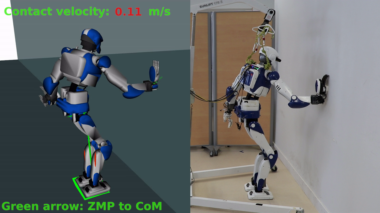
Figure 10: The snap shot of the HRP-4 robot hitting the wall at $0.11$ m/s while strictly fulfilling ${\text{\bf z}}\in\mathcal{X}_{\mathcal{S}}$ https://youtu.be/TL34EWORwbU. The green arrow connects the CoM and the ZMP on the ground. The red arrows indicate the ground reaction forces.

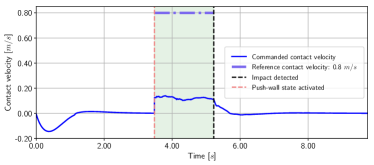
Figure 11: In order to meet the ZMP-based balance criterion ${\text{\bf z}}\in\mathcal{X}_{\mathcal{S}}$, the impact-aware QP [41] reduced the contact velocity to $0.11$ m/s from a high reference $0.8$ m/s.

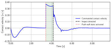
Figure 12: Without considering the ZMP-based balance criterion ${\text{\bf z}}\in\mathcal{X}_{\mathcal{S}}$, we increased the contact velocity to $0.34$ m/s. The robot did not fall as robot regulated the CoM velocity to the origin in the right corner of Fig. 1.

We observed that the right plam’s impact was considerably gentle. Thus, in another trial, we removed the constraint ${\text{\bf z}}\in\mathcal{X}_{\mathcal{S}}$ and changed the contact velocity reference to $0.34$ m/s. Despite the ZMP jumped outside the support polygon, see Fig. 1, the robot did not fall, see the analysis in Sec. III-B.

Fulfilling zero-step capture region

In contrast, according to the CoM velocity, the robot will not fall after the impact at $0.34$ m/s because the CoM velocities strictly lie within the zero-step capture region, as shown in Fig. 1.

VI-B Experiment 2 Push recovery on two non-coplanar contacts

Experiment setup

We placed the HRP-4 robot on two non-coplanar contacts, see Fig. 13 and regulated the CoM dynamics with the LIPM stabilizer through the mc$\_$rtc framework.

The state-of-the-art balance criteria [3] for non-copalnar contacts requires ZMP to stay strictly within the ZMP support area ${\mathcal{X}_{[{\text{\bf z}}]}}$, e.g., the light blue region in Fig. 14 (or the red polygon in Fig. 13), which is the extension of the support polygon for coplanar contacts.

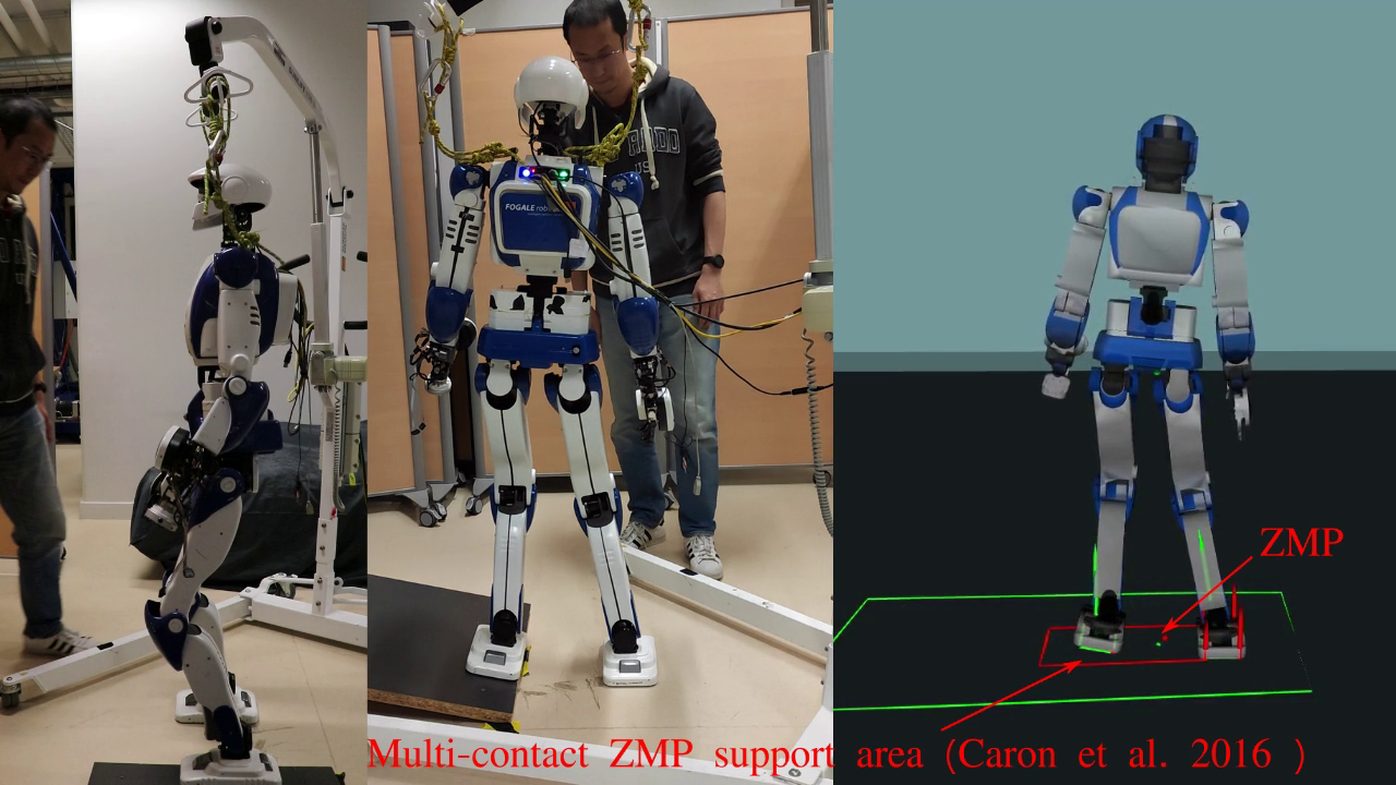
Figure 13: From left to right, we show the side, back and simulation view of the HRP-4 robot on two non-coplanar contacts. The red dot and the red rectangle correspond to ZMP z and the ZMP support area ${\mathcal{X}_{[{\text{\bf z}}]}}$ by [3]. The green dot and the green rectangle correspond to the CoM velocity ${\dot{{\text{\bf c}}}}_{xy}$ and the proposed CoM velocity area $\mathcal{X}_{[{\dot{{\text{\bf c}}}}_{xy}]}$.

Balance criteria comparison

The operator pushed the HRP-4 robot from front, side, and back, respectively and for multiple times. The ZMP temporarily violated the ZMP support area ${\mathcal{X}_{[{\text{\bf z}}]}}$ for several times without leading to a fall, see Fig. 14. On the other hand, during the same experiment the CoM velocity ${\dot{{\text{\bf c}}}}_{xy}$ strictly fulfilled the CoM velocity area $\mathcal{X}_{[{\dot{{\text{\bf c}}}}_{xy}]}$, see Fig. 15. Thus, we conclude that the condition ${{\dot{{\text{\bf c}}}}}^{+}_{xy}\in\mathcal{X}_{[{\dot{{\text{\bf c}}}}_{xy}]}$ is more accurate than state-of-the-art ZMP-based balance criteria.

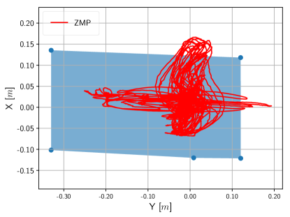
Figure 14: The ZMP trajectory (red line) and the ZMP support area ${\mathcal{X}_{[{\text{\bf z}}]}}$ (grey rectangle) during the push-recovery experiment. Temporary violations of the ZMP support area, indicated by z values outside of ${\mathcal{X}_{[{\text{\bf z}}]}}$, did not result in a fall.

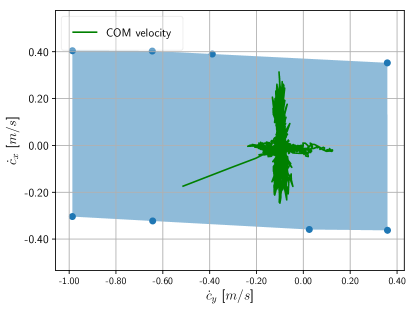
Figure 15: Trajectory of the CoM velocity ${\dot{{\text{\bf c}}}}_{xy}$ plotted against the CoM velocity area $X[\dot{x}_{c}]$, during the push-recovery experiment. The spike pointing in the down-left direction corresponds to the initial motion, when the robot established non-coplanar contact on the ramp.

VI-C Simulation 1 On-purpose impact for various stances

In order to evaluate the maximum contact velocities for various on-purpose impact tasks, we follow the steps outlined in Algorithm 1 to formulate and solve (34) for the maximum contact velocity $J{\mathbf{\dot{q}}}^{*}$ which is the highest contact velocity without breaking (28).

As elaborated in Sec. V-C and visualized in Fig. 6, applying $J{\mathbf{\dot{q}}}^{*}$ would enable the boundaries of the post-impact CoM velocities $\mathcal{X}_{{{\dot{{\text{\bf c}}}}}^{+}_{xy}}$ and the CoM velocity area $\mathcal{X}_{[{\dot{{\text{\bf c}}}}_{xy}]}$ overlap with each other. We will refer to phenomenon as the overlapping condition in future discussions.

Additional details are available in the attached video, where we tuned the joint and contact configurations using a Graphical User Interface and visualize the CoM velocity area $\mathcal{X}_{[{\dot{{\text{\bf c}}}}_{xy}]}$.

Balance with two non-coplanar contacts

The two non-coplanar foot contacts with a friction coefficient $\mu=0.7$ in Fig. 16 lead to a significantly larger COM velocity area in Fig. 18 compared to Fig. 15.

To evaluate the maximum contact velocity, we kept the right palm as the impact end-effector with the same friction coefficient $\mu=0.2$ and restitution coefficient $c_{\text{r}}\in[0,0.2]$. Solving the QP (34) generated a higher contact velocity of $0.529$  m/s, which corresponds to the overlapping condition illustrated in Fig. 18 and the sets $\mathcal{X}_{\boldsymbol{\iota}}$ and $\mathcal{X}_{{{\dot{{\text{\bf c}}}}}^{+}_{xy}}$ in Fig. 17.

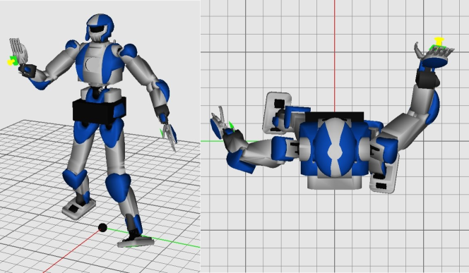
Figure 16: The HRP-4 robot balance with another two co-planar contacts.

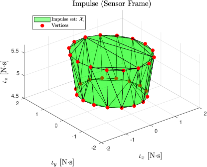
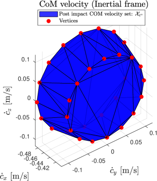
Figure 17: For the HRP-4 robot given in Fig. 1, we visualize vertices (red dots) of impulse set $\mathcal{X}_{\boldsymbol{\iota}}$ and the COM velocity set $\mathcal{X}_{{\dot{{\text{\bf c}}}}}$ when the contact velocity $J{\mathbf{\dot{q}}}^{*}=0.529$ m/s. The friction coefficient at the impact surface is $0.2$, and the restitution coefficients are limited to $c_{\text{r}}\in[0,0.2]$.

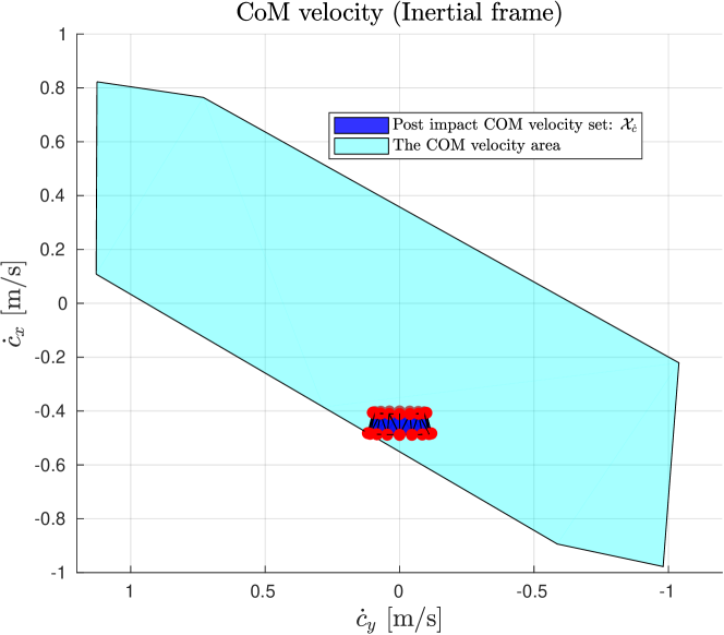
Figure 18: When the contact velocity in Fig. 16 reached $J{\mathbf{\dot{q}}}^{*}=0.529$ m/s, a vertex of the set $\mathcal{X}_{{\dot{{\text{\bf c}}}}}$ reaches the boundaries of $\mathcal{X}_{[{\dot{{\text{\bf c}}}}_{xy}]}$.

Kicking

Employing the right foot contact with friction coefficient $\mu=0.7$, the HRP-4 robot kicks with the left foot’s toe, see Fig. 19. We set the friction coefficient at the impact point as $\mu=0.24$ and restitution coefficient $c_{\text{r}}\in[0,0.2]$. The impact-aware QP (34) found the maximum contact velocity at $0.569$ m/s, which resulted in the sets $\mathcal{X}_{\boldsymbol{\iota}}$ and $\mathcal{X}_{{{\dot{{\text{\bf c}}}}}^{+}_{xy}}$ depicted in Fig. 20, and satisfied the overlapping condition in Fig. 19.

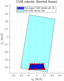
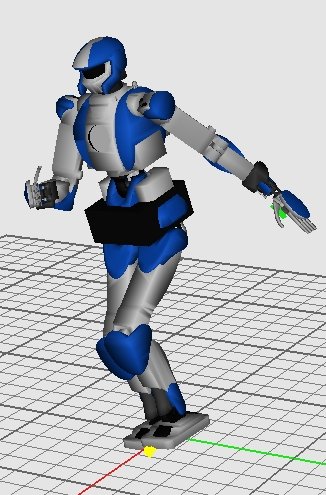
Figure 19: When the left toe kick at $J{\mathbf{\dot{q}}}^{*}=0.569$ m/s, a vertex of the set $\mathcal{X}_{{\dot{{\text{\bf c}}}}}$ hits the boundaries of $\mathcal{X}_{[{\dot{{\text{\bf c}}}}_{xy}]}$.

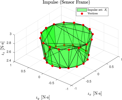
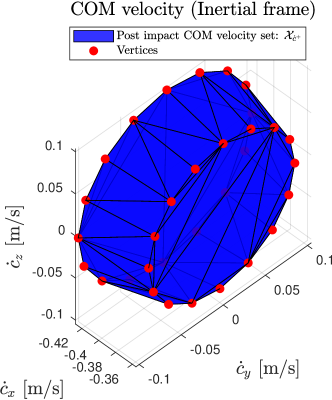
Figure 20: When the HRP-4 robot shown in Fig. 19 kicks at$J{\mathbf{\dot{q}}}^{*}=0.569$ m/s, we visualize vertices (red dots) of impulse set $\mathcal{X}_{\boldsymbol{\iota}}$ and the COM velocity set $\mathcal{X}_{{\dot{{\text{\bf c}}}}}$. The friction coefficient at the impact surface is $0.24$, and the restitution coefficients are limited to $c_{\text{r}}\in[0,0.2]$.

VII Conclusion

In order to deploy humanoid robots in a contact-rich environment, the balance criteria has to handle uneven ground and on-purpose impact tasks. Our observations of the full-size humanoid robot HRP-4 indicated that the state-of-the-art ZMP-based balance criteria is overly conservative and ill-defined in impulse dynamics.

To address this problem, we propose a CoM-velocity-based balance criteria for humanoid robots on non-coplanar contacts, and an optimization-based formulation that can solve for the maximum contact velocity while fulfilling the criteria. Our assumptions include (1) the contacts are rigid, (2) the robot is kinematic-controlled, (3) the robot can timely detect the collision such that the impact will be instantaneous without exerting additional momentum exchange, and (4) the sustained contacts do not break during the instantaneous impact event.

We validated our balance criteria through a push-recovery experiment on the HRP-4 robot, which sustained one foot on the ground and the other on a 30-degree ramp. To the best of our knowledge, this is the first successful push-recovery experiment for kinematic-controlled humanoid robot on non-coplanar contacts. Additionally, we evaluated the maximum contact velocities for other stances through simulations.

Our approach has significant potential in enabling humanoid robots to perform various impact tasks with greater standing stability in contact-rich environments. By determining the maximum foot contact velocities for different stances, we can plan and execute dynamic reference trajectories without breaking balance through impacts.

We acknowledge that the experimental validation of our approach is limited by the fragility of the HRP-4 robot, which has a payload of only $500$ grams. In future work, we will validate our approach on more robust platforms. Furthermore, we aim to investigate damping post-impact oscillations through compliant control modes.

-A Resultant torque

The wrench ${\boldsymbol{W}_{\text{O}}}=[{\boldsymbol{f}_{\text{O}}}^{\top},{\boldsymbol{\tau}_{\text{O}}}^{\top}]^{\top}$ at the origin $\boldsymbol{q}_{\text{O}}$ of the inertial frame will lead to torque at another point $\boldsymbol{q}_{x}$ as:

$${\boldsymbol{\tau}_{\boldsymbol{q}_{x}}={\boldsymbol{\tau}_{\text{O}}}+\overrightarrow{\boldsymbol{q}_{x}\boldsymbol{q}_{\text{O}}}\times{\boldsymbol{f}_{\text{O}}}={\boldsymbol{\tau}_{\text{O}}}+(\boldsymbol{q}_{\text{O}}-\boldsymbol{q}_{x})\times{\boldsymbol{f}_{\text{O}}}.}$$ (36)

-B Derivation of ZMP

According to ZMP definition, the resultant torque at ZMP $\boldsymbol{\tau}_{{\text{\bf z}}}$ is parallel to the ground surface normal n. Hence, we can derive the ZMP by substituting $\boldsymbol{\tau}_{{\text{\bf z}}}$ according to (36) into $\text{\bf n}\times\boldsymbol{\tau}_{{\text{\bf z}}}=0$:

$$\text{\bf n}\times\boldsymbol{\tau}_{{\text{\bf z}}} =\text{\bf n}\times({\boldsymbol{\tau}_{\text{O}}}+(\boldsymbol{q}_{\text{O}}-{\text{\bf z}})\times{\boldsymbol{f}_{\text{O}}})=0$$ (37)

$$\boldsymbol{q}_{\text{O}}=0\Rightarrow =\text{\bf n}\times{\boldsymbol{\tau}_{\text{O}}}-\text{\bf n}\times({\text{\bf z}}\times{\boldsymbol{f}_{\text{O}}})=0$$

$$=\text{\bf n}\times{\boldsymbol{\tau}_{\text{O}}}-({\text{\bf n}}^{\top}{\boldsymbol{f}_{\text{O}}}){\text{\bf z}}+({\text{\bf n}}^{\top}{\text{\bf z}}){\boldsymbol{f}_{\text{O}}}=0$$

$$\Rightarrow{\text{\bf z}} \vcentcolon=\frac{\text{\bf n}\times{\boldsymbol{\tau}_{\text{O}}}}{{\text{\bf n}}^{\top}{\boldsymbol{f}_{\text{O}}}}+\frac{({\text{\bf n}}^{\top}{\text{\bf z}}){\boldsymbol{f}_{\text{O}}}}{{\text{\bf n}}^{\top}{\boldsymbol{f}_{\text{O}}}}$$

$$=\frac{\text{\bf n}\times{\boldsymbol{\tau}_{\text{O}}}}{{\text{\bf n}}^{\top}{\boldsymbol{f}_{\text{O}}}}+0pt{{\text{\bf z}}}\frac{{\boldsymbol{f}_{\text{O}}}}{{\text{\bf n}}^{\top}{\boldsymbol{f}_{\text{O}}}}.$$

-C Contact wrench

The Newton-Euler equations of the robot writes:

$$\begin{bmatrix}\dot{P}\\ \dot{\mathcal{L}}\end{bmatrix}=\begin{bmatrix}\text{m}\ddot{{\text{\bf c}}}\\ \dot{\mathcal{L}}\end{bmatrix}=\begin{bmatrix}\text{m}\boldsymbol{g}\\ 0\end{bmatrix}+\sum^{{\text{m}_{\text{sc}}}}_{i=1}{\begin{bmatrix}\boldsymbol{f}_{i}\\ \overrightarrow{{\text{\bf c}}\boldsymbol{p}_{i}}\times\boldsymbol{f}_{i}\end{bmatrix}},$$ (38)

where $m$ denotes the total mass of the robot. The vector $\overrightarrow{{\text{\bf c}}\boldsymbol{p}_{i}}=\boldsymbol{\boldsymbol{p}_{i}}-\boldsymbol{{\text{\bf c}}}$ connects a contact point $\boldsymbol{p}_{i}$ to the CoM. Thus, $\boldsymbol{f}_{i}$ induces the torque $\overrightarrow{{\text{\bf c}}\boldsymbol{p}_{i}}\times\boldsymbol{f}_{i}$ at the CoM.

According to definition (1), the ${\text{m}_{\text{sc}}}$ sustained contact forces result in the wrench ${\boldsymbol{W}_{\text{O}}}$ at the inertial frame’s origin $\boldsymbol{q}_{\text{O}}$:

$${\boldsymbol{W}_{\text{O}}}=\begin{bmatrix}{\boldsymbol{f}_{\text{O}}}\\ {\boldsymbol{\tau}_{\text{O}}}\end{bmatrix}=\sum^{{\text{m}_{\text{sc}}}}_{i=1}{\begin{bmatrix}\boldsymbol{f}_{i}\\ \overrightarrow{\boldsymbol{q}_{\text{O}}\boldsymbol{p}_{i}}\times\boldsymbol{f}_{i}\end{bmatrix}}=\sum^{{\text{m}_{\text{sc}}}}_{i=1}{\begin{bmatrix}\boldsymbol{f}_{i}\\ \boldsymbol{p}_{i}\times\boldsymbol{f}_{i}\end{bmatrix}}.$$ (39)

According to the equations of motion (38), the resultant force is equal to:

$${\boldsymbol{f}_{\text{O}}}=\dot{P}-\text{m}\boldsymbol{g},$$

and we can expand $\dot{\mathcal{L}}$ as:

$$\dot{\mathcal{L}} =\sum^{{\text{m}_{\text{sc}}}}_{i=1}{\overrightarrow{{\text{\bf c}}\boldsymbol{p}_{i}}\times\boldsymbol{f}_{i}}=\sum^{{\text{m}_{\text{sc}}}}_{i=1}{(\boldsymbol{\boldsymbol{p}_{i}}-\boldsymbol{{\text{\bf c}}})\times\boldsymbol{f}_{i}}$$ (40)

$$=\underbrace{\sum^{{\text{m}_{\text{sc}}}}_{i=1}{\boldsymbol{p}_{i}\times\boldsymbol{f}_{i}}}_{{\boldsymbol{\tau}_{\text{O}}}}-{\text{\bf c}}\times\underbrace{\sum^{{\text{m}_{\text{sc}}}}_{i=1}{\boldsymbol{f}_{i}}}_{{\boldsymbol{f}_{\text{O}}}}$$

$$={\boldsymbol{\tau}_{\text{O}}}-{\text{\bf c}}\times{\boldsymbol{f}_{\text{O}}}.$$

-D Derivation of the whole-body dynamics (5)

By substituting ${\boldsymbol{f}_{\text{O}}}=\dot{P}-\text{m}\boldsymbol{g}$ and ${\boldsymbol{\tau}_{\text{O}}}=\dot{\mathcal{L}}+{\text{\bf c}}\times{\boldsymbol{f}_{\text{O}}}$ according to (40), we can re-write the ZMP definition (3):

$$({\text{\bf n}}^{\top}{\boldsymbol{f}_{\text{O}}}){\text{\bf z}} =\text{\bf n}\times{\boldsymbol{\tau}_{\text{O}}}+({\text{\bf n}}^{\top}{\text{\bf z}}){\boldsymbol{f}_{\text{O}}}$$

$$=\text{\bf n}\times(\dot{\mathcal{L}}+{\text{\bf c}}\times{\boldsymbol{f}_{\text{O}}})+({\text{\bf n}}^{\top}{\text{\bf z}}){\boldsymbol{f}_{\text{O}}}$$

$$=\text{\bf n}\times\dot{\mathcal{L}}+\text{\bf n}\times({\text{\bf c}}\times{\boldsymbol{f}_{\text{O}}})+({\text{\bf n}}^{\top}{\text{\bf z}}){\boldsymbol{f}_{\text{O}}}$$

$$=\text{\bf n}\times\dot{\mathcal{L}}+(\text{\bf n}\cdot{\boldsymbol{f}_{\text{O}}}){{\text{\bf c}}}-({\text{\bf n}}^{\top}{\text{\bf c}}){{\boldsymbol{f}_{\text{O}}}}+({\text{\bf n}}^{\top}{\text{\bf z}}){\boldsymbol{f}_{\text{O}}}$$

$$({\text{\bf n}}^{\top}{\boldsymbol{f}_{\text{O}}})({\text{\bf z}}-{\text{\bf c}}) =\text{\bf n}\times\dot{\mathcal{L}}+({\text{\bf n}}^{\top}({\text{\bf z}}-{\text{\bf c}})){\boldsymbol{f}_{\text{O}}}$$

$$({\text{\bf n}}^{\top}{\boldsymbol{f}_{\text{O}}})\overrightarrow{{\text{\bf c}}{\text{\bf z}}} =\text{\bf n}\times\dot{\mathcal{L}}+({\text{\bf n}}^{\top}\overrightarrow{{\text{\bf c}}{\text{\bf z}}}){\boldsymbol{f}_{\text{O}}}$$

$${\text{\bf n}}^{\top}(\dot{P}-\text{m}\boldsymbol{g})\overrightarrow{{\text{\bf c}}{\text{\bf z}}} =\text{\bf n}\times\dot{\mathcal{L}}+({\text{\bf n}}^{\top}\overrightarrow{{\text{\bf c}}{\text{\bf z}}})(\dot{P}-\text{m}\boldsymbol{g})$$

$${\text{\bf n}}^{\top}(\text{m}\ddot{{\text{\bf c}}}-\text{m}\boldsymbol{g})\overrightarrow{{\text{\bf c}}{\text{\bf z}}} =\text{\bf n}\times\dot{\mathcal{L}}+({\text{\bf n}}^{\top}\overrightarrow{{\text{\bf c}}{\text{\bf z}}})(\text{m}\ddot{{\text{\bf c}}}-\text{m}\boldsymbol{g})$$

$$\Rightarrow\text{m}({\text{\bf n}}^{\top}\overrightarrow{{\text{\bf c}}{\text{\bf z}}})\ddot{{\text{\bf c}}} =\text{m}({\text{\bf n}}^{\top}\overrightarrow{{\text{\bf c}}{\text{\bf z}}})\boldsymbol{g}-\text{\bf n}\times\dot{\mathcal{L}}$$

$$+{\text{\bf n}}^{\top}(\text{m}\ddot{{\text{\bf c}}}-\text{m}\boldsymbol{g})\overrightarrow{{\text{\bf c}}{\text{\bf z}}}$$

$$\Rightarrow\ddot{{\text{\bf c}}} =\boldsymbol{g}-\frac{\text{\bf n}\times\dot{\mathcal{L}}}{\text{m}({\text{\bf n}}^{\top}\overrightarrow{{\text{\bf c}}{\text{\bf z}}})}+\frac{{\text{\bf n}}^{\top}(\text{m}\ddot{{\text{\bf c}}}-\text{m}\boldsymbol{g})\overrightarrow{{\text{\bf c}}{\text{\bf z}}}}{\text{m}({\text{\bf n}}^{\top}\overrightarrow{{\text{\bf c}}{\text{\bf z}}})}$$

$$\leavevmode\nobreak\ \Rightarrow\ddot{{\text{\bf c}}} =\underbrace{\boldsymbol{g}+\frac{\dot{\mathcal{L}}\times\text{\bf n}}{\text{m}(0pt{{\text{\bf c}}}-0pt{{\text{\bf z}}})}+\frac{{\text{\bf n}}^{\top}(\ddot{{\text{\bf c}}}-\boldsymbol{g})\overrightarrow{{\text{\bf c}}{\text{\bf z}}}}{0pt{{\text{\bf c}}}-0pt{{\text{\bf z}}}}}_{{\text{\bf n}}^{\top}\overrightarrow{{\text{\bf c}}{\text{\bf z}}}=0pt{{\text{\bf c}}}-0pt{{\text{\bf z}}}}.$$

-E Derivation of the LIPM dynamics (8)

By substituting the two LIPM assumptions (6) and (7) into the whole-body dynamics (5), we can simplify it to the LIPM dynamics (8):

$${\ddot{{\text{\bf c}}}} =\boldsymbol{g}-\frac{{\text{\bf n}}^{\top}\boldsymbol{g}\overrightarrow{{\text{\bf c}}{\text{\bf z}}}}{0pt{{\text{\bf c}}}-0pt{{\text{\bf z}}}}=\boldsymbol{g}-\frac{g\overrightarrow{{\text{\bf c}}{\text{\bf z}}}}{0pt{{\text{\bf c}}}-0pt{{\text{\bf z}}}}=\boldsymbol{g}-\frac{g}{0pt{{\text{\bf c}}}-0pt{{\text{\bf z}}}}({\text{\bf z}}-{\text{\bf c}})$$

$$=\boldsymbol{g}+\frac{g}{0pt{{\text{\bf c}}}-0pt{{\text{\bf z}}}}({\text{\bf c}}-{\text{\bf z}}).$$

-F The contact wrench cone

Caron et al. [30] established that for a given friction coefficient $\mu$, a range of limited rotational torque $\boldsymbol{\tau}^{z}\in[\boldsymbol{\tau}^{z}_{\text{min}},\boldsymbol{\tau}^{z}_{\text{max}}]$ and the geometric size $[X,Y]$ m, the $i$-th planar contact can maintain a stationary state if its contact wrench ${{}^{i}\boldsymbol{W}_{i}}=[\boldsymbol{\tau}^{\top},\boldsymbol{f}^{\top}]^{\top}$ (represented in its local coordinate frame) satisfies the following condition:

$$|\boldsymbol{f}^{x}| \leq\mu\boldsymbol{f}^{z},$$

$$|\boldsymbol{f}^{y}| \leq\mu\boldsymbol{f}^{z},$$

$$|\boldsymbol{f}^{z}| >0,$$

$$|\boldsymbol{\tau}^{x}| \leq Y\boldsymbol{f}^{z},$$

$$|\boldsymbol{\tau}^{y}| \leq X\boldsymbol{f}^{z},$$

$$\boldsymbol{\tau}^{z}_{\text{min}} \leq\boldsymbol{\tau}^{z}\leq\boldsymbol{\tau}^{z}_{\text{max}}.$$

The half-space representation of the above inequalities write:

$${{}^{i}\text{C}_{i}}{{}^{i}\boldsymbol{W}_{i}}\leq 0,$$ (41)

where ${{}^{i}\text{C}_{i}}$ is given by:

$$\begin{bmatrix}0,&0,&0,&-1,&0,&-\mu\\ 0,&0,&0,&1,&0,&-\mu\\ 0,&0,&0,&0,&-1,&-\mu\\ 0,&0,&0,&0,&+1,&-\mu\\ -1,&0,&0,&0,&0,&-Y\\ +1,&0,&0,&0,&0,&-Y\\ 0,&-1,&0,&0,&0,&-X\\ 0,&+1,&0,&0,&0,&-X\\ +\mu,&+\mu,&-1,&-Y,&-X,&-(X+Y)\mu,\\ +\mu,&-\mu,&-1,&-Y,&+X,&-(X+Y)\mu,\\ -\mu,&+\mu,&-1,&+Y,&-X,&-(X+Y)\mu,\\ -\mu,&-\mu,&-1,&+Y,&+X,&-(X+Y)\mu,\\ +\mu,&+\mu,&+1,&+Y,&+X,&-(X+Y)\mu,\\ +\mu,&-\mu,&+1,&+Y,&-X,&-(X+Y)\mu,\\ -\mu,&+\mu,&+1,&-Y,&+X,&-(X+Y)\mu,\\ -\mu,&-\mu,&+1,&-Y,&-X,&-(X+Y)\mu\end{bmatrix}.$$

As we need to formulate (41) with respect to wrench $\boldsymbol{W}_{i}$, whose orientation aligns with inertial frame $\mathcal{F}_{\text{O}}$, we modify the constraint (41) as:

$$\underbrace{{{}^{i}\text{C}_{i}}\begin{bmatrix}R_{\text{O}i}&0\\ 0&R_{\text{O}i}\end{bmatrix}}_{\text{C}_{i}}\boldsymbol{W}_{i}\leq 0.$$

-G Equations of motion

A floating-base robot has $n$ actuated joints $\boldsymbol{\theta}\in\mathbb{R}^{n}$ and $6$ under-actuated floating-base joints in $\mathbb{R}^{6}$. Thus, the total degrees of freedom (DOF) is $(n+6)$. Assuming ${\text{m}_{\text{sc}}}$ sustained contacts, the equations of motion write:

$$\text{M}(\mathbf{q})\mathbf{\ddot{q}}+\mathbf{N}(\mathbf{q},\mathbf{\dot{q}})=\text{B}\boldsymbol{\tau}+{J}^{\top}\boldsymbol{W},$$ (42)

where $\text{M}(\mathbf{q})\in\mathbb{R}^{(n+6)\times(n+6)}$ is the joint-space inertia matrix, $\mathbf{N}(\mathbf{q},\mathbf{\dot{q}})\in\mathbb{R}^{(n+6)}$ gathers both Coriolis and gravitation vectors. We drop the dependency on $\mathbf{q}$ and $\mathbf{\dot{q}}$ in the rest of the paper for simplicity. $\text{B}\in\mathbb{R}^{(n+6)\times n}$ selects the actuated joints from $\mathbf{q}$; $\boldsymbol{\tau}\in\mathbb{R}^{n}$ denotes the joint torques.

Further, $J\in\mathbb{R}^{6{\text{m}_{\text{sc}}}\times(n+6)}$ and $\boldsymbol{W}\in\mathbb{R}^{6{\text{m}_{\text{sc}}}\times 1}$ vertically stack ${\text{m}_{\text{sc}}}$ sustained contacts’ Jacobians and wrenches, respectively:

$$J=\begin{bmatrix}J_{1}\\ \vdots\\ J_{{\text{m}_{\text{sc}}}}\end{bmatrix},\quad\boldsymbol{W}=\begin{bmatrix}\boldsymbol{W}_{1}\\ \vdots\\ \boldsymbol{W}_{{\text{m}_{\text{sc}}}}\end{bmatrix}.$$

Each pair of the Jacobian and the wrench $J_{i},\boldsymbol{W}_{i}$ for $i=1,\ldots,{\text{m}_{\text{sc}}}$ aligns with the inertial frame.

-H Derivation of the LIPM equality constraint (17)

Given the wrench ${\boldsymbol{W}_{\text{O}}}$, we can re-write the torque about the CoM $\boldsymbol{\tau}_{{\text{\bf c}}}$ according to (36):

$$\boldsymbol{\tau}_{{\text{\bf c}}}={\boldsymbol{\tau}_{\text{O}}}+(\boldsymbol{q}_{\text{O}}-{\text{\bf c}})\times{\boldsymbol{f}_{\text{O}}}={\boldsymbol{\tau}_{\text{O}}}-{\text{\bf c}}\times\boldsymbol{f}.$$ (43)

By substituting (43), we can re-write the LIPM assumption ${\text{\bf n}}^{\top}\boldsymbol{\tau}_{{\text{\bf c}}}=0$ (6) as:

$${\text{\bf n}}^{\top}{\boldsymbol{\tau}_{\text{O}}}-{\text{\bf n}}^{\top}({\text{\bf c}}\times{\boldsymbol{f}_{\text{O}}}) =0,$$ (44)

$${\text{\bf n}}^{\top}{\boldsymbol{\tau}_{\text{O}}}-{{\boldsymbol{f}_{\text{O}}}}^{\top}(\text{\bf n}\times{\text{\bf c}}) =0,$$

$${\text{\bf n}}^{\top}{\boldsymbol{\tau}_{\text{O}}}-{(\text{\bf n}\times{\text{\bf c}})}^{\top}{\boldsymbol{f}_{\text{O}}} =0.$$

where we circular-shiftted the scalar triple product and swapped the operator. Similarly, we can re-write the other LIPM assumption $\text{\bf n}\times\boldsymbol{\tau}_{{\text{\bf c}}}=0$ (7) by substituting (43) as:

$$\text{\bf n}\times{\boldsymbol{\tau}_{\text{O}}}-\text{\bf n}\times({\text{\bf c}}\times{\boldsymbol{f}_{\text{O}}}) =0,$$ (45)

$$\text{\bf n}\times{\boldsymbol{\tau}_{\text{O}}}-({\text{\bf n}}^{\top}{\boldsymbol{f}_{\text{O}}}){\text{\bf c}}+({\text{\bf n}}^{\top}{\text{\bf c}}){\boldsymbol{f}_{\text{O}}} =0,$$

$$\text{\bf n}\times{\boldsymbol{\tau}_{\text{O}}}-\text{m}g{\text{\bf c}}+0pt{{\text{\bf c}}}{\boldsymbol{f}_{\text{O}}} =0,$$

$$\text{\bf n}\times{\boldsymbol{\tau}_{\text{O}}}+0pt{{\text{\bf c}}}{\boldsymbol{f}_{\text{O}}} =\text{m}g{\text{\bf c}}.$$

Collecting (44) and (45) in a matrix form, we obtain the equality constraints on the wrench ${\boldsymbol{W}_{\text{O}}}=[{\boldsymbol{f}_{\text{O}}}^{\top},{\boldsymbol{\tau}_{\text{O}}}^{\top}]^{\top}$:

$$\frac{1}{\text{m}g}\begin{bmatrix}0pt{{\text{\bf c}}}\cdot{\mathds{1}_{3}}&\hat{\text{\bf n}}\\ -(\text{\bf n}\times{\text{\bf c}})^{\top}&\text{\bf n}^{\top}\end{bmatrix}\begin{bmatrix}{\boldsymbol{f}_{\text{O}}}\\ {\boldsymbol{\tau}_{\text{O}}}\end{bmatrix}=\begin{bmatrix}{\text{\bf c}}\\ 0\end{bmatrix}.$$

-I Derivation of ZMP dependence on CoM and external forces (20)

The wrench ${\boldsymbol{W}_{\text{O}}}=[{\boldsymbol{f}_{\text{O}}}^{\top},{\boldsymbol{\tau}_{\text{O}}}^{\top}]^{\top}$ will result in the torque at ZMP as:

$$\boldsymbol{\tau}_{{\text{\bf z}}}={\boldsymbol{\tau}_{\text{O}}}+(\boldsymbol{q}_{\text{O}}-{\text{\bf z}})\times{\boldsymbol{f}_{\text{O}}}.$$

Substituting $\boldsymbol{\tau}_{{\text{\bf z}}}$ into the condition $\text{\bf n}\times\boldsymbol{\tau}_{{\text{\bf z}}}=0$ and expand the vector triple product, we find that ZMP z fulfills:

$$\begin{aligned} \text{\bf n}\times\boldsymbol{\tau}_{{\text{\bf z}}}&=\text{\bf n}\times({\boldsymbol{\tau}_{\text{O}}}+(\boldsymbol{q}_{\text{O}}-{\text{\bf z}})\times{\boldsymbol{f}_{\text{O}}})=\mathbf{0}\\ &=\text{\bf n}\times{\boldsymbol{\tau}_{\text{O}}}-\text{\bf n}\times({\text{\bf z}}\times{\boldsymbol{f}_{\text{O}}})=\mathbf{0}\end{aligned}.$$ (46)

Equating (46) to $\text{\bf n}\times\boldsymbol{\tau}_{{\text{\bf c}}}=\boldsymbol{0}$, which is obtained by re-arranging (15), we can write ZMP as a function of the CoM and ${\boldsymbol{f}_{\text{O}}}$:

$${\text{\bf z}}={\text{\bf c}}+\frac{0pt{{\text{\bf z}}}-0pt{{\text{\bf c}}}}{\text{m}g}{\boldsymbol{f}_{\text{O}}}.$$

References

- [1] A. Kheddar, S. Caron, P. Gergondet, A. Comport, A. Tanguy, C. Ott, B. Henze, G. Mesesan, J. Englsberger, M. A. Roa et al., ‘‘Humanoid robots in aircraft manufacturing: The airbus use cases,’’ IEEE Robotics & Automation Magazine, vol. 26, no. 4, pp. 30--45, 2019.
- [2] M. Vukobratović, B. Borovac, and V. Potkonjak, ‘‘Zmp: A review of some basic misunderstandings,’’ International Journal of Humanoid Robotics, vol. 3, no. 02, pp. 153--175, 2006.
- [3] S. Caron, Q.-C. Pham, and Y. Nakamura, ‘‘ZMP support areas for multi-contact mobility under frictional constraints,’’ IEEE Transactions on Robotics, vol. 33, pp. 67--80, 2017.
- [4] Y.-F. Zheng and H. Hemami, ‘‘Mathematical modeling of a robot collision with its environment,’’ Journal of Field Robotics, vol. 2, no. 3, pp. 289--307, 1985.
- [5] T. Sugihara, ‘‘Standing stabilizability and stepping maneuver in planar bipedalism based on the best com-zmp regulator,’’ in International Conference on Robotics and Automation, 2009, pp. 1966--1971.
- [6] B. Stephens, ‘‘Push recovery control for force-controlled humanoid robots,’’ Ph.D. dissertation, Carnegie Mellon University, The Robotics Institute, 2011.
- [7] T. Koolen, T. De Boer, J. Rebula, A. Goswami, and J. Pratt, ‘‘Capturability-based analysis and control of legged locomotion, part 1: Theory and application to three simple gait models,’’ The International Journal of Robotics Research, vol. 31, no. 9, pp. 1094--1113, 2012.
- [8] T. Bretl and S. Lall, ‘‘Testing static equilibrium for legged robots,’’ IEEE Transactions on Robotics, vol. 24, no. 4, pp. 794--807, 2008.
- [9] H. Audren and A. Kheddar, ‘‘3D robust stability polyhedron in multicontact,’’ IEEE Transactions on Robotics, vol. 34, no. 2, pp. 388--403, 2018.
- [10] Y. Wang, N. Dehio, and A. Kheddar, ‘‘Predicting post-impact joint velocity jumps on kinematics controlled manipulators,’’ IEEE Robotics and Automation Letters, vol. 7, no. 3, pp. 6226 -- 6233, 2022.
- [11] ------, ‘‘On inverse inertia matrix and contact-force model for robotic manipulators at normal impacts,’’ IEEE Robotics and Automation Letters, vol. 7, no. 2, pp. 3648--3655, 2022.
- [12] B. Siciliano and O. Khatib, Springer handbook of robotics. Springer, 2016.
- [13] M. Rijnen, H. Liang Chen, N. Van de Wouw, A. Saccon, and H. Nijmeijer, ‘‘Sensitivity analysis for trajectories of nonsmooth mechanical systems with simultaneous impacts: a hybrid systems perspective,’’ in IEEE American Control Conference, 2019.
- [14] E. J. Routh et al., Dynamics of a system of rigid bodies. Dover New York, 1955.
- [15] Y.-B. Jia, M. Gardner, and X. Mu, ‘‘Batting an in-flight object to the target,’’ The International Journal of Robotics Research, vol. 38, no. 4, pp. 451--485, 2019.
- [16] H. M. Lankarani, ‘‘A poisson-based formulation for frictional impact analysis of multibody mechanical systems with open or closed kinematic chains,’’ Journal of Mechanical Design, vol. 122, no. 4, pp. 489--497, 2000.
- [17] Y. Khulief, ‘‘Modeling of impact in multibody systems: an overview,’’ Journal of Computational and Nonlinear Dynamics, vol. 8, no. 2, 2013.
- [18] Y. Wang and M. T. Mason, ‘‘Two-dimensional rigid-body collisions with friction,’’ Journal of Applied Mechanics, vol. 59, no. 3, pp. 635--642, 1992.
- [19] W. J. Stronge, Impact mechanics. Cambridge university press, 2000.
- [20] Y.-B. Jia and F. Wang, ‘‘Analysis and computation of two body impact in three dimensions,’’ Journal of Computational and Nonlinear Dynamics, vol. 12, no. 4, 2017.
- [21] M. Halm and M. Posa, ‘‘Set-valued rigid body dynamics for simultaneous frictional impact,’’ Preprint arXiv:2103.15714, 2021.
- [22] J. W. Grizzle, C. Chevallereau, R. W. Sinnet, and A. D. Ames, ‘‘Models, feedback control, and open problems of 3d bipedal robotic walking,’’ Automatica, vol. 50, no. 8, pp. 1955--1988, 2014.
- [23] T. Tsujita, A. Konno, S. Komizunai, Y. Nomura, T. Owa, T. Myojin, Y. Ayaz, and M. Uchiyama, ‘‘Humanoid robot motion generation for nailing task,’’ in IEEE/ASME International Conference on Advanced Intell. Mechatronics, 2008, pp. 1024--1029.
- [24] A. Konno, T. Myojin, T. Matsumoto, T. Tsujita, and M. Uchiyama, ‘‘An impact dynamics model and sequential optimization to generate impact motions for a humanoid robot,’’ The International Journal of Robotics Research, vol. 30, no. 13, pp. 1596--1608, 2011.
- [25] S.-J. Yi, B.-T. Zhang, D. Hong, and D. D. Lee, ‘‘Active stabilization of a humanoid robot for impact motions with unknown reaction forces,’’ in IEEE/RSJ International Conference on Intell. Robots and Systems, 2012, pp. 4034--4039.
- [26] M. Rijnen, E. de Mooij, S. Traversaro, F. Nori, N. van de Wouw, A. Saccon, and H. Nijmeijer, ‘‘Control of humanoid robot motions with impacts: Numerical experiments with reference spreading control,’’ in IEEE International Conference on Robotics and Automation, 2017, pp. 4102--4107.
- [27] S. Pashah, M. Massenzio, and E. Jacquelin, ‘‘Prediction of structural response for low velocity impact,’’ International Journal of Impact Engineering, vol. 35, no. 2, pp. 119--132, 2008.
- [28] P.-B. Wieber, R. Tedrake, and S. Kuindersma, ‘‘Modeling and control of legged robots,’’ in Springer handbook of robotics. Springer, 2016, pp. 1203--1234.
- [29] M. Posa, T. Koolen, and R. Tedrake, ‘‘Balancing and step recovery capturability via sums-of-squares optimization.’’ in Robotics: Science and Systems. Cambridge, MA, 2017, pp. 12--16.
- [30] S. Caron, Q.-C. Pham, and Y. Nakamura, ‘‘Stability of surface contacts for humanoid robots: Closed-form formulae of the contact wrench cone for rectangular support areas,’’ in IEEE International Conference on Robotics and Automation, 2015, pp. 5107--5112.
- [31] S. Samadi, J. Roux, A. Tanguy, S. Caron, and A. Kheddar, ‘‘Humanoid control under interchangeable fixed and sliding unilateral contacts,’’ IEEE Robotics and Automation Letters, vol. 6, no. 2, pp. 4032--4039, 2021.
- [32] R. Orsolino, M. Focchi, S. Caron, G. Raiola, V. Barasuol, and C. Semini, ‘‘Feasible region: an actuation-aware extension of the support region,’’ IEEE Transactions on Robotics, 2020.
- [33] A. Del Prete, S. Tonneau, and N. Mansard, ‘‘Zero step capturability for legged robots in multicontact,’’ IEEE Transactions on Robotics, vol. 34, no. 4, pp. 1021--1034, 2018.
- [34] S. Kajita, M. Morisawa, K. Miura, S. Nakaoka, K. Harada, K. Kaneko, F. Kanehiro, and K. Yokoi, ‘‘Biped walking stabilization based on linear inverted pendulum tracking,’’ in IEEE/RSJ International Conference on Intell. Robots and Systems, 2010, pp. 4489--4496.
- [35] S. Feng, E. Whitman, X. Xinjilefu, and C. G. Atkeson, ‘‘Optimization-based full body control for the darpa robotics challenge,’’ Journal of Field Robotics, vol. 32, no. 2, pp. 293--312, 2015.
- [36] T. Koolen, S. Bertrand, G. Thomas, T. De Boer, T. Wu, J. Smith, J. Englsberger, and J. Pratt, ‘‘Design of a momentum-based control framework and application to the humanoid robot atlas,’’ International Journal of Humanoid Robotics, vol. 13, no. 01, p. 1650007, 2016.
- [37] Y. Gao, X. Da, and Y. Gu, ‘‘Impact-aware online motion planning for fully-actuated bipedal robot walking,’’ in IEEE American Control Conference, 2020, pp. 2100--2105.
- [38] P. Sardain and G. Bessonnet, ‘‘Forces acting on a biped robot. center of pressure-zero moment point,’’ IEEE Transactions on Systems, Man, and Cybernetics-Part A: Systems and Humans, vol. 34, no. 5, pp. 630--637, 2004.
- [39] S. Caron, A. Kheddar, and O. Tempier, ‘‘Stair climbing stabilization of the hrp-4 humanoid robot using whole-body admittance control,’’ in IEEE International Conference on Robotics and Automation, 2019, pp. 277--283.
- [40] B. Stephens, ‘‘Humanoid push recovery,’’ in IEEE-RAS International Conference on Humanoid Robots, 2007, pp. 589--595.
- [41] Y. Wang, D. Niels, A. Tanguy, and A. Kheddar, ‘‘Impact-aware task-space quadratic-programming control,’’ The International Journal of Robotics Research (Accepted), 2023. [Online]. Available: https://arxiv.org/pdf/2006.01987.pdf
- [42] A. Chatterjee and A. Ruina, ‘‘A new algebraic rigid-body collision law based on impulse space considerations,’’ Journal of Applied Mechanics, vol. 65, no. 4, pp. 939--951, 1998.
- [43] Y. Gong and J. Grizzle, ‘‘Angular momentum about the contact point for control of bipedal locomotion: Validation in a lip-based controller,’’ arXiv preprint arXiv:2008.10763, 2020.
- [44] K. Fukuda and A. Prodon, ‘‘Double description method revisited,’’ in Combinatorics and Computer Science: 8th Franco-Japanese and 4th Franco-Chinese Conference Brest, France, July 3-5, 1995 Selected Papers. Springer, 2005, pp. 91--111.
- [45] K. Bouyarmane and A. Kheddar, ‘‘On weight-prioritized multitask control of humanoid robots,’’ IEEE Transactions on Automatic Control, vol. 63, no. 6, pp. 1632--1647, 2018.
- [46] K. Bouyarmane, K. Chappellet, J. Vaillant, and A. Kheddar, ‘‘Quadratic programming for multirobot and task-space force control,’’ IEEE Transactions on Robotics, vol. 35, no. 1, pp. 64--77, 2019.
- [47] J. Roux, S. Samadi, E. Kuroiwa, T. Yoshiike, and A. Kheddar, ‘‘Control of humanoid in multiple fixed and moving unilateral contacts,’’ in IEEE International Conference on Advanced Robotics, 2021, pp. 793--799.