A Survey on Deep Neural Network Pruning: Taxonomy, Comparison, Analysis, and Recommendations

Abstract

Modern deep neural networks, particularly recent large language models, come with massive model sizes that require significant computational and storage resources. To enable the deployment of modern models on resource-constrained environments and accelerate inference time, researchers have increasingly explored pruning techniques as a popular research direction in neural network compression. More than a thousand pruning papers have been published each year from 2020 to 2022. However, there is a dearth of up-to-date comprehensive review papers on pruning. To address this issue, in this survey, we provide a comprehensive review of existing research works on deep neural network pruning in a taxonomy of 1) universal/specific speedup, 2) when to prune, 3) how to prune, and 4) fusion of pruning and other compression techniques. We then provide a thorough comparative analysis of seven pairs of contrast settings for pruning (e.g., unstructured/structured, one-shot/iterative, data-free/data-driven, initialized/pretrained weights, etc.) and explore several emerging topics, including post-training pruning, different levels of supervision for pruning to shed light on the commonalities and differences of existing methods and lay the foundation for further method development. Finally, we provide some valuable recommendations on selecting pruning methods and prospect several promising research directions for neural network pruning. To facilitate future research on deep neural network pruning, we summarize broad pruning applications (e.g., adversarial robustness, natural language understanding, etc.) and build a curated collection of datasets, networks, and evaluations on different applications. We maintain a repository on https://github.com/hrcheng1066/awesome-pruning that serves as a comprehensive resource for neural network pruning papers and corresponding open-source codes. We will keep updating this repository to include the latest advancements in the field.

1 Introduction

Over the past several years, Deep Neural Networks (DNNs) have achieved conspicuous progress in various domains and applications, such as Computer Vision (CV) [1, 2, 3], Natural Language Processing (NLP) [4] and Audio Signal Processing (ASP) [5], so on. Although DNNs achieve remarkable success in various areas, their performance heavily relies on model parameters and computational cost. For example, the widely used ResNet-50 [6] takes over 95MB memory for storage, contains over 23 million trainable parameters, and requires 4 GFLOPs (Giga Floating Point Operations) of computations [7]. The size of VGG-16 [2] trained on ImageNet [1] is more than 500 MB [8]. The Transformer network GPT-3 model consists of up to 175 billion parameters [9], and GPT-4 model has even more. The current trend of enlarging neural network size is anticipated to persist.

However, the more parameters of DNNs, the more time and memory space they typically require for processing the inputs [10]. The high training and inference costs associated with these models present a significant challenge to their deployment on devices constrained by limited computational resources (such as CPU, GPU, and memory), energy, and bandwidth [11, 12, 13]. For example, real-life applications such as autonomous driving, field rescue, and bushfire prevention necessitate high accuracy and efficient resource usage, including fast real-time response and compact memory footprint. Deep neural networks’ computational complexity and memory footprint can make them impractical for deployment on edge devices [14]. With the popularity of large language models in recent years, there is growing interest in compressing neural networks for computers with flexible hardware requirements [15]. In addition, deep neural networks that contain redundant features can undermine their robustness, elevating the risk of adversarial attacks [16]. For instance, high-dimensional feature spaces created by these networks can provide greater entry points for adversarial attacks, undermining the network’s ability to generalize beyond its original training data.

To relieve this issue, researchers have proposed various neural network compression techniques to design lightweight models, including neural network pruning ([17]), low-rank factorizations of the weight matrices ([18, 19]), quantization ([11, 20]), knowledge distillation ([21]), neural architecture search ([22, 23]) and other compression techniques ([24, 25]). Among them, there are continuing interests in neural network pruning, which has been proven as a desirable and effective way to save memory space and computation time at inference while maintaining a comparable or even better performance compared to the original DNNs. As shown in Fig. 1, the number of papers on pruning has been markedly increasing from 2015 to 2022. It presents more than half of the papers on neural network compression.

The research on pruning can be traced back to literature as early as 1988 [26]. However, it is only until the emergence of [11] that the research community realizes the potential of pruning in removing significant redundancy in deep neural networks, and pruning begins to gain widespread attention. There are several pieces of literature that review prior work on deep neural network pruning, as shown in Table I. Although these works overview several aspects of pruning and provide helpful guidance for researchers, many of them ([8, 27, 28, 29]) focus on multiple compression techniques, such as pruning, quantization, and knowledge distillation, with only brief examination of each technique. For example, Mishra et al. [27] summarize the compression techniques, including pruning, quantization, low-rank factorization, and knowledge distillation, where pruning is primarily introduced from channel/filter pruning, and many essential pruning techniques (such as lottery ticket hypothesis) are not included. Some review works (such as [30]) focus on reviewing convolutional neural network pruning and lack a description of pruning for other deep neural networks, such as Recurrent Neural Networks (RNNs). The work in [31] provides a comprehensive review of sparsity in deep learning up to 2020, but with little studying on emerging pruning methods, such as pruning in contrastive learning [32] and self-supervised pruning [33], etc. Wang et al. [34] provide an overview only for pruning at initialization and does not include studies on pruning during training, pruning after training, etc. [35] is the most recent survey about pruning, while which only focuses on the structured pruning.

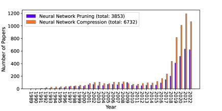
Figure 1: The number of papers for neural network pruning and compression from 1988-2022.

This survey aims to provide a comprehensive overview of deep neural network pruning to diverse readers. We review representative pruning methods, propose a new taxonomy, conduct a comprehensive analysis of how different pruning manners behave in practice and give practitioners who wish to utilize pruning recommendations on choosing a suitable pruning method for different requirements. Our contributions are as follows:

(1) Comprehensive review. To our best knowledge, this survey is the most comprehensive overview of modern deep neural network pruning techniques. It distills ideas from over 300 related academic papers and establishes a new taxonomy, as shown in Fig. 2. In addition, we provide detailed descriptions of the representative methods for each class of pruning methods.

TABLE I: Representative surveys and descriptions.

Survey	Main work description	Year
[36]	survey of pruning methods	1993
[37]	overview 81 papers and propose ShrinkBench,	2020
	an open-source framework for evaluation
[28]	pruning+weight sharing+low-rank matrix+	2020
	KD+quantization
[30]	pruning criteria+procedure	2020
[8]	pruning+quantization+KD+low-rank factor.	2020
[27]	pruning+KD+NAS+Tensor-Decompose	2020
	+quantization+hardware acceleration
[31]	work on sparsity in deep learning up to 2020	2021
[34]	overview pruning at initialization	2022
[29]	pruning+KD+NAS+quantization	2022
	+Tensor-Decompose+hardware accel.
[35]	structured pruning	2023

(2) Comparative experiments and analysis. We conduct a comparative analysis of seven pairs of contrast settings for pruning and emerging advances, including different levels of supervision for pruning. Unlike the existing surveys on pruning, this paper conducts experiments and related discussions.

(3) Collection of abundant resources. We summarize miscellaneous pruning applications and provide benchmark datasets, networks, and evaluations on different applications. Our collected resources in Appendix B could guide researchers and practitioners to understand, utilize, and develop different network pruning methods for various requirements. The ongoing updates of representative pruning efforts are available at https://github.com/hrcheng1066/awesome-pruning.

(4) Recommendations and future directions. This survey provides valuable recommendations on choosing an appropriate pruning method for different application requirements and highlights promising future research directions.

The remainder of this survey is organized as follows. First, in Section 2, we explain commonly used terms and establish a clear taxonomy of pruning. Section 3 - 6 offer an overview of speedup, when to prune, and how to prune, followed by a comprehensive comparative analysis of different kinds of pruning methods in Section 7. Section 8 discusses integrating pruning with other compression methods. Some practical recommendations for choosing pruning methods and future directions are provided in Section 9. We conclude this paper in Section 10.

2 Background

In this section, we first list the commonly used terms and notations in this literature. Then the hierarchical structure of this survey is shown in Fig. 2.

2.1 Terms and Notations

The following subsection presents the commonly used terms in pruning literature. It is worth mentioning that some terms (e.g., compression ratio) have a variety of definitions in prior works. We then provide several definitions used in different literature. In addition, for better readability, we list the notations used in this paper in Table II.

TABLE II: Notations and descriptions.

Notation	Description
$\mathbf{x}$	Input data
$\mathcal{D}$	Dataset
$f$	A network function
$N$	The number of samples in a dataset
$\mathbf{w}$	The model weights
$\mathbf{w}_{t}$	The weights after training $t$ epochs
$\mathcal{F}_{i,j}$	The $j$-th filter of the $i$-th layer
$c_{i}$	The $i$-th channel of a network
$\ell$	Standard loss function, e.g., cross-entropy loss
$\mathcal{L}$	Target loss function
$L$	Total number of layers in a network
$\odot$	Element-wise multiplication
$\lambda$	A balance factor
$\boldsymbol{\gamma}$	A scaling factor vector
$\mathbf{m}$	The masks of weights (or filters, channels, etc.)
$\mathcal{R}(\cdot)$	Regularization term
$\Delta\mathcal{L}$	Loss change
$c_{out}^{(i)}$	The number of filters at layer $i$
t	Threshold vector

• Prune Ratio: Prune ratio [38] denotes the percentage of weights (or channels, filters, neurons, etc.) that are removed from the dense network. In general, it can be determined in two ways: pre-defined or learning-decide.

• Compression Ratio: Compression ratio in [39, 40] is defined as the ratio of the original weight numbers to the preserved weight numbers, but in [41] it is defined as the ratio of the preserved weight numbers to the original weight numbers. For example, if 10% of weights are preserved, then the compression ratio in [40] is 10, but it is 10% in [41].

• Sparsity Ratio: Sparsity ratio or sparsity denotes the portion of zero weights (or channels, filters, neurons, etc.) in networks after pruning [42, 43]. It equals to compression ratio in [41].

• Speedup Ratio: Speedup ratio is defined as the value of the pruned number of FLOPs in [12], or MACs in [44] divided by the original number of FLOPs or MACs correspondingly. In [45], the speedup ratio is calculated by dividing the pruned number of filters in one layer by the original number of filters in that layer.

• One-shot Pruning: One-shot pruning, also called single-shot pruning in [46], scores only once and then prunes the network to the target prune ratio [47, 48].

• Iterative Pruning: Iterative pruning [10], also called greedy pruning or oracle pruning in [49], repeatedly score-prune-retrain circle multiple rounds, and each round is one iteration.

• Local Pruning: Local pruning prunes a network by subdividing all weights (or filter, channels, etc.,) into subsets (e.g., layers) and then removing a percentage of each subset [50].

• Global pruning: In contrast to local pruning, global pruning removes structures from all available structures of a network until a specific prune ratio is reached [50].

• Dynamic pruning: Dynamic pruning depends on specific inputs [51], wherein different subnetworks will be generated for each input sample.

• Static Pruning: In contrast to dynamic pruning, the pruned model is shared by different samples for static pruning [51]. In other words, the model capacities are fixed for different inputs.

• Lottery Ticket Hypothesis: Lottery Ticket Hypothesis (LTH) [47] points out that a randomly-initialized dense network $f(\mathbf{x};\mathbf{w}_{0})$ contains a sparse subnetwork $f(\mathbf{x};\mathbf{w}_{0}\odot\mathbf{m})$ which is trainable with the original weights to achieve competitive performance compared to the original networks.

• Winning Tickets: For a randomly initialized network $f(\mathbf{x};\mathbf{w}_{0})$, a winning ticket $f(\mathbf{x};\mathbf{w}_{0}\odot\mathbf{m})$ is its subnetwork that once be trained for $T$ epochs (i.e., $f(\mathbf{x};\mathbf{w}_{T}\odot\mathbf{m}$) will match the performance of the trained network $f(\mathbf{x};\mathbf{w}_{T})$ under a non-trivial prune ratio. [47].

• Layer-collapse: Layer-collapse is a phenomenon mentioned in [39], which occurs when all weights of a layer of a network are removed. It renders the network untrainable. Hayou et al. [52] given a formal definition (i.e., ill-conditioned NN) to this problem.

• Weight Rewinding: Weight rewinding [53] rewinds the weights of the subnetwork to the values in an earlier epoch in training $\mathbf{w}_{t}$, where $t<<T$.

• Learning Rate Rewinding: Learning rate rewinding, proposed in [40], trains the remained weights from the final values using the learning rate schedule for the specified number of epochs.

2.2 Taxonomy

There are three critical questions when pruning a deep neural network. (1) Whether to get universal or specific acceleration through neural network pruning? (2) When to prune the neural network? Specifically, is the neural network pruned before, during, or after training the network for static pruning or dynamic (i.e., run-time) pruning? (3) Whether to prune based on specific criteria or learn to prune? The answers to the three questions correspond to the three primary aspects of deep neural network pruning as shown in Fig. 2, respectively.

The first question is whether speedup depends on specific hardware/software. It is usually divided into three types: unstructured ([47, 46, 39]), semi-structured (also called pattern-based) ([54, 55, 56]) and structured ([57, 58, 59]). Only structured pruning can achieve universal neural network acceleration and compression without requiring special hardware or software. Conversely, both unstructured and semi-structured pruning need the support of special hardware or software.

The second question especially indicates the arrangement between pruning weights and training weights of the neural network for static pruning. According to whether pruning is performed before, during, or after training the network, static pruning arrangement can be divided into three categories: pruning before training (PBT) ([46, 39, 60, 61, 52]), pruning during training (PDT) ([62, 63, 64]), and pruning after training (PAT) ([47, 65, 66, 67]). In dynamic pruning, subnetworks are generated at run-time for each input data point.

The third question considers whether to prune neural networks with specific criteria or by learning. Criteria rely on a heuristic formula to measure the importance of each weight (or filter, channel, and so on). The commonly used pruning criteria include magnitude, norm, loss change, etc. In addition, it is also possible to prune neural networks by learning, such as pruning through sparsity regularization training or dynamic sparse training [68], etc. Whether through criteria or learning, pruning aims to determine the weights of a network that should be pruned.

The above three aspects determine the main characteristics of a pruning algorithm. Different combinations of these three aspects form different pruning methods. We provide a new taxonomy of deep neural network pruning in Section 3-6, and Section 8, as shown in Fig. 2.

3 Specific or Universal Speedup

This section categorizes deep neural network pruning into unstructured, semi-structured, and structured. The first two types correspond to specific speedup, and the third corresponds to universal speedup. In the following, we give a detailed introduction to each category.

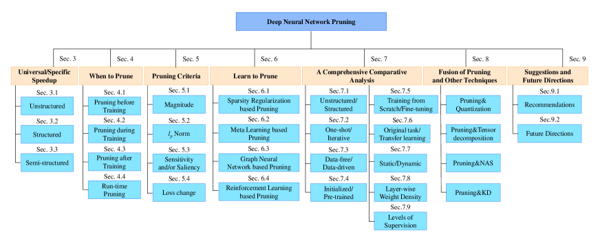
Figure 2: An overview of the hierarchical structure of the survey.

3.1 Unstructured Pruning

Unstructured pruning, also called non-structured pruning or weight-wise pruning, is the finest-grained case.

Definition 1 (Unstructured Pruning). Given neural network weights $\mathbf{w}=\{w_{0},w_{1},...,w_{K}\}$, a dataset $\mathcal{D}=\{(\mathbf{x}_{i},\mathbf{y}_{i})\}_{i=1}^{N}$ composed of input ($\mathbf{x}_{i}$), output ($\mathbf{y}_{i}$) pairs, and a desired total number of non-zero weights $k$, unstructured pruning can be written as the following constrained optimization problem [46]:

$$\begin{split}\mathop{\textrm{min}}\limits_{\mathbf{w}}\ &\mathcal{L}(\mathbf{w};\mathcal{D})=\mathop{\textrm{min}}\limits_{\mathbf{w}}\frac{1}{N}\sum_{i=1}^{N}\ell(\mathbf{w};(\mathbf{x}_{i},\mathbf{y}_{i})),\\ &\textrm{s.t.}\ \lVert\mathbf{w}\rVert_{0}\leq k.\end{split}$$ (1)

In practice, unstructured pruning usually does not directly set the weights to 0 but sets their corresponding masks (or indicators) $\mathbf{m}$ to 0 [46, 61]. In this case, unstructured pruning is regarded as applying a binary mask to each weight. Then Eq.(1) is correspondingly changed as:

$$\begin{split}\mathop{\textrm{min}}\limits_{\mathbf{w,m}}\ &\mathcal{L}(\mathbf{w}\odot\mathbf{m};\mathcal{D})=\mathop{\textrm{min}}\limits_{\mathbf{w,m}}\frac{1}{N}\sum_{i=1}^{N}\ell(\mathbf{w}\odot\mathbf{m};(\mathbf{x}_{i}.\mathbf{y}_{i})),\\ &\textrm{s.t.}\ \lVert\mathbf{m}\rVert_{0}\leq k.\end{split}$$ (2)

Generally, the network is retrained (i.e., fine-tuning or training-from-scratch) with fixed masks $\mathbf{m}$, and the masked-out weights are not involved in retraining. Fig. 3 is an example of weight-wise pruning by removing the connections of the neurons (as shown in Fig. 3(a)) or masking the weights with their corresponding masks (as shown in Fig. 3(b)), respectively. Since it can remove weights anywhere, the irregular replacement of non-zero weights leads to actual acceleration requires the support of special software and/or hardware [63, 69, 70, 51, 11]. Therefore, we classify unstructured pruning as a specific speedup technique.

3.2 Structured Pruning

Definition 2 (Structured Pruning). Given a specific prune ratio and a neural network with $S=\{s_{1},s_{2},...,s_{L}\}$, where $s_{i}$ can be the set of channels, filters, or neurons in layer $i$. Structured pruning aims to search for $S^{{}^{\prime}}=\{s_{1}^{{}^{\prime}},s_{2}^{{}^{\prime}},...,s_{L}^{{}^{\prime}}\}$ to minimize the performance degeneration and maximize the speed improvement under the given prune ratio, where $s_{i}^{{}^{\prime}}\subseteq s_{i}$, $i\in\{1,..,L\}$.

Structured pruning removes entire filters, channels, neurons, or even layers ([64]) as shown in Fig. 4(b) and can rebuild a narrow model with a regular structure. It does not need the support of special hardware and software (such as sparse convolution libraries) and can directly speed up networks and reduce the size of the neural networks [71, 50, 14, 69]. Besides, filter and channel pruning can be considered equivalent because pruning a filter in layer $i$ is equivalent to pruning the corresponding channels in layer $i+1$ [72], as shown in Fig. 4(a).

3.3 Semi-structured Pruning

To improve the flexibility of structured pruning and achieve lower accuracy drop when the pruning rate is high, some recent works ([55, 56]) introduce semi-structured pruning that is called pattern-based pruning in [56] to achieve high accuracy and structural regularity simultaneously. Various patterns can be designed; some examples are shown in Fig. 4(c). In contrast, fully structured pruning (such as channel or filter pruning) is classified as coarse-grained structured pruning ([55, 56, 73]), while semi-structured pruning is classified as fine-grained structured pruning. For example, Meng et al. [74] treat a filter as several stripes and propose to prune stripes in each filter. However, patterns used for semi-structured pruning need to be carefully designed to alleviate performance degradation and conduct specific speedup like unstructured pruning.

4 When to Prune

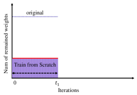
(a) SNIP [46] as an example of PBT

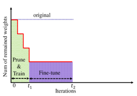
(b) FCF [91] as an example of PDT

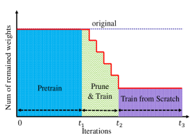
(c) LTH [47] as an example of PAT

Figure 6: The illustration of typical sparsity changes for PBT, PDT, and PAT (best view in color and zoom in). PBT is usually the cheapest, and PAT is the most expensive.

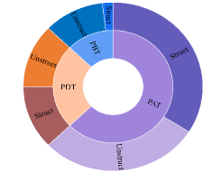
(b) Pipelines & unstruct/struct

Figure 12: Statistics of pruning literature in our survey.

This section distinguishes three pruning pipelines for static pruning, as illustrated in Fig. 5, and run-time pruning. The examples of the three pipelines of static pruning are shown in Fig. 6. The statistics of pruning literature on the three types of pipelines for static pruning are shown in Appendix B Fig. 12.

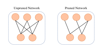
(a) From the view of neurons and connections

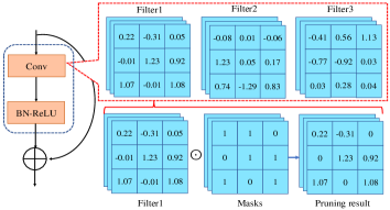
(b) From the view of weights and masks

Figure 3: The visualization of unstructured pruning. The light orange circles denote neurons.

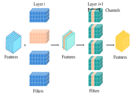
(a) Illustration of filter/channel pruning

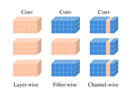
(b) Three types of structured pruning

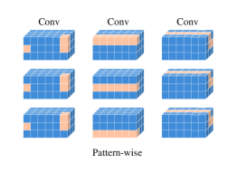
(c) Three examples of semi-struc. pruning

Figure 4: The visualization of structured and semi-structured pruning, where each Conv is composed of a specific number of little cubes, and each little cube indicates a weight. The light orange cubes denote the pruned weights.

4.1 Pruning Before Training

Pruning Before Training (PBT), also called foresight pruning [61] or pruning at initialization [46, 39], represents a class of pruning methods that use randomly initialized weights for pruning the network. The principal motivation of PBT methods is to eliminate the cost of pretraining. Without loss of generality, we define a neural network as a function $f(\mathbf{x};\mathbf{w}\odot\mathbf{m})$. The mask $\mathbf{m}$ is used for pruning initialized weights $\mathbf{w}_{0}$ sampled from a specific initialization distribution. After pruning, the network $f(\mathbf{x};\mathbf{w}_{0}\odot\mathbf{m}^{{}^{\prime}})$ is trained to converge $f(\mathbf{x};\mathbf{w}_{T}\odot\mathbf{m}^{{}^{\prime}})$ after $T$ epochs, where $\mathbf{m}^{{}^{\prime}}$ indicates the sparsity results after pruning.

PBT usually follows the two-step stages: directly prunes untrained dense network based on a specific criterion and then trains the sparse network to convergence for high performance, as illustrated in Fig. 5 (a). The second step is related to static sparse training [75] that aims to train a sparse network with a fixed sparse pattern during training. Since avoiding the time-consuming pretraining process, PBT methods bring the same gains at training and inference time.

TABLE III: Representative methods of pruning before training. “U/S” denotes unstructured or structured pruning.

Method	Criteria	U/S	Date-Free (Y/N)	One-shot (Y/N)
SNIP (2019) [46]	$\left|\nabla_{\mathbf{w}}\mathcal{L}(\mathbf{w})\odot\mathbf{w}\right|$	U	N	Y
GraSP (2020)[61]	$-(H\nabla_{\mathbf{w}}\mathcal{L}(\mathbf{w}))\odot\mathbf{w}$	U	N	Y
Smart-Ratio (2020) [60]	keep-ratios	U	Y	Y
SynFlow (2020) [39]	$\nabla_{w}\mathcal{R}_{SF}(\mathbf{w})\odot\mathbf{w}$	U	Y	N
PFS (2020) [76]	$l_{1}$-norm based sparsity regularization	S	N	N
RST (2022) [65]	$l_{2}$-norm based sparsity regularization	U	N	N

Lee et al. [46] pioneer the research of PBT and propose a Single-shot Network Pruning (SNIP) method to remove the weights whose absence leads to the slightest loss change. In [77], the authors explain the feasibility of SNIP through signal propagation, empirically find pruning damages the dynamical isometry [78] of neural networks, and propose a data-free orthogonal initialization which is an approximation of exact isometry, to prune random networks. Different from the signal propagation perspective in [77], which focuses on initialization scheme, Wang et al. [61] propose Gradient Signal Preservation (GraSP) to exploit gradient norm after pruning to prune the weights that have the least effect on the gradient flow after pruning them. Tanaka et al. [39] go a step further and point out that an effective subnetwork can be identified without training and looking at the data. They propose a data-free pruning algorithm called Iterative Synaptic Flow Pruning (SynFlow) that uses the concept of synaptic flow to consider the interaction of different layers and avoid layer-collapse with gradual pruning. In addition to data-agnostic, Su et al. [60] observe that the pruned structures are not crucial for the final performance. They propose a zero-shot data-free pruning method that randomly prunes each layer using a series of layerwise keep-ratios (i.e., smart-ratios). Gebhart et al. [79] exploit the Path Kernel (i.e., the covariance of path values in a network) based on Neural Tangent Kernel [80] to unify several initialization pruning methods, such as SNIP [46], CraSP [61], SynFlow [39], under a single framework.

Zhou et al. [81] observe that when weights are randomly initialized and fixed, the untrained network can achieve nearly $40\%$ accuracy on MNIST with a well-chosen mask. They argue that although the dense network is randomly initialized, the searching for the subnetwork serves as a kind of training. Catalyzed by [81] and inspired by Weight Agnostic Neural Networks (WANNs) [82], Ramanujan et al. [83] empirically find that with an untrained network grows wider and deeper, it will contain a subnetwork that performs equally as a trained network with the same number of parameters. Then they propose the edge-popup method to find this kind of randomly initialized subnetworks. Unlike the edge-group method never changes the weight values, Bai et al. [65] propose Dual Lottery Ticket Hypothesis (DLTH) where both the subnetwork and weights are randomly selected at initialization and propose Random Sparse Network Transformation (RST) which fixes the sparse architecture but gradually train the remained weights.

Some recent works explore why we can identify an effective subnetwork at initialization instead of depending on pretrained weights. Wang et al. [76] empirically find that directly pruning from randomly initialized weights can discover more diverse and effective pruned structures. In contrast, the pruned structures found from pretrained weights tend to be homogeneous, which hinders searching for better models. Liu et al. [75] empirically demonstrate that the network size and appropriate layer-wise prune ratios are two vital factors in training a randomly pruned network at initialization from scratch to match the performance of the dense models. For example, they find random pruning is hard to find matching subnetworks on small networks (e.g., ResNet-20 and ResNet-32) even at mild prune ratios (i.e., 10%, 20%). However, random pruning can match the dense performance on larger networks (e.g., ResNet-56 and ResNet-110) at 60%-70% prune ratios.

4.2 Pruning During Training

Pruning During Training (PDT) generally takes randomly initialized dense network $f(\mathbf{x};\mathbf{w}_{0})$ as the input model and jointly trains and prunes a neural network by updating weights $\mathbf{w}$ and masks of weights (or filters, channels) $\mathbf{m}$ during training. These dynamic schemes change the masks and get the subnetwork $f(\mathbf{x};\mathbf{w}_{t}\odot\mathbf{m}_{t})$ after $t$ iterations/epochs. After pruning, many PDT methods ([64, 84, 85, 86, 87]) directly obtain the subnetworks and do not require training-from-scratch or fine-tuning process anymore. The typical pipeline of PDT is illustrated in Fig. 5 (b), where the process denoted by the dashed arrow is optional. The PDT methods have been less explored due to the more complicated dynamic process than that of PBT and PAT methods. We summarize the main prior solutions as the three paradigms: (1) sparsity regularization based, (2) dynamic spare training based, and (3) score-based. The methods related to (1) or (3) take dense-to-sparse training, and the ones related to (2) conduct sparse-to-sparse training.

4.2.1 Sparsity Regularization based Methods

Sparsity regularization technique is commonly used in PDT methods ([88, 74]). This category of methods starts with dense networks, imposes sparse constraints on loss functions, and usually zeros out some weights or their masks during training. The main effort is to design the effective target loss function $\mathcal{L}$ with an advanced penalty scheme and efficient optimization algorithms. For example, Wen et al. [63] propose Structured Sparsity Learning (SSL) to learn a sparse structure by group LASSO [89] regularization during the training. However, SSL requires computing the gradients of the regularization term w.r.t. all the weights, which is non-trivial. Gordon et al. [90] propose MorphNet that reuses the parameters of BN and conducts sparsity regularization on these parameters. However, some networks (e.g., some VGGNets [2]) have no BN layers. Instead of reusing BN parameters, some works associate scaling factors with channels, filters, layers, etc. For example, Huang and Wang [64] propose Sparse Structure Selection (SSS) that associates scaling factors for CNN micro-structures (e.g., channels, residual blocks) and exploit sparsity regularization to force the output of the micro-structures to zero, rather than pushing the weights in the same group to zero in [63]. In addition, SSS does not require extra fine-tuning that is needed in [63]. Li et al. [91] propose factorized convolutional filter (FCF) which introduces a binary scalar to each filter and proposes a back-propagation with Alternating Direction Method of Multipliers (ADMM) [92] algorithm to train the weights and the scalars during training jointly.

4.2.2 Dynamic Sparse Training based Methods

A class of the PDT methods ([93, 94, 95, 84, 96, 97, 98]) take randomly initialized sparse network rather than dense network as the input model. Subsequently, one common method is pruning a fraction of unimportant weights followed by regrowing the same number of new weights to adjust the sparse architecture. By repeating the prune-and-grow cycle during training, this kind of method keeps searching for better sparse architecture, which is classified as dynamic sparse training in [84].

For example, Mocanu et al. [93] propose Sparse Evolutionary Training (SET) that removes the smallest positive and the most negative weights and grow new weights in random locations. Instead of pruning a fixed fraction of weights at each redistribution step, such as in SET [93], Mostafa and Wang [95] propose Dynamic Sparse Reparameterization (DSR) which uses an adaptive threshold for pruning. In addition, DSR [95] reallocates weights across layers and does not restrict to the inner-layer weight redistribution in SET [93]. Liu et al. [99] propose an ensemble method FreeTickets that ensemble sparse subnetworks created by sparse-to-sparse methods. Instead of using a random regeneration scheme, Dai et al. [94] propose a DNN synthesis tool (NeST) that stars training with a small network, adjust the subnetworks with gradient-based growth and magnitude-based pruning. Evci et al. [84] propose Rigged Lottery (RigL) that actives new connections during training by using gradient magnitude. Similarly, Liu et al. [96] propose Gradual Pruning with zero-cost Neuroregeneration (GraNet) to remove connections of networks based on their weight magnitudes and regrow connections of networks based on their gradient. They argue that even the weights with zero gradient values indicate the connection importance. Sokar et al. [100] pioneer to explore dynamic sparse training in Reinforcement Learning (RL). Graesser et al. [101] systematically investigate some dynamic sparse training methods (such as RigL [84], SET [93]) in RL.

Evci et al. [102] analyze the reasonability of dynamic sparse training. The authors find sparse networks have poor gradient flow at initialization, but dynamic sparse training significantly improves gradient flow. It could be the reason for their success.

TABLE IV: Representative methods of pruning during training. “retrain” refers to training from scratch or fine-tuning, “U/S” denotes unstructured or structured pruning.

Method	Object function/Criteria	Retrain (Y/N)	U/S
Network Slimming (2017) [62]	$\mathop{\textrm{min}}\limits_{\mathbf{w},\boldsymbol{\gamma}}\ell(\mathbf{y},f(\mathbf{x};\mathbf{w}))+\lambda\lVert\boldsymbol{\gamma}\rVert_{1}$	Y	S
SSS (2018) [64]	$\mathop{\textrm{min}}\limits_{\mathbf{w},\boldsymbol{\gamma}}\ell(\mathbf{y},f(\mathbf{x};\mathbf{w},\boldsymbol{\gamma}))+\mathcal{R}(\mathbf{w})+\lambda\lVert\boldsymbol{\gamma}\rVert_{1}$	N	S
SET (2018) [93]	$\lVert\mathbf{w}\rVert$ for drop and random for grow	N	U
DST (2020) [68]	$\mathop{\textrm{min}}\limits_{\mathbf{w},\textbf{t}}\ell(\mathbf{y},f(\mathbf{x};\mathbf{w}))+\lambda\sum_{i=1}^{L}\sum_{j=1}^{c_{out}^{(i)}}exp(-\textbf{t}_{j})$	N	S
GraNet (2021) [96]	$\lVert\mathbf{w}\rVert$ for drop and gradient for grow	N	U&S
FreeTickets (2022) [99]	$\lVert\mathbf{w}\rVert$ for drop and gradient for grow	N	U

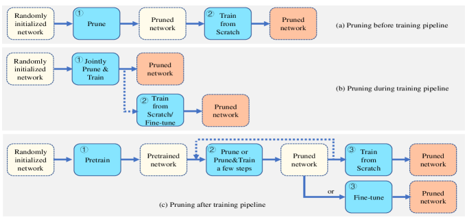
Figure 5: The typical pruning pipelines of static pruning. Dashed boxes represent models and solid boxes denote actions.

4.2.3 Score-based Methods

Some PDT methods exploit scoring criteria to prune the networks during training. He et al. [86] propose Soft Filter Pruning (SFP) filter pruning method which can train the networks from scratch and prune the networks simultaneously by using the $l_{2}$ norm of each filter as its importance. Instead of associating masks with filters, they directly set the pruned filter weights as zeros, which can be updated from zeros through the forward-backward process. Hence, the pruned filters in this epoch can be recovered in the next epoch. However, SFP requires manually preset prune ratios for each layer. He et al. [103] propose Filter Pruning via Geometric Median (FPGM) to prune the redundant filters which are nearest to the geometric median [104] of the filters within the same layer. However, FPGM also requires a pre-defined prune ratio for each layer. Liu et al. [62] propose a method called Network Slimming which introduces a scaling factor for each channel and jointly trains the weights and the scaling factors by adding the regular loss $\ell$ with sparsity regularization on the factors, and the magnitudes of these scaling factors are used as the filter scores. In practice, they directly reuse the $\gamma$ parameters in Batch Normalization (BN) [105] layers as the scaling factors.

4.3 Pruning After Training

Pruning After Training (PAT) is the most popular type of pruning pipeline because it is commonly believed that pretraining the dense network is necessary to obtain an efficient subnetwork [38]. This class of pruning methods generally follows a Pretrain-Prune-Retrain process as shown in Fig. 5 (c). (1) Pretrain a randomly initialized dense network $f(\mathbf{x};\mathbf{w}_{0})$ to converge $f(\mathbf{x};\mathbf{w}_{T})$. (2) Prune the weights (or filters, neurons, etc.) that have the least influence on the performance and fine-tune the pruned network $f(\mathbf{x};\mathbf{w}_{T}^{{}^{\prime}}\odot\mathbf{m}^{{}^{\prime}})$ for several iterations, where $\mathbf{w}_{T}^{{}^{\prime}}$ and $\mathbf{m}^{{}^{\prime}}$ are the weights and masks after pruning, respectively. Process (2) is processed at least once (i.e., one-shot pruning) or multiple times (i.e., iterative pruning). (3) Train the remained weights from scratch $f(\mathbf{x};\mathbf{w}_{0}\odot\mathbf{m}^{{}^{\prime\prime}})$ or fine-tune $f(\mathbf{x};\mathbf{w}_{T}^{{}^{\prime\prime}}\odot\mathbf{m}^{{}^{\prime\prime}})$ to recover the performance [40], where $\mathbf{w}_{T}^{{}^{\prime\prime}}$ and $\mathbf{m}^{{}^{\prime\prime}}$ are the final results of weights and masks after the overall pruning process, respectively. During the pruning process, sparsity is gradually increased until it achieves the target.

4.3.1 LTH and its Variants

Lottery Ticket Hypothesis (LTH) [47] is one of the most influential hypotheses in the neural network pruning domain. Given a pretrained network, LTH iteratively removes a percentage of the weights based on their magnitudes. After pruning, the remaining weights are retrained from scratch with the original initialization, rather than random reinitialization, to match the original networks’ accuracies. It challenges the commonly believed paradigm that the pretrained weights must be used for retraining and conjectures the existence of an independently trainable sparse subnetwork from a dense network. Inspired by LTH, there are various follow-up works to identify wider tickets and understand LTH better, which can be classified into four main classes: (1) proposing a stronger lottery ticket hypothesis, (2) exploring the transferability of LTH, (3) generalizing LTH to other contexts, (4) theoretical justification, and (5) revisiting and questioning LTH.

(1) Some recent works ([106, 107, 108]) prove stronger hypothesis than LTH [47]. For example, Diffenderfer and Kailkhura [108] propose a stronger Multi-Prize LTH, which claims that winning tickets can be robust to extreme forms of quantization (i.e., binary weights and/or activations). Based on this, they propose a Multi-Prize Tickets (MPTs) algorithm to find MPTs on binary neural networks for the first time.

(2) Some literature ([109, 110, 111, 67]) studies the transferability of a winning ticket found in a source dataset to another dataset, which provides insights into the transferability of LTH. For example, S. Morcos et al. [109] find OneTicket that can generalize across a variety of datasets and optimizers within the natural image domain. Mehta [110] propose the ticket transfer hypothesis and transfer winning tickets for different image classification datasets.

(3) In addition to image classification, LTH is extended to numerous other contexts, such as node classification and link prediction ([67]) and vision-and-language ([111]). For example, Chen et al. [67] pioneer to generalize LTH to Graph Neural Networks (GNNs) [112] and propose Graph Lottery Ticket (GLT).

TABLE V: Representative methods of pruning after training. “U/S” denotes unstructured or structured pruning.

Method	Object function/Criteria	U/S
Auto-Balance (2018) [113]	score($\mathcal{F}_{i,j}$)=$\lVert\mathcal{F}_{i,j}\rVert_{1}$	S
LTH (2019) [47]	score($w_{i}$)=$\lVert w_{i}\rVert_{1}$	U
Taylor-FO-BN (2019) [114]	score($w_{i}$)=$(\nabla_{w_{i}}\ell\odot w_{i})^{2}$	S
SSR (2019) [115]	$\mathop{\textrm{min}}\limits_{\mathbf{w}}\frac{1}{N}\sum_{i=1}^{N}\ell(\textbf{y}_{i},f(\textbf{x}_{i},\mathbf{w}))+\lambda\mathcal{R}(\mathbf{w})$	S
GReg (2021) [116]	score($\mathcal{F}_{i,j}$)=$\lVert\mathcal{F}_{i,j}\rVert_{1}$	U&S
GFP (2021) [71]	score($c_{i}$)=$\sum_{a=1}^{N}(\nabla_{m_{i}}\ell_{a})^{2}$ or score($c_{i}$)=$\sum_{a=1}^{N}(\sum_{g\in Group}\nabla_{m_{i}^{g}}\ell_{a})^{2}$	S

(4) On one hand, some literature ([117, 118]) analyzes the reasons why LTH [47] is able to win. For example, Zhang et al. [117] exploit dynamical systems theory and inertial manifold to theoretically verify the validity of LTH. Evci et al. [102] observe that the success of LTH lies in effectively re-learning the original pruning solution they are derived. Zhang et al. [118] pioneer to provide formal justification of the improved generalization of winning tickets observed from experimental results in LTH.

(5) On the other hand, some recent works ([119, 120, 38]) revisit and challenge the existence of LTH. For example, Ma et al. [119] provide a more rigorous definition of LTH for precisely identifying winning tickets and find that whether and when the winning tickets can be identified highly replies on the training settings, such as learning rate, training epochs, and the architecture characteristics, like network capacities and residual connections. It is more likely to find winning tickets by using a small learning rate or an insufficient number of training epochs.

It is worth pointing out that in some works [34, 16], LTH [47] is classified as a PBT method. However, LTH selects masks based on a pretrained network, which does not conform to the definition of PBT that attempts pruning the initialized network before training. Therefore, it is more reasonable to classify LTH as a PAT method.

4.3.2 Other score-based Methods

The most straightforward and intuitive way to select pruning candidates is to evaluate them based on their norms. For example, Han et al. [11] propose to measure the weight importance by its absolute value. Li et al. [69] score every filter in each layer by calculating the sum of its weights’ $l_{1}$-norm. In addition to norm-based criteria, evaluating loss change with and without the weights is also popular. For example, Nonnenmacher et al. [50] propose Second-order Structured Pruning (SOSP) to selectively zero out filter masks to minimize the effects of the loss change from removing some filters. Discrimination-aware Channel Pruning (DCP) [121] selects the most discriminative channels by minimizing a joint loss which includes the regular loss with the discrimination-aware loss. Many works ([116, 58, 113, 14]) evaluate the importance of weights (or filters, neurons, etc.) locally within each layer. The key drawback of these methods is that the local ranking makes it hard to decide the overall optimal sparsity, and the pre-defining prune ratio per layer may be non-trivial and sub-optimal. Some works ([122, 43, 123]) are presented to cope with this problem. For example, Chin et al. [122] proposes Learned Global Ranking (LeGR) to learn the filter ranking globally across layers. Liu et al. [71] propose Group Fisher Pruning (GFP) to apply the Fisher information to evaluate the importance of a single channel and coupled channels.

4.3.3 Sparsity Regularization based Methods

Some works ([124, 125, 115, 126]) exploit sparsity regularization technique. For example, He et al. [124] propose an alternative two-step algorithm that introduces a scalar mask to each channel of a pretrained CNN model and selects redundant channels based on LASSO regression [127] and reconstructs the outputs with unpruned channels with linear least squares. Energy-Constrained Compression (ECC) [128] builds the energy consumption model via a bilinear regression function. Network Pruning via Performance Maximization (NPPM) [129] trains a performance prediction network and uses it as a proxy of accuracy to guide searching for subnetworks based on regularization penalty. Fang et al. [44] develop a general method called DepGraph to analyze dependencies of various network structures (e.g., CNNs, RNNs, GNNs, Transformers) and propose a structured pruning based on sparsity regularization. Some methods ([116, 58, 113, 44]) select important weights (or filters, neurons, etc.) by combining norm-based criteria and sparsity regularization.

4.3.4 Pruning in Early Training

Instead of fully training a network from $f(\mathbf{x};\mathbf{w}_{0})$ to $f(\mathbf{x};\mathbf{w}_{T})$, this class of methods explore the network architecture by training a network only for a few iterations or epochs, i.e., $f(\mathbf{x};\mathbf{w}_{t})$, where $t<<T$. For example, You et al. [130] propose Early-Bird (EB) tickets which indicate that winning tickets can be identified at the early training stage via inexpensive training schemes (e.g., early stopping and low-precision training) at large learning rates and achieve similar performance to the dense network. Inspired by [130], Chen et al. [131] propose EarlyBERT that identifies structured winning tickets in the early stage of BERT [132] training. Frankle et al. [53] find that, in large-scale settings (such as ResNet-50 and Inception-v3 on ImageNet), the subnetworks that exhibit stability to SGD noise are able to reach full accuracy early in training.

4.3.5 Post-Training Pruning

In contrast to the general PAT methods that follow the Pretrain-Prune-Retrain procedure, recently proposed post-training pruning simplifies the three-step process as Pretrain-Prune. It involves pruning a pre-trained model $f(\textbf{x};\textbf{w}_{T})$ without retraining, with a negligible accuracy loss. This class of pruning methods is particularly attractive for billion-parameter models because retraining such pruned models after pruning is still very expensive. For example, Frantar and Alistarh [15] propose an unstructured post-training pruning method called SparseGPT. By simplifying the pruning problem to an approximate sparsity regression, the authors prune GPT family models at least 50% sparsity at minor accuracy loss without retraining. To our best knowledge, it is the first pruning method specifically designed for GPT family models. Kwon et al. [133] propose a structured post-training pruning framework for Transformers, which includes three steps: Fisher-based mask search, Fisher-based mask rearrangement, and mask tuning. Without retraining, this framework can prune Transformers on one GPU in less than 3 minutes.

4.4 Run-time Pruning

The prior works on pruning usually focus on static pruning methods where the pruned model is reused for different inputs. In contrast, some methods prune neural networks according to individual inputs dynamically, namely run-time pruning [134]. This line of work is based on the premise that for a given task, the difficulty of producing accurate output can vary, implying the necessity of model capacities for different inputs is different [51]. For example, Rao et al. [134] propose a Runtime Network Routing (RNR) framework to conduct dynamic routing based on the input image and current feature maps and select an optimal path subset for compression. Tang et al. [51] point out that the importance of channels highly depends on the input data and propose to generate different subnetworks for each instance. At inference, only channels with saliencies larger than the threshold need to be computed, and the redundant features are skipped. Hua et al. [135] exploit input-specific characteristics and propose CGNets to predict the unimportant regions by the partial sum of the output activation by performing convolution on a subset of input channels. Gao et al. [136] propose Feature Boosting and Suppression (FBS) to predict the saliency of channels and skip those with less contribution to the classification results at run-time. Fire Together Wire Together [33] poses the dynamic model pruning as a self-supervised binary classification problem. Meng et al. [137] propose Contrastive Dual Gating (CDG) that is another self-supervised dynamic pruning method by using contrastive learning [138].

5 Pruning Criteria

In this section, we summarize some commonly used pruning criteria that are used to evaluate the importance of weights (or filters, neurons, etc.) from different perspectives, including magnitude ([10, 139, 140, 141]), norm ([86, 69]), saliency and/or sensitivity ([85, 142, 143]), loss change ([142, 144, 13, 50, 71]). There is no rigid boundary between these criteria but a different emphasis.

5.1 Magnitude-based Pruning

[26] is one of the earliest works that propose magnitude-based pruning to reduce hidden units. Han et al. [11] popularize magnitude-based pruning for deep neural networks, which prunes the lowest-magnitude weights. It is based on the assumption that the weights with smaller absolute values tend to have the least influence on the network’s output. The formulation is defined as

$$m_{i}=\begin{cases}1:if\ \lVert w_{i}\rVert_{1}\geq a\\ 0:if\ \lVert w_{i}\rVert_{1}<a\end{cases},$$ (3)

where $a$ is a threshold.

Magnitude-based criteria can be applied for either unstructured ([10, 47, 139, 145, 146, 147]) or structured pruning ([69, 94, 148]). For example, Li et al. [69] score the filters by calculating the sum of their absolute magnitude of weights. In addition, magnitude-based criteria can be combined with global/local, one-shot/iterative schedules. For example, the works in [149] and [150] propose magnitude-based iterative global pruning methods. Singh Lubana and P. Dick [140] argue that magnitude-based pruning results in faster model convergence than magnitude-agnostic methods.

5.2 $l_{p}$ Norm

Some methods ([86, 69]) use the $l_{p}$ norm to evaluate the importance of weights (or filters, channels, etc.). For example, He et al. [86] exploit $l_{p}$ norm to evaluate the importance of the filter $\mathcal{F}_{i,j}$ as Eq.(4).

$$\lVert\mathcal{F}_{i,j}\rVert_{p}=\left(\sum_{n=1}^{c_{in}^{(i)}}\sum_{k_{1}=1}^{k^{(i)}}\sum_{k_{2}=1}^{k^{(i)}}\left|\mathcal{F}_{i,j}(n,k_{1},k_{2})\right|^{p}\right)^{\frac{1}{p}},$$ (4)

where $k^{(i)}$ is the kernel size of layer $i$ in a network and $c_{in}^{(i)}$ is the number of channels at layer $i$. The filters with small $l_{p}$ norm are more likely pruned than those of higher $l_{p}$ norm. Some norm-based pruning methods ([69]) use $l_{1}$ norm as the importance metric. In this case, these methods also belong to magnitude-based pruning methods. In addition, the importance value is often optimized with norm-based sparsity regularization ([113]) that is discussed in 6.1.

5.3 Sensitivity and/or Saliency

Some works ([151, 143, 85]) utilize sensitivity and/or saliency to evaluate the importance of weights (or channels, filters, etc.). The definition of sensitivity or saliency may be different in prior works. For example, LeCun et al. [151] define weight saliency as the loss change induced by pruning that weight. SNIP [46] proposes a saliency criterion called connection sensitivity criterion as the normalized magnitude of the derivatives $g_{j}$:

$$s_{j}(\mathbf{w};\mathcal{D})=\frac{\left|g_{j}(\mathbf{w};\mathcal{D})\right|}{\sum_{k=1}^{m}\left|g_{k}(\mathbf{w};\mathcal{D})\right|},$$ (5)

where $s_{j}$ is the sensitivity of the weight $j$, $\mathbf{w}$ is the networks weights, $g_{j}$ is the derivative of the loss $L(\mathbf{w}\odot\mathbf{m})$ w.r.t. $m_{j}$. The higher the sensitivity of weight, the more important it is. VCP [85] reformulates the BN layer by extending the scale factor $\gamma$ on shift term $\beta$ that is treated as channel saliency. They reformulate BN as follows:

$$\mathbf{x}_{out}=\gamma\cdot BN(\mathbf{x})+\tilde{\beta},$$ (6)

where $\tilde{\beta}=\gamma\cdot\beta$. Rather than relying on the value of $\gamma$, VCP prunes unimportant channels based on $\gamma$’distributions.

5.4 Loss Change

It is a popular criterion to measure the importance of weight (or filter, channel, etc.) by evaluating the loss change of the network with and without it. For simplicity, we take filter importance evaluation as an example. Since reevaluating the whole network’s performance after removing filters one by one is nontrivial, some researchers ([13, 50, 71]) approximate a filter’s importance in a Taylor expansion based way.

The first-Order Taylor expansion is the most commonly used method for measuring the loss change. The loss change with a small perturbation at $\mathbf{w}$ is defined as follows:

$$\Delta\mathcal{L}=\mathcal{L}(\mathbf{w}+\Delta\mathbf{w})-\mathcal{L}(\mathbf{w})=\nabla_{\mathbf{w}}\mathcal{L}\ \Delta\mathbf{w}.$$ (7)

For example, GBN [13] introduces the scaling factors $\boldsymbol{\lambda}$ to the BN and exploits the first-order Taylor expansion to estimate the loss change $\Delta\mathcal{L}$ caused by setting some scaling factors to zero as follows:

$$\Delta\mathcal{L}(\boldsymbol{\lambda})=\left|\boldsymbol{\lambda}\nabla_{\boldsymbol{\lambda}}\mathcal{L}-R_{1}(\boldsymbol{\lambda})\right|\approx\left|\boldsymbol{\lambda}\nabla_{\boldsymbol{\lambda}}\mathcal{L}\right|=\left|\frac{\partial\mathcal{L}}{\partial\boldsymbol{\lambda}}\boldsymbol{\lambda}\right|,$$ (8)

where $R_{1}(\boldsymbol{\lambda})$ is the Lagrange remainder. The importance score of the $i$-th filter is defined as

$$\textrm{Score}(\mathcal{F}_{i})=\mathop{\sum}\limits_{(\mathbf{x},\mathbf{y})\in\mathcal{D}}\left|\frac{\partial\mathcal{L}(\mathbf{y},f(\mathbf{x};\mathbf{w})}{\partial\lambda_{i}}\lambda_{i}\right|,$$ (9)

where $\lambda_{i}$ is the scalar factor of the $i$-th filter.

The second-order Taylor expansion of the loss function is early used in [151] for removing unimportant weights and gradually exploited in many subsequent methods ([50, 71]), which includes the first-order (gradient) term, the second-order (Hessian) term, and the higher-order terms are neglected. Without loss of generality, the approximation of the loss change leads to

$$\mathcal{L}(\mathbf{w}+\Delta\mathbf{w})-\mathcal{L}(\mathbf{w})=\nabla_{\mathbf{w}}\mathcal{L}\ \Delta\mathbf{w}+\frac{1}{2}\Delta\mathbf{w}^{T}H\Delta\mathbf{w},$$ (10)

where $H=\nabla_{\mathbf{w}}^{2}\mathcal{L}(\mathbf{w})$.

For example, GFP [71] applies the second-order Taylor expansion to approximate the loss change when removing a channel (setting its mask to 0):

$$s_{i} =\Delta\mathcal{L}=\mathcal{L}(\mathbf{m}-\textbf{e}_{\textbf{i}})-\mathcal{L}(\mathbf{m})\approx-\textbf{e}_{\textbf{i}}^{T}\nabla_{\mathbf{m}}\mathcal{L}+\frac{1}{2}\textbf{e}_{\textbf{i}}^{T}(\nabla_{\mathbf{m}}^{2}\mathcal{L})\textbf{e}_{\textbf{i}}$$ (11)

$$=-\textbf{e}_{\textbf{i}}^{T}g+\frac{1}{2}\textbf{e}_{\textbf{i}}^{T}H\textbf{e}_{\textbf{i}}=-g_{i}+\frac{1}{2}H_{ii},$$

where $\textbf{e}_{\textbf{i}}$ is the one-hot vector of which the $i$-th entry equals one, $g$ is the gradient of loss function $\mathcal{L}$ w.r.t. $\mathbf{m}$.

6 Learn to Prune

In this section, we present some methods through learning to prune networks, including sparsity regularization ([124, 62, 64, 152, 153]) and some pruning methods based on meta-learning ([87, 152]), graph neural network ([154]), and reinforcement-learning ([43, 134]).

6.1 Sparsity Regularization based Pruning

Sparsity regularization based pruning learns the weights and their masks by solving the following problem:

$$\mathop{\textrm{min}}\limits_{\mathbf{w},\mathbf{m}}\mathcal{L}(\mathbf{w},\mathbf{m})\\ ,$$ (12)

where $\mathcal{L}=\ell(\mathbf{w},\mathbf{m})+\lambda\mathcal{R}(\cdot)$. One common way of this class of pruning methods is introducing scaling factor vector $\boldsymbol{\gamma}$ for weights (or channels, filters, etc.). The network weights and the scaling factors $\boldsymbol{\gamma}$ are trained jointly with sparsity regularization imposed on the latter. The magnitude of the scaling factors is treated as the important scores. Specifically, $\mathcal{L}$ in Eq. 12 can be exemplified as follows:

$$\mathcal{L}=\frac{1}{N}\sum_{i=1}^{N}\ell(\mathbf{y}_{i},f(\mathbf{x}_{i};\mathbf{w},\boldsymbol{\gamma}))+\lambda\sum_{\gamma_{i}\in\boldsymbol{\gamma}}\mathcal{R}(\gamma_{i}).$$ (13)

For example, He et al. [124] cast channel selection as reconstruction error minimization of feature maps and formulate the channel pruning problem as follows:

$$\mathop{\textrm{min}}\limits_{\beta,\mathbf{w}}\frac{1}{2N}\lVert\mathbf{y}-\sum_{i=1}^{c}\beta_{i}X_{i}W_{i}^{T}\rVert_{F}^{2}+\lambda\lVert\beta\rVert_{1},$$ (14)

$$\textrm{subject to}\ \lVert\beta\rVert_{0}\leq c^{\prime},\forall i\ \lVert W_{i}\rVert_{F}=1.$$

where $\lVert\cdot\rVert_{F}$ is Frobenius norm, $X_{i}$ is $N\times k_{h}k_{w}$ matrix from $i$-th channel of input $\mathbf{x}$, $W_{i}$ is $n\times k_{h}k_{w}$ weights from $i$-th channel of $\mathbf{w}$, $k_{h}$ and $k_{w}$ are the kernel height and width, respectively. $N$, $c$, $c^{\prime}$, and $n$ are the number of samples, channels, retained channels, and filters, respectively. To solve this problem, He et al. [124] use LASSO regression [127] and greedy strategy to select the unimportant channels.

6.2 Meta-Learning based Pruning

Some works ([87, 152]) adopt meta-learning to prune models. For example, MetaPruning [87] trains a meta network, PruningNet, to predict weights for different pruned networks. The PruningNet takes a network encoding vector $(v_{1},v_{2},...,v_{L})$ as input and outputs the weights $\mathbf{w}$ of the pruned network:

$$\mathbf{w}=\textrm{PruningNet}(v_{1},v_{2},...,v_{L}),$$ (15)

where $v_{i}$ is the number of the channels for $i$-th layer. The weights and the corresponding accuracy of each pruned network are obtained by inputting the network encoding into the fully trained PruningNet. Considering the huge search space of network encoding vectors, the pruned network is found by evolutionary search under the constraints.

6.3 Graph Neural Network based Pruning

Any network can be viewed as a graph. GraphPruning [154] applies graph convolution to model compression for the first time. Specifically, GraphPruning designs a graph aggregator $G$ with weights $\mathbf{\theta}_{G}$ combined with the Fully Connected (FC) layers to generate the weights $\mathbf{w}=(\mathbf{w}^{(1)},\mathbf{w}^{(2)},...,\mathbf{w}^{(L)})$ of the Pruned Network as follow:

$$(n_{1},n_{2},...,n_{L})=G(b_{1},b_{2},...,b_{L}|\mathbf{\theta}_{G}),$$ (16)

$$\mathbf{w}^{(i)}=FC_{i}(n_{i}|\mathbf{\theta}_{i}),$$

where $b_{i}\in R^{1\times 7}$ denotes the embedding features of $i$-th node, $n_{i}$ is the $i$-th column of output with the graph aggregator, $\theta_{i}$ is the weights of the $i$th FC layer, and $\mathbf{w}^{(i)}$ is the weights of the $i$-th pruned layer of the pruned network. Then the pruned network is fully trained on the dataset. Herein, the graph aggregator is responsible for extracting high-level features for each node, while each FC layer is used to generate reasonable weights for the pruned network. Afterward, the best configuration of the pruned network under computational constraints is searched by RL methods, during which the weights of the graph aggregator and FCs are not updated.

6.4 Reinforcement Learning based Pruning

Rather than using RL to search the best configurations of the pruned networks in [154], some AutoML pruning methods ([43, 134]) adopt RL to compress models automatically. For example, He et al. [43] propose AutoML for model compression (AMC) method that is based on Q-learning, a kind of RL, to concern how an agent should take actions in order to maximize the cumulative reward. Specifically, He et al. [43] design the Deep Deterministic Policy Gradient (DDPG) agent to receive an embedding state $s_{i}$ of layer $l_{i}$ from the environment and output a sparsity ratio as action $a_{i}$. Then layer $l_{i}$ is compressed with $a_{i}$ using a specific compression method (such as a channel pruning method). After that, the agent moves to layer $l_{i+1}$ and does the same work as layer $l_{i}$ until the final layer $l_{L}$. The update process is as follows:

$$Loss=\frac{1}{N}\sum_{i=1}^{N}(y_{i}-Q(s_{i},a_{i}|\mathbf{w}^{Q}))^{2},$$ (17)

$$y_{i}=r_{i}-b+\gamma Q(s_{i+1},\mu\ (s_{i+1})|\mathbf{w}^{Q}),$$

where $b$ is the baseline reward, $\gamma$ is a discount factor used to avoid over-prioritizing short-term rewards, $\mathbf{w}^{Q}$ is the weights of the network $Q$ following Block-QNN [155], and $r_{i}$ is the reward of the whole trajectory for the $i$-th sample.

He et al. [43] observe that Error is inversely-proportional to $log(\textrm{FLOPs})$ or $log(\#\textrm{Param})$. Based on this observation, the reward function is defined as:

$$\textrm{R}_{\textrm{FLOPs}}=-\textrm{Error}\cdot log(\textrm{FLOPs}),$$ (18)

$$\textrm{R}_{\textrm{Param}}=-\textrm{Error}\cdot log(\#\textrm{Param}).$$

This reward function provides an incentive for reducing FLOPs or the number of network parameters.

7 A Comprehensive Comparative Analysis

In this section, we focus on a comparative analysis of how to behave in different pruning manners, including seven pairs of contrast settings for pruning, the different layer-wise densities of networks, and different levels of supervision for pruning. We also conduct comparative experiments to examine some pruning methods for VGGNet [2]/ResNet [6] on CIFAR-10 [156]/CIFAR-100 [156] under different contrast settings. The experimental settings refer to Appendix A.

7.1 Unstructured vs. Structured Pruning

Unstructured pruning methods ([70, 11]) remove weights anywhere and can achieve high prune ratios with little impact on accuracy. In contrast, structured pruning ([71, 50, 13]) conducts pruning at entire filters (or channels, neurons, blocks, layers, etc.), which results in really compressed network and accelerated inference, but the accuracy is more likely lower than that of unstructured pruning under the same prune ratio, weight-level scoring, pipeline, and learning schemes. The possible reason is that unstructured pruning only focuses on the importance of a single weight, while structured pruning forces structural coupling, which demands the simultaneous pruning of multiple layers and expects all removed weights to be consistently unimportant. However, meeting the consistency of unimportant weights under the structural coupling constraints is challenging. The advantages and disadvantages of unstructured and structured pruning are briefly summarized in Table VI. We prune VGG-16 on CIFAR-10 [156] in 3 random runs and report the best results to compare unstructured and structured pruning of SNIP [46] and GraSP [61]. The vanilla SNIP and GraSP are unstructured pruning, denoted by SNIP-unstruct and GraSP-unstruct in Table VII, respectively. To prune channels, after scoring each weight by vanilla SNIP or GraSP, the sum of the weight-level scores in each channel is calculated as its importance score. As shown in Table VII, for SNIP and GraSP, Top-1 accuracy of unstructured pruning is generally better than their corresponding structured pruning under the same prune ratio of weights.

TABLE VI: Advantages and disadvantages of unstructured and structured pruning.

	Unstructured	Structured
High sparsity with	✔	hard
minor accuracy drop
Speedup w/o specific hardware	hard	✔
(e.g., FPGAs or ASICs)
Speedup w/o specific software	hard	✔
(e.g., sparsity CNNs libraries)
Really compressed with	hard	✔
significant acceleration
Structure coupling	✗	✔

TABLE VII: Top-1 accuracy of unstructured and structured pruning for VGG-16. The best results are shown in bold.

Dataset	CIFAR-10		CIFAR-100
Parameters $\downarrow$ (%)	10	40	10	50
SNIP-unstruct [46]	93.84	93.73	73.09	72.67
SNIP-struct	93.74	93.71	72.82	70.68
GraSP-unstruct [61]	93.58	93.18	72.46	71.42
GraSP-struct	93.67	93.04	72.43	71.30

7.2 One-shot vs. Iterative Pruning

One-shot pruning methods score once and then prune the network to a target prune ratio. Conversely, the iterative pruning methods alternately process the score-prune-retrain cycle until achieving the target prune ratio. As a result, the pruning cost in one-shot methods usually can be negligible, which greatly saves pruning efforts. However, this kind of method is not friendly to those significant weights whose importance is not immediately apparent at the beginning [109]. Hence, one-shot pruning generally requires more carefully designed scoring criteria to match the performance of the original network. In addition, the results in [39] show that one-shot pruning may more easily suffer from layer-collapse, resulting in a sharp accuracy drop. In contrast, iterative methods require more pruning cost but generally yield better accuracy [13, 69, 120, 110, 157].

Lin et al. [97] analyze the difference between one-shot and iterative pruning methods from the perspective of stochastic gradient. Their results show that the iterative pruning method computes a stochastic gradient at the pruned model and takes a step that best suits the compressed model. In contrast, one-shot pruning method computes a stochastic gradient at the original weights and moves towards the best dense model.

We prune VGG-16 and ResNet-32 on CIFAR-10 by SynFlow [39] and Magnitude-based pruning (For simplicity, it will be referred to as Magnitude in the following.) under one-shot or iterative pruning, respectively. As illustrated in Fig. 7, Top-1 accuracy of iterative pruning is generally better than the corresponding one-shot pruning.

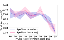
(a) SynFlow on VGG-16

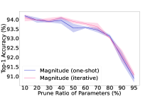
(b) Magnitude on ResNet-32

Figure 7: One-shot vs. iterative pruning on CIFAR-10. Shaded regions indicate standard deviation based on three independent runs (best view in color).

7.3 Data-free vs. Data-driven Pruning

Most of the existing pruning works ([71, 50, 46]) belong to data-driven methods, and only a few methods ([39, 60, 158, 159]) are data-free. Data is generally believed to be essential for finding good subnetworks. We prune VGG-16 on CIFAR-10 and SVHN by two data-free pruning methods (i.e., SynFlow [39] and Smart-Ratio [60]) and two data-driven methods (i.e., SNIP [46] and Magnitude). Both CIFAR-10 and SVHN are 10-class datasets. As shown in Fig. 8, the prune ratio per layer of VGG-16 by SynFlow or Smart-Ratio on CIFAR-10 is the same as the prune ratio of the corresponding layer on SVHN. However, the prune ratio per layer differs when SNIP or Magnitude prunes VGG-16 on CIFAR-10 and SVHN. Especially for Magnitude, the prune ratios of lower layers on CIFAR-10 are different from those on SVHN. The results in Table VIII are the best in three random runs and show that although data-free methods achieve good Top-1 accuracy on CIFAR-10 [156], SVHN and CIFAR-100 [156] with 50% or 90% parameters pruned, the data-driven methods outperform in most cases. Among these methods, SNIP performs best. Although it only uses a small number of randomly chosen samples (i.e., one sample per class) to calculate weight scores, the data is essential for SNIP. When it gets random inputs, as denoted by SNIP (data-free), its Top-1 accuracy has generally dropped.

TABLE VIII: Top-1 accuracy (%) of data-free and data-driven pruning methods for VGG-16. The original Top-1 accuracy on CIFAR-10, SVHN, and CIFAR-100 are 93.76%, 96.36%, and 73.22%, respectively. The best results are shown in bold.

Dataset	CIFAR-10		SVHN		CIFAR-100
Parameters $\downarrow$ (%)	50	90	50	90	90	95
Smart-Ratio [60]	93.71	93.20	96.34	96.23	71.37	70.16
SynFlow [39]	93.74	93.26	96.28	96.34	71.03	69.16
SNIP (data-free)	93.90	93.20	96.37	96.29	71.46	70.23
SNIP [46]	93.70	93.40	96.39	96.60	71.65	70.32
Magnitude	93.65	93.18	96.23	96.26	71.15	70.35

7.4 Pruning on Initialized vs. Pretrained Weights

Frankle et al. [48] find the subnetworks obtained by pruning on randomly initialized weights (such as SNIP [46], GraSP [61], SynFlow [39]) are robust to the ablation treatments (i.e., randomly shuffling the mask positions within each layer or reinitializing weights while keeping masks unchanged). To find the reason behind such immunity, Singh and Liu [160] use the Wasserstein distance to measure distributional similarity and find that the remained weights’ distribution is changed minimally with these ablations, which reinforces keeping similar performances. In contrast, Su et al. [60] find the subnetworks achieved by pruning on pretrained weights, such as LTH [47], are sensitive to these ablations. Qiu and Suda [161] claim that training weights can be decoupled into two dimensions: the locations of weights and their exact values, among which the locations of weights hold most of the information encoded by the training. Wolfe et al. [162] theoretically analyze the impact of pretraining on the performance of a pruned subnetwork. Although pretraining is crucial for PAT methods, it does not always bring benefits. We conduct some experiments to explore whether the pretrained weights facilitate PBT methods to find better subnetworks. The results in Fig. 9 show that for both SynFlow [39] and SNIP [46], pruning on the pretrained weights does not guarantee improved Top-1 accuracy. The results are worse for some prune ratios of weights.

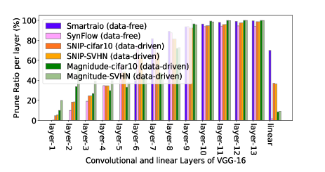
Figure 8: An illustration of the architectures of VGG-16 with 90% prune ratio of weights through data-free and data-driven pruning on CIFAR-10 and SVHN.

7.5 Training from Scratch vs. Fine-tuning

After pruning, many pruning methods require training the subnetwork for several epochs to regain performance. Le and Hua [163] argue that retraining is essential to recover loss accuracy in pruning. Generally, retraining can be divided into two types: training from scratch or fine-tuning. There has been debate over whether fine-tuning is more powerful than training from scratch to recover accuracy. On the one hand, Liu et al. [38] find that for ResNet, VGG, and other standard structures on ImageNet, training the subnetworks with new random initialization can achieve better performance than fine-tuning them. On the other hand, Li et al. [69] observe that training a subnetwork from scratch performs worse than fine-tuning it. Liu et al. [120] investigate pruning ResNet20 on CIFAR-10 with ADMM-based [164] one-shot pruning method and find that pruning & fine-tuning outperforms LTH (pruning & training from scratch) over various prune ratios. In addition, the results in [129, 165] show that fine-tuning is necessary to achieve better performance on sparse mobile networks than training from scratch. In recent years, some compromise methods (such as weight rewinding [53]) have been proposed. The results in [53, 40] show that weight rewinding can achieve higher accuracy than fine-tuning. We prune ResNet-32 on CIFAR-32 by Magnitude and SNIP [46], and then train the pruned network from scratch or fine-tune it. The results in Fig. 10 show that fine-tuning outperforms training from scratch for Magnitude and SNIP.

7.6 Original Task vs. Transfer Pruning

In recent literature, pruning is combined with transfer learning [166] that can dramatically improve accuracy and speed up convergence. For ease of distinction, in this survey, the original task pruning is used to denote the whole pruning pipeline directly performing the target task. In contrast, transfer pruning performs on the source task and then transfers the subnetwork to the target task. Specifically, transfer pruning is divided into two types: dataset transfer and architecture transfer. The former prunes networks on the source dataset and transfers the subnetwork to the target dataset, and the latter prunes on one architecture and transfers the subnetwork to another.

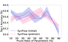
(a) SynFlow on VGG-16

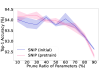
(b) SNIP on ResNet-32

Figure 9: Initialized vs. pretrained weights on CIFAR-10. Shaded regions indicate standard deviation based on three independent runs (best view in color).

Some works ([123, 167, 168, 110]) study the transferability of sparsity masks across datasets. For example, Tiwari et al. [123] compare the Top-1 accuracy of the pruned network on CIFAR-100 with the one wherein the masks are learned on Tiny ImageNet and transferred to CIFAR-100. The results show that the transferred masks perform better than those directly obtained from the original task, with 40% of the channels removed. S. Morcos et al. [109] observe that for image classification, winning tickets generated on larger datasets (such as bigger training set size and/or more number of classes) consistently transferred better than those generated with smaller datasets. For example, winning tickets generated on ImageNet and Places365 demonstrate better performance across other smaller target datasets such as CIFAR-10 and CIFAR-100. Iofinova et al. [169] present a pioneer study of the transfer performance of subnetworks and find that pruning methods with similar Top-1 accuracy on ImageNet [1] can have surprisingly different Top-1 accuracy when used for transfer learning. For architecture transfer pruning, Elastic Ticket Transformations (ETTs) [42] transforms winning tickets found in one kind of network (ResNet [6], or VGG [2]) to another deeper or shallower one from the same model family.

7.7 Static vs. Dynamic Pruning

Static pruning [12] uses static pruning criteria and permanently removes components. In contrast, dynamic pruning ([51, 136, 135, 170]) exploits input-specific characteristic pruning criteria and preserves the entire network structures and accelerates the networks by dynamically skipping unimportant components. However, dynamic pruning generally does not perform run-time fine-tuning or retraining. The difference between static and dynamic pruning is mainly reflected in the pruning criteria and the pruned model. The advantages and disadvantages of static and dynamic pruning are shown in Table IX.

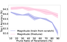
(a) Magnitude on CIFAR-10

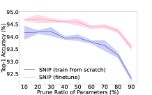
(b) SNIP on CIFAR-10

Figure 10: Training from scratch vs. fine-tuning for ResNet-32. Shaded regions indicate standard deviation based on three independent runs (best view in color).

7.8 Layer-wise Weight Density Analysis

Some works ([119, 171, 71, 154]) study the distributions of layer-wise weight density of a subnetwork, and their results show that different layers can have very different weight densities. The difference is produced by the joint action of structural characteristics of the dense network and the pruning methods. Zhang et al. [172] empirically study the heterogeneous characteristic of layers and divide the layers into either ”ambient” or ”critical”. The ambient layers are not sensitive to changing weights to the initial values, while critical layers are. It seems that the ambient layers should be pruned heavily, and the corresponding weight densities will be lower.

Pruning methods also can cause different weight densities. Take pruning for image classification as an example. Some pruning methods tend to assign more weights to earlier layers than later ones. For example, Ma et al. [119] investigate the layer-wise keep-ratios of the subnetworks obtained by GraSP, SNIP [46], LTH on VGG and ResNet, and observe the common trend of declining in layer-wise keep-ratios except for some special layers (such as the downsampling layers in ResNet). In contrast, Liu et al. [71] find their pruned networks keep higher percentages of channels in the deeper layers than those in the lower layers for image classification. The results in [171] show that global magnitude pruning tends to prune layers of Transformer uniformly [173], while global first-order methods heavily prune the deeper layers.

TABLE IX: Advantages and disadvantages of static and dynamic pruning.

Type	Advantages	Disadvantages
Static Pruning	model size reduced	fixed subnetwork
Dynamic Pruning	flexible subnetwork	model size unreduced

7.9 Pruning with Different Levels of Supervision

In descending order of supervision level during neural network pruning, pruning can be divided into supervised, semi-supervised, self-supervised, and unsupervised pruning [174]. Self-supervised learning can be divided into two classes: generative or contrastive learning [175]. Like supervised learning, supervised pruning works on fully labeled datasets. Most of the current pruning methods fall into supervised pruning. However, supervised pruning suffers from similar bottlenecks as supervised learning (such as expensive manual labeling). As a promising alternative, semi-supervised, self-supervised, and unsupervised pruning have drawn massive attention .

For example, Caron et al. [176] observe the different results in self-supervision pruning from in supervision pruning, where winning tickets initialization only introduce a slight performance improvement compared to random re-initialization. Pan et al. [177] claim that unsupervised pruning usually fails to preserve the accuracy of the original model. Notably, label supervision for network pruning and training can be independent. For example, Chen et al. [168] use supervised pruning method IMP (i.e., Iterative Magnitude Pruning) to explore the subnetworks of self-supervised pretrained models (simCLR [178] and MoCo [179]) on ImageNet. Similarly, Jeff Lai et al. [180] exploit the supervised pruning method IMP to prune self-supervised speech recognition models.

8 Fusion of Pruning and other Compression Techniques

In this section, we provide a review of the fusion of neural network pruning with other network compression techniques, such as quantization [11], tensor decomposition [144], knowledge distillation [21], and network architecture search [73]. However, on the one hand, fusion provides more choices for network compression. On the other hand, the combined compression techniques can complement each other to improve the performance and prune ratio further.

Pruning & Quantization: Quantization [147] is a compression technique to reduce the number of bits used to represent the network weights and/or activations, which can significantly reduce the model size and memory footprint but with a minor performance drop. To obtain more compacted models as well as model acceleration, Han et al. [11] pioneer to prune the redundant network connections and quantize the weights. CLIP-Q [147] jointly perform pruning and quantization during the fine-tuning stage. MPTs [108] integrates pruning and quantizing randomly weighted full-precision neural networks to obtain binary weights and/or activations. EB [130] applies 8-bit low-precision training to the stage of searching EB tickets.

Pruning & Tensor Decomposition: Tensor decomposition [19] decomposes the convolutions into a sequence of tensors with fewer parameters. In contrast to pruning, it explores the original weights’ low-rank structure, keeping the dimension of the convolutional output unchanged. CC [144] combines channel pruning and tensor decomposition to compress CNN models by simultaneously learning the model sparsity and low rankness. Hinge [181] introduces group sparsity to fuse filter pruning and decomposition under the same formulation.

Pruning & NAS: Neural Architecture Search (NAS) provides a mechanism to automatically discover the best architecture for the problem of interest, which provides a new idea for pruning to find suitable network depth and width. NPAS [73] performs a compiler-aware joint network pruning and architecture search, determining the filter type (different kernel sizes), the pruning scheme, and the rate for each layer. TAS [182] exploits NAS to search for the depth and width of a network to obtain the pruned networks and uses knowledge distillation to train these pruned networks.

Pruning & Knowledge Distillation: Knowledge Distillation (KD) [21] guides the student to effectively inherit knowledge from the teacher and mimic the output of the teacher. Some works ([183, 184]) exploit pruning before KD to boost the KD quality. For example, Liu et al. [183] prune unimportant channels to the contents of interest and focus the distillation on the interest regions. Park and No [184] prune the teacher network first to make it more transferable and then distill it to the student. Some works ([135, 185, 66]) use KD to train the pruned networks. The results in [185] show that the pruned network recovered by KD performs better than it regained by fine-tuning. Zou et al. [186] propose a data-free deraining model compression method that distills the pruned model to fit the pretrained model.

Pruning & Multi-compression Techniques: Some works ([187, 188]) explore the fusion of pruning with more than one compression technique. For example, GS [189] fuses pruning, quantization, and KD for Generative Adversarial Networks (GANs) compression. Joint-DetNAS [188] joins pruning, NAS, and KD for image translation. LadaBERT [187] integrates pruning, matrix factorization, and KD to compress Bidirectional Encoder Representations from Transformers (BERTs) [132] for natural language understanding.

9 Suggestions and Future Directions

In this section, we discuss how to choose different pruning methods and provide promising directions for future work.

9.1 Recommendations on pruning method selection

After years of research and exploration, there are many off-the-shelf pruning methods. However, no golden standard exists to measure which one is the best. Different suitable pruning methods exist to compact deep neural networks to the specific application requirements and the hardware and software resources. Here are some general recommendations for choosing an appropriate pruning method.

(1) If you do not have special hardware (e.g., FPGAs or ASICs) or software (such as sparsity convolutional libraries) but need actual neural network acceleration and compression, structured pruning is more suitable than unstructured pruning because most software frameworks and hardware cannot accelerate sparse matrices’ computation.

(2) If you have enough computational resources in the pruning stage, iterative PAT methods may be considered. Overall, this class of methods can minimize the impact on performance under the same prune ratio. On the other hand, if you have limited computational resources in both the pruning and inference stages, one-shot PBT or one-shot post-training pruning methods may be considered.

(3) If you have enough labeled examples on the target task, supervised pruning methods may be considered. However, if only a few examples on the target task are labeled, semi-supervised or transfer pruning methods may be considered. If the examples on the target task are not labeled, self-supervised, unsupervised, or transfer pruning methods may be considered.

(4) If you have enough memory footprint during pruning for NLP tasks, heavily compressing large models can be considered rather than lightly compressing smaller models to meet the same budgets. Some results in [190] show that for NLP tasks finding pruned models from large dense networks outperform small dense networks with a size comparable to pruned models.

(5) If you have enough memory footprint to store the dense neural network in the inference stage and hope to provide run-time flexible computational cost allocation for different inputs, dynamic pruning methods can be considered where inputs with smaller shapes can allocate less computational cost to perform the task and if the input shape is bigger more computational cost can be allocated.

(6) If you need to trim down neural networks in multiple dimensions, you can comprehensively consider layerwise pruning (decreasing the model’s depth), channel pruning (reducing the model’s width), and image resolution pruning (scaling down the model’s input resolution). In addition, pruning can be integrated with quantization to further reduce the memory footprint and the neural networks’ size.

(7) If you want to reach a better tradeoff between speed and accuracy, the following settings may help: use a pretrained model; set a more appropriate learning rate (if any) in both the pruning and the retraining stages; fine-tune the pruned models for several epochs; integrate pruning, knowledge distillation, NAS or other compression methods to achieve complementarity; adversarial training may have some help [111].

(8) If you need to train a subnetwork to recover loss accuracy, the results in [119] show that when residual connections exist, the subnetwork achieves higher accuracy at a relatively small learning rate. In contrast, a larger learning rate is preferable in training a subnetwork without residual connections.

9.2 Future Directions

We discuss four promising directions for the further development of neural network pruning, namely, (1) theories, (2) techniques, (3) applications, and (4) evaluation.

Theories: Despite the existing works, several fundamental questions about pruning still need to be answered. For example, prior works demonstrate that network layers contain irreplaceable information as long as redundant ones. Does a theoretical upper bound of the prune ratio exist for a given network that still keeps the matching performance of its dense equivalent? In other words, how heavily can a network be pruned theoretically without accuracy loss? It is a tricky question because of the intricate relationships between network layers. Besides, is pruning explainable? A common belief is deep neural network is hard to interpret. As such, making explainable pruning is an uphill task. However, the interpretability of pruning is vital for understanding the factors behind pruning (e.g., model structure and weights) and exploring more effective pruning methods.

Techniques: To obtain better algorithm designs whose architectures are learned in an economical, efficient, and effective manner, it is a trend to extend Automated Machine Learning (AutoML) methods and NAS to pruning. Furthermore, pruning also begins to combine with various learning contexts, such as lifelong learning [66], continual learning [191], contrast learning [32], federated learning [192], etc. In addition, networks’ rising energy consumption requires more attention to energy-aware pruning. However, preliminary efforts mainly focus on reducing computation and memory costs, which may not necessarily reduces the most energy consumption. Besides, incorporating pruning into the hardware to help deploy pruned networks is also an emerging trend. For example, Sui et al. [54] propose a hardware-friendly pruning method and deploy the pruned models on the FPGA platform.

Applications: The prior mainstream research targets pruning studies in CV, especially in image classification. Recently, pruning has begun to draw attention to more complex applications, like object tracking, visual question answering, natural language understanding, speech recognition, etc. For example, in recent years, foundation models such as GPT-4 [193] might be the possible way to Artificial General Intelligence (AGI). However, its huge model hinders its application in many downstream tasks. Therefore, colossal foundation models can benefit from pruning research to be more compact and efficient [15].

Evaluation: With the emergence of many pruning methods, standardized benchmarks and metrics are required to provide a fair evaluation. Different pruning techniques, network architectures, tasks, and experimental settings lead to incomparable results and make it hard to compare pruning methods fairly [194]. ShrinkBench [37] takes the first step and provides a benchmark of pruning methods for image classification. As pruning is applied to applications other than image classification, standardized benchmarks and metrics for other applications are needed.

10 Conclusion

As an essential compression technique, deep neural network pruning has attracted increasing research attention with the recent emergence of a wide variety of pruning methods and applications. This survey conducts a comprehensive review on the following four scopes: 1) universal/specific speedup, with a systematic review from unstructured, structured, and semi-structured pruning; 2) when to prune, including pruning before/during/after training for static pruning and run-time pruning; 3) how to prune, including pruning by heuristic criteria and by learning; 4) fusion of pruning with other compression techniques, such as KD, NAS, so on. A comprehensive comparative analysis, including seven pairs of contrast settings for pruning, layer-wise weight density, and different supervision levels, can help researchers to efficiently and effectively grasp the characteristics of different pruning methods. Additionally, recommendations on pruning method selection and future research directions are highlighted and discussed. To facilitate future research, real-world miscellaneous applications and commonly used resources of datasets, networks, and evaluation metrics in different applications are summarized in Appedix B. To help researchers and practitioners keep up with the development of pruning technologies, we continue updating the representative research efforts and open-source codes for pruning at https://github.com/hrcheng1066/awesome-pruning.

Appendix A Experimental settings

In the main work, we use CIFAR-10 [156] and CIFAR-100 [156] to evaluate the pruning methods on both VGGNet [2] and ResNet [6]. CIFAR-10 and CIFAR-100 datasets contain 50K training and 10K test images for 10 and 100 classes, respectively. We adopt SGD as an optimizer with momentum [195] of 0.9, weight decay of $10^{-4}$, train the networks for 160 epochs by using batch size 128 with an initial learning rate of 0.1, and reduce the learning rate at epochs 60 and 120, as used in [39]. The code for SNIP and GraSP is available at https://github.com/JingtongSu/sanity-checking-pruning. The code for SynFlow is available at https://github.com/ganguli-lab/Synaptic-Flow.

Appendix B Pruning for Specific Applications

This section summarizes the mainstream applications’ characteristics involved in pruning, and the commonly used networks, datasets, and evaluation metrics of pruning are shown in Table X. The statistics of pruning literature in different applications are shown in Fig. 12(a).

B.1 Image Classification

Image classification refers to classifying images according to their visual content and is the most basic task for pruning. Since image classification mainly relies on CNNs, the corresponding study (such as [71, 50, 47, 46]) mainly focuses on pruning CNNs. Only a few works ([196]) propose pruning methods for other kinds of neural networks, such as vision transformers. Most pruning works provide experimental results on ImageNet [1]. The representative pruning results on ImageNet refer to Supplementary.

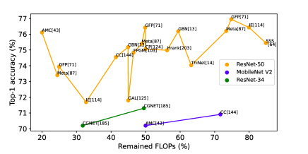
Figure 11: Top-1 accuracy of representative pruning methods on ImageNet (best view in color and zoom in).

The representative pruning results on ImageNet are shown in Fig. 11, where the results are taken directly from the corresponding papers. The networks used in papers with the same name may differ in the network structures, leading to different accuracy even if the other settings are the same. For example, some works ([50, 60]) expand the layers’ width of ResNet-32 by a factor (such as 2 or 4). The Top-1 accuracy of the expanded ResNet-32 is higher than vanilla ResNet-32. Some works ([62, 64]) use VGG-16 with one FC layer, while others ([125, 85]) adopt two or three FC layers.

B.2 Object Detection

In comparison with image classification, object detection requires predicting the class and the exact location of each object in an image. Correspondingly, the neural networks for object detection have more complex architectures, including backbones and other detection parts. In addition, object detection generally requires larger input sizes. These make pruning for object detection more challenging than image classification. Only a few works ([188, 197]) study pruning for object detection. For instance, Bonnaerens et al. [197] propose an anchor pruning method. Girish et al. [198] investigate LTH for object detection. GFP [71] prunes one-stage and two-stage object detection models to validate performance.

As shown in Table X, the accuracy metrics include mAP (mean Average Precision) and the COCO mAP that is the mAP evaluated at Intersection-Over-Union (IoU) thresholds evenly distributed between 0.5 and 0.95.

B.3 Image Style Translation

Image style translation which means transferring style from one image to another is an important application for deploying GANs on mobile devices. Compared with the networks for image classification, GANs have very different network structures and outputs, which consist of a generator and a discriminator and output high-dimension images. Shu et al. [199] find two major differences between compressing models for image classification and GANs. First, the discriminator network does not need to be compact because it will be discarded after training the generative network. Second, it is difficult to quantitatively evaluate the output images by GANs. Besides, the training difficulty causes extra challenges for pruning GANs [199]. Some pruning methods ([199, 189]) are proposed to reduce GAN’s parameters and computational complexities. For example, Chen et al. [200] prune CycleGAN to verify matching subnetworks in GANs.

As shown in Table X, FCN-scores [201], and Fréchet Inception Distance (FID) are often utilized to evaluate the pruning results. FCN-scores include pixel accuracy, class accuracy, and class IoU. The larger FID is, the better the transfer results are.

B.4 Adversarial Robustness

In safety-critical but computationally resource-constrained applications, neural network pruning faces another challenge whether the sparse models can preserve robustness. While the research community has extensively explored robust training and network pruning independently, only a few recent works ([141, 16]) have studied them jointly. For example, Sehwag et al. [141] empirically verify that adversarial robustness can be achieved with weight magnitude-based pruning heuristic. HYDRA [16] increases the awareness of pruning techniques to the robust training objective and formulates the pruning objective as an empirical risk minimization problem.

As shown in Table X, the benign accuracy refers to the percentage of correctly classified original (i.e., non-modified) inputs. Empirical Robust Accuracy (ERA) refers to the percentage of robust test samples under gradient-based attacks. Verifiable Robust Accuracy (VRA) corresponds to the fraction of test samples that are verified to be robust by network verification methods in [202].

TABLE X: Summary of commonly used pruning evaluation for various applications. The first five rows belong to CV tasks, the last row belongs to speech processing tasks, and the other rows belong to NLP tasks.

Task	Dataset	Model	Performance	Efficiency	Example work
Image	CIFAR-10/100 [156],	ResNet-32/50/56 [6],	Top-1/Top-5 accuracy	FLOPs,	[47], [203],
Classification	ImageNet ILSVRC2012 [1]	VGG-16/19 [2],		MACs,	[50], [71],
		MobileNet V1/V2 [204]		$\lVert\mathbf{w}\rVert_{0}$	[102], [39]
Object	MS COCO [3],	RetinaNet [205],	mAP,	FLOPs,	[71], [197],
Detection	PASCAL VOC 2007/2010 [206],	Faster R-CNN [207],	COCO mAP	$\lVert\mathbf{w}\rVert_{0}$	[198]
		SSD [208]
Image Style	horse2zebra [209],	CycleGAN [209]	FCN-scores [201],	FLOPs,	[199], [189]
Translation	summer2winter [209],		FID [210]	$\lVert\mathbf{w}\rVert_{0}$
	Cityscapes [211]
Adversarial	CIFAR-10 [156],	VGG-16 [2],	Top-1/Top-5 accuracy,	$\lVert\mathbf{w}\rVert_{0}$	[16]
Robustness	ImageNet ILSVRC2012 [1]	ResNet-18/50 [6],	benign accuracy,
		Wide-ResNet-28-5	ERA/VRA [141]
Human-pose	MS COCO [3]	CMU-pose [212]	mAP		[45]
Estimation
Machine	WMT’14/16,	Transformer-based [173],	BLEU [213],	FLOPs,	[214], [139],
Translation	OpenSubtitles2018 [215]	LSTMs [216]		$\lVert\mathbf{w}\rVert_{0}$	[217], [153]
Natural Language	GLUE [218],	BERT [4]	accuracy,	$\lVert\mathbf{w}\rVert_{0}$	[167], [171],
Understanding	SQuAD [219],		Pearson/Matthew cor.,		[131]
	MultiNLI [220]		F1
Language	Wikitext-2 [221],	LSTMs [216]	Perplexity	$\lVert\mathbf{w}\rVert_{0}$	[214], [217]
Modeling	Penn Tree Bank [222]
Speech Recognition	TED-LIUM [223],	wav2vec 2.0 [224],	WER,	$\lVert\mathbf{w}\rVert_{0}$	[145], [225],
	Common Voice [226],	LSTMs [216],	CER		[180]
	LibriSpeech [227]	Conformer [228]

B.5 Other CV Tasks

In addition to the above CV tasks, some works explore pruning methods for other CV tasks, such as semantic segmentation ([198]), image deraining ([186]), human-pose estimation ([45]), head-pose estimation ([229]), image super-resolution ([152]), object tracking [230], and backdoor attack [231] etc. For example, Wang et al. [45] prune CMU-pose model [212] for human pose estimation. Li et al. [152] prune DnCNN [232] and U-Net [233] for image denoising.

(a) Pipelines & applications

B.6 Natural Language Processing

Long Short-Term Memory (LSTM) [216], transformer [173], and transformer-based networks (such as BERT [4]) have become the dominant modeling paradigm in natural language processing. In contrast to CNNs, RNNs [234] based networks reuse activation functions to produce sequence output. To lower computational cost and obtain acceleration, a few works ([139, 214, 217, 153]) explore network pruning for NLP. See et al. [139] explore one of the earliest pruning methods of deep neural networks for NLP, where the magnitude-based method is proposed to prune LSTM for machine translation. Yu et al. [214] explore the lottery hypothesis in NLP. Voita et al. [153] prune multi-head self-attention of Transformer [173]. Chen et al. [167] pioneer to study the lottery ticket hypothesis in pretrained BERT [4] models and find matching subnetworks. EarlyBERT [131]) find structured winning tickets in the early stage of BERT training. Gan et al. [111] investigate lottery ticket in vision-and-language tasks and find “relaxed” winning tickets that match 99% of the full accuracy can be found with 50%-70% prune ratio of parameters in UNITER [235].

As shown in Table X , the GLUE benchmark provides nine tasks and their corresponding metrics, including accuracy, Pearson correlation, Matthew’s correlation, etc. BiLingual Evaluation Understudy (BLEU) score [213] is often used for evaluating the accuracy of machine translation. Perplexity is used for language modeling or machine translation to measure the pruning change in performance. The lower the Perplexity, the better the pruned model.

B.7 Audio and Speech Processing

Speech recognition is one of the most common audio and speech processing. Lightweight speech recognition has become an indispensable feature on mobile devices. Nrang et al. [145] prune Deep Speech 2 [236], a recurrent neural network architecture, to validate their gradual pruning scheme. Ding et al. [225] extend the lottery ticket hypothesis to speech recognition models and investigate the existence of winning tickets. PARP [180] prunes pretrained wav2vec 2.0 [224] and XLSR-53 [237] for self-supervised speech recognition.

As shown in Table X, the Word Error Rate (WER) is the standard metric measuring the accuracy of speech recognition, which is defined as $\textrm{WER}=(S+I+D)/(S+I+C)$, where $S$, $I$, $D$ and $C$ denote the number of substitutions, insertions, deletions, and correct words, respectively. The lower the value, the better the accuracy of the speech recognition model. The Character Error Rate (CER) has the exact definition of WER, except that CER counts characters while WER counts words.

References

- Russakovsky et al. [2015] O. Russakovsky, J. Deng, H. Su, J. Krause, S. Satheesh, S. ma, Z. Huang, A. Karpathy, A. Khosla, M. Bernstein, A. C. Berg, and F. fei Li, “ImageNet large scale visual recognition challenge,” IJCV, vol. 115, pp. 211–252, 2015.
- Simonyan and Zisserman [2015] K. Simonyan and A. Zisserman, “Very deep convolutional networks for large-scale image recognition,” in ICLR, 2015.
- Lin et al. [2014] T.-Y. Lin, M. Maire, S. Belongie, J. Hays, P. Perona, D. Ramanan, P. Dollar, and L. Zitnick, “Microsoft COCO: Common objects in context,” in ECCV, 2014.
- Devlin et al. [2019] J. Devlin, M.-W. Chang, K. Lee, and K. Toutanova, “BERT: Pre-training of deep bidirectional transformers for language understanding,” in NAACL, 2019.
- Bohnstingl et al. [2021] T. Bohnstingl, A. Garg, S. Woźniak, G. Saon, E. Eleftheriou, and A. Pantazi, “Towards efficient end-to-end speech recognition with biologically-inspired neural networks,” in NeurIPS, 2021.
- He et al. [2016] K. He, X. Zhang, S. Ren, , and J. Sun, “Deep residual learning for image recognition,” in CVPR, 2016, pp. 770–778.
- You et al. [2020a] H. You, C. Li, P. Xu, Y. Fu, Y. Wang, X. Chen, R. G. Baraniuk, Z. Wang, and Y. Lin, “Drawing early-bird tickets: Towards more efficient training of deep networks,” in ICLR, 2020.
- Choudhary et al. [2020] T. Choudhary, V. Mishra, A. Goswami, and J. Sarangapani, “A comprehensive survey on model compression and acceleration,” Artificial Intelligence Review, pp. 5113–5155, 2020.
- Wu et al. [2023] J. Wu, W. Gan, Z. Chen, S. Wan, and H. Lin, “AI-generated content AIGC: A survey,” 2023. [Online]. Available: http://arxiv.org/abs/2303.04226
- Han et al. [2015] S. Han, J. Pool, J. Tran, and W. Dally, “Learning both weights and connections for efficient neural network,” in NIPS, vol. 1, 2015.
- Han et al. [2016a] S. Han, H. Mao, and W. J. Dally, “Deep compression: Compressing deep neural networks with pruning, trained quantization and huffman coding,” in ICLR, 2016.
- Dong et al. [2017] X. Dong, J. Huang, Y. Yang, and S. Yan, “More is Less: A more complicated network with less inference complexity,” in CVPR, 2017.
- You et al. [2019] Z. You, K. Yan, J. Ye, M. Ma, and P. Wang, “Gate Decorator: Global filter pruning method for accelerating deep convolutional neural networks,” in NeurIPS, 2019.
- Luo et al. [2017] J.-H. Luo, J. Wu, and W. Lin, “ThiNet: A filter level pruning method for deep neural network compression,” in ICCV, 2017.
- Frantar and Alistarh [2023] E. Frantar and D. Alistarh, “SparseGPT: Massive language models can be accurately pruned in one-shot,” 2023. [Online]. Available: https://arxiv.org/pdf/2301.00774.pdf
- Sehwag et al. [2020] V. Sehwag, S. Wang, P. Mittal, and S. Jana, “HYDRA: Pruning adversarially robust neural networks,” in NeurIPS, 2020.
- Chen and Zhao [2019] S. Chen and Q. Zhao, “Shallowing deep networks: Layer-wise pruning based on feature representations,” TPAMI, vol. 41, no. 12, pp. 3048–3056, 2019.
- Denton et al. [2014] E. Denton, W. Zaremba, J. Bruna, Y. LeCun, and R. Fergus, “Exploiting linear structure within convolutional networks for efficient evaluation,” in NIPS, vol. 1, 2014, pp. 1269–1277.
- Lin et al. [2018] S. Lin, R. Ji, C. Chen, D. Tao, and J. Luo, “Holistic CNN compression via low-rank decomposition with knowledge transfer,” TPAMI, 2018.
- Banner et al. [2019] R. Banner, Y. Nahshan, and D. Soudry, “Post training 4-bit quantization of convolutional networks for rapid-deployment,” in NeurIPS, 2019, pp. 7950–7958.
- Hinton et al. [2015] G. Hinton, O. Vinyals, and J. Dean, “Distilling the knowledge in a neural network,” 2015. [Online]. Available: http://arxiv.org/abs/1503.02531
- Liu et al. [2019a] H. Liu, K. Simonyan, and Y. Yang, “DARTS: Differentiable architecture search,” in ICLR, 2019.
- Zhang et al. [2021a] M. Zhang, S. Su, S. Pan, X. Chang, E. Abbasnejad, and R. Haffari, “iDARTS: Differentiable architecture search with stochastic implicit gradients,” in ICML, 2021.
- Fu et al. [2022] Y. Fu, H. Yang, J. Yuan, M. Li, C. Wan, R. Krishnamoorthi, V. Chandra, and Y. Lin, “Depthshrinker: a new compression paradigm towards boosting real-hardware efficiency of compact neural networks,” in ICML, 2022.
- Ding et al. [2021] X. Ding, X. Zhang, N. Ma, J. Han, G. Ding, and J. Sun, “RepVGG: making VGG-style ConvNets great again,” in CVPR, 2021.
- Hanson and Pratt [1988] S. Hanson and L. Pratt, “Comparing biases for minimal network construction with back-propagation,” in NIPS, vol. 1, 1988.
- Mishra et al. [2020] R. Mishra, H. Prabhat Gupta, and T. Dutta, “A survey on deep neural network compression: Challenges, overview, and solutions,” 2020. [Online]. Available: https://arxiv.org/pdf/2010.03954.pdf
- T. O’ Neill [2020] J. T. O’ Neill, “An survey of neural network compression,” 2020. [Online]. Available: https://arxiv.org/pdf/2006.03669.pdf
- Ghimire et al. [2022] D. Ghimire, D. Kil, and S. heum Kim, “A survey on efficient convolutional neural networks and hardware acceleration,” Electronics, vol. 11, no. 945, 2022.
- Liu et al. [2020a] J. Liu, S. Tripathi, U. Kurup, and M. Shah, “Pruning algorithms to accelerate convolutional neural networks for edge applications: A survey,” 2020. [Online]. Available: https://arxiv.org/pdf/2005.04275.pdf
- Hoefler et al. [2021] T. Hoefler, D. Alistarh, T. Ben-Nun, N. Dryden, and A. Peste, “Sparsity in deep learning: pruning and growth for efficient inference and training in neural networks,” JMLR, vol. 22, no. 241, pp. 1–124, 2021.
- Corti et al. [2022] F. Corti, R. Entezari, S. Hooker, D. Bacciu, and O. Saukh, “Studying the impact of magnitude pruning on contrastive learning methods,” in ICML, 2022.
- Elkerdawy et al. [2022] S. Elkerdawy, M. Elhoushi, H. Zhang, and N. Ray, “Fire together wire together: A dynamic pruning approach with self-supervised mask prediction,” in CVPR, 2022, pp. 12 454–12 463.
- Wang et al. [2022] H. Wang, C. Qin, Y. Bai, Y. Zhang, and Y. Fu, “Recent advances on neural network pruning at initialization,” in IJCAI, 2022.
- He and Xiao [2023] Y. He and L. Xiao, “Structured pruning for deep convolutional neural networks: A survey,” 2023. [Online]. Available: https://arxiv.org/pdf/2303.00566.pdf
- Reed [1993] R. Reed, “Pruning algorithms-a survey,” IEEE Transactions on Neural Networks, vol. 4, no. 5, pp. 740–747, 1993.
- Blalock et al. [2020] D. Blalock, J. J. G. Ortiz, J. Frankle, and J. Guttag, “What is the state of neural network pruning?” in MLSys, 2020.
- Liu et al. [2019b] Z. Liu, M. Sun, T. Zhou, G. Huang, and T. Darrell, “Rethinking the value of network pruning,” in ICLR, 2019.
- Tanaka et al. [2020] H. Tanaka, D. Kunin, D. L. Yamins, and S. Ganguli, “Pruning neural networks without any data by iteratively conserving synaptic flow,” in NeurIPS, vol. 33, 2020, pp. 6377–6389.
- Renda et al. [2020] A. Renda, J. Frankle, and M. Carbin, “Comparing rewinding and fine-tuning in neural network pruning,” in ICLR, 2020.
- Qian and Klabjan [2021] X. Qian and D. Klabjan, “A probabilistic approach to neural network pruning,” in ICML, 2021.
- Chen et al. [2021a] X. Chen, Y. Cheng, S. Wang, Z. Gan, J. Liu, and Z. Wang, “The elastic lottery ticket hypothesis,” in NeurIPS, 2021.
- He et al. [2018a] Y. He, J. Lin, Z. Liu, H. Wang, L.-J. Li, and S. Han, “AMC: AutoML for model compression and acceleration on mobile devices,” in ECCV, 2018, pp. 784–800.
- Fang et al. [2023] G. Fang, X. Ma, M. Song, M. B. Mi, and X. Wang, “DepGraph: Towards any structural pruning,” in CVPR, 2023.
- Wang et al. [2018] D. Wang, L. Zhou, X. Zhang, X. Bai, and J. Zhou, “Exploring linear relationship in feature map subspace for ConvNets compression,” 2018. [Online]. Available: http://arxiv.org/abs/1803.05729
- Lee et al. [2019] N. Lee, T. Ajanthan, and P. H. Torr, “SNIP: Single-shot network pruning based on connection sensitivity,” in ICLR, 2019.
- Frankle and Carbin [2019] J. Frankle and M. Carbin, “The lottery ticket hypothesis: finding sparse, trainable neural networks,” in ICLR, 2019.
- Frankle et al. [2021] J. Frankle, G. K. Dziugaite, D. M. Roy, and M. Carbin, “Pruning neural networks at initialization: why are we missing the mark?” in ICLR, 2021.
- He et al. [2020] Y. He, Y. Ding, P. Liu, L. Zhu, H. Zhang, and Y. Yang, “Learning filter pruning criteria for deep convolutional neural networks acceleration,” in CVPR, 2020, pp. 2009–2018.
- Nonnenmacher et al. [2022] M. Nonnenmacher, T. Pfeil, I. Steinwart, and D. Reeb, “SOSP: Efficiently capturing global correlations by second-order structured pruning,” in ICLR, 2022.
- Tang et al. [2021] Y. Tang, Y. Wang, Y. Deng, C. Xu, D. Tao, and C. Xu, “Manifold regularized dynamic network pruning,” in CVPR, 2021.
- Hayou et al. [2021] S. Hayou, J.-F. Ton, A. Doucet, and Y. W. Teh, “Robust pruning at initialization,” in ICLR, 2021.
- Frankle et al. [2020] J. Frankle, G. K. Dziugaite, D. M. Roy, and M. Carbin, “Linear mode connectivity and the lottery ticket hypothesis,” in ICML, 2020.
- Sui et al. [2023] X. Sui, Q. Lv, L. Zhi, B. Zhu, Y. Yang, Y. Zhang, and Z. Tan, “A hardware-friendly high-precision cnn pruning method and its fpga implementation,” Sensors, vol. 23, 2023.
- Ma et al. [2020a] X. Ma, F. Guo, W. Niu, X. Lin, J. Tang, K. Ma, B. Ren, and Y. Wang, “PCONV: The missing but desirable sparsity in DNN weight pruning for real-time execution on mobile devices,” in AAAI, 2020.
- Ma et al. [2020b] X. Ma, W. Niu, T. Zhang, S. Liu, S. Lin, H. Li, W. Wen, X. Chen, J. Tang, K. Ma, B. Ren, and Y. Wang, “An image enhancing pattern-based sparsity for real-time inference on mobile devices,” in ECCV, 2020.
- Wang et al. [2019a] Z. Wang, J. Wohlwend, and T. Lei, “Structured pruning of large language models,” 2019. [Online]. Available: https://arxiv.org/abs/1910.04732
- Wang and Fu [2023] H. Wang and Y. Fu, “Trainability preserving neural structured pruning,” in ICLR, 2023.
- Wolfe and Kyrillidis [2022] C. R. Wolfe and A. Kyrillidis, “i-SpaSP: Structured neural pruning via sparse signal recovery,” in PMLR, vol. 168, 2022.
- Su et al. [2020] J. Su, Y. Chen, T. Cai, T. Wu, R. Gao, L. Wang, and J. D. Lee, “Sanity-checking pruning methods: random tickets can win the jackpot,” in NeurIPS, vol. 33, 2020, pp. 20 390–20 401.
- Wang et al. [2020a] C. Wang, G. Zhang, and R. Grosse, “Picking winning tickets before training by preserving gradient flow,” in ICLR, 2020.
- Liu et al. [2017] Z. Liu, J. Li, Z. Shen, G. Huang, Shoumeng, and Z. Changshui, “Learning efficient convolutional networks through network slimming,” in ICCV, 2017, pp. 2736–2744.
- Wen et al. [2016] W. Wen, C. Wu, Y. Wang, Y. Chen, and H. Li, “Learning structured sparsity in deep neural networks,” in NIPS, 2016.
- Huang and Wang [2018] Z. Huang and N. Wang, “Data-driven sparse structure selection for deep neural networks,” in ECCV, 2018, pp. 304–320.
- Bai et al. [2022] Y. Bai, H. Wang, Z. Tao, K. Li, and Y. Fu, “Dual lottery ticket hypothesis,” in ICLR, 2022.
- Chen et al. [2021b] T. Chen, Z. Zhang, S. Liu, S. Chang, and Z. Wang, “Long live the lottery: the existence of winning tickets in lifelong learning,” in ICLR, 2021.
- Chen et al. [2021c] T. Chen, Y. Sui, X. Chen, A. Zhang, and Z. Wang, “A unified lottery ticket hypothesis for graph neural networks,” in ICML, 2021.
- Liu et al. [2020b] J. Liu, Z. Xu, R. Shi, R. C. Cheung, and H. K. So, “Dynamic sparse training: Find efficient sparse network from scratch with trainable masked layers,” in ICLR, 2020.
- Li et al. [2017] H. Li, A. Kadav, I. Durdanovic, H. Samet, and H. P. Graf, “Pruning filters for efficient convnets,” in ICLR, 2017.
- Han et al. [2016b] S. Han, X. Liu, H. Mao, J. Pu, A. Pedram, M. A. Horowitz, and W. J. Dally, “EIE: Efficient inference engine on compressed deep neural network,” in ISCA, 2016.
- Liu et al. [2021a] L. Liu, S. Zhang, Z. Kuang, A. Zhou, J.-H. Xue, X. Wang, Y. Chen, W. Yang, Q. Liao, and W. Zhang, “Group fisher pruning for practical network compression,” in ICML, 2021.
- Ding et al. [2019a] X. Ding, G. Ding, Y. Guo, J. Han, and C. Yan, “Approximated oracle filter pruning for destructive CNN width optimization,” in ICML, 2019.
- Li et al. [2021a] Z. Li, G. Yuan, W. Niu, P. Zhao, Y. Li, Y. Cai, X. Shen, Z. Zhan, Z. Kong, Q. Jin, Z. Chen, S. Liu, K. Yang, B. Ren, Y. Wang, and X. Lin, “NPAS: A compiler-aware framework of unified network pruning and architecture search for beyond real-time mobile acceleration,” in CVPR, 2021, pp. 14 255–14 266.
- Meng et al. [2020] F. Meng, H. Cheng, K. Li, H. Luo, X. Guo, G. Lu, and X. Sun, “Pruning filter in filter,” in NeurIPSW, 2020.
- Liu et al. [2022a] S. Liu, T. Chen, X. Chen, L. Shen, D. C. Mocanu, Z. Wang, and M. Pechenizkiy, “The unreasonable effectiveness of random pruning: Return of the most naive baseline for sparse training,” in ICLR, 2022.
- Wang et al. [2020b] Y. Wang, X. Zhang, L. Xie, J. Zhou, H. Su, B. Zhang, and X. Hu, “Pruning from scratch,” in AAAI, 2020, pp. 12 273–12 280.
- Lee et al. [2020] N. Lee, T. Ajanthan, S. Gould, and P. H. Torr, “A signal propagation perspective for pruning neural networks at initialization,” in ICLR, 2020.
- Saxe et al. [2014] A. M. Saxe, J. L. McClelland, and S. Ganguli, “Exact solutions to the nonlinear dynamics of learning in deep linear neural networks,” in ICLR, 2014.
- Gebhart et al. [2021] T. Gebhart, U. Saxena, and P. Schrater, “A unified paths perspective for pruning at initialization,” 2021. [Online]. Available: https://arxiv.org/pdf/2101.10552.pdf
- Jacot et al. [2018] A. Jacot, F. Gabriel, and C. Hongler, “Neural tangent kernel: Convergence and generalization in neural networks,” in NIPS, 2018.
- Zhou et al. [2019] H. Zhou, J. Lan, R. Liu, and J. Yosinski, “Deconstructing lottery tickets: Zeros, signs, and the supermask,” in NeurIPS, 2019.
- Gaier and Ha [2019] A. Gaier and D. Ha, “Weight agnostic neural networks,” in NeurIPS, 2019.
- Ramanujan et al. [2020] V. Ramanujan, M. Wortsman, A. Kembhavi, A. Farhadi, and M. Rastegari, “What’s hidden in a randomly weighted neural network?” in CVPR, 2020.
- Evci et al. [2020] U. Evci, T. Gale, J. Menick, P. S. Castro, and E. Elsen, “Rigging the lottery: Making all tickets winners,” in ICML, 2020.
- Zhao et al. [2019] C. Zhao, B. Ni, J. Zhang, Q. Zhao, W. Zhang, and Q. Tian, “Variational convolutional neural network pruning,” in CVPR, 2019, pp. 2780–2789.
- He et al. [2018b] Y. He, G. Kang, X. Dong, Y. Fu, and Y. Yang, “Soft filter pruning for accelerating deep convolutional neural networks,” in IJCAI, 2018, pp. 2234–2240.
- Liu et al. [2019c] Z. Liu, H. Mu, X. Zhang, Z. Guo, X. Yang, T. K.-T. Cheng, and J. Sun, “Metapruning: Meta learning for automatic neural network channel pruning,” in ICCV, 2019, pp. 3295–3304.
- Ding et al. [2019b] X. Ding, G. Ding, X. Zhou, Y. Guo, J. Han, and J. Liu, “Global sparse momentum SGD for pruning very deep neural networks,” in NeurIPS, 2019, pp. 6379–6391.
- Yuan and Lin [2006] M. Yuan and Y. Lin, “Model selection and estimation in regression with grouped variables,” Journal of the Royal Statistical Society: Series B (Statistical Methodology), vol. 68, pp. 49–67, 2006.
- Gordon et al. [2018] A. Gordon, E. Eban, O. Nachum, and B. Chen, “MorphNet:fast & simple resource-constrained structure learning of deep networks,” in CVPR, 2018.
- Li et al. [2019a] T. Li, B. Wu, Y. Yang, Y. Fan, Y. Zhang, and W. Liu, “Compressing convolutional neural networks via factorized convolutional filters,” in CVPR, 2019, pp. 3977–3986.
- Boyd et al. [2010] S. Boyd, N. Parikh, E. Chu, B. Peleato, and J. Eckstein, “Distributed optimization and statistical learning via the alternating direction method of multipliers,” Foundations and Trends in Machine Learning, vol. 3, no. 1, pp. 1–122, 2010.
- Mocanu et al. [2018] D. C. Mocanu, E. Mocanu, P. Stone, P. H. Nguyen, M. Gibescu, and A. Liotta, “Scalable training of artificial neural networks with adaptive sparse connectivity inspired by network science,” Nature Communications, vol. 9, no. 1, 2018.
- Dai et al. [2019] X. Dai, H. Yin, and N. K. Jha, “NeST: A neural network synthesis tool based on a grow-and-prune paradigm,” IEEE Transactions on Computers, vol. 68, pp. 1487–1497, 2019.
- Mostafa and Wang [2019] H. Mostafa and X. Wang, “Parameter efficient training of deep convolutional neural networks by dynamic sparse reparameterization,” in ICML, 2019.
- Liu et al. [2021b] S. Liu, T. Chen, X. Chen, Z. Atashgahi, L. Yin, H. Kou, L. Shen, M. Pechenizkiy, Z. Wang, and D. C. Mocanu, “Sparse training via boosting pruning plasticity with neuroregeneration,” in NeurIPS, 2021.
- Lin et al. [2020a] T. Lin, S. U. Stich, L. Barba, D. Dmitriev, and M. Jaggi, “Dynamic model pruning with feedback,” in ICLR, 2020.
- Dettmers and Zettlemoyer [2019] T. Dettmers and L. Zettlemoyer, “Sparse networks from scratch: Faster training without losing performance,” 2019. [Online]. Available: https://arxiv.org/abs/1907.04840
- Liu et al. [2022b] S. Liu, T. Chen, Z. Atashgahi, X. Chen, G. Sokar, E. Mocanu, M. Pechenizkiy, Z. Wang, and D. C. Mocanu, “Deep ensembling with no overhead for either training or testing: The all-round blessings of dynamic sparsity,” in ICLR, 2022.
- Sokar et al. [2022] G. Sokar, E. Mocanu, D. C. Mocanu, M. Pechenizkiy, and P. Stone, “Dynamic sparse training for deep reinforcement learning,” in IJCAI, 2022.
- Graesser et al. [2022] L. Graesser, U. Evci, E. Elsen, and P. S. Castro, “The state of sparse training in deep reinforcement learning,” in ICML, 2022.
- Evci et al. [2022] U. Evci, Y. A. Ioannou, C. Keskin, and Y. Dauphin, “Gradient flow in sparse neural networks and how lottery tickets win,” in AAAI, 2022.
- He et al. [2019] Y. He, P. Liu, Z. Wang, Z. Hu, and Y. Yang, “Filter pruning via geometric median for deep convolutional neural networks acceleration,” in CVPR, 2019, pp. 4340–4349.
- Fletcher et al. [2008] P. Fletcher, S. Venkatasubramanian, and S. Joshi, “Robust statistics on riemannian manifolds via the geometric median,” in CVPR, 2008.
- Ioffe and Szegedy [2015] S. Ioffe and C. Szegedy, “Batch Normalization: Accelerating deep network training by reducing internal covariate shift,” 2015. [Online]. Available: https://arxiv.org/abs/1502.03167
- Malach et al. [2020] E. Malach, G. Yehudai, S. Shalev-Shwartz, and O. Shamir, “Proving the lottery ticket hypothesis: Pruning is all you need,” in ICML, 2020.
- Orseau et al. [2020] L. Orseau, M. Hutter, and O. Rivasolata, “Logarithmic pruning is all you need,” in NeurIPS, 2020.
- Diffenderfer and Kailkhura [2021] J. Diffenderfer and B. Kailkhura, “Multi-prize lottery ticket hypothesis: finding a accurate binary neural networks by pruning a randomly weighted network,” in ICLR, 2021.
- S. Morcos et al. [2019] A. S. Morcos, H. Yu, M. Paganini, and Y. Tian, “One ticket to win them all: Generalizing lottery ticket initializations across datasets and optimizers,” in NeurIPS, 2019.
- Mehta [2019] R. Mehta, “Sparse transfer learning via winning lottery tickets,” 2019. [Online]. Available: https://arxiv.org/abs/1905.07785
- Gan et al. [2022] Z. Gan, Y.-C. Chen, L. Li, T. Chen, Y. Cheng, S. Wang, J. Liu, L. Wang, and Z. Liu, “Playing lottery tickets with vision and language,” in AAAI, 2022.
- Zhou et al. [2020] J. Zhou, G. Cui, Z. Zhang, C. Yang, Z. Liu, and M. Sun, “Graph neural networks: A review of methods and applications,” AI Open, pp. 57–81, 2020.
- Ding et al. [2018] X. Ding, G. Ding, J. Han, and S. Tang, “Auto-balanced filter pruning for efficient convolutional neural networks,” in AAAI, vol. 32, no. 1, 2018.
- Molchanov et al. [2019] P. Molchanov, A. Mallya, S. Tyree, I. Frosio, and J. Kautz, “Importance estimation for neural network pruning,” in CVPR, 2019.
- Lin et al. [2019a] S. Lin, R. Ji, Y. Li, C. Deng, and X. Li, “Towards compact ConvNets via structure-sparsity regularized filter pruning,” TNNLS, 2019.
- Wang et al. [2021] H. Wang, C. Qin, Y. Zhang, and Y. Fu, “Neural pruning via growing regularization,” in ICLR, 2021.
- Zhang et al. [2021b] Z. Zhang, J. Jin, Z. Zhang, Y. Zhou, X. Zhao, J. Ren, J. Liu, L. Wu, R. Jin, and D. Dou, “Validating the lottery ticket hyphothesis with inertial manifold theory,” in NeurIPS, 2021.
- Zhang et al. [2021c] S. Zhang, M. Wang, S. Liu, P.-Y. Chen, and J. Xiong, “Why lottery ticket wins? a theoretical perspective of sample complexity on pruned neural networks,” in NeurIPS, 2021.
- Ma et al. [2021] X. Ma, G. Yuan, X. Shen, T. Chen, X. Chen, X. Chen, N. Liu, M. Qin, S. Liu, Z. Wang, and Y. Wang, “Sanity checks for lottery tickets: Does your winning ticket really win the jackpot?” in NeurIPS, 2021.
- Liu et al. [2021c] N. Liu, G. Yuan, Z. Che, X. Shen, X. Ma, Q. Jin, J. Ren, J. Tang, S. Liu, and Y. Wang, “Lottery ticket preserves weight correlation: Is it desirable or not?” in ICML, 2021.
- Zhuang et al. [2018] Z. Zhuang, M. Tan, B. Zhuang, J. Liu, Y. Guo, Q. Wu, J. Huang, and J. Zhu, “Discrimination-aware channel pruning for deep neural networks,” in NeurIPS, 2018.
- Chin et al. [2020] T.-W. Chin, R. Ding, C. Zhang, and D. Marculescu, “Towards efficient model compression via learned global ranking,” in CVPR, 2020, pp. 1518–1528.
- Tiwari et al. [2021] R. Tiwari, U. Bamba, A. Chavan, and D. K. Gupta, “ChipNet: Budget-aware pruning with heaviside continuous approximations,” in ICLR, 2021.
- He et al. [2017] Y. He, X. Zhang, and J. Sun, “Channel pruning for accelerating very deep neural networks,” in ICCV, 2017.
- Lin et al. [2019b] S. Lin, R. Ji, C. Yan, B. Zhang, L. Cao, Q. Ye, F. Huang, and D. Doermann, “Towards optimal structured CNN pruning via generative adversarial learning,” in CVPR, 2019.
- Zhang et al. [2022a] Y. Zhang, Y. Yao, P. Ram, P. Zhao, T. Chen, M. Hong, Y. Wang, and S. Liu, “Advancing model pruning via bi-level optimization,” in NeurIPS, 2022.
- Tibshirani [1996] R. Tibshirani, “Regression shrinkage and selection via the lasso,” Journal of the Royal Statistical Society, no. 1, pp. 267–288, 1996. [Online]. Available: http://arxiv.org/abs/1801.05787
- Yang et al. [2019] H. Yang, Y. Zhu, and J. Liu, “ECC: Platform-independent energy-constrained deep neural network compression via a bilinear regression model,” in CVPR, 2019.
- Gao et al. [2021] S. Gao, F. Huang, W. Cai, and H. Huang, “Network pruning via performance maximization,” in CVPR, 2021, pp. 9270–9280.
- You et al. [2020b] H. You, C. Li, P. Xu, Y. Fu, Y. Wang, R. G. Baraniuk, Y. Lin, X. Chen, and Z. Wang, “Drawing early-bird tickets: towards more efficient training of deep networks,” in ICLR, 2020.
- Chen et al. [2021d] X. Chen, Y. Cheng, S. Wang, Z. Gan, Z. Wang, and J. Liu, “EarlyBERT: Efficient BERT training via early-bird lottery tickets,” in ACL-IJCNLP, 2021, pp. 2195–2207.
- Michel et al. [2019] P. Michel, O. Levy, and G. Neubig, “Are sixteen heads really better than one?” in NeurIPS, 2019, pp. 14 014–14 024.
- Kwon et al. [2022] W. Kwon, S. kim, M. W. Mahoney, J. Hassoun, K. Keutzer, and A. Gholami, “A fast post-training pruning framework for transformers,” in NeurIPS, 2022.
- Rao et al. [2019] Y. Rao, J. Lu, J. Lin, and J. Zhou, “Runtime network routing for efficient image classification,” TPAMI, vol. 41, no. 10, 2019.
- Hua et al. [2019] W. Hua, Y. Zhou, C. D. Sa, Z. Zhang, and G. E. Suh, “Channel gating neural networks,” in NeurIPS, 2019, pp. 1886–1896.
- Gao et al. [2019] X. Gao, Y. Zhao, L. Dudziak, R. Mullins, and C. zhong Xu, “Dynamic channel pruning: Feature boosting and suppression,” in ICLR, 2019.
- Meng et al. [2022] J. Meng, L. Yang, J. Shin, D. Fan, and J. sun Seo, “Contrastive dual gating: Learning sparse features with contrastive learning,” in CVPR, 2022.
- Hadsell et al. [2006] R. Hadsell, S. Chopra, and Y. LeCun, “Dimensionality reduction by learning an invariant mapping,” in CVPR, 2006.
- See et al. [2016] A. See, M.-T. Luong, and C. D. Manning, “Compression of neural machine translation models via pruning,” in CoNLL, 2016.
- Singh Lubana and P. Dick [2021] E. Singh Lubana and R. P. Dick, “A gradient flow framework for analyzing network pruning,” in ICLR, 2021.
- Sehwag et al. [2019] V. Sehwag, S. Wang, P. Mittal, and S. Jana, “Towards compact and robust deep neural networks,” 2019. [Online]. Available: https://arxiv.org/pdf/1906.06110.pdf
- Molchanov et al. [2017] P. Molchanov, S. Tyree, T. Karras, T. Aila, and J. Kautz, “Pruning convolutional neural networks for resource efficient inference,” in ICLR, 2017.
- Liebenwein et al. [2020] L. Liebenwein, C. Baykal, H. Lang, D. Feldman, and D. Rus, “Provable filter pruning for efficient neural networks,” in ICLR, 2020.
- Li et al. [2021b] Y. Li, S. Lin, J. Liu, Q. Ye, M. Wang, F. Chao, F. Yang, J. Ma, Q. Tian, and R. Ji, “Towards compact CNNs via collaborative compression,” in CVPR, 2021, pp. 6438–6447.
- Nrang et al. [2017] S. Nrang, E. Elsen, G. Diamos, and S. Sengupta, “Exploring sparsity in recurrent neural networks,” in ICLR, 2017.
- Guo et al. [2016] Y. Guo, A. Yao, and Y. Chen, “Dynamic network surgery for efficient DNNs,” in NeurIPS, 2016.
- Tung and Mori [2018] F. Tung and G. Mori, “CLIP-Q: Deep network compression learning by in-parallel pruning-quantization,” in CVPR, 2018.
- Chen et al. [2022a] T. Chen, X. Chen, X. Ma, Y. Wang, and Z. Wang, “Coarsening the granularity: Towards structurally sparse lottery tickets,” in ICML, 2022.
- Rosenfeld et al. [2021] J. Rosenfeld, J. Frankle, M. Carbin, and N. Shavit, “On the predictability of pruning across scales,” in ICML, 2021.
- Lee et al. [2021] J. Lee, S. Park, S. Mo, S. Ahn, and J. Shin, “Layer-adaptive sparsity for the magnitude-based pruning,” in ICLR, 2021.
- LeCun et al. [1989] Y. LeCun, J. Denker, and S. Solla, “Optimal brain damage,” in NIPS, 1989, pp. 598–605.
- Li et al. [2020a] Y. Li, S. Gu, K. Zhang, L. Van Gool, and R. Timofte, “DHP: Differentiable meta pruning via hypernetworks,” in ECCV, 2020.
- Voita et al. [2019] E. Voita, D. Talbot, F. Moiseev, R. Sennrich, and I. Titov, “Analyzing multi-head self-attention: Specialized heads do the heavy lifting, the rest can be pruned,” in ACL, 2019, pp. 5797–5808.
- Zhang et al. [2022b] M. Zhang, X. Yu, J. Rong, and L. Ou, “Graph pruning for model compression,” Applied Intelligence, vol. 52, pp. 11 244–11 256, 2022.
- Zhong et al. [2018] Z. Zhong, J. Yan, W. Wu, J. Shao, and C.-L. Liu, “Practical block-wise neural network architecture generation,” in ECCV, 2018.
- Krizhevsky [2009] A. Krizhevsky, “Learning multiple layers of features from tiny images,” 2009. [Online]. Available: https://www.cs.toronto.edu/~kriz/learning-features-2009-TR.pdf
- Huang and LeCun [2004] F. J. Huang and Y. LeCun, “Learning methods for generic object recognition with invariance to pose and lighting,” in CVPR, 2004.
- Mussay et al. [2021] B. Mussay, D. Feldman, S. Zhou, V. Braverman, and M. Osadchy, “Data-independent structured pruning of neural networks via coresets,” TNNLS, pp. 1–13, 2021.
- Li et al. [2019b] Y. Li, S. Lin, B. Zhang, J. Liu, D. Doermann, Y. Wu, F. Huang, and R. Ji, “Exploiting kernel sparsity and entropy for interpretable cnn compression,” in CVPR, 2019.
- Singh and Liu [2021] S. Singh and R. Liu, “Why is pruning at initialization immune to reinitializing and shuffling?” 2021. [Online]. Available: https://arxiv.org/pdf/2107.01808.pdf
- Qiu and Suda [2020] Y. Qiu and R. Suda, “Train-by-Reconnect: decoupling locations of weights from their values,” in NeurIPS, 2020.
- Wolfe et al. [2022] C. R. Wolfe, Q. Wang, J. L. Kim, and A. Kyrillidis, “How much pre-training is enough to discover a good subnetwork?” in PMLR, vol. 144, 2022, pp. 1–34.
- Le and Hua [2021] D. H. Le and B.-S. Hua, “Network pruning that matters: a case study on pretraing variants,” in ICLR, 2021.
- Zhang et al. [2018] T. Zhang, S. Ye, K. Zhang, J. Tang, W. Wen, M. Fardad, and Y. Wang, “A systematic DNN weight pruning framework using alternating direction method of multipliers,” in ECCV, 2018.
- Ye et al. [2020] M. Ye, C. Gong, L. Nie, D. Zhou, A. Klivans, and Q. Liu, “Good subnetworks provably exist: Pruning via greedy forward selection,” in ICML, 2020.
- Pan and Yang [2009] S. J. Pan and Q. Yang, “A suvery on tranfer learning,” TKDE, vol. 22, pp. 1345–1359, 2009.
- Chen et al. [2020a] T. Chen, J. Frankle, S. Chang, S. Liu, Y. Zhang, Z. Wang, and M. Carbin, “The lottery ticket hypothesis for pre-trained BERT networks,” in NeurIPS, 2020.
- Chen et al. [2021e] T. Chen, J. Frankle, S. Chang, S. Liu, Y. Zhang, Michael, and Z. Wang, “The lottery tickets hypothesis for supervised and self-supervised pre-training in computer vision models,” in CVPR, 2021, pp. 16 306–16 316.
- Iofinova et al. [2022] E. Iofinova, A. Peste, M. Kurtz, and D. Alistarh, “How well do sparse imagenet models transfer?” in CVPR, 2022.
- Li et al. [2021c] F. Li, G. Li1, X. He, and J. Cheng, “Dynamic dual gating neural networks,” in ICCV, 2021.
- Sanh et al. [2020] V. Sanh, T. Wolf, and A. M. Rush, “Movement pruning: Adaptive sparsity by fine-tuning,” in NeurIPS, 2020.
- Zhang et al. [2022c] C. Zhang, S. Bengio, and Y. Singer, “Are all layers created equal?” JMLR, vol. 23, 2022.
- Vaswani et al. [2017] A. Vaswani, N. Shazeer, N. Parmar, J. Uszkoreit, L. Jones, A. N. Gomez, and L. Kaiser, “Attention is all you need,” in NeurIPS, 2017.
- Kalyan et al. [2018] S. Kalyan, S. Joshi, S. Sheik, B. U. Pedroni, and G. Cauwcnbcrghs, “Unsupervised synaptic pruning strategies for restricted boltzmann machines,” in BioCAS, 2018.
- Liu et al. [2021d] X. Liu, F. Zhang, Z. Hou, L. Mian, Z. Wang, J. Zhang, and J. Tang, “Self-supervised learning: Generative or contrastive,” TKDE, 2021.
- Caron et al. [2020] M. Caron, A. Morcos, P. Bojanowski, J. Mairal, and A. Joulin, “Pruning convolutional neural networks with self-supervision,” 2020. [Online]. Available: https://arxiv.org/abs/2001.03554
- Pan et al. [2022] S. Pan, Y. Qin, T. Li, X. Li, and L. Hou, “Momentum contrastive pruning,” in CVPRW, 2022, pp. 2647–2656.
- Chen et al. [2020b] T. Chen, S. Kornblith, M. Norouzi, and G. Hinton, “A simple framework for contrastive learning of visual representations,” in ICML, 2020, pp. 1597–1607.
- Chen et al. [2020c] X. Chen, H. Fan, R. Girshick, and K. He, “Improved baselines with momentum contrastive learning,” 2020. [Online]. Available: https://arxiv.org/abs/1905.07785
- Jeff Lai et al. [2021] C.-I. Jeff Lai, Y. Zhang, A. H. Liu, and S. Chang, et al., “PARP: Prune, adjust and re-prune for self-supervised speech recognition,” in NeurIPS, 2021.
- Li et al. [2020b] Y. Li, S. Gu, C. Mayer, L. V. Gool, and R. Timofte, “Group sparsity: The hinge between filter pruning and decomposition for network compression,” in CVPR, 2020, pp. 8018–8027.
- Dong and Yang [2019] X. Dong and Y. Yang, “Network pruning via transformable architecture search,” in NeurIPS, vol. 32, 2019.
- Liu et al. [2021e] Y. Liu, Z. Shu, Y. Li, Z. Lin, F. Perazzi, and S. Kung, “Content-aware gan compression,” in CVPR, 2021, pp. 12 156–12 166.
- Park and No [2022] J. Park and A. No, “Prune your model before distill it,” in ECCV, 2022.
- Chen et al. [2022b] L. Chen, Y. Chen, J. Xi, and X. Le, “Knowledge from the original network: restore a better pruned network with knowledge distillation,” Complex & Intelligent Systems, vol. 8, pp. 709–718, 2022.
- Zou et al. [2022] W. Zou, Y. Wang, X. Fu, and Y. Cao, “Dreaming to prune image deraining networks,” in CVPR, 2022, pp. 6023–6032.
- Mao et al. [2020] Y. Mao, Y. Wang, C. Wu, C. Zhang, and Y. Wang, et al., “LadaBERT: Lightweight adaptation of bert through hybrid model compression,” in COLING, 2020, pp. 3225–3234.
- Yao et al. [2021] L. Yao, R. Pi, H. Xu, W. Zhang, Z. Li, and T. Zhang, “Joint-DetNAS: Upgrade your detector with NAS, pruning and dynamic distillation,” in CVPR, 2021, pp. 1899–1908.
- Wang et al. [2020c] H. Wang, S. Gui, H. Yang, J. Liu, and Z. Wang, “GAN slimming: All-in-one GAN compression by a unified optimization framework,” in ECCV, 2020.
- Li et al. [2020c] Z. Li, E. Wallace, S. Shen, K. Lin, K. Keutzer, D. Klein, and J. E. Gonzalez, “Train large, then compress: Rethinking model size for efficient training and inference of transformers,” in ICML, 2020.
- Yan et al. [2022] Q. Yan, D. Gong, Y. Liu, A. van den Hengel, and J. Q. Shi, “Learning bayesian sparse networks with full experience replay for continual learning,” in CVPR, 2022.
- Jiang et al. [2022] Y. Jiang, S. Wang, V. Valls, B. J. Ko, W.-H. Lee, K. K. Leung, and L. Tassiulas, “Model pruning enables efficient federated learning on edge devices,” TNNLS, 2022.
- OpenAI [2023] OpenAI, “Gpt-4 technical report,” OpenAI, Tech. Rep., 2023.
- Wang et al. [2023] H. Wang, C. Qin, Y. Bai, and Y. Fu, “Why is the state of neural network pruning so confusing? on the fairness, comparison setup, and trainability in network pruning,” 2023. [Online]. Available: https://arxiv.org/pdf/2301.05219.pdf
- Sutskever et al. [2013] I. Sutskever, J. Martens, G. Dahl, and G. Hinton, “On the importance of initialization and momentum in deep learning,” in ICML, 2013, pp. 1130–1147.
- Chavan et al. [2022] A. Chavan, Z. Shen, Z. Liu, Z. Liu, K.-T. Cheng, and E. Xing, “Vision transformer slimming: Multi-dimension searching in continuous optimization space,” in CVPR, 2022.
- Bonnaerens et al. [2022] M. Bonnaerens, M. Freiberger, and J. Dambre, “Anchor pruning for object detection,” Computer Vision and Image Understanding, vol. 221, 2022.
- Girish et al. [2021] S. Girish, Shishira R Maiya, K. Gupta, H. Chen, L. Davis, and A. Shrivastava, “The lottery ticket hypothesis for object recognition,” in CVPR, 2021, pp. 762–771.
- Shu et al. [2019] H. Shu, Y. Wang, X. Jia, K. Han, H. Chen, C. Xu, Q. Tian, and C. Xu, “Co-evolutionary compression for unpaired image translation,” in ICCV, 2019.
- Chen et al. [2021f] X. Chen, Z. Zhang, Y. Sui, and T. Chen, “GANs can play lottery tickets too,” in ICLR, 2021.
- Isola et al. [2017] P. Isola, J.-Y. Zhu, T. Zhou, and A. A. Efros, “Image-to-image translation with conditional adversarial networks,” in CVPR, 2017, pp. 1125–1134.
- Wong et al. [2018] E. Wong, F. R. Schmidt, J. Hendrik Metzen, and J. Zico Kolter, “Scaling provable adversarial defenses,” in NIPS, 2018.
- Lin et al. [2020b] M. Lin, R. Ji, Y. Wang, Y. Zhang, B. Zhang, Y. Tian, and L. Shao, “Hrank: Filter pruning using high-rank feature map,” in CVPR, 2020, pp. 1529–1538.
- Sandler et al. [2018] M. Sandler, A. Howard, M. Zhu, A. Zhmoginov, and L.-C. Chen, “MobileNetV2: Inverted residuals and linear bottlenecks,” in CVPR, 2018, pp. 4510–4520.
- Lin et al. [2017] T.-Y. Lin, P. Goyal, R. Girshick, K. He, and P. Dollar, “Focal loss for dense object detection,” in ICCV, 2017.
- Everingham et al. [2008] M. Everingham, C. Luc Van Gool, J. Winn, and A. Zisserman, “The PASCAL visual object classes (VOC) challenge 2007,” Foundations and Trends in Machine Learning, 2008.
- Ren et al. [2015] S. Ren, K. He, R. Girshick, and J. Sun, “Faster R-CNN: Towards real-time object detection with region proposal networks,” in NIPS, 2015.
- Liu et al. [2016] W. Liu, D. Anguelov, D. Erhan, C. Szegedy, S. Reed, C.-Y. Fu, and Alexander C. Berg, “SSD: Single shot multibox detector,” in ECCV, 2016, pp. 21–37.
- Zhu et al. [2017] J. Zhu, T. Park, P. Isola, and A. A. Efros, “Unpaired image-to-image translation using cycle-consistent adversarial networks,” in ICCV, 2017.
- Heusel et al. [2017] M. Heusel, H. Ramsauer, T. Unterthiner, B. Nessler, and S. Hochreiter, “GANs trained by a two time-scale update rule converge to a local nash equilibrium,” in NIPS, vol. 30, 2017.
- Cordts et al. [2016] M. Cordts, M. Omran, S. Ramos, and T. Rehfeld, et al., “The Cityscapes dataset for semantic urban scene understanding,” in CVPR, 2016, pp. 3213–3223.
- Cao et al. [2017] Z. Cao, T. Simon, S.-E. Wei, and Y. Sheikh, “Realtime multi-person 2D pose estimation using part affinity fields,” in CVPR, 2017.
- Papineni et al. [2002] K. Papineni, S. Roukos, T. Ward, and W.-J. Zhu, “BLEU: a method for automatic evaluation of machine translation,” in ACL, 2002.
- Yu et al. [2020] H. Yu, S. Edunov, Y. Tian, and A. S. Morcos, “Playing the lottery with rewards and multiple languages: Lottery tickets in RL and NLP,” in ICLR, 2020.
- Lison et al. [2018] P. Lison, J. Tiedemann, and M. Kouylekov, “OpenSubtitles2018: Statistical rescoring of sentence alignments in large, noisy parallel corpora,” in LREC, 2018.
- Hochreiter and Schmidhuber [1997] S. Hochreiter and J. Schmidhuber, “Long short-term memory,” Neural Computation, vol. 9, no. 8, pp. 1735–1780, 1997.
- Zhu and Gupta [2018] M. Zhu and S. Gupta, “To prune, or not to prune: exploring the efficacy of pruning for model compression,” in ICLRW, 2018.
- Wang et al. [2019b] A. Wang, A. Singh, J. Michael, F. Hill, O. Levy, and S. Bowman, “GLUE: A multi-task benchmark and analysis platform for natural language understanding,” in ICLR, 2019.
- Rajpurkar et al. [2016] P. Rajpurkar, J. Zhang, K. Lopyrev, and P. Liang, “SQuAD: 100,000+ questions for machine comprehension of text,” in EMNLP, 2016.
- Williams et al. [2018] A. Williams, N. Nangia, and S. Bowman, “A broad-coverage challenge corpus for sentence understanding through inference,” in NAACL, 2018, pp. 1112–1122.
- Merity et al. [2017] S. Merity, C. Xiong, J. Bradbury, and R. Socher, “Pointer sentinel mixture models,” in ICLR, 2017.
- P. Marcus et al. [1993] M. P. Marcus, B. Santorini, and M. Ann Marcinkiewicz, “Building a large annotated corpus of English: The Penn Tree Bank,” Computational linguistics, vol. 19, no. 2, pp. 313–330, 1993.
- Rousseau et al. [2012] A. Rousseau, P. Deléglise, and Y. Esteve, “TED-LIUM: an automatic speech recognition dedicated corpus,” in LREC, 2012.
- Baevski et al. [2020] A. Baevski, H. Zhou, A. Mohamed, and M. Auli, “wav2vec 2.0: A framework for self-supervised learning of speech representations,” in NeurIPS, 2020.
- Ding et al. [2022] S. Ding, T. Chen, and Z. Wang, “Audio lottery: Speech recognition made ultra-lightweight, transferable, and noise-robust,” in ICLR, 2022.
- Ardila et al. [2020] R. Ardila, M. Branson, K. Davis, M. Kohler, J. Meyer, M. Henretty, R. Morais, L. Saunders, F. Tyers, and G. Weber, “Common Voice: A massively multilingual speech corpus,” in LREC, 2020.
- Panayotov et al. [2015] V. Panayotov, G. Chen, D. Povey, and S. Khudanpur, “Librispeech: An ASR corpus based on public domain audio books,” in ICASSP, 2015, pp. 5206–5210.
- Gulati et al. [2020] A. Gulati, J. Qin, C.-C. Chiu, N. Parmar, Y. Zhang, J. Yu, W. Han, S. Wang, Z. Zhang, and Y. Wu, “Conformer: Convolution-augmented transformer for speech recognition,” in Interspeech, 2020.
- Aghli and Ribeiro [2021] N. Aghli and E. Ribeiro, “Combining weight pruning and knowledge distillation for CNN compression,” in CVPRW, 2021.
- Zhang et al. [2022d] W. Zhang, N. Wang, K. Chen, Y. Liu, and T. Zhao, “A pruning method for deep convolutional network based on heat map generation metrics,” Sensors, vol. 22, 2022.
- Li et al. [2022] Y. Li, M. Zhu, C. Luo, H. Weng, Y. Jang, T. Wei, and S.-T. Xia, “BAAT: Towards sample-specific backdoor attack with clean labels,” in NeurIPS, 2022.
- Zhang et al. [2017] K. Zhang, W. Zuo, Y. Chen, D. Meng, and L. Zhang, “Beyond a Gaussian denoiser: Residual learning of deep CNN for image denoising,” TIP, vol. 26, no. 7, pp. 3142–3155, 2017.
- Ronneberger et al. [2015] O. Ronneberger, P. Fischer, and T. Brox, “U-Net: Convolutional networks for biomedical image segmentation,” in MICCAI, 2015.
- Zaremba et al. [2014] W. Zaremba, I. Sutskever, and O. Vinyals, “Recurrent neural network regularization,” 2014. [Online]. Available: http://arxiv.org/abs/1409.2329
- Chen et al. [2020d] Y.-C. Chen, L. Li, L. Yu, A. E. Kholy, F. Ahmed, Z. Gan, Y. Cheng, and J. Liu, “UNITER: Universal image-text representation learning,” in ECCV, 2020.
- Amodei et al. [2016] D. Amodei, R. Anubhai, J. Bai, and E. Battenberg, et al., “Deep Speech 2: End-to-end speech recognition in English and Mandarin,” in ICML, 2016, pp. 719–730.
- Conneau et al. [2021] A. Conneau, A. Baevski, R. Collobert, A. Mohamed, and M. Auli, “Unsupervised cross-lingual representation learning for speech recognition,” in InterSpeech, 2021, pp. 2426–2430.