Statistics of local level spacings in quantum chaology

Abstract

We introduce a notion of local level spacings and study their statistics within a random-matrix-theory approach. In the limit of infinite-dimensional random matrices, we identify the two universal classes of local spacings distributions which describe unfolded spectra of quantum systems with fully chaotic and completely integrable classical dynamics, respectively. We further argue, and explicitly demonstrate by exact diagonalisation of the Sachdev-Ye-Kitaev (SYK) Hamitonians, that the ratios of averaged local spacings computed for raw spectra maintain their universality thus offering a framework to monitor spectral statistics in quantum many-body systems.

Introduction.—There is a broad consensus, based on a vast amount of experimental, numerical and theoretical evidence [1, 2, 3], that a universal statistical behavior of single-particle quantum systems correlates with the nature – chaotic or regular – of their underlying classical dynamics. In this context, two exemplary universality classes have been identified in quantum chaology.

The Wigner-Dyson universality class accommodates generic quantum systems which are fully chaotic in the classical limit. According to the Bohigas-Giannoni-Schmit (BGS) conjecture [4, 5, 6, 7, 8], spectral fluctuations of highly excited energy levels in such systems – exhibiting long-range correlations and local repulsion – are governed by global symmetries rather than by system specialties and are accurately described by the infinite-dimensional random matrix theory [9, 10]. On the contrary, generic quantum systems whose classical dynamics is integrable belong to a different – Poisson – universality class as was first conjectured by Berry and Tabor [11]. Spectral fluctuations therein are radically different from those in Wigner-Dyson spectra, with energy levels being completely uncorrelated.

Ever since the invention of the random matrix theory, a variety of statistical indicators have been devised to study fluctuations in spectra of bounded quantum systems. They include the number variance [9, 12], distribution of spacings between consecutive [13, 14] and nearest-neighbor [15] eigenlevels and, more recently, the power spectra of eigenlevels [16, 17, 18, 19] and spacings [20, 21]. The aforementioned statistical measures come with the same caveat though: they cannot be applied directly to the raw spectra. To detect the spectral universality, an influence of system-specific mean level density has to be eliminated first from measured sequences of energy levels by means of the unfolding procedure [9].

On the other hand, rapidly developing studies of quantum chaos in interacting many-body systems [22, 23, 24, 25, 26, 27, 28, 29, 30, 31, 32] (with or without the classical limit) have generated demand in alternative statistical tests which do not require a knowledge of local density of states, make the spectral unfolding redundant and thus allow for a more transparent and accurate comparison with experiments. These criteria are met by the $r$-statistics which deals with the ratio [22, 23, 33] of two consecutive level spacings defined as the distances between a randomly chosen eigenlevel and its left and right neighbor [34, 35]. First proposed in the numerical study by Oganesyan and Huse [22] and later handled analytically by Bogomolny and collaborators [23], the $r$-statistics has two important advantages over traditional spectral fluctuation measures: the ratio of consecutive spacings not only is independent of the local density of states but also incorporates a non-trivial information about their correlations [36, 37, 21].

In this Letter, we introduce a notion of local level spacings, study their fluctuational properties, and argue that several staistical measures associated with local spacings are particularly useful for data analysis of raw spectra. (We pinpoint the reader to our first, second and third main results and to the universal number sequences appearing in Tables 1 and 3.) Apart from offering a meaningful alternative to the $r$-statistics and equipping the field with an independent tool for monitoring spectra of many-body quantum systems, the new statistics is of interest in its own right: intriguing and seemingly counter-intuitive properties of local level spacings can naturally be interpreted in terms of the famous ‘inspection paradox’ [38, 39, 40] in probability theory. Our findings are corroborated by extensive numerical experiments performed for spectra of classical large-dimensional random matrices (Test I), eigenlevels of irrational rectangular billiards and nontrivial zeros of the Riemann zeta function (Test II), and many-particle spectra of the SYK Hamiltonians (Test III).

Dyson’s circular triad.—To set the stage and specify the concepts to be used in the rest of the Letter, we turn to a random-matrix-theory setup provided by the family of Dyson’s circular ensembles ${\rm C}\beta{\rm E}(N)$ defined by the joint probability density function (JPDF) [9]

$$\!\!\!\!P_{N}^{{\rm C}\beta{\rm E}}({\bm{\theta}})=\frac{\Gamma(1+\beta/2)^{N}}{\Gamma(1+\beta N/2)}\prod_{1\leq j<k\leq N}\!\!|e^{i\theta_{j}}-e^{i\theta_{k}}|^{\beta},$$ (1)

where $\beta=1,2$ and $4$ is the Dyson symmetry index. Translationally invariant JPDF Eq. (1) describes a set of $N$ repulsively interacting points (eigen-angles) ${{\bm{\theta}}=\{\theta_{1},\dots,\theta_{N}\}\in[0,2\pi)^{N}}$ confined to the unit circle. Being primarily of mathematical interest at finite $N$, an infinite-dimensional version of ${\rm C}\beta{\rm E}(N)$ is of direct physical relevance. Indeed, as $N\rightarrow\infty$, a periodically extended set ${\bm{\theta}}^{\bm{(p)}}=\{\theta_{k+N}=\theta_{k}+2\pi\}_{k\in{\mathbb{Z}}}$ of ordered eigen-angles – if measured in units of the mean level spacing $\Delta_{N}=2\pi/N$ – converges [41] to the universal ${\rm Sine}_{\beta}$ random point field [42, 43]: ${\bm{\theta}}^{\bm{(p)}}/\Delta_{N}\rightarrow{\rm Sine}_{\beta}$. It is this point process which, according to the BGS conjecture, describes the bulk spectral fluctuations in ‘maximally chaotic’ quantum systems and, in particular, the distribution of level spacings between consecutive eigenlevels [44].

Spacings between consecutive eigenlevels.—In the context of the ${\rm C}\beta{\rm E}(N)$ model, traditional level spacing refers to the length $s_{X}$ of an arc between a pair $(\theta_{X},\theta_{X+1})$ of consecutive eigen-angles chosen at random out of the ordered set ${\{0\leq\theta_{1}\leq\dots\leq\theta_{N}<2\pi\}}$. Here $X$ is a uniformly distributed discrete random variable taking the values $\{1,2,\dots,N\}$ and $\theta_{N+1}=\theta_{1}+2\pi$. The level spacing distribution, defined as

$$p_{N}^{{\rm C}\beta{\rm E}}(s)={\mathbb{E}}_{\bm{\theta}}{\mathbb{E}}_{X}\left[\delta(s-s_{X})\right],$$ (2)

where ${\mathbb{E}}_{\bm{\theta}}$ and ${\mathbb{E}}_{X}$ denote averaging with respect to the random ${\rm C}\beta{\rm E}(N)$ spectrum and the random variable $X$, respectively, is known [9, 10] to be expressed

$$p_{N}^{{\rm C}\beta{\rm E}}(s)=\frac{2\pi}{N}\frac{d^{2}}{ds^{2}}E_{N}^{{\rm C}\beta{\rm E}}(0;s)$$ (3)

in terms of the gap formation probability $E_{N}^{{\rm C}\beta{\rm E}}(0;s)$ – the probability that an interval of length $s$ contains no eigen-angles. While the level spacing distributions can be evaluated nonperturbatively [10] for any finite $N$, it is their $N\rightarrow\infty$ universal limiting laws

$$p^{(\beta)}(s)=\lim_{N\rightarrow\infty}\frac{2\pi}{N}p_{N}^{{\rm C}\beta{\rm E}}\left(\frac{2\pi}{N}s\right)$$ (4)

that are of central interest in numerous physical applications. For explicit representations of the universal distributions Eq. (4) in terms of a fifth Painlevé transcendent, the reader is referred, e.g., to Refs. [45, 46] and Eqs. (S.55)–(S.57) of the Supplemental Material [47].

Local level spacings (LLS).—Let us change the rules of the game, see Fig. 1 for an illustration. Instead of picking up a pair of consecutive eigen-angles at random, we fix a deterministic point ${\varphi\in[0,2\pi)}$ on the circle without a prior knowledge of random positions of ${\rm C}\beta{\rm E}(N)$ eigen-angles, and seek for a pair ${(\theta_{X(\varphi)},\theta_{X(\varphi)+1})\in{\bm{\theta}}^{\bm{(p)}}}$ such that $\theta_{X(\varphi)}$ is the left nearest-to-$\varphi$ eigen-angle and $\theta_{X(\varphi)+1}$ is the right nearest-to-$\varphi$ eigen-angle. By construction, the arc, connecting $\theta_{X(\varphi)}$ and $\theta_{X(\varphi)+1}$, contains the fixed point $\varphi$. The arc length, to be denoted $s_{0}^{\rm loc}(\varphi;N)$, will be called zeroth local spacing. We then keep moving clockwise along the circle to identify more next-to-nearest-to-$\varphi$ eigen-angles $\theta_{X(\varphi)+2},\dots,\theta_{X(\varphi)+N-1},\theta_{X(\varphi)+N}$, where ${\theta_{X(\varphi)+N}=\theta_{X(\varphi)}+2\pi}$. Generically, the length of the $\ell$-th arc, connecting random points $\theta_{X(\varphi)+\ell}$ and $\theta_{X(\varphi)+\ell+1}$, to be denoted $s_{\ell}^{\rm loc}(\varphi;N)$, will be called the $\ell$-th local spacing [48] for all $\ell=0,\dots,N-1$. Notice, that due to translational invariance of the JPDF Eq. (1), the reference point $\varphi$ can be set to zero, or chosen at random, without loss of generality.

Mean LLS.—A seemingly trivial question we would like to ask is this: What is the mean value $\langle s_{\ell}^{\rm loc}(\varphi;N)\rangle$ of the $\ell$-th local spacing? The answer, which may sound counter-intuitive, is that $\langle s_{\ell}^{\rm loc}(\varphi;N)\rangle$ differs from the traditional mean level spacing ${\Delta_{N}=2\pi/N}$ which can formally be determined, e.g., from Eq. (3). Specifically, we claim that [49]

$$\!\!\langle s_{\ell}^{\rm loc}(\varphi;N)\rangle=(1+\delta_{\ell,0})\intop\ilimits@_{0}^{2\pi}d\vartheta\,E_{N}^{{\rm C}\beta{\rm E}}(\ell;\vartheta),$$ (5a)

where $$E_{N}^{{\rm C}\beta{\rm E}}(\ell;\vartheta) \ell \vartheta \Delta_{N}$$ is the probability to observe exactly eigen-angles in an arc of length . Moreover, it holds that the mean of zeroth local spacing is always larger than the mean level spacing ; yet, it is the largest of all mean local spacings:

$$\!\!\!\!\langle s_{0}^{\rm loc}(\varphi;N)\rangle>{\rm max}_{1\leq\ell\leq N-1}\left\{\Delta_{N},\langle s_{\ell}^{\rm loc}(\varphi;N)\rangle\right\}.$$ (5b)

Figure 1: Illustration of the definition of a set of local spacings $\{s_{0}^{\rm loc}(\varphi;N),s_{1}^{\rm loc}(\varphi;N),\dots,s_{N-1}^{\rm loc}(\varphi;N)\}$ with respect to the fixed point $\varphi$ as introduced in the main text. The second argument ($N$) in the notation of local spacings was omitted for a better visual appearance.

Putting aside both formal proofs and an informal discussion of these counter-intuitive finite-$N$ results, let us first turn to their infinite-dimensional versions formulated in terms of dimensionless mean of the $\ell$-th local spacing

$$\langle s_{\ell}^{\rm loc}\rangle=\lim_{N\rightarrow\infty}\frac{1}{\Delta_{N}}\langle s_{\ell}^{\rm loc}(\varphi;N)\rangle,$$ (6)

where $\ell$ is kept fixed. Owing to the BGS conjecture [4], the $N\rightarrow\infty$ descendants of Eqs. (5a) and (5b) should apply to spectra of real ‘maximally chaotic’ quantum systems. Identifying the limit

$$E^{(\beta)}\left(\ell;\lambda\right)=\lim_{N\rightarrow\infty}E_{N}^{{\rm C}\beta{\rm E}}\left(\ell;\frac{2\pi\lambda}{N}\right)$$ (7)

with the probability that an interval of length $\lambda$ contains exactly $\ell$ points belonging to the ${\rm Sine}_{\beta}$ random point field [see discussion below Eq. (1)], we realize that the mean $\ell$-th local spacing on the unfolded energy scale is described by three distinguished, $\beta$-dependent sequences of universal numbers

$$\langle s_{\ell}^{\rm loc}\rangle=(1+\delta_{\ell,0})\intop\ilimits@_{0}^{\infty}d\lambda\,E^{(\beta)}\left(\ell;\lambda\right).$$ (8a)

The theoretical values of $$\langle s_{\ell}^{\rm loc}\rangle \beta=1,2,4 N$$ for are summarized in Table 1. Mirroring the finite- conclusion [Eq. (5b)], the mean of zeroth local spacing appears to be the largest local mean, yet it always exceeds unity:

$$\langle s_{0}^{\rm loc}\rangle>{\rm max}_{1\leq\ell\leq N-1}\left\{1,\langle s_{\ell}^{\rm loc}\rangle\right\}.$$ (8b)

Equations (5a) and (8a), inequalities Eqs. (5b) and (8b), and the three universal sequences ${\{\langle s_{\ell}^{\rm{loc}}\rangle\}}$ appearing in Table 1 represent the first main result of this Letter.

LLS distributions.—Remarkably, the entire family of distribution functions of local spacings can also be determined, with the distribution of zeroth local spacing being particularly simple and suggestive. In the ${\rm C}\beta{\rm E}(N)$ setting, one has

$$p_{0}(s;N)=\frac{s}{\Delta_{N}}\,p_{N}^{{\rm C}\beta{\rm E}}(s),$$ (9a)

where $$p_{N}^{{\rm C}\beta{\rm E}}(s) \ell=1,\dots,N-1$$ is the traditional level spacing distribution [Eqs. (2) and (3)]. Otherwise, for , it holds

$$\!\!\!\!\!\!\!p_{\ell}(s;N)=-\frac{1}{\Delta_{N}}\frac{d}{ds}\intop\ilimits@_{s}^{2\pi}d\varphi\,E_{N-1}^{{\rm TC}\beta{\rm E}}\left(\begin{array}[]{ll}0,&(0,s)\\ \ell,&(s,\varphi)\end{array}\right).$$ (9d)

Here, $E_{N-1}^{{\rm TC}\beta{\rm E}}\left(\dots\right)$ is the probability that the ${\rm C}\beta{\rm E}(N)$ spectrum, conditioned to have one of its eigenvalues positioned at $\theta=0$, develops a spectral gap in the interval $(0,s)$ followed by the interval $(s,\varphi)$ which accumulates exactly $\ell$ eigenlevels. Such a conditional ${\rm C}\beta{\rm E}(N)$ model is also known as the ‘tuned’ circular $\beta$-ensemble ${\rm TC}\beta{\rm E}(N-1)$, see Refs. [17, 18, 19].

The physically motivated $N\rightarrow\infty$ scaling limit, akin to the one defined by Eq. (4), produces three universal families of local spacing distributions marked by the Dyson index $\beta$. While the distribution of zeroth local levels spacing

$$p_{0}^{(\beta)}(s)=sp^{(\beta)}(s)$$ (10a)

is directly related to the traditional Wigner-Dyson level spacing distribution $$p^{(\beta)}(s)$$, the LLS distributions

$$\!\!\!\!\!\!\!p_{\ell}^{(\beta)}(s)=-\frac{d}{ds}\intop\ilimits@_{s}^{\infty}d\lambda\,\tilde{E}^{(\beta)}\left(\begin{array}[]{ll}0,&(0,s)\\ \ell,&(s,\lambda)\end{array}\right)$$ (10d)

for $\ell\neq 0$ require a more detailed knowledge. It is encoded in the probability $\tilde{E}^{(\beta)}(\dots)$ that the ${\rm Sine}_{\beta}$ random point process, conditioned to have a point located at zero [50, 51], develops a spectral gap in the interval $(0,s)$ and contains exactly $\ell$ random points in the adjacent interval $(s,\lambda)$. The LLS distributions reported above are proven in the Supplemental Material [47]; it also outlines a derivation of alternative representations which are particularly suitable for numerical evaluations.

Equations  (9a) and (9d), as well as their universal counterparts Eqs. (10a) and (10d), represent the second main result of this Letter.

Size-biased sampling and the inspection paradox.—Non-perturbative formulae for local means [Eqs. (5a) and (8a)], are explicit yet obscure: their appearances do not shed light onto the origin of nontrivial statistics of local spacings. The inequalities Eqs. (5b) and (8b) are more helpful. They imply that a level spacing containing the ‘observation point’ $\varphi$ (which is the zeroth local level spacing) is stochastically larger than the spacings between randomly chosen consecutive eigenlevels. This is the essence of the inspection paradox [38, 39, 40] in the probability theory. It occurs because the spacing sampled locally (around energy $\varphi$) is size-biased (the likelihood that $\varphi$ belongs to a chosen interval is proportional to its size) while the spacings between randomly chosen consecutive eigenlevels are not! Most evidently, this bias is manifested in the distribution of zeroth local spacing: the multiplicative factor $s$ appearing in Eqs. (9a) and (10a) modifies an ‘effective repulsion’ between the eigenlevels which happened to be the endpoints of the ‘inspected’ spacing making it stronger: ${p_{0}^{(\beta)}(s)=c_{\beta}s^{\beta+1}+{\mathcal{O}}(s^{\beta+2})}$ instead of the usual Wigner-Dyson repulsion ${p^{(\beta)}(s)=c_{\beta}s^{\beta}+{\mathcal{O}}(s^{\beta+1})}$ as $s\rightarrow 0$, where $c_{\beta}$ is a known constant. Numerical experiments presented in the Supplemental Material [47] inequivocally confirm this conclusion.

The same mechanism of a size-biased sampling is at work in the Poisson spectra ${(\beta=0)}$. In this case Eq. (8a) is still valid provided [39]

$$E^{(0)}\left(\ell;\lambda\right)=\frac{\lambda^{\ell}}{\ell!}\,e^{-\lambda}.$$ (11)

Equations (8a) and (11) immediately supply yet another counter-intuitive result: $\langle s_{0}^{\rm loc}\rangle=2$ while $\langle s_{\ell}^{\rm loc}\rangle=1$ for all ${\ell\geq 1}$. It can be seen as a consequence of a more general statement

$$p_{\ell}^{(0)}(s)=e^{-s}\times\left\{\begin{array}[]{cc}s,&\ell=0;\\ 1,&\ell\geq 1,\end{array}\right.$$ (14)

supplementary to our second main result [Eqs. (10a) and (10d)]. This corresponds to a famous example of the inspection paradox in the Poisson point process: the average waiting time for a bus by a person which arrives at a bus station at some random uniformly distributed time is twice as large as a naïve expectation given by half of the average time between consecutive buses [38, 39].

In the context of quantum chaology, in view of the Berry-Tabor conjecture [11], this implies that the universal sequence $\{2,1,1,\dots\}$ for local spacing means $\{\langle s_{0}^{\rm loc}\rangle,\langle s_{1}^{\rm loc}\rangle,\langle s_{2}^{\rm loc}\rangle,\dots\}$ should be observable in the unfolded spectra of generic quantum systems with integrable classical dynamics.

Theory vs numerical experiments: unfolded and raw spectra.—Let us confront the universal predictions for local spacing means $\langle s_{\ell}^{\rm loc}\rangle$ with the results of numerical experiments performed for a variety of random matrix models and systems belonging to the Wigner-Dyson and Poisson universality classes.

Mean local spacings		$\langle s^{\textrm{loc}}_{0}\rangle$	$\langle s^{\textrm{loc}}_{1}\rangle$	$\langle s^{\textrm{loc}}_{2}\rangle$	$\langle s^{\textrm{loc}}_{3}\rangle$	$\langle s^{\textrm{loc}}_{4}\rangle$
$\beta=1$	COE (theory)	1.28553	0.92267	0.97510	0.98856	0.99354
	Experiment	1.28539	0.92270	0.97501	0.98858	0.99386
$\beta=2$	CUE (theory)	1.17999	0.94449	0.98610	0.99404	0.99671
	Experiment	1.17999	0.94448	0.98607	0.99403	0.99667
$\beta=4$	CSE (theory)	1.10410	0.96536	0.99288	0.99702	0.99836
	Experiment	1.10412	0.96525	0.99291	0.99690	0.99841
$\beta=0$	Poisson (th)	2.00000	1.00000	1.00000	1.00000	1.00000
	Experiment	1.99994	1.00019	1.00006	1.00020	1.00000

Table 1: Comparison of theoretical and experimental values of mean local spacings $\langle s^{\rm loc}_{\ell}\rangle$ in (i) ${\rm C}\beta{\rm E}(N)$ and (ii) the Poisson ${(\beta=0)}$ spectra. (i) Theoretical values for infinite-dimensional circular ensembles were extracted from Appendix A of Ref. [52]. Experimental values were produced from random spectra of numerically generated ${\rm COE}(N)$ ($\beta=1$, $2\times 10^{7}$ samples), ${\rm CUE}(N)$ ($\beta=2$, $2\times 10^{8}$ samples) and ${\rm CSE}(N)$ ($\beta=4$, $2\times 10^{7}$ samples) ensembles with $N=1024$ and $\varphi=\pi$. (ii) Theoretical values for the Poisson spectra are explained in the main text. Experimental values were obtained from $2\times 10^{7}$ spectral sequences of the length $N=1024$ with independent, exponentially distributed level spacings; fixed $\varphi$ was chosen in the middle of spectral sequences.

Test I: Circular ensembles vs Poisson sequences.—Table 1 summarizes results of numerical experiments performed for random spectra of both the Dyson triad ${\rm C}\beta{\rm E}(N)$ and the Poisson spectral sequences. In all cases, universal theoretical values of mean local spacings agree well with the numerics: they have been checked to lie inside 99% confidence intervals around numerically evaluated local means.

Mean local spacings		$\;\,\langle s^{\textrm{loc}}_{0}\rangle$	$\;\,\langle s^{\textrm{loc}}_{1}\rangle$	$\;\,\langle s^{\textrm{loc}}_{2}\rangle$	$\;\,\langle s^{\textrm{loc}}_{3}\rangle$	$\;\,\langle s^{\textrm{loc}}_{4}\rangle$
$\beta=2$	CUE (theory)	1.17999	0.94449	0.98610	0.99404	0.99671
	Riemann zeros	1.17846	0.94363	0.98568	0.99414	0.99651
$\beta=0$	Possion (th)	2	1	1	1	1
	Rect. billiard	1.99812	1.00172	0.99986	1.00004	0.99960

Table 2: Experimental vs theoretical values of mean local spacings $\langle s^{\rm loc}_{\ell}\rangle$ for unfolded (i) zeros of the Riemann zeta function and (ii) eigenlevels of a quantum rectangular billiard with irrational squared aspect ratios. Details of statistical analysis are described in the main text.

Since the four universal theoretical sequences, presented in Table 1, are unique and clearly distinguish between the Wigner-Dyson ($\beta=1,2,4$) and Poisson ($\beta=0$) universality classes, the LLS means can be employed to uncover underlying classical dynamics of quantum systems.

Test II: Riemann zeta zeros vs integrable billiards.—This observation is further demonstrated for two paradigmatic deterministic systems of quantum chaology – the Riemann zeta function and an irrational rectangular billiard. Table 2 presents the values of mean local spacings obtained by statistical analysis of these two systems. In both cases, the averaging was performed with respect to $M=10^{6}$ randomized local samples obtained from deterministic sets of Riemann zeros ($10$ billion zeros located around $10^{23}$-rd zero [53, 54, 55]) and billiard eigenlevels [56]. For the Riemann zeta function, each local sample was composed of sequences of consecutive zeros around randomly chosen reference points ${\{\varphi_{k}\}|_{k=1}^{M}}$ (overlapping sequences were discarded). For rectangular billiards, a reference point was fixed to be $\varphi=10^{12}$, whilst each local sample was obtained for rectangular billiards with randomly chosen aspect ratio without affecting a billiard area. Particular care was exercised to ensure that there were no spectral degeneracies, within the machine precision [56]. As was expected, the values of the mean local spacings, computed on the basis of experimental data [57], unequivocally identify a spectral universality class each of the two systems belongs to.

Test III: Quantum many-body systems – proof of concept.—Statistical tests performed so far referred to spectral data obtained from unfolded spectra. Remarkably, the effect of locality in level spacing fluctuations is robust enough to be clearly observed in the raw spectra by studying the ratios of mean local spacings (which is different from the Oganesyan-Huse-Bogomolny $r$-statistics [22, 23] dealing with the mean of ratios between consecutive spacings).

To be specific, we focus on the Sachdev-Ye-Kitaev (${\rm SYK}_{q}$) model which has become a paradigm of quantum many-body physics [58, 59, 60]. For $q=4$, it describes ${\mathcal{N}}$ Majorana fermions subject to a random, infinite-range, four-body interaction

$$\!\!H_{{\rm SYK}_{4}}=\sum_{1\leq i_{1}<i_{2}<i_{3}<i_{4}\leq{\mathcal{N}}}J_{i_{1}i_{2}i_{3}i_{4}}\chi_{i_{1}}\chi_{i_{2}}\chi_{i_{3}}\chi_{i_{4}},$$ (15)

where $\chi_{j}$ are Majorana fermions satisfying the Clifford algebra $\{\chi_{j},\chi_{k}\}=\delta_{jk}$, and $J_{i_{1}i_{2}i_{3}i_{4}}$ are independent real Gaussian variables with zero mean and variance $6J^{2}/{\mathcal{N}}^{3}$.

As the mean level density in this model depends exponentially on the energy [61], it serves as a showcase for testing effects of locality in the raw spectra. In Table 3 we have summarized the results of numerical simulations for the ratios of means of local spacings

$$\varrho_{\ell}^{\rm loc}=\frac{\langle s_{\ell}^{\rm loc}\rangle}{\langle s_{0}^{\rm loc}\rangle},$$ (16)

calculated for various $\ell\geq 1$. This measure is a natural choice since a ratio of local means is barely affected by a system dependent mean level density. Being well-defined for both Wigner-Dyson and Poissonian spectra, the ratio $\varrho_{\ell}^{\rm loc}$ satisfies the inequality ${0\leq\varrho_{\ell}^{\rm loc}\leq 1}$, see Eq. (8b).

Comparison of theoretical and experimental values of $\varrho_{\ell}^{\rm loc}$ clearly indicates that this new statistics, applied to the raw spectra, does uncover the universal aspects of level statistics placing ${\rm SYK}_{4}$ Hamiltonians into the right (Wigner-Dyson) universality class with the symmetry index suggested by the Bott periodicity in number of Majorana fermions [62]. This proof of concept is the third main result of the Letter.

The data in Table 3 make us conjecture that the ratio $\varrho_{\ell}^{\rm loc}$ is a monotonically increasing function of the continuous parameter $\beta\geq 0$ which reaches its maximal value in the limit $\beta\rightarrow\infty$ corresponding to the perfect freezing regime [63].

Ratios of local means		$\langle s^{\textrm{loc}}_{1}\rangle/\langle s^{\textrm{loc}}_{0}\rangle$	$\langle s^{\textrm{loc}}_{2}\rangle/\langle s^{\textrm{loc}}_{0}\rangle$	$\langle s^{\textrm{loc}}_{3}\rangle/\langle s^{\textrm{loc}}_{0}\rangle$
$\;\beta=1\;$	${\rm COE}$ (theory)	0.71773	0.75852	0.76899
	${\rm SYK}_{4}$ $({\mathcal{N}}=24)$	0.71794	0.75856	0.76887
$\;\beta=2\;$	${\rm CUE}$ (theory)	0.80042	0.83569	0.84241
	${\rm SYK}_{4}$ $({\mathcal{N}}=26)$	0.80047	0.83613	0.84277
$\;\beta=4\;$	${\rm CSE}$ (theory)	0.87434	0.89927	0.90301
	${\rm SYK}_{4}$ $({\mathcal{N}}=28)$	0.87431	0.89947	0.90291
$\;\beta=0\;$	Poisson (th)${}_{\phantom{0_{0}}}$	1/2	1/2	1/2

Table 3: Theoretical and experimental values for ratios of local spacings’ means in the raw spectra of ${\rm SYK}_{4}$ models with $J=4$, ${\mathcal{N}}=24,26$ and $28$ interacting Majorana fermions. Table 1 was used to determine the theoretical values of ratios. Experimental values of ratios were produced by numerical diagonalization of ${\rm SYK}_{4}$ Hamiltonians [Eq. (15)]; statistical analysis of raw spectra involved $10^{6}$ samples with the same reference point $\varphi=0$. For comparison, we specified the same ratios for the Poisson spectrum.

Proof and discussion.—A formal proof of Eq. (5a) is based on the integral identity ($z\in{\mathbb{C}}$)

$$\!\!\!\!\!\!\intop\ilimits@_{0}^{2\pi}d\vartheta\,z^{X(\vartheta)}=z^{N}s_{0}^{\rm loc}(0;N)+\sum_{\ell=1}^{N-1}z^{\ell}s_{\ell}^{\rm loc}(0;N)$$ (17)

that expresses the generating function of local spacings $\{s_{\ell}^{\rm loc}(0;N)\}$ in its r.h.s. in terms of a random, integer-valued function $X(\vartheta)$ returning the index of the left-nearest-to-$\vartheta$ eigen-angle for all $\vartheta\in[0,2\pi)$, see Fig. 1. To assess mean local spacings, we average Eq. (17) with respect to the random ${\rm C}\beta{\rm E}(N)$ spectrum. Spotting that

$$\!\!\!{\mathbb{E}}_{\bm{\theta}}\big{[}z^{X(\vartheta)}\big{]} = z^{N}\big{[}E_{N}^{{\rm C}\beta{\rm E}}(0;\vartheta)+E_{N}^{{\rm C}\beta{\rm E}}(0;2\pi-\vartheta)\big{]}$$ (18)

$$+ \sum_{\ell=1}^{N-1}z^{\ell}E_{N}^{{\rm C}\beta{\rm E}}(\ell;\vartheta),$$

where $E_{N}^{{\rm C}\beta{\rm E}}(\ell;\vartheta)$ is the probability to observe exactly $\ell$ eigen-angles in an arc of length $\vartheta$, we substitute Eq. (18) back to the averaged Eq. (17) to reproduce the sought Eq. (5a). The infinite-dimensional version [Eq. (8a)] of this result follows upon implementing the $N\rightarrow\infty$ limit defined by Eqs. (6) and (7).

While short and straightforward, this proof does not reveal the origin of the counter-intuitive result. To get further insight, let us consider an alternative approach which directly tackles the distribution $p_{\ell}^{{\rm C}\beta{\rm E}}(s;N)$ of the $\ell$-th local spacing $s_{\ell}^{\rm loc}(\varphi;N)=\theta_{X(\varphi)+\ell+1}-\theta_{X(\varphi)+\ell}$ associated with a fixed reference point $\varphi$, see Fig. 1. Since the fluctuational properties of $s_{\ell}^{\rm loc}(\varphi;N)$ in ${\rm C}\beta{\rm E}(N)$ spectra cannot depend on the position of a reference point, one may consider $\varphi$ to be random, chosen uniformly from the interval $[0,2\pi)$. It then follows that

$$p_{\ell}^{{\rm C}\beta{\rm E}}(s;N)={\mathbb{E}}_{\bm{\theta}}{\mathbb{E}}_{{\rm\varphi}|{\bm{\theta}}}\big{[}\delta(s-s_{\ell}^{\rm loc}(\varphi;N))\big{]},$$ (19)

where ${\mathbb{E}}_{{\rm\varphi}|{\bm{\theta}}}$ denotes averaging with respect to a random choice of $\varphi$ for a given realization of the ${\rm C}\beta{\rm E}(N)$ spectrum. As soon as $s_{\ell}^{\rm loc}(\varphi;N)=s_{X(\varphi)+\ell}$, we notice that

$${\mathbb{E}}_{{\rm\varphi}|{\bm{\theta}}}\big{[}\delta(s-s_{\ell}^{\rm loc}(\varphi;N))\big{]}\qquad\qquad\qquad\qquad\quad$$

$$=\sum_{k=1}^{N}\delta(s-s_{k+\ell}))\,P(\varphi\in s_{k}),$$ (20)

where $P(\varphi\in s_{k})=s_{k}/2\pi$ is the probability that a randomly chosen reference point $\varphi$ falls into an arc connecting consecutive eigenlevels $\theta_{k}$ and $\theta_{k+1}$ belonging to the periodically extended set ${\bm{\theta}}^{\bm{(}p)}$. It is this probability that accounts for a length-dependent bias accompanying a local sampling of the spectrum, see discussion below Eq. (8b). Combining Eqs. (19) and (Statistics of local level spacings in quantum chaology), we derive:

$$p_{\ell}^{{\rm C}\beta{\rm E}}(s;N)=\frac{1}{2\pi}{\mathbb{E}}_{\bm{\theta}}\left[\sum_{k=1}^{N}s_{k}\,\delta(s-s_{k+\ell})\right].$$ (21a)

Alternative, albeit equivalent, representation of this result reads

$$p_{\ell}^{{\rm C}\beta{\rm E}}(s;N)=\frac{1}{\Delta_{N}}\,{\mathbb{E}}_{\bm{\theta}}\,{\mathbb{E}}_{X}\left[s_{X}\,\delta(s-s_{X+\ell})\right].$$ (21b)

Here $\Delta_{N}=2\pi/N$ is the mean spacing between consecutive eigenlevels and $X$ is a uniformly distributed discrete random variable taking the values $\{1,2,\dots,N\}$. Comparison of Eq. (21b) with Eq. (2) makes it manifestly evident that the distribution of local spacings is intrinsically biased through an extra factor $s_{X}/\Delta_{N}$. It is precisely this biasing that distorts the statistics in counter-intuitive ways.

In the most startling and explicit form, this bias manifests itself in the distribution of the zeroth local spacings. Indeed, setting $\ell=0$ in Eq. (21b), we reproduce the announced Eqs. (9a) and (10a). For derivation of local spacings distributions for $\ell\geq 1$ and corresponding numerical analysis, the reader is referred to the Supplemental Material [47].

Considered in the context of the local spacings means, Eq. (21b) has several important consequences. (i) First, it brings an alternative representation of the mean of $\ell$-th local spacing in the form

$$\langle s_{\ell}^{\rm loc}(\varphi;N)\rangle=\frac{1}{\Delta_{N}}\,{\mathbb{E}}_{\bm{\theta}}\,{\mathbb{E}}_{X}\left[s_{X}\,s_{X+\ell}\right].$$ (22)

Both Eq. (22) and its obvious $N\rightarrow\infty$ counterpart, must be equivalent to Eqs. (5a) and (8a), respectively. (ii) Second, the representation Eq. (22) implies the inequalities Eqs. (5b) and (8b) which underlined our earlier discussion of the inspection paradox in the random-matrix-theory setting. Their proofs can be found in the Supplemental Material [47]. (iii) Third, Eq. (22) indicates that a measurement of the average of $\ell$-th local spacing provides a direct access to the auto-covariance [9, 21] of level spacings located $\ell$ eigenlevels apart.

Acknowledgements.—The authors thank A. M. García-García for the correspondence on recursion relations for representation matrices of Majorana fermions in the ${\rm SYK}_{4}$ model. F. Bornemann is thanked for providing us with the MATLAB package for numerical evaluation of Fredholm determinants. This work was supported by the Israel Science Foundation through the Grant No. 428/18. Some of the computations presented in this work were performed on the Hive computer cluster at the University of Haifa, which is partially funded through the Israel Science Foundation Grant No. 2155/15.

I Supplemental Material

II 1. Inequalities for the means of local spacings

Below we shall prove two inequalities combined into the single statement Eq. (5b) of the main text.

Proof of the first inequality.—To prove the first inequality

$$\langle s_{0}^{\rm loc}(\varphi;N)\rangle>\Delta_{N},$$ (S.1)

we make use of Eq. (22) taken at $\ell=0$ to write down

$$\langle s_{0}^{\rm loc}(\varphi;N)\rangle=\frac{1}{\Delta_{N}}{\mathbb{E}}\left[s_{X}^{2}\right],$$ (S.2)

where ${\mathbb{E}}[\dots]={\mathbb{E}}_{{\bm{\theta}}}{\mathbb{E}}_{X}[\dots]$. Since the variance of the random variable $s_{X}$ is always positive, the inequality ${{\mathbb{E}}\left[s_{X}^{2}\right]>\left({\mathbb{E}}\left[s_{X}\right]\right)^{2}}$ holds, so that

$$\langle s_{0}^{\rm loc}(\varphi;N)\rangle>\frac{1}{\Delta_{N}}\left({\mathbb{E}}\left[s_{X}\right]\right)^{2}=\Delta_{N}.$$ (S.3)

This ends the proof of Eq. (S.1).

Proof of the second inequality.—To prove the second inequality

$$\langle s_{0}^{\rm loc}(\varphi;N)\rangle>\langle s_{\ell}^{\rm loc}(\varphi;N)\rangle$$ (S.4)

which holds for all $\ell=1,2,\dots,N-1$, we start with the representation

$$\langle s_{\ell}^{\rm loc}(\varphi;N)\rangle=\frac{1}{\Delta_{N}}{\mathbb{E}}\left[s_{X}s_{X+\ell}\right],$$ (S.5)

see Eq. (22), and notice that ${\mathbb{E}}\left[(s_{X}-s_{X+\ell})^{2}\right]>0$ for all $\ell=1,\dots,N-1$. This inequality, combined with Eq. (S.5), yields

$$\!\!\!\!\!\!\!\langle s_{\ell}^{\rm loc}(\varphi;N)\rangle<\frac{1}{2}\left(\frac{1}{\Delta_{N}}{\mathbb{E}}\left[s_{X}^{2}\right]+\frac{1}{\Delta_{N}}{\mathbb{E}}\left[s_{X+\ell}^{2}\right]\right).$$ (S.6)

Realizing that both terms in the brackets are equal to each other and invoking Eq. (S.2), we reproduce the sought inequality Eq. (S.4).

III 2. Distribution of the $\ell$-th local spacing

Below we prove Eq. (9d) of the main text, derive two alternative representations of $p_{\ell}(s;N)$ in terms of Jánossy densities ($\beta=1,2,4$) and Fredholm determinants ($\beta=2$) and further present their universal counterparts $p_{\ell}^{(\beta=2)}(s)$ emerging in the $N\rightarrow\infty$ scaling limit. Our theoretical predictions are tested against distributions of local spacings determined from numerical experiments with large-dimensional ${\rm CUE}(N)$ spectra, nontrivial zeros of the Riemann zeta function and spectra of irrational rectangular billiards.

Proof of Eq. (9d).—Since the statistical properties of local spacings in the ${\rm C}\beta{\rm E}(N)$ spectrum do not depend on a specific position of the reference point $\varphi$, we make the natural choice $\varphi=0$. Ordering the ${\rm C}\beta{\rm E}(N)$ eigen-angles as follows ${\{0\leq\theta_{1}\leq\dots\leq\theta_{N}<2\pi\}}$, we may associate the $\ell$-th local spacing $s_{\ell}^{\rm loc}(0;N)$ with the difference $\theta_{\ell+1}-\theta_{\ell}$ for all $\ell=1,\dots,N-1$. By definition,

$$p_{\ell}(s;N)={\mathbb{E}}_{{\bm{\theta}}}\left[\delta(s-\theta_{\ell+1}+\theta_{\ell})\right],$$ (S.7)

where ${\mathbb{E}}_{{\bm{\theta}}}$ denotes averaging with respect to the JPDF Eq. (1). Written explicitly, Eq. (S.7) yields

$$p_{\ell}(s;N)=N!\intop\ilimits@_{0\leq\theta_{1}<\theta_{2}<\dots<\theta_{\ell-1}<\theta_{\ell}<\theta_{\ell+1}<\dots<\theta_{N}<2\pi}\left(\prod_{j=1}^{N}\frac{d\theta_{j}}{2\pi}\right)\delta(s-\theta_{\ell+1}+\theta_{\ell})\,P_{N}^{{\rm C}\beta{\rm E}}(\theta_{1},\dots,\theta_{N}).$$ (S.8)

Integrating out $\theta_{\ell+1}$ and making use of both the translational invariance and the mirror symmetry of the ${\rm C}\beta{\rm E}(N)$ JPDF, we obtain after some algebra

$$p_{\ell}(s;N)=\frac{1}{2\pi}\frac{N!}{(\ell-1)!(N-1-\ell)!}\intop\ilimits@_{s}^{2\pi}\frac{d\varphi}{2\pi}\left(\intop\ilimits@_{s}^{\varphi}\frac{d\theta_{(\cdot)}}{2\pi}\right)^{\ell-1}\left(\intop\ilimits@_{\varphi}^{2\pi}\frac{d\theta_{(\cdot)}}{2\pi}\right)^{N-\ell-1}P_{N-1}^{{\rm TC}\beta{\rm E}}(s,\theta_{2},\dots,\theta_{N-1}).$$ (S.9)

Here,

$$P_{N-1}^{{\rm TC}\beta{\rm E}}(\theta_{1},\dots,\theta_{N-1}) = \frac{\Gamma(1+\beta/2)^{N}}{\Gamma(1+\beta N/2)}\prod_{1\leq i<j\leq N-1}\left|e^{i\theta_{i}}-e^{i\theta_{j}}\right|^{\beta}\prod_{j=1}^{N-1}\left|1-e^{i\theta_{j}}\right|^{\beta}$$ (S.10)

is the JPDF of the ‘tuned’ circular $\beta$-ensemble ${\rm TC}\beta{\rm E}(N-1)$ obtained from the traditional circular unitary ensemble ${\rm C}\beta{\rm E}(N)$ by conditioning one of its eigen-angles to stay at zero [1],

$$P_{N-1}^{{\rm TC}\beta{\rm E}}(\theta_{1},\dots,\theta_{N-1})=P_{N}^{{\rm C}\beta{\rm E}}(0,\theta_{1},\dots,\theta_{N-1})=P_{N}^{{\rm C}\beta{\rm E}}(\theta_{1},\dots,\theta_{N}|\theta_{1}=0).$$ (S.11)

Equation (S.9) can be interpreted in terms of the probability

$$E_{N-1}^{{\rm TC}\beta{\rm E}}\left(\begin{array}[]{ll}0,&(0,s)\\ \ell,&(s,\varphi)\end{array}\right)=\frac{(N-1)!}{\ell!(N-1-\ell)!}\left(\intop\ilimits@_{s}^{\varphi}\frac{d\theta_{(\cdot)}}{2\pi}\right)^{\ell}\left(\intop\ilimits@_{\varphi}^{2\pi}\frac{d\theta_{(\cdot)}}{2\pi}\right)^{N-1-\ell}P_{N-1}^{{\rm TC}\beta{\rm E}}(\theta_{1},\dots,\theta_{N-1})$$ (S.14)

that the ${\rm TC}\beta{\rm E}(N-1)$ spectrum develops a spectral gap in the interval $(0,s)$ which is followed by exactly $\ell$ eigen-angles accumulated in the interval $(s,\varphi)$. Indeed, calculating the derivative of Eq. (S.14) with respect to $s$, and comparing the result with Eq. (S.9), one reproduces the formula announced by Eq. (9d) of this Letter, where $\Delta_{N}=2\pi/N$ is the mean level spacing.

Representation of $p_{\ell}(s;N)$ in terms of Jánossy densities.—Given a JPDF $P_{N}(\bm{\theta})$ of all $N$ eigen-angles, the Jánossy densities [2]

$${\mathcal{J}}_{\ell\,|\,N}(\vartheta_{1},\dots,\vartheta_{\ell};{\mathcal{L}})=\frac{N!}{(N-\ell)!}\left(\prod_{j=\ell+1}^{N}\intop\ilimits@_{\bar{\mathcal{L}}}\frac{d\theta_{j}}{2\pi}\right)P_{N}(\vartheta_{1},\dots,\vartheta_{\ell},\theta_{\ell+1},\dots,\theta_{N})$$ (S.15)

describe the probability density to find exactly $\ell$ eigen-angles in the spectral interval ${\mathcal{L}}$ at the prescribed locations $\{\vartheta_{1},\dots,\vartheta_{\ell}\}\in{\mathcal{L}}$. Applied to ${\rm TC}\beta{\rm E}(N-1)$, the definition Eq. (S.15) implies that the probability Eq. (S.14) admits the representation

$$E_{N-1}^{{\rm TC}\beta{\rm E}}\left(\begin{array}[]{ll}0,&(0,s)\\ \ell,&(s,\varphi)\end{array}\right)=\frac{1}{\ell!}\left(\prod_{j=1}^{\ell}\intop\ilimits@_{s}^{\varphi}\frac{d\vartheta_{j}}{2\pi}\right)\,{\mathcal{J}}_{\ell\,|\,N-1}^{{\rm TC}\beta{\rm E}}\left(\vartheta_{1},\dots,\vartheta_{\ell};(0,\varphi)\right).$$ (S.18)

Calculating the derivative of Eq. (S.18) with respect to $s$ and substituting it into Eq. (9d), we derive:

$$p_{\ell}(s;N)=\frac{1}{2\pi\Delta_{N}}\frac{1}{(\ell-1)!}\intop\ilimits@_{s}^{2\pi}d\varphi\left(\prod_{j=1}^{\ell-1}\intop\ilimits@_{s}^{\varphi}\frac{d\vartheta_{j}}{2\pi}\right)\,{\mathcal{J}}_{\ell\,|\,N-1}^{{\rm TC}\beta{\rm E}}\left(s,\vartheta_{1},\dots,\vartheta_{\ell-1};(0,\varphi)\right),$$ (S.19)

where $\ell=1,\dots,N-1$.

For one, the distributions of the first ($\ell=1$) and the second ($\ell=2$) local spacings are provided by a single

$$p_{1}(s;N)=\frac{1}{2\pi\Delta_{N}}\intop\ilimits@_{s}^{2\pi}d\varphi\,{\mathcal{J}}_{1\,|\,N-1}^{{\rm TC}\beta{\rm E}}\left(s;(0,\varphi)\right),$$ (S.20)

and double

$$p_{2}(s;N)=\frac{1}{2\pi\Delta_{N}}\intop\ilimits@_{s}^{2\pi}d\varphi\intop\ilimits@_{s}^{\varphi}\frac{d\vartheta}{2\pi}\,{\mathcal{J}}_{2\,|\,N-1}^{{\rm TC}\beta{\rm E}}\left(s,\vartheta;(0,\varphi)\right)$$ (S.21)

integrals, respectively.

Representation of $p_{\ell}(s;N)$ in terms of Fredholm determinants $(\beta=2)$.—For $\beta=2$, Jánossy densities admit remarkable representations [3, 4] in terms of Fredholm determinants.

(i) Finite-$N$ theory.—In the context of the ${\rm TCUE}(N-1)$ ensemble showing up in Eq. (S.19), we have:

$${\mathcal{J}}_{\ell\,|\,N-1}^{{\rm TC}\beta{\rm E}}\left(\vartheta_{1},\dots,\vartheta_{\ell};(0,\varphi)\right)={\rm det}_{1\leq i,j\leq\ell}\left[K_{N-1}^{\mathbb{T}}(\vartheta_{i},\vartheta_{j})\right]{\rm det}\left(\openone-{\mathbb{K}}_{N-1}^{{\mathbb{T}}\;(\vartheta_{1},\dots,\vartheta_{\ell})}\big{|}_{(0,\varphi)}\right),$$ (S.22)

where

$$K_{N-1}^{\mathbb{T}}(\vartheta,\vartheta^{\prime}) = K_{N}(\vartheta-\vartheta^{\prime})-\frac{K_{N}(\vartheta)K_{N}(\vartheta^{\prime})}{K_{N}(0)}$$ (S.23)

is the ${\rm TCUE}(N-1)$ two-point scalar kernel [1], expressible in terms of the ${\rm CUE}(N)$ scalar kernel

$$K_{N}(\vartheta)=\frac{\sin[N\vartheta/2]}{\sin[\vartheta/2]},$$ (S.24)

while ${\mathbb{K}}_{N-1}^{{\mathbb{T}}\,(\vartheta_{1},\dots,\vartheta_{\ell})}\big{|}_{(0,\varphi)}$ is an integral operator

$$\left[{\mathbb{K}}_{N-1}^{{\mathbb{T}}\,(\vartheta_{1},\dots,\vartheta_{\ell})}\big{|}_{(0,\varphi)}f\right](x)=\intop\ilimits@_{0}^{\varphi}\frac{dy}{2\pi}K_{N-1}^{{\mathbb{T}}\,(\vartheta_{1},\dots,\vartheta_{\ell})}(x,y)f(y)$$ (S.25)

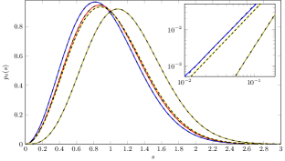
Figure S1: Comparison of theoretical and experimental distributions of local level spacings for the CUE spectra. Yellow curve displays $p(s)$ – the distribution of spacings between consecutive eigenlevels. Olive, blue and red curves represent the distribution of local spacings $p_{\ell}(s)$ for $\ell=0,1$ and 2 respectively. Experimental distributions are obtained from $2\times 10^{8}$ samples with $N=1024$ and $\varphi=\pi$. Dashed curves appearing on top of experimental curves display corresponding theoretical $N\rightarrow\infty$ laws given by Eqs. (S.55), (S.56a) and (S.57) for $p(s)$, Eq. (10a) for $p_{0}(s)$, Eq. (S.51) for $p_{1}(s)$ and Eq. (S.54) for $p_{2}(s)$. The inset shows magnified experimental distributions at the origin plotted on the log-log scale. The dashed lines indicate power law dependencies with the slope $2$ and $3$.

associated with the conditional two-point scalar kernel [3, 4]

$$K_{N-1}^{{\mathbb{T}}\,(\vartheta_{1},\dots,\vartheta_{\ell})}(x,y) = K_{N-1}^{{\mathbb{T}}}(x,y)$$ (S.35)

$$- \left[\begin{array}[]{c}K_{N-1}^{{\mathbb{T}}}(x,\vartheta_{1})\\ \vdots\\ K_{N-1}^{{\mathbb{T}}}(x,\vartheta_{\ell})\end{array}\right]^{T}\left[\begin{array}[]{ccc}K_{N-1}^{{\mathbb{T}}}(\vartheta_{1},\vartheta_{1})&\dots&K_{N-1}^{{\mathbb{T}}}(\vartheta_{1},\vartheta_{\ell})\\ \vdots&\ddots&\vdots\\ K_{N-1}^{{\mathbb{T}}}(\vartheta_{\ell},\vartheta_{1})&\dots&K_{N-1}^{{\mathbb{T}}}(\vartheta_{\ell},\vartheta_{\ell})\end{array}\right]^{-1}\left[\begin{array}[]{c}K_{N-1}^{{\mathbb{T}}}(\vartheta_{1},y)\\ \vdots\\ K_{N-1}^{{\mathbb{T}}}(\vartheta_{\ell},y)\end{array}\right].$$

Equations (S.19) and (S.22) supply the representation of $p_{\ell}(s;N)$ at $\beta=2$ in terms of the Fredholm determinant:

$$p_{\ell}(s;N) = \frac{1}{2\pi\Delta_{N}}\frac{1}{(\ell-1)!}\intop\ilimits@_{s}^{2\pi}d\varphi$$ (S.36)

$$\times \left(\prod_{j=1}^{\ell-1}\intop\ilimits@_{s}^{\varphi}\frac{d\vartheta_{j}}{2\pi}\right)\,{\rm det}_{1\leq i,j\leq\ell}\left[K_{N-1}^{\mathbb{T}}(\vartheta_{i},\vartheta_{j})\right]\big{|}_{\vartheta_{\ell}=s}{\rm det}\left(\openone-{\mathbb{K}}_{N-1}^{{\mathbb{T}}\;(s,\vartheta_{1},\dots,\vartheta_{\ell-1})}\big{|}_{(0,\varphi)}\right).$$

This result holds for $\ell=1,\dots,N-1$.

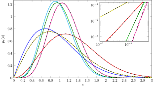
Figure S2: Distributions of local level spacings for the ${\rm COE}$ and ${\rm CSE}$ spectra. For the ${\rm COE}$ spectra: red and blue curves show experimental distributions of local spacings $p_{0}(s)$ and $p_{1}(s)$, respectively; yellow curve corresponds to the experimentally determined distribution of spacings between consecutive eigenlevels $p(s)$. For the ${\rm CSE}$ spectra: magenta and cyan curves show experimental distributions of local spacings $p_{0}(s)$ and $p_{1}(s)$, respectively; green curve displays the experimentally determined distribution of spacings between consecutive eigenlevels $p(s)$. The curves were produced by statistical analysis of $2\times 10^{7}$ samples with $N=1024$ and $\varphi=\pi$. The dashed lines on top of experimental curves show theoretical predictions for $p_{0}(s)$ and $p(s)$ determined by Eqs. (10a) and (S.55)–(S.57). The inset shows magnified experimental distributions at the origin plotted on the log-log scale. The dashed lines there indicate the predicted power law dependencies with the slopes $1$, $2$, $4$ and $5$ (from left to right).

(ii) Emergence of universal laws.—To deduce the universal laws for distributions of local spacings, one has to implement the scaling limit

$$p_{\ell}(s)=\lim_{N\rightarrow\infty}\frac{2\pi}{N}p_{\ell}\left(\frac{2\pi}{N}s;N\right)$$ (S.37)

in Eq. (S.36) provided $\ell$ is kept fixed. Since this scaling limit reduces the ${\rm TCUE}(N-1)$ scalar kernel [Eq. (S.23)] to the ${\rm Bessel}_{1}$ kernel [5]

$$K^{{\rm Bessel}_{1}}(x,y)=\lim_{N\rightarrow\infty}\frac{1}{N}K_{N-1}^{\mathbb{T}}\left(\frac{2\pi}{N}x,\frac{2\pi}{N}y\right)=\frac{\sin[\pi(x-y)]}{\pi(x-y)}-\frac{\sin[\pi x]}{\pi x}\frac{\sin[\pi y]}{\pi y}$$ (S.38)

defined by the formula [6, 7, 8]

$$K^{{\rm Bessel}_{a}}(x,y)=\frac{\pi}{2}\frac{\sqrt{xy}}{x-y}\Big{(}J_{a+1/2}(\pi x)J_{a-1/2}(\pi y)-J_{a+1/2}(\pi y)J_{a-1/2}(\pi x)\Big{)},$$ (S.39)

where $a>-1/2$ and $xy\geq 0$, the following Fredholm determinant representation emerges:

$$p_{\ell}(s) = \frac{1}{(\ell-1)!}\intop\ilimits@_{s}^{\infty}dt$$ (S.40)

$$\times \left(\prod_{j=1}^{\ell-1}\intop\ilimits@_{s}^{t}d\lambda_{j}\right)\,{\rm det}_{1\leq i,j\leq\ell}\left[K^{{\rm Bessel}_{1}}(\lambda_{i},\lambda_{j})\right]\big{|}_{\lambda_{\ell}=s}\,{\rm det}\left(\openone-{\mathbb{K}}^{{{\rm Bessel}_{1}}\;(s,\lambda_{1},\dots,\lambda_{\ell-1})}\big{|}_{(0,t)}\right).$$

Here,

$$\!\!\!\!\!\!\!\!\!\!\!\!\!\!\!\!K^{{\rm Bessel}_{1}\,(\lambda_{1},\dots,\lambda_{\ell})}(x,y) = K^{{\rm Bessel}_{1}}(x,y)$$ (S.50)

$$- \left[\begin{array}[]{c}K^{{\rm Bessel}_{1}}(x,\lambda_{1})\\ \vdots\\ K^{{\rm Bessel}_{1}}(x,\lambda_{\ell})\end{array}\right]^{T}\left[\begin{array}[]{ccc}K^{{\rm Bessel}_{1}}(\lambda_{1},\lambda_{1})&\dots&K^{{\rm Bessel}_{1}}(\lambda_{1},\lambda_{\ell})\\ \vdots&\ddots&\vdots\\ K^{{\rm Bessel}_{1}}(\lambda_{\ell},\lambda_{1})&\dots&K^{{\rm Bessel}_{1}}(\lambda_{\ell},\lambda_{\ell})\end{array}\right]^{-1}\left[\begin{array}[]{c}K^{{\rm Bessel}_{1}}(\lambda_{1},y)\\ \vdots\\ K^{{\rm Bessel}_{1}}(\lambda_{\ell},y)\end{array}\right]$$

is the conditional two-point ${\rm Bessel}_{1}$ kernel, see Eq. (S.35) for a similar structure.

For low values of $\ell$, the representation Eq. (S.40) is particularly useful for numerical evaluation of the local spacing distributions. For example, the distributions of the first ($\ell=1$) and the second ($\ell=2$) local spacings are given by the single

$$p_{1}(s)=K^{{\rm Bessel}_{1}}(s,s)\intop\ilimits@_{s}^{\infty}dt\,{\rm det}\left(\openone-{\mathbb{K}}^{{{\rm Bessel}_{1}}\;(s,t)}\big{|}_{(0,t)}\right)$$ (S.51)

and double

$$p_{2}(s) = \intop\ilimits@_{s}^{\infty}dt\,\intop\ilimits@_{s}^{t}d\lambda\,{\rm det}\left[\begin{array}[]{cc}K^{{\rm Bessel}_{1}}(s,s)&K^{{\rm Bessel}_{1}}(s,\lambda)\\ K^{{\rm Bessel}_{1}}(\lambda,s)&K^{{\rm Bessel}_{1}}(\lambda,\lambda)\end{array}\right]{\rm det}\left(\openone-{\mathbb{K}}^{{{\rm Bessel}_{1}}\;(s,\lambda)}\big{|}_{(0,t)}\right)$$ (S.54)

integrals, respectively. The Fredholm determinants therein can be evaluated numerically with the help of Bornemann’s MATLAB package [9].

Discussion of numerical tests.—In Fig. S1 we compare distributions of local spacing for numerically simulated large-dimensional ${\rm CUE}(N)$ spectra with theoretical predictions for $p_{0}(s)$, $p_{1}(s)$ and $p_{2}(s)$. The agreement is perfect. For $s\ll 1$, the distributions of zeroth $p_{0}(s)$ and first $p_{1}(s)$ local spacings show a cubic and quadratic slopes, in concert with the discussion above Eq. (11) of the main text. As $\ell$ grows, $p_{\ell}(s)$ quickly approaches $p(s)$; this is natural since the correlations between the spacings $s_{X}$ and $s_{X+\ell}$ containing $\ell$ eigenlevels apart [Eq. (21b)] weaken as $\ell$ grows.

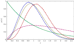
Figure S3: Comparison of theoretical and experimental distributions of local level spacings for zeros of the Riemann zeta function and spectra of irrational rectangular billiards. For the Riemann zeta function: red and blue curves represent the experimentally calculated local spacing distributions $p_{0}(s)$ and $p_{1}(s)$, respectively; yellow curve shows the experimentally determined distribution $p(s)$ between consecutive zeros. For rectangular billiards: magenta and cyan curves display experimentally determined local spacing distributions $p_{0}(s)$ and $p_{1}(s)$, respectively; green curve corresponds to the spacing distribution $p(s)$. Notice that for rectangular billiards $p(s)$ (green) and $p_{1}(s)$ (cyan) fluctuate around each other. Statistical analysis of both systems involved $10^{6}$ samples (see description of Test II in the main text for more details). The dashed lines show theoretical predictions for $p(s)$, $p_{0}(s)$ and $p_{1}(s)$. Theoretical curves for the Riemann zeta function coincide with those displayed in Fig. S1. Theoretical curves for the billiard spectra are given by Eq. (14) derived for the Poisson spectra.

In Fig. S2, we display the experimentally computed local distributions for large-dimensional ${\rm COE}(N)$ and ${\rm CSE}(N)$ spectra. For comparison with the theory and details of statistical analysis, the reader is referred to the caption.

In Fig. S3, our theoretical predictions are confronted with experimental distributions of local spacings determined for two real systems: the Riemann zeta function and irrational rectangular billiards.

The experimental curves obtained for nontrivial zeros of the Riemann zeta function follow closely the predictions derived for the ${\rm CUE}$ spectra. In distinction to the experimental ${\rm CUE}$ curves displayed in Fig. S1, the fluctuations in Fig. S3 are more pronounced. This is hardly surprising since $200$ times less samples were produced out of available data for nontrivial Riemann zeros.

The experimental curves for rectangular billiards are fundamentally different; they nicely follow the theoretical predictions [Eq. (14)] derived for the Poisson spectra. Even though there is no level repulsion in the Poisson spectra, the distribution of zeroth local spacing exhibits an effective linear repulsion between the eigenlevels located at the endpoints of the ‘inspected’ (zeroth) spacing. Remarkably, the distributions of all other local spacings ($\ell\neq 0$) coincide with $p(s)=\exp(-s)$. This phenomenon derives from the fact that consecutive level spacings in the Poisson spectra are completely uncorrelated.

Distribution of spacings between consecutive eigenlevels and the fifth Painlevé transcendent.—For comparison of experimental and theoretical results for the distribution $p_{0}^{(\beta)}(s)$ of zeroth local spacing [Eq. (10a)], we have used the following nonperturbative formulae for the distributions $p^{(\beta)}(s)$ of consecutive spacings ($\beta=1,2,4$):

$$p^{(\beta)}(s)=\frac{d^{2}}{ds^{2}}E^{(\beta)}(0;s),$$ (S.55)

where [10, 11]

$$E^{(2)}(0;s)=\exp\left(\intop\ilimits@_{0}^{2\pi s}\frac{\sigma_{0}(t)}{t}dt\right),$$ (S.56a)

$$E^{(1)}(0;s)=\exp\left(-\frac{1}{2}\intop\ilimits@_{0}^{2\pi s}\sqrt{-\frac{d}{dt}\frac{\sigma_{0}(t)}{t}}dt\right)\,\sqrt{E^{(2)}(0;s)}$$ (S.56b)

and

$$E^{(4)}(0;s/2)=\cosh\left(\frac{1}{2}\intop\ilimits@_{0}^{2\pi s}\sqrt{-\frac{d}{dt}\frac{\sigma_{0}(t)}{t}}dt\right)\,\sqrt{E^{(2)}(0;s)}$$ (S.56c)

are the gap formation probabilities $E^{(\beta)}(0;s)$ for the ${\rm Sine}_{\beta}$ point process. Here, $\sigma_{0}(t)$ is a fifth Painléve transcendent satisfying the nonlinear differential equation

$$(t\sigma_{0}^{\prime\prime})^{2}+(t\sigma_{0}^{\prime}-\sigma_{0})\left(t\sigma_{0}^{\prime}-\sigma_{0}+4(\sigma_{0}^{\prime})^{2}\right)=0$$ (S.57a)

subject to the boundary condition

$$\sigma_{0}(t)=-\frac{t}{2\pi}-\left(\frac{t}{2\pi}\right)^{2}+{\mathcal{O}}(t^{3})$$ (S.57b)

as $t\rightarrow 0$. Notice that, contrary to the phenomenological Wigner-surmise formulae, the above representations are exact.

A fifth Painlevé transcendent $\sigma_{0}(t)$ [Eq. (S.57)] as well as the integrals appearing in Eqs. (S.56a)–(S.56c) were determined numerically by employing a standard MATLAB ordinary differential equations (ODE) solver applied to the Chazy form of Eq. (S.57a), see Eq. (B.7) of Ref. [12]. To produce initial conditions for the ODE solver away from the singularity at $t=0$, we used a Taylor polynomial of a high degree generated analytically through the recurrence relation Eq. (B.8) of Ref. [12] after setting $\zeta=1$ therein.

IV 3. On improving statistics for ratios $\varrho_{\ell}^{\rm loc}$ of means of local spacings

The statistical analysis of the ratios $\varrho_{\ell}^{\rm loc}$ in Test III was based on $10^{6}$ samples of raw spectra with a single reference point $\varphi=0$. Let us stress that statistics of comparable quality for $\varrho_{\ell}^{\rm loc}$ could be obtained with a significantly smaller number ($M$) of samples. Indeed, choosing either deterministically or at random a sufficiently large set of pre-defined local reference points $\{\varphi_{1},\varphi_{2},\dots,\varphi_{Q}\}$, one could first evaluate sample averages $\{\langle s_{\ell}^{\rm loc}(\varphi_{\alpha})\rangle_{M}\}|_{\alpha=1}^{Q}$ of local spacings separately for each $\varphi_{\alpha}$ and then use them to calculate a set of local ratios

$$\rho^{\textrm{loc}}_{\ell}(\varphi_{\alpha})=\frac{\langle s_{\ell}^{\textrm{loc}}(\varphi_{\alpha})\rangle_{M}}{\langle s_{0}^{\textrm{loc}}(\varphi_{\alpha})\rangle_{M}}$$ (S.58)

for each $\ell$ and $\alpha=1,2,\dots,Q$. Since the theoretical expectation values of these ratios should not depend on a particular value of $\varphi_{\alpha}$, one may further average them over $\alpha$

$$\varrho^{\rm loc}_{\ell}=\frac{1}{Q}\sum_{\alpha=1}^{Q}\rho^{\rm loc}_{\ell}(\varphi_{\alpha})$$ (S.59)

to improve the statistics. The same strategy can be used to improve statistics of local spacings in the unfolded spectra, see Test I.

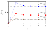
Figure S4: The mean values $\langle r_{\ell}^{\rm loc}\rangle$ of the local $r$-ratios calculated for large-dimensional ${\rm COE}(N)$ (blue dots), ${\rm CUE}(N)$ (red squares) and ${\rm CSE}(N)$ (brown diamonds) matrix models. For simulation parameters, see caption to Table 1. The values $\langle r^{(\beta)}\rangle$, represented by dashed lines, are approximately equal [14] to $1.7781$ for $\beta=1$, $1.3684$ for $\beta=2$, and $1.1769$ for $\beta=4$.

V 4. On a local version of Oganesyan-Huse-Bogomolny $r$-ratio

A notion of local level spacings introduced in the Letter raises a natural question about a possible relation between the Oganesyan-Huse-Bogomolny $r$-ratio [13, 14] and its local version

$$r_{\ell}^{{\rm loc}}=\frac{s_{\ell+1}^{{\rm loc}}}{s_{\ell}^{{\rm loc}}},$$ (S.60)

where $s_{\ell}^{{\rm loc}}$ is the (fluctuating) $\ell$-th local spacing with respect to the reference point $\varphi$. Similarly to the $r$-statistics, this ratio is also barely affected by a system dependent mean level density. Yet, contrary to the $r$-ratio, the average $\langle r_{\ell}^{\rm loc}\rangle$ is not a constant anymore, being $\ell$-dependent. More precisely, it is described by universal sequences $\{\langle r_{\ell}^{\rm loc}\rangle\}$ which depend on the spectral universality class and system symmetry; the first member of these sequences is always unity [15]

$$\langle r_{0}^{\rm loc}\rangle=1.$$ (S.61)

A truly nonperturbative calculation of $\langle r_{\ell}^{\rm loc}\rangle$ for $\ell\neq 0$ is a nontrivial problem.

In Fig. S4 we show the results of numerical simulations of local $r$-ratios, performed for large-dimensional ${\rm C}\beta{\rm E}(N)$ matrix models. The graphs suggest that, as $\ell$ grows, the universal sequences $\langle r_{\ell}^{\rm loc}\rangle$ start to approach the universal values $\langle r^{(\beta)}\rangle$ due to Bogomolny and co-authors [14]. This is unsurprising since the effects of locality fade away as $\ell$ increases.

In the Poisson spectra, characterized by completely uncorrelated consecutive spacings, the memory of locality is lost immediately. Indeed, explicit calculation of the distribution functions $p_{\ell}(r)$ of local $r$-ratios yields

$$p_{\ell}(r)={\mathbb{E}}_{{\bm{\theta}}}\left[\delta\left(r-r_{\ell}^{\rm loc}\right)\right]=\left\{\begin{array}[]{cc}\displaystyle\frac{2}{(1+r)^{3}},&\ell=0;\\ \displaystyle\frac{1}{(1+r)^{2}},&\ell\geq 1.\end{array}\right.$$ (S.64)

Hence, starting with $\ell=1$, the fluctuations of local ratios become indistinguishable from the Oganesyan-Huse-Bogomolny $r$-ratio whose distribution equals [14]

$$p(r)=\frac{1}{(1+r)^{2}}.$$ (S.65)

References

[1] T. Guhr, A. Müller-Groeling, and H. A. Weidenmüller:
Random-matrix theories in quantum physics: Common concepts.
Phys. Reports 299, 189 (1998).
[2] H.-J. Stöckmann:
Quantum Chaos: An Introduction (Cambridge University Press, Cambridge, 1999).
[3] F. Haake:
Quantum Signatures of Chaos (Springer, Berlin, 2001).
[4] O. Bohigas, M. J. Giannoni, and C. Schmit:
Characterization of chaotic quantum spectra and universality of level fluctuation laws.
Phys. Rev. Lett. 52, 1 (1984).
[5] S. W. McDonald and A. N. Kaufman:
Spectrum and eigenfunctions for a Hamiltonian with stochastic trajectories.
Phys. Rev. Lett. 42, 1189 (1979).
[6]
G. Casati, F. Valz-Gris, and I. Guarnieri:
On the connection between quantization of nonintegrable systems and statistical theory of spectra.
Lett. Nuovo Cimento 28, 279 (1980).
[7] M. V. Berry:
Quantizing a classically ergodic system: Sinai’s billiard and the KKR method.
Ann. Phys. 131, 163 (1981).
[8] G. M. Zaslavsky:
Stochasticity in quantum systems.
Phys. Rep. 80, 157 (1981).
[9] M. L. Mehta, Random Matrices (Amsterdam: Elsevier, 2004).
[10] P. J. Forrester, Log-Gases and Random Matrices (Princeton: Princeton University Press, 2010).
[11] M. V. Berry and M. Tabor:
Level clustering in the regular spectrum.
Proc. R. Soc. A 356, 375 (1977).
[12] The number variance measures fluctuations of the number of eigenlevels in the interval of given length.
[13] M. Jimbo, T. Miwa, Y. Môri, and M. Sato:
Density matrix of an impenetrable Bose gas and the fifth Painlevé transcendent.
Physica D 1, 80 (1980).
[14] C. A. Tracy and H. Widom: Introduction to random matrices, in: Geometric and Quantum Aspects of Integrable Systems,
edited by G. F. Helminck. Lecture Notes in Physics 424, 103 (Berlin: Springer-Verlag, 1993).
[15] P. J. Forrester and A. M. Odlyzko:
Gaussian unitary ensemble eigenvalues and Riemann zeta function zeros: A nonlinear equation for a new statistic.
Phys. Rev. E 54, R4493 (1996).
[16] A. Relaño, J. M. G. Gómez, R. A. Molina, J. Retamosa, and E. Faleiro:
Quantum chaos and noise.
Phys. Rev. Lett. 89, 244102 (2002).
[17] R. Riser, V. Al. Osipov, and E. Kanzieper:
Power spectrum of long eigenlevel sequences in quantum chaotic systems.
Phys. Rev. Lett. 118, 204101 (2017).
[18] R. Riser, V. Al. Osipov, and E. Kanzieper:
Nonperturbative theory of power spectrum in complex systems.
Ann. Phys. 413, 168065 (2020).
[19] R. Riser and E. Kanzieper:
Power spectrum of the circular unitary ensemble.
Physica D 444, 133599 (2023).
[20] A. M. Odlyzko:
On the distribution of spacings between zeros of the zeta function.
Math. Comput. 48, 273 (1987).
[21] R. Riser, P. Tian, and E. Kanzieper:
Power spectra and auto-covariances of level spacings beyond the Dyson conjecture.
Phys. Rev. E. 107, L032201 (2023).
[22] V. Oganesyan and D. A. Huse:
Localization of interacting fermions at high temperature.
Phys. Rev. B 75, 155111 (2007).
[23] Y. Y. Atas, E. Bogomolny, O. Giraud, and G. Roux:
Distribution of the ratio of consecutive level spacings in random matrix ensembles.
Phys. Rev. Lett. 110, 084101 (2013).
[24]
A. M. García-García, and J. J. M. Verbaarschot:
Spectral and thermodynamic properties of the Sachdev-Ye-Kitaev model.
Phys. Rev. D 94, 126010 (2016).
[25] M. Akila, D. Waltner, B. Gutkin, P. Braun, and T. Guhr:
Semiclassical identification of periodic orbits in a quantum many-body system.
Phys. Rev. Lett. 118, 164101 (2017).
[26] B. Bertini, P. Kos, and T. Prosen:
Exact spectral form factor in a minimal model of many-body quantum chaos.
Phys. Rev. Lett. 121, 264101 (2018).
[27] Y. Liao, A. Vikram, and V. Galitski:
Many-body level statistics of single-particle quantum chaos.
Phys. Rev. Lett. 125, 250601 (2020).
[28] T. A. Sedrakyan and K. B. Efetov:
Supersymmetry method for interacting chaotic and disordered systems:
The Sachdev-Ye-Kitaev model.
Phys. Rev. B 102, 075146 (2020).
[29] F. Monteiro, T. Micklitz, M. Tezuka, and A. Altland:
Minimal model of many-body localization.
Phys. Rev. Res. 3, 013023 (2021).
[30] K. Richter, J. D. Urbina, and S. Tomsovic:
Semiclassical roots of universality in many-body quantum chaos.
J. Phys. A: Math. Theor. 55, 453001 (2022).
[31] S. Shivam, A. De Luca, D. A. Huse, and A. Chan:
Many-body quantum chaos and emergence of Ginibre ensemble.
Phys. Rev. Lett. 130, 140403 (2023).
[32] A. Andreanov, M. Carrega, J. Murugan, J. Olle, D. Rosa, and R. Shir:
From Dyson models to many-body quantum chaos.
arXiv:2302.00917 (2023).
[33] Since the mean of such a ratio diverges for the Poisson spectra, one actually deals with a minimum between a ratio of spacings and its inverse.
[34] In the context of dissipative quantum chaotic systems, characterized by complex-valued spectra, a definition the -statistics should properly be modified, see recent study [35].
[35] L. Sá, P. Ribeiro, and T. Prosen:
Complex spacing ratio: A signature of dissipative quantum chaos.
Phys. Rev. X 10, 021019 (2020).
[36] Other statistical indicators probing correlations between consecutive level spacings
include: (i) the distribution of spacings between nearest-neighbor eigenlevels [15] (not to be confused
with distribution of spacings between consecutive eigenlevels), (ii) auto-covariances of level spacings [9, 37, 21], and (iii) their power spectrum [20, 21].
[37]
O. Bohigas, P. Lebœuf, and M. J. Sánchez:
Spectral spacing correlations for chaotic and disordered systems.
Foundations of Physics 31, 489 (2001).
[38] N. Masuda and T. Hiraoka:
Waiting time paradox in 1922.
Northeast J. Complex Systems 2, 1 (2020).
[39] W. Feller, An Introduction to Probability Theory and Its Applications, Vol. II (New York: John Wiley and Sons, 1971).
[40] A. Pal, S. Kostinski, and S. Reuveni:
The inspection paradox in stochastic resetting.
J. Phys. A: Math. Theor. 55, 021001 (2022).
[41] K. Maples, J. Najnudel, and A. Nikeghbali:
Strong convergence of eigenangles and eigenvectors for the circular unitary ensemble.
Ann. Probab. 47, 2417 (2019).
[42] R. Killip and M. Stoiciu:
Eigenvalue statistics for CMV matrices: From Poisson to clock via random matrix ensembles.
Duke Math. J. 146 361 (2009).
[43] B. Valkó and B. Virág:
The operator.
Invent. Math. 209, 275 (2017).
[44] For appearance of the point process in nonperturbative calculations of the power
spectrum in quantum chaotic systems see Ref. [19, 21].
[45] P. J. Forrester and N. S. Witte:
Exact Wigner surmise type evaluation of the spacing distribution in the bulk of the scaled random matrix ensembles.
Lett. Math. Phys. 53, 195 (2000).
[46] P. J. Forrester:
Spacing distributions in random matrix ensembles, in:
Recent Perspectives in Random Matrix Theory and Number Theory, edited by
F. Mezzadri and N. C. Snaith. London Math. Soc. Lecture Note Series 322, p. 279
(Cambridge University, Cambridge, England, 2005).
[47] P. Tian, R. Riser, and E. Kanzieper: Supplemental Material to this Letter (2023).
[48] The local spacings and have the same distributions due to the -periodicity and the mirror symmetry.
[49] Notice that the answer does not depend on .
[50] In the mathematical literature, such a conditioned point process corresponds to the Palm measure of the process, see Ref. [51]. In fact, ensemble mentioned below Eq. (9d) represents the Palm process for the Dyson triad .
[51] S. Ghosh:
Palm measures and rigidity phenomena in point processes.
Electron. Commun. Probab. 21, 1 (2016).
[52] F. Bornemann:
On the numerical evaluation of distributions in random matrix theory: A review.
Markov Processes Relat. Fields 16, 803 (2010).
[53] A. M. Odlyzko, private communication.
[54] G. A. Hiary and A. M. Odlyzko:
Numerical study of the derivative of the Riemann zeta function at zeros.
Commentarii Mathematici Universitatis Sancti Pauli 60, 47 (2011).
[55] A. M. Odlyzko:
The -nd zero of the Riemann zeta function, in:
Dynamical, Spectral, and Arithmetic Zeta Functions, edited by
M. L. Lapidus and M. van Frankenhuysen.
Contemp. Math. Series, vol. 290, p. 139
(Amer. Math. Soc, Providence, RI, 2001).
[56] R. Riser and E. Kanzieper:
Power spectrum and form factor in random diagonal matrices and integrable billiards.
Ann. Phys. 425, 168393 (2021).
[57] We remark that experimental values of computed for the Riemann zeros lied slightly outside of the confidence interval. As the discrepancy became more pronounced for lower lying zeros (around -th zero) of the Riemann zeta function, we attribute a mismatch to the nonuniversal finite energy effects.
[58] S. Sachdev and J. Ye:
Gapless spin fluid ground state in a random quantum Heisenberg magnet.
Phys. Rev. Lett. 70 3339 (1993).
[59] A. Kitaev:
A simple model of quantum holography.
KITP Program: Entanglement in Strongly-Correlated Quantum Matter.
(Lectures delivered on April 7 and May 27, 2015).
[60] For historical introduction and relation to the earlier work, see Ref. [24].
[61] A. M. García-García, and J. J. M. Verbaarschot:
Analytical spectral density of the Sachdev-Ye-Kitaev model at finite .
Phys. Rev. D 96, 066012 (2017);
J. S. Cotler, G. Gur-Ari, M. Hanada, J. Polchinski, P. Saad, S. H. Shenker, D. Stanford, A. Streicher, and M. Tezuka:
Black holes and random matrices.
J. High Energy Phys. 2017, 118 (2017).
[62] Y.-Z. You, A. W. W. Ludwig, and C. Xu:
Sachdev-Ye-Kitaev model and thermalization on the boundary of many-body localized fermionic symmetry-protected topological states.
Phys. Rev. B 95, 115150 (2017).
[63] Y. Ameur, F. Marceca, and J. L. Romero:
Gaussian beta ensembles: the perfect freezing transition and its characterization in terms of Beurling-Landau densities.
arXiv:2205.15054 (2022).

References

[1] R. Riser, V. Al. Osipov, and E. Kanzieper:
Nonperturbative theory of power spectrum in complex systems.
Ann. Phys. 413, 168065 (2020).
[2] A. Borodin and A. Soshnikov:
Janossy densities. I. Determinantal ensembles.
J. Stat. Phys. 113, 595 (2003);
A. Soshnikov:
Janossy densities II. Pfaffian ensembles.
J. Stat. Phys. 113, 611 (2003).
[3] S. M. Nishigaki:
Tracy–Widom method for Jánossy density and joint distribution of extremal eigenvalues of random matrices.
Prog. Theor. Exp. Phys. 2021, 113A01 (2021).
[4] A. Edelman and S. Jeong:
The conditional DPP approach to random matrix distributions.
arXiv:2304.09319 (2023).
[5] Notice that the very same kernel has previously surfaced in the studies of the distribution of spacings between nearest-neighbor eigenlevels, which is yet another statistics probing the correlations between traditional level spacings. See Ref. [15] in the Letter.
[6] T. Nagao and K. Slevin:
Nonuniversal correlations for random matrix ensembles.
J. Math. Phys. 34, 2075 (1983).
[7] G. Akemann, P. H. Damgaard, U. Magnea, and S. Nishigaki:
Universality of random matrices in the microscopic limit and the Dirac operator spectrum.
Nucl. Phys. B 487, 721 (1997).
[8] E. Kanzieper and V. Freilikher:
Random-matrix models with the logarithmic-singular level confinement:
Method of fictitious fermions.
Phil. Magazine B 77, 1161 (1998).
[9] F. Bornemann:
On the numerical evaluation of distributions in random matrix theory: A review.
Markov Processes Relat. Fields 16, 803 (2010).
[10] P. J. Forrester and N. S. Witte:
Exact Wigner surmise type evaluation of the spacing distribution in the bulk of the scaled random matrix ensembles.
Lett. Math. Phys. 53, 195 (2000).
[11] P. J. Forrester:
Spacing distributions in random matrix ensembles, in:
Recent Perspectives in Random Matrix Theory and Number Theory, edited by
F. Mezzadri and N. C. Snaith. London Math. Soc. Lecture Note Series 322, p. 279
(Cambridge University, Cambridge, England, 2005).
[12] R. Riser and E. Kanzieper:
Power spectrum of the circular unitary ensemble.
Physica D 444, 133599 (2023).
[13] V. Oganesyan and D. A. Huse:
Localization of interacting fermions at high temperature.
Phys. Rev. B 75, 155111 (2007).
[14] Y. Y. Atas, E. Bogomolny, O. Giraud, and G. Roux:
Distribution of the ratio of consecutive level spacings in random matrix ensembles.
Phys. Rev. Lett. 110, 084101 (2013).