Exotic eigenvalues and analytic resolvent for a graph with a shrinking edge

Abstract.

We consider a metric graph consisting of two edges, one of which has length $\varepsilon$ which we send to zero. On this graph we study the resolvent and spectrum of the Laplacian subject to a general vertex condition at the connecting vertex. Despite the singular nature of the perturbation (by a short edge), we find that the resolvent depends analytically on the parameter $\varepsilon$. In contrast, the negative eigenvalues escape to minus infinity at rates that could be fractional, namely, $\varepsilon^{0}$, $\varepsilon^{-2/3}$ or $\varepsilon^{-1}$. These rates take place when the corresponding eigenfunction localizes, respectively, only on the long edge, on both edges, or only on the short edge.

1. Introduction

Differential operators on metric graphs arise in numerous applied problems, for example, as effective descriptions of physical processes taking place on thin branching domains [20, 15, 14, 23]. Spectral properties of such operators depend on many factors, such as the differential expression itself, vertex matching conditions, connectivity (topology) of the graph, as well as edge lengths. In this study we focus on a graph which consists of edges of two length scales, of order one and of order $\varepsilon\to 0$. Such problems arise naturally in the studies of metamaterials, where a large-scale structure may contain small-scale inclusions which substantially alters the overall physical properties [11, 12, 21].

While analytic dependence of a compact graph’s spectrum on the edge lengths was known for some time [4], this result specifically excluded the case of edges shrinking to a point. Substantial progress was achieved in four recent publications [6, 10, 9, 8], where general positive results were established under varying “non-resonance” conditions, which, informally speaking, prevent eigenfunctions from localizing on the shrinking part of the graph. In this work we thoroughly study a simple example that violates these conditions.

Despite the simplicity of the example, we catalogue a variety of curious behaviors. To give a preview, consider the operator acting as $-\frac{d^{2}}{dx^{2}}$ on the space $L^{2}((-\varepsilon,0))\oplus L^{2}((0,1))$, supplied with the following vertex conditions

$$u^{\prime}(-\varepsilon)=0,\qquad u^{\prime}(0-)=u(0+),\qquad u^{\prime}(0+)=-u(0-),\qquad u(1)=0.$$ (1.1)

An a priori bound by Kuchment [19] (see also [18, 7]) estimates the bottom of the spectrum to be $\gtrsim-1/{s}_{\min}$, where ${s}_{\min}$ is the shortest edge length, i.e. $\varepsilon$. Surprisingly, in this particular example, the lowest eigenvalue tends to $-\infty$ at a fractional rate, namely $\lambda_{1}=-\varepsilon^{-2/3}+O(\varepsilon^{2/3})$.

It is interesting to compare this example to the problem of absorption of eigenvalues into the continuous spectrum, studied by Simon in [24]. Rescaling all edge lengths by $\varepsilon$ and extending the long edge to infinity, we arrive at the eigenvalue problem for the Laplacian on $(-1,0)\cup(0,\infty)$ with vertex conditions

$$u^{\prime}(-1)=0,\qquad u^{\prime}(0-)=\varepsilon u(0+),\qquad u^{\prime}(0+)=-\varepsilon u(0-).$$ (1.2)

Here, the lone negative eigenvalue approaches the continuous spectrum at $[0,\infty)$ at the rate $\varepsilon^{4/3}$. In [24, end of Sec. 2], Simon argued that one can obtain any rate $\varepsilon^{\alpha}$, $\alpha\geqslant 1$, by considering a fractional power of Laplacian. Here we obtain a fractional rate for the Laplacian itself and only with linear dependence of the vertex conditions on the parameter $\varepsilon$.

In this work we take this two-edge graph and search through all possible vertex conditions at the connecting vertex, in order to classify all possible rates attainable by the negative eigenvalues and, through a detailed study of the resolvent and the eigenfunctions, understand the circumstances in which the fractional rates arise. Interestingly, we find that the leading order rates can be $\varepsilon^{0}$, $\varepsilon^{-2/3}$ or $\varepsilon^{-1}$ and nothing else. This encourages us to conjecture that the same holds for arbitrary graphs with edge lengths of two scales.

2. Problem setting and the main results

We consider the graph $\Gamma_{\varepsilon}$ consisting of an edge ${s}_{\varepsilon}$ of length $\varepsilon$ connected to an edge $e$ of length $1$, see Figure 1; here $\varepsilon$ is a small positive parameter. The internal vertex connecting the two edges is denoted by $v_{c}$, while the other two vertices being the end-points of the edges ${s}_{\varepsilon}$ and $e$ are respectively denoted by $v_{\varepsilon}$ and $v$. On the edges we introduce variables, which are respectively denoted by $x_{\varepsilon}$ and $x$. The orientation is fixed by letting $x_{\varepsilon}$ range from 0 at $v_{\varepsilon}$ to $\varepsilon$ at $v_{c}$ and $x$ range from 0 at $v_{1}$ to $1$ at $v_{c}$.

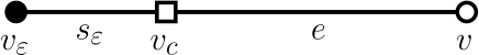
Figure 1. The graph $\Gamma_{\varepsilon}$. The vertex conditions are Neumann at $v_{\varepsilon}$, Dirichlet at $v$, and arbitrary at $v_{c}$.

We consider the self-adjoint operator $\mathcal{H}_{\varepsilon}$ on $L_{2}(\Gamma_{\varepsilon}):=L_{2}({s}_{\varepsilon})\oplus L_{2}(e)$, acting as

$$\mathcal{H}_{\varepsilon}\colon(u_{\varepsilon},u)\mapsto\left(-\frac{d^{2}u_{\varepsilon}}{dx_{\varepsilon}^{2}},-\frac{d^{2}u}{dx^{2}}\right)$$ (2.1)

with the domain $\operatorname{\mathfrak{D}}(\mathcal{H}_{\varepsilon})$ consisting of the functions $(u_{\varepsilon},u)\in H^{2}({s}_{\varepsilon})\oplus H^{2}(e)$ satisfying the boundary conditions

$$u_{\varepsilon}^{\prime}(0)=0,\qquad u(0)=0,\qquad\mathrm{P}\mathrm{U}=0,\qquad\mathrm{Q}\mathrm{U}^{\prime}=\mathrm{T}\mathrm{Q}\mathrm{U},$$ (2.2)

where

$$\mathrm{U}:=\begin{pmatrix}u_{\varepsilon}(\varepsilon)\\ u(1)\end{pmatrix},\qquad\mathrm{U}^{\prime}:=\begin{pmatrix}-u_{\varepsilon}^{\prime}(\varepsilon)\\ -u^{\prime}(1)\end{pmatrix},$$ (2.3)

$\mathrm{P}$ is an arbitrary orthogonal projection operator acting in $\mathbb{C}^{2}$, and $\mathrm{T}$ is an arbitrary self-adjoint operator acting on the range of $Q:=\mathrm{I}-\mathrm{P}$. By Theorem 1.4.4 of [5], the last two conditions in (2.2) represent arbitrary self-adjoint conditions at the vertex $v_{c}$ and the introduced operator is self-adjoint.

Since the operator $\mathcal{H}_{\varepsilon}$ is defined on a compact graph, its resolvent is a compact operator in $L_{2}(\Gamma_{\varepsilon})$ and its spectrum consists of discrete eigenvalues, which can accumulate at infinity only. The main aim of this work is to study the behavior of the resolvent and eigenvalues of the operator $\mathcal{H}_{\varepsilon}$ as $\varepsilon$ goes to zero. Specifically, we focus on the negative eigenvalues — and the corresponding eigenfunctions — as their behavior is most strongly affected by the “singular” limit $\varepsilon\to 0$.

We further parametrize vertex conditions (2.2) by considering the following three cases.

1. If $\operatorname{rank}\mathrm{P}=2$, then

   $$\mathrm{P}=\mathrm{I},\qquad\mathrm{Q}=0,\qquad\mathrm{T}=0.$$ (2.4)

   This case corresponds to the (decoupled) Dirichlet conditions at the central vertex.

2. If $\operatorname{rank}\mathrm{P}=1$, then the matrices $\mathrm{P}$ and $\mathrm{Q}$ can be represented as

   $$\mathrm{P}=\begin{pmatrix}\frac{1}{\sqrt{1+|z|^{2}}}\\ \frac{\overline{z}}{\sqrt{1+|z|^{2}}}\end{pmatrix}\begin{pmatrix}\frac{1}{\sqrt{1+|z|^{2}}}&\frac{z}{\sqrt{1+|z|^{2}}}\end{pmatrix}=\begin{pmatrix}\frac{1}{1+|z|^{2}}&\frac{z}{1+|z|^{2}}\\ \frac{\bar{z}}{1+|z|^{2}}&\frac{|z|^{2}}{1+|z|^{2}}\end{pmatrix},\qquad z\in\mathbb{C}\cup\{\infty\},$$ (2.5)

   $$\mathrm{Q}=\begin{pmatrix}\frac{|z|^{2}}{1+|z|^{2}}&-\frac{z}{1+|z|^{2}}\\ -\frac{\bar{z}}{1+|z|^{2}}&\frac{1}{1+|z|^{2}}\end{pmatrix},$$

   and $T$ acts as a multiplication by $\mu\in\mathbb{R}$. This case includes Neumann-Kirchhoff ($z=-1$, $\mu=0$) and delta-type conditions ($z=-1$, $\mu\neq 0$). When $z=0$ or $z=\infty$, the central vertex decouples into one Dirichlet and one Neumann condition.

3. If $\operatorname{rank}\mathrm{P}=0$, then

   $$\mathrm{P}=0,\qquad\mathrm{Q}=\mathrm{I},\qquad\mathrm{T}=\begin{pmatrix}a&c\\ \bar{c}&b\end{pmatrix}$$ (2.6)

   with some $a,b\in\mathbb{R}$, $c\in\mathbb{C}$. This case corresponds to a generalized Robin condition $\mathrm{U}^{\prime}=\mathrm{T}\mathrm{U}$, which is decoupled if $\mathrm{T}$ is diagonal.

Our main results are as follows.

Theorem 1.

The operator $\mathcal{H}_{\varepsilon}$ can have at most two negative eigenvalues. Each eigenvalue is simple and comes in one of the three possible types (in the description below, $\Lambda_{0}$ is a function holomorphic at 0 and satisfying $\Lambda_{0}(0)\neq 0$, $\Lambda_{1}$ is a smooth function satisfying the estimate $\Lambda_{1}(s)=O\big{(}e^{-\frac{C}{s}}\big{)}$ for small positive $s$ and a positive constant $C$, and $\alpha>0$ is a real constant):

1. a bounded eigenvalue,

   $$\lambda(\varepsilon)=-\Lambda_{0}^{2}(\varepsilon)=-\alpha+O(\varepsilon),$$ (2.7)

2. an eigenvalue depending on the square root $\varepsilon^{\frac{1}{2}}$,

   $$\lambda(\varepsilon)=-\varepsilon^{-1}\left(\Lambda_{0}(\varepsilon^{\frac{1}{2}})+\Lambda_{1}(\varepsilon^{\frac{1}{2}})\right)^{2}=-\alpha\varepsilon^{-1}+O(\varepsilon^{-\frac{1}{2}}),$$ (2.8)

3. an eigenvalue depending on the cubic root $\varepsilon^{\frac{1}{3}}$,

   $$\lambda(\varepsilon)=-\varepsilon^{-\frac{2}{3}}\left(\Lambda_{0}(\varepsilon^{\frac{1}{3}})+\Lambda_{1}(\varepsilon^{\frac{1}{3}})\right)^{2}=-\alpha\varepsilon^{-\frac{2}{3}}+O(\varepsilon^{-\frac{1}{3}}).$$ (2.9)

The negative eigenvalues exist only in the cases specified in Table 1, where $\kappa_{1}$ is the root of

$$\kappa\coth\kappa=-\mu(1+|z|^{2}),$$ (2.10)

and $\kappa_{0}$ is the root of

$$\kappa\coth\kappa=\frac{|c|^{2}-ab}{a},\quad a\neq 0,\qquad\text{or}\qquad\kappa\coth\kappa=-b,\quad a=0,\quad c=0.$$ (2.11)

Conditions			type(B)	type(S)	type(C)
$\operatorname{rank}P=1$	$z=\infty$	$\mu<0$		✓$\alpha=|\mu|$
	$z\neq\infty$	$\mu(1+|z|^{2})<-1$	✓$\alpha=\kappa_{1}^{2}$
$\operatorname{rank}P=0$	$a<0$	$|c|^{2}<a(b+1)$	✓$\alpha=\kappa_{0}^{2}$	✓$\alpha=|a|$
		$|c|^{2}\geqslant a(b+1)$		✓$\alpha=|a|$
	$a=0$	$c=0$, $b+1<0$	✓$\alpha=\kappa_{0}^{2}$
		$c\neq 0$			✓$\alpha=|c|^{4/3}$
	$a>0$	$|c|^{2}>a(b+1)$	✓$\alpha=\kappa_{0}^{2}$

Table 1. Description of the vertex condition which lead to negative eigenvalues. The coefficient $\alpha$ of the leading term in (2.7)-(2.9) is specified in the corresponding column. When no coefficient $\alpha$ is specified, there is no eigenvalue of the corresponding type. If the vertex conditions do not fit into either of the listed cases, there are no negative eigenvalues. For explanations and examples of the vertex conditions, see (2.4)-(2.6).

Theorem 2.

As $\varepsilon\to 0+$, the normalized eigenfunctions of the operator $\mathcal{H}_{\varepsilon}$ associated with its negative eigenvalues satisfy

$$\big{\|}\psi|_{s_{\varepsilon}}\big{\|}^{2}=O(\varepsilon), \big{\|}\psi|_{e}\big{\|}^{2}=1+O(\varepsilon) \text{for eigenvalue of type (B)},$$ (2.12)

$$\big{\|}\psi|_{s_{\varepsilon}}\big{\|}^{2}=1+O(\varepsilon^{1/2}), \big{\|}\psi|_{e}\big{\|}^{2}=O(\varepsilon^{1/2}) \text{for eigenvalue of type (S)},$$ (2.13)

$$\big{\|}\psi|_{s_{\varepsilon}}\big{\|}^{2}=\frac{2}{3}+O(\varepsilon^{1/3}), \big{\|}\psi|_{e}\big{\|}^{2}=\frac{1}{3}+O(\varepsilon^{1/3}) \text{for eigenvalue of type (C)}.$$ (2.14)

It is interesting to note that in cases (S) and (C) a non-vanishing proportion of the eigenfunction’s norm localizes on the edge of vanishing length.

To fully describe the resolvent we need to introduce further notation. We let ${s}:=(0,1)$ and introduce the bounded operator $\mathcal{S}_{\varepsilon}:L_{2}({s})\to L_{2}({s}_{\varepsilon})$ acting as $(\mathcal{S}_{\varepsilon}u)(x):=u(\frac{x}{\varepsilon})$. The mapping $\mathcal{S}_{\varepsilon}\oplus\mathcal{I}$ is an isomorphism between linear spaces $L_{2}({s})\oplus L_{2}(e)$ and $L_{2}(\Gamma_{\varepsilon})=L_{2}({s}_{\varepsilon})\oplus L_{2}(e)$; we stress that this isomorphism does not preserve the $L_{2}$-norm. By $\mathcal{P}_{s}:L_{2}(\Gamma_{\varepsilon})\to L_{2}({s}_{\varepsilon})$ and $\mathcal{P}_{e}:L_{2}(\Gamma_{\varepsilon})\to L_{2}(e)$ we denote the natural restriction operators

$$\mathcal{P}_{s}:(u_{\varepsilon},u)\mapsto u_{\varepsilon},\qquad\mathcal{P}_{e}:(u_{\varepsilon},u)\mapsto u.$$ (2.15)

Since the operator $\mathcal{H}_{\varepsilon}$ is self-adjoint, its resolvent $(\mathcal{H}_{\varepsilon}-\lambda)^{-1}$ is well-defined for $\lambda\in\mathbb{C}\setminus\mathbb{R}$. We introduce two auxiliary operators on the space $L_{2}({s})\oplus L_{2}(e)$ by the formulas

$$\mathcal{R}_{e}(\varepsilon,\lambda):=\mathcal{P}_{e}(\mathcal{H}_{\varepsilon}-\lambda)^{-1}(\mathcal{S}_{\varepsilon}\oplus\mathcal{I}),\qquad\mathcal{R}_{{s}}(\varepsilon,\lambda):=\mathcal{S}_{\varepsilon}^{-1}\mathcal{P}_{s}(\mathcal{H}_{\varepsilon}-\lambda)^{-1}(\mathcal{S}_{\varepsilon}\oplus\mathcal{I}).$$

Let us clarify the action of these operators. Given an element $f=(f_{s},f_{e})\in L_{2}({s})\oplus L_{2}(e)$, we let $F=(\mathcal{S}_{\varepsilon}\oplus\mathcal{I})f=(\mathcal{S}_{\varepsilon}f_{s},f_{e})$, which is a function in $L_{2}(\Gamma_{\varepsilon})$. We then apply the resolvent $(\mathcal{H}_{\varepsilon}-\lambda)^{-1}$ to $F$ and the restriction of the result to $e$ is the action of the operator $\mathcal{R}_{e}$, while the restriction to the small edge ${s}_{\varepsilon}$ rescaled by $\mathcal{S}_{\varepsilon}^{-1}$ is the action of the operator $\mathcal{R}_{{s}}$. It is clear that $\mathcal{R}_{e}$ and $\mathcal{R}_{s}$ are bounded operators from $L_{2}({s})\oplus L_{2}(e)$ into $L_{2}(e)$ and $L_{2}({s})$. Expressing then the second derivatives of $\mathcal{R}_{s}(f_{s},f_{\varepsilon})$ and $\mathcal{R}_{e}(f_{s},f_{\varepsilon})$ from the corresponding equations, see (3.3), we see immediately that the operators $\mathcal{R}_{e}$ and $\mathcal{R}_{s}$ are also bounded as acting into $H^{2}(e)$ and $H^{2}({s})$. We stress that here we mean just boundedness of the operators $\mathcal{R}_{e}$ and $\mathcal{R}_{s}$ and not a uniform boundedness of their norms in $\varepsilon$. They can be regarded as parts of the resolvent $(\mathcal{H}_{\varepsilon}-\lambda)^{-1}$ in the sense of the obvious identity

$$(\mathcal{H}_{\varepsilon}-\lambda)^{-1}=\big{(}\mathcal{S}_{\varepsilon}\mathcal{R}_{s}(\varepsilon,\lambda)\oplus\mathcal{R}_{e}(\varepsilon,\lambda)\big{)}(\mathcal{S}_{\varepsilon}^{-1}\oplus\mathcal{I}).$$ (2.16)

To state our results we also introduce an auxiliary operator $\mathcal{L}:L_{2}(e)\to H^{2}(e)$,

$$(\mathcal{L}f_{e})(x):=-\frac{1}{\sqrt{\lambda}}\int\limits_{0}^{x}\sin\sqrt{\lambda}(x-t)f_{e}(t)\,dt.$$ (2.17)

Theorem 3.

For a fixed $\lambda\in\mathbb{C}\setminus\mathbb{R}$ the operators $\mathcal{R}_{s}$ and $\mathcal{R}_{e}$ are holomorphic in $\varepsilon$ as operators from $L_{2}({s})\oplus L_{2}(e)$ into $L_{2}({s})$ and $L_{2}(e)$ correspondingly.

For all choices of vertex conditions at $v_{c}$, the leading order of $\mathcal{R}_{e}$ is given by

$$\mathcal{R}_{e}(\varepsilon,\lambda)f=\mathcal{B}f_{e}\sin\sqrt{\lambda}x+\mathcal{L}f_{e}+O(\varepsilon),$$ (2.18)

where $\mathcal{B}:L_{2}(e)\to\mathbb{C}$ is a bounded linear functional and $\mathcal{L}$ is given by (2.17).

The leading terms of the Taylor series for the operator $\mathcal{R}_{s}$ are

$$\mathcal{R}_{s}(\varepsilon,\lambda)f=\begin{cases}O(\varepsilon^{2}),&\text{if }\operatorname{rank}\mathrm{P}=2,\\ \varepsilon\mathcal{B}_{s}f_{s}+O(\varepsilon^{2}),&\text{if }\operatorname{rank}\mathrm{P}=1,\ z=\infty,\ \mu\neq 0,\\ \mathcal{B}_{s}f_{s}+O(\varepsilon),&\text{if }\operatorname{rank}\mathrm{P}=1,\ z=\infty,\ \mu=0,\\ &\text{ or }\operatorname{rank}\mathrm{P}=0,\ a=c=0\\ \mathcal{B}_{e}f_{e}+O(\varepsilon)&\text{if }\operatorname{rank}\mathrm{P}=1,\ z\neq\infty,\\ &\text{ or }\operatorname{rank}\mathrm{P}=0,\ (a,c)\neq(0,0),\end{cases}$$ (2.19)

where $\mathcal{B}_{e}$ and $\mathcal{B}_{s}$ are some bounded linear functionals on $L_{2}(e)$ and on $L_{2}({s})$, correspondingly.

It is interesting to note that both parts of the resolvent are holomorphic despite that in some cases, detailed in Theorem 1, the eigenvalues are functions of fractional powers of $\varepsilon$.

2.1. Comparison with previous results

Let us briefly discuss our results in comparison to previous related works [6, 9] (see also [10] which has a different scaling in the vertex conditions).

The focus of [6] was on the norm resolvent convergence to the natural limiting graph operator $\mathcal{H}_{\mathrm{lim}}$ obtained from (2.1)-(2.2) as follows: only the length 1 edge remains and the vertex condition at $v_{c}$ is obtained by substituting $u^{\prime}_{\varepsilon}(\varepsilon)=0$ and eliminating $u_{\varepsilon}(\varepsilon)$ from the conditions (2.2). We then obtain the vertex condition

$$-u^{\prime}(1)=\gamma u(1),\qquad\gamma\in\mathbb{R}\cup\{\infty\},$$ (2.20)

where $\gamma=\infty$ should be interpreted as the Dirichlet condition $u(1)=0$. The dependence of $\gamma$ on the original conditions at the vertex $v_{c}$ will not be important to our discussion.

Convergence to this limiting graph operator was established in [6] under a sufficient “non-resonance” condition [6, Cond. 3.2]. We remark that in the special case of a graph with all edges of order $\varepsilon$, the condition of [6, Cond. 3.2] was shown to be not only sufficient but also necessary [2]. The non-resonance condition of [6] is formulated exclusively in terms of the boundary values of the functions on edges. In the present setting, the condition can be formulated as follows: if $u(1)=u^{\prime}(1)=u^{\prime}_{\varepsilon}(\varepsilon)=0$ then the vertex conditions at $v_{c}$ should enforce that $u_{\varepsilon}(\varepsilon)=0$.

Direct inspection of all possible conditions at $v_{c}$ shows that the only cases where [6, Cond. 3.2] is not satisfied are

1. $\operatorname{rank}\mathrm{P}=1$, $z=\infty$, $\mu=0$,

2. $\operatorname{rank}\mathrm{P}=0$, $a=c=0$.

In all other cases, [6, Thm. 3.5] guarantees that (using our present notation)

$$\mathcal{P}_{e}(\mathcal{H}_{\varepsilon}-\lambda)^{-1}\mathcal{P}_{e}^{*}\ \to\ (\mathcal{H}_{\mathrm{lim}}-\lambda)^{-1},\qquad\text{in operator norm on }L^{2}(e),$$ (2.21)

$$\mathcal{P}_{s}(\mathcal{H}_{\varepsilon}-\lambda)^{-1}\ \to\ 0\qquad\text{in operator norm }L_{2}(\Gamma_{\varepsilon})\to L_{2}({s}_{\varepsilon}).$$ (2.22)

Equation (2.18) in Theorem 3 of the present work shows that (2.21) holds even when the non-resonance condition above is violated. In contrast, as can be seen from equation (2.19), convergence in (2.22) holds if and only if the non-resonance condition is satisfied. Namely, cases (1)-(2) above correspond to the third case in (2.19) with a leading term of order 1. We remark that because of the norm-distorting rescaling $\mathcal{S}_{\varepsilon}$ in the definition of $\mathcal{R}_{s}$, the last case of (2.19) actually corresponds to $\|\mathcal{P}_{s}(\mathcal{H}_{\varepsilon}-\lambda)^{-1}\|_{L_{2}(\Gamma_{\varepsilon})\to L_{2}({s}_{\varepsilon})}=O(\sqrt{\varepsilon})$.

Furthermore, [6, Thm. 3.6] establishes convergence of spectra on every compact (again, under the non-resonance condition). In cases (1) and (2) above, the graph decouples into the edge of length $\varepsilon$ with Neumann conditions at both ends, $u^{\prime}_{\varepsilon}(0)=u^{\prime}_{\varepsilon}(\varepsilon)=0$, and the edge of length $1$. The obstacle to the convergence of spectra is the constant eigenfunction localized on the vanishing edge $s_{\varepsilon}$. Notably, localization of the eigenfunctions of type (S) and (C) on $s_{\varepsilon}$, see Theorem 2, does not prevent convergence of spectra (on any compact) since the corresponding eigenvalues escape to $-\infty$.

The behavior of the resolvents of general elliptic operators on general graphs with small edges was studied in [9] under a different non-resonant condition. For our model this condition is formulated as follows. Consider the operator $\mathcal{H}_{\infty}=-\frac{d^{2}\ }{dx^{2}}$ on the graph consisting of a finite edge ${s}$ and a lead $e_{\infty}:=(0,+\infty)$, connected by the vertex $v_{c}$. The other end-point of the edge ${s}$ is denoted by $v_{1}$. At $v_{1}$ the Neumann condition is imposed, while the vertex condition at $v_{c}$ is obtained by a suitable rescaling and taking the limit $\varepsilon\to 0$, namely

$$\mathrm{P}\mathrm{U}_{\infty}=0,\qquad\mathrm{Q}\mathrm{U}_{\infty}^{\prime}=0,\qquad\mathrm{U}_{\infty}:=\begin{pmatrix}u_{s}(1)\\ u_{\infty}(0)\boldsymbol{}\end{pmatrix},\qquad\mathrm{U}_{\infty}^{\prime}:=\begin{pmatrix}-u_{s}^{\prime}(1)\\ u_{\infty}^{\prime}(0)\end{pmatrix}.$$

Here $u_{s}$ is the restriction of a given function to ${s}$, while $u_{\infty}$ is the restriction to $e_{\infty}$. Due to the presence of the lead $e_{\infty}$, the operator $\mathcal{H}_{\infty}$ has essential spectrum at $[0,+\infty)$. The non-resonance condition from [9] prohibits existence of an embedded eigenvalue at the bottom of this essential spectrum. In view of the simple structure of the operator $\mathcal{H}_{\infty}$, an embedded eigenvalue must correspond to an eigenfunction which is constant on ${s}$ and identically zero on $e_{\infty}$. This is possible in the following two cases:

• $\operatorname{rank}\mathrm{P}=1$, $z=\infty$,

• $\operatorname{rank}\mathrm{P}=0$.

Correspondingly, the non-resonance condition of [9] holds in all cases except the above.

Under the non-resonance condition, Theorem 2.1 in [9] guarantees that the resolvent is holomorphic and that the leading terms of both $\mathcal{R}_{s}$ and $\mathcal{R}_{e}$ are governed only by $f_{e}$, see [9, Eq. (2.30)]. As Theorem 3 of the present work shows, the operators $\mathcal{R}_{s}$ and $\mathcal{R}_{e}$ are holomorphic in all cases. However, when the non-resonance condition is broken, the leading term in the Taylor series for $\mathcal{R}_{s}$ may involve a functional depending on $f_{s}$, as seen in equation (2.19).

As seen from Theorem 1 and Table 1 above, negative eigenvalues that are unbounded as functions of $\varepsilon$ can occur when the non-resonance condition of [9] is violated; these are eigenvalues of the type (S) or (C). We also observe that, according to (2.13), (2.14), the associated eigenfunctions are either localized only on the short edge or both on the finite and short edges. This is in contrast with the eigenfunctions associated with the eigenvalues of type (B), which localize exclusively on the edge of constant length, see (2.12).

3. Resolvent

In this section we prove Theorem 3. Let $f=(f_{s},f_{e})\in L_{2}({s})\oplus L_{2}(e)$ be an arbitrary function and denote

$$F:=(\mathcal{S}_{\varepsilon}\oplus\mathcal{I})f=(\mathcal{S}_{\varepsilon}f_{s},f_{e}),\qquad(u_{{s}_{\varepsilon}},u_{e}):=(\mathcal{H}_{\varepsilon}-\lambda)^{-1}F.$$ (3.1)

Comparing the above formulas with the definition of the operators $\mathcal{R}_{s}$ and $\mathcal{R}_{e}$ in (2.3), we see that

$$\mathcal{R}_{s}(\varepsilon,\lambda)f=\mathcal{S}_{\varepsilon}^{-1}u_{{s}_{\varepsilon}},\qquad\mathcal{R}_{e}(\varepsilon,\lambda)f=u_{e}.$$ (3.2)

In view of the definition of the operator $\mathcal{H}_{\varepsilon}$, the components of the function $(u_{{s}_{\varepsilon}},u_{e})$ solve the problems

$$-\frac{d^{2}u_{{s}_{\varepsilon}}}{dx_{\varepsilon}^{2}}-\lambda u_{{s}_{\varepsilon}}=\mathcal{S}_{\varepsilon}f_{s} \text{on}\quad{s}_{\varepsilon},\quad u_{{s}_{\varepsilon}}^{\prime}(0)=0,$$ (3.3)

$$-\frac{d^{2}u_{e}}{dx^{2}}-\lambda u_{e}=f_{e} \text{on}\quad e, u_{e}(0)=0,$$

and this is why they can be found explicitly:

$$u_{e}(x) =-\frac{1}{\sqrt{\lambda}}\int\limits_{0}^{x}\sin\sqrt{\lambda}(x-t)f_{e}(t)\,dt+\mathcal{C}_{e}\sin\sqrt{\lambda}x, x\in e$$ (3.4)

$$=(\mathcal{L}f_{e})(x)+\mathcal{C}_{e}\sin\sqrt{\lambda}x,$$

$$u_{{s}_{\varepsilon}}(x_{\varepsilon}) =-\frac{1}{\sqrt{\lambda}}\int\limits_{0}^{x_{\varepsilon}}\sin\sqrt{\lambda}(x_{\varepsilon}-r)f_{s}\left(\frac{r}{\varepsilon}\right)\,dr+\mathcal{C}_{s}\cos\sqrt{\lambda}x_{\varepsilon}$$

$$=\big{(}\mathcal{L}^{\varepsilon}f_{s}\big{)}(y)+\mathcal{C}_{s}\cos\varepsilon\sqrt{\lambda}y, y:=\frac{x_{\varepsilon}}{\varepsilon}\in s,$$

where the branch of the square root can be chosen arbitrarily, $\mathcal{C}_{s}$ and $\mathcal{C}_{e}$ are some constants, $\mathcal{L}$ is as defined in (2.17) and we also introduced

$$\big{(}\mathcal{L}^{\varepsilon}f_{s}\big{)}(y)=-\frac{\varepsilon}{\sqrt{\lambda}}\int\limits_{0}^{y}\sin\varepsilon\sqrt{\lambda}(y-t)f_{s}(t)\,dt\ =\ O(\varepsilon^{2}).$$ (3.5)

The vectors $\mathrm{U}$ and $\mathrm{U}^{\prime}$ appearing in (2.2) can be represented as $\mathrm{U}=\mathrm{V}-\mathrm{W}$, $\mathrm{U}^{\prime}=\mathrm{V}^{\prime}-\mathrm{W}^{\prime}$, with

$$\mathrm{V}:=\begin{pmatrix}\mathcal{C}_{s}\cos\sqrt{\lambda}\varepsilon\\ \mathcal{C}_{e}\sin\sqrt{\lambda}\end{pmatrix}, \mathrm{V}^{\prime}:=\sqrt{\lambda}\begin{pmatrix}\mathcal{C}_{s}\sin\sqrt{\lambda}\varepsilon\\ -\mathcal{C}_{e}\cos\sqrt{\lambda}\end{pmatrix},$$ (3.6)

$$\mathrm{W}:=\frac{1}{\sqrt{\lambda}}\begin{pmatrix}\displaystyle\varepsilon\int\limits_{0}^{1}\sin\varepsilon\sqrt{\lambda}(1-t)f_{s}(t)\,dt\\ \displaystyle\int\limits_{0}^{1}\sin\sqrt{\lambda}(1-t)f_{e}(t)\,dt\end{pmatrix}, \mathrm{W}^{\prime}:=-\begin{pmatrix}\displaystyle\varepsilon\int\limits_{0}^{1}\cos\varepsilon\sqrt{\lambda}(1-t)f_{s}(t)\,dt\\ \displaystyle\int\limits_{0}^{1}\cos\sqrt{\lambda}(1-t)f_{e}(t)\,dt\end{pmatrix},$$

and the boundary condition at $v_{c}$ in (2.2) becomes

$$\mathrm{P}\mathrm{V}=\mathrm{P}\mathrm{W},\qquad\mathrm{Q}\mathrm{V}^{\prime}-\mathrm{TQ}\mathrm{V}=\mathrm{Q}\mathrm{W}^{\prime}-\mathrm{TQ}\mathrm{W}.$$ (3.7)

Once we solve this linear system of equations with respect to $\mathcal{C}_{s}$ and $\mathcal{C}_{e}$, we will find the functions $u_{s}$ and $u_{e}$ and thus the resolvent through (3.2). At this point we observe that $\mathrm{W}$ and $\mathrm{W}^{\prime}$ are holomorphic in $\varepsilon$ as operators from $L_{2}({s})\oplus L_{2}(e)$ to $\mathbb{C}^{2}$. The coefficients $\mathcal{C}_{s}$ and $\mathcal{C}_{e}$ will be shown to be linear combinations of the entries of $\mathrm{W}$ and $\mathrm{W}^{\prime}$, and therefore also holomorphic.

The solution of (3.7) depends on the rank of the projects $\mathrm{P}$ and $\mathrm{Q}$ and will be addressed case by case.

3.1. Case $\operatorname{rank}\mathrm{P}=2$

This is the simplest case due to formulas (2.4); we immediately obtain $\mathrm{V}=\mathrm{W}$ and

$$\mathcal{C}_{s}=\frac{W_{1}}{\cos\sqrt{\lambda}\varepsilon},\qquad\mathcal{C}_{e}=\frac{W_{2}}{\sin\sqrt{\lambda}},$$ (3.8)

where $W_{1}$ and $W_{2}$ are the corresponding entries of the vector $\mathrm{W}$, equation (3.6). These identities and (3.4), (3.2) yield:

$$(\mathcal{R}_{s}(\varepsilon,\lambda)f)(y)= \big{(}\mathcal{L}^{\varepsilon}f_{s}\big{)}(y)+\frac{\varepsilon\cos\sqrt{\lambda}\varepsilon y}{\sqrt{\lambda}\cos\sqrt{\lambda}\varepsilon}\int\limits_{0}^{1}\sin\varepsilon\sqrt{\lambda}(1-t)f_{s}(t)\,dt,\quad y\in{s},$$ (3.9)

$$(\mathcal{R}_{e}(\varepsilon,\lambda)f)(x)= \,(\mathcal{L}f_{e})(x)+\frac{\sin\sqrt{\lambda}x}{\sqrt{\lambda}\sin\sqrt{\lambda}}\int\limits_{0}^{1}\sin\sqrt{\lambda}(1-t)f_{e}(t)\,dt,\qquad x\in e.$$

The obtained formulas imply that the operators $\mathcal{R}_{s}$ and $\mathcal{R}_{e}$ are holomorphic in $\varepsilon$, the latter is even independent of $\varepsilon$, and relations (2.18), (2.19) are satisfied with

$$\mathcal{B}f_{e}=\frac{1}{\sqrt{\lambda}\sin\sqrt{\lambda}}\int\limits_{0}^{1}\sin\sqrt{\lambda}(1-t)f_{e}(t)\,dt.$$ (3.10)

3.2. Case $\operatorname{rank}\mathrm{P}=1$

Substituting representations (2.5) into (3.7), we solve this linear system of equations:

$$\mathcal{C}_{s}=\frac{(W_{1}+zW_{2})\sqrt{\lambda}\cos\sqrt{\lambda}+\big{(}\mu(1+|z|^{2})W_{1}-|z|^{2}W_{1}^{\prime}+zW_{2}^{\prime}\big{)}\sin\sqrt{\lambda}}{g_{0}(\varepsilon,\sqrt{\lambda})},$$ (3.11)

$$\mathcal{C}_{e}=\frac{\big{(}\mu(1+|z|^{2})W_{2}+\overline{z}W_{1}^{\prime}-W_{2}^{\prime}\big{)}\cos\sqrt{\lambda}\varepsilon-\overline{z}(W_{1}+zW_{2})\sqrt{\lambda}\sin\sqrt{\lambda}\varepsilon}{g_{0}(\varepsilon,\sqrt{\lambda})},$$

where

$$g_{0}(\varepsilon,k):=(k\cos k+\mu\sin k)\cos k\varepsilon-|z|^{2}(k\sin k\varepsilon-\mu\cos k\varepsilon)\sin k.$$ (3.12)

The function $g_{0}(\varepsilon,k)$ is clearly holomorphic in $\varepsilon$ and has zeros which correspond to the poles of the resolvent. These poles are the square roots of eigenvalues of $\mathcal{H}_{\varepsilon}$, which must be real by self-adjointness. With $k=\sqrt{\lambda}\notin\mathbb{R}$, we see that $g_{0}(\varepsilon,\sqrt{\lambda})\neq 0$, and for sufficiently small $\varepsilon$, we have

$$g_{0}(\varepsilon,k)=k\cos k+(1+|z|^{2})\mu\sin k+O(\varepsilon).$$

Hence, the functions $\mathcal{C}_{s}$ and $\mathcal{C}_{e}$, regarded as functionals on $L_{2}({s})\oplus L_{2}(e)$, are holomorphic in $\varepsilon$. Returning back to functions $u_{s}$ and $u_{e}$ in (3.4) and using formulas (3.2), we conclude that the operators $\mathcal{R}_{s}$ and $\mathcal{R}_{e}$ are holomorphic in $\varepsilon$ in this case, too. By straightforward calculations we see that the leading terms of their Taylor series are given by (2.18), (2.19).

In the subcase $z=\infty$, formulas (3.11) become

$$\mathcal{C}_{s}=\frac{W^{\prime}_{1}-\mu W_{1}}{\sqrt{\lambda}\sin\sqrt{\lambda}\varepsilon-\mu\cos\sqrt{\lambda}\varepsilon},\qquad \mathcal{C}_{e}=\frac{W_{2}}{\sin\sqrt{\lambda}},$$ (3.13)

and together with (3.4), (3.2) they prove (2.18), (2.19).

3.3. Case $\operatorname{rank}\mathrm{P}=0$

Due to (2.6) the first equation in system (3.7) becomes trivial and solving the other we find:

$$\mathcal{C}_{s}=\frac{\big{(}-W_{1}^{\prime}+aW_{1}+cW_{2})\sqrt{\lambda}\cos\sqrt{\lambda}+\big{(}-bW_{1}^{\prime}+cW_{2}^{\prime}+(ab-|c|^{2})W_{1}\big{)}\sin\sqrt{\lambda}}{h_{0}(\varepsilon,\sqrt{\lambda})},$$ (3.14)

$$\mathcal{C}_{e}=\frac{\big{(}\overline{c}W_{1}^{\prime}-aW_{2}^{\prime}+(ab-|c|^{2})W_{2}\big{)}\cos\sqrt{\lambda}\varepsilon+\big{(}W^{\prime}_{2}-\overline{c}W_{1}-bW_{2}\big{)}\sqrt{\lambda}\sin\sqrt{\lambda}\varepsilon}{h_{0}(\varepsilon,\sqrt{\lambda})},$$

where

$$h_{0}(\varepsilon,k):=-(k\sin k\varepsilon-a\cos k\varepsilon)(k\cos k+b\sin k)-|c|^{2}\sin k\cos k\varepsilon.$$ (3.15)

The function $h_{0}(\varepsilon,k)$ is obviously holomorphic in $\varepsilon$ and as we noticed earlier with $g_{0}(\varepsilon,k)$, its roots must correspond to real values of $k$. Since $k=\sqrt{\lambda}\notin\mathbb{R}$, we find that $h_{0}(\varepsilon,\sqrt{\lambda})\neq 0$ for $\varepsilon>0$. As $\varepsilon\to+0$, the leading terms of its Taylor expansion are

$$h_{0}(\varepsilon,k)=(ab-|c|^{2})\sin k+ak\cos k-\varepsilon k^{2}(k\cos k+b\sin k)+O(\varepsilon^{2}).$$ (3.16)

If

$$ab-|c|^{2}\neq 0\qquad\text{or}\qquad a\neq 0,$$ (3.17)

then the leading term in the above expansion is non-zero. The coefficients $\mathcal{C}_{s}$ and $\mathcal{C}_{e}$ and, consequently, the operators $\mathcal{R}_{s}$ and $\mathcal{R}_{e}$ again holomorphic in $\varepsilon$. The leading terms of the Taylor expansion of $\mathcal{R}_{s}$ and $\mathcal{R}_{e}$ can be found by straightforward calculations, leading to (2.18), (2.19).

If condition (3.17) does not hold, i.e. if

$$a=0\qquad\text{and}\qquad c=0,$$ (3.18)

the leading term in expansion (3.16) disappears, but the order $\varepsilon$ term is still non-zero. In this case formulas (3.14) simplify:

$$\mathcal{C}_{s}=\frac{W_{1}^{\prime}}{\sqrt{\lambda}\sin\sqrt{\lambda}\varepsilon},\qquad\mathcal{C}_{e}=\frac{-W_{2}^{\prime}+bW_{2}}{\sqrt{\lambda}\cos\sqrt{\lambda}+b\sin\sqrt{\lambda}}.$$

The leading terms of the Taylor series in $\varepsilon$ of the the holomorphic operators $\mathcal{R}_{e}$ and $\mathcal{R}_{s}$ are found by straightforward calculations to be given by (2.18), (2.19).

4. Eigenvalues and eigenfunctions

In this section we establish Theorems 1 and 2. The resolvent of the operator $\mathcal{H}_{\varepsilon}$ has poles at its eigenvalues. In view of formula (2.16) for this resolvent, we conclude that these poles can appear only as the poles of the operators $\mathcal{R}_{s}$ and $\mathcal{R}_{e}$. The formulas for the operators $\mathcal{R}_{s}$ and $\mathcal{R}_{e}$ obtained in the previous section show that such poles should coincide with the roots of the equations

$$\cos k\varepsilon\sin k=0\quad \text{if}\quad\operatorname{rank}\mathrm{P}=2,$$ (4.1)

$$g_{0}(\varepsilon,k)=0 \text{if}\quad\operatorname{rank}\mathrm{P}=1,$$

$$h_{0}(\varepsilon,k)=0 \text{if}\quad\operatorname{rank}\mathrm{P}=0,$$

where we have denoted $k:=\sqrt{\lambda}$.

Since $\lambda=k^{2}$ and we are interested in negative eigenvalues, we seek $k=\mathrm{i}\kappa$, where $\kappa\in\mathbb{R}$ and $\kappa>0$. Then equations (4.1) become

$$\cosh\kappa\varepsilon\sinh\kappa=0 \text{if}\quad\operatorname{rank}\mathrm{P}=2,$$ (4.2)

$$(\kappa\cosh\kappa+\mu\sinh\kappa)\cosh\kappa\varepsilon+|z|^{2}(\kappa\sinh\kappa\varepsilon+\mu\cosh\kappa\varepsilon)\sinh\kappa=0 \text{if}\quad\operatorname{rank}\mathrm{P}=1,$$ (4.3)

$$(\kappa\sinh\kappa\varepsilon+a\cosh\kappa\varepsilon)(\kappa\cosh\kappa+b\sinh\kappa)-|c|^{2}\sinh\kappa\cosh\kappa\varepsilon=0 \text{if}\quad\operatorname{rank}\mathrm{P}=0.$$ (4.4)

We also mention that these equations can be obtained by a straightforward analysis of the eigenvalue equation for the operator $\mathcal{H}_{\varepsilon}$.

It is easy to see that equation (4.2) has no positive roots for each $\varepsilon$ and hence, the operator $\mathcal{H}_{\varepsilon}$ possesses no negative eigenvalues in the case $\operatorname{rank}\mathrm{P}=2$.

4.1. Case $\operatorname{rank}\mathrm{P}=1$

We divide equation (4.3) by $\cosh\kappa\varepsilon\sinh\kappa$ and we get an equivalent equation

$$\kappa\coth\kappa+|z|^{2}\kappa\tanh\kappa\varepsilon=-\mu(1+|z|^{2}).$$ (4.5)

The function in the left hand side of this equation is monotone in $\kappa>0$ and hence, its minimum is attained at $\kappa=0$ and it is equal to $1$. Therefore, equation (4.5) has no positive roots as $-\mu(1+|z|^{2})\leqslant 1$ and it possesses a unique positive root $\kappa=\kappa(\varepsilon)$ as $-\mu(1+|z|^{2})>1$. Hence, for finite $z$ the operator $\mathcal{H}_{\varepsilon}$ possesses negative eigenvalues only if $-\mu(1+|z|^{2})>1$ and in this case it has just a single eigenvalue.

By the implicit function theorem for holomorphic functions [22, Thm. 1.3.5 and Rem. 1.3.6] we immediately conclude that the root $\kappa(\varepsilon)$ is holomorphic in $\varepsilon$ and $\kappa(0)=\kappa_{1}$, where $\kappa_{1}$ is the unique root of the equation

$$\kappa\coth\kappa=-\mu(1+|z|^{2}).$$ (4.6)

For this eigenvalue $\lambda(\varepsilon)=-\kappa^{2}(\varepsilon)$ of type (B), we seek to determine the norm of the corresponding eigenfunction $\psi=(\psi_{s},\psi_{e})\in L^{2}({s}_{\varepsilon})\oplus L^{2}(e)$, which can be represented as

$$\psi_{s}=\mathcal{C}_{s}\cosh\kappa x_{\varepsilon},\qquad\psi_{e}=\mathcal{C}_{e}\sinh\kappa x$$ (4.7)

where the coefficients $\mathcal{C}_{s}$ and $\mathcal{C}_{e}$ are determined by the boundary conditions at the central vertex $v_{c}$. There are two independent conditions to be satisfied, and for the case where $\operatorname{rank}\mathrm{P}=1$, one condition comes from each of the last two equations of (2.2). However, we need only impose

$$\psi_{s}(\varepsilon)+z\psi_{e}(1)=0,$$ (4.8)

because the other condition is then automatically satisfied by nature of $\psi$ being an eigenfunction. This leads to

$$\mathcal{C}_{s}=-\beta_{1}(\kappa,\varepsilon)z\sinh\kappa,\qquad\mathcal{C}_{e}=\beta_{1}(\kappa,\varepsilon)\cosh\varepsilon\kappa,$$ (4.9)

where $\beta_{1}$ is determined by the normalization

$$\|\psi\|^{2}=\|\psi_{s}\|^{2}+\|\psi_{e}\|^{2}=1.$$ (4.10)

By straightforward calculation, we see that

$$\|\psi_{s}\|^{2}=\frac{\sinh 2\kappa\varepsilon+2\kappa\varepsilon}{4\kappa}|\mathcal{C}_{s}|^{2},\qquad\|\psi_{e}\|^{2}=\frac{\sinh 2\kappa-2\kappa}{4\kappa}|\mathcal{C}_{e}|^{2}.$$ (4.11)

Combining this with (4.9) and choosing appropriate $\beta_{1}$, we find that

$$\|\psi_{s}\|^{2}=\frac{(\sinh 2\kappa\varepsilon+2\kappa\varepsilon)|z|^{2}\sinh^{2}\kappa}{(\sinh 2\kappa\varepsilon+2\kappa\varepsilon)|z|^{2}\sinh^{2}\kappa+(\sinh 2\kappa-2\kappa)\cosh^{2}\kappa\varepsilon}.$$ (4.12)

We then apply $\kappa(\varepsilon)=\kappa_{1}+O(\varepsilon)$ to obtain (2.12), where $\|\psi_{e}\|^{2}$ is most easily found from (4.10).

If $z=\infty$, then equation (4.5) is to be rewritten as

$$\kappa\tanh\kappa\varepsilon=-\mu.$$ (4.13)

For non-negative $\mu$ it has no positive solution and in this case the operator $\mathcal{H}_{\varepsilon}$ possesses no negative eigenvalues. For negative $\mu$ we make the change $\tau:=\kappa\varepsilon$ and rewrite equation (4.13) as

$$\tau\tanh\tau=-\varepsilon\mu.$$ (4.14)

In view of the Taylor series for the function $\tau\mapsto\tau\tanh\tau$ about zero, this function can be represented as $\tau\tanh\tau=T(\tau^{2})$, where $T=T(t)$ is a holomorphic function in some fixed neighborhood of the origin in the complex plane and $T(0)=0$. Then we can rewrite equation (4.14) as

$$T(t)=-\varepsilon\mu,\qquad t:=\tau^{2},$$

and by the implicit function theorem [22, Thm. 1.3.5 and Rem. 1.3.6] we immediately see that this equation possesses a unique root $t=\varepsilon\mu t_{0}(\varepsilon\mu)$, where $t_{0}$ is holomorphic at zero and $t_{0}(0)=0$. Returning back to equation (4.13), we see that it also possesses a unique root $\kappa(\varepsilon)$ such that the function $\kappa^{2}(\varepsilon)$ is meromorphic in $\varepsilon\mu$. Hence, in the considered case the operator $\mathcal{H}_{\varepsilon}$ possesses a unique negative eigenvalue $\lambda(\varepsilon)=-\kappa^{2}(\varepsilon)$ of type (S), which is meromorphic in $\varepsilon$. In this case, the associated eigenfunction is determined by $\mathcal{C}_{e}=0$, and (2.13) holds because $\|\psi_{s}\|^{2}=1$ independent of $\varepsilon$.

4.2. Case $\operatorname{rank}\mathrm{P}=0$ preliminaries

In the considered case we again suppose that $k=\mathrm{i}\kappa$, then divide equation (4.4) by $\cosh\kappa\varepsilon\sinh k$ and this results in the equation

$$(\kappa\tanh\kappa\varepsilon+a)(\kappa\coth\kappa+b)-|c|^{2}=0,$$ (4.15)

and the associated eigenfunctions satisfy (4.7) and (4.11).

The study of equation (4.15) is more complicated than that of (4.5) and here it is convenient to know a priori the number of its positive roots depending on $a$, $b$ and $c$, that is, the number of the negative eigenvalues of the operator $\mathcal{H}_{\varepsilon}$. The latter can be found by using the Behrndt–Luger formula [1].

Lemma 1.

The operator $\mathcal{H}_{\varepsilon}$ with vertex conditions given by (2.2)-(2.3) and (2.6) has

1. two negative eigenvalues if

   $$|c|^{2}-ab<a<0;$$ (4.16)

2. one negative eigenvalue if

   $$|c|^{2}-ab>a$$ (4.17)

   or

   $$|c|^{2}=a(b+1),\qquad a+b+1<0;$$ (4.18)

3. no negative eigenvalues otherwise.

Proof.

We introduce the matrices

$$\mathrm{A}=\begin{pmatrix}0&0&0&0\\ 0&-a&-c&0\\ 0&-\bar{c}&-b&0\\ 0&0&0&1\end{pmatrix},\qquad\mathrm{B}=\begin{pmatrix}1&0&0&0\\ 0&1&0&0\\ 0&0&1&0\\ 0&0&0&0\end{pmatrix},\qquad\mathrm{M}:=\begin{pmatrix}-\varepsilon^{-1}&\varepsilon^{-1}&0&0\\ \varepsilon^{-1}&-\varepsilon^{-1}&0&0\\ 0&0&-1&1\\ 0&0&1&-1\end{pmatrix}.$$

Here $A$ and $B$ encode the vertex conditions in our graph (see [17]), while $\mathrm{M}$ represents the Dirichlet-to-Neumann operator at $\lambda=0$ (see [5, Sec 3.5]). According to [1, Thm. 1], the number of the negative eigenvalues of the operator $\mathcal{H}_{\varepsilon}$ is given by the number of the positive eigenvalues of the matrix

$$\mathrm{D}:=\mathrm{A}\mathrm{B}^{*}+\mathrm{B}\mathrm{M}\mathrm{B}^{*}=\begin{pmatrix}-\varepsilon^{-1}&\varepsilon^{-1}&0&0\\ \varepsilon^{-1}&-a-\varepsilon^{-1}&-c&0\\ 0&-\bar{c}&-b-1&0\\ 0&0&0&0\end{pmatrix}.$$

It is obvious that the number of positive eigenvalues of $D$ coincides with that of

$$\mathrm{D}_{\varepsilon}:=\mathrm{D}_{\infty}-\varepsilon^{-1}\mathrm{E}_{0},\qquad\mathrm{D}_{\infty}:=\begin{pmatrix}0&0&0\\ 0&-a&-c\\ 0&-\bar{c}&-b-1\end{pmatrix},\qquad\mathrm{E}_{0}:=\begin{pmatrix}1&-1&0\\ -1&1&0\\ 0&0&0\end{pmatrix}.$$

The main point of the proof is that the matrix $\mathrm{D}_{\varepsilon}$ has the same number of positive eigenvalues as $\mathrm{D}_{\infty}$, which will follow from the Eigenvalue Interlacing Theorem for rank-one perturbations [16, Cor. 4.3.9], namely that

$$\lambda_{i}(\mathrm{D}_{\infty})\leqslant\lambda_{i+1}(\mathrm{D}_{\varepsilon})\leqslant\lambda_{i+1}(\mathrm{D}_{\infty}),\qquad i=1,2,$$ (4.19)

where the eigenvalues are numbered in the ascending order counting the multiplicities. From this inequality we conclude immediately that $\mathrm{D}_{\varepsilon}$ has at most the number of positive eigenvalues of $\mathrm{D}_{\infty}$.

Furthermore, the cases of equality in (4.19) are characterized conveniently as follows [3, Thm. 4.3]: if a given value $\lambda$ has multiplicities $m_{0}$ and $m_{1}$ in the spectra of $\mathrm{D}_{\infty}$ and $\mathrm{D}_{\varepsilon}$, then $|m_{0}-m_{1}|\leqslant 1$ and the intersection of the corresponding eigenspaces has dimension $\min(m_{0},m_{1})$.

Consider first the case when $\mathrm{D}_{\infty}$ has two positive eigenvalues. This occurs when the non-trivial $2\times 2$ submatrix of $\mathrm{D}_{\infty}$ has both its determinant and trace positive, i.e. $a(b+1)-|c|^{2}>0$ and $a+b+1<0$. Inequality (4.19) gives $\lambda_{2}(\mathrm{D}_{\varepsilon})\geqslant\lambda_{1}(\mathrm{D}_{\infty})=0$. Moreover, $\lambda_{2}(\mathrm{D}_{\varepsilon})=0$ would mean that $\operatorname{Ker}\mathrm{D}_{\infty}\subset\operatorname{Ker}\mathrm{D}_{\varepsilon}$; since the former is the span of $(1,0,0)^{T}$, we can exclude this possibility, obtaining $\lambda_{3}(\mathrm{D}_{\varepsilon})\geqslant\lambda_{2}(\mathrm{D}_{\varepsilon})>0$. We remark that $a(b+1)-|c|^{2}>0$ implies $a(b+1)>0$ and therefore $a+b+1<0$ is equivalent to $a<0$.

Suppose now that $\mathrm{D}_{\infty}$ has one positive and one negative eigenvalue, which occurs when $a(b+1)-|c|^{2}<0$. Inequality (4.19) gives $\lambda_{3}(\mathrm{D}_{\varepsilon})\geqslant\lambda_{2}(\mathrm{D}_{\infty})=0$ and we can exclude the case of equality similarly to above.

Finally, if $\mathrm{D}_{\infty}$ has one positive and two zero eigenvalues, i.e. if $|c|^{2}=a(b+1)$ and $a+b+1<0$, inequality (4.19) gives $\lambda_{3}(\mathrm{D}_{\varepsilon})\geqslant\lambda_{2}(\mathrm{D}_{\infty})=\lambda_{2}(\mathrm{D}_{\varepsilon})=\lambda_{1}(\mathrm{D}_{\infty})=0$. If $\lambda_{3}(\mathrm{D}_{\varepsilon})$ were equal to 0, the multiplicity of zero would be at least 2 in the spectrum of $\mathrm{D}_{\varepsilon}$, and we again have $\operatorname{Ker}\mathrm{D}_{\infty}\subset\operatorname{Ker}\mathrm{D}_{\varepsilon}$, which is impossible. The proof is complete. ∎

It follows immediately from this lemma that the operator $\mathcal{H}_{\varepsilon}$ can have negative eigenvalues only under the conditions formulated in items (1) and (2) of Lemma 1. This means that under these conditions equation (4.15) can have respectively either one or two positive roots.

4.3. Case $\operatorname{rank}\mathrm{P}=0$, two negative eigenvalues of $\mathcal{H}_{\varepsilon}$

We first suppose that inequalities (4.16) are satisfied therefore equation (4.15) possesses two roots. Setting $\varepsilon=0$, this equation becomes

$$\Upsilon_{0}(\kappa)=\frac{|c|^{2}-a(b+1)}{a},\qquad\text{where }\Upsilon_{0}(\kappa):=\kappa\coth\kappa-1.$$ (4.20)

The function $\Upsilon_{0}(\kappa)$ is monotonically increasing in $\kappa\in\mathbb{R}$ and vanishes at $\kappa=0$, while the right hand side in the above equation is positive by our assumptions. Hence, this equation possesses a unique root $\kappa_{0}>0$. We also observe that the function $\Upsilon_{0}(\kappa)$ is holomorphic in some fixed ball in the complex plane centered at the point $\kappa_{0}$.

We rewrite equation (4.15) as

$$\Upsilon_{0}(\kappa)+\frac{1}{a}(\Upsilon_{0}(\kappa)+b+1)\kappa\tanh\kappa\varepsilon=\frac{|c|^{2}-a(b+1)}{a}$$ (4.21)

and the left hand side of this equation is holomorphic in $\kappa$ in the aforementioned ball centered at $\kappa_{0}$ and sufficiently small $\varepsilon$. Hence, by the implicit function theorem [22, Thm. 1.3.5 and Rem. 1.3.6] we immediately conclude that this equation possesses a unique root $\kappa=\kappa(\varepsilon)$, which is holomorphic in $\varepsilon$. This root then generates a negative eigenvalue $\lambda(\varepsilon)=-\kappa^{2}(\varepsilon)$ of type (B).

Next, we seek the second root of equation (4.15) as $\kappa=\varepsilon^{-\frac{1}{2}}\rho$ and, multiplying (4.15) by $\varepsilon^{\frac{1}{2}}$, for the new unknown $\rho$ we get the equation

$$\big{(}\varepsilon^{-\frac{1}{2}}\rho\tanh\rho\varepsilon^{\frac{1}{2}}+a\big{)}\big{(}\rho\coth\varepsilon^{-\frac{1}{2}}\rho+\varepsilon^{\frac{1}{2}}b\big{)}-\varepsilon^{\frac{1}{2}}|c|^{2}=0.$$ (4.22)

Since we seek positive roots of equation (4.15), we do the same for the above equation. It is clear that

$$\coth t=1+\Upsilon_{1}(t),\qquad\text{where }\Upsilon_{1}(t):=\frac{2e^{-2t}}{1-e^{-2t}},$$ (4.23)

and equation (4.22) can be represented as

$$\Upsilon_{2}(\rho,\varepsilon^{\frac{1}{2}})=0,$$ (4.24)

where

$$\Upsilon_{2}(\rho,\theta):=\Upsilon_{3}(\rho,\theta)+\big{(}\theta^{-1}\rho\tanh\rho\theta^{-1}+a\big{)}\rho\Upsilon_{1}(\theta^{-1}\rho),$$

$$\Upsilon_{3}(\rho,\theta):=\big{(}\theta^{-1}\rho\tanh\rho\theta+a\big{)}\big{(}\rho+\theta b\big{)}-\theta|c|^{2}.$$

The function $(\rho,\theta)\mapsto\theta^{-1}\rho\tanh\rho\theta$ is obviously holomorphic in $(\rho,\theta)$ as a function of two complex variables on the domain $\Omega:=\{(\rho,\theta):\ \operatorname{Re}\rho>-\delta,\ |\operatorname{Im}\rho|<\delta,\ |\theta|<\delta\}$ for some fixed small $\delta$. For small $\theta$ the leading term of its Taylor series is

$$\theta^{-1}\rho\tanh\rho\theta=\rho^{2}+O(\theta^{2}).$$

Hence, the function $\Upsilon_{3}(\rho,\theta)$ is also holomorphic in $(\rho,\theta)\in\Omega$. Since $\Upsilon_{3}(\rho,0)=\rho(\rho^{2}+a)$, the function $\Upsilon_{3}(\rho,0)$ possesses the only positive root $(-a)^{\frac{1}{2}}$ and by implicit function theorem [22, Thm. 1.3.5 and Rem. 1.3.6] we conclude that the equation $\Upsilon_{3}(\rho,\theta)=0$ possesses the only positive root $\rho_{0}=\rho_{0}(\theta)$, which is holomorphic in $\theta$ and

$$\rho_{0}(\theta)=(-a)^{\frac{1}{2}}+O(\theta).$$ (4.25)

Calculating the derivative $\frac{\partial\Upsilon_{3}}{\partial\rho}(\rho,\theta)$, we see that

$$\frac{\partial\Upsilon_{3}}{\partial\rho}(\rho,\theta)\geqslant\frac{-a}{4}>0\qquad\text{for}\qquad\frac{2(-a)^{\frac{1}{2}}}{3}\leqslant\rho\leqslant\frac{4(-a)^{\frac{1}{2}}}{3}$$ (4.26)

provided $\theta$ is real and small enough. It also follows from the definition of the function $\Upsilon_{1}(t)$ that

$$0<\big{|}\theta^{-1}\rho\tanh\rho\theta+a\big{|}\rho\Upsilon_{1}(\theta^{-1}\rho)<3|a|^{\frac{3}{2}}e^{-2\theta^{-1}(-a)^{\frac{1}{2}}}\quad\text{for}\quad\frac{2(-a)^{\frac{1}{2}}}{3}\leqslant\rho\leqslant\frac{4(-a)^{\frac{1}{2}}}{3}$$ (4.27)

if $\theta$ is real and small enough. Using this estimate and (4.26), by straightforward calculations for $\rho_{\pm}(\theta):=\rho_{0}(\theta)\pm 16(-a)^{\frac{1}{2}}e^{-2\theta^{-1}(-a)^{\frac{1}{2}}}$ with small real $\theta$ we find:

$$\Upsilon_{2}(\rho_{+}(\theta),\theta)\geqslant 4|a|^{\frac{3}{2}}e^{-2\theta^{-1}(-a)^{\frac{1}{2}}}-3|a|^{\frac{3}{2}}e^{-2\theta^{-1}(-a)^{\frac{1}{2}}}>0,\qquad\Upsilon_{2}(\rho_{-}(\theta),\theta)<0.$$ (4.28)

Hence, equation (4.24) possesses a root in the interval $\big{(}\rho_{-}(\theta),\rho_{+}(\theta)\big{)}$. Returning back to equation (4.15), we then conclude that its second root reads as

$$\kappa(\varepsilon)=\varepsilon^{-\frac{1}{2}}\big{(}\rho_{0}(\varepsilon^{\frac{1}{2}})+e^{-2\varepsilon^{-\frac{1}{2}}(-a)^{\frac{1}{2}}}\rho_{1}(\varepsilon)\big{)}=(-a)^{\frac{1}{2}}\varepsilon^{-\frac{1}{2}}+O(1),$$ (4.29)

where $\rho_{1}$ is some function with $|\rho_{1}(\varepsilon)|\leqslant 16$. This root produces a negative eigenvalue $\lambda(\varepsilon)=-\kappa^{2}(\varepsilon)$ of type (S).

4.4. Case $\operatorname{rank}\mathrm{P}=0$, one negative eigenvalue of $\mathcal{H}_{\varepsilon}$

Suppose now that either inequality (4.17) or conditions (4.18) are satisfied and therefore the operator $\mathcal{H}_{\varepsilon}$ possesses one negative eigenvalue. Here we consider several cases.

4.4.1. Assume that $a>0$

Then we rewrite equation (4.15) to (4.21) and as above, we see that it possesses a root $\kappa(\varepsilon)$ holomorphic in $\varepsilon$, which produces an eigenvalue of type (B).

4.4.2. Assume that $a<0$ and $|c|^{2}-a(b+1)\geqslant 0$

Then we seek the root of equation (4.15) as $\kappa=\varepsilon^{-\frac{1}{2}}\rho$ and for $\rho$ we obtain equation (4.22). As above, this equation possesses the root $\kappa(\varepsilon)$ obeying (4.29) with a holomorphic function $\rho_{0}$ and identity (4.25) is satisfied. This root produces an eigenvalue of type (S).

4.4.3. Assume that $a=0$, $c\neq 0$ and, consequently, $b+1>0$

We seek the root of (4.15) as $\kappa=\varepsilon^{-\frac{1}{3}}\tau$ and for $\tau$ we obtain the equation

$$\varepsilon^{-\frac{2}{3}}\tau\tanh\tau\varepsilon^{\frac{2}{3}}(\tau\coth\varepsilon^{-\frac{1}{3}}\tau+\varepsilon^{\frac{1}{3}}b)-|c|^{2}=0.$$ (4.30)

This equation can be analyzed in the same way as was done for equation (4.22). Namely, we rewrite it as

$$\Upsilon_{4}(\tau,\varepsilon^{\frac{1}{3}})=0,$$ (4.31)

where

$$\Upsilon_{4}(\tau,\nu):=\Upsilon_{5}(\tau,\nu)+\nu^{-2}\tau^{2}\tanh\tau\nu^{2}\Upsilon_{1}(\nu^{-1}\tau),$$

$$\Upsilon_{5}(\tau,\nu):=(\tau+\nu b)\nu^{-2}\tau\tanh\tau\nu^{2}-|c|^{2}.$$

The function $\Upsilon_{5}$ is obviously holomorphic in $(\tau,\nu)\in\Omega$ and $\Upsilon_{5}(\tau,0)=\tau^{3}-|c|^{2}$. The latter function possesses the only positive root $|c|^{\frac{2}{3}}$ and by the implicit function theorem we again conclude that the function $\Upsilon_{5}(\tau,\nu)$ has the only positive root $\tau_{0}(\nu)$, which is holomorphic in $\nu$ and

$$\tau_{0}(\nu)=|c|^{\frac{2}{3}}-\frac{b\nu}{3}+O(\nu^{2}),\qquad\nu\to 0.$$ (4.32)

We also have estimates similar to (4.26), (4.27):

$$\frac{\partial\Upsilon_{5}}{\partial\tau}(\tau,\nu)\geqslant\frac{|c|^{\frac{4}{3}}}{2}>0,\qquad|\nu^{-2}\tau\tanh\tau\nu^{2}\Upsilon_{1}(\nu^{-1}\tau)|\leqslant 4|c|^{2}e^{-2\nu^{-1}|c|^{\frac{2}{3}}}$$ (4.33)

as $\nu$ is small enough and

$$\frac{2^{\frac{1}{2}}}{3^{\frac{1}{2}}}|c|^{\frac{2}{3}}\leqslant\tau\leqslant\frac{2}{3^{\frac{1}{2}}}|c|^{\frac{2}{3}}.$$

As in (4.28), we also confirm that

$$\pm\Upsilon_{4}(\tau_{\pm}(\nu),\nu)>0,\qquad\tau_{\pm}(\nu):=\tau_{0}(\nu)\pm 9|c|^{\frac{2}{3}}e^{-2\nu^{-1}|c|^{\frac{2}{3}}}$$ (4.34)

and hence, equation (4.31) possesses a root on the interval $\big{(}\tau_{-}(\varepsilon^{\frac{1}{3}}),\tau_{+}(\varepsilon^{\frac{1}{3}})\big{)}$. Returning back to equation (4.15), we conclude that its root can be represented as

$$\kappa(\varepsilon)=\varepsilon^{-\frac{1}{3}}\big{(}\tau_{0}(\varepsilon^{\frac{1}{3}})+e^{-2\varepsilon^{-\frac{1}{3}}|c|^{\frac{2}{3}}}\tau_{1}(\varepsilon)\big{)}=|c|^{\frac{2}{3}}\varepsilon^{-\frac{1}{3}}+O(1),$$ (4.35)

where $\tau_{1}$ is some function with $|\tau_{1}(\varepsilon)|\leqslant 9$. This root produces an eigenvalue $\lambda(\varepsilon)=\kappa^{2}(\varepsilon)$ of type (C).

4.4.4. Assume that $|c|^{2}-a(b+1)=0$ and $a=0$

Then $c=0$ and $b+1<0$ and equation (4.15) becomes (4.20) and it possesses a unique fixed positive root $\kappa_{0}$, which is obviously of type (B).

4.5. Case $\operatorname{rank}\mathrm{P}=0$, eigenfunction localization

On each edge, we now seek the norm of the eigenfunctions associated with the eigenvalues $-\kappa_{B}^{2}(\varepsilon)$ of type (B), $-\kappa_{S}^{2}(\varepsilon)$ of type (S), and $-\kappa_{C}^{2}(\varepsilon)$ of type (C). From the final equation of (2.2), we see that the eigenfunction $\psi$ represented by (4.7) must satisfy

$$\psi_{s}^{\prime}(\varepsilon)+a\psi_{s}(\varepsilon)+c\psi_{e}(1)=0,$$ (4.36)

and the other vertex condition is again automatically satisfied because $\psi$ is an eigenfunction. This leads to

$$\mathcal{C}_{s}=-\beta_{0}(\kappa,\varepsilon)c\sinh\kappa,\qquad\mathcal{C}_{e}=\beta_{0}(\kappa,\varepsilon)(\kappa\sinh\kappa\varepsilon+a\cosh\kappa\varepsilon),$$ (4.37)

where $\beta_{0}$ is determined by normalization. We substitute this into (4.11), choose appropriate $\beta_{0}$, and divide the numerator and denominator by $\sinh^{2}\kappa$ to find that

$$\|\psi_{s}\|^{2}=\frac{(\sinh 2\kappa\varepsilon+2\kappa\varepsilon)|c|^{2}}{(\sinh 2\kappa\varepsilon+2\kappa\varepsilon)|c|^{2}+\Phi(\kappa)(\kappa\sinh\kappa\varepsilon+a\cosh\kappa\varepsilon)^{2}},$$ (4.38)

where

$$\Phi(\kappa)=2\coth\kappa-\frac{2\kappa}{\sinh^{2}\kappa},$$

and $\|\psi_{e}\|^{2}$ is found from (4.10).

With $\kappa_{B}(\varepsilon)=\kappa_{0}+O(\varepsilon)$, we immediately obtain (2.12) for eigenvalues of type (B). For $\kappa_{S}$ and $\kappa_{C}$, we have $\kappa$ tending to $\infty$ for small $\varepsilon$, so we first notice that in these cases $\Phi(\kappa)=2+O(e^{-\kappa})$. Then we apply (4.29) to obtain (2.13) for eigenvalues of type (S). Recall that eigenvalues of type (C) occur only for $a=0$, so in this case we apply (4.35) to obtain (2.14).

References

• [1] J. Behrndt and A. Luger. On the number of negative eigenvalues of the Laplacian on a metric graph. J. Phys. A, 43(47):474006, 11, 2010.
• [2] G. Berkolaiko and Y. Colin de Verdière. Exotic eigenvalues of shrinking metric graphs. preprint arXiv:2306.00631, 2023.
• [3] G. Berkolaiko, J. B. Kennedy, P. Kurasov, and D. Mugnolo. Surgery principles for the spectral analysis of quantum graphs. Trans. Amer. Math. Soc., 372(7):5153–5197, 2019.
• [4] G. Berkolaiko and P. Kuchment. Dependence of the spectrum of a quantum graph on vertex conditions and edge lengths. In Spectral Geometry, volume 84 of Proceedings of Symposia in Pure Mathematics. American Math. Soc., 2012. preprint arXiv:1008.0369.
• [5] G. Berkolaiko and P. Kuchment. Introduction to Quantum Graphs, volume 186 of Mathematical Surveys and Monographs. AMS, 2013.
• [6] G. Berkolaiko, Y. Latushkin, and S. Sukhtaiev. Limits of quantum graph operators with shrinking edges. Adv. Math., 352:632–669, 2019.
• [7] J. Bolte and S. Endres. The trace formula for quantum graphs with general self adjoint boundary conditions. Ann. Henri Poincaré, 10(1):189–223, 2009.
• [8] D. I. Borisov. Spectra of elliptic operators on quantum graphs with small edges. Mathematics, 9(16):1874, 2021.
• [9] D. I. Borisov. Analyticity of resolvents of elliptic operators on quantum graphs with small edges. Adv. Math., 397:Paper No. 108125, 48, 2022.
• [10] C. Cacciapuoti. Scale invariant effective Hamiltonian for a graph with a small compact core. Symmetry, 11:359, 29, 2019.
• [11] T. Cheon, P. Exner, and O. Turek. Approximation of a general singular vertex coupling in quantum graphs. Ann. Physics, 325(3):548–578, 2010.
• [12] N. T. Do, P. Kuchment, and B. Ong. On resonant spectral gaps in quantum graphs. In Functional analysis and operator theory for quantum physics, EMS Ser. Congr. Rep., pages 213–222. Eur. Math. Soc., Zürich, 2017.
• [13] P. Exner and H. Grosse. Some properties of the one-dimensional generalized point interactions (a torso). preprint arXiv:math-ph/9910029, 1999.
• [14] P. Exner and O. Post. Approximation of quantum graph vertex couplings by scaled Schrödinger operators on thin branched manifolds. J. Phys. A, 42(41):415305, 22, 2009.
• [15] D. Grieser. Thin tubes in mathematical physics, global analysis and spectral geometry. In Analysis on graphs and its applications, volume 77 of Proc. Sympos. Pure Math., pages 565–593. Amer. Math. Soc., Providence, RI, 2008.
• [16] R. A. Horn and C. R. Johnson. Matrix analysis. Cambridge University Press, Cambridge, second edition, 2013.
• [17] V. Kostrykin and R. Schrader. Kirchhoff’s rule for quantum wires. J. Phys. A, 32(4):595–630, 1999.
• [18] V. Kostrykin and R. Schrader. Laplacians on metric graphs: eigenvalues, resolvents and semigroups. In Quantum graphs and their applications, volume 415 of Contemp. Math., pages 201–225. Amer. Math. Soc., Providence, RI, 2006.
• [19] P. Kuchment. Quantum graphs. I. Some basic structures. Waves Random Media, 14(1):S107–S128, 2004. Special section on quantum graphs.
• [20] P. Kuchment and H. Zeng. Asymptotics of spectra of Neumann Laplacians in thin domains. In Y. Karpeshina, G. Stolz, R. Weikard, and Y. Zeng, editors, Advances in differential equations and mathematical physics (Birmingham, AL, 2002), volume 327 of Contemp. Math., pages 199–213. Amer. Math. Soc., Providence, RI, 2003.
• [21] T. Lawrie, G. Tanner, and D. Chronopoulos. A quantum graph approach to metamaterial design. Scientific Reports, 12:18006, 2022.
• [22] R. Narasimhan. Analysis on real and complex manifolds, volume 35 of North-Holland Mathematical Library. North-Holland Publishing Co., Amsterdam, 1985. Reprint of the 1973 edition.
• [23] O. Post. Spectral Analysis on Graph-like Spaces, volume 2039 of Lecture Notes in Mathematics. Springer Verlag, Berlin, 2012.
• [24] B. Simon. On the absorption of eigenvalues by continuous spectrum in regular perturbation problems. J. Functional Analysis, 25(no. 4,):338–344, 1977.