Magnetic Optical Rotation from Real-Time Simulations in Finite Magnetic Fields

Abstract

We present a numerical approach to magnetic optical rotation based on real-time time-dependent electronic-structure theory. Not relying on perturbation expansions in the magnetic-field strength, the formulation allows us to test the range of validity of the linear relation between the rotation angle per unit path length and the magnetic-field strength that was established empirically by Verdet $160$ years ago. Results obtained from time-dependent coupled-cluster and time-dependent current density-functional theory are presented for the closed-shell molecules H₂, HF, and CO in magnetic fields up to $55\,\text{kT}$ at standard temperature and pressure conditions. We find that Verdet’s linearity remains valid up to roughly $10$–$20\,\text{kT}$, above which significant deviations from linearity are observed. Among the three current density-functional approximations tested in this work, the current-dependent Tao-Perdew-Staroverov–Scuseria hybrid functional performs the best in comparison with time-dependent coupled-cluster singles and doubles results for the magnetic optical rotation.

I Introduction

Nonperturbative approaches to matter-field interactions have found increasing use in electronic-structure theory over the past decades. Not only do such approaches allow one to overcome the inherent limitations of perturbation theory—weak field strengths, adiabatic switching-on of the fields, (lack of) convergence of the perturbation series—they also pave the way for fundamental discoveries, such as the paramagnetic bonding mechanism in strong magnetic fields [1] or the quantum-dynamical mechanism underpinning high-harmonic generation. [2]

Using atom-centered Gaussian basis sets, quantum-chemical studies of electronic ground and bound excited states in strong magnetic fields up to about one atomic unit ($1\,\text{B}_{0}=m_{\text{e}}E_{\text{h}}/\text{e}\hbar\approx 235\,052\,\text{T}$) are often motivated by the astrophysical search for heavier atoms and even complex polyatomic molecules in, e.g., the atmosphere of magnetic white dwarfs. [3] Such calculations require some modifications of existing implementations of commonly used electronic-structure theories such as Hartree–Fock theory, [4, 5, 6, 7] full configuration-interaction (FCI) theory, [1] and coupled-cluster (CC) theory. [8, 9, 10, 11] In the case of density-functional theory (DFT), however, a more fundamental change is required since the density-functional approximation must depend on the current density in addition to the electron density to be applicable to electrons in a static uniform magnetic field. [12, 13, 14, 15, 16, 17] As an added benefit, the resulting current density-functional theory (CDFT) [15] is applicable also at low magnetic-field strengths, thus potentially improving upon results obtained from conventional DFT for, e.g., nuclear magnetic resonance shielding constants.

Similarly, real-time time-dependent electronic-structure theory [18, 19] allows one to simulate laser-induced quantum dynamics without invoking perturbation theory. This is particularly important for the simulation of time-resolved spectroscopies where a pump laser is used to create a non-stationary electronic wave packet, which is then probed by a second laser pulse applied at variable delays relative to the pump laser. With attosecond laser pulses, it thus becomes possible to observe and manipulate ultrafast electronic motion, opening a new field of chemistry—attochemistry. [20, 21] Moreover, by carefully choosing laser-pulse parameters such as shape, electric-field strength, and carrier frequency, it becomes possible to extract complete linear absorption spectra, including bound core as well as valence excitations, and low-order nonlinear optical properties from a single or a few simulations. [19]

By combining the nonperturbative treatment of static uniform magnetic fields with real-time time-dependent electronic-structure theory of laser-driven multi-electron dynamics we get access to magnetic-field-induced, frequency-dependent molecular properties such as magnetic optical rotation (MOR). Also named the Faraday effect after its discoverer, [22] MOR is the rotation of the polarization plane of linearly polarized light passing through a transparent medium in the presence of a magnetic field with nonzero component along the propagation direction of the light beam. While phenomenologically similar, [23] MOR differs from natural optical rotation by being observable for chiral and achiral molecules alike.

The Faraday effect, which was of pivotal importance for the development of Maxwell’s electromagnetic theory, [24] is today exploited in a large number of technological applications, including fiber-optic current sensors, [25] satellite communication systems, [26] and measurement of interstellar and intergalactic magnetic fields. [27] Consequently, much research effort remains invested in the development of high-MOR materials. [28] The foundation of all these applications is the linear relationship, discovered through a series of thorough experiments by Verdet, [29, 30] between the rotation angle $\theta$ per unit path length $l$ and the magnetic-field strength $B$ along the propagation direction of the light: $\theta/l=VB$. The constant of proportionality, the Verdet constant $V$, was found by Verdet to depend on the frequency of the light and to be characteristic of each type of molecule such that $V$ for a given solution can be obtained by summation over the contributions from each solute and solvent molecule. [29, 30, 31, 32] This observation implies that a quantum-mechanical account of the microscopic origin of MOR can be approximately reduced to the response of a single molecule to a static uniform magnetic field and a time-dependent uniform electric field. [33, 23, 34] Accordingly, Parkinson and Oddershede formulated the Verdet constant in terms of a mixed magnetoelectric quadratic response function, i.e., a third-order mixed perturbation theory, linear in the magnetic field and quadratic in the electric field. [35] The response-function approach has been used to compute Verdet constants at the CC level of theory by Coriani et al. [36, 37, 38]

Avoiding the perturbation expansion in the magnetic-field strength, we will in this work investigate the range of validity of the linear relationship between $\theta/l$ and $B$ using real-time time-dependent coupled-cluster (TDCC) theory [39] and real-time time-dependent current density-functional theory (TDCDFT). [40] This allows, for the first time, a direct comparison of electron dynamics simulations at the TDCDFT and TDCC levels of theory.

This paper is organized as follows. The general quantum-mechanical theory of MOR is outlined in Sec. II along with a description of how real-time time-dependent electronic-structure simulations may be utilized to compute $\theta/l$ without perturbation expansion in $B$. In Sec. III we validate our magnetic-field-dependent implementation of various TDCC theories by comparing linear absorption spectra from simulations at finite $B$ with those obtained from equation-of-motion excitation-energy coupled-cluster (EOM-EE-CC) theory, [9] followed by presentation and discussion of MOR results obtained from TDCDFT and TDCC simulations. Finally, Sec. IV contains our concluding remarks.

II Theory

II.1 Magnetic optical rotation

The polarization plane of linearly polarized light propagating parallel to a static uniform magnetic field through a sample of molecules is rotated by an angle $\theta_{r}$, given by [33, 23, 34]

$$\frac{\theta_{r}}{\ell}=\frac{1}{3}C\omega\sum_{ijk}\epsilon_{ijk}\text{Im}\left[\alpha^{(k)}_{ij}(-\omega;\omega)\right],$$ (1)

where $\ell$ is the path length, $\omega$ is the angular frequency of the light, $\alpha_{ij}^{(k)}(-\omega;\omega)$ is the Cartesian $ij$ component of the molecular polarizability tensor in the presence of the magnetic field along axis $k$, and $\epsilon_{ijk}$ denotes the Levi–Civita symbol. The subscript $r$ signifies that the sample of molecules are randomly oriented. The constant $C$ is given by

$$C=\frac{1}{2c}\left(\frac{2\pi\mathcal{N}}{4\pi\epsilon_{0}}\right),$$ (2)

where $\mathcal{N}$ is the number density, $c$ is the speed of light, and $\epsilon_{0}$ is the vacuum permittivity.

For weak magnetic fields, the polarizability $\alpha^{k}_{ij}$ may be expanded to first order in the magnetic-field strength $B$, leading to the conventional formula

$$\frac{\theta_{r}}{\ell}=V(\omega)B,$$ (3)

where $V(\omega)$ is the Verdet constant, which can be expressed in terms of frequency-dependent quadratic response functions. [41, 35, 36, 37, 38] Avoiding the expansion in $B$, we instead work treat the magnetic field nonperturbatively and thus enable the calculation of MOR at any magnetic-field strength.

As the magnetic-field strength grows, however, the orienting effect of the magnetic field becomes increasingly important. [42] In lieu of a rigorous averaging procedure, we also compute the MOR assuming that all molecules of the sample are found in the energetically most favorable geometry and orientation relative to the magnetic field. For the case of fixed orientation, denoted with the subscript $o$, we use the following expression for the MOR per unit path length,

$$\frac{\theta_{o}}{\ell}=C\omega\text{Im}\left[\alpha^{(z)}_{xy}(-\omega;\omega)\right],$$ (4)

where the magnetic field vector is chosen parallel to the $z$-axis.

We now turn to the problem of extracting the complex frequency-dependent polarizability from simulations of laser-driven electron dynamics in the presence of a static uniform magnetic field.

II.2 Electron dynamics in a finite magnetic field

We consider a nonrelativistic atomic or molecular system with $N$ electrons exposed to a static uniform magnetic field $\bm{B}$ and a time-dependent radiation field with the electric and magnetic fields $\bm{\mathcal{E}}(\bm{r},t)$ and $\bm{\mathcal{B}}(\bm{r},t)$. Although vibrational effects must be taken into account for highly accurate calculations of the MOR,[43, 41, 36] we will only consider electronic contributions in this work. Within the clamped-nuclei Born-Oppenheimer approximation, the electronic minimal-coupling Hamiltonian can be written as (we use atomic units throughout)

$$\hat{H}(t) =\sum_{i=1}^{N}\left\{\frac{1}{2}\hat{\pi}_{i}^{2}(\bm{r}_{i},t)+\hat{\bm{S}}_{i}\cdot[\bm{B}+\bm{\mathcal{B}}(\bm{r}_{i},t)]\right\}$$

$$+W_{\text{en}}+W_{\text{ee}},$$ (5)

where $W_{\text{en}}$ is the electronic-nuclear Coulomb attraction, $W_{\text{ee}}$ is the electronic-electronic Coulomb repulsion, and $\hat{\bm{S}}_{i}$ and $\bm{r}_{i}$ are the spin and position operators, respective, of electron $i$. The constant nuclear repulsion energy is excluded for convenience and the kinetic momentum operator,

$$\hat{\bm{\pi}}(\bm{r},t)=\hat{\bm{p}}+\bm{A}(\bm{r})+\bm{\mathcal{A}}(\bm{r},t),$$ (6)

differs from the canonical momentum operator $\hat{\bm{p}}=-\text{i}\bm{\nabla}$ by including the time-dependent electromagnetic vector potential $\bm{\mathcal{A}}(\bm{r},t)$ and the static magnetic vector potential

$$\bm{A}(\bm{r})=\frac{1}{2}\bm{B}\times(\bm{r}-\bm{O}),$$ (7)

where $\bm{O}$ is the magnetic gauge origin. The Coulomb gauge condition is chosen for the electromagnetic vector potential and the scalar potential vanishes such that the source-free electric and magnetic fields are given by

$$\bm{\mathcal{E}}(\bm{r},t)=-\partial_{t}\bm{\mathcal{A}}(\bm{r},t),\qquad\bm{\mathcal{B}}(\bm{r},t)=\bm{\nabla}\times\bm{\mathcal{A}}(\bm{r},t).$$ (8)

The Hamiltonian can be recast as

$$\hat{H}(t)=\hat{H}_{0}+\hat{V}(t),$$ (9)

where the time-independent Hamiltonian

$$\hat{H}_{0}=\sum_{i=1}^{N}\left(\frac{1}{2}(\hat{\bm{p}}_{i}+\bm{A}(\bm{r}_{i}))^{2}+\hat{\bm{S}}_{i}\cdot\bm{B}\right)+W_{\text{en}}+W_{\text{ee}},$$ (10)

describes the electronic system interacting with the static uniform magnetic field $\bm{B}$, and

$$\hat{V}(t)=\sum_{i=1}^{N}\Big{(} \left[\hat{\bm{p}}_{i}+\bm{A}(\bm{r}_{i})\right]\cdot\bm{\mathcal{A}}(\bm{r}_{i},t)+\hat{\bm{S}}_{i}\cdot\bm{\mathcal{B}}(\bm{r}_{i},t)$$

$$+\frac{1}{2}\mathcal{A}^{2}(\bm{r}_{i},t)\Big{)},$$ (11)

describes the interaction with the time-dependent radiation field. Unless $\bm{B}$ and $\bm{E}(\bm{r},t)$ are parallel, the dependence on the static uniform magnetic field cannot be isolated in the energy operator $\hat{H}_{0}$ but appears in the time-dependent interaction operator as well.

The time-dependent Schrödinger equation reads

$$\text{i}\partial_{t}\Psi(t)=\hat{H}(t)\Psi(t),\qquad\Psi(0)=\Psi_{0},$$ (12)

where $\Psi_{0}$ is the wave function of the initial electronic state before the radiation field is switched on. We choose $\Psi_{0}$ to be the magnetic field-dependent ground-state wave function $\psi_{0}$ with energy $E_{0}$,

$$\hat{H}_{0}\psi_{0}=E_{0}\psi_{0}.$$ (13)

This equation can be solved approximately using recent implementations of quantum-chemical methods such as Hartree–Fock theory[4], coupled-cluster theory, [8] and current density-functional theory. [15] With finite-dimensional, isotropic Gaussian-type orbital basis sets, magnetic gauge-origin invariance can be maintained by multiplying each basis function with a magnetic field-dependent phase factor to obtain the so-called London atomic orbitals (LAOs). [44] This approach works well for ground and excited states in magnetic fields up to about $1\,\text{B}_{0}$, whereas anisotropic Gaussians or high angular momenta are required for even stronger magnetic fields. [45, 46]

The interaction operator of Eq. (II.2) can be substantially simplified by assuming the electric-dipole approximation, $\bm{\mathcal{A}}(\bm{r},t)\approx\bm{\mathcal{A}}(\bm{0},t)\equiv\bm{\mathcal{A}}(t)$, which is valid for radiation wavelengths well beyond the “size” of the atomic or molecular system. In the context of MOR, we are interested in the transparent spectral region of the molecules studied, i.e., in energies below the first excitation energy, and the conditions for using the electric-dipole approximation thus are satisfied. A simple gauge transformation then yields the usual length-gauge dipole interaction operator,

$$\hat{V}(t)=\sum_{i=1}^{N}\hat{\bm{r}}_{i}\cdot\bm{\mathcal{E}}(t),$$ (14)

where $\bm{\mathcal{E}}(t)=-\partial_{t}\bm{\mathcal{A}}(t)$. Thus, within the electric-dipole approximation, the interaction operator is independent of the static uniform magnetic field. The electric-dipole interaction operator is assumed in the following sections where we briefly summarize the TDCC and TDCDFT approaches to the simulation of laser-driven electron dynamics in a static uniform magnetic field.

II.3 Time-dependent electronic-structure theory

II.3.1 Time-dependent coupled-cluster theory

Providing systematically improvable ground- and excited-state energies and properties, the CC hierarchy of wave-function approximations [47, 48, 49, 50, 51, 52, 53] is arguably the most successful wave function-based approach to the calculation of atomic and molecular electronic structure. At least for systems with a nondegenerate ground state dominated by a single Slater determinant, CC calculations—especially with the “Gold Standard” of quantum chemistry, the CC singles and doubles with perturbative triples (CCSD(T)) [54] model—are generally more reliable than and can serve as benchmarks for affordable density-functional approximations within DFT.

In the past decade, CC theory for ground [8, 11] and excited [11, 9] states has been developed for molecules in finite magnetic fields, i.e., for Hamiltonians of the form given in Eq. (10). Compared with a conventional field-free implementation of CC theory, [47, 48] the main complications arising from the finite magnetic field are that the molecular orbitals and cluster amplitudes necessarily become complex and that the dependence on the magnetic gauge-origin must be eliminated. As mentioned above, the latter can be elegantly handled by using LAO basis functions [4] and suitably modified integral-evaluation algorithms. [4, 55, 56] The complex orbitals, however, reduce the permutational symmetries of the one- and two-electron integrals. As long as these permutational-symmetry reductions are properly taken into account, a conventional CC implementation can be rather straightforwardly turned into a magnetic-field implementation by switching from real to complex arithmetic. Similarly, an implementation of TDCC theory [39] only requires complex arithmetic in the ground-state CC functions, and may thus be used without modifications to simulate electron dynamics in finite magnetic fields provided that the reduced integral permutation symmetry is properly handled.

In this work we use two different classes of TDCC theory. In the first class, the single reference determinant is chosen to be the Hartree–Fock ground-state Slater determinant obtained from the magnetic Hamiltonian given in Eq. (10). The TDCC singles-and-doubles (TDCCSD) [57] model and its second-order approximation, the TDCC2 model, [58, 59] belong to this class. In the second class, the single reference determinant is built from time-dependent spin orbitals which are bivariationally optimized alongside the cluster amplitudes. The orbital relaxation is constrained to conserve orthonormality in orbital-optimized TDCC (TDOCC) theory, [60, 61] whereas nonorthogonal orbital-optimized TDCC (TDNOCC) theory [62, 63] requires biorthonormal orbitals. In both cases, the orbital relaxation makes the singles cluster operators redundant. [60, 61, 62, 63] Here we use the TDNOCCD model, [62, 64] which includes doubles amplitudes only, and the time-dependent orbital-optimized second-order Møller-Plesset (TDOMP2) method, [59, 65] which is a second-order approximation analogous to TDCC2 theory. The TDCCSD and TDNOCCD methods exhibit a computational scaling of $\mathcal{O}(K^{6})$ with respect to the number of basis functions $K$, while the TDCC2 and TDOMP2 models scale as $\mathcal{O}(K^{5})$.

II.3.2 Time-dependent current density functional theory

The density-functional theory (DFT) is extended to take into account the effect of an external magnetic field by including a dependence on both the charge density $\rho$ and the paramagnetic component of the induced current density $\mathbf{j}_{\mathrm{p}}$ in the universal density functional $F[\rho,\mathbf{j}_{\mathrm{p}}]$. It was shown in Refs. [14, 17] that the Vignale–Rasolt formulation [12, 13] of current-DFT (CDFT) can be treated in a similar manner to Lieb’s formulation [66] of conventional DFT.

A non-perturbative treatment of an external magnetic field in the Kohn–Sham CDFT scheme can be set up by using LAOs (see Refs. [13, 15, 16] for details of the resulting Kohn-Sham equations). A central challenge in CDFT calculations is then to define the exchange–correlation functional $E_{\mathrm{xc}}[\rho,\mathbf{j}_{\mathrm{p}}]$, which now also depends on both the charge- and paramagnetic current densities. It has been shown that the accuracy of CDFT calculations using vorticity-based corrections to local density approximation (LDA) and generalised gradient approximation (GGA) levels is poor [67, 68, 15]. However, introducing an explicit current dependence at the meta-GGA level via a modification of the kinetic energy density as suggested by Dobson [69] and later used by Becke [70] and Bates and Furche [71] as

$$\tau(\mathbf{r})\rightarrow\tilde{\tau}(\mathbf{r})=\sum_{i}^{\mathrm{occ}}[\nabla\varphi_{i}(\mathbf{r})]^{\ast}\cdot[\nabla\varphi_{i}(\mathbf{r})]-\frac{\lvert\mathbf{j}_{\mathrm{p}}(\mathbf{r})\rvert^{2}}{\rho(\mathbf{r})},$$ (15)

leads to a well-defined and properly bounded iso-orbital indicator when it is applied to the Tao-Perdew-Staroverov–Scuseria (TPSS) functional [72], which in this work is denoted as cTPSS. Two variants of hybrid cTPSS functionals, denoted as cTPSSh and cTPSSrsh, have been introduced to dynamic CDFT in Ref. [[40]].

The cTPSSh functional includes a mixture of $10\%$ orbital-dependent exchange and $90\%$ cTPSS exchange functionals for the exchange contribution and $100\%$ of the cTPSS correlation contribution. The cTPSSrsh functional similarly consists of a $100\%$ cTPSS correlation functional, and a range-separated TPSS-like exchange functional defined in Ref. [[73]]. In this work we will use the cTPSS, cTPSSh, and cTPSSrsh functionals for computing the magnetic optical activity and compare their performance relative to the TDCC models above.

II.4 Extracting dynamic properties

Depending on the shape of the time-dependent electric field, the induced dipole moment computed as an expectation value of the electric-dipole operator at each time step during a simulation can be used to extract properties such as absorption spectra and polarizabilities. We first consider the generation of linear absorption spectra, which we will later use to validate the TDCC implementations by comparison with spectra computed through time-independent EOM-EE-CC [74, 51, 9] theory. We then describe the extraction procedure used to obtain complex polarizabilities, which are subsequently combined to yield the MOR. For notational convenience, we do not use the superscript $k$ to denote the direction of the magnetic field in this section.

II.4.1 Absorption spectra

In order to extract excitation energies and intensities using time-dependent electronic-structure theory, the external electric field $\bm{\mathcal{E}}(t)$ in Eq. (14) is chosen as a $\delta$-pulse at $t=0$, $\bm{\mathcal{E}}(t)=\mathcal{E}\bm{u}\delta(t)$ where $\mathcal{E}$ is the field strength, $\bm{u}$ is the (linear) unit polarization vector, and $\delta(t)$ is the Dirac delta function. Completely localized in time, this pulse is infinitely broad in the frequency domain and, therefore, excites the electronic system from the ground state into all electric-dipole allowed excited states. If the field strength is sufficiently weak, nonlinear processes such as multiphoton transitions and transitions among excited states are negligible, resulting in a linear absorption spectrum.

The $\delta$-pulse is approximated as a box function,

$$\bm{\mathcal{E}}(t)=\begin{cases}\mathcal{E}\bm{u}&0\leq t\leq\Delta t,\\ 0&\qquad\text{else},\end{cases}$$ (16)

where $\Delta t$ is the time step of the simulation—i.e., the field is on during the first time step only. The absorption spectrum is given by

$$S(\omega)=\frac{4\pi\omega}{3c}\text{Im}\sum_{i}\mu_{i}(\omega),$$ (17)

where $\mu_{i}(\omega)$ is obtained as the discrete Fourier transform, computed with the normalized fast Fourier transform (FFT) of the time-dependent dipole moment induced along Cartesian axis $i$ by a $\delta$-pulse polarized along the same axis,

$$\mathbf{\mu}_{i}(\omega)=\text{FFT}[(\mu_{i}(t)-\mu_{i}^{(0)})\text{e}^{-\gamma t}]/\mathcal{E},$$ (18)

where $\mu_{i}^{(0)}$ is the permanent ground-state dipole moment, and $\mu_{i}(t)$ is the dipole moment computed at time $t$. The damping factor $\exp(-\gamma t)$ is applied to avoid artefacts from the periodic FFT procedure and the parameter $\gamma>0$ can be interpreted as a common (inverse) lifetime of the excited states, causing Lorentzian shapes of the absorption lines. In general, the calculation of the linear absorption spectrum thus requires three independent simulations, one for each Cartesian direction. To ensure satisfactory resolution in the resulting spectra, the duration of the simulations need to be relatively long, typically with total simulation times exceeding $1000$ a.u.

II.4.2 Complex polarizabilities

The frequency-dependent polarizability $\alpha_{ij}(-\omega;\omega)$ can be extracted from simulations using the ramped continuous wave approach of Ding et al. [75] with the quadratic ramp proposed by Ofstad et al. [76] to suppress nonadiabatic effects. In the present case, however, it must be recalled that the polarizability is complex in the presence of the magnetic field.

With linear polarization vector $\bm{u}$ and field strength $\mathcal{E}$, the electric field takes the form [76]

$$\bm{\mathcal{E}}(t)=\begin{cases}\frac{2t^{2}}{t_{n_{r}}^{2}}\mathcal{E}\bm{u}\sin(\omega t)&0\leq t<\frac{t_{n_{r}}}{2},\\ \frac{t_{n_{r}}^{2}-2(t-t_{n_{r}})^{2}}{t_{n_{r}}^{2}}\mathcal{E}\bm{u}\sin(\omega t)&\frac{t_{n_{r}}}{2}\leq t<t_{n_{r}},\\ \mathcal{E}\bm{u}\sin(\omega t)&t_{n_{r}}\leq t\leq t_{\text{tot}},\end{cases}$$ (19)

where $t_{n_{r}}$ is the ramping time expressed as a multiple $n_{r}$ of optical cycles,

$$t_{n_{r}}=n_{r}\frac{2\pi}{\omega},$$ (20)

after which the electric field remains a full-strength, monochromatic continuous wave until the simulation concludes at $t=t_{\text{tot}}$.

For sufficiently weak electric-field strengths, the Cartesian component $i$ of the electric dipole moment computed at times $t_{n_{r}}\leq t\leq t_{\text{tot}}$ can be expanded as

$$\mu_{i}(t)=\mu_{i}^{(0)}+\sum_{j}\alpha_{ij}(t)\mathcal{E}_{j}+\cdots,$$ (21)

where

$$\alpha_{ij}(t) =\text{Re}\left[\alpha_{ij}(-\omega;\omega)\right]\sin(\omega t)$$

$$+\text{Im}\left[\alpha_{ij}(-\omega;\omega)\right]\cos(\omega t).$$ (22)

The time-domain polarizability $\alpha_{ij}(t)$ is computed by a four-point finite difference formula, followed by a fitting procedure to obtain the frequency-domain polarizability $\alpha_{ij}(-\omega;\omega)$ as described in Refs. 75, 76.

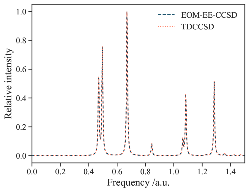
(a) H₂

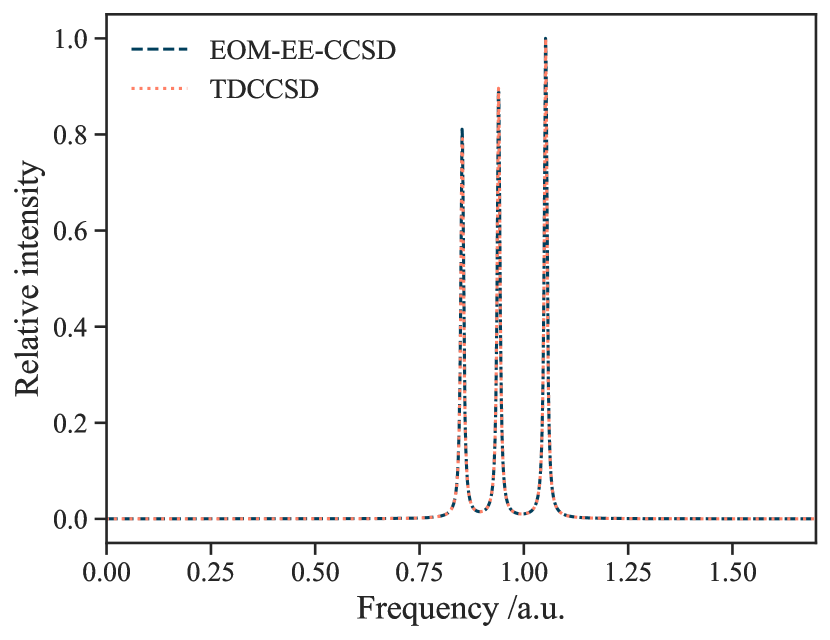
(b) He

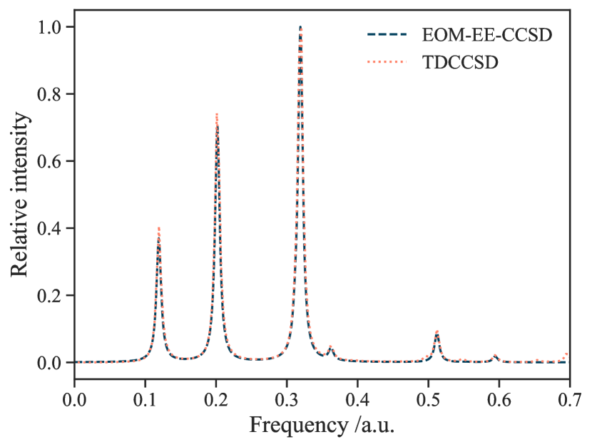
(c) Be

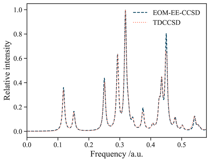
(d) LiH

Figure 1: Overlay of absorption spectra generated by TDCCSD and EOM-EE-CCSD at the magnetic-field strength $0.2\,\text{B}_{0}$ (along the internuclear axis for the diatomic molecules) with the aug-cc-pVTZ basis set.

III Results

III.1 Absorption Spectra

We have implemented the TDCC models discussed above in the open-source HyQD software [77] using the QUEST program [78] to generate optimized Hartree–Fock orbitals and Hamiltonian integrals in LAO basis to ensure magnetic gauge-origin invariance. [4] We validate our implementation of TDCCSD theory by comparing absorption spectra obtained from $\delta$-pulse simulations with spectra computed by the time-independent finite magnetic field EOM-EE-CCSD model [9] with the same LAO basis. The TDCCSD dipole moment is computed using the inherently real expectation-value functional proposed in Refs. 57, 79, and the electric-field strength is $\mathcal{E}=0.001\,\text{a.u.}$ While the excitation energies are identical with the two approaches, the intensities may differ when the number of electrons surpasses two. The approaches were nonetheless found to coincide quite well, with only slight deviations observed between EOM-EE-CCSD, TDCC and linear-response CC (LRCC) [10]. Although the time-dependent approach generates the full absorption spectrum, including core-valence excitations, we only compare low-lying transitions to avoid full diagonalization of the EOM-EE-CC matrix. The finite magnetic field EOM-EE-CCSD calculations are performed using the QCUMBRE software [80] together with an interface to the CFOUR program package, [81, 82] which provides the Hartree–Fock ground-state solution using the MINT integral package. [83] The EOM-EE-CCSD transition dipole moments are calculated with the expectation value approach. [74]

Absorption spectra are computed for H₂, He, Be, and LiH at the magnetic-field strength $0.2\,\text{B}_{0}$ directed along the $z$-axis, which coincides with the bond axis for the diatomic molecules. The geometries of H₂ and LiH are optimized in the magnetic field at the cTPSS level of theory with the aug-cc-pVDZ [84, 85, 86, 87] basis set using QUEST. [78, 42] The resulting bond lengths are $1.39106\,\text{a}_{0}$ for H₂ and $2.96117\,\text{a}_{0}$ for LiH.

For the EOM-EE-CCSD calculations, a convergence threshold of $10^{-7}$ is used for the Hartree–Fock densities and CC amplitudes, while a looser threshold of $10^{-6}$ ($10^{-5}$) is used for the right-hand (left-hand) side EOM vectors. For the TDCCSD simulations, a convergence threshold of $10^{-12}$ for the energy-gradient norm is used for the Hartree–Fock ground state optimization, while the CCSD ground-state amplitudes are converged to a residual norm of $10^{-12}$. The TDCCSD equations of motion are integrated using sixth order (three-stage, $s=3$) symplectic Gauss-Legendre integrator [88, 57] with time step $\Delta t=0.01\,\text{a.u.}$ and residual norm convergence criterion $10^{-10}$ for the implicit equations. The total simulation time is $1500\,\text{a.u.}$ for He and H₂, and $2000\,\text{a.u.}$ for Be and LiH.

Figure 1 displays the absorption spectra of the four systems obtained from the TDCCSD and EOM-EE-CCSD approaches with the aug-cc-pVTZ [84, 85, 86, 87] basis set. The excitation energies are equivalent to within the resolution of the FFT (approximately $0.004\,\text{a.u.}$ for He and H₂, and $0.003\,\text{a.u.}$ for Be and LiH) for all systems. For the two-electron systems, the intensities also agree, while minor deviations are observed for Be and LiH, as expected.

Corresponding absorption plots obtained from TDCC2 and EOM-EE-CC2/ EOM-EE-CCSD approaches can be found in the Supplementary material. No implementations of excitation energies for the OMP2 and NOCCD methods are available (only a pilot implementation of linear response theory was reported in Ref. 62), and, hence, no validation is possible for these methods.

III.2 Magnetic Optical Activity

III.2.1 Computational details

Magnetic optical activity calculations are performed for twenty magnetic-field strengths in the range $0\,\text{T}$ to $55\,000\,\text{T}$ by extracting the imaginary part of the polarizability as described in Sec. II.4. The field strength of the time-dependent electric field is chosen to be $\mathcal{E}=0.001\,\text{a.u.}$, which is small enough to warrant the dipole expansion in Eq. (21). We consider two cases: The orientation of the molecule is either taken to be independent of the direction of the magnetic field—i.e., the molecules of the sample are assumed to be randomly oriented—and the MOR is computed according to Eq. (1), or the molecule is taken to be fixed at the energetically most favorable orientation with respect to the magnetic-field direction and Eq. (4) is used. To determine the most favorable orientation, the Hartree–Fock/aug-cc-pVDZ ground-state bond lengths were computed at both the perpendicular and parallel orientation for each molecule. The ground-state energy difference as a function of the magnetic-field strength is displayed in Figure 2.

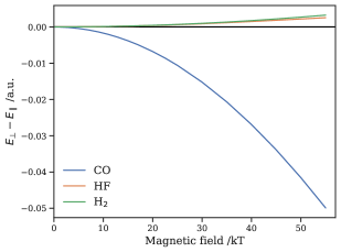
Figure 2: The Hartree–Fock/aug-cc-pVDZ ground-state energy difference between perpendicular and parallel molecular orientation with respect to the magnetic field direction as a function of field strength. The horizontal black line marks zero energy difference.

For H₂ and HF, the parallel orientation with respect to the magnetic field direction is the most energetically favorable, while the perpendicular orientation is found to be most favorable for CO. All three molecules are closed-shell diamagnetic molecules, and the difference in orientation stems from differences in the terms quadratic in the magnetic field—the diamagnetic terms—contained in Eq. (10). The optimized bond lengths for the three molecules can be found in the Supplementary Information.

When evaluating Eq. (1) and Eq. (4), the ideal gas approximation is employed at standard temperature ($0\,^{\circ}\text{C}$) and pressure ($1\,\text{atm}$). The number density thus is $\mathcal{N}=2.68678\times 10^{25}\,\text{m}^{-3}=3.98134\times 10^{-6}\,\text{a}_{0}^{-3}$, and

$$C=2.53048\times 10^{27}\,\frac{\text{J}\,\text{s}}{\text{C}^{2}\,\text{m}^{3}}=9.12748\times 10^{-8}\frac{\hbar}{\text{e}^{2}\,\text{a}_{0}^{3}}.$$ (23)

We compute the MOR for the H₂ molecule at $\omega=0.08284\,\text{a.u.}$ ($\lambda=550\,\text{nm}$), while $\omega=0.11391\,\text{a.u.}$ ($\lambda=400\,\text{nm}$) is used for the CO and HF molecules in accordance with the experimental work of Ingersoll and Lebenberg. [89]

For the randomly oriented case, simulations are carried with experimental field-free bond lengths: $1.4\,\text{a}_{0}$ for H₂, $2.132\,\text{a}_{0}$ for CO, and $1.7328\,\text{a}_{0}$ for HF. For the fixed orientation case, the bond lengths of H₂, CO, and HF are optimized for each magnetic-field strength at the cTPSS/aug-cc-pVDZ level of theory with the magnetic field vector parallel (H₂ and HF) or perpendicular (CO) to the bond axis.

We compute the MOR from TDHF, TDCC2, TDCCSD, TDOMP2, and TDNOCCD simulations with the HyQD software. [77] Apart from using a stricter residual norm convergence criteria of $10^{-12}$ for the implicit equations of the Gauss-Legendre integrator, the same convergence thresholds are applied for the MOR calculations as those specified in Sec. III.1 The TDCDFT simulations are performed with the current–dependent exchange–correlation functionals cTPSS, cTPSSh, and cTPSSrsh as described in Ref. 40. The density is propagated using the Magnus 2 propagator [90] with a modest time step of $0.1\,\text{a.u.}$, which has been shown to yield a good balance between accuracy and efficiency for computing absorption spectra in the presence of a magnetic field. [40] The TDCDFT simulations are performed with the QUEST code. [78] For all calculations, the aug-cc-pVDZ basis set is employed, and it should be noted that the basis set limit has not been reached. [37] Moreover, the CC expansion lacks triple excitations, which are important for high accuracy, [38] and rovibrational effects are not taken into account. Consequently, the simulations presented here cannot be expected to reproduce or predict experimental results with very high accuracy.

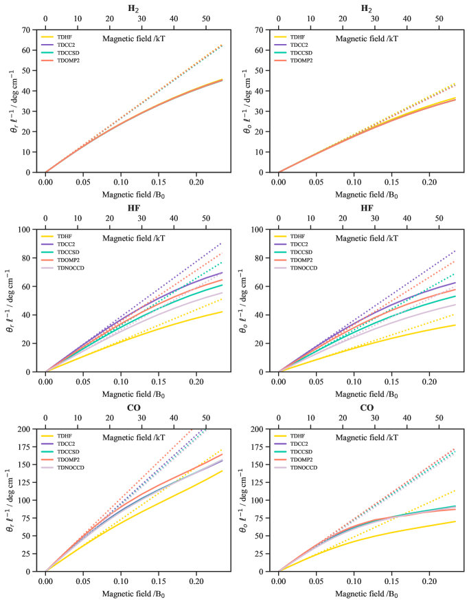
Figure 3: The magnetic optical rotation of H₂, HF, and CO as a function of the magnetic-field strength computed with wave function methods. The panels on the left display the MOR for the randomly oriented molecules, while the panels on the right display the MOR for the fixed orientation relative to the magnetic field vector (parallel for H₂ and HF systems, perpendicular for CO). The dashed lines are obtained from the Verdet constants in Table 1.

III.2.2 Verdet constants

We determine Verdet constants by fitting the MOR data for randomly oriented samples to a fifth-order polynomial in the magnetic-field strength, identifying $V(\omega)$ as the coefficient of the linear term. The results are listed in Table 1 along with the experimental results of Ingersoll and Lebenberg. [89]

Table 1: The Verdet constant (in $10^{-7}\,\text{a.u.}$) extracted from simulations. Experimental values are taken from Ref. 89.

	H2	HF	CO
$\omega/\text{a.u.}$	0.08284	0.11391	0.11391
TDHF	0.248	0.202	0.687
TDCC2	0.246	0.358	0.906
TDCCSD	0.245	0.304	0.884
TDOMP2	0.247	0.329	0.972
TDNOCCD	-	0.274	0.876
cTPSS	0.303	0.416	0.987
cTPSSh	0.235	0.288	0.761
cTPSSrsh	0.160	0.202	0.512
Exp.	0.251	-	0.895

While electron correlation effects are important for HF and CO, their impact is less pronounced in the case of H₂. The wave function methods that take electron correlation into account yield Verdet constant which agree with experimental values (for H₂ and CO) to within $2$–$10\%$, which is reasonable considering the lack of higher-order correlation effects [38] and vibrational contributions, [91] in addition to the relatively small basis set. With errors ranging from $6\%$ to $38\%$, the TDCDFT model with the cTPSSrsh functional exhibit comparatively large errors, especially considering that the TDHF results remain below $24\%$.

Computations conducted using quadratic response theory [41, 37] should yield identical Verdet constants, although slight variations may arise, for example, due to numerical errors from the finite-difference calculations involved in the linear-response-function extraction. [75, 76] Parkinson et al. [41] computed Verdet constants for the three molecules at the Hartree–Fock level (i.e., the random phase approximation). They used a somewhat larger basis set than aug-cc-pVDZ, albeit without the LAO phase factors, and obtained Verdet constants of $0.232\times 10^{-7}\,\text{a.u.}$ for H₂, $0.219\times 10^{-7}\,\text{a.u.}$ for HF, and $0.702\times 10^{-7}\,\text{a.u.}$ for CO, in fair agreement with our TDHF results in Table 1. Coriani et al. [37] computed the Verdet constant for HF at the CCSD level with the same basis set to be $0.3038\times 10^{-7}\,\text{a.u.}$, which is within $0.03\%$ of our result ($0.3037\times 10^{-7}\,\text{a.u.}$). This confirms that our MOR procedure indeed reproduces quadratic response theory at low magnetic-field strengths.

III.2.3 TDCC results at finite magnetic field

Figure 3 shows the MOR obtained from wave function-based simulations of H₂, HF, and CO as a function of magnetic-field strength, with the dashed lines representing the values predicted from Eq. (3) using the Verdet constants reported in Table 1. Results for randomly oriented molecules are shown in the left-hand panels, while those for oriented molecules are shown in the right-hand panels. There are significant deviations from linearity for both oriented and randomly oriented samples, as we shall discuss in more detail below.

The two uppermost panels of Fig. 3 show the MOR of H₂ obtained from TDHF, TDCC2, TDCCSD, and TDOMP2 simulations. Since the H₂ molecule is a two-electron system, the TDCCSD and TDNOCCD methods are equivalent. As also observed for the Verdet constants above, electron correlation effects are not highly important for the MOR of H₂ at the range of magnetic-field strengths considered here. The effect of orientation—which includes varying bond lengths—is significant, with $\theta_{r}$ roughly $28\%$ greater than $\theta_{o}$.

For both HF and CO, however, correlation effects are crucial, confirming previous observations based on quadratic response theory by Parkinson et al. [41] and Coriani et al. [38] While the TDCCSD and TDNOCCD results agree for CO, the optimization of the time-dependent orbitals in the TDNOCCD method give rise to a significant change compared with the static orbitals of TDCCSD theory for the HF molecule. This observation also applies to the second-order approximations TDCC2 and TDOMP2, where we also note that TDOMP2 results are closer to the TDCCSD ones than those obtained from TDCC2 theory for HF. However, this is not at all the case for CO. The latter is in agreement with magnetic field-free polarizability and hyperpolarizability results reported by Kristiansen et al. [59] It is, however, not possible to conclude which of the TDNOCCD and TDCCSD methods is superior based on the present results, as it requires a more careful study of convergence with respect to higher-order excitations beyond doubles. We will, therefore, compare TDCDFT results with the MOR obtained from both the TDCCSD and TDNOCCD methods.

It is noteworthy that the MOR is almost identical for oriented and randomly oriented HF, whereas a significant orientation effect is observed for the CO molecule. While one might speculate that the “oriented” contribution, Eq. (4), dominates the averaging in Eq. (1) for HF, it turns out to be caused by the change in bond length obtained in the magnetic-field dependent geometry optimization.

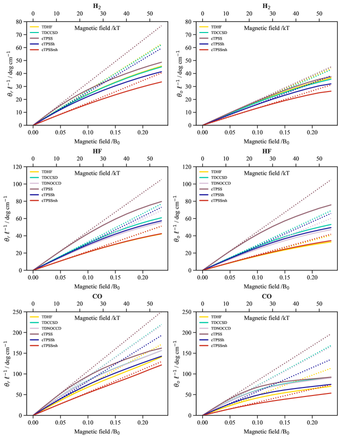
Figure 4: The magnetic optical rotation of H₂, HF, and CO as a function of the magnetic-field strength computed with TDCDFT and the TDHF, TDCCSD, and TDNOCCD methods. The panels on the left display the MOR for the randomly oriented molecules, while the panels on the right display the MOR for the fixed orientation relative to the magnetic field vector (parallel for H₂ and HF systems, perpendicular for CO). The dashed lines are obtained from the Verdet constants in Table 1.

III.2.4 TDCDFT results at finite magnetic field

Figure 4 shows the MOR obtained from TDCDFT simulations of H₂, HF, and CO as a function of magnetic-field strength with the dashed lines representing the predicted values using Eq. (3) with the Verdet constants reported in Table 1. Results for randomly oriented and oriented molecules are shown in the left- and right-hand panels, respectively, and the TDHF, TDCCSD, and TDNOCCD results are reproduced here for comparison. Also for the TDCDFT methods, we observe significant deviations from linearity as the magnetic-field strength increases.

The cTPSSh and cTPSSrsh functionals have previously been applied to the calculation of isotropic NMR shielding constants, [73] where no significant improvements were found compared with the cTPSS functional. The cTPSSrsh functional has, however, been found to better describe excited states compared to cTPSS and cTPSSh in the magnetic field-free case. [40] We observe that the cTPSSh functional generally produces MOR values that are somewhat closer to TDCCSD/TDNOOCD results than the cTPSS functional, Moreover, the cTPSSh functional outperforms the TDHF method for HF, and CO, but not for H₂. The MOR values computed using the cTPSSh functional fall in between the cTPSS and cTPSSrsh results, which are over- and under-estimates of the MOR, respectively. The poor performance of the cTPSSrsh functional is somewhat surprising considering that range separation is known to improve the description of nonlinear properties.[92, 93] The cTPSSrsh functional incorporates a large fraction of the current-independent PBE functional, which might contribute to the quite poor performance in finite magnetic fields. When the magnetic field is set to zero, the cTPSSrsh functional yields ground state energies and dipole moments comparable to cTPSSh, both of which outperform the cTPSS functional.

III.2.5 Deviation from Verdet’s linear law

Table 2: The magnetic-field strength (in kT) at which the nonperturbative MOR deviates from Verdet’s law by a chosen percentage.

		Orientation
		Random		Fixed
		3%	5%	3%	5%
H2	TDHF	9.03	13.1	22.1	28.5
	TDCC2	9.14	13.2	21.9	28.2
	TDCCSD	9.25	13.3	21.6	27.8
	TDOMP2	9.03	13.0	21.9	28.2
	cTPSS	6.39	9.69	27.1	32.3
	cTPSSh	7.76	11.5	29.1	34.0
	cTPSSrsh	16.2	22.6	31.2	36.2
HF	TDHF	20.3	26.4	18.7	24.4
	TDCC2	17.1	22.1	15.4	20.0
	TDCCSD	18.7	24.0	16.2	21.3
	TDOMP2	17.5	22.6	15.1	19.5
	TDNOCCD	19.3	24.7	18.3	23.2
	cTPSS	16.9	21.4	15.2	19.3
	cTPSSh	18.1	23.3	13.3	18.6
	cTPSSrsh	21.2	27.4	18.2	24.4
CO	TDHF	14.9	19.0	11.6	14.2
	TDCC2	12.4	15.4	10.7	12.9
	TDCCSD	12.8	16.0	11.0	13.3
	TDOMP2	11.5	14.5	10.2	11.4
	TDNOCCD	12.7	15.9	11.0	13.3
	cTPSS	13.7	16.2	9.86	11.9
	cTPSSh	11.0	14.6	11.1	13.4
	cTPSSrsh	24.9	33.3	13.9	17.0

As noted above, it is evident from Figs. 3 and 4 that Verdet’s linear relation between the MOR and the magnetic-field strength only holds for sufficiently small magnetic-field strengths. While this is not surprising, considering that the observations of Verdet can be accounted for by first-order perturbation theory, it is not straightforward to uniquely define a field strength at which linearity is broken. In this work, we will define the “breaking point” as the magnetic-field strength at which the fifth-order polynomial function fitted to the nonperturbative MOR deviates from the value predicted from the Verdet constants, defined as the linear coefficient of this polynomial function, by a given percentage.

The magnetic-field strengths at which $3\%$ and $5\%$ deviations are observed can be found in Table 2. With random orientation, the breaking point roughly lies somewhere between $10$ and $20\,\text{kT}$ ($0.04$–$0.09\,\text{B}_{0}$), $2$–$3$ orders of magnitude above the strongest sustainable static magnetic-field strength produced on Earth with a high-temperature superconducting magnet, namely $45.5\,\text{T}$ ($2\times 10^{-4}\,\text{B}_{0}$). [94] At $45.5\,\text{T}$, the TDCCSD and TDNOCCD results deviate from linearity by about $0.9\%$ for H₂ and CO and by about $0.09\%$ for HF (with random orientation). Not surprisingly, our results thus indicate that Verdet’s law can be safely applied for the range of magnetic-field strengths that can be produced in experimental setups.

IV Concluding remarks

We have in this work presented the first implementation of TDCC theory for the study of laser-driven multi-electron dynamics in finite magnetic fields. The implementation is validated by comparing linear absorption spectra obtained from simulations with those obtained from time-independent EOM-EE-CC theory. The implementation supports both static and dynamic reference determinants with the orbitals expanded in London atomic orbitals to ensure magnetic gauge-origin invariance.

The new implementation is applied to the calculation of magnetic optical rotation at finite magnetic-field strengths, demonstrating that Verdet’s linear relationship is valid up to field strengths of roughly $10$–$20\,\text{kT}$ ($0.04$–$0.09\,\text{B}_{0}$). A deviation from linearity below $1\%$ is found at $45.5\,\text{T}$, which is the strongest sustainable static magnetic field ever produced by a superconducting magnet on Earth. We have also compared the TDCC magnetic optical rotations with those obtained from TDCDFT simulations using the current-dependent cTPSS, cTPSSh, and cTPSSrsh density-functional approximations. With TDCCSD and TDNOCCD results as benchmark, we find that the best-performing functional is cTPSSh. The cTPSS functional tends to overestimate the rotation while the cTPSSrsh functional tends to underestimate it.

Supplementary material

The supplementary material contains cTPSS/aug-cc-pVDZ equilibrium bond lengths of H₂, HF, and CO placed in a magnetic field parallel or perpendicular to the bond axis with field strengths ranging from $1\,\text{T}$ to $55\,\text{kT}$. The overlayed absorption spectra generated from TDCC2 simulations and from time-independent EOM-EE-CC2 calculations can also be found in the supplementary material.

Data availability statement

The data that support the findings of this study are available from the corresponding author upon reasonable request.

References

- Lange et al. [2012] K. K. Lange, E. I. Tellgren, M. R. Hoffmann, and T. Helgaker, “A Paramagnetic Bonding Mechanism for Diatomics in Strong Magnetic Fields,” Science 337, 327–331 (2012).
- Lewenstein et al. [1994] M. Lewenstein, P. Balcou, M. Y. Ivanov, A. L’Huillier, and P. B. Corkum, “Theory of high-harmonic generation by low-frequency laser fields,” Phys. Rev. A 49, 2117–2132 (1994).
- Hollands et al. [2023] M. A. Hollands, S. Stopkowicz, M. P. Kitsaras, F. Hampe, S. Blaschke, and J. J. Hermes, “A DZ white dwarf with a magnetic field,” Mon. Notices Royal Astron. Soc. 520, 3560–3575 (2023).
- Tellgren, Soncini, and Helgaker [2008] E. I. Tellgren, A. Soncini, and T. Helgaker, “Nonperturbative ab initio calculations in strong magnetic fields using London orbitals,” J. Chem. Phys. 129, 154114 (2008).
- Sen, Lange, and Tellgren [2019] S. Sen, K. K. Lange, and E. I. Tellgren, “Excited States of Molecules in Strong Uniform and Nonuniform Magnetic Fields,” J. Chem. Theory Comput. 15, 3974–3990 (2019).
- Sun, Williams-Young, and Li [2019] S. Sun, D. Williams-Young, and X. Li, “An ab Initio Linear Response Method for Computing Magnetic Circular Dichroism Spectra with Nonperturbative Treatment of Magnetic Field,” J. Chem. Theory Comput. 15, 3162–3169 (2019).
- Sun et al. [2019] S. Sun, D. B. Williams-Young, T. F. Stetina, and X. Li, “Generalized Hartree–Fock with Nonperturbative Treatment of Strong Magnetic Fields: Application to Molecular Spin Phase Transitions,” J. Chem. Theory Comput. 15, 348–356 (2019).
- Stopkowicz et al. [2015] S. Stopkowicz, J. Gauss, K. K. Lange, E. I. Tellgren, and T. Helgaker, “Coupled-cluster theory for atoms and molecules in strong magnetic fields,” J. Chem. Phys. 143, 074110 (2015).
- Hampe and Stopkowicz [2017] F. Hampe and S. Stopkowicz, “Equation-of-motion coupled-cluster methods for atoms and molecules in strong magnetic fields,” J. Chem. Phys. 146, 154105 (2017).
- Hampe and Stopkowicz [2019] F. Hampe and S. Stopkowicz, “Transition-Dipole Moments for Electronic Excitations in Strong Magnetic Fields Using Equation-of-Motion and Linear Response Coupled-Cluster Theory,” Journal of Chemical Theory and Computation 15, 4036–4043 (2019).
- Hampe, Gross, and Stopkowicz [2020] F. Hampe, N. Gross, and S. Stopkowicz, “Full triples contribution in coupled-cluster and equation-of-motion coupled-cluster methods for atoms and molecules in strong magnetic fields,” Phys. Chem. Chem. Phys. 22, 23522–23529 (2020).
- Vignale and Rasolt [1987] G. Vignale and M. Rasolt, “Density-functional theory in strong magnetic fields,” Phys. Rev. Lett. 59, 2360–2363 (1987).
- Vignale and Rasolt [1988] G. Vignale and M. Rasolt, “Current- and spin-density-functional theory for inhomogeneous electronic systems in strong magnetic fields,” Phys. Rev. B 37, 10685–10696 (1988).
- Tellgren et al. [2012] E. I. Tellgren, S. Kvaal, E. Sagvolden, U. Ekström, A. M. Teale, and T. Helgaker, “Choice of basic variables in current-density-functional theory,” Phys. Rev. A 86, 062506 (2012).
- Tellgren et al. [2014] E. I. Tellgren, A. M. Teale, J. W. Furness, K. K. Lange, U. Ekström, and T. Helgaker, “Non-perturbative calculation of molecular magnetic properties within current-density functional theory,” J. Chem. Phys. 140, 034101 (2014).
- Furness et al. [2015] J. W. Furness, J. Verbeke, E. I. Tellgren, S. Stopkowicz, U. Ekström, T. Helgaker, and A. M. Teale, “Current Density Functional Theory Using Meta-Generalized Gradient Exchange-Correlation Functionals,” J. Chem. Theory Comput. 11, 4169–4181 (2015).
- Kvaal et al. [2021] S. Kvaal, A. Laestadius, E. Tellgren, and T. Helgaker, “Lower Semicontinuity of the Universal Functional in Paramagnetic Current–Density Functional Theory,” J. Phys. Chem. Lett. 12, 1421–1425 (2021).
- Goings, Lestrange, and Li [2018] J. J. Goings, P. J. Lestrange, and X. Li, “Real-time time-dependent electronic structure theory,” WIREs Comput. Mol. Sci. 8, e1341 (2018).
- Li et al. [2020] X. Li, N. Govind, C. Isborn, A. E. DePrince, and K. Lopata, “Real-Time Time-Dependent Electronic Structure Theory,” Chem. Rev. 120, 9951–9993 (2020).
- Nisoli et al. [2017] M. Nisoli, P. Decleva, F. Calegari, A. Palacios, and F. Martín, “Attosecond Electron Dynamics in Molecules,” Chem. Rev. 117, 10760–10825 (2017).
- Palacios and Martín [2020] A. Palacios and F. Martín, “The quantum chemistry of attosecond molecular science,” WIREs Comput. Mol. Sci. 10, e1430 (2020).
- Faraday [1846] M. Faraday, “I. Experimental researches in electricity.—Nineteenth series,” Philos. Trans. R. Soc. London 136, 1–20 (1846).
- Buckingham and Stephens [1966] A. D. Buckingham and P. J. Stephens, “Magnetic Optical Activity,” Ann. Rev. Phys. Chem. 17, 399–432 (1966).
- Knudsen [1976] O. Knudsen, “The Faraday Effect and Physical Theory, 1845-1873,” Arch. Hist. Exact Sci. 15, 235–281 (1976).
- Hui and O’Sullivan [2023] R. Hui and M. O’Sullivan, “Fiber-based optical metrology and spectroscopy techniques,” in Fiber-Optic Measurement Techniques, edited by R. Hui and M. O’Sullivan (Academic Press, Boston, MA, 2023) 2nd ed., pp. 557–649.
- Iida and Wakana [2003] T. Iida and H. Wakana, “Communications Satellite Systems,” in Encyclopedia of Physical Science and Technology, edited by R. A. Meyers (Academic Press, New York, 2003) 3rd ed., pp. 375–408.
- Han [2017] J. L. Han, “Observing Interstellar and Intergalactic Magnetic Fields,” Annu. Rev. Astron. Astrophys. 55, 111–157 (2017).
- Carothers, Norwood, and Pyun [2022] K. J. Carothers, R. A. Norwood, and J. Pyun, “High Verdet Constant Materials for Magneto-Optical Faraday Rotation: A Review,” Chem. Mater. 34, 2531–2544 (2022).
- Verdet [1854] E. Verdet, “Recherches sur les propriétés optiques développées dans les corps transparents par l’action du magnétisme,” Ann. Chim. Phys. Sér. 41, 370–412 (1854).
- Verdet [1855] E. Verdet, “Recherches sur les propriétés optiques développées dans les corps transparents par l’action du magnétisme,” Ann. Chim. Phys. Sér. 43, 37–44 (1855).
- Verdet [1858] E. Verdet, “Recherches sur les propriétés optiques développées dans les corps transparents par l’action du magnétisme,” Ann. Chim. Phys. Sér. 52, 129–163 (1858).
- Verdet [1863] E. Verdet, “Recherches sur les propriétés optiques développées dans les corps transparents par l’action du magnétisme. de la dispersion des plans de polarisations des rayons de diverses couleurs",” Ann. Chim. Phys. Sér. 69, 415–491 (1863).
- Serber [1932] R. Serber, “The Theory of the Faraday Effect in Molecules,” Phys. Rev. 41, 489–506 (1932).
- Barron [2004] L. D. Barron, Molecular Light Scattering and Optical Activity, 2nd ed. (Cambridge University Press, Cambridge, 2004).
- Parkinson and Oddershede [1997] W. A. Parkinson and J. Oddershede, “Response function analysis of magnetic optical rotation,” Int. J. Quantum Chem. 64, 599–605 (1997).
- Coriani et al. [1997] S. Coriani, C. Hättig, P. Jørgensen, A. Halkier, and A. Rizzo, “Coupled cluster calculations of Verdet constants,” Chem. Phys. Lett. 281, 445–451 (1997).
- Coriani et al. [2000a] S. Coriani, C. Hättig, P. Jørgensen, and T. Helgaker, “Gauge-origin independent magneto-optical activity within coupled cluster response theory,” J. Chem. Phys. 113, 3561–3572 (2000a).
- Coriani et al. [2000b] S. Coriani, P. Jørgensen, O. Christiansen, and J. Gauss, “Triple excitation effects in coupled cluster calculations of Verdet constants,” Chem. Phys. Lett. 330, 463–470 (2000b).
- Ofstad et al. [2023a] B. S. Ofstad, E. Aurbakken, Ø. S. Schøyen, H. E. Kristiansen, S. Kvaal, and T. B. Pedersen, “Time-dependent coupled-cluster theory,” WIREs Comput. Mol. Sci. , e1666 (2023a), in press; available online.
- Wibowo, Irons, and Teale [2021] M. Wibowo, T. J. P. Irons, and A. M. Teale, “Modeling Ultrafast Electron Dynamics in Strong Magnetic Fields Using Real-Time Time-Dependent Electronic Structure Methods,” J. Chem. Theory Comput. 17, 2137–2165 (2021).
- Parkinson et al. [1993] W. A. Parkinson, S. P. A. Sauer, J. Oddershede, and D. M. Bishop, “Calculation of the Verdet constants for H2, N2, CO, and FH,” J. Chem. Phys. 98, 487–495 (1993).
- Irons, David, and Teale [2021] T. J. P. Irons, G. David, and A. M. Teale, “Optimizing Molecular Geometries in Strong Magnetic Fields,” J. Chem. Theory Comput. 17, 2166–2185 (2021).
- Bishop and Cybulski [1990] D. M. Bishop and S. M. Cybulski, “Magnetic optical rotation in H2 and D2,” J. Chem. Phys. 93, 590–599 (1990).
- London [1937] F. London, “Théorie quantique des courants interatomiques dans les combinaisons aromatiques,” J. Phys. Radium 8, 397–409 (1937).
- Schmelcher and Cederbaum [1988] P. Schmelcher and L. S. Cederbaum, “Molecules in strong magnetic fields: Properties of atomic orbitals,” Phys. Rev. A 37, 672–681 (1988).
- Lehtola, Dimitrova, and Sundholm [2020] S. Lehtola, M. Dimitrova, and D. Sundholm, “Fully numerical electronic structure calculations on diatomic molecules in weak to strong magnetic fields,” Mol. Phys. 118, e1597989 (2020).
- Helgaker, Jørgensen, and Olsen [2000] T. Helgaker, P. Jørgensen, and J. Olsen, Molecular Electronic-Structure Theory (John Wiley & Sons, Chichester, 2000).
- Crawford and Schaefer III [2000] T. D. Crawford and H. F. Schaefer III, “An Introduction to Coupled Cluster Theory for Computational Chemists,” in Reviews in Computational Chemistry, Vol. 14, edited by K. B. Lipkowitz and D. B. Boyd (John Wiley & Sons, New York, 2000) pp. 33–136.
- Bartlett and Musiał [2007] R. J. Bartlett and M. Musiał, “Coupled-cluster theory in quantum chemistry,” Rev. Mod. Phys. 79, 291–352 (2007).
- Shavitt and Bartlett [2009] I. Shavitt and R. J. Bartlett, Many-Body Methods in Chemistry and Physics. MBPT and Coupled-Cluster Theory (Cambridge University Press, New York, 2009).
- Krylov [2008] A. I. Krylov, “Equation-of-Motion Coupled-Cluster Methods for Open-Shell and Electronically Excited Species: The Hitchhiker’s Guide to Fock Space,” Annu. Rev. Phys. Chem. 59, 433–462 (2008).
- Sneskov and Christiansen [2012] K. Sneskov and O. Christiansen, “Excited state coupled cluster methods,” WIREs Comput. Mol. Sci. 2, 566–584 (2012).
- Helgaker et al. [2012] T. Helgaker, S. Coriani, P. Jørgensen, K. Kristensen, J. Olsen, and K. Ruud, “Recent Advances in Wave Function-Based Methods of Molecular-Property Calculations,” Chem. Rev. 112, 543–631 (2012).
- Raghavachari et al. [1989] K. Raghavachari, G. W. Trucks, J. A. Pople, and M. Head-Gordon, “A fifth-order perturbation comparison of electron correlation theories,” Chem. Phys. Lett. 157, 479–483 (1989).
- Tellgren, Reine, and Helgaker [2012] E. I. Tellgren, S. S. Reine, and T. Helgaker, “Analytical GIAO and hybrid-basis integral derivatives: application to geometry optimization of molecules in strong magnetic fields,” Phys. Chem. Chem. Phys. 14, 9492–9499 (2012).
- Irons, Zemen, and Teale [2017] T. J. P. Irons, J. Zemen, and A. M. Teale, “Efficient Calculation of Molecular Integrals over London Atomic Orbitals,” J. Chem. Theory Comput. 13, 3636–3649 (2017).
- Pedersen and Kvaal [2019] T. B. Pedersen and S. Kvaal, “Symplectic integration and physical interpretation of time-dependent coupled-cluster theory,” J. Chem. Phys. 150, 144106 (2019).
- Christiansen, Koch, and Jørgensen [1995] O. Christiansen, H. Koch, and P. Jørgensen, “The second-order approximate coupled cluster singles and doubles model CC2,” Chem. Phys. Lett. 243, 409–418 (1995).
- Kristiansen et al. [2022] H. E. Kristiansen, B. S. Ofstad, E. Hauge, E. Aurbakken, Ø. S. Schøyen, S. Kvaal, and T. B. Pedersen, “Linear and Nonlinear Optical Properties from TDOMP2 Theory,” J. Chem. Theory Comput. 18, 3687–3702 (2022).
- Pedersen, Koch, and Hättig [1999] T. B. Pedersen, H. Koch, and C. Hättig, “Gauge invariant coupled cluster response theory,” J. Chem. Phys. 110, 8318–8327 (1999).
- Sato et al. [2018] T. Sato, H. Pathak, Y. Orimo, and K. L. Ishikawa, “Communication: Time-dependent optimized coupled-cluster method for multielectron dynamics,” J. Chem. Phys. 148, 051101 (2018).
- Pedersen, Fernández, and Koch [2001] T. B. Pedersen, B. Fernández, and H. Koch, “Gauge invariant coupled cluster response theory using optimized nonorthogonal orbitals,” J. Chem. Phys. 114, 6983–6993 (2001).
- Kvaal [2012] S. Kvaal, “Ab initio quantum dynamics using coupled-cluster,” J. Chem. Phys. 136, 194109 (2012).
- Kristiansen et al. [2020] H. E. Kristiansen, Ø. S. Schøyen, S. Kvaal, and T. B. Pedersen, “Numerical stability of time-dependent coupled-cluster methods for many-electron dynamics in intense laser pulses,” J. Chem. Phys. 152, 071102 (2020).
- Pathak, Sato, and Ishikawa [2020] H. Pathak, T. Sato, and K. L. Ishikawa, “Time-dependent optimized coupled-cluster method for multielectron dynamics. III. A second-order many-body perturbation approximation,” J. Chem. Phys. 153, 034110 (2020).
- Lieb [1983] E. H. Lieb, “Density functionals for Coulomb systems,” Int. J. Quantum Chem. 24, 243–277 (1983).
- Lee, Handy, and Colwell [1995] A. M. Lee, N. C. Handy, and S. M. Colwell, “The density functional calculation of nuclear shielding constants using London atomic orbitals,” J. Chem. Phys. 103, 10095–10109 (1995).
- Zhu and Trickey [2006] W. Zhu and S. B. Trickey, “Exact density functionals for two-electron systems in an external magnetic field,” J. Chem. Phys. 125, 094317 (2006).
- Dobson [1993] J. F. Dobson, “Alternative expressions for the fermi hole curvature,” J. Chem. Phys. 98, 8870–8872 (1993).
- Becke [1996] A. D. Becke, “Current-density dependent exchange-correlation functionals,” Can. J. Chem. 74, 995–997 (1996).
- Bates and Furche [2012] J. E. Bates and F. Furche, “Harnessing the meta-generalized gradient approximation for time-dependent density functional theory,” J. Chem. Phys. 137, 164105 (2012).
- Tao et al. [2003] J. Tao, J. P. Perdew, V. N. Staroverov, and G. E. Scuseria, “Climbing the density functional ladder: Nonempirical meta–generalized gradient approximation designed for molecules and solids,” Phys. Rev. Lett. 91, 146401 (2003).
- Irons et al. [2020] T. J. P. Irons, L. Spence, G. David, B. T. Speake, T. Helgaker, and A. M. Teale, “Analyzing Magnetically Induced Currents in Molecular Systems Using Current-Density-Functional Theory,” J. Phys. Chem. A 124, 1321–1333 (2020).
- Stanton and Bartlett [1993] J. F. Stanton and R. J. Bartlett, “The equation of motion coupled-cluster method. A systematic biorthogonal approach to molecular excitation energies, transition probabilities, and excited state properties,” J. Chem. Phys. 98, 7029–7039 (1993).
- Ding et al. [2013] F. Ding, B. E. Van Kuiken, B. E. Eichinger, and X. Li, “An efficient method for calculating dynamical hyperpolarizabilities using real-time time-dependent density functional theory,” J. Chem. Phys. 138, 064104 (2013).
- Ofstad et al. [2023b] B. S. Ofstad, H. E. Kristiansen, E. Aurbakken, Ø. S. Schøyen, S. Kvaal, and T. B. Pedersen, “Adiabatic extraction of nonlinear optical properties from real-time time-dependent electronic-structure theory,” J. Chem. Phys. 158, 154102 (2023b).
- Aurbakken, E. and Fredly, K. H. and Kristiansen, H. E. and Kvaal, S. and Myhre, R. H. and Ofstad, B. S. and Pedersen, T. B. and Schøyen, Ø. S. and Sutterud, H. and Winther-Larsen, S. G. [2 04] Aurbakken, E. and Fredly, K. H. and Kristiansen, H. E. and Kvaal, S. and Myhre, R. H. and Ofstad, B. S. and Pedersen, T. B. and Schøyen, Ø. S. and Sutterud, H. and Winther-Larsen, S. G., “HyQD: Hylleraas Quantum Dynamics,” (2023-02-04), URL: https://github.com/HyQD.
- QUEST [2022] QUEST, “QUEST, a rapid development platform for QUantum Electronic-Structure Techniques,” (2022), URL: https://quest.codes.
- Pedersen and Koch [1997] T. B. Pedersen and H. Koch, “Coupled cluster response functions revisited,” J. Chem. Phys. 106, 8059–8072 (1997).
- Hampe et al. [2023] F. Hampe, S. Stopkowicz, N. Gross, M.-P. Kitsaras, L. Grazioli, S. Blaschke, P. Yergün, and L. Monzel, “QCUMBRE, quantum chemical utility enabling magnetic-field dependent investigations benefitting from rigorous electron-correlation treatment,” (2023).
- [81] J. F. Stanton, J. Gauss, L. Cheng, M. E. Harding, D. A. Matthews, and P. G. Szalay, “CFOUR, Coupled-Cluster techniques for Computational Chemistry, a quantum-chemical program package,” With contributions from A. Asthana, A.A. Auer, R.J. Bartlett, U. Benedikt, C. Berger, D.E. Bernholdt, S. Blaschke, Y. J. Bomble, S. Burger, O. Christiansen, D. Datta, F. Engel, R. Faber, J. Greiner, M. Heckert, O. Heun, M. Hilgenberg, C. Huber, T.-C. Jagau, D. Jonsson, J. Jusélius, T. Kirsch, M.-P. Kitsaras, K. Klein, G.M. Kopper, W.J. Lauderdale, F. Lipparini, J. Liu, T. Metzroth, L.A. Mück, D.P. O’Neill, T. Nottoli, J. Oswald, D.R. Price, E. Prochnow, C. Puzzarini, K. Ruud, F. Schiffmann, W. Schwalbach, C. Simmons, S. Stopkowicz, A. Tajti, T. Uhlirova, J. Vázquez, F. Wang, J.D. Watts, P. Yergün. C. Zhang, XZheng, and the integral packages MOLECULE (J. Almlöf and P.R. Taylor), PROPS (P.R. Taylor), ABACUS (T. Helgaker, H.J. Aa. Jensen, P. Jørgensen, and J. Olsen), and ECP routines by A. V. Mitin and C. van Wüllen. For the current version, see http://www.cfour.de.
- Matthews et al. [2020] D. A. Matthews, L. Cheng, M. E. Harding, F. Lipparini, S. Stopkowicz, T.-C. Jagau, P. G. Szalay, J. Gauss, and J. F. Stanton, “Coupled-cluster techniques for computational chemistry: The CFOUR program package,” J. Chem. Phys. 152, 214108 (2020).
- Gauss et al. [2021] J. Gauss, F. Lipparini, S. Burger, S. Blaschke, M. Kitsaras, and S. Stopkowicz, “MINT, Mainz INTegral package,” (2015-2021), Johannes Gutenberg-Universität Mainz, unpublished.
- Dunning [1989] T. H. Dunning, “Gaussian basis sets for use in correlated molecular calculations. I. The atoms boron through neon and hydrogen,” J. Chem. Phys. 90, 1007–1023 (1989).
- Kendall, Dunning, and Harrison [1992] R. A. Kendall, T. H. Dunning, and R. J. Harrison, “Electron affinities of the first-row atoms revisited. Systematic basis sets and wave functions,” J. Chem. Phys. 96, 6796–6806 (1992).
- Woon and Dunning [1994] D. E. Woon and T. H. Dunning, “Gaussian basis sets for use in correlated molecular calculations. iv. calculation of static electrical response properties,” J. Chem. Phys. 100, 2975–2988 (1994).
- Prascher et al. [2011] B. P. Prascher, D. E. Woon, K. A. Peterson, T. H. Dunning, and A. K. Wilson, “Gaussian basis sets for use in correlated molecular calculations. vii. valence, core-valence, and scalar relativistic basis sets for li, be, na, and mg,” Theor. Chem. Acc. 128, 69–82 (2011).
- Hairer, Wanner, and Lubich [2006] E. Hairer, G. Wanner, and C. Lubich, Geometric Numerical Integration, 2nd ed. (Springer, Berlin, Heidelberg, 2006).
- Ingersoll and Lebenberg [1956] L. R. Ingersoll and D. H. Lebenberg, “Faraday Effect in Gases and Vapors. II,” J. Opt. Soc. Am. 46, 538–542 (1956).
- Blanes and Casas [2016] S. Blanes and F. Casas, A Concise Introduction to Geometric Numerical Integration (CRC press: Boca Raton, 2016).
- Mort and Autschbach [2007] B. C. Mort and J. Autschbach, “Vibrational corrections to magneto-optical rotation A computational study,” J. Phys. Chem. A 111, 5563–5571 (2007).
- Garza et al. [2013] A. J. Garza, G. E. Scuseria, S. B. Khan, and A. M. Asiri, “Assessment of long-range corrected functionals for the prediction of non-linear optical properties of organic materials,” Chem. Phys. Lett. 575, 122–125 (2013).
- Chołuj, Kozłowska, and Bartkowiak [2018] M. Chołuj, J. Kozłowska, and W. Bartkowiak, “Benchmarking DFT methods on linear and nonlinear electric properties of spatially confined molecules,” Int. J. Quantum Chem. 118, e25666 (2018).
- Hahn et al. [2019] S. Hahn, K. Kim, K. Kim, X. Hu, T. Painter, I. Dixon, S. Kim, K. R. Bhattarai, S. Noguchi, J. Jaroszynski, and D. C. Larbalestier, “45.5-tesla direct-current magnetic field generated with a high-temperature superconducting magnet,” Nature 570, 496–499 (2019).