Bridging the Gap between Intermediate and Massive Stars II: $M_{\text{mas}}$ for the most metal–rich stars and implications for Fe CCSNe rates

Abstract

The minimum initial mass required for a star to explode as an Fe core collapse supernova, typically denoted $M_{\text{mas}}$, is an important quantity in stellar evolution because it defines the border between intermediate mass and massive stellar evolutionary paths. The precise value of $M_{\text{mas}}$ carries implications for models of galactic chemical evolution and the calculation of star formation rates. Despite the fact that stars with super solar metallicities are commonplace within spiral and some giant elliptical galaxies, there are currently no studies of this mass threshold in super metal-rich models with $Z>0.05$. Here, we study the minimum mass necessary for a star to undergo an Fe core collapse supernova when its initial metal content falls in the range $2.5\times 10^{-3}\leq Z\leq 0.10$. Although an increase in initial $Z$ corresponds to an increase in the Fe ignition threshold for $Z\approx 1\times 10^{-3}$ to $Z\approx 0.04$, we find that there is a steady reversal in trend that occurs for $Z>0.05$. Our super metal-rich models thus undergo Fe core collapse at lower initial masses than those required at solar metallicity. Our results indicate that metallicity–dependent curves extending to $Z=0.10$ for the minimum Fe ignition mass should be utilised in galactic chemical evolution simulations to accurately model supernovae rates as a function of metallicity, particularly for simulations of metal-rich spiral and elliptical galaxies.

1 Introduction

The bulges of spiral galaxies, such as the Milky Way, are known to harbour metal-rich stellar populations (McWilliam & Rich, 1994; Lépine et al., 2011; Feltzing & Chiba, 2013; Do et al., 2015a; Ryde & Schultheis, 2015; Bensby et al., 2017; Joyce et al., 2022), as are giant elliptical galaxies (M49; Cohen et al. 2003). Here, the term ‘metal-rich’ is used to describe a metallicity greater than the sun, i.e., $Z\gtrsim Z_{\odot}$. This work is motivated by candidates residing on the extreme end of the metal-rich range; examples of regions with an observed metallicity ([M/H], [Fe/H] or [Z/H]) greater than $\sim 0.4$ include the Globular Clusters (GCs) in M49 (NGC 4472) from Cohen et al. (2003), which extend to $\rm[Z/H]=0.98$. As part of the Fornax 3D project (Sarzi et al., 2018), Fahrion et al. (2020) derive metallicities for 187 GCs that span 23 galaxies (comprising the Fornax cluster). They calculate $\approx$15 GCs with $0\leq\rm[M/H]\leq 0.5$. Resolved metal-rich stars (with an $\rm[Fe/H]$ up to 0.55) within our galaxy have also been captured with the HARPS (High-Accuracy Radial velocity Planetary Searcher) GTO planet search program (PHASE, 2003; Curto et al., 2010; Santos et al., 2011) in Mena et al. (2017). Evolved metal-rich stars can be found in the open cluster NGC6791; spectroscopic metallicities are reported for these stars between $0.4\leq\rm[M/H]\leq 0.45$ in the second APOKASC catalogue (Pinsonneault et al., 2018). Additional stars with [Fe/H] > 0.4 were found by Thorsbro et al. (2020) in the Galactic centre, which spans $-3\leq\rm[Fe/H]\leq 1$ (Ness & Freeman, 2016). Do et al. (2015b) measures some of the most enriched stars in the Galactic centre, with [M/H] up to 0.96.

Characterizing the behaviour of these metal-rich stars requires stellar evolution models with super-solar initial abundances. Such models were presented in Karakas et al. (2022) and Cinquegrana & Karakas (2022), which focused on the peculiar evolution and nucleosynthetic behaviour of low and intermediate mass super metal-rich stars with $Z_{\rm max}=0.10$ (e.g., those that will end their lives as CO, hybrid CO-ONe or ONe white dwarfs). Other existing sets of metal-rich models for the low and intermediate mass regime include Bono et al. (1997); Siess (2007a); Weiss & Ferguson (2009); Karakas (2014); Karakas & Lugaro (2016); Ventura et al. (2020) with $Z_{\rm max}\leq 0.04$ and Fagotto et al. (1994); Valcarce et al. (2013a); Marigo et al. (2013); Marigo et al. (2017) with $0.04<Z_{\rm max}\leq 0.10$. For models that span the entire mass range, see Bono et al. (2000) ($Z_{\rm max}\leq 0.04$) and Mowlavi et al. (1998a, b); Salasnich et al. (2000); Meynet et al. (2006); Claret (2007); Bertelli et al. (2008); Choi et al. (2016) ($0.04<Z_{\rm max}\leq 0.10$).

A key finding of the models from Karakas et al. (2022) was the non-monotonic behaviour of central C ignition with increasing metallicity. Namely, our most metal-rich models ignite core C burning at lower initial masses than required at solar metallicity. In this work, we extend our initial analysis to determine whether this behaviour is mirrored for higher order burning stages and end–of–life scenarios. In particular, we identify the initial mass required for stars to undergo an Fe core collapse supernova (hereafter, Fe CCSNe) as a function of metallicity. Following convention, we denote this quantity $M_{\rm mas}$.

The initial mass function (IMF) of galaxies skews heavily towards lower stellar masses and are thus well constrained in this regime. Given that the higher–mass end of the IMF has a much smaller number of calibrators, a small decrease in $M_{\rm mas}$ would correspond to a significant increase in the number of supernovae (SNe) events predicted to occur in a given region. The nucleosynthetic contributions from low and intermediate mass stars differ greatly from the explosive nucleosynthesis products generated by massive stars, thus defining an accurate SNe rate is vital for galactic chemical evolution models. This is sharply demonstrated by Pillepich et al. (2018), who increase $M_{\rm mas}$ from 6$M_{\odot}$ in the original Illustris models to 8$M_{\odot}$ for the IlustrisTNG models in their current work (Vogelsberger et al., 2014a, b; Genel et al., 2014; Sijacki et al., 2015). This change results in 30% fewer SNe events and so has a substantial downstream impact on the [Mg/Fe] yield (Naiman et al., 2018), given type II SNe are significant producers of Mg (e.g. Kobayashi et al., 2020). Likewise, given the short lifetimes of massive stars, $M_{\rm mas}$ is often used to predict rates of star formation (Keane & Kramer, 2008; Botticella et al., 2012).

The $M_{\rm mas}$ quantity has been investigated in a stellar modelling context by a number of groups. At solar metallicity, Woosley & Heger (2015) and Jones et al. (2013) derive values of $M_{\rm mas}=9$ and 9.5$M_{\odot}$ using KEPLER (Weaver et al., 1978; Woosley et al., 2002) and MESA (Paxton et al. 2010; Paxton et al. 2013, 2015, 2018, 2019; Jermyn et al. 2022). Poelarends et al. (2008) consider the same initial composition but with three different stellar evolution codes: STERN (Langer, 1998; Heger et al., 2000), KEPLER and EVOL (Blöcker 1995; Herwig 2004; Herwig & Austin 2004). They find $M_{\rm mas}=13$$M_{\odot}$, 9.2$M_{\odot}$ and 10.5$M_{\odot}$, respectively. The models of Bressan et al. (1993) are calculated with a slightly super-solar composition, $Z=0.02$, as opposed to $Z=0.015$ in Woosley & Heger (2015). They find the distinction between intermediate mass and massive stars falls in the $5-6$$M_{\odot}$ range.

The following studies map $M_{\rm mas}$ over a $Z$ range: Eldridge & Tout (2004) using Cambridge STARS (Eggleton, 1971) to cover $Z=1\times 10^{-5}$ to $Z=0.05$. Doherty et al. (2015) calculate $M_{\rm mas}$ for $Z=0.0001$ to $0.02$ using MONSTAR (a version of the Monash stellar evolution code with diffusive mixing; Lattanzio 1986; Frost & Lattanzio 1996; Campbell 2007; Doherty 2014). Siess (2007b) uses STAREVOL (Forestini 1994; Siess et al. 1997, 2000) to find $M_{\rm mas}$ for $Z=1\times 10^{-5}$ to $0.04$. Ibeling & Heger (2013) utilize MESA to calculate $M_{\rm mas}$ for completely metal-free initial compositions to $Z=0.04$.

Various groups have attempted to constrain $M_{\rm mas}$ with observation. Smartt (2009) use direct imaging of SNe progenitors: they compare observed progenitor luminosities against theoretical models to derive the initial progenitor masses. When using STARS models, they find $M_{\rm mas}=8.5^{+1.0}_{-1.5}$$M_{\odot}$. They update their work in Smartt (2015) using new STARS, Geneva and KEPLER models. They find $M_{\rm mas}=9.5^{+0.5}_{-2}$ with STARS and Geneva, and $M_{\rm mas}=10^{+0.5}_{-1.5}$ with KEPLER. A different observational approach is taken by Díaz-Rodríguez et al. (2018) and Díaz-Rodríguez et al. (2021), who date the surrounding populations of SN remnants (former) or historic SN themselves (latter). They quote values of $M_{\rm mas}=7.33^{+0.02}_{-0.16}$$M_{\odot}$ and $M_{\rm mas}=8.6^{+0.37}_{-0.41}$$M_{\odot}$, respectively. We note that these values are stated with no metallicity dependence, likely given the very few relative numbers of SNe and the complexity of obtaining direct detections.

New and impending observational missions like LSST (LSST Science Collaboration et al., 2017), JWST (Gardner et al., 2006), Gaia (Gaia Collaboration et al., 2021), TESS (Ricker et al., 2015), and Roman (Eifler et al., 2021) are generating an extraordinarily rich data climate that, in turn, is driving renewed interest in theoretical stellar structure and evolution across the stellar mass spectrum. In light of recent revolutions in the precision and quantity of observational benchmarks, it is timely and necessary to revisit the physics of stellar interiors and critically examine how we model the processes taking place there. Our theoretical prescriptions underpin not only stellar evolution calculations, but all higher-order models (e.g. of stellar populations, galactic chemical evolution, population synthesis) on which they rely. In order to make the best possible use of the scientific opportunities that will be provided by, e.g., Roman, it is critical that we resolve any tensions regarding key evolutionary parameters—such as $M_{\rm mas}$—in the models we use to interpret observational data.

We attempt to address this in two ways. Firstly, where the metallicity domains overlap, we compare new calculations performed with MESA (version r23.05.1) with current literature. The models we include in our comparison cover a wide range of modelling input physics. We summarize these differences in Table. 3 and discuss the impact that variations in these parameters can have on final values for $M_{\rm mas}$. Secondly, we extend the parameter space of $M_{\rm mas}$. There is currently no existing literature that provides $M_{\rm mas}$ for regions with $Z>0.05$. We calculate $M_{\rm mas}$ for $2.5\times 10^{-3}\geq Z\leq 0.10$. Our model formulation is described in the first paper of this series, Cinquegrana et al. (2022), with additional details on opacities and the treatment of convection provided in Cinquegrana & Joyce 2022. We briefly review these inputs in the next section, § 2, and discuss any variation between those and our current models. We present our results in § 3 and compare them to the available literature in § 4.

2 Methods

The physics and numerics adopted in the present analysis are largely the same as in Cinquegrana et al. (2022) (hereafter, Paper I). Here, we review the settings but refer the reader to Paper I for justification of modeling choices and further details. Some additions and adjustments in our MESA inlists were required given the higher mass regime and correspondingly different physics explored here. Modifications included moving to the most recent, stable release of MESA (version r23.05.1). This allowed us to utilize the new equation of state (EOS) prescription, Skye (Jermyn et al., 2021) (see end of this section for more detail).

Our models are run from the zero-age main sequence (ZAMS) to core C depletion, which we define cross-consistently as the evolutionary point at which the central C mass fraction drops below $X_{c}=1\times 10^{-3}$. They are classified as Fe CCSN progenitors if the ONe core is greater than 1.37$M_{\odot}$ at core C depletion. This condition is based on the definition of Nomoto (1984), which has since been confirmed in works such as Jones et al. (2013). Otherwise, we consider the models super asymptotic giant branch stars (SAGBs), which typically end their lives as ONe WDs. Our core science models cover the metallicity range $Z=0.015$ to $0.10$ in steps of 0.01, corresponding roughly from [Fe/H] = 0.05 to 0.88 when using $Z_{\odot}=0.013$ (Lodders, 2003) or [Fe/H] = -0.04 to 0.78 with the more recent solar abundance, $Z_{\odot}=0.0165$, measured by Magg et al. 2022).

We include some lower metallicity cases, $Z=2.5\times 10^{-3},5.0\times 10^{-3},7.5\times 10^{-3}$ and $1.5\times 10^{-2}$ ([Fe/H] down to -0.75 or -0.82, depending on $Z_{\odot}$), for the purpose of comparison to other works. Our initial grid covers 9 to 10$M_{\odot}$ in steps of 0.1$M_{\odot}$, increasing in resolution to steps of 0.05$M_{\odot}$ as the border between intermediate and massive fates becomes apparent.

We calculate an initial helium abundance based on the initial metallicity of the models as follows:

$$\rm{Y}_{i}=Y_{0}+\frac{\Delta Y}{\Delta Z}\times\rm{Z}_{i}.$$ (1)

Here, $Y_{0}$ is the primordial He abundance, which has an observed value of $Y_{0}=0.2485$ (Aver et al., 2013). With time, the helium abundance increases at the rate of the He-to-metal enrichment ratio, $\frac{\Delta Y}{\Delta Z}=2.1$ (Casagrande et al., 2007a). The resultant He mass fractions are listed in Table 1.

Table 1: Initial composition of our 1D stellar evolution models. [Fe/H] is often used as a proxy for metallicity in observational data, we provide a rough conversion based on two different solar abundances with $\rm[Fe/H]\sim\log_{10}(\frac{Z}{Z_{\odot}})$.

X (Hydrogen)	Y (Helium)	Z (Metals)	Z (Metals)	[Fe/H]	[Fe/H]
				$Z_{\odot}=0.0133$	$Z_{\odot}=0.0165$
				(Lodders, 2003)	(Magg et al., 2022)
0.744	0.254	0.0025	0.25%	-0.73	-0.82
0.736	0.259	0.005	0.5%	-0.42	-0.52
0.729	0.264	0.0075	0.75%	-0.25	-0.34
0.705	0.280	0.015	1.5%	0.05	-0.04
0.689	0.291	0.02	2%	0.18	0.08
0.658	0.312	0.03	3%	0.35	0.26
0.627	0.333	0.04	4%	0.48	0.38
0.596	0.354	0.05	5%	0.58	0.48
0.565	0.375	0.06	6%	0.65	0.56
0.534	0.396	0.07	7%	0.72	0.63
0.503	0.417	0.08	8%	0.78	0.69
0.472	0.438	0.09	9%	0.83	0.74
0.441	0.459	0.10	10%	0.88	0.78

We use the approx21_cr60_plus_co56 nuclear reaction network. APPROX21 is a modified version of the original APPROX19 network (see Weaver et al., 1978). This contains the isotopes required for H burning to Si burning: ¹H, ³He, ⁴He, ¹²C, ¹⁴N, ¹⁶O, ²⁰Ne, ²⁴Mg, ²⁸Si, ³²S, ³⁶Ar, ⁴⁰Ca, ⁴⁴Ti, ⁴⁸Cr, ⁵²Fe, ⁵⁴Fe, ⁵⁶Ni, neutrons and protons, with the addition of ⁵⁶Cr and ⁵⁶Fe. Finally, approx21_cr60_plus_co56 utilises the isotopes listed above, but also follows ⁶⁰Cr and ⁵⁶Co. The reaction rates we use in our MESA calculations are sourced from JINA REACLIB (Cyburt et al., 2010), with some additional weak rates from Fuller et al. (1985); Oda et al. (1994); Langanke & Martınez-Pinedo (2000).

We use the Mixing Length Theory (MLT; Prandtl 1925; Böhm-Vitense 1958; Boehm-Vitense 1979; Paxton et al. 2010) of convection to model energy transport in superadiabatic regions. We use the Henyey et al. (1965) prescription, which is a slightly modified version of Vitense (1953). In Cinquegrana & Joyce (2022), we calibrated the MLT parameter, $\alpha_{\rm MLT}$, to be $\alpha_{\rm MLT}=1.931$ for our choice of input physics (for a thorough review of this topic, see Joyce & Tayar 2023). We determine convective stability with the Ledoux criterion and define the borders between convective and radiative regions using the predictive mixing algorithm (Paxton et al., 2018; Constantino et al., 2015; Bossini et al., 2015).

We use OPAL opacities (Iglesias & Rogers, 1996) for high temperature regions and custom ÆSOPUS tables (Marigo & Aringer, 2009) for low temperature regions. Details on these tables can be found in Cinquegrana & Joyce (2022), with specific parameters listed in the appendix of the arXiv version. We model the atmospheric boundary conditions using a gray $t$–$\tau$ relation with Eddington integration.

Mass loss on the red giant branch is modelled using the Reimers (1975) approximation, with $\eta_{\rm reimers}=0.477$ (McDonald & Zijlstra, 2015). We use Blöcker (1995) for mass loss along the asymptotic giant branch (AGB), with $\eta_{\text{Bl\"{o}cker}}=0.01$.

In Paper I, we use the MESA equation of state (EOS), which is a blend of OPAL (Rogers & Nayfonov, 2002), SCVH (Saumon et al., 1995), FreeEOS (Irwin, 2004), HELM (Timmes & Swesty, 2000), and PC (Potekhin & Chabrier, 2010). With the release of r22.05.1 came a new EOS prescription, Skye (Jermyn et al., 2021), which models fully ionized matter (see MESA VI; Jermyn et al. 2022). This change was adopted in part because we encountered convergence issues in our models for higher initial masses due to blending between the HELM and PC prescriptions. Utilising Skye instead has removed these issues.

Another difference between the modeling configuration adopted in Paper I and the present study is use of the Ledoux convective stability criterion rather than Schwarzschild. Using Ledoux allows us to model semiconvection (Schwarzschild & Härm, 1958) and thermohaline mixing (Stern, 1960) during the core He burning phase–processes which become more important in this mass regime (Thomas, 1967; Ulrich, 1972). We use the Langer et al. (1985) prescription for semiconvection and Kippenhahn et al. (1980) for thermohaline convection. Their efficiency parameters, alpha_semiconvection and thermohaline_coeff, are set to 0.01 and 2, respectively, for the evolution up to the end of core He burning (see discussion in Tayar & Joyce 2022 for thermohaline_coeff).

We use a diffusive overshooting scheme based on Herwig (2000). During the evolution from ZAMS to terminal age core He burning (TACHeB), we adopt a phase–specific value of overshoot_f$=0.01$ and overshoot_f0$=0.005$ for convection zones of all types, as used in Farmer et al. (2019); Marchant et al. (2019); Renzo et al. (2020b, a). For evolutionary phases that do not result in significant core growth (pre main sequence, post TACHeB), these values are reduced to overshoot_f = 0.005d0 and overshoot_f0 = 0.001d0, respectively, to aid with convergence. These numbers are similar to those used in Farmer et al. (2016), whose choices were driven by the 1D to 3D calibration performed by Jones et al. (2016).

We note that the timestep and solver controls in our inlists are based on the template test_suite case 12M_pre_ms_to_core_collapse by R. Farmer, available in MESA version r22.05.1. These settings were calibrated by Farmer et al. (2016) and Laplace et al. (2021).

3 Results

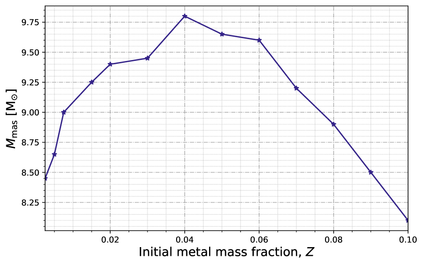
Figure 1: Initial mass to produce a Fe CCSNe, $M_{\rm mas}$, as a function of initial metallicity. These models were calculated with MESA version r23.05.1 and classified as massive if they have ONe cores greater than 1.37$M_{\odot}$ (Nomoto, 1984). They have canonical helium values calculated with the $\frac{\Delta Y}{\Delta Z}$ law. We model convection with the MLT, where $\alpha_{\rm MLT}=1.931$ (calibrated in Cinquegrana & Joyce 2022) and use OPAL opacities for high temperature regions, custom ÆSOPUS tables for low temperature regions. We model mass on the red giant branch using Reimers (1975) and Blöcker (1995) for mass loss along the asymptotic giant branch (AGB). We use the Ledoux criteria for convective stability, allowing us to include semiconvection and thermohaline mixing. Finally, we use the predictive mixing algorithm to find the borders between convective and radiative regions, and include convective overshooting using the prescription of Herwig (2000).

Table 2: $M_{\rm mas}$ values in [$M_{\odot}$] as a function of initial metal mass fraction, $Z$.

$Z\rightarrow$

0.0025

0.005

0.0075

0.014

0.02

0.03

0.04

0.05

0.06

0.07

0.08

0.09

0.10

References

to

$\downarrow$

0.015

This work

8.45

8.65

9.0

9.25

9.4

9.5

9.8

9.65

9.6

9.2

8.9

8.5

8.1

Eldridge & Tout (2004), no OS

–

–

–

–

9.5

10

10

10

–

–

–

–

–

with OS

–

–

–

–

7

7.5

7.5

7.5

–

–

–

–

–

Siess (2007b), no OS

–

–

–

–

10.93

–

10.89

–

–

–

–

–

–

with OS

–

–

–

–

8.83

–

–

–

–

–

–

–

–

Poelarends et al. (2008), STERN

–

–

–

–

13

–

–

–

–

–

–

–

–

EVOL

–

–

–

–

10.5

–

–

–

–

–

–

–

–

KEPLER

–

–

–

–

9.2

–

–

–

–

–

–

–

–

Ibeling & Heger (2013)

8.65

8.95

9.05

9.35

9.5

9.6

9.85

–

–

–

–

–

–

Jones et al. (2013)

–

–

–

9.5

–

–

–

–

–

–

–

–

–

Doherty et al. (2015)

–

–

–

–

9.9

–

–

–

–

–

–

–

–

Woosley & Heger (2015)

–

–

–

9

–

–

–

–

–

–

–

–

–

Table 3: Relevant input physics for the models shown in Figure. 4. Here, CT = treatment of convection, CS = convective stability criterion, CBA = convective boundary placement algorithm, SC = semiconvection, NG = data not provided.

Reference	Symbol	Code	Zmax	CT	CS	CBA	SC
This work		MESA	0.10	MLT	Ledoux	Herwig (2000)	Yes
				$\alpha_{\rm MLT}$=1.931
Eldridge & Tout (2004)		STARS	0.05	MLT	(Modified) schwarzschild⋆	Schröder et al. (1997)	Yes
				$\alpha_{\rm MLT}$=2.0
—		—	—	—	—	No	—
Siess (2007b)		STAREVOL	0.04	MLT	Schwarzschild	No	No
				$\alpha_{\rm MLT}$=1.75
—		—	—	—	—	Freytag et al. (1996)	—
						Blöcker et al. (1998)
Poelarends et al. (2008)		STERN	0.02	MLT	Ledoux	NG	Yes
—		EVOL	0.02	MLT	Schwarzschild	Herwig (2000)	No
—		KEPLER	0.02	MLT	Ledoux	Yes	Yes
Ibeling & Heger (2013)		MESA	0.04	MLT	NG	Freytag et al. (1996)	NG
						Herwig (2000)
Jones et al. (2013)		MESA	0.014	MLT	Schwarzschild†	Freytag et al. (1996)	No
				$\alpha_{\rm MLT}$=1.73		Herwig (2000)
Doherty et al. (2015)		MONSTAR	0.02	MLT	Ledoux	Lattanzio (1986)	NG
				$\alpha_{\rm MLT}$=1.75
Woosley & Heger (2015)		KEPLER	0.015	MLT	Ledoux	Yes	Yes

$\star$ Eldridge & Tout (2004) use a modified version of the Schwarschild criterion with an extra term that allows for the modelling of semi-convection and diffusive overshooting. See §  2.1.2 of Eldridge & Tout (2004) and Schröder et al. (1997).
$\dagger$ Jones et al. (2013) use the Schwarschild criterion for the majority of their evolution, but switch to Ledoux during late stage evolution for some models.

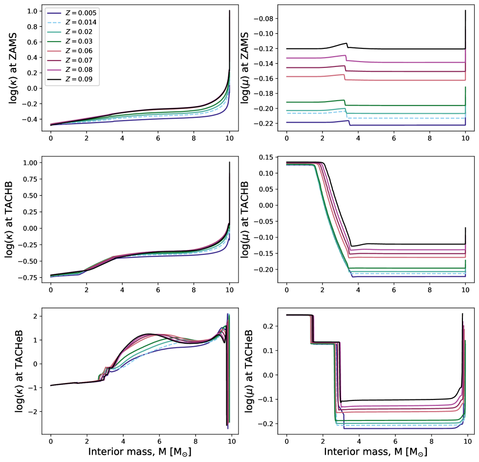
Figure 2: The $\kappa$ and $\mu$ profiles of a set of 10$M_{\odot}$ models. We vary $Z$ between $Z=0.005$ and $Z=0.09$. Snapshots are provided at the zero-age main sequence, terminal age core H burning and terminal age core He burning (when ¹H and ⁴He drop below $1\times 10^{-3}$).

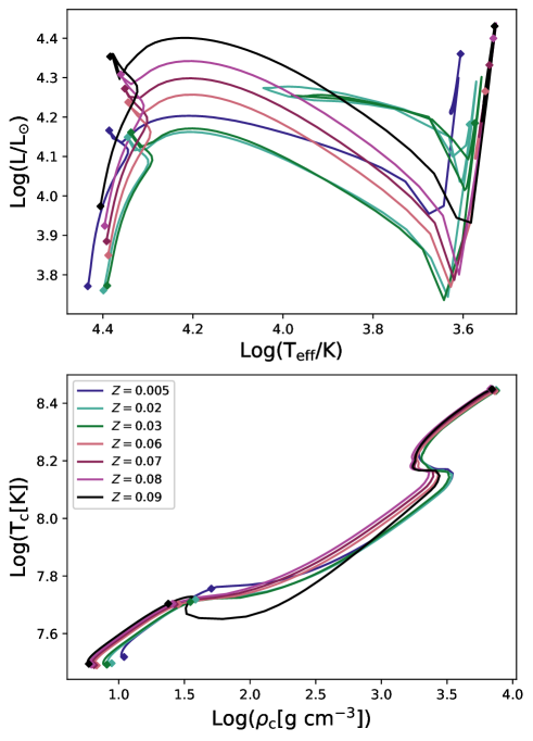
Figure 3: The stellar tracks (upper panel) of 10$M_{\odot}$ models, $Z$ between $Z=0.005$ and $Z=0.09$, and their $T_{c}$ and $\rho_{c}$ behaviour (lower panel).

Our primary results are presented in Figure. 1 and Table. 2. We find higher initial masses are required for models to undergo Fe CCSNe as the initial metallicity increases from $Z\approx 1\times 10^{-3}$ to $\approx 2$$Z_{\odot}$. That is, the magnitude of the H exhausted core mass for models in this range decreases with increasing $Z$. For $Z>0.05$ (which also corresponds to the maximum metallicity currently tested in the literature), these trends reverse. With increasing metallicity, the H exhausted core mass now begins to increase again, so lower initial masses will undergo Fe CCSNe as metallicity increases to $Z=0.10$.

It is important to understand why this trend reversal occurs at the highest metallicities we consider. As the initial metal content in a gas increases, so too do the opacity ($\kappa$) and the mean molecular weight ($\mu$) of the gas. If we consider the mass luminosity relation,

$$L\propto\frac{\mu^{4}M^{3}}{\kappa},$$ (2)

and the Stefan-Boltzmann relationship,

$$L=4\pi R^{2}\sigma T_{\rm eff}^{4},$$ (3)

we can see that an increasing $\kappa$ leads to lower luminosities and effective temperatures. Yet, an increasing $\mu$ leads to higher luminosities and effective temperatures. Although Equations 2 and 3 are simplifications of the treatments in MESA and other stellar evolution codes, the balance between $\kappa$ and chemical composition remains relevant, and we see these opposing effects of $\kappa$ vs $\mu$ dominate for different metallicity ranges.

The impact of the higher $\kappa$ and $\mu$ in our metal-rich models manifests in a variety of stellar processes. For the following discussion, we consider the metal-rich range to extend from $Z=0.014$ (roughly solar metallicity) to $Z=0.10$ (10% metals). In Figure 2, we show the $\kappa$ and $\mu$ profiles of a set of 10$M_{\odot}$ models, we vary $Z$ between $Z=0.005$ and $Z=0.09$. Snapshots are provided at the ZAMS, terminal age core H burning (TACHB) and TACHeB.

At the ZAMS, $\kappa$ and $\mu$ in the stellar envelope increases with initial metallicity. The opacity reaches a plateau in the higher metallicity range, with the $Z=0.06,0.07,0.08$ and $Z=0.09$ models achieving the same values. At the end of core H burning, the variation in $\kappa$ (between the models) in the envelope has decreased, but there still remains a significant difference between the $\mu$ curves in the stellar envelopes of the different models. It appears that an increasing gas metal content primarily impacts the envelopes of these models. The feature in the $\kappa$ plot at the TACHeB is the Fe $\kappa$ bump, identified in the early 1990s (Rogers & Iglesias, 1992; Seaton, 1995), which occurs at $\log T\approx 5.3$K.

In Figure. 3, we show the stellar tracks of these same models as well as their central temperatures ($T_{c}$) and densities ($\rho_{c}$). The $Z=0.005,0.02$ and $0.03$ models evolve onto ZAMS with roughly the same luminosity, but the $Z=0.02,0.03$ cases emerge with lower effective temperatures. These two models maintain lower $L$ and $T_{\rm eff}$, in comparison to the $Z=0.005$ model, for their evolution up to TACHeB. They begin their ascent of the red giant branch at lower $L$ ($\Delta L\approx 0.25$$L_{\odot}$) and experience much longer blue loops (see Walmswell et al. 2015) than any of the other models. These loops are very sensitive to microphysics choices (e.g. the ¹⁴N($p,\gamma)^{15}$O rate, see Weiss et al. 2005). Consequently, there remains a lack of consensus in the literature with respect to how the loops should behave as their initial metal content is varied. The models with $Z\geq 0.06$ initiate (and complete) core H burning (and He burning) at $L$ values that increase with $Z$. In terms of their central conditions, all the metal-rich models show slightly cooler temperatures and lower densities than the $Z=0.005$ case at ZAMS and TACHB but evolve through the phases with slightly warmer tracks. All models complete core He burning at approximately the same temperature and density.

To summarize, as metallicity increases, both the opacity and mean molecular weight of the gas also increase. The difference in $\kappa$ and $\mu$ between the $Z=0.005$ case and the metal-rich models is most significant in the stellar envelope. At the lower end of the metal-rich range ($Z=0.02,0.03$), the models experience cooler and slightly less luminous core H and He burning phases, which leads to H exhausted core masses that decrease in magnitude with $Z$. Consequently, these models require higher initial masses for key burning phases, to make up for their less massive cores. The models at the higher end of the metal-rich range ($Z\geq 0.06$) experience more luminous and warmer main sequence burning lifetimes, but still have cooler and less luminous surfaces as they ascend the giant branches. The conflicting behaviour of these metal-rich models is driven by the competition between the effects of the higher $\kappa$ and $\mu$. The most enriched $Z$ models possess greater initial He levels, represented by the $\frac{\Delta Y}{\Delta Z}$ law (see Equation. 1). Higher $Y_{i}$ further drives up $\mu$, and the associated properties with a higher $\mu$. Namely, the higher $T_{\rm eff}$ and $L$ lead to more efficient core burning phases and thus more massive H exhausted cores. Consequently, these models require lower initial masses for higher order burning stages with increasing $Z$ (e.g. core C ignition).

Low and intermediate mass metal-rich models experience mass loss rates that increase with $Z$. Karakas et al. (2022) and Cinquegrana & Karakas (2022), found the same models show drastically reduced mixing efficiencies for third dredge up (TDU) episodes on the thermally pulsing AGB (TP-AGB). Although low mass models will still endure the first dredge up – and intermediate models the second dredge up as well — the first two dredge up events only mix H burning products up to the stellar surface. The TDU is the first opportunity for these models to mix He burning products and potentially elements produced by the slow neutron capture process (s-process) up to the surface. Thus, eventually those products can be contributed back to the interstellar medium as the envelope is eroded by stellar winds, rather than remaining locked inside the white dwarf remnant. Due to their lower effective temperatures, very metal-rich models are also often unable to ignite H at the base of their convective envelopes on the TP-AGB, known as hot bottom burning. The higher mass loss rates of the models shortens their AGB lifetimes and thus they have less opportunities to experience their less efficient TDU and hot bottom burning episodes. Interestingly, we found that the second dredge up episode (for intermediate mass stars, on the early red giant branch) is largely metallicity independent (see Karakas et al. 2022). Thus even though the net yields of these models are depleted in He burning and s-process products, they are rich in secondary H burning nucleosynthesis products.

We end this discussion by emphasizing that all the downstream implications of a high $Z$ (e.g. faster mass loss rates, lower TDU efficiencies) increase monotonically with $Z$, regardless of the competition between $\kappa$ and $\mu$. The core mass, however, does not.

Lastly, it is worth noting that the reversal in trend we see for $M_{\text{mas}}$ is sensitive to the scaling of the initial He abundance with the initial $Z$ abundance. Whether He does scale linearly with metallicity (and by the same rate in all regions of the universe) is unknown, as is the exact value of the primordial He abundance, $Y_{0}$. Perhaps most uncertain is the value of $\frac{\Delta Y}{\Delta Z}$. In this work, we use $\frac{\Delta Y}{\Delta Z}=2.1$ (Casagrande et al., 2007a), but this quantity is very difficult to constrain. To do so, we need to measure the stellar He abundance directly, which is only feasible in stars with $\rm T_{eff}>8000$K (i.e. main sequence stars with initial masses greater than 1.5$M_{\odot}$; Valcarce et al. 2013b). A range of methods to estimate $\frac{\Delta Y}{\Delta Z}$, both observational and theoretical, yield values of $\frac{\Delta Y}{\Delta Z}$ between 0.7 to 10 (e.g. Faulkner, 1967; Perrin et al., 1977; Renzini, 1994; Fernandes et al., 1996; Pagel & Portinari, 1998; Ribas et al., 2000; Chiappini et al., 2002; Jimenez et al., 2003; Salaris et al., 2004; Balser, 2006; Izotov et al., 2007; Casagrande et al., 2007b; Gennaro et al., 2010; Portinari et al., 2010; Brogaard et al., 2012; Martig et al., 2015; Joyce & Chaboyer, 2018b). This uncertainty aside, the precise value of $\frac{\Delta Y}{\Delta Z}$ will have no effect on the qualitative trend. The only way this could have an impact would be if this value were not the same universally.

4 Literature comparison

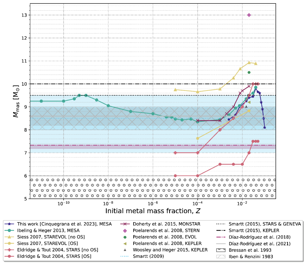
Figure 4: A comparison of our calculated $M_{\rm mas}$ against that currently available in the literature, where $M_{\rm mas}$ is the minimum initial mass required for a star to undergo an Fe CCSNe. A copy of this figure using a linear scale, without shading is included in the appendix, 8. The relevant input physics used in each set of models, where available, is listed in Table. 3. Isolated curves are theoretically derived $M_{\rm mas}$ values. The hatched regions (corresponding to Iben & Renzini 1983 and Bressan et al. 1993 are metallicity independent approximations for $M_{\rm mas}$, often used in galactic chemical evolution simulations. Smartt (2009), Díaz-Rodríguez et al. (2018) and Díaz-Rodríguez et al. (2021) are $M_{\rm mas}$ values derived using observational quantities. The upper and lower uncertainties for these measured quantities are indicated by the shaded regions in the same colour.

In Figure 4, we compare our results to the theoretically derived results of Eldridge & Tout (2004), Siess (2007b), Poelarends et al. (2008), Ibeling & Heger (2013), Jones et al. (2013), Doherty et al. (2015) and Woosley & Heger (2015). We also highlight the mass regions that are commonly used in galactic chemical evolution simulations (Iben & Renzini 1983; Bressan et al. 1993 are theoretically derived; Smartt 2009 is derived using observational quantities). A version of this figure using a linear scale and without shading is included in the appendix, 8. Our values match those of Ibeling & Heger (2013) very well across the entire metallicity range. There is a maximum variation of 3.4% between our $M_{\rm mas}$ values; on average they differ by $\sim 1.4$%. This difference extends to 1-5.2% between our results and those of Eldridge & Tout (2004) models with no overshoot, Woosley & Heger (2015), Jones et al. (2013), Doherty et al. (2015) and the Poelarends et al. (2008) KEPLER models. There is a 6.3% deviation between ours and Siess (2007b) with overshoot. The Siess (2007b) models with no overshoot and the EVOL models from Poelarends et al. (2008) calculate significantly higher values for $M_{\rm mas}$. There is a 10-15% difference between those models and ours. Eldridge & Tout (2004) models with overshoot and the Poelarends et al. (2008) STERN model show the largest variation, approximately 23-32% between those and our values for $M_{\rm mas}$. Regardless of the quantitative difference in values between the models, we note that the overall shapes of the $M_{\rm mas}-Z$ curves are very similar.

We also compare our models and calculations in the literature against the shaded regions, representing common non-metallicity-dependent approximations for $M_{\rm mas}$ used in galactic chemical evolution simulations. The Iben & Renzini (1983) range ($8-9$$M_{\odot}$) encompasses the majority of the curves for $1\times 10^{-3}<Z<0.01$. It also contains our highest metallicity models, $Z=0.09$ and $0.10$. The Smartt (2009) range is larger, 8$\pm$1$M_{\odot}$, and also contains the Eldridge & Tout (2004) models with no overshoot for $1\times 10^{-5}<Z<1\times 10^{-3}$. The Bressan et al. (1993) range ($5-6$$M_{\odot}$) misses all but the Eldridge & Tout (2004) overshoot values for $Z=1\times 10^{-4}$ and $1\times 10^{-5}$. All three completely miss the metallicity range between $Z=1\times 10^{-2.5}$ and $Z=0.08$, which is particularly important for simulations of spiral galaxies with solar (or super solar) metallicity bulges. Given a typical IMF, such as (Salpeter, 1955), favour low-mass stars, the consequences of using one of these non-metallicity-dependent ranges is the over prediction of SNe events at solar metallicity and miscalculation of appropriate yields. Likewise, if one uses a metallicity-dependent curve, e.g. the Ibeling & Heger (2013) values, and extrapolates for $Z>0.04$, then one is likely under-predicting the number of SNe occurring in the most metal-rich regions.

5 Key modeling uncertainties

In Table 3, we summarize the various physics prescriptions adopted by each set of authors whose results are shown in Figure 4. The physical components described include convective treatment, convective boundary placement algorithms, semiconvection treatment, as well as the evolution code used. We discuss the most critical physical choices and their respective contributions to the uncertainty of $M_{\rm mas}$. We focus on our current understanding of these processes and comment on the validity of their implementation in stellar evolution codes. There are, of course, many other uncertainties related to stellar modelling that we will not discuss here (c.f. Choi et al. 2018; Tayar et al. 2022; Joyce et al. 2023); we have chosen in this study to focus on the assumptions that are most pertinent to our derivation of $M_{\rm mas}$.

5.1 Convective boundaries

The border that divides convective and radiative regions in a stellar interior can be found using the Schwarzschild criterion for dynamic stability,

$$\nabla_{\rm rad}<\nabla_{\rm ad}.$$ (4)

$\nabla_{\rm rad}$ and $\nabla_{\rm ad}$ represent the radiative and adiabatic temperature gradients. The general temperature gradient, $\nabla$, is defined as:

$$\nabla=\frac{d\ln T}{d\ln P}=\frac{P}{T}\frac{dT}{dP}.$$ (5)

One may also use the Ledoux criterion, which reduces to Schwarzschild where there is no composition gradient:

$$\nabla_{\rm rad}<\nabla_{\rm ad}+\frac{\phi}{\delta}\nabla_{\mu}.$$ (6)

Here, $\phi$ ($\delta$) represents the density gradient with respect to composition (temperature) and $\nabla_{\mu}$ is the composition gradient. Given that $\nabla_{\rm rad}<\nabla_{\rm ad}$ denotes a region in dynamic stability, $\nabla_{\rm rad}=\nabla_{\rm ad}$ indicates the location at which the convective acceleration reduces to zero. With a proper implementation of the Ledoux and Schwarzschild criteria, both Equations. 4 and 6 should identify the same border location (Gabriel et al., 2014). Anders et al. (2022) demonstrate this by considering how convective zones interact with Ledoux–stable regions in 3D hydrodynamical simulations. They find that where the evolution timescale is significantly greater than the convective mixing timescale, the convective borders defined by both criteria are equivalent.

A common approach to locate the convective–radiative boundary in stellar structure calculations is to use a sign-change algorithm, as discussed in Gabriel et al. (2014); Paxton et al. (2018) and Paxton et al. (2019). Let the discriminant $y$ for the Schwarzschild and Ledoux criteria be given by

$$y_{s}\equiv\nabla_{\rm rad}-\nabla_{\rm ad},$$ (7)

and

$$y_{l}\equiv\nabla_{\rm rad}-(\nabla_{\rm ad}+\frac{\phi}{\delta}\nabla_{\mu}),$$ (8)

respectively. If we were to scan along the radius of a stellar model, the sign of the applicable dynamical stability criterion (either Equation 4 or 6) would reverse at the transition from a convective to radiative region. At this point, the relevant discriminant should reduce to zero on both sides of the border. In practice, this radial search is performed first from the convective side of the border, given that the location at which convective acceleration reduces to zero is only meaningful in a convective region.

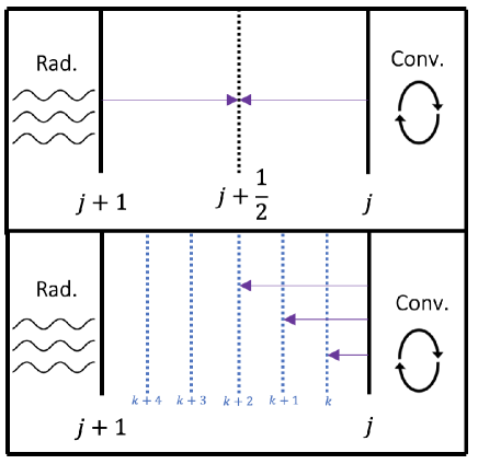
Figure 5: Depiction of the sign-change algorithm (upper panel) and the subgrid physics model (or “direct search” algorithm; lower panel) used in 1D stellar evolution codes to locate the boundaries between convective and radiative regions. $j$ and $j+1$ are the mesh shells which represent the points at which the discriminants ($y_{s}$ and $y_{l}$, see Equations. 7 and 8) first reduce to zero on the radiative and convective sides of the boundary, respectively. $k$ to $k+5$ represent a finer resolution of the region between $j$ and $j+1$.

We paint a simplified picture of the sign-change algorithm in the upper panel of Figure 5. Here, we have located the mesh shells, $j$ and $j+1$. These represent the points at which the discriminant first reduces to zero on the radiative and convective sides of the boundary, respectively. Mesh shell $j$ indicates the location at which the acceleration of the convective eddies reduces to zero, but they will still have some non-zero velocity. Consequently, these eddies may potentially overshoot some distance beyond $\nabla_{\rm rad}=\nabla_{\rm ad}$. So, the actual convective border ($v=0$) is commonly adjusted ad hoc by interpolating between the two mass shells $j$ and $j+1$. As described in Gabriel et al. (2014), this approach is sufficient while using the Schwarzschild criterion with a continuous composition gradient across the convective border (Gabriel et al., 2014). This occurs, for example, on the zero-age main sequence and at the red giant branch bump (due to thermohaline mixing). However, an issue arises once a composition discontinuity forms, given the difficulty of smoothing over such discrepancies numerically. In this case, $\nabla_{\rm rad}=\nabla_{\rm ad}$ is only met on the convective side of the border. On the radiative side, we hold the inequality $\nabla_{\rm rad}<\nabla_{\rm ad}$. In the context of a convective core, using the sign-change algorithm with Schwarzschild and a composition discontinuity (or Ledoux with and without a discontinuity) results in the incorrect placement of the border. This typically inhibits the growth of the convective zone and so results in a less massive core.

A more precise way to locate the convective border, whilst dealing with composition discontinuities, is to use a subgrid physics model. We define this approach as a “direct search algorithm,” depicted in the lower panel of Figure 5. Direct search algorithms begin with a candidate boundary, $j$. We then iteratively improve the resolution between $j$ and $j+1$ and consider how the discriminant would change if some intermediate, finer mesh shell, $k$, located between $j$ and $j+1$, were part of the convective region. If $k$ is unstable to convection under the relevant stability criterion, it is allocated to the well-mixed convective region. The process is repeated for mesh point $k+1$; if $k+1$ is still stable under these convective conditions, then $k$ is considered the formal boundary. Examples of direct search algorithms in use are the relaxation method (or search for convective neutrality) defined in Lattanzio (1986) and implemented in the Monash code (and MONSTAR), as well as the “predictive mixing” and “convective premixing” schemes implemented in MESA (see Paxton et al. 2018 and Paxton et al. 2019, respectively, for thorough discussions of these). Compared to the sign-change algorithm, direct search tends to result in larger convective zones. We see this in the more efficient TDU mixing episodes on the TP-AGB when using the relaxation direct search algorithm, as the convective envelope is able to penetrate further into the internal radiative region (i.e. Frost & Lattanzio 1996).

Finally, a third type of boundary search algorithm exists, commonly known as convective overshoot (Shaviv & Salpeter, 1973) or convective boundary mixing (Herwig, 2000). In the case of overshoot, we make manual adjustments to shift the border beyond mesh shell $j$. We define a particular distance, in units of pressure scale height ($\rm H_{p}$), over which material can permeate beyond the formal boundary, $j$. There are examples of overshoot algorithms in the literature using both diffusive and instantaneous treatments. The former include Freytag et al. (1996); Schröder et al. (1997); Bressan et al. (1981); Herwig (2000), the latter Karakas (2010); Kamath et al. (2012). In comparison to sign-change and direct search, overshoot often leads to the largest growth of the convective core.

We know of several observed abundance anomalies that cannot be reproduced with standard stellar models (i.e. those that assume convection is the only form of mixing). For example, standard models incorrectly predict changes in the abundances of light elements–carbon, lithium and nitrogen–following the first dredge up event on the red giant branch (Carbon et al., 1982; Pilachowski, 1986; Gilroy, 1989; Kraft, 1994; Charbonnel, 1994; Charbonnel & do Nascimento Jr, 1998; Gratton et al., 2000; Shetrone et al., 2019; Tayar & Joyce, 2022). As noted in Schröder et al. (1997), “…the Achilles’ heel of modern evolutionary codes is (still) the very simple representation of convection.” This is very much still relevant, some 25 years later. Not only is mixing in stellar interiors an extremely uncertain process, but we are also trying to approximate a 3D process in 1D. Some of the abundance discrepancies between theory and observation can be forced into consistency using a considerable amount of convective overshooting (e.g. Joyce & Chaboyer 2015). However, this amount of overshooting is applied ad hoc, meaning it is not necessarily physical. More likely, it is a consequence of our current assumption that convection is the only mechanism responsible for mixing in stellar interiors. There have been other mechanisms hypothesized in the literature including rotation–induced mixing (Palacios et al., 2003), atomic diffusion (Bahcall et al., 1995; Henney & Ulrich, 1995; Gabriel, 1997; Castellani et al., 1997; Chaboyer et al., 2001; Bertelli Motta et al., 2018; Liu et al., 2019; Semenova et al., 2020), internal gravity waves (Garcia Lopez & Spruit, 1991; Denissenkov & Tout, 2003; Rogers et al., 2013; Varghese et al., 2022) and thermohaline mixing (Charbonnel & Zahn, 2007; Charbonnel & Lagarde, 2010; Lagarde et al., 2011, 2012; Lattanzio et al., 2015; Angelou et al., 2015; Henkel et al., 2017; Fraser et al., 2022). The benefit, then, to overshoot is that it can be manipulated to absorb other 3D effects that are not included in our 1D models. For example, Schröder et al. (1997) use overshoot to replicate giant star luminosities in $\zeta$ Aurigae systems. Kamath et al. (2012) require a significant amount of overshoot (3$\rm H_{p}$, on top of the relaxation algorithm) for their models to match observed C and O abundances in Magellanic Cloud clusters.

We note that a powerful constraint for the mixing profiles in stars arises from asteroseismology by using acoustic (p) and gravity (g) modes as probes. For example, Pedersen et al. (2021) utilize the g mode to constrain the mixing profile of stars, given that g modes are quite sensitive to the core-boundary layer. They calculate mixing profiles for 26 stars with initial masses between 3 and 10$M_{\odot}$, based on observed g mode period spacing patterns, and compare these profiles against a grid of theoretically derived mixing profiles. These theoretical profiles contain a variety of the common mixing assumptions used in the literature. They find that $\approx 65$% of the sample profiles are better modelled using an instantaneous approximation for overshoot, as opposed to diffusive, at the core boundary layer. This method of course contains its own uncertainties and approximations, and we are still comparing 1D phenomenological prescriptions against asteroseismic oscillations from 3D stars. However, this method is one of few with which we can infer what goes in underneath the stellar surface and the initial results are promising.

With our current understanding, it perhaps makes the most sense to consider models utilizing sign-change algorithms as conservative estimates of $M_{\rm mas}$, those using convective overshooting as upper limits of $M_{\rm mas}$, and those using direct search algorithms somewhere in the middle. With this in mind, the appearance of overshooting in models of Figure 4 does not predict whether $M_{\rm mas}$ falls within a particular mass range, just that it results in a larger core mass and thus lower $M_{\rm mas}$. In both the Siess (2007b) and Eldridge & Tout (2004) models, the inclusion of overshoot lowers the $M_{\rm mas}$ quantity by $\approx 1-1.5$$M_{\odot}$. However, for Siess (2007b) (using STAREVOL), this transition is from $M_{\rm mas}=10.93$$M_{\odot}$ (no core overshoot) to 8.83$M_{\odot}$ (with core overshoot) at $Z=0.02$. For Eldridge & Tout (2004) (using STARS), the transition is from $M_{\rm mas}=9.5$$M_{\odot}$ (no core overshoot) to 7$M_{\odot}$ (with core overshoot) at $Z=0.02$. Both codes decrease $M_{\rm mas}$ by $>$2$M_{\odot}$, but Siess (2007b) is shifted “into” the common range with overshoot, whereas Eldridge & Tout (2004) is shifted “out.” Although the algorithms that we use to define convective borders contribute a large uncertainty, there is clearly more at play here with $M_{\rm mas}$. Both Siess (2007b) and Eldridge & Tout (2004) use different overshoot prescriptions (Freytag et al. 1996; Herwig 2000 for the former, Schröder et al. 1997 for the latter), but it is unlikely that this makes a significant difference given that the inclusion of either prescription lowers the core masses by a similar magnitude (30% and 21%). This suggests that there is either a combination of other physical parameters that accumulate to make a significant difference and/or that the numerics of the software instruments themselves have a more substantial dependence on the core mass beyond the treatment of convective boundaries. In the next few subsections, we discuss other approximations that will likely make lesser, but non-negligible, contributions to variations in $M_{\rm mas}$ between evolution codes. We do not discuss here the impact software architecture can enact on evolution results (even when implementing the same input physics) given that this was the focus of Paper 1 (Cinquegrana et al., 2022). On this topic, we refer the interested reader to the following works focused on the inter-comparison of particular stellar evolution tools:

• Paxton et al. (2010), compares MESA against BaSTI (a Bag of Stellar Tracks and Isochrones; Pietrinferni et al. 2004; Hidalgo et al. 2018; Pietrinferni et al. 2021; Salaris et al. 2022), FRANEC (the Frascati Raphson Newton Evolutionary Code; Chieffi et al. 1998; Limongi & Chieffi 2006), DSEP (the Dartmouth Stellar Evolution Program; Dotter et al. 2007), GARSTEC (the Garching Stellar Evolution Code; Weiss & Schlattl 2008) and EVOL.

• Martins & Palacios (2013), compares MESA and STAREVOL against the Geneva stellar evolution code (Eggenberger et al. 2008), STERN, PARSEC and FRANEC.

• Sukhbold & Woosley (2014), compares MESA and KEPLER.

• Jones et al. (2015), compares GENEC, KEPLER and MESA.

• Joyce & Chaboyer (2015) compares DSEP against BaSTI, YREC, PARSEC, and others.

• Aguirre et al. (2020), compares nine stellar evolution codes: BaSTI, GARSTEC, MESA, MONSTAR, YREC (the Yale Rotating Stellar Evolution Code; Demarque et al. 2008), ASTEC (the Aarhus STellar Evolution Code; Christensen-Dalsgaard 2008), CESTAM (Code d’Evolution Stellaire Adaptatif et Modulaire; Morel & Lebreton 2008; Marques et al. 2013; Deal et al. 2018), LPCODE (La Plata Observatory, Althaus et al. 2003) and YaPSI (Skumanich 1972).

• Agrawal et al. (2022) compares Geneva, MESA, PARSEC, BPASS (Binary Population and Spectral Synthesis; Eldridge et al. 2017), BoOST (Bonn Optimized Stellar Tracks; Szécsi et al. 2022).

• Campilho et al. (2022) compares MESA against the Montreal/Montpellier stellar evolution code (Turcotte et al. 1998; Richer et al. 2000) and with CESTAM.

• Paper I Cinquegrana et al. (2022), compares MESA against the Monash stellar evolution code.

5.2 Treatment of convection

Convection is an extremely uncertain process to model in 1D. Whilst we were previously concerned with the borders that define convective regions, here we focus on the actual convective treatment. To model a star, we need to solve the equations of stellar structure and calculate the general temperature gradient, $\nabla$ (defined previoulsy in Equation. 5). In regions of dynamic stability, energy is transported via radiation. Thus, $\nabla$ comprises radiative flux contributions:

$$F_{\rm rad}=\frac{4acG}{3}\frac{T^{4}m}{\kappa Pr^{2}}\nabla,$$ (9)

where $a$ is the radiation density constant and $c,G,T,m,P,r$ have their usual meanings. In regions of dynamic instability, some to all of the energy flux is transported via convection. In the superadiabatic case, the general temperature gradient, $\nabla$, comprises both radiative and convective flux contributions. The latter requires some approximation to compute in 1D; all works compared here utilize the Mixing Length Theory (MLT) of convection to do so (though some other stellar evolution codes do include alternatives, e.g. the Full Spectrum Turbulence model of Canuto & Mazzitelli 1991; Canuto et al. 1996, we do not examine results from these here). The MLT assumes that a mass "blob" will travel some distance, $\lambda$, before dissolving into its surroundings. Under this basic approximation, we can derive the following expression for $F_{\rm conv}$,

$$F_{\rm conv}=\frac{1}{2}\rho vc_{p}T\frac{\lambda}{\rm H_{p}}(\nabla-\nabla_{\rm ad}),$$ (10)

where $\rho$, $v$ and $T$ have their usual meanings, $c_{p}$ is the specific heat, $\nabla$ and $\nabla_{\rm ad}$ are the general (or true) and adiabatic temperature gradients. $\lambda$ is the mean free path of the gas element, $\rm H_{p}$ is the pressure scale height, and so $\frac{\lambda}{\rm H_{p}}$ is the mixing length parameter, $\alpha_{\rm MLT}$. Using this definition, we can approximate the true temperature gradient $\nabla$ in a given dynamically unstable region. For clarity, we also define the convective efficiency, $\Gamma$, which from Kippenhahn et al. (2012) is given by:

$$\Gamma=\frac{4}{3}\frac{F_{\rm conv}A}{\lambda}.$$ (11)

Here, $A$ is the cross section of the mass "blob" and $\lambda$ is the total energy loss. Given that the MLT is a phenomenological–rather than physical—model, $\alpha_{\rm MLT}$ must be calibrated for each stellar evolution code and ideally, each set of input physics. This calibration is typically performed against the Sun (e.g. Cinquegrana & Joyce 2022), although arguments have been made that the Sun is not always the best choice (Joyce & Chaboyer, 2018a, b). The MLT was originally established by Prandtl (1925) but first developed for stellar interiors by Böhm-Vitense (1958). Since then, it has been modified for specialization in optically thin (Henyey et al., 1965) and optically thick (Cox & Giuli, 1968) regimes. It is important to note, however, that the MLT only needs to be solved in regions of significant (but not too significant) super adiabaticity. Here, $\Gamma$ (from Equation. 11) is low and the true temperature gradient lies between $\nabla_{\rm rad}$ and $\nabla_{\rm ad}$. This occurs in the outer layers of giant star envelopes, where the temperature gradient must increase significantly to transport heat through the extremely opaque material. Convection in the central regions of stars is technically superadiabatic, but it is so efficient ($\Gamma\rightarrow\infty$) that we approximate $\nabla=\nabla_{\rm ad}$. Thus, there is no need to solve the MLT equations. On the other hand, if the region is too superadiabatic (e.g. the stellar photosphere, where $\Gamma\rightarrow 0$), then convective transport is so inefficient that radiation is carrying almost all the flux. In that case, we can approximate $\nabla=\nabla_{\rm rad}$ (see Joyce & Tayar 2023 for thorough coverage of this topic).

Although the MLT is not used to model core convection, the use of various MLT formulations (e.g. Böhm-Vitense 1958; Henyey et al. 1965; Cox & Giuli 1968; Bohm & Cassinelli 1971; Mihalas et al. 1978; Mihalas 1978; Kurucz 1979) and calibration methods for $\alpha_{\rm MLT}$ will have an indirect impact on the size of the core. Suppression of the surface convective flux—whether due to a small $\alpha_{\rm MLT}$, magnetism, certain atmospheric boundary conditions, or otherwise—leads to a corresponding structural re-alignment of the star that propagates to the inner-most point of the model. In essence, we are adjusting the boundary conditions of the coupled equations of stellar structure describing our model. The knock-on structural effects of small $\alpha_{\text{MLT}}$ is demonstrated in Joyce & Tayar (2023) for the case of a 1$M_{\odot}$, $Z_{\odot}$ model. On the main sequence, stars with initial masses between 0.5 and 1.2$M_{\odot}$ should have radiative cores with convective envelopes. However, in the case where $\alpha_{\rm MLT}$ is reduced below 0.5$\rm H_{p}$, the impediment to the expulsion of convective flux is so great that the 1$M_{\odot}$ model compensates by developing a convective core.

5.3 Semiconvection

At this point, we have discussed the fact that our treatment of convection and our placement of convective boundaries will have an impact on our H exhausted core (and thus, $M_{\rm mas}$). The aim of this section is to consider the effects of a more nuanced mixing process, semiconvection. Semiconvection, and its place within the context of stellar interiors, has been recognized by the astronomical community since the 1950s (Tayler, 1954; Schwarzschild & Härm, 1958). Since then, it is not the actual presence of these zones, but the extent of mixing that occurs inside of them, that has been hotly debated in the literature. In this section, we discuss our understanding of this process, what light it shines on semiconvective mixing efficiency, and lastly the potential impact this enacts on $M_{\rm mas}$.

Semiconvection is a type of double-diffusive instability, known as the oscillatory double-diffusive instability (ODDC), that occurs in regions that are thermally unstable (according to Eq. 4) but have a stable ($\mu<0$) composition gradient (according to Eq. 6):

$$\nabla_{\rm ad}<\nabla_{\rm rad}<\nabla_{\rm ad}+\frac{\phi}{\delta}\nabla_{\mu}.$$ (12)

Although stellar semiconvection has been discussed since the 1950s, it was not classified as ODDC until close to a decade later (Kato, 1966; Spiegel, 1969).

Our definition of semiconvection invites two main questions. Firstly, how do compositional gradients form in stars? The two most common examples of stable $\mu$ gradients are during core H burning in massive stars (example of a receding convective core) and during core He burning in low and intermediate mass stars (example of a growing convective core). The former situation, for example, arises from the fact that the opacity in main sequence massive stars is dominated by electron scattering, which is directly proportional to H content: $\kappa\sim(1+\rm X_{H})$. Thus, as the H content inside the convective core begins to decline, a higher percentage of the energy is now transported via radiation. Consequently, the boundary of the convective core begins to retreat. This leaves shells of H layers of increasing H content outwards, as each shell is successively less nuclearly processed than the previous. Secondly, we might then also ask what occurs once the conditions for semiconvection are met? The physics of double diffusive convection is fairly well understood, however earth-based experiments are often performed with high Prandtl number fluids (e.g. salt water, with $Pr\sim 7$) and so do not directly translate to stellar interiors, where Prandtl numbers and diffusivity ratios are much lower ($Pr$ and $\tau<<1$). The best chance we have at studying ODDC in this context is through 3D numerical simulations. For example, one of the most well-known studies is by Rosenblum et al. (2011), whose calculations extend down to $Pr=0.3$ and $\tau=0.3$. In their work, Rosenblum et al. (2011) identified the behaviour of two different types of ODDC that can arise in astrophysical conditions, homogeneous and layered, the latter of which occurs as the inverse density ratio,

$$\rm R^{-1}_{0}=\frac{\nabla_{\mu}}{\nabla-\nabla_{\rm ad}}$$ (13)

decreases below $\rm R^{-1}_{0}<1.35$. Layered convection, as the name suggests, forms in a series of many thin layers. These layers consist of both efficient, overturning convection and stagnant zones, stabilised by the density gradient, where transport occurs via molecular diffusion (which is much slower than convection). So, it is the stagnant zones that slow down the transport in these regions. For further discussion of the layering phenomenon, see Spruit (1992); Radko (2003); Spruit (2013); Zaussinger & Spruit (2013).

Moll et al. (2016) further showed that, given this layering results from the gamma instability (Radko, 2003), layered convection can further be split into two types, based on how the layers form. A crucial aspect to this discussion, however, is to consider how energy is transported through each type of semiconvective zone. Moll et al. (2016) confirm that the two different types of ODDC lead to very different energy transport efficiencies, with the fluxes in non-layered semiconvective zones no larger than those of conduction or molecular diffusion. Therefore, it is important to know what type of semiconvective zone we are modelling. Moore & Garaud (2016) find that semiconvective regions that are close to fully convective zones, such as in a convective core, are always layered.

We are most interested in the layered semiconvection which occurs adjacent to the fully convective core, that can potentially impact the convective core size. Layered convection is suspected to be significantly more efficient at transporting energy flux than the diffusive non-layered zones, however the extent of that efficiency is contested. Following the findings of Rosenblum et al. (2011), Moore & Garaud (2016) implemented the recent layered semiconvective approximation of Wood et al. (2013) into MESA. They find that the resultant mixing—which occurs in layered semiconvective zones—–is heavily dependent on the height of the layer. In fact, there is a critical layer height above which mixing is so efficient that it is comparable to using the Schwarzschild criterion and below which mixing is so inefficient that the model evolves the same as if they had used the Ledoux criterion. Importantly though, this critical layer height is appreciably smaller than the predicted minimum height for these layers. This implies that any layered convection occurring in stars is likely to have layer heights above this threshold and so the mixing is likely to be quite efficient. The results of Moore & Garaud (2016) therefore suggest that the magnitude of the convective core produced is comparable to that using the Schwarzschild criterion.

The current semiconvective prescriptions in use (of which there are many) reflect a variety of physical processes and approximations. The ideal implementation, that best reflects our current understanding, is one that can switch between using both non-layered and layered prescriptions for semiconvection based on the model. An example of this is provided by Mirouh et al. (2012); Wood et al. (2013); Moll et al. (2016). We lack information on the specific semiconvective prescriptions used in the papers to which we compare here, but we can get an approximate idea of the maximum potential difference between the models with the following: if the mixing in semiconvective regions is so efficient that the composition gradients are erased quickly and the region itself is absorbed into the convective core, then the maximum contribution semiconvection can add to the core mass is the difference between the core masses predicted by Ledoux and Schwarzschild criteria. If, by the other extreme, the mixing is completely inefficient, then the convective core will remain the magnitude predicted by the Ledoux criterion. So, the difference in the convective core magnitude between a model that uses the Ledoux criterion with no semiconvection prescription (no mixing), one that uses the Schwarzschild criterion (full convective mixing) and one that uses the Ledoux criterion with a semiconvective prescription (partial mixing) will be at most the difference in mass between the predictions of Schwarzschild vs Ledoux. The results of Moore & Garaud (2016) suggest that those using the Schwarzschild criterion will produce the largest (and hence most realistic) core masses.

With a proper implementation of ODDC semiconvection in their 3D simulations, Anders et al. (2022) find that the Ledoux and Schwarzschild criteria are equivalent on evolutionary timescales. The convection zone produced using the Ledoux criterion is initially smaller than the zone predicted by Schwarzschild, but the convection zone produced using the Ledoux criterion grows via entrainment, eventually to the same size as that predicted by the Schwarschild criterion. We note however, this was achieved by properly modelling ODDC semiconvection. For 1D simulations, they recommend using the Schwarzschild criterion.

To provide a quantitative description of the impact of these choices on convection zone size, in Figure 6 we show the progression of the convective core growth of 9.45$M_{\odot}$ models with $Z=0.02$ from the ZAMS to TACHeB when using the Ledoux or Schwarzschild stability criterion, and both with and without convective overshoot. For the models without convective overshooting (solid lines), there is an observable discrepancy between all the convective core masses on the main sequence, but this difference becomes most pronounced when the model undergoes core He burning. All models converge to approximately the same core mass at TACHeB ($\approx 0.7$$M_{\odot}$), except for the Ledoux model with the lowest semiconvective efficiency (as $\alpha_{\rm SC}\rightarrow 0$, the convective border reduces to that predicted by the Ledoux criteria alone). The convective core of this model is $\approx 0.4$$M_{\odot}$ at TACHeB, instead. The difference in the convective core masses with overshoot are much less significant (also found in Kaiser et al. 2020, to which we refer the reader for a detailed discussion into the variation of convective zone growth with different stability criteria and overshooting efficiencies).

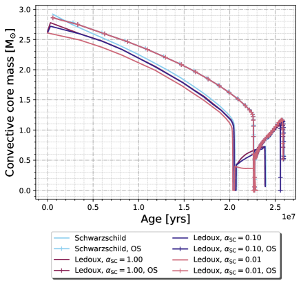
Figure 6: The progression of the convective core growth in 9.45$M_{\odot}$ models with $Z=0.02$ from the zero-age main sequence to the end of core He burning (TACHeB). The models use either the Schwarzschild or Ledoux stability criterion, with varying levels of semi convective efficiency and convective overshoot.

5.4 Carbon fusion reaction rates

Nuclear reaction rates, in general, comprise a major role in stellar modelling uncertainties (e.g. Lugaro et al., 2004; Karakas et al., 2006; Herwig et al., 2006; Izzard et al., 2007; Van Raai et al., 2008), particularly for later burning stages as found by Fields et al. (2018). However, the uncertainties of the C burning rate, ¹²C$+$¹²C, are particularly important for stellar structure. In fact, Fields et al. (2018) test the impact of 665 temperature-dependent reaction rate uncertainties (from the STARLIB library, Sallaska et al. 2013) on various stellar modeling quantities. At core C and Ne depletion, they deem the ¹²C(¹²C, p)²³Na rate the key reaction that governs the size of the ONe core mass, which makes this reaction pertinent to our discussion.

C burning occurs for central temperatures greater than $T_{c}>0.5\times 10^{8}$K, where ¹²C particles can fuse together to produce the compound nucleus, ²⁴Mg, which can then decay via three channels: ¹²C(¹²C, $\alpha$)²⁰Ne, ¹²C(¹²C, p)²³Na or ¹²C(¹²C, n)²³Mg. The astrophysical temperature range for quiescent C burning ($\approx$ 0.8 to 1.2$\times 10^{8}$K; Tumino et al. 2021) corresponds to energies of $\approx$ 1-3MeV. As a result, direct measurements of the ¹²C$+$¹²C reaction rates are extremely difficult to perform due to the increasingly small particle cross sections that accompany low energies (see Monpribat et al. 2022 for a thorough historical overview of the ¹²C$+$¹²C problem and experiments). In practice, then, C-fusion rates are generally measured at higher energies of $>2$MeV and extrapolated down to sub-coulomb energies. The major issue that arises with this method is the possible presence of unknown resonance (Spillane et al., 2007) or hindrance (Jiang et al., 2007) effects that are suggested to exist around the Gamow window, $\approx 1.5$MeV. The two phenomena have opposing consequences, with the former predicting our extrapolated rates are too slow and the latter, too fast.

Faster (slower) carbon burning rates result in lower (higher) core carbon ignition temperatures (Pignatari et al., 2012; Bennett et al., 2012; Chen et al., 2014; Fields et al., 2018). For example, Monpribat et al. (2022) present two new sets of ¹²C$+$¹²C rates—one based on the hindrance model, the other including a resonance contribution—and compare how these new rates impact the evolution of 12$M_{\odot}$ and 25$M_{\odot}$ models as compared to the standard Caughlan & Fowler (1988) ¹²C$+$¹²C rate. They find that the models using the hindrance model (and thus a lower rate) ignite carbon at a core temperature 10% greater than in the models using the faster rates. Higher carbon burning temperatures suggest that $M_{\rm mas}$ should increase with slower rates. Similarly, Straniero et al. (2016) study the minimum mass for a WD, $M_{\rm up}$. When they incorporate resonance contributions at 1.4MeV to CF88, $M_{\rm up}$ is driven down by 2$M_{\odot}$, which suggests that $M_{\rm mas}$ would be reduced by a similar amount. Faster carbon fusion rates also appear to have a non-negligible impact on neutron capture nucleosynthesis (Bennett et al., 2012; Pignatari et al., 2012). Bennett et al. (2012) find that when including a resonance contribution at 1.5MeV, the dominant neutron source changes from ²²Ne($\alpha$, n)²⁵Mg to ¹³C($\alpha$, n)¹⁶O. This results in an order of 2 magnitude increase in their s-process yields. Further testing of resonance and hindrance effects in stellar models are performed by Bravo et al. (2011); Gasques et al. (2007).

The bulk reaction rates in the STARS, STAREVOL and EVOL evolution codes come from NACRE (Angulo et al., 1999; Xu et al., 2013), MESA utilizes JINA REACLIB (Cyburt et al., 2010) and MONSTAR uses CF88 (Caughlan & Fowler, 1988) rates for carbon burning. However, NACRE and JINA REACLIB—together with the other most common reaction rate library utilized in stellar modelling, STARLIB (Sallaska et al., 2013)—defer to CF88 for the ¹²C$+$¹²C rates. Thus from the information we have available, we expect all works compared here to use the same ¹²C$+$¹²C rates. Consequently, variation in $M_{\rm mas}$ here is not due to differing carbon fusion rates, but the ¹²C$+$¹²C rates remain a significant source of uncertainty in general.

5.5 Defining the magnitude of the core mass

When comparing our results to the literature, it is also important to consider the definition each group uses to classify a Fe CCSNe progenitor. In Siess (2007b), Doherty et al. (2015), and this work, a massive star is defined as one with an Oxygen-Neon, or ONe, core mass $\geq$ 1.37$M_{\odot}$ at core C depletion. Eldridge & Tout (2004); Poelarends et al. (2008) classify massive stars as those with CO core masses greater than the Chandrasekhar mass (1.38$M_{\odot}$; Chandrasekhar 1935) following the second dredge up. Ibeling & Heger (2013) require both Si ignition and that $M_{\rm ONe}>1.38$$M_{\odot}$.

Following core He burning, the H–exhausted core mass can be reduced by two mixing processes: the second dredge up (SDU) and the “dredge out” (see Doherty et al. 2017). The evolutionary timing of C ignition and the second dredge up is dependent on the initial stellar mass (greater $T_{c}$ for greater $M_{i}$), where core C ignites earlier (prior or during SDU) in more massive stars. Some great examples of the progression of C burning against the backdrop of the SDU (or dredge out, in the most massive models) are shown in Figure 10 of Siess (2006), for $9\leq M_{i}<11.3$, and Figure 4 from Jones et al. (2013) which covers the mass range $8.2\leq M_{i}<12$.

Given these additional mixing processes, there could be small reductions in the core mass if our models were permitted to evolve beyond their prescribed termination condition. The other consideration here is that the central C mass fraction is not completely indicative of the termination of core C burning. C flames can propagate off centre and still burn even when the central reserve of carbon has been exhausted. However, the stopping condition utilised in Ibeling & Heger (2013) takes all these factors into account, yet on average our values differ from theirs by $\sim 0.5$$M_{\odot}$. We re-iterate that there are likely many other factors that will hold some influence over $M_{\rm mas}$: mass loss, rotation, magnetism, other (non-convective) forms of mixing. Further, the actual definitions of core boundaries (and thus magnitudes) differ between evolution codes. Regardless of these non-trivial uncertainties, however, we still observe the same general qualitative trend for $M_{\rm mas}$ with metallicity across the literature.

6 Observational constraints

Having examined the extent of uncertainty in our modelling choices, it is worthwhile to consider observational constrains on $M_{\rm mas}$. In this section, we review some common methods for measuring the progenitor mass of CCSNe and then probe an example from the literature of how these observations are used to constrain $M_{\rm mas}$.

6.1 Measuring the progenitor mass of an observed CCSNe

The best known method for determining the initial mass of an observed SN is to identify the progenitor in images taken prior to the event, as performed in Smartt et al. (2009); Smartt (2015). These studies collate a sample of pre-explosion images and obtain luminosities (or upper luminosity limits where the object is not explicitly detectable). These are compared to theoretical models, generated with the STARS evolution code in Smartt et al. (2009) and both STARS and KEPLER in Smartt (2015), which provides a relation between progenitor initial mass and final luminosity. Other studies that utilize this method include Elias-Rosa et al. (2009); Fraser et al. (2011); Van Dyk et al. (2011) and Maund et al. (2011).

However, the utility of this method is limited given that the SNe events need to be relatively nearby and have an image taken at the right time. Spiro et al. (2014) determine progenitor masses of low luminous SNe IIP by instead comparing theoretical light curves calculated with hydrodynamical models against their observational counterparts. They determine that low–luminous SNe descend from $10-15$$M_{\odot}$ type stars, which is in agreement with direct image predictions (see also Utrobin 2007; Dessart et al. 2010; Roy et al. 2011; Bersten et al. 2011; Tomasella et al. 2018; Martinez & Bersten 2019 and Limongi & Chieffi 2020).

Jerkstrand et al. (2012) use spectral modelling as SNe cool into their nebular phase to derive progenitor mass estimates. They compare emission lines (particularly C, O, Ne, Na, Mg, Si and S), monitored over a period of 140-700 days, to nucleosynthesis models to predict the progenitor mass given that the composition of nucleosynthesis products is dependent on initial mass. In the case of SN 2004et, the Jerkstrand et al. (2012) value of 15$M_{\odot}$ is a good match to what is predicted by pre-explosion imaging: 14$M_{\odot}$. However, this is somewhat in tension with progenitor mass estimates calculated with hydrodynamic models, which typically fall at or above $25$$M_{\odot}$.

Gogarten et al. (2009b) utilise the fact that the surrounding population of stars immediately surrounding a SN event should share the same age and chemical composition as the progenitor. They fit photometric data to theoretical stellar evolution models from Girardi et al. (2002) and Marigo et al. (2008) to obtain the most suitable ages and metallicities that correspond to the colors and magnitudes observed (the same method as in Williams et al. 2008 and Gogarten et al. 2009a). Once they have determined the age of the population, Gogarten et al. (2009b) identify the masses of surrounding stars at the main sequence turn off and early subgiant branch. This provides upper and lower mass limits for the main sequence mass of the progenitor; however, it does not determine the phase of evolution the progenitor was in when it exploded (see also Jennings et al. 2012 and Jennings et al. 2014).

6.2 Deriving an observed $M_{\rm mas}$

After the progenitor masses of observed supernovae have been measured, the next step is to quantify an observed lower mass limit. An example of one such calculation is provided by Botticella et al. (2012), who use the relationship between the birth (star formation rates; hereafter SFR) and death rates (CCSNe rates) of massive stars. Observed CCSNe rates (reviewed in van den Bergh & Tammann 1991) were first measured by Zwicky (1938) and subsequently in e.g. van den Bergh & Tammann (1991); Van den Bergh et al. (1987); Cappellaro et al. (1996); Botticella et al. (2008); Li et al. (2011). CCSNe events are often used as indicators of instantaneous star formation rates in galaxies due to the brief lifetimes of massive stars. Using an IMF, this can then be extrapolated to estimate a star formation rate (SFR) for the entire mass regime. SFR and CCSNe rates are linked by the following relationship (Botticella et al., 2008),

$$r^{\rm CC}(z)=\frac{\int_{m_{l}^{\rm CC}}^{m_{u}^{\rm CC}}\phi(m){\rm d}m}{\int_{m_{L}}^{m_{U}}m\phi(m){\rm d}m}\times\psi(z)$$ (14)

where $r^{\rm CC}(z)$ is the CCSNe rate, $\phi(m)$ is the IMF, $m_{L}$ and $m_{U}$ are the lower and upper mass bounds for a population, $\psi(z)$ is the SFR and $m_{l}^{\rm CC}$ and $m_{u}^{\rm CC}$ are the lower and upper mass bounds for CCSNe progenitors. In this definition, $M_{\rm mas}=m_{l}^{\rm CC}$.

Botticella et al. (2012) measure the SFR through UV and H$\alpha$ emission tracers and the observed CCSNe rate for the same galaxy within the local volume. They measure an $M_{\rm mas}$ value of approximately $8\pm 1$$M_{\odot}$ ($6\pm 1$$M_{\odot}$) where the SFR is measured using the far ultraviolet (H$\alpha$) luminosities.

Other methods of constraining $M_{\rm mas}$ can be found in Smartt et al. (2009); Smartt (2015), for example. With 20 derived SNe progenitor masses in their sample, they use a maximum likelihood analysis to derive an average lower value of $M_{\rm mas}=8.5^{+1.0}_{-1.5}$, $M_{\rm mas}=9.5^{+0.5}_{-2}$ and $M_{\rm mas}=10^{+0.5}_{-1.5}$$M_{\odot}$, depending on the theoretical models used to derive the ZAMS masses. We can also switch our perspective to the other end of the mass spectrum, by identifying the maximum mass of a WD. Dobbie et al. (2006) calculate a WD upper progenitor mass limit of $6.8-8.6M_{\odot}$.

Unfortunately, all observed estimates for $M_{\rm mas}$ are quoted without dependence on [Fe/H]. Nonetheless, these observations do still contribute to constraints on the behavior of $M_{\rm mas}$ as a function of mass, as shown in Figure 4. However, observational techniques are subject to their own uncertainties and biases. One source of bias is due to the fact that SNe are observed by chance, rather than in systematic, intentionally designed observational campaigns. It is also quite easy to miss less luminous events. Consequently, there is a large discrepancy between observational and theoretical SNe rates (with theory overpredicting observed rates, see discussions in Van Den Bergh 1991; van den Bergh 1993; Botticella et al. 2008; Horiuchi et al. 2011). Observed SFRs share this uncertainty; in the example above of Botticella et al. (2012), there was a difference of 2$M_{\odot}$ in calculated $M_{\rm mas}$ depending on whether the SFR was measured using far ultra violet or H$\alpha$ luminosities. There are likewise systematic errors when measuring progenitor masses. Davies & Beasor (2018) attempt to address one of these: namely, that when using preSN photometry to measure initial masses, the process often does not account for changes in the bolometric correction between stellar phases. Many of the observational studies mentioned above need to utilize some form of theoretical modelling. Smartt (2015) quote a potential 1$M_{\odot}$ difference in the $M_{\rm mas}$ lower limit based on whether the STARS or KEPLER theoretical models were used to calculate the ZAMS masses. Thus, our theoretical modelling uncertainties propagate into the observed $M_{\rm mas}$ uncertainties themselves.

7 Implications for the galactic community

In light of the increasingly rich data climate of the modern observational era, we also consider the potential impact of a theoretically derived $M_{\rm mas}$ for the galactic community. From Equation 14, we can use an observed SFR together with our $M_{\rm mas}$ in Equation 14 to calculate a CCSNe rate and vice versa. We show, for example, how the CCSNe rate varies with $M_{\rm mas}$ in Figure 7.

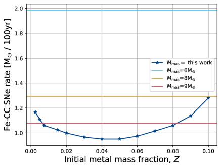
Figure 7: Here, we show estimates for Fe CCSNe rates (calculated using Equation. 14) for metallicity independent $M_{\rm mas}$ values (6, 8 and 9$M_{\odot}$) and the metallicity dependent $M_{\rm mas}$ values derived in this work. This figure is produced using the following values and prescriptions: we use a standard Salpeter IMF (Salpeter, 1955) of $\phi(m)=m^{-2.35}$ for a galactic population with masses between 0.1$M_{\odot}$ ($m_{L}$) and 100$M_{\odot}$ ($m_{U}$). We set $m_{u}^{\rm CC}=40$$M_{\odot}$ and $m_{l}^{\rm CC}=M_{\rm mas}$ as a function of $Z$ and use a value of $\psi(z)=1.9$$M_{\odot}$yr^-1 (based on estimates of the Milky Way SFR; Chomiuk & Povich 2011; Kennicutt Jr & Evans 2012). As stated in the text, we caution the reader that this is purely an example of how using metallicity dependent $M_{\rm mas}$ can influence the Fe CCSNe rate, using rough estimates for the other values in Equation. 14. These rates need to be considered more thoroughly before being used for quantitative purposes.

To produce Figure 7, we use a standard Salpeter IMF (Salpeter, 1955) of $\phi(m)=m^{-2.35}$ for a galactic population with masses between 0.1$M_{\odot}$ ($m_{L}$) and 100$M_{\odot}$ ($m_{U}$). We set $m_{u}^{\rm CC}=40$$M_{\odot}$ and $m_{l}^{\rm CC}=M_{\rm mas}$ as a function of $Z$ and use a value of $\psi(z)=1.9$$M_{\odot}$yr^-1 (roughly appropriate for Milky Way star formation; Chomiuk & Povich 2011; Kennicutt Jr & Evans 2012). We emphasize here that the example presented in this Figure was calculated using rough estimates for the other values in Equation 14 to serve purely as an example of how using metallicity–dependent $M_{\rm mas}$ can influence the Fe CCSNe rate. In reality, there are large uncertainties, and the inadequacy of using one constant value or prescription to model the diverse population of stars within a given galaxy is well established (see e.g. Jeřábková et al. 2018; Zhang et al. 2018; Hopkins 2018; Martín-Navarro et al. 2021 for IMFs, Heger et al. 2003 for final fate upper mass bounds and Chomiuk & Povich 2011; Kennicutt Jr & Evans 2012 for SFRs.) In any case, there is a notable difference between the Fe CCSNe rates calculated using metallicity–dependent $M_{\rm mas}$ values versus those using a fixed (Z-independent) $M_{\rm mas}$. For example, if we compare our curve to the constant SNe rate using $M_{\rm mas}=8$, we discern a 30% deviation between the two at $Z\sim 0.04$. Even close to solar metallicity ($Z=0.015$), the deviation is still 23%. The smallest variation is actually found at $Z=0.10$, where the difference between the two curves is less than 1%.

Beyond Fe CCSNe rates, the metallicity dependence of $M_{\rm mas}$ also has implications for theoretical galactic chemical evolution (GCE) simulations (for reviews on the topic of chemical evolution in galaxies, see e.g. Matteucci & Greggio 1986; Matteucci 1986, 2012; Wheeler & Sneden 1989; Kobayashi et al. 2020; Romano 2022). Consider $M_{i}$, the amount of available gas within a given galaxy comprising the chemical element $i$. For given $i$, we can use an equation for GCE (e.g. their Equation 4.1 in Matteucci 2012) to calculate $\dot{M}_{i}(t)$; i.e., the rate of change of $M_{i}$ within the galaxy. To perform this calculation, we consider how much $M_{i}$ is lost from the interstellar medium to form stars or through galactic winds, how much $M_{i}$ is then expelled from those stars and returned to the interstellar medium over their lifetimes (via stellar mass loss, binary interactions and SNe), as well as the composition–specific mass $M_{i}$ gained from gas infall. As we have emphasized in this work, the quantity and chemical composition of the gas expelled from a star over its lifetime is heavily dependent on the initial mass of the star. As such, achieving the correct integral bounds for the terms in Equation 4.1 from Matteucci (2012), which ultimately governs how much $M_{i}$ is returned to the ISM, is critical.

8 Conclusions

In this study, we have calculated $M_{\rm mas}$, the minimum initial mass required for stars to undergo a Fe CCSNe event, as a function of initial metallicity and presented the first results for super metal-rich models ($Z_{\rm max}=0.10$). We find that for the metallicity range $Z\approx 1\times 10^{-3}$ to $Z\approx 0.04$, the impact of increasing $\kappa$ with $Z$ results in lower $T_{\rm eff}$ and $L$ for their entire evolution. Higher initial masses are then required to ignite core C burning and undergo Fe CCSNe. At approximately $Z=0.05$, we find there is a reversal in this trend, where the impact of increasing $\mu$ with $Z$ begins to dominate. These—most metal-rich models—experience greater $T_{\rm eff}$ and $L$ on the main sequence and produce more massive H exhausted cores. Thus, $M_{\rm mas}$ begins to decline here as $Z$ extends to $Z=0.10$. These results rely on the linear scaling of initial He with $Z$. Our results imply that galactic evolution models are under–predicting SNe rates in the most metal–rich regions if using an extrapolation of a metallicity dependent curve (such as Ibeling & Heger 2013). We caution that the use of non-metallicity-dependent approximations do not reflect the sensitivity of $M_{\rm mas}$ to (even small changes in) $Z$. As such, they are inappropriate, particularly for chemical evolution studies of spiral galaxies and giant ellipticals with metal-rich regions.

Data Availability

MESA, the software used to produce the simulations for this paper, is a fully open-source stellar evolution code available at https://github.com/MESAHub/. Following the best practices of the MESA community, data and inlists required to reproduce our results are publicly available at 10.5281/zenodo.8237700.

Appendix A Other figures

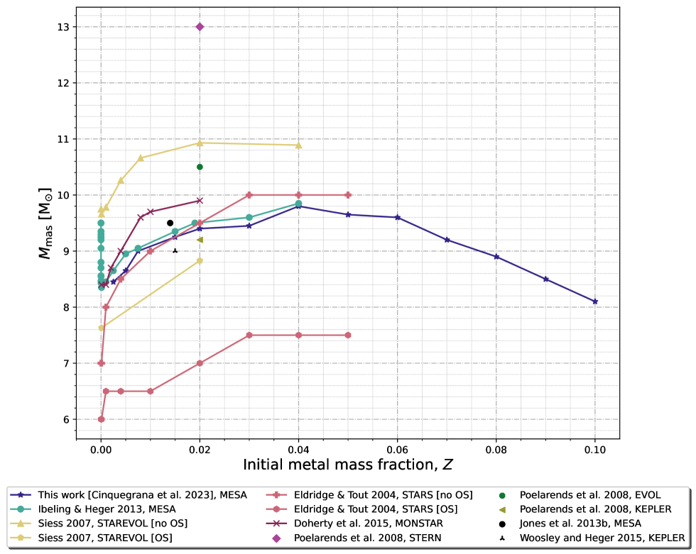
Figure 8: A comparison of our calculated $M_{\rm mas}$ against that currently available in the literature, where $M_{\rm mas}$ is the minimum initial mass required for a star to undergo an Fe CCSNe. The relevant input physics used in each set of models, where available, is listed in Table. 3.

References

- Agrawal et al. (2022) Agrawal P., Szécsi D., Stevenson S., Eldridge J. J., Hurley J., 2022, Monthly Notices of the Royal Astronomical Society, 512, 5717
- Aguirre et al. (2020) Aguirre V. S., et al., 2020, Astronomy & Astrophysics, 635, A164
- Althaus et al. (2003) Althaus L. G., Serenelli A. M., Córsico A. H., Montgomery M. H., 2003, A&A, 404, 593
- Anders et al. (2022) Anders E. H., Jermyn A. S., Lecoanet D., Fraser A. E., Cresswell I. G., Joyce M., Fuentes J., 2022, The Astrophysical Journal Letters, 928, L10
- Angelou et al. (2015) Angelou G. C., D’Orazi V., Constantino T. N., Church R. P., Stancliffe R. J., Lattanzio J. C., 2015, Monthly Notices of the Royal Astronomical Society, 450, 2423
- Angulo et al. (1999) Angulo C., et al., 1999, Nuclear Physics A, 656, 3
- Aver et al. (2013) Aver E., Olive K. A., Porter R., Skillman E. D., 2013, Journ. of Cosm. and Astroparticle Physics, 2013, 017
- Bahcall et al. (1995) Bahcall J. N., Pinsonneault M., Wasserburg G., 1995, Reviews of Modern Physics, 67, 781
- Balser (2006) Balser D. S., 2006, The Astronomical Journal, 132, 2326
- Bennett et al. (2012) Bennett M., et al., 2012, Monthly Notices of the Royal Astronomical Society, 420, 3047
- Bensby et al. (2017) Bensby T., et al., 2017, A&A, 605, A89
- Bersten et al. (2011) Bersten M. C., Benvenuto O., Hamuy M., 2011, The Astrophysical Journal, 729, 61
- Bertelli Motta et al. (2018) Bertelli Motta C., et al., 2018, MNRAS, 478, 425
- Bertelli et al. (2008) Bertelli G., Girardi L., Marigo P., Nasi E., 2008, A & A, 484, 815
- Blöcker (1995) Blöcker T., 1995, A&AS, 297, 727
- Blöcker et al. (1998) Blöcker T., Holweger H., Freytag B., Herwig F., Ludwig H.-G., Steffen M., 1998, Solar Composition and Its Evolution—From Core to Corona, pp 105–112
- Boehm-Vitense (1979) Boehm-Vitense E., 1979, ApJ, 234, 521
- Bohm & Cassinelli (1971) Bohm K., Cassinelli J., 1971, Astronomy and Astrophysics, 12, 21
- Böhm-Vitense (1958) Böhm-Vitense E., 1958, Zeitschrift fur Astrophysik, 46, 108
- Bono et al. (1997) Bono G., Caputo F., Cassisi S., Castellani V., Marconi M., 1997, The Astrophysical Journal, 489, 822
- Bono et al. (2000) Bono G., Caputo F., Cassisi S., Marconi M., Piersanti L., Tornambè A., 2000, ApJ, 543, 955
- Bossini et al. (2015) Bossini D., et al., 2015, Monthly Notices of the Royal Astronomical Society, 453, 2290
- Botticella et al. (2008) Botticella M., et al., 2008, Astronomy & Astrophysics, 479, 49
- Botticella et al. (2012) Botticella M., Smartt S., Kennicutt R., Cappellaro E., Sereno M., Lee J., 2012, Astronomy & Astrophysics, 537, A132
- Bravo et al. (2011) Bravo E., Piersanti L., Domínguez I., Straniero O., Isern J., Escartin J., 2011, Astronomy & Astrophysics, 535, A114
- Bressan et al. (1981) Bressan A., Chiosi C., Bertelli G., 1981, Astronomy and Astrophysics, 102, 25
- Bressan et al. (1993) Bressan A., Fagotto F., Bertelli G., Chiosi C., 1993, Astronomy and Astrophysics Supplement Series, 100, 647
- Brogaard et al. (2012) Brogaard K., et al., 2012, Astronomy & Astrophysics, 543, A106
- Campbell (2007) Campbell S. W., 2007, PhD thesis, Monash University
- Campilho et al. (2022) Campilho B., Deal M., Bossini D., 2022, arXiv preprint arXiv:2201.03439
- Canuto & Mazzitelli (1991) Canuto V., Mazzitelli I., 1991, ApJ, 370, 295
- Canuto et al. (1996) Canuto V., Goldman I., Mazzitelli I., 1996, The Astrophysical Journal, 473, 550
- Cappellaro et al. (1996) Cappellaro E., Turatto M., Tsvetkov D. Y., Bartunov O., Pollas C., Evans R., Hamuy M., 1996, arXiv preprint astro-ph/9611191
- Carbon et al. (1982) Carbon D. F., Langer G., Butler D., Kraft R., Suntzeff N., Kemper E., Trefzger C. F., Romanishin W., 1982, The Astrophysical Journal Supplement Series, 49, 207
- Casagrande et al. (2007a) Casagrande L., Flynn C., Portinari L., Girardi L., Jimenez R., 2007a, MNRAS, 382, 1516
- Casagrande et al. (2007b) Casagrande L., Flynn C., Portinari L., Girardi L., Jimenez R., 2007b, Monthly Notices of the Royal Astronomical Society, 382, 1516
- Castellani et al. (1997) Castellani V., Ciacio F., Degl’Innocenti S., Fiorentini G., 1997, arXiv preprint astro-ph/9705035
- Caughlan & Fowler (1988) Caughlan G. R., Fowler W. A., 1988, Atomic Data and Nuclear Data Tables, 40, 283
- Chaboyer et al. (2001) Chaboyer B., Fenton W., Nelan J. E., Patnaude D., Simon F. E., 2001, The Astrophysical Journal, 562, 521
- Chandrasekhar (1935) Chandrasekhar S., 1935, Monthly Notices of the Royal Astronomical Society, 95, 207
- Charbonnel (1994) Charbonnel C., 1994, Astronomy and Astrophysics, 282, 811
- Charbonnel & Lagarde (2010) Charbonnel C., Lagarde N., 2010, Astronomy & Astrophysics, 522, A10
- Charbonnel & Zahn (2007) Charbonnel C., Zahn J.-P., 2007, Astronomy & Astrophysics, 467, L15
- Charbonnel & do Nascimento Jr (1998) Charbonnel C., do Nascimento Jr J., 1998, arXiv preprint astro-ph/9805235
- Chen et al. (2014) Chen M. C., Herwig F., Denissenkov P. A., Paxton B., 2014, Monthly Notices of the Royal Astronomical Society, 440, 1274
- Chiappini et al. (2002) Chiappini C., Renda A., Matteucci F., 2002, Astronomy & Astrophysics, 395, 789
- Chieffi et al. (1998) Chieffi A., Limongi M., Straniero O., 1998, The Astrophysical Journal, 502, 737
- Choi et al. (2016) Choi J., Dotter A., Conroy C., Cantiello M., Paxton B., Johnson B. D., 2016, ApJ, 823, 102
- Choi et al. (2018) Choi J., Dotter A., Conroy C., Ting Y.-S., 2018, ApJ, 860, 131
- Chomiuk & Povich (2011) Chomiuk L., Povich M. S., 2011, The Astronomical Journal, 142, 197
- Christensen-Dalsgaard (2008) Christensen-Dalsgaard J., 2008, Ap&SS, 316, 13
- Cinquegrana & Joyce (2022) Cinquegrana G. C., Joyce M., 2022, Research Notes of the AAS, 6, 77
- Cinquegrana & Karakas (2022) Cinquegrana G. C., Karakas A. I., 2022, Monthly Notices of the Royal Astronomical Society, 510, 1557
- Cinquegrana et al. (2022) Cinquegrana G. C., Joyce M., Karakas A. I., 2022, arXiv e-prints, p. arXiv:2208.01859
- Claret (2007) Claret A., 2007, A&AS, 467, 1389
- Cohen et al. (2003) Cohen J. G., Blakeslee J., Côté P., 2003, ApJ, 592, 866
- Constantino et al. (2015) Constantino T., Campbell S. W., Christensen-Dalsgaard J., Lattanzio J. C., Stello D., 2015, Monthly Notices of the Royal Astronomical Society, 452, 123
- Cox & Giuli (1968) Cox J., Giuli R., 1968, New York
- Curto et al. (2010) Curto G. L., et al., 2010, Astronomy & Astrophysics, 512, A48
- Cyburt et al. (2010) Cyburt R. H., et al., 2010, ApJ Supp. Ser., 189, 240
- Davies & Beasor (2018) Davies B., Beasor E. R., 2018, Monthly Notices of the Royal Astronomical Society, 474, 2116
- Deal et al. (2018) Deal M., Alecian G., Lebreton Y., Goupil M., Marques J., LeBlanc F., Morel P., Pichon B., 2018, Astronomy & Astrophysics, 618, A10
- Demarque et al. (2008) Demarque P., Guenther D., Li L., Mazumdar A., Straka C., 2008, Astrophysics and Space Science, 316, 31
- Denissenkov & Tout (2003) Denissenkov P. A., Tout C. A., 2003, Monthly Notices of the Royal Astronomical Society, 340, 722
- Dessart et al. (2010) Dessart L., Livne E., Waldman R., 2010, Monthly Notices of the Royal Astronomical Society, 408, 827
- Díaz-Rodríguez et al. (2018) Díaz-Rodríguez M., Murphy J. W., Rubin D. A., Dolphin A. E., Williams B. F., Dalcanton J. J., 2018, The Astrophysical Journal, 861, 92
- Díaz-Rodríguez et al. (2021) Díaz-Rodríguez M., Murphy J. W., Williams B. F., Dalcanton J. J., Dolphin A. E., 2021, Monthly Notices of the Royal Astronomical Society, 506, 781
- Do et al. (2015a) Do T., Kerzendorf W., Winsor N., Støstad M., Morris M. R., Lu J. R., Ghez A. M., 2015a, ApJ, 809, 143
- Do et al. (2015b) Do T., Kerzendorf W., Winsor N., Støstad M., Morris M. R., Lu J. R., Ghez A. M., 2015b, The Astrophysical Journal, 809, 143
- Dobbie et al. (2006) Dobbie P., et al., 2006, Monthly Notices of the Royal Astronomical Society, 369, 383
- Doherty (2014) Doherty C. L., 2014, PhD thesis, Monash University
- Doherty et al. (2015) Doherty C. L., Gil-Pons P., Siess L., Lattanzio J. C., Lau H. H., 2015, Monthly Notices of the Royal Astronomical Society, 446, 2599
- Doherty et al. (2017) Doherty C. L., Gil-Pons P., Siess L., Lattanzio J. C., 2017, Publications of the Astronomical Society of Australia, 34
- Dotter et al. (2007) Dotter A., Chaboyer B., Jevremović D., Baron E., Ferguson J. W., Sarajedini A., Anderson J., 2007, The Astronomical Journal, 134, 376
- Eggenberger et al. (2008) Eggenberger P., Meynet G., Maeder A., Hirschi R., Charbonnel C., Talon S., Ekström S., 2008, Astrophysics and Space Science, 316, 43
- Eggleton (1971) Eggleton P. P., 1971, Monthly Notices of the Royal Astronomical Society, 151, 351
- Eifler et al. (2021) Eifler T., et al., 2021, Monthly Notices of the Royal Astronomical Society, 507, 1514
- Eldridge & Tout (2004) Eldridge J. J., Tout C., 2004, Monthly Notices of the Royal Astronomical Society, 353, 87
- Eldridge et al. (2017) Eldridge J., Stanway E., Xiao L., McClelland L., Taylor G., Ng M., Greis S., Bray J., 2017, Publications of the Astronomical Society of Australia, 34
- Elias-Rosa et al. (2009) Elias-Rosa N., et al., 2009, The Astrophysical Journal, 706, 1174
- Fagotto et al. (1994) Fagotto F., Bressan A., Bertelli G., Chiosi C., 1994, Astronomy and Astrophysics Supplement Series, 105, 39
- Fahrion et al. (2020) Fahrion K., et al., 2020, Astronomy & Astrophysics, 637, A27
- Farmer et al. (2016) Farmer R., Fields C., Petermann I., Dessart L., Cantiello M., Paxton B., Timmes F., 2016, The Astrophysical Journal Supplement Series, 227, 22
- Farmer et al. (2019) Farmer R., Renzo M., de Mink S., Marchant P., Justham S., 2019, The Astrophysical Journal, 887, 53
- Faulkner (1967) Faulkner J., 1967, The Astrophysical Journal, 147, 617
- Feltzing & Chiba (2013) Feltzing S., Chiba M., 2013, New Astron. Rev., 57, 80
- Fernandes et al. (1996) Fernandes J., Lebreton Y., Baglin A., 1996, Astronomy and Astrophysics, 311, 127
- Fields et al. (2018) Fields C., Timmes F., Farmer R., Petermann I., Wolf W. M., Couch S., 2018, The Astrophysical Journal Supplement Series, 234, 19
- Forestini (1994) Forestini M., 1994, Astronomy and Astrophysics, 285, 473
- Fraser et al. (2011) Fraser M., et al., 2011, Monthly Notices of the Royal Astronomical Society, 417, 1417
- Fraser et al. (2022) Fraser A. E., Joyce M., Anders E. H., Tayar J., Cantiello M., 2022, The Astrophysical Journal, 941, 164
- Freytag et al. (1996) Freytag B., Ludwig H.-G., Steffen M., 1996, Astronomy and Astrophysics, 313, 497
- Frost & Lattanzio (1996) Frost C., Lattanzio J., 1996, ApJ, 473, 383
- Fuller et al. (1985) Fuller G., Fowler W., Newman M., 1985, The Astrophysical Journal, 293, 1
- Gabriel (1997) Gabriel M., 1997, arXiv preprint astro-ph/9706213
- Gabriel et al. (2014) Gabriel M., Noels A., Montalban J., Miglio A., 2014, Astronomy & Astrophysics, 569, A63
- Gaia Collaboration et al. (2021) Gaia Collaboration et al., 2021, A&A, 649, A1
- Garaud (2018) Garaud P., 2018, Annual Review of Fluid Mechanics, 50, 275
- Garaud (2021) Garaud P., 2021, in , Multi-Dimensional Processes in Stellar Physics. EDP Sciences, pp 13–60
- Garcia Lopez & Spruit (1991) Garcia Lopez R. J., Spruit H. C., 1991, The Astrophysical Journal, 377, 268
- Gardner et al. (2006) Gardner J. P., et al., 2006, Space Science Reviews, 123, 485
- Gasques et al. (2007) Gasques L., Brown E., Chieffi A., Jiang C., Limongi M., Rolfs C., Wiescher M., Yakovlev D., 2007, Physical Review C, 76, 035802
- Genel et al. (2014) Genel S., et al., 2014, Monthly Notices of the Royal Astronomical Society, 445, 175
- Gennaro et al. (2010) Gennaro M., Moroni P. P., Degl’Innocenti S., 2010, Astronomy & Astrophysics, 518, A13
- Gilroy (1989) Gilroy K. K., 1989, The Astrophysical Journal, 347, 835
- Girardi et al. (2002) Girardi L., Bertelli G., Bressan A., Chiosi C., Groenewegen M., Marigo P., Salasnich B., Weiss A., 2002, Astronomy & Astrophysics, 391, 195
- Gogarten et al. (2009a) Gogarten S. M., et al., 2009a, The Astrophysical Journal, 691, 115
- Gogarten et al. (2009b) Gogarten S. M., Dalcanton J. J., Murphy J. W., Williams B. F., Gilbert K., Dolphin A., 2009b, The Astrophysical Journal, 703, 300
- Gratton et al. (2000) Gratton R., Sneden C., Carretta E., Bragaglia A., 2000, Astronomy and Astrophysics, 354, 169
- Heger et al. (2000) Heger A., Langer N., Woosley S., 2000, The Astrophysical Journal, 528, 368
- Heger et al. (2003) Heger A., Fryer C. L., Woosley S. E., Langer N., Hartmann D. H., 2003, The Astrophysical Journal, 591, 288
- Henkel et al. (2017) Henkel K., Karakas A. I., Lattanzio J. C., 2017, Monthly Notices of the Royal Astronomical Society, 469, 4600
- Henney & Ulrich (1995) Henney C., Ulrich R., 1995, Helioseismology, 376, 3
- Henyey et al. (1965) Henyey L., Vardya M., Bodenheimer P., 1965, The Astrophysical Journal, 142, 841
- Herwig (2000) Herwig F., 2000, arXiv preprint astro-ph/0007139
- Herwig (2004) Herwig F., 2004, The Astrophysical Journal, 605, 425
- Herwig & Austin (2004) Herwig F., Austin S. M., 2004, The Astrophysical Journal, 613, L73
- Herwig et al. (2006) Herwig F., Austin S. M., Lattanzio J. C., 2006, Physical Review C, 73, 025802
- Hidalgo et al. (2018) Hidalgo S. L., et al., 2018, The Astrophysical Journal, 856, 125
- Hopkins (2018) Hopkins A. M., 2018, Publications of the Astronomical Society of Australia, 35, e039
- Horiuchi et al. (2011) Horiuchi S., Beacom J. F., Kochanek C. S., Prieto J. L., Stanek K., Thompson T. A., 2011, The Astrophysical Journal, 738, 154
- Ibeling & Heger (2013) Ibeling D., Heger A., 2013, The Astrophysical Journal Letters, 765, L43
- Iben & Renzini (1983) Iben I., Renzini A., 1983, Annual review of Astronomy and Astrophysics, 21, 271
- Iglesias & Rogers (1996) Iglesias C. A., Rogers F. J., 1996, ApJ, 464, 943
- Irwin (2004) Irwin A. W., 2004, The FreeEOS Code for Calculating the Equation of State for Stellar Interiors, http://freeeos.sourceforge.net/
- Izotov et al. (2007) Izotov Y. I., Thuan T. X., Stasińska G., 2007, The Astrophysical Journal, 662, 15
- Izzard et al. (2007) Izzard R. G., Lugaro M., Karakas A. I., Iliadis C., van Raai M., 2007, A&A, 466, 641
- Jennings et al. (2012) Jennings Z. G., Williams B. F., Murphy J. W., Dalcanton J. J., Gilbert K. M., Dolphin A. E., Fouesneau M., Weisz D. R., 2012, The Astrophysical Journal, 761, 26
- Jennings et al. (2014) Jennings Z. G., Williams B. F., Murphy J. W., Dalcanton J. J., Gilbert K. M., Dolphin A. E., Weisz D. R., Fouesneau M., 2014, The Astrophysical Journal, 795, 170
- Jeřábková et al. (2018) Jeřábková T., Zonoozi A. H., Kroupa P., Beccari G., Yan Z., Vazdekis A., Zhang Z.-Y., 2018, Astronomy & Astrophysics, 620, A39
- Jerkstrand et al. (2012) Jerkstrand A., Fransson C., Maguire K., Smartt S., Ergon M., Spyromilio J., 2012, Astronomy & Astrophysics, 546, A28
- Jermyn et al. (2021) Jermyn A. S., Schwab J., Bauer E., Timmes F., Potekhin A. Y., 2021, The Astrophysical Journal, 913, 72
- Jermyn et al. (2022) Jermyn A. S., et al., 2022, arXiv e-prints, pp arXiv–2208
- Jiang et al. (2007) Jiang C., Rehm K., Back B., Janssens R., 2007, Physical Review C, 75, 015803
- Jimenez et al. (2003) Jimenez R., Flynn C., MacDonald J., Gibson B. K., 2003, Science, 299, 1552
- Jones et al. (2013) Jones S., et al., 2013, The Astrophysical Journal, 772, 150
- Jones et al. (2014) Jones S., Hirschi R., Nomoto K., 2014, The Astrophysical Journal, 797, 83
- Jones et al. (2015) Jones S., Hirschi R., Pignatari M., Heger A., Georgy C., Nishimura N., Fryer C., Herwig F., 2015, Monthly Notices of the Royal Astronomical Society, 447, 3115
- Jones et al. (2016) Jones S., Andrassy R., Sandalski S., Davis A., Woodward P., Herwig F., 2016, Monthly Notices of the Royal Astronomical Society, p. stw2783
- Joyce & Chaboyer (2015) Joyce M., Chaboyer B., 2015, ApJ, 814, 142
- Joyce & Chaboyer (2018a) Joyce M., Chaboyer B., 2018a, The Astrophysical Journal, 856, 10
- Joyce & Chaboyer (2018b) Joyce M., Chaboyer B., 2018b, The Astrophysical Journal, 864, 99
- Joyce & Tayar (2023) Joyce M., Tayar J., 2023, arXiv e-prints, p. arXiv:2303.09596
- Joyce et al. (2022) Joyce M., Johnson C. I., Marchetti T., Rich R. M., Simion I., Bourke J., 2022, arXiv e-prints, p. arXiv:2205.07964
- Joyce et al. (2023) Joyce M., Johnson C. I., Marchetti T., Rich R. M., Simion I., Bourke J., 2023, ApJ, 946, 28
- Kaiser et al. (2020) Kaiser E. A., Hirschi R., Arnett W. D., Georgy C., Scott L. J., Cristini A., 2020, Monthly Notices of the Royal Astronomical Society, 496, 1967
- Kamath et al. (2012) Kamath D., Karakas A. I., Wood P. R., 2012, The Astrophysical Journal, 746, 20
- Karakas (2010) Karakas A. I., 2010, in , Principles and Perspectives in Cosmochemistry. Springer, pp 107–164
- Karakas (2014) Karakas A. I., 2014, MNRAS, 445, 347
- Karakas & Lugaro (2016) Karakas A. I., Lugaro M., 2016, ApJ, 825, 26
- Karakas et al. (2006) Karakas A. I., Lugaro M. A., Wiescher M., Görres J., Ugalde C., 2006, ApJ, 643, 471
- Karakas et al. (2022) Karakas A. I., Cinquegrana G., Joyce M., 2022, Monthly Notices of the Royal Astronomical Society, 509, 4430
- Kato (1966) Kato S., 1966, Publications of the Astronomical Society of Japan, 18, 374
- Keane & Kramer (2008) Keane E. F., Kramer M., 2008, Monthly Notices of the Royal Astronomical Society, 391, 2009
- Kennicutt Jr & Evans (2012) Kennicutt Jr R. C., Evans N. J., 2012, Annual Review of Astronomy and Astrophysics, 50, 531
- Kippenhahn et al. (1980) Kippenhahn R., Ruschenplatt G., Thomas H.-C., 1980, Astronomy and Astrophysics, 91, 175
- Kippenhahn et al. (2012) Kippenhahn R., Weigert A., Weiss A., 2012, Stellar structure and evolution. Springer
- Kobayashi et al. (2020) Kobayashi C., Karakas A. I., Lugaro M., 2020, The Astrophysical Journal, 900, 179
- Kraft (1994) Kraft R. P., 1994, Publications of the Astronomical Society of the Pacific, 106, 553
- Kurucz (1979) Kurucz R. L., 1979, The Astrophysical Journal Supplement Series, 40, 1
- LSST Science Collaboration et al. (2017) LSST Science Collaboration et al., 2017, preprint, (arXiv:1708.04058)
- Lagarde et al. (2011) Lagarde N., Charbonnel C., Decressin T., Hagelberg J., 2011, Astronomy & Astrophysics, 536, A28
- Lagarde et al. (2012) Lagarde N., Romano D., Charbonnel C., Tosi M., Chiappini C., Matteucci F., 2012, Astronomy & Astrophysics, 542, A62
- Langanke & Martınez-Pinedo (2000) Langanke K., Martınez-Pinedo G., 2000, Nuclear Physics A, 673, 481
- Langer (1998) Langer N., 1998, Astronomy and Astrophysics, 329, 551
- Langer et al. (1985) Langer N., El Eid M., Fricke K., 1985, Astronomy and Astrophysics, 145, 179
- Laplace et al. (2021) Laplace E., Justham S., Renzo M., Götberg Y., Farmer R., Vartanyan D., de Mink S., 2021, arXiv preprint arXiv:2102.05036
- Lattanzio (1986) Lattanzio J. C., 1986, ApJ, 311, 708
- Lattanzio et al. (2015) Lattanzio J. C., Siess L., Church R. P., Angelou G., Stancliffe R. J., Doherty C. L., Stephen T., Campbell S. W., 2015, Monthly Notices of the Royal Astronomical Society, 446, 2673
- Lépine et al. (2011) Lépine J. R., et al., 2011, MNRAS, 417, 698
- Li et al. (2011) Li W., Chornock R., Leaman J., Filippenko A. V., Poznanski D., Wang X., Ganeshalingam M., Mannucci F., 2011, Monthly Notices of the Royal Astronomical Society, 412, 1473
- Limongi & Chieffi (2006) Limongi M., Chieffi A., 2006, The Astrophysical Journal, 647, 483
- Limongi & Chieffi (2020) Limongi M., Chieffi A., 2020, The Astrophysical Journal, 902, 95
- Liu et al. (2019) Liu F., Asplund M., Yong D., Feltzing S., Dotter A., Meléndez J., Ramírez I., 2019, A&A, 627, A117
- Lodders (2003) Lodders K., 2003, ApJ, 591, 1220
- Lugaro et al. (2004) Lugaro M., Ugalde C., Karakas A. I., Görres J., Wiescher M., Lattanzio J. C., Cannon R. C., 2004, The Astrophysical Journal, 615, 934
- Magg et al. (2022) Magg E., et al., 2022, Astronomy & Astrophysics, 661, A140
- Marchant et al. (2019) Marchant P., Renzo M., Farmer R., Pappas K. M., Taam R. E., De Mink S. E., Kalogera V., 2019, The Astrophysical Journal, 882, 36
- Marigo & Aringer (2009) Marigo P., Aringer B., 2009, A&A, 508, 1539
- Marigo et al. (2008) Marigo P., Girardi L., Bressan A., Groenewegen M. A., Silva L., Granato G. L., 2008, Astronomy & Astrophysics, 482, 883
- Marigo et al. (2013) Marigo P., Bressan A., Nanni A., Girardi L., Pumo M. L., 2013, Mon. Notes R. Astron. Soc., 434, 488
- Marigo et al. (2017) Marigo P., et al., 2017, ApJ, 835, 77
- Marques et al. (2013) Marques J., et al., 2013, Astronomy & Astrophysics, 549, A74
- Martig et al. (2015) Martig M., et al., 2015, Monthly Notices of the Royal Astronomical Society, 451, 2230
- Martín-Navarro et al. (2021) Martín-Navarro I., et al., 2021, Astronomy & Astrophysics, 654, A59
- Martinez & Bersten (2019) Martinez L., Bersten M. C., 2019, Astronomy & Astrophysics, 629, A124
- Martins & Palacios (2013) Martins F., Palacios A., 2013, Astronomy & Astrophysics, 560, A16
- Matteucci (1986) Matteucci F., 1986, Publications of the Astronomical Society of the Pacific, 98, 973
- Matteucci (2012) Matteucci F., 2012, Chemical evolution of galaxies. Springer Science & Business Media
- Matteucci & Greggio (1986) Matteucci F., Greggio L., 1986, Astronomy and Astrophysics, 154, 279
- Maund et al. (2011) Maund J., et al., 2011, The Astrophysical Journal Letters, 739, L37
- McDonald & Zijlstra (2015) McDonald I., Zijlstra A., 2015, Monthly Notices of the Royal Astronomical Society, 448, 502
- McWilliam & Rich (1994) McWilliam A., Rich R. M., 1994, The Astrophysical Journal Supplement Series, 91, 749
- Mena et al. (2017) Mena E. D., Tsantaki M., Adibekyan V. Z., Sousa S., Santos N., Hernández J. G., Israelian G., 2017, Astronomy & Astrophysics, 606, A94
- Meynet et al. (2006) Meynet G., Mowlavi N., Maeder A., 2006, ArX. Pre. astro-ph/0611261
- Mihalas (1978) Mihalas D., 1978, San Francisco: WH Freeman
- Mihalas et al. (1978) Mihalas D., Auer L., Mihalas B., 1978, The Astrophysical Journal, 220, 1001
- Mirouh et al. (2012) Mirouh G. M., Garaud P., Stellmach S., Traxler A. L., Wood T. S., 2012, The Astrophysical Journal, 750, 61
- Miyaji et al. (1980) Miyaji S., Nomoto K., Yokoi K., Sugimoto D., 1980, Publications of the Astronomical Society of Japan, 32, 303
- Moll et al. (2016) Moll R., Garaud P., Stellmach S., 2016, The Astrophysical Journal, 823, 33
- Monpribat et al. (2022) Monpribat E., et al., 2022, Astronomy & Astrophysics, 660, A47
- Moore & Garaud (2016) Moore K., Garaud P., 2016, The Astrophysical Journal, 817, 54
- Morel & Lebreton (2008) Morel P., Lebreton Y., 2008, Ap&SS, 316, 61
- Mowlavi et al. (1998a) Mowlavi N., Schaerer D., Meynet G., Bernasconi P., Charbonnel C., Maeder A., 1998a, Astronomy and Astrophysics Supplement Series, 128, 471
- Mowlavi et al. (1998b) Mowlavi N., Meynet G., Maeder A., Schaerer D., Charbonnel C., 1998b, Astronomy and Astrophysics, 335, 573
- Naiman et al. (2018) Naiman J. P., et al., 2018, Monthly Notices of the Royal Astronomical Society, 477, 1206
- Ness & Freeman (2016) Ness M., Freeman K., 2016, Publications of the Astronomical Society of Australia, 33, e022
- Nomoto (1984) Nomoto K., 1984, The Astrophysical Journal, 277, 791
- Oda et al. (1994) Oda T., Hino M., Muto K., Takahara M., Sato K., 1994, Atomic Data and Nuclear Data Tables, 56, 231
- PHASE (2003) PHASE C., 2003, The Messenger, 114, 20
- Pagel & Portinari (1998) Pagel B., Portinari L., 1998, Monthly Notices of the Royal Astronomical Society, 298, 747
- Palacios et al. (2003) Palacios A., Talon S., Charbonnel C., Forestini M., 2003, Astronomy & Astrophysics, 399, 603
- Paxton et al. (2010) Paxton B., Bildsten L., Dotter A., Herwig F., Lesaffre P., Timmes F., 2010, The Astrophysical Journal Supplement Series, 192, 3
- Paxton et al. (2013) Paxton B., et al., 2013, The Astrophysical Journal Supplement Series, 208, 4
- Paxton et al. (2015) Paxton B., et al., 2015, The Astrophysical Journal Supplement Series, 220, 15
- Paxton et al. (2018) Paxton B., et al., 2018, The Astrophysical Journal Supplement Series, 234, 34
- Paxton et al. (2019) Paxton B., et al., 2019, The Astrophysical Journal Supplement Series, 243, 10
- Pedersen et al. (2021) Pedersen M. G., et al., 2021, Nature Astronomy, 5, 715
- Perrin et al. (1977) Perrin M.-N., Hejlesen P., Cayrel de Strobel G., Cayrel R., 1977, Astronomy and Astrophysics, 54, 779
- Pietrinferni et al. (2004) Pietrinferni A., Cassisi S., Salaris M., Castelli F., 2004, The Astrophysical Journal, 612, 168
- Pietrinferni et al. (2021) Pietrinferni A., et al., 2021, The Astrophysical Journal, 908, 102
- Pignatari et al. (2012) Pignatari M., et al., 2012, The Astrophysical Journal, 762, 31
- Pilachowski (1986) Pilachowski C., 1986, The Astrophysical Journal, 300, 289
- Pillepich et al. (2018) Pillepich A., et al., 2018, Monthly Notices of the Royal Astronomical Society, 473, 4077
- Pinsonneault et al. (2018) Pinsonneault M. H., et al., 2018, The Astrophysical Journal Supplement Series, 239, 32
- Poelarends et al. (2008) Poelarends A., Herwig F., Langer N., Heger A., 2008, The Astrophysical Journal, 675, 614
- Portinari et al. (2010) Portinari L., Casagrande L., Flynn C., 2010, Monthly Notices of the Royal Astronomical Society, 406, 1570
- Potekhin & Chabrier (2010) Potekhin A. Y., Chabrier G., 2010, Contributions to Plasma Physics, 50, 82
- Prandtl (1925) Prandtl L., 1925, Z. Angew. Math. Mech., 136
- Radko (2003) Radko T., 2003, Journal of Fluid Mechanics, 497, 365
- Reimers (1975) Reimers D., 1975, in , Problems in stellar atmospheres and envelopes. Springer, pp 229–256
- Renzini (1994) Renzini A., 1994, Astronomy and Astrophysics, 285
- Renzo et al. (2020a) Renzo M., Farmer R., Justham S., de Mink S., Götberg Y., Marchant P., 2020a, Monthly Notices of the Royal Astronomical Society, 493, 4333
- Renzo et al. (2020b) Renzo M., Farmer R., Justham S., Götberg Y., de Mink S., Zapartas E., Marchant P., Smith N., 2020b, Astronomy & Astrophysics, 640, A56
- Ribas et al. (2000) Ribas I., Jordi C., Torra J., Giménez Á., 2000, Monthly Notices of the Royal Astronomical Society, 313, 99
- Richer et al. (2000) Richer J., Michaud G., Turcotte S., 2000, The Astrophysical Journal, 529, 338
- Ricker et al. (2015) Ricker G. R., et al., 2015, Journal of Astronomical Telescopes, Instruments, and Systems, 1, 014003
- Rogers & Iglesias (1992) Rogers F. J., Iglesias C. A., 1992, ApJ Supp. Series, 79, 507
- Rogers & Nayfonov (2002) Rogers F. J., Nayfonov A., 2002, ApJ, 576, 1064
- Rogers et al. (2013) Rogers T., Lin D. N., McElwaine J., Lau H. H. B., 2013, The Astrophysical Journal, 772, 21
- Romano (2022) Romano D., 2022, The Astronomy and Astrophysics Review, 30, 1
- Rosenblum et al. (2011) Rosenblum E., Garaud P., Traxler A., Stellmach S., 2011, The Astrophysical Journal, 731, 66
- Roy et al. (2011) Roy R., et al., 2011, The Astrophysical Journal, 736, 76
- Ryde & Schultheis (2015) Ryde N., Schultheis M., 2015, Astronomy & Astrophysics, 573, A14
- Salaris et al. (2004) Salaris M., Riello M., Cassisi S., Piotto G., 2004, Astronomy & Astrophysics, 420, 911
- Salaris et al. (2022) Salaris M., Cassisi S., Pietrinferni A., Hidalgo S., 2022, Monthly Notices of the Royal Astronomical Society, 509, 5197
- Salasnich et al. (2000) Salasnich B., Girardi L., Weiss A., Chiosi C., 2000, A%A, 361, 1023
- Sallaska et al. (2013) Sallaska A. L., Iliadis C., Champange A., Goriely S., Starrfield S., Timmes F., 2013, The Astrophysical Journal Supplement Series, 207, 18
- Salpeter (1955) Salpeter E. E., 1955, ApJ, 121, 161
- Santos et al. (2011) Santos N., et al., 2011, Astronomy & Astrophysics, 526, A112
- Sarzi et al. (2018) Sarzi M., et al., 2018, A&A, 616, A121
- Saumon et al. (1995) Saumon D., Chabrier G., van Horn H. M., 1995, ApJS, 99, 713
- Schröder et al. (1997) Schröder K.-P., Pols O. R., Eggleton P. P., 1997, Monthly Notices of the Royal Astronomical Society, 285, 696
- Schwarzschild & Härm (1958) Schwarzschild M., Härm R., 1958, The Astrophysical Journal, 128, 348
- Scott et al. (2021) Scott L., Hirschi R., Georgy C., Arnett W., Meakin C., Kaiser E., Ekström S., Yusof N., 2021, Monthly Notices of the Royal Astronomical Society, 503, 4208
- Seaton (1995) Seaton M., 1995, Opacity Project Team 1995 The Opacity Project vol 1 and 2
- Semenova et al. (2020) Semenova E., et al., 2020, Astronomy & Astrophysics, 643, A164
- Shaviv & Salpeter (1973) Shaviv G., Salpeter E. E., 1973, The Astrophysical Journal, 184, 191
- Shetrone et al. (2019) Shetrone M., et al., 2019, The Astrophysical Journal, 872, 137
- Siess (2006) Siess L., 2006, Astronomy & Astrophysics, 448, 717
- Siess (2007a) Siess L., 2007a, A&AS, 476, 893
- Siess (2007b) Siess L., 2007b, Astronomy & astrophysics, 476, 893
- Siess et al. (1997) Siess L., Forestini M., Dougados C., 1997, Astronomy and Astrophysics, 324, 556
- Siess et al. (2000) Siess L., Dufour E., Forestini M., 2000, arXiv preprint astro-ph/0003477
- Sijacki et al. (2015) Sijacki D., Vogelsberger M., Genel S., Springel V., Torrey P., Snyder G. F., Nelson D., Hernquist L., 2015, Monthly Notices of the Royal Astronomical Society, 452, 575
- Skumanich (1972) Skumanich A., 1972, ApJ, 171, 565
- Smartt (2009) Smartt S. J., 2009, Annual Review of Astronomy and Astrophysics, 47, 63
- Smartt (2015) Smartt S., 2015, Publications of the Astronomical Society of Australia, 32
- Smartt et al. (2009) Smartt S., Eldridge J., Crockett R., Maund J., 2009, Monthly Notices of the Royal Astronomical Society, 395, 1409
- Spiegel (1969) Spiegel E., 1969, Comments on Astrophysics and Space Physics, 1, 57
- Spillane et al. (2007) Spillane T., et al., 2007, Physical Review Letters, 98, 122501
- Spiro et al. (2014) Spiro S., et al., 2014, Monthly Notices of the Royal Astronomical Society, 439, 2873
- Spruit (1992) Spruit H., 1992, Astronomy and Astrophysics, 253, 131
- Spruit (2013) Spruit H., 2013, Astronomy & Astrophysics, 552, A76
- Staritsin (2013) Staritsin E., 2013, Astronomy Reports, 57, 380
- Stern (1960) Stern M. E., 1960, Tellus, 12, 172
- Straniero et al. (2016) Straniero O., Piersanti L., Cristallo S., 2016, in Journal of Physics: Conference Series. p. 012008
- Sukhbold & Woosley (2014) Sukhbold T., Woosley S., 2014, The Astrophysical Journal, 783, 10
- Szécsi et al. (2022) Szécsi D., Agrawal P., Wünsch R., Langer N., 2022, Astronomy and Astrophysics, 658, A125
- Tayar & Joyce (2022) Tayar J., Joyce M., 2022, ApJ, 935, L30
- Tayar et al. (2022) Tayar J., Claytor Z. R., Huber D., van Saders J., 2022, ApJ, 927, 31
- Tayler (1954) Tayler R. J., 1954, ApJ, 120, 332
- Thomas (1967) Thomas H. C., 1967, Z. Astrophys., 67, 420
- Thorsbro et al. (2020) Thorsbro B., et al., 2020, The Astrophysical Journal, 894, 26
- Timmes & Swesty (2000) Timmes F. X., Swesty F. D., 2000, ApJS, 126, 501
- Tomasella et al. (2018) Tomasella L., et al., 2018, Monthly Notices of the Royal Astronomical Society, 475, 1937
- Tumino et al. (2021) Tumino A., Bertulani C. A., La Cognata M., Lamia L., Pizzone R. G., Romano S., Typel S., 2021, Annual Review of Nuclear and Particle Science, 71, 345
- Turcotte et al. (1998) Turcotte S., Richer J., Michaud G., Iglesias C., Rogers F., 1998, The Astrophysical Journal, 504, 539
- Ulrich (1972) Ulrich R. K., 1972, The Astrophysical Journal, 172, 165
- Utrobin (2007) Utrobin V. P., 2007, Astronomy & Astrophysics, 461, 233
- Valcarce et al. (2013a) Valcarce A. A. R., Catelan M., De Medeiros J. R., 2013a, A%A, 553
- Valcarce et al. (2013b) Valcarce A. A., Catelan M., De Medeiros J. R., 2013b, Astronomy & Astrophysics, 553, A62
- Van Den Bergh (1991) Van Den Bergh S., 1991, Physics reports, 204, 385
- Van Dyk et al. (2011) Van Dyk S. D., et al., 2011, The Astrophysical Journal Letters, 741, L28
- Van Raai et al. (2008) Van Raai M., Lugaro M., Karakas A. I., Iliadis C., 2008, Astronomy & Astrophysics, 478, 521
- Van den Bergh et al. (1987) Van den Bergh S., McClure R. D., Evans R., 1987, The Astrophysical Journal, 323, 44
- Varghese et al. (2022) Varghese A., Ratnasingam R., Vanon R., Edelmann P., Rogers T., 2022, arXiv preprint arXiv:2211.06432
- Ventura et al. (2020) Ventura P., Dell’Agli F., Lugaro M., Romano D., Tailo M., Yagüe A., 2020, Astronomy & Astrophysics, 641, A103
- Vitense (1953) Vitense E., 1953, Zeitschrift fur Astrophysik, 32, 135
- Vogelsberger et al. (2014a) Vogelsberger M., et al., 2014a, Monthly Notices of the Royal Astronomical Society, 444, 1518
- Vogelsberger et al. (2014b) Vogelsberger M., et al., 2014b, Nature, 509, 177
- Walmswell et al. (2015) Walmswell J., Tout C., Eldridge J., 2015, Monthly Notices of the Royal Astronomical Society, 447, 2951
- Weaver et al. (1978) Weaver T. A., Zimmerman G. B., Woosley S., 1978, The Astrophysical Journal, 225, 1021
- Weiss & Ferguson (2009) Weiss A., Ferguson J. W., 2009, A&AS, 508, 1343
- Weiss & Schlattl (2008) Weiss A., Schlattl H., 2008, Astrophysics and Space Science, 316, 99
- Weiss et al. (2005) Weiss A., Serenelli A., Kitsikis A., Schlattl H., Christensen-Dalsgaard J., 2005, Astronomy & Astrophysics, 441, 1129
- Wheeler & Sneden (1989) Wheeler J. C., Sneden C., 1989, Annual review of astronomy and astrophysics, 27, 279
- Williams et al. (2008) Williams B. F., et al., 2008, The Astronomical Journal, 137, 419
- Wood et al. (2013) Wood T. S., Garaud P., Stellmach S., 2013, The Astrophysical Journal, 768, 157
- Woosley & Heger (2015) Woosley S., Heger A., 2015, The Astrophysical Journal, 810, 34
- Woosley et al. (2002) Woosley S. E., Heger A., Weaver T. A., 2002, Reviews of Modern Physics, 74, 1015
- Xu et al. (2013) Xu Y. a., Takahashi K., Goriely S., Arnould M., Ohta M., Utsunomiya H., 2013, Nuclear Physics A, 918, 61
- Zaussinger & Spruit (2013) Zaussinger F., Spruit H., 2013, Astronomy & Astrophysics, 554, A119
- Zaussinger et al. (2017) Zaussinger F., Kupka F., Egbers C., Neben M., Hücker S., Bahr C., Schmitt M., 2017, in Journal of Physics: Conference Series. p. 012012
- Zhang et al. (2018) Zhang Z.-Y., Romano D., Ivison R., Papadopoulos P. P., Matteucci F., 2018, Nature, 558, 260
- Zwicky (1938) Zwicky F., 1938, The Astrophysical Journal, 88, 529
- van den Bergh (1993) van den Bergh S., 1993, Comments on Astrophysics, 17, 125
- van den Bergh & Tammann (1991) van den Bergh S., Tammann G. A., 1991, Annual Review of Astronomy and Astrophysics, 29, 363