Hunting for the candidates of misclassified sources in LSP BL Lacs using Machine learning

Abstract

An equivalent width (EW) based classification may cause the erroneous judgement to the flat spectrum radio quasars (FSRQs) and BL Lacerate objects (BL Lac) due to the diluting the line features by dramatic variations in the jet continuum flux. To help address the issue, the present paper explore the possible intrinsic classification on the bias of a random forest supervised machine learning algorithm. In order to do so, we compile a sample of 1680 Fermi blazars that have both gamma-rays and radio-frequencies data available from the 4LAC-DR2 catalog, which includes 1352 training and validation samples and 328 forecast samples. By studying the results for all of the different combinations of 23 characteristic parameters, we found that there are 178 optimal parameters combinations (OPCs) with the highest accuracy ($\simeq$ 98.89%). Using the combined classification results from the nine combinations of these OPCs to the 328 forecast samples, we predict that there are 113 true BL Lacs (TBLs) and 157 false BL Lacs (FBLs) that are possible intrinsically FSRQs misclassified as BL Lacs. The FBLs show a clear separation from TBLs and FSRQs in the $\gamma$-ray photon spectral index, $\Gamma_{\rm ph}$, and X-band radio flux, ${\rm log}{F_{R}}$, plot. Phenomenally, existence a BL Lac to FSRQ (B-to-F) transition zone is suggested, where the FBLs are in the stage of transition from BL Lacs to FSRQs. Comparing the LSP Changing-Look Blazars (CLBs) reported in the literatures, the majority of LSP CLBs are located at the B-to-F zone. We argue that the FBLs located at B-to-F transition zone are the most likely Candidates of CLBs.

1 Introduction

Blazars are a peculiar sub-class of radio-loud active galactic nucleis (AGNs) with a relativistic jet pointed towards us, whose multi-wavelength spectral energy distributions (SEDs) dominantly originates from the non-thermal emission in the relativistic jet (Urry & Padovani, 1995). According to the strength of the optical spectral lines (e.g., equivalent width, EW, of the spectral line is greater or less than 5Å), blazars come in two flavors: flat spectrum radio quasars (FSRQs) with the stronger emission lines (EW $\geq$ 5Å), and BL Lacerate objects (BL Lacs) that the spectral lines are fainter or even absent (EW < 5Å) in their optical spectra (Stickel et al., 1991; Stocke et al., 1991). The broadband SEDs of blazars normally exhibits a two-hump structure in the ${\rm log\nu-log\nu F_{\nu}}$ space. The lower energy bump usually originates from synchrotron radiation generated by non-thermal electrons in the jet, while the second bump mainly originates from inverse Compton (IC) scattering. Based on the peak frequency ($\nu^{\rm S}_{\rm p}$) of the lower energy bump, blazars are also normally subclassified as low (LSP, e.g., $\nu^{\rm S}_{\rm p}<10^{14}$ Hz), intermediate (ISP, e.g., $10^{14}~{}\rm Hz<\nu^{\rm S}_{\rm p}<10^{15}$ Hz) and high-synchrotron-peaked (HSP, e.g., $\nu^{\rm S}_{\rm p}>10^{15}$ Hz) blazars (Abdo et al. 2010; Fan et al. 2016). Most HSP and ISP blazars have been classified as BL Lacs, while the LSP class contains both FSRQs and LSP BL Lacs (Böttcher, 2019; Prandini & Ghisellini, 2022).

The EW-based classification is simple, and provides some clues that these sources with whether intrinsically strong (FSRQ) or weak (BL Lac) emission lines. However, the EW of blazars doesn’t show bimodal distribution in observations. The EW-based classification with the EW value of 5Å is rather arbitrary, for instance, in rest frame by Stickel et al. (1991) or observed-frame by Stocke et al. (1991). Furthermore, the continuum as used in EW is complex in blazars, where the optical emission can be seriously contaminated by the variable jet emission. Hence, the line EW can dramatically vary from one state to another for the same source. So, the EW-based classification may have selection effects (e.g., Giommi et al. 2012; Giommi et al. 2013; Padovani & Giommi 2015), and may lead to several misclassifications, since the broad lines can be swamped by a particularly strong (and possibly beamed) continuum (e.g., Ruan et al., 2014; Pasham & Wevers, 2019).

For instance, a blazar with intrinsically very luminous emission lines can temporarily appear as a BL Lac, with very small EW, if its jet flux happens to be more luminous than usual (e.g., Mishra et al., 2021). The EW of the changing-look blazar (CLBs) B2 1420+32 shows a floats at 5Å during between FSRQ and BL Lac state transitions. On the contrary, these transitional objects may show broad lines in the optical band when the continuum is low (e.g., Ruan et al. 2014), where, during a particularly low state, a BL Lac can show emission lines with EW larger than the 5Å limit (as it happened to BL Lac itself; Vermeulen et al. 1995; Corbett et al. 1996; Capetti et al. 2010). In addition, the EW-based classification is also affected by the strong non-thermal emission (e.g., Ghisellini et al. 2011), or a high Doppler boosting/ jet bulk Lorentz factor variability (e.g., Bianchin et al. 2009), and the effect of high redshift, i.e. ${\rm H}\alpha$ line, one of the strongest emission line maybe falls outside the optical window so that it is not detected (e.g., D’Elia et al. 2015; Stern & Poutanen 2014).

The possible physical reasons for the physical difference between FSRQs and BL Lacs has been extensively explored. For instance, the physical difference between FSRQ and BL Lac may be attributed to different accretion models (e.g., Cao 2002; Wang et al. 2002; Cao 2003; Dai et al. 2007; Ghisellini et al. 2009; Xu et al. 2009; Sbarrato et al. 2014; Chen et al. 2015; Foschini 2017; Chen 2018; Gardner & Done 2018; Boula et al. 2019; Mondal & Mukhopadhyay 2019; Keenan et al. 2021; Prandini & Ghisellini 2022 for more details and reference therein). Which may provide different environment, rich of photons or not (different external seed photons), from outside of the jet (e.g., Ghisellini et al., 1998; Ghisellini, 2016; Ghisellini et al., 2017; Prandini & Ghisellini, 2022), for the different cooling of relativistic electrons (Ghisellini et al. 1998), where FSRQs with a standard cold accretion disk providing a fast cooling environment and BL Lacs with an advection-dominated accretion flow (ADAF; e.g., Yuan & Narayan 2014) providing a slow cooling environment. In addition, it may also be attributed to the beaming effect (e.g., Fan & Zhang 2003); the spin of a central black hole (e.g., see Bhattacharya et al., 2016; Gardner & Done, 2018); and/or mass accretion rate on to the central black hole (e.g., see Boula et al. 2019); and/or both the mass accretion rate and magnetic field strength (e.g., see Mondal & Mukhopadhyay 2019).

Motivated by the observational background, some more physical classifications for blazars are proposed (e.g., Landt et al. 2004; Abdo et al. 2010; Ghisellini et al. 2011; Meyer et al. 2011; Giommi et al. 2012; Hervet et al. 2016): for instance, which is based on the sources with intrinsically weak or strong OII and OIII emission lines (Landt et al., 2004); based on the different accretion rates (the luminosity of the broad line region relative to the Eddington luminosity) of the two subclasses of blazars (e.g., Ghisellini et al. 2011; Sbarrato et al. 2012 ); based on the ionizing luminosity emitted from the accretion disc (e.g., Giommi et al. 2012; Giommi et al. 2013; Giommi & Padovani 2015); alternatively, based on the kinematic features of their radio jets (e.g., Hervet et al. 2016), etc.

The differences between LSP BL Lacs and FSRQs or remaining BL Lacs (HSP and ISP) have been widely argued/debated by some works (e.g., Linford et al. 2012). Some sources classified as LSP BL Lacs have strong emission lines, and are more strongly beamed than the rest of the BL Lac object population (e.g., Linford et al. 2012). Alternatively, some other sources classified as FSRQs may have weaker emission lines. The dichotomy between LSP BL Lacs and FSRQs is complicated in the classification of blazars, which may be misclassified. Some of the LSP BL Lacs may not actually be BL Lacs (e.g., Ghisellini et al. 2009; Giommi et al. 2012). In fact, it is possible that BL Lacertae itself is not actually a BL Lac object (Vermeulen et al., 1995), when its jet continuum is in a particularly low state, that can show emission lines with EW larger than the 5Å. Some objects classified as LSP BL Lacs are actually FSRQs with exceptionally strong jet emission overpowering the emission lines (e.g., see Linford et al. 2012 and references therein). The lack of obvious broad lines leads the astronomical community to misclassify some sources as BL Lac objects. In addition, some authors found that some parameters show a very broad distribution for LSP BL Lacs, which is somewhat bimodal (e.g., Fan & Wu 2019; Cheng et al. 2022). For example, the jet power of LSP BL Lacs shows a very broad bimodal distribution, which suggests that they may contain two populations, one is actually FSRQs with at high redshifts, others with a lower power located at low redshifts, similar to actual BL Lacs (e.g., Fan & Wu 2019). In our previous work, we found that the distribution of the peak frequency of the synchrotron radiation, gamma-ray photon spectral index, and the X-band (8.4 GHz) flux density showed a similar bimodal for the LSP subclass; one distribution group similar to the BL Lacs and another similar to the FSRQs (Cheng et al. 2022). We suggested that there are 47 LSP BL Lacs may be FSRQs. Which may indicate that some LSP-BL Lacs may belong to actually BL Lacs and others are essentially FSRQs, and vice versa.

Motivated by these observational background, we employ a random forest supervised machine learning (SML) algorithms, and aim to try to diagnose/evaluate some BL Lacs showing the observational characteristics of FSRQ type sources that could be potential FSRQs using the 4FGL catalog based on the more observational properties. Section 2 introduces the Random Forest supervised machine learning algorithms. The method used to select the parameters and data sample from the catalog is described in Section 3. The optimal combinations of parameters and classification results are reported in Section 4. A comparison with other results is presented in Section 5. The discussion and conclusion are shown in Section 6.

2 Random forest SML algorithms

Random forests algorithm is a popular, well established SML algorithms, which has been widely used in astronomical research (e.g., see Baron 2019; Feigelson & Babu 2012; Kabacoff 2015 for the reviews). The original random forests proposal (Breiman 2001), which has evolved over time, transforms a training sample into a large collection of decisions trees (i.e., forest). These trees are used to conduct an extensive voting scheme, which enhances the classification and the prediction accuracy of the model. The random forests algorithm has numerous advantages, including accuracy, scalability, and the ability to address challenging datasets. In terms of accuracy, the random forests approach has outperformed alternative approaches, for instance, decision trees, support vector machines, etc. (e.g., Fernández-Delgado et al. 2014; Kang et al. 2019a, b; Zhu et al. 2021a). Random forests successfully builds predictive models for uneven datasets, for example, those with large amounts of missing data or a relatively limited ratio of observations in comparison to the number of variables. The random forests approach also generates out-of-bag error rates, in addition to measures indicating the relative importance of the variables. However, due to the large number of trees (default 500 trees), it is difficult to understand the classification rules and make communications, for instance, sharing the classification rules with others can be extremely challenging.

In the last decade, machine learning has been widely applied to the blazars classification (e.g., Doert & Errando 2014; D’Abrusco et al. 2014, 2019; Chiaro et al. 2016; Chiaro et al. 2021; Salvetti et al. 2017; Kaur et al. 2019a, b; Kang et al. 2019a, b; Arsioli & Dedin 2020; Kovačević et al. 2020; Fraga et al. 2021; Kerby et al. 2021; Kaur et al. 2021, 2023; Butter et al. 2022; Fan et al. 2022; Agarwal 2023, Sahakyan et al. 2023; etc). Due to random forest classification algorithm frequently performs well with a higher prediction accuracy (e.g., Kang et al. 2019a, b, etc), it is employed and used in this work.

Many software packages are available for random forests algorithms. The randomForest package (Liaw & Wiener 2002) in R (R version 4.1.2, R Core Team 2022 ) is selected and used to fit a random forest in this work. Additionally, the accuracy of the model is calculated using the $classAgreement()$ function in the e1071 package (Meyer et al., 2021). An R package “snowfall” is employed to make parallel programming (Knaus, 2015).

3 Sample and Parameters Preparation

Table 1: The Results of the Two-sample K-S Test for 651 FSRQs and 701 ISP (and HSP) BL Lacs

Label		Selected Parameters		D of K-S test		$p$ of K-S test		MeanDecreaseGini
(1)		(2)		(3)		(4)		(5)
1		${\rm PL\_Index}$		0.845		$<$1E-16		82.172
2		${\rm X\_band}$		0.816		$<$1E-16		64.389
3		${\rm Pivot\_Energy}$		0.805		$<$1E-16		58.089
4		${\rm HR45}$		0.708		$<$1E-16		30.761
5		${\rm PLEC\_Flux\_Density}$		0.688		$<$1E-16		29.138
6		${\rm HR34}$		0.658		$<$1E-16		23.982
7		${\rm HR56}$		0.657		$<$1E-16		21.482
8		${\rm nuFnu\_Band7}$		0.600		$<$1E-16		15.884
9		${\rm Flux\_Band2}$		0.562		$<$1E-16		7.420
10		${\rm Flux\_Band7}$		0.564		$<$1E-16		12.496
11		${\rm nuFnu\_Band2}$		0.554		$<$1E-16		7.354
12		${\rm PLEC\_Expfactor}$		0.545		$<$1E-16		8.531
13		${\rm Frac\_Variability}$		0.530		$<$1E-16		9.742
14		${\rm HR67}$		0.504		$<$1E-16		3.819
15		${\rm Variability\_Index}$		0.478		$<$1E-16		6.189
16		${\rm Flux\_Band3}$		0.467		$<$1E-16		4.192
17		${\rm Npred}$		0.460		$<$1E-16		4.101
18		${\rm nuFnu\_Band3}$		0.447		$<$1E-16		3.190
19		${\rm nuFnu\_Band6}$		0.427		$<$1E-16		8.957
20		${\rm Flux\_Band6}$		0.409		$<$1E-16		5.787
21		${\rm HR23}$		0.378		$<$1E-16		2.136
22		${\rm Flux\_Band1}$		0.342		$<$1E-16		2.294
23		${\rm nuFnu\_Band1}$		0.341		$<$1E-16		2.154
24		${\rm HS123}$		0.244		$<$1E-16		2.165
25		${\rm HS234}$		0.247		$<$1E-16		2.528
26		${\rm LP\_beta}$		0.256		$<$1E-16		2.918
27		${\rm Energy\_Flux100}$		0.233		$<$1E-16		2.378
28		${\rm Flux\_Band4}$		0.227		3.33E-16		1.921
29		${\rm LP\_SigCurv}$		0.237		$<$1E-16		2.790
30		${\rm nuFnu\_Band4}$		0.212		3.02E-14		2.052
31		${\rm HR12}$		0.211		4.46E-14		2.042
32		${\rm PLEC\_SigCurv}$		0.208		1.01E-13		2.839
33		${\rm HS345}$		0.179		2.46E-10		1.942
34		${\rm HS456}$		0.165		8.89E-09		2.466
35		${\rm Flux1000}$		0.142		1.23E-06		2.384
36		${\rm nuFnu\_Band5}$		0.142		1.28E-06		3.128
37		${\rm Signif\_Avg}$		0.121		5.77E-05		2.992
38		${\rm Flux\_Band5}$		0.120		6.95E-05		2.362
39		${\rm nuFnu\_syn}$		0.121		6.33E-05		3.616
40		${\rm HS567}$		0.107		5.62E-04		2.089
41		${\rm PLEC\_Exp\_Index}$		0.001		1.00E+00		0.000
42		${\rm LP\_Index}$		0.793		$<$1E-16		52.481
43		${\rm LP\_Flux\_Density}$		0.685		$<$1E-16		21.968
44		${\rm PL\_Flux\_Density}$		0.684		$<$1E-16		24.419
45		${\rm PLEC\_Index}$		0.586		$<$1E-16		10.554

Note: Column 1 presents the parameter labels in the sample. Column 2 lists the selected parameters. The two-sample Kolmogorov-Smirnov test results for the test statistic (D) and the p-value($p$) are presented in Columns 3 and 4, respectively. The mean decrease Gini coefficient (Gini), an indicator of variable importance in RFs are presented in Column 5.

The Fourth Catalog of Active Galactic Nuclei Detected by the Fermi Large Area Telescope (Ajello et al., 2020) – Data Release 2 (4LAC-DR2 was released on October 16, 2020, Lott et al. 2020) includes 3131 sources, with 3063 blazars (707 FSRQs, 1236 BL Lacs, 1120 blazar candidates of unknown types, BCUs), and 68 other AGNs, located at high Galactic latitudes ($|b|>10\deg$), of which 3063 blazars include 1388 LSP, 474 ISP, 506 HSP, and 695 no SED class. From the high Galactic latitudes 4LAC-DR2 FITS tables: “table-4LAC-DR2-h.fits”, we select 1680 blazars that have known optical classifications (FSRQs and BL Lacs) and SED-based classifications (LSP, ISP, and HSP), which include 651 FSRQs and 1029 BL Lacs (960 LSP, 334 ISP and 386 HSP). The 1680 blazars are divided into three subsamples: training, validation, and forecast. Where, the 651 FSRQs and 701 (ISP and HSP) BL Lacs are viewed as the training and validation samples, while 328 LSP BL Lacs are viewed as a forecast sample.

We selected the data from the 4LAC-DR2 catalog (Lott et al., 2020) and the 4FGL-DR2 catalog (Ballet et al., 2020). The 4LAC-DR2 FITS table (“table-4LAC-DR2-h.fits”) lists 37 variables (37 columns). In the 4FGL-DR2 FITS table (“gll_psc_v27.fit”) of the 4FGL-DR2 catalog, 74 variables are reported using 142 columns (also see Table 12 of Abdollahi et al. 2020). Among the 74 variables, some variables contain multiple columns. For instance, the parameters: “Flux_Band” with seven columns are used to present the integral photon flux in each of the seven spectral bands that are labeled as Flux_Band1, Flux_Band2 … etc. “nuFnu_Band” with seven columns are used to present the SED for the spectral bands, labeled as nuFnu_Band1, nuFnu_Band2 … etc. (see Table 1); and so on. For the description of other multi-column parameters can be referenced in Abdollahi et al. (2020) or Kang et al. (2019b).

In addition to all the parameters (data columns) reported in 4FGL-DR2 and 4LAC-DR2, following Ackermann et al. (2012), similar to Doert & Errando (2014), Saz Parkinson et al. (2016), and Zhu et al. (2021b), the hardness ratios are calculated using the following Equation:

$$HR_{ij}=\frac{\nu{F}\nu_{j}-\nu{F}\nu_{i}}{\nu{F}\nu_{j}+\nu{F}\nu_{i}}$$ (1)

where $i$ and $j$ are indices corresponding to the seven different spectral energy bands defined in the 4FGL-DR2 catalog: $i,j=1$: 50 $-$ 100MeV; 2: 100 $-$ 300MeV; 3: 300MeV $-$ 1GeV; 4: 1 $-$ 3GeV; 5: 3 $-$ 10GeV; 6: 10 $-$ 30GeV; and 7: 30 $-$ 300 GeV. Combining two hardness ratios, a hardness curvature parameter was also constructed as:

$$HRC_{ijk}=HR_{ij}-HR_{jk}$$ (2)

for instance, HRC₂₃₄ = HR₂₃-HR₃₄, where 2, 3, and 4 are indices for 2: 100 $-$ 300MeV; 3: 300MeV $-$ 1GeV; 4: 1 $-$ 3GeV; respectively.

Based on the VLBI counterpart listed in the 4LAC-DR2 catalog (see Lott et al., 2020), and using the TOPCAT software (Taylor, 2005), we cross-matched the latest version ("rfc_2022a", as of May 20, 2022) of the Radio Fundamental Catalog (RFC), which is the most complete catalogue of positions of compact radio sources and lists 20,499 sources (see Beasley et al. 2002; Fomalont et al. 2003; Petrov 2021 and references therein), to obtain the flux density (in units of Jy) of the S-band, C-band, X-band ($F_{R}$), U-band, and K-band. Among the 1680 selected sources, there are 877, 785, 1483, 374, and 337 radio data points in S-band, C-band, X-band, U-band, and K-band respectively. The number of matches in the X-band is the largest, including 1185 (1185/1352 $\simeq$ 87.66%) sources with observational data (and still 167 source data missing) in the training and validation sample, and 298 (298/328 $\simeq$ 90.85%) sources with observational data (and still 30 source data missing) in the forecast sample. Where, in this work, for the missing data in the random forest calculation, it is filled with the median using the $na.roughfix()$ function of the random forests algorithm.

Similar to the parameter selection rules of previous work (see Kang et al. 2019b for the detailed description), firstly, the subset of parameters and their associated data are identified. Where, the coordinate columns, error columns, string columns, and most data missing columns are removed; Keeping one of the same data columns from the 4LAC table and the 4FGL table; Merging the defined data (e.g., “$HR_{ij}$, $HRC_{ijk}$”) that are created above using equation 1 and 2; And for the VLBI radio data, only the X-band flux density was chosen because there are too many missing data for other bands. The 45 candidate parameters were preliminarily selected (see Table 1) from the 4LAC table, 4FGL table, created data and RFC data.

Secondly, in order to simplify the calculation, some parameters are pre-selected for the SML algorithms. The Two Sample Kolmogorov-Smirnov test (e.g., Acuner & Ryde 2018; Kang et al. 2019a, b; Kang et al. 2020) is applied to two subsamples of the data (651 FSRQs and 701 ISP (and HSP) BL Lacs) to calculate the independence of the 45 parameters, the results are summarized in Table 1. The Mean Decrease Gini coefficients (Gini coefficients) that is a measure of how each variable contributes to the homogeneity of the nodes and leaves in the resulting random forest (e.g. Han et al., 2016; Martinez-Taboada & Redondo, 2020). The higher the value of mean decrease Gini score, the higher the importance of the variable in the model. Which is an established method to determine the variables importance that is defined for each variable as the sum of the decrease in impurity for each of the surrogate variables at each node in the book of classification and regression trees (see Breiman et al. 1984; Liaw & Wiener 2002 for the details and references therein). The Mean Decrease Gini coefficients are also computed by applying a random forests algorithm (see Section 2) to the 45 parameters’ data. The results are consistent with those of the two sample K-S tests and are also presented in Table 1. Considering p $>$ 0.05 and the Gini coefficients (Gini $\simeq$ 0.000), one parameter (“PLEC_Exp_Index”) is excluded; Comparing D-values in K-S test and the Gini coefficients in random forests, for the similar or identical parameters (see Table 1), the four parameters with smaller D-values and Gini coefficients: LP_Index and PLEC_Index, or PL_Flux_Density, LP_Flux_Density, are also excluded; PL_Index and PLEC_Flux_Density with a bigger D-values and Gini coefficients are selected. Therefore, 40 parameters are selected in this work.

For the selected 40 parameters, there are 1.099512E$+$12 different combinations, which need to costs too long time to utilize the random forests to calculate each combination of parameters. This is not possible for us to accomplish. In order to reduce the calculation time, to ensure the study can be completed (see Kang et al. 2019b for the detailed description), finally, we further sub-selected 23 parameters by considering D $>$ 0.3 in the K-S test and Gini $>$ 2.1 in random forests algorithm. A simple horizontal line is introduced in the table to distinguish the collection of 23 parameters utilized. Based on the selected 23 parameters, a subset of the data sample is selected from the 4FGL table, 4LAC table, created data and RFC data, which includes 1680 blazars (651 FSRQs, 701 ISP and HSP BL Lacs, and 328 LSP BL Lacs). These 328 LSP BL Lacs are listed in Table 4.

4 Optimal combinations of parameters and Results

In the random forest calculation, for the training and validation sample, approximately 4/5 of 1352 blazars (651 FSRQs and 701 HSP and ISP BL Lacs) are randomly (random seed = 123) assigned to the training sample, and the remaining ones (e.g., approximately 1/5) are considered as the validation sample. Here, the training sample include 1082 blazars (528 FSRQs and 554 ISP, or HSP BL Lacs), and the validation sample has 270 blazars (123 FSRQs and 147 ISP, or HSP BL Lacs).

Figure 1: Highest accuracy for the different number of combinations of parameters in Random Forests algorithm.

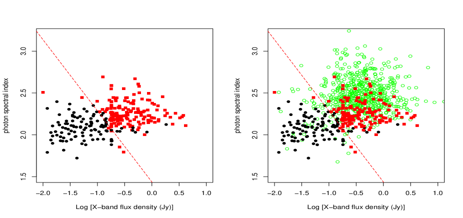
Figure 2: Classification scatterplots for the Fermi $\gamma$-ray photon spectral index ($\Gamma_{\rm ph}$) and the X-band VLBI radio flux (log$F_{R}$), where the black filled circles, red solid squares, and green empty circles indicate TBLs, FBLs and FSRQs respectively.

Table 2: The test accuracy, predict results , and parameters for the optimal combinations in RF algorithm.

N	$N_{\rm TBLLs}$	$N_{\rm FBLLs}$	Acc	p1	p2	p3	p4	p5	p6	p7	p8	p9	p10	p11	p12	p13
(1)	(2)	(3)	(4)	(5)	(6)	(7)	(8)	(9)	(10)	(11)	(12)	(13)	(14)	(15)	(16)	(17)
5∗	137	191	0.9889	2	4	5	7	13	…	…	…	…	…	…	…	…
6∗	138	190	0.9889	2	4	7	8	18	19	…	…	…	…	…	…	…
6	140	188	0.9889	2	4	5	7	13	18	…	…	…	…	…	…	…
6	141	187	0.9889	2	4	5	7	13	20	…	…	…	…	…	…	…
6	139	189	0.9889	2	4	5	12	13	19	…	…	…	…	…	…	…
6	140	188	0.9889	2	4	8	13	16	19	…	…	…	…	…	…	…
7∗	140	188	0.9889	2	4	5	7	9	13	18	…	…	…	…	…	…
7	141	187	0.9889	2	4	5	7	12	13	15	…	…	…	…	…	…
7	142	186	0.9889	2	4	5	7	12	13	19	…	…	…	…	…	…
7	143	185	0.9889	2	4	5	7	12	13	20	…	…	…	…	…	…
7	137	191	0.9889	2	4	5	7	13	15	17	…	…	…	…	…	…
7	138	190	0.9889	2	4	5	7	13	15	18	…	…	…	…	…	…
7	139	189	0.9889	2	4	5	7	13	15	19	…	…	…	…	…	…
7	142	186	0.9889	2	4	5	7	13	15	20	…	…	…	…	…	…
7	141	187	0.9889	2	4	5	7	13	16	18	…	…	…	…	…	…
7	143	185	0.9889	2	4	5	7	13	16	19	…	…	…	…	…	…
7	139	189	0.9889	2	4	5	7	13	20	22	…	…	…	…	…	…
7	128	200	0.9889	2	8	10	13	14	18	19	…	…	…	…	…	…
7	141	187	0.9889	2	4	8	13	14	19	21	…	…	…	…	…	…
7	138	190	0.9889	2	4	8	13	14	20	23	…	…	…	…	…	…
8∗	146	182	0.9889	2	4	7	8	13	18	19	20	…	…	…	…	…
8	142	186	0.9889	2	4	5	7	8	13	14	19	…	…	…	…	…
8	140	188	0.9889	2	4	5	7	9	12	13	19	…	…	…	…	…
8	137	191	0.9889	2	4	5	7	9	12	13	20	…	…	…	…	…
8	141	187	0.9889	2	4	5	7	9	13	18	23	…	…	…	…	…
8	141	187	0.9889	2	4	5	7	11	12	13	20	…	…	…	…	…
8	140	188	0.9889	2	4	5	7	11	13	16	22	…	…	…	…	…
8	143	185	0.9889	2	4	5	7	12	13	14	19	…	…	…	…	…
9∗	136	192	0.9889	2	4	6	8	12	13	14	19	20	…	…	…	…
9	136	192	0.9889	2	4	6	8	12	13	18	19	20	…	…	…	…
9	136	192	0.9889	2	4	7	10	13	14	18	19	20	…	…	…	…
9	134	194	0.9889	2	4	10	13	14	19	20	22	23	…	…	…	…
9	135	193	0.9889	2	4	5	7	8	10	13	20	21	…	…	…	…
9	133	195	0.9889	2	4	8	10	12	13	14	18	19	…	…	…	…
10∗	139	189	0.9889	2	4	5	7	8	12	13	15	19	22	…	…	…
11∗	136	192	0.9889	2	4	7	8	9	10	13	14	19	20	22	…	…
12∗	143	185	0.9889	2	4	5	7	12	13	15	18	19	20	21	22	…
13∗	144	184	0.9889	2	4	5	7	8	12	13	14	15	19	20	21	22
…	…	…	…	…	…	…	…	…	…	…	…	…	…	…	…	…

Note: The number of parameters for the optimal combination are presented in Column 1. The highest accuracies of each classifier are presented in Column 4. The number of true BL Lacs (TBLLs) and false BL Lacs (FBLLs) that possible intrinsically FSRQs predicted by Random Forests algorithm with the default settings for the LSP BL Lacs (predicted dataset) are presented in Columns 2 and 3. The labels of the parameters are presented in Columns 5-17, these correspond to the labels in Table 1, Column 1. Here, the one combination for the different number of parameters (e.g., $10^{*}$, $11^{*}$, $12^{*}$, and $13^{*}$) for the optimal combinations is shown for guidance regarding its form and content. (This table is available in its entirety in machine-readable form.)

Table 3: The Number of the Optimal Parameters and Combinations.

Algorithm	5Pars	6Pars	7Pars	8Pars	9Pars	10Pars	11Pars	12Pars	13Pars
RFs	1	5	14	35	52	39	28	2	2

Note: The Algorithm are presented in Column 1. The number of combinations with the highest accuracies in RFs algorithm for 5$-$13 parameters are presented in Columns 2$-$10 (see the machine-readable format of Table 2 for the details).

Table 4: The predicted classification results of Fermi LSP BL Lacs.

4FGL name	RF5	RF6	RF7	RF8	RF9	RF10	RF11	RF12	RF13	$C_{9}$	$M_{Fan}$	$M_{CKZ}$	CD	$M_{\rm wise}$
(1)	(2)	(3)	(4)	(5)	(6)	(7)	(8)	(9)	(10)	(11)	(12)	(13)	(14)	(15)
4FGL J0001.2$-$0747	fsrq	fsrq	fsrq	bll	bll	fsrq	fsrq	fsrq	bll	UNK	…	…	…	…
4FGL J0003.2$+$2207	bll	bll	bll	bll	bll	bll	fsrq	bll	bll	UNK	…	…	…	…
4FGL J0003.9$-$1149	fsrq	fsrq	fsrq	fsrq	fsrq	fsrq	fsrq	fsrq	fsrq	fsrq	…	…	…	…
4FGL J0006.3$-$0620	fsrq	fsrq	fsrq	fsrq	fsrq	fsrq	fsrq	fsrq	fsrq	fsrq	…	…	…	BZQ
4FGL J0008.0$+$4711	bll	bll	bll	bll	bll	bll	bll	bll	bll	bll	…	…	…	…
4FGL J0009.1$+$0628	bll	bll	bll	bll	bll	bll	bll	bll	bll	bll	…	…	…	…
4FGL J0013.1$-$3955	fsrq	fsrq	fsrq	fsrq	fsrq	fsrq	fsrq	fsrq	fsrq	fsrq	…	…	…	…
4FGL J0014.1$+$1910	fsrq	fsrq	fsrq	fsrq	fsrq	fsrq	fsrq	fsrq	fsrq	fsrq	…	…	1.41	…
4FGL J0019.6$+$2022	fsrq	fsrq	fsrq	fsrq	fsrq	fsrq	fsrq	fsrq	fsrq	fsrq	…	…	…	…
4FGL J0022.1$-$1854	bll	bll	bll	bll	bll	bll	bll	bll	bll	bll	…	…	…	…
4FGL J0022.5$+$0608	bll	fsrq	bll	fsrq	fsrq	fsrq	fsrq	bll	fsrq	UNK	…	…	…	…
4FGL J0023.9$+$1603	bll	bll	bll	bll	bll	bll	bll	bll	bll	bll	…	…	…	…
4FGL J0029.0$-$7044	fsrq	fsrq	fsrq	bll	bll	fsrq	fsrq	bll	fsrq	UNK	…	…	…	…
4FGL J0032.4$-$2849	bll	fsrq	bll	fsrq	fsrq	fsrq	bll	fsrq	fsrq	UNK	…	…	1.26	…
4FGL J0035.8$-$0837	bll	bll	bll	bll	bll	bll	bll	bll	bll	bll	…	…	…	…
4FGL J0038.1$+$0012	bll	bll	bll	bll	bll	bll	bll	bll	bll	bll	…	…	…	…
4FGL J0040.3$+$4050	bll	bll	bll	bll	bll	bll	bll	bll	bll	bll	…	…	…	…
4FGL J0049.7$+$0237	fsrq	fsrq	fsrq	fsrq	fsrq	fsrq	fsrq	fsrq	fsrq	fsrq	Fan_fsrq	…	…	…
4FGL J0056.8$+$1626	fsrq	fsrq	fsrq	fsrq	fsrq	fsrq	fsrq	fsrq	fsrq	fsrq	…	…	…	BZQ
4FGL J0058.0$-$3233	bll	bll	bll	bll	bll	bll	bll	bll	bll	bll	…	…	…	…
4FGL J0105.1$+$3929	fsrq	fsrq	fsrq	fsrq	fsrq	fsrq	fsrq	fsrq	fsrq	fsrq	…	…	1.95	…
4FGL J0107.4$+$0334	fsrq	fsrq	fsrq	fsrq	fsrq	fsrq	fsrq	fsrq	fsrq	fsrq	…	…	…	…
4FGL J0112.1$+$2245	bll	bll	bll	bll	bll	bll	bll	bll	bll	bll	…	…	…	…
4FGL J0113.7$+$0225	fsrq	fsrq	fsrq	fsrq	fsrq	fsrq	fsrq	fsrq	fsrq	fsrq	…	…	…	…
4FGL J0124.8$-$0625	fsrq	bll	fsrq	fsrq	fsrq	fsrq	fsrq	fsrq	fsrq	UNK	…	…	…	…
4FGL J0125.3$-$2548	fsrq	fsrq	fsrq	fsrq	fsrq	fsrq	fsrq	fsrq	fsrq	fsrq	…	…	…	…
4FGL J0127.2$-$0819	bll	bll	bll	bll	bll	bll	bll	bll	bll	bll	…	…	…	…
4FGL J0141.4$-$0928	fsrq	fsrq	fsrq	fsrq	fsrq	fsrq	fsrq	fsrq	fsrq	fsrq	Fan_fsrq	…	…	…
4FGL J0142.7$-$0543	bll	bll	bll	fsrq	fsrq	bll	fsrq	bll	bll	UNK	…	…	…	…
4FGL J0144.6$+$2705	fsrq	fsrq	fsrq	fsrq	fsrq	fsrq	fsrq	fsrq	fsrq	fsrq	…	…	…	…
4FGL J0148.6$+$0127	bll	bll	bll	bll	bll	bll	bll	bll	bll	bll	…	…	…	…
4FGL J0202.7$+$4204	fsrq	fsrq	fsrq	fsrq	fsrq	fsrq	fsrq	fsrq	fsrq	fsrq	…	…	…	…
4FGL J0203.6$+$7233	fsrq	fsrq	fsrq	fsrq	fsrq	fsrq	fsrq	fsrq	fsrq	fsrq	…	…	…	…
4FGL J0203.7$+$3042	fsrq	fsrq	fsrq	fsrq	fsrq	fsrq	fsrq	fsrq	fsrq	fsrq	…	…	2.34	…
4FGL J0208.3$-$6838	bll	bll	bll	bll	bll	bll	bll	bll	bll	bll	…	…	…	…
4FGL J0208.5$-$0046	fsrq	fsrq	fsrq	fsrq	fsrq	fsrq	fsrq	fsrq	fsrq	fsrq	…	…	…	BZQ
4FGL J0209.9$+$7229	fsrq	fsrq	fsrq	fsrq	fsrq	fsrq	fsrq	fsrq	fsrq	fsrq	…	CKZ_fsrq	2.24	…
4FGL J0217.2$+$0837	fsrq	fsrq	fsrq	fsrq	fsrq	fsrq	fsrq	fsrq	fsrq	fsrq	…	…	…	…
4FGL J0219.5$+$0724	bll	bll	bll	bll	bll	bll	bll	bll	bll	bll	…	…	…	…
4FGL J0224.0$-$7941	fsrq	fsrq	fsrq	fsrq	fsrq	fsrq	fsrq	fsrq	bll	UNK	…	…	…	…
4FGL J0231.2$-$5754	bll	bll	bll	bll	bll	bll	bll	bll	bll	bll	…	…	…	…
4FGL J0238.6$+$1637	fsrq	fsrq	fsrq	fsrq	fsrq	fsrq	fsrq	fsrq	fsrq	fsrq	Fan_fsrq	…	2.69	…
4FGL J0241.0$-$0505	bll	fsrq	bll	bll	fsrq	bll	bll	bll	bll	UNK	…	…	…	BZQ
4FGL J0243.4$+$7119	bll	bll	bll	bll	bll	bll	bll	bll	bll	bll	…	…	…	…
4FGL J0245.1$-$0257	bll	bll	bll	bll	bll	bll	bll	bll	bll	bll	…	…	…	…
4FGL J0255.8$+$0534	bll	bll	bll	bll	bll	bll	bll	bll	bll	bll	…	…	…	…
4FGL J0258.1$+$2030	bll	bll	bll	bll	bll	bll	bll	bll	bll	bll	…	…	…	…
4FGL J0301.0$-$1652	fsrq	fsrq	fsrq	fsrq	fsrq	fsrq	fsrq	fsrq	fsrq	fsrq	…	…	…	…
4FGL J0312.9$+$3614	bll	bll	bll	bll	bll	bll	bll	bll	bll	bll	…	…	…	…
4FGL J0314.3$-$5103	fsrq	bll	fsrq	bll	fsrq	bll	bll	fsrq	bll	UNK	…	…	…	…
4FGL J0316.2$+$0905	bll	bll	bll	bll	bll	bll	bll	bll	bll	bll	…	…	…	…
4FGL J0334.2$-$3725	bll	bll	bll	bll	bll	bll	bll	bll	bll	bll	…	…	…	…
4FGL J0334.2$-$4008	fsrq	fsrq	fsrq	fsrq	fsrq	fsrq	fsrq	fsrq	fsrq	fsrq	Fan_fsrq	…	1.78	…
4FGL J0340.5$-$2118	fsrq	fsrq	fsrq	fsrq	fsrq	fsrq	fsrq	fsrq	fsrq	fsrq	…	…	…	…
4FGL J0348.6$-$1609	fsrq	fsrq	fsrq	fsrq	fsrq	fsrq	fsrq	fsrq	fsrq	fsrq	…	…	…	…
4FGL J0354.7$+$8009	fsrq	fsrq	fsrq	fsrq	fsrq	fsrq	fsrq	fsrq	fsrq	fsrq	…	…	…	…
4FGL J0359.4$-$2616	fsrq	fsrq	fsrq	fsrq	fsrq	fsrq	fsrq	fsrq	fsrq	fsrq	…	CKZ_fsrq	…	BZQ
4FGL J0402.0$-$2616	bll	bll	bll	bll	bll	bll	bll	bll	bll	bll	…	…	…	…
4FGL J0403.5$-$2437	fsrq	fsrq	fsrq	fsrq	fsrq	fsrq	fsrq	fsrq	fsrq	fsrq	…	CKZ_fsrq	…	BZQ
4FGL J0407.5$+$0741	fsrq	fsrq	fsrq	fsrq	fsrq	fsrq	fsrq	fsrq	fsrq	fsrq	Fan_fsrq	CKZ_fsrq	2.69	…
4FGL J0422.3$+$1951	fsrq	fsrq	fsrq	bll	bll	bll	fsrq	bll	bll	UNK	…	…	…	…
4FGL J0424.7$+$0036	fsrq	fsrq	fsrq	fsrq	fsrq	fsrq	fsrq	fsrq	fsrq	fsrq	…	…	…	…
4FGL J0424.9$-$5331	fsrq	fsrq	fsrq	fsrq	fsrq	fsrq	fsrq	fsrq	fsrq	fsrq	…	…	…	…
4FGL J0428.6$-$3756	fsrq	bll	fsrq	bll	fsrq	fsrq	fsrq	fsrq	fsrq	UNK	Fan_fsrq	…	6.31	BZQ
4FGL J0433.6$+$2905	bll	bll	bll	bll	bll	bll	bll	bll	bll	bll	Fan_fsrq	…	12.59	…
4FGL J0438.9$-$4521	fsrq	fsrq	fsrq	fsrq	fsrq	fsrq	fsrq	fsrq	fsrq	fsrq	Fan_fsrq	CKZ_fsrq	2.51	BZQ
…	…	…	…	…	…	…	…	…	…	…	…	…	…	…

Note: The 4FGL names are listed in Column 1. The predicted classification results using RF algorithm for the different parameter combinations in the work are shown in columns 2-10. The combined classification results ($C_{9}$ predictions) is presented in Column 11. Column 12 and 13 list the predicted classification results ($M_{Fan}$) in Fan & Wu (2019) and ($M_{CKZ}$) in Cheng et al. (2022), respectively. The CD values reported in Paliya et al. (2021) are listed in Column 14. The BZQs of WIBRaLS2 catalog reported in D’Abrusco et al. (2019) are listed in Column 15. Table 4 is published in its entirety in the machine-readable format. A portion is shown here for guidance regarding its form and content.

For the finally sub-selected 23 parameters of 1680 sources, there are 8388607 different combinations. Then, the optimal parameters combinations (OPCs) are searched based on the training, validation and forecast samples using the random forests algorithms. The default settings for the random forests classification functions ($randomForest()$ in R code) are used to simplify the calculations. After the predictive models are generated and assessed; an effective predictive model is used to forecast whether a LSP BL Lac belongs to the possible intrinsically FRSQ or the actually BL Lac class based on its predictor variables. The main steps to accomplish this in the R platform are publicly available.

The prediction accuracies of the different parameter combinations in the random forests SML algorithms are computed. The highest prediction accuracies for different combinations of parameters in the random forests algorithms (represented with a red dotted line) are illustrated in Figure 1. As the number of parameters increases, the accuracy gradually reaches its maximum. Here, with 5, 6, 7, 8, 9, 10, 11, 12, or 13 parameters combinations (see Table 2), the accuracy of the random forests algorithm reaches its maximum. Where, 178 OPCs in total 8388607 different combinations are hunted. There is 1, 5, 14, 35, 52, 39, 28, 2, or 2 combinations of 5, 6, 7, 8, 9, 10, 11, 12, or 13 parameters achieving a maximum accuracy (accuracy $\simeq$ 0.9889) respectively (see Table 2 and 3). When more parameters are applied, the accuracy begins to decline, which are consistent with the conclusions of our previous work (Kang et al. 2019b).

From the 178 OPCs (see Table 2 and 3), we select nine combinations, one combination in one of the combinations with 5, 6, 7, 8, 9, 10, 11, 12, or 13 parameters, respectively (see Table 2 for the parameter with underline and marked ^∗ in the number of parameters, e.g., 5^∗). Combined the classification results from the nine OPCs ($C_{9}$ predictions), 113 true BL Lacs (TBLs) and 157 false BL Lacs (FBLs) that possible intrinsically FSRQs misclassified as BL Lacs, are predicted, where 58 remain without a clear prediction, for 328 LSP BL Lacs reported in the high Galactic latitudes ($|b|>10\deg$) 4LAC-DR2 catalog. The predicted results of 328 LSP BL Lacs are listed in Table 4.

In the $\Gamma_{\rm ph}$-${\rm log}{F_{R}}$ (Fermi $\gamma$-ray photon spectral index and the X-band VLBI radio flux) plane for the LSP BL Lacs, we note that the prediction results, between the 113 TBLs (black dots) and 157 FBLs (red squares), show a clear separation (see Figure 2). In the two-dimensional parameters space, a simply phenomenological critical line (e.g., $A{\times}x+B{\times}y+C=0$) can be employed to roughly separate these two subclasses (TBLs and FBLs) (e.g., see Chen 2018; Xiao et al. 2022a). Which (this criterion/line) can be obtained from the Support Vector Machines (SVM, the function $svm()$ of the e1071 package in R, see Meyer et al. 2021 for details) with kernel = “linear” (other settings with default) in two-dimensional parameters space. The optimal critical lines (e.g., see equation 3 identified as the dotted-dashed red lines in Figure 2) with the accuracy value: 92.86% are obtained in the $\Gamma_{\rm ph}$-${\rm log}{F_{R}}$ plane:

$$3.85\times\Gamma_{\rm ph}+3.27\times{\rm log}{F_{R}}-5.54=0.$$ (3)

Of these, 96 of the 113 TBLs (96/113$\simeq$84.96%) are in the lower left of the line; 151 of the 157 FBLs (151/157$\simeq$96.18%) are in the upper right of the line.

Table 5: The median and mean of ${\rm log}{F_{R}}$ and $\Gamma_{\rm ph}$ for TBLs, FBLs, FSRQs

	TBLs			FBLs			FSRQ
Paras	mean	median		mean	median		mean	median
(1)	(2)	(3)		(4)	(5)		(6)	(7)
${\rm log}{F_{R}}$	-1.259	-1.232		-0.434	-0.381		-0.414	-0.404
$\Gamma_{\rm ph}$	2.089	2.092		2.265	2.244		2.472	2.450

Note: Column 1 presents the parameters. Column 2 and 3 list the mean and median of TBLs; Column 4 and 5 list the mean and median of FBLs; Column 6 and 7 list the mean and median of FSRQs, respectively.

Table 6: Comparison of the other work’s Predictions.

Algorithm	Class	RF Predictions	Fan Predictions	CKZ Predictions	CKZ Predictions	Paliya Predictions	WIBRaLS2
	N	328	33 FSRQs	47 FSRQs	39 FSRQs	626 CD $>$ 1	5089 BZQs
	M	328	29	39	31	33	37
	FSRQ	157	24	38	30	22	33
RF	BLL	113	2	…	…	5	1
	UNK	58	3	1	1	6	3

Note: The classifiers and classes are presented in Column 1 and 2. Columns 3 lists the results of random forests Predictions in the work. Columns 4-7 presents the results of comparison of the Fan’s predictions in Fan & Wu (2019); the CKZ’s predictions in Cheng et al. (2022) (where, Columns 6 lists the sources have CD) ; the Paliya’s Predictions in Paliya et al. (2021); the WIBRaLS2’s results in D’Abrusco et al. (2019) for common objects. Where, N is the number of the Fan’s predictions, CKZ’s predictions, Paliya’s Predictions, and WIBRaLS2’s results; M shows the number of random forests Predictions of the work in the cross-matching the FAN’s predictions, CKZ’s predictions, Paliya’s Predictions, and WIBRaLS2’s results.

Comparing the FBLs with the TBLs and the FSRQs reported in 4LAC (green open squares in right panel in Figure 2), we found that the ${\rm log}{F_{R}}$ with a median of -0.381 (or a mean of -0.434) and $\Gamma_{\rm ph}$ with a median of 2.244 (or a mean of 2.265) of the FBLs are both slightly larger than that of the TBLs with a median of -1.232 (or a mean of -1.259) and a median of 2.092 (or a mean of 2.089) respectively (see Table 5). The ${\rm log}{F_{R}}$ of the FBLs with a median of -0.381 (or a mean of -0.434) and that of the FSRQs with a median of -0.404 (or a mean of -0.414) are overlapping and cannot be distinguished; However, the photon spectral index of FBLs with a median of 2.244 (or a mean of 2.265) is slightly smaller than that of FSRQs with a median of 2.450 (or a mean of 2.472). The FBLs are located in a regions where the ${\rm log}{F_{R}}$ is large relative to the TBLs and the the photon spectral index is small relative to the FSRQs. These FBLs may be intrinsically FSRQs with broad emission lines, which were mistaken for BL Lac-type sources due to their strong jet continuum swamping the broad emission lines and showing relatively small EW. When the continuum becomes weaker, the emission lines should exhibit a larger FSRQ-type EWs. The FBLs are the candidates for the transition from BL Lac to FSRQ (B-to-F transition), and the region (above line), where the FBLs are located in (see Figure 2), can be referred to as the from BL Lac to FSRQ transition region, called as B-to-F transition region (named as “$B\rightarrow{F}$ zone”).

5 Results comparison

5.1 Comparison with the predictions

Cross-matching the $C_{9}$ predictions (FBLs) and the predictions of Fan & Wu (2019), of the 33 LSP BL Lac sources predicted as the possible FSRQ type sources by Fan & Wu (2019), there are 29 sources in our sample. Among the 29 possible FSRQ type sources predicted by Fan & Wu (2019), the prediction results of 24 (24/29 $\simeq$ 82.76%) sources in the work are consistent with the results of Fan & Wu (2019); However, 3 sources (4FGL J0428.6-3756; 4FGL J0811.4+0146 and 4FGL J0818.2+4222) are still no clear predictions; and 2 sources (4FGL J0433.6+2905 and 4FGL J0738.1+1742) are predicted as true BL Lacs in our work (see Table 4 and 6).

In Paliya et al. (2021), the Compton dominance (CD; the ratio of the inverse Compton to synchrotron peak luminosities) for 1030 Fermi blazars are calculated. They found that the CD and accretion luminosity ($L_{\rm disk}$) in Eddington units ($L_{\rm disk}/L_{\rm Edd}$) are positively correlated, suggesting that the CD can be used to reveal the state of accretion in blazars and used to distinguish the classification of blazars. They suggest that blazars with CD $>$ 1 should be identified as FSRQs and CD $<$ 1 as BL Lac objects. There are 626 blazars with CD $>$ 1 in their sample. Cross-matching the $C_{9}$ prediction results and the 626 blazars identified as FSRQs in Paliya et al. (2021), we obtained 33 common sources. Among the 33 common objects, 22 (22/33 $\simeq$ 66.67%) FSRQ candidates are consistent between our predictions and Paliya et al. (2021) predictions (see Table 4 and Table 6). 5 TBLs (4FGL J0433.6+2905; 4FGL J1008.8-3139; 4FGL J1035.6+4409; 4FGL J1503.5+4759 and 4FGL J1942.8-3512) and 6 UNKs (4FGL J0032.4-2849 ; 4FGL J0428.6-3756; 4FGL J0811.4+0146; 4FGL J1331.2-1325; 4FGL J1647.5+4950 and 4FGL J1704.2+1234) were predicted in our work.

The WIBRaLS2 catalog (D’Abrusco et al., 2019) includes 9541 sources that is an incremental version of the WISE Blazar-like Radio-Loud Sources (WIBRaLS) catalog (D’Abrusco et al. 2014). Based on their WISE colors, these sources are classified as 3744 BL Lacs, 5089 flat-spectrum radio quasars (BZQs), and 708 mixed candidates. Cross-matching the $C_{9}$ predictions and the 5089 BZQs in D’Abrusco et al. (2019), there are 37 BZQs in our prediction sample. Among the 37 BZQs, the prediction results of 33 (33/37 $\simeq$ 89.19%) sources in this work are consistent with the results of D’Abrusco et al. (2019); However, 3 sources (4FGL J0241.0-0505; 4FGL J0428.6-3756; and 4FGL J0818.2+4222) are still no clear predictions; and 1 sources (4FGL J1135.1+3014) are predicted as true BL Lacs in this work (see Table 4 and 6).

When cross-matching the $C_{9}$ predictions and the prediction results of Cheng et al. (2022), 39 of the 47 LSP BL Lac sources predicted as FSRQ are in our sample. The remaining 8 sources locate in the low Galactic latitudes ($|b|<10\deg$) 4LAC-DR2 catalog. Among the 39 sources, the prediction results of 38 sources (38/39 $\simeq$ 97.44%) are consistent with our prediction results. There is only one source (4FGL J2241.2+4120) that does not have a clear prediction in the work (see Table 4 and Table 6). In Cheng et al. (2022), they also check the CD of 39 sources based on SEDs fitting using a quadratic polynomial. For the 39 sources (see Columns 6 in Table 6) reported the CD in Cheng et al. (2022), 31 sources are in our sample, the other remaining 8 sources locate in the low Galactic latitudes ($|b|<10\deg$) 4LAC-DR2 catalog. There are 30 (30/31 $\simeq$ 96.77%) sources’ prediction are consistent with our predictions, in which 28 sources with CD $>$ 1; two sources with CD $<$ 1; One source (4FGL J2241.2+4120 with CD $\simeq$ 3.689) that does not have a clear prediction in our work; As mentioned above, a comparison (the prediction results of approximately exceeding (24+38+30+22+33)/(29+39+31+33+37) $\simeq$ 86.98% are consistent) of these predictions suggests that our predictions may be promising.

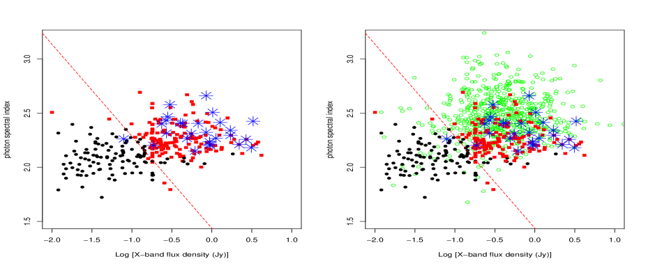
Figure 3: Classification scatterplots for the Fermi $\gamma$-ray photon spectral index ($\Gamma_{\rm ph}$) and the X-band VLBI radio flux (log $F_{R}$), where the black filled circles, red solid squares, and green empty circles indicate TBLs, FBLs and FSRQ respectively. And the blue stars represent the LSP Changing-Look Blazars reported in Foschini et al. 2022, 2021.

5.2 Comparison with the CLBs

Table 7: The LSP CLBs reported in Foschini et al. 2022.

N	4FGL name	Optical class	SED class	$\Gamma_{\rm ph}$	log$F_{R}$
1	4FGL J0407.5$+$0741	bll	LSP	2.311	-0.257
2	4FGL J1302.8$+$5748	bll	LSP	2.267	-0.310
3	4FGL J1751.5$+$0938	bll	LSP	2.258	0.428
4	4FGL J1800.6$+$7828	bll	LSP	2.210	0.343
5	4FGL J2134.2$-$0154	bll	LSP	2.295	0.233
6	4FGL J0217.8$+$0144	fsrq	LSP	2.236	-0.029
7	4FGL J0449.1$+$1121	fsrq	LSP	2.507	0.011
8	4FGL J0509.4$+$1012	fsrq	LSP	2.408	-0.395
9	4FGL J0510.0$+$1800	fsrq	LSP	2.200	-0.021
10	4FGL J0719.3$+$3307	fsrq	LSP	2.203	-0.733
11	4FGL J0833.9$+$4223	fsrq	LSP	2.434	-0.572
12	4FGL J1037.4$-$2933	fsrq	LSP	2.414	0.104
13	4FGL J1043.2$+$2408	fsrq	LSP	2.323	-0.072
14	4FGL J1124.0$+$2336	fsrq	LSP	2.406	-0.365
15	4FGL J1224.9$+$2122	fsrq	LSP	2.342	0.232
16	4FGL J1322.2$+$0842	fsrq	LSP	2.262	-1.102
17	4FGL J1333.2$+$2725	fsrq	LSP	2.315	-0.567
18	4FGL J1422.3$+$3223	fsrq	LSP	2.401	-0.627
19	4FGL J1657.7$+$4808	fsrq	LSP	2.406	-0.171
20	4FGL J1937.2$-$3958	fsrq	LSP	2.661	-0.072
21	4FGL J2026.0$-$2845	fsrq	LSP	2.578	-0.523
22	4FGL J2158.1$-$1501	fsrq	LSP	2.181	0.495
23	4FGL J2212.0$+$2356	fsrq	LSP	2.212	-0.024
24	4FGL J2225.7$-$0457	fsrq	LSP	2.425	0.517
25	4FGL J2236.3$+$2828	fsrq	LSP	2.268	0.051
26	4FGL J2345.2$-$1555	fsrq	LSP	2.150	-0.211
27	4FGL J2349.4$+$0534	fsrq	LSP	2.467	-0.551

Note: The number of the records are presented in Column 1. Column 2 lists the source name of 4FGL. The optical classes and the SED class reported in 4FGL are presented in Column 3 and Column 4, respectively, where “bll” indicates BL Lac and “fsrq” indicates FSRQ. A simple horizontal line is used to distinguish the FSRQs and BL lacs. The $\gamma$-ray photon spectral index ($\Gamma_{\rm ph}$) and the X-band VLBI radio flux (log$F_{R}$) are shown in Columns 5 and 6; respectively.

In Ajello et al. (2020), they found that the $\nu^{\rm S}_{\rm p}$ distributions are overlap between LSP BL Lacs and FSRQs, and the gamma-ray photon spectral index ($\Gamma_{\rm ph}$) distributions are also very similar. They proposed that there is a possible region for objects that might be transitioning between FSRQs and BL Lacs. There are five of six such transitioning objects found by Ruan et al. (2014) are the LSP subclass reported in 4LAC. In addition, Pei et al. (2022) also address a similar area, based on disk luminosity ($L_{\rm disk}$) in Eddington units ($L_{\rm disk}/L_{\rm Edd}$). They proposed that there is a region (called “appareling zone”) with $2.00\times 10^{-4}~{}\lesssim~{}L_{\rm disk}/L_{\rm Edd}~{}{\lesssim}~{}8.51\times 10^{-3}$, where, some sources (that are perhaps changing-look blazars) may be a transition between BL Lacs and FSRQs. And they found five confirmed changing-look sources reside in the “appareling zone”.

In the work, a B-to-F transition zone (transition from BL Lac to FSRQ) is suggested by comparing the prediction results: TBLs and FBLs. In order to test the effectiveness of the B-to-F zone. Where, whether some LSP BL Lacs (e.g., FBLs) are located in the “$B\rightarrow{F}$ zone” that are the most likely Candidates of Changing-Look Blazar. We check a LSP CLBs sample that was collected by Foschini et al. (2022, 2021). All of which are compiled into an online (Transition) Changing-Look Blazars Catalog (TCLB Catalog, https://github.com/ksj7924/CLBCat) (Kang et al., in preparation) presented in https://github.com/ for easy communication. In Foschini et al. (2022, 2021), they compiled a gamma-ray jetted AGN sample based on the 4FGL catalog. They reported 34 Changing-Look AGNs, 32 of them are labeled as blazars (24 FSRQs, 7 BL Lacs, and 1 BCU) in 4FGL catalog, based on a significant change in optical spectral lines (disappearance and reappearance) in different observation epochs reported in the previous literature (see Foschini et al. 2022, 2021 for more details and references therein). Among the them, there are 27 LSP CLBs (22 LSP FSRQ type and 5 LSP BL Lac type) in our sample and which are listed in Table 7. A simple horizontal line is used to distinguish the LSP FSRQs and LSP BL lacs labeled in 4FGL.

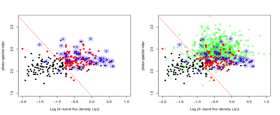
Figure 4: Classification scatterplots for the Fermi $\gamma$-ray photon spectral index ($\Gamma_{\rm ph}$) and the X-band VLBI radio flux (log $F_{X}$), where the black filled circles, red solid squares, and green empty circles indicate TBLs, FBLs and FSRQs respectively. And the blue stars represent the LSP BL Lac type Changing-Look Blazars reported in Xiao et al. (2022a).

For ease of comparison, the classification scatterplots for the Fermi $\gamma$-ray photon spectral index ($\Gamma_{\rm ph}$) and the X-band VLBI radio flux (log$F_{R}$) are plotted in Figure 3, where the black filled circles, red solid squares, and green empty circles indicate TBLs, FBLs predicted in this work and FSRQs labeled in 4FGL, respectively. And the blue stars represent the LSP CLBs (22 LSP FSRQ type and 5 LSP BL Lac type sources) are reported in Foschini et al. 2022, 2021. The left panels represent the correlation between $\Gamma_{\rm ph}$ and log$F_{\rm R}$ of the TBLs and FBLs predicted in this work and CLBs identified in Foschini et al. 2022, 2021. In the right panels, the FSRQs labeled in 4FGL are also added (see, green circle).

In Figure 3, for the entire LSP CLBs, we note that most of the LSP CLBs (26 of 27 sources, $\simeq$ 96.29%) are located in the B-to-F transition zone. Only one source, 4FGL J1322.2+0842 with $\Gamma_{\rm ph}=2.262$, and log$F_{R}=-1.102$ labeled as LSP FSRQ in 4FGL catalog, that do not locate in the B-to-F transition zone. Where, there are 21 FSRQ type CLBs, which is that the LSP BL Lacs that may have transitioned from BL Lacs to FSRQs. The results suggest the B-to-F transition region is valid for LSP BL Lac. Where some LSP BL Lacs (e.g., FBLs) are located in the “$B\rightarrow{F}$ zone” that are the most likely Candidates of Changing-Look Blazars.

In addition, recently, in Xiao et al. (2022b), they reported 52 new Changing-look blazars (10 FSRQs and 42 BL Lacs) based on the EW classification of their optical spectra. There are 45 LSP CLBs in our sample and are listed in Table 8, which includes 10 LSP FSRQ type CLBs and 35 LSP BL Lac type CLBs. A simple horizontal line is used to distinguish the FSRQs and BL lacs. All the 35 LSP BL Lacs that are in our forecast sample. Among the 35 LSP BL Lacs, the prediction results of 29 (29/35 $\simeq$ 82.86%) sources are consistent with our prediction results; 3 TBLs (4FGL J0433.6$+$2905, 4FGL J0654.7$+$4246, and 4FGL J1503.5$+$4759) and 3 UNKs (4FGL J0428.6$-$3756, 4FGL J1331.2$-$1325, 4FGL J1647.5$+$4950) were predicted in our work.

In Figure 4, these CLBs reported in Xiao et al. (2022b) also were plotted. For the 10 LSP FSRQ type CLBs, that are all located in the B-to-F transition region. For the 35 LSP BL Lac type CLBs (see Table 8), we note that except for one source (4FGL J1058.0+4305) without radio data (see Table 8); three source (4FGL J0654.7+4246 and 4FGL J1503.5+4759 are evaluated as TBLs, and 4FGL J1331.2-1325 is evaluated as UNKs) is not located in the B-to-F transition region; 31 of them are all located in the B-to-F transition region. For the entire 45 LSP CLBs, there are 41 (41/45 $\simeq$ 91.11%) LSP CLBs (31 BL Lacs and 10 FSRQs) are located in the B-to-F transition region. These results also further indicate that the B-to-F transition region is valid for the LSP BL Lac subclass. Where some LSP BL Lacs (e.g., FBLs) are located in the “$B\rightarrow{F}$ zone” that are the most likely Candidates of Changing-Look Blazars.

Table 8: The Changing-Look blazars reported in Xiao et al. 2022a.

N	4FGL name	Optical class	SED class	$\Gamma_{\rm ph}$	log$F_{R}$
1	4FGL J0006.3$-$0620	bll	LSP	2.128	0.397
2	4FGL J0203.7$+$3042	bll	LSP	2.239	-0.638
3	4FGL J0209.9$+$7229	bll	LSP	2.275	-0.389
4	4FGL J0238.6$+$1637	bll	LSP	2.165	0.127
5	4FGL J0334.2$-$4008	bll	LSP	2.183	0.131
6	4FGL J0407.5$+$0741	bll	LSP	2.311	-0.257
7	4FGL J0428.6$-$3756	bll	LSP	2.098	-0.283
8	4FGL J0433.6$+$2905	bll	LSP	2.078	-0.556
9	4FGL J0438.9$-$4521	bll	LSP	2.417	-0.077
10	4FGL J0516.7$-$6207	bll	LSP	2.176	-0.069
11	4FGL J0538.8$-$4405	bll	LSP	2.111	0.597
12	4FGL J0629.3$-$1959	bll	LSP	2.231	-0.012
13	4FGL J0654.7$+$4246	bll	LSP	2.006	-0.939
14	4FGL J0710.9$+$4733	bll	LSP	2.670	-0.306
15	4FGL J0831.8$+$0429	bll	LSP	2.273	-0.162
16	4FGL J0832.4$+$4912	bll	LSP	2.378	-0.384
17	4FGL J1001.1$+$2911	bll	LSP	2.269	-0.462
18	4FGL J1058.0$+$4305	bll	LSP	2.346	…
19	4FGL J1058.4$+$0133	bll	LSP	2.233	0.581
20	4FGL J1058.6$-$8003	bll	LSP	2.258	0.280
21	4FGL J1147.0$-$3812	bll	LSP	2.229	0.247
22	4FGL J1250.6$+$0217	bll	LSP	2.057	-0.406
23	4FGL J1331.2$-$1325	bll	LSP	2.600	-1.509
24	4FGL J1503.5$+$4759	bll	LSP	2.221	-1.319
25	4FGL J1647.5$+$4950	bll	LSP	2.386	-0.893
26	4FGL J1751.5$+$0938	bll	LSP	2.258	0.428
27	4FGL J1800.6$+$7828	bll	LSP	2.210	0.343
28	4FGL J1806.8$+$6949	bll	LSP	2.297	0.096
29	4FGL J1954.6$-$1122	bll	LSP	2.443	-0.479
30	4FGL J2134.2$-$0154	bll	LSP	2.295	0.233
31	4FGL J2152.5$+$1737	bll	LSP	2.270	-0.284
32	4FGL J2202.7$+$4216	bll	LSP	2.202	0.515
33	4FGL J2216.9$+$2421	bll	LSP	2.284	-0.140
34	4FGL J2315.6$-$5018	bll	LSP	2.395	-0.434
35	4FGL J2357.4$-$0152	bll	LSP	2.315	-0.747
36	4FGL J0102.8$+$5824	fsrq	LSP	2.292	0.335
37	4FGL J0337.8$-$1157	fsrq	LSP	2.724	-0.833
38	4FGL J0347.0$+$4844	fsrq	LSP	2.577	-0.883
39	4FGL J0521.3$-$1734	fsrq	LSP	2.374	-0.717
40	4FGL J0539.6$+$1432	fsrq	LSP	2.545	-0.431
41	4FGL J0539.9$-$2839	fsrq	LSP	2.731	-0.037
42	4FGL J0601.1$-$7035	fsrq	LSP	2.418	-0.389
43	4FGL J1816.9$-$4942	fsrq	LSP	2.391	-0.783
44	4FGL J2015.5$+$3710	fsrq	LSP	2.453	0.418
45	4FGL J2121.0$+$1901	fsrq	LSP	2.220	-0.706

Note: The number of the records are presented in Column 1. Column 2 lists the source name of 4FGL. The optical classes and the SED class reported in 4FGL are presented in Column 3 and Column 4, respectively, where “bll” indicates BL Lac and “fsrq” indicates FSRQ. A simple horizontal line is used to distinguish the FSRQs and BL lacs. The $\gamma$-ray photon spectral index ($\Gamma_{\rm ph}$) and the X-band VLBI radio flux (log$F_{R}$) are shown in Columns 5 and 6; respectively.

6 Discussion and Conclusion

A portion of BL Lacs, which showed the observational characteristics of FSRQ type sources, could be potential FSRQs, vice versa. The peculiar rare transition phenomenon that have found between BL Lacs and FSRQs (e.g., EW become larger or smaller) has been addressed by some authors. Which is common addressed by some possible scenarios in the previous literature (e.g., see Peña-Herazo et al. 2021 for the related discussions and references therein). For instance, the broad lines (EW) of some transition sources may be swamped by the strong (beamed) jet continuum variability (e.g., Vermeulen et al. 1995; Giommi et al. 2012; Ruan et al. 2014; Pasham & Wevers 2019), or jet bulk Lorentz factor variability (e.g., Bianchin et al. 2009); Or some transition sources with weak radiative cooling, the broad lines are overwhelmed by the non-thermal continuum (e.g., Ghisellini et al. 2012). In addition, some strong broad lines of the FSRQ type source are missed due to with a high redshift (e.g., $z>0.7$, D’Elia et al. 2015), the one of the strongest $H{\alpha}$ line falls outside the optical window, caused the misclassification. Also, several observational effects (e.g., signal-to- noise ratio, and spectral resolution, etc.) may also affected the optical classification (see Peña-Herazo et al. 2021 for the related discussions). In-depth research is of great significance to deepen the understanding of the origin of transition (e.g., CLB type) sources, the accretion state transition of supermassive black holes; jet particle acceleration process; and black hole-galaxy co-evolution, etc (e.g., Ruan et al. 2014; Mishra 2021).

Based on the 4LAC, 4FGL and RCF catalog, we constructed a sample containing 1680 Fermi sources with known EW-based (optical) classifications (FSRQs and BL Lacs) and SED-based classifications (LSP, ISP, and HSP). Which includes 651 FSRQs and 1029 BL Lacs, that are divided into 960 LSP, 334 ISP and 386 HSP sources. Where, 1352 blazars with 651 FSRQs and 701 ISP and HSP BL Lacs are viewed as the training and validation samples; All 328 LSP BL Lacs are viewed as a forecast sample. Approximately 4/5 of 1352 blazars are randomly (random seed = 123) assigned to the training sample, and the remaining ones (e.g., approximately 1/5) are considered as the validation sample. Here, the training sample include 1082 blazars with 528 FSRQs and 554 HSP (and LSP) BL Lacs, and the validation sample has 270 blazars with 123 FSRQs and 147 ISP, or HSP BL Lacs. Based on the D $>$ 0.3 in the two sample K-S test and Gini $>$ 2.1 in random forests algorithm for all parameters with valid observations, there are 23 parameters selected in the work for the 1680 sources. Using the the random forests algorithm with the default settings for the random forests classification functions ($randomForest()$ in R code) to the selected sample (the training, validation and forecast samples), the 8388607 different combinations for the selected 23 parameters are calculated. There are 178 OPCs (the optimal parameters combinations) with a maximum accuracy (accuracy$\simeq$0.9889) are obtained, where, 1, 5, 14, 35, 52, 39, 28, 2, or 2 combinations of 5, 6, 7, 8, 9, 10, 11, 12, or 13 parameters (see Table 3), respectively. We select nine combinations, one combination in the combinations with 5, 6, 7, 8, 9, 10, 11, 12, or 13 parameters, respectively. Combined the classification results from the nine optimal combinations of parameters, 113 TBLs and 157 possible FBLs are predicted; however, 58 remain without a clear prediction; for 328 LSP BL Lacs reported in the high Galactic latitudes ($|b|>10\deg$) 4LAC-DR2 catalog.

In section 5, the prediction results between our ($C_{9}$) predictions of this work using random forests algorithm and the Fan’s predictions (Fan & Wu, 2019), CKZ’s predictions (Cheng et al., 2022), Paliya’s Predictions (Paliya et al., 2021), or WIBRaLS2 catalog’s results (D’Abrusco et al., 2019) are compared, respectively. Among the common objects through cross-matching, the prediction results of most of the sources are consistent (see Table 6). It suggests that our predictions are robust and effective. However, we should note that among the 1680 selected sample sources, there are 167 source X-band flux data missing in the training and validation sample and 30 source X-band flux data missing in the forecast sample. In the random forests algorithm, the missing data is filled with the median using the $na.roughfix()$ function of the random forests algorithm. Based on a set of combined parameters, we test that the predictions of missing data with mean filling are basically consistent with that of with the median filling; We also tested, delete the source of missing data, the prediction results are basically the same. However, the prediction accuracy decreased slightly (accuracy $\simeq$0.9728), which basically had no effect on our main conclusions. Also, there are a total of 178 optimal parameters combinations (OPC) with a maximum accuracy and we select only 9 of these OPCs to combine and construct our prediction results ($C_{9}$ predictions, see Table 2 and 4). We also tried crossing more parameter combinations, the predictions FBLs and TBLs had slightly fewer sources, and UNK sources had slightly more sources. From various combinations, we select only a part of them, which have a little effect on the final prediction result. In addition, some sources without SED classes were removed, possibly with selection effects. In the random forest calculation, the $randomForest()$ function using the default setting, and the random factor is set as: seed=123, also slightly affect the forecast results (see Kang et al. 2019a for some related discussion), also need to note.

Moreover, we also should note that the misclassified BL Lacs are singled out only from the LSP BL Lacs and only based the observational properties: 22 Fermi-specific parameters plus a radio flux from the RFC in the work. For the ISP/HSP BL Lacs as possible FBLs that should have relatively high powers and peak frequency ($\nu^{\rm S}_{\rm p}$) values of the synchrotron bump (e.g., Georganopoulos & Marscher 1998; Giommi et al. 2012; Kaur et al. 2017; Padovani et al. 2019 and references therein) and other parameters (e.g., Eddington ratios, equivalent to the accretion rates and powers, etc), which are not considered (dismissed) in the work, may be further addressed in future work.

In addition, we also should note that the analysis in this work is purely based in gamma-rays and radio-frequencies data and the sources were evaluated using a random forest algorithm. We only evaluated that some BL Lacs showed the observational characteristics of FSRQ type sources could be potential FSRQs. However, for their true classifications, an optical spectroscopic follow up would be needed to prove it. We should know that blazars usually display large amplitude and rapid variability across the electromagnetic spectrum. The EW value measured from optical spectra is common based on a single-epoch classification. Which may be affected by the variability of blazars. For instance, the broad lines (EW) may be swamped by the strong (beamed) jet continuum variability (e.g., Vermeulen et al. 1995; Giommi et al. 2012; Ruan et al. 2014; Pasham & Wevers 2019). However, the 4FGL catalog is based on 10 years of observations of Fermi-LAT data and its parameter’s values are calculated from central tendency values. Which may be less affected by the variability of blazars and more reflective of its intrinsic characteristics than the value of EW. Therefore, the issues in the context may be more reasonable. We expect further research to verify whether the hypothesis is reasonable or not. However, its essential classification still needs to be confirmed by optical spectra.

Comparing the predictions: between TBLs and FBLs, we find that the FBLs show a clear separation for TBLs in the $\Gamma_{\rm ph}$-${\rm log}{F_{R}}$ plane, which can use a simple phenomenological critical line (see Equation 3 and Figure 2) to roughly separate these two subclasses, where, the FBLs are located in higher areas. Checking the LSP CLBs, there are 26 of 27 LSP CLBs are located in the transition zone. Therefore, we propose a B-to-F transition zone named “$B\rightarrow{F}$ zone” where the transition from BL Lac to FSRQ will occur for LSP BL Lac. Where, some LSP BL Lacs (e.g., FBLs) are located in the “B → F zone” that are the most likely Candidates of Changing-Look Blazar.

We note that the EW of the changing-look blazar B2 1420+32 is close to 5Å, and floats around 5Å, sometimes the EW is greater than 5Å, sometimes less than 5Å, during between FSRQ and BL Lac state transitions (Mishra et al., 2021). For the FBLs that are the possible Candidates of Changing-Look Blazar found in the work, whether the EWs of them are also close to 5Å, we will do further verification next.

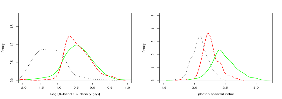
Figure 5: the density distribution for the photon spectral index ($\Gamma_{\rm ph}$, right panel) and the X-band flux (log $F_{R}$, left panel), where the black dashed lines, red long-dashed lines, and green solid lines indicate TBLs, FBLs , and FSRQs respectively.

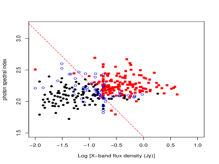
Figure 6: Scatterplots for the photon spectral index ($\Gamma_{\rm ph}$) and the X-band flux (log $F_{R}$), where the black filled circles, red solid squares, and blue empty circles indicate TBLs, FBLs and UNKs respectively.

Moreover, we should note that we only address the transition from LSP BL Lacs to FSRQs in the work and only suggest a “$B\rightarrow{F}$ zone”. Using the B-to-F transition zone, the LSP FBLs can be well identified from LSP BL Lacs. We also note that all the LSP BL Lac type CLBs are located in the B-to-F transition region (see Figure 3 in Section 5). Almost all the LSP FSRQ type CLBs are located in the B-to-F transition region, only one source (4FGL J1322.2$+$0842 with $\Gamma_{\rm ph}$ = 2.262 and ${\rm log}{F_{R}}$ = -1.102) are not in. But, the source is very close to the critical line. Which imply that these LSP FSRQ type CLBs may be some LSP BL Lacs that have transitioned, may be BL Lacs before the transition (e.g., see Foschini et al. 2021, 2022, some FSRQs, featureless or weaker lines in previous literature). This also further indicates that the B-to-F transition zone can effectively screen out those potential FBLs (e.g., Changing-Look type blazars) from LSP BL Lacs, which verifies the validity/effectiveness of the B-to-F transition zone. In addition, vice versa, a transition from FSRQs to BL Lacs (F-to-B transition) is also possible. The possible candidates for the F-to-B transition that cannot be addressed only based on this work. Which needs to be further addressed in the future. When the F-to-B transition candidate sources are also screened, the F-to-B transition region can be effectively demarcated. Also, the complete CLBs (B$\rightleftarrows$F) transition region (B-to-F transition, Vice versa) may be proposed. And the role of CLB in the blazar sequence, its evolution (e.g., blazar redshift evolution), origin and other issues can be further discussed/studied (Ruan et al. 2014). Also, the “$B\rightarrow F$ zone” is obtained only based on the two parameters of the ${\rm log}{F_{R}}$ and $\Gamma_{\rm ph}$. We also tried to check all possible combinations of the 23 parameters, but there was no other better findings. For other parameters (or multi-dimensional parameter space) whether there are similar regions, or better discrimination, further research is needed.

In addition, we also should note that the density distribution of the $\Gamma_{\rm ph}$ (right panel in Figure 5) and the log $F_{R}$ (left panel) for the TBLs, FBLs, and FSRQs show a different distributions. The ${\rm log}{F_{R}}$ of the TBLs and that of the FSRQ are clearly distinguished, where the D = 0.858 and p $<$ 1E-16 for the two-sample K-S test, however, the ${\rm log}{F_{R}}$ of the FBLs and that of the FSRQ are overlapping, where the D = 0.096 and p = 0.226 for the two-sample K-S test, and cannot be distinguished. Which seems to indicate that FBLs and FSRQs have similar radio jet properties. The $\Gamma_{\rm ph}$ of the FBLs (with a median of 2.244, see Table 5) located between that of the TBLs (with a median of 2.092) and the FSRQs (with a median of 2.450), that are slightly larger than that of the TBLs, and smaller than that of the FSRQs. Which may imply that the FBLs are in an intermediate transition state between the TBLs and the FSRQs. Whether it is similar to or related to the transition of the accretion mode of the central engine (Kang et al., in preparation), or other related physical changes, requires further in-depth study. It will be of great significance to understand the evolution of blazars and other blazar jets physics.

We also note that there are 58 UNK sources without a clear prediction (see Table 4). They are scattered on both sides of the critical line (see Figure 6). The boundary between FBLs and TBLs is simply distinguished employed a straight line, which is a bit too simple and seems a bit unreasonable. Complex separation boundaries (or multi-dimensional parameter space) may be more realistic and effective, which needed to be further addressed. The LSP CLB source: 4FGL J1322.2$+$0842 is not located in the B-to-F transition zone, but, the source is very close to the critical line. Combined with the distribution characteristics of 58 UNK sources, it seems imply that there are more complex separation boundaries. Whether the assumption is reasonable and whether it exists requires further research.

Although there are still many deficiencies in our work, our work may be still effective in diagnosing the possible of FBLs from LSP BL Lacs. For extremely rare CLB sources, our work will greatly enrich the sample of CLB sources, which would influence the study of different properties between BL Lacs and FSRQs, especially regarding the role of CLB sources in the evolution of blazar sequences (Kang et al., in preparation), or their redshift evolution, etc., and provide abundant samples. It would also provide potentially valid target sources for the discovery of additional CLB sources and for subsequent confirmation of CLB sources, especially future large spectroscopic or photometric surveys. This issue will continue to be addressed in future work.

Data Availability

The data underlying this article will be shared on reasonable request to the corresponding author.

References

- Abdo et al. (2010) Abdo A. A., et al., 2010, ApJ, 716, 30
- Abdollahi et al. (2020) Abdollahi S., et al., 2020, ApJS, 247, 33
- Ackermann et al. (2012) Ackermann M., et al., 2012, ApJ, 753, 83
- Acuner & Ryde (2018) Acuner Z., Ryde F., 2018, MNRAS, 475, 1708
- Agarwal (2023) Agarwal A., 2023, ApJ, 946, 109
- Ajello et al. (2020) Ajello M., et al., 2020, ApJ, 892, 105
- Arsioli & Dedin (2020) Arsioli B., Dedin P., 2020, MNRAS, 498, 1750
- Ballet et al. (2020) Ballet J., Burnett T. H., Digel S. W., Lott B., 2020, arXiv e-prints, p. arXiv:2005.11208
- Baron (2019) Baron D., 2019, arXiv e-prints, p. arXiv:1904.07248
- Beasley et al. (2002) Beasley A. J., Gordon D., Peck A. B., Petrov L., MacMillan D. S., Fomalont E. B., Ma C., 2002, ApJS, 141, 13
- Bhattacharya et al. (2016) Bhattacharya D., Sreekumar P., Mukhopadhyay B., Tomar I., 2016, Research in Astronomy and Astrophysics, 16, 54
- Bianchin et al. (2009) Bianchin V., et al., 2009, A&A, 496, 423
- Böttcher (2019) Böttcher M., 2019, Galaxies, 7, 20
- Boula et al. (2019) Boula S., Kazanas D., Mastichiadis A., 2019, MNRAS, 482, L80
- Breiman (2001) Breiman L., 2001, Machine Learning, 45, 5
- Breiman et al. (1984) Breiman L., Friedman J. H., Olshen R. A., Stone C. J., 1984, in Classification and Regression Trees. Chapman and Hall/CRC, doi:10.1201/9781315139470, https://www.taylorfrancis.com
- Butter et al. (2022) Butter A., Finke T., Keil F., Krämer M., Manconi S., 2022, J. Cosmology Astropart. Phys., 2022, 023
- Cao (2002) Cao X., 2002, ApJ, 570, L13
- Cao (2003) Cao X., 2003, ApJ, 599, 147
- Capetti et al. (2010) Capetti A., Raiteri C. M., Buttiglione S., 2010, A&A, 516, A59
- Chen (2018) Chen L., 2018, ApJS, 235, 39
- Chen et al. (2015) Chen Y.-Y., Zhang X., Xiong D., Yu X., 2015, AJ, 150, 8
- Cheng et al. (2022) Cheng Y. P., Kang S. J., Zheng Y. G., 2022, MNRAS, 515, 2215
- Chiaro et al. (2016) Chiaro G., Salvetti D., La Mura G., Giroletti M., Thompson D. J., Bastieri D., 2016, MNRAS, 462, 3180
- Chiaro et al. (2021) Chiaro G., Kovacevic M., La Mura G., 2021, Journal of High Energy Astrophysics, 29, 40
- Corbett et al. (1996) Corbett E. A., Robinson A., Axon D. J., Hough J. H., Jeffries R. D., Thurston M. R., Young S., 1996, MNRAS, 281, 737
- D’Abrusco et al. (2014) D’Abrusco R., Massaro F., Paggi A., Smith H. A., Masetti N., Landoni M., Tosti G., 2014, ApJS, 215, 14
- D’Abrusco et al. (2019) D’Abrusco R., et al., 2019, ApJS, 242, 4
- D’Elia et al. (2015) D’Elia V., Padovani P., Giommi P., Turriziani S., 2015, MNRAS, 449, 3517
- Dai et al. (2007) Dai H., Xie G. Z., Zhou S. B., Li H. Z., Chen L. E., Ma L., 2007, AJ, 133, 2187
- Doert & Errando (2014) Doert M., Errando M., 2014, ApJ, 782, 41
- Fan & Wu (2019) Fan X.-L., Wu Q., 2019, ApJ, 879, 107
- Fan & Zhang (2003) Fan J. H., Zhang J. S., 2003, A&A, 407, 899
- Fan et al. (2016) Fan J. H., et al., 2016, ApJS, 226, 20
- Fan et al. (2022) Fan J.-H., et al., 2022, Universe, 8, 436
- Feigelson & Babu (2012) Feigelson E. D., Babu G. J., 2012, Modern Statistical Methods for Astronomy. Cambridge, UK: Cambridge University Press
- Fernández-Delgado et al. (2014) Fernández-Delgado M., Cernadas E., Barro S., Amorim D., 2014, Journal of Machine Learning Research, 15, 3133
- Fomalont et al. (2003) Fomalont E. B., Petrov L., MacMillan D. S., Gordon D., Ma C., 2003, AJ, 126, 2562
- Foschini (2017) Foschini L., 2017, Frontiers in Astronomy and Space Sciences, 4, 6
- Foschini et al. (2021) Foschini L., et al., 2021, Universe, 7, 372
- Foschini et al. (2022) Foschini L., et al., 2022, Universe, 8, 587
- Fraga et al. (2021) Fraga B. M. O., Barres de Almeida U., Bom C. R., Brandt C. H., Giommi P., Schubert P., de Albuquerque M. P., 2021, MNRAS, 505, 1268
- Gardner & Done (2018) Gardner E., Done C., 2018, MNRAS, 473, 2639
- Georganopoulos & Marscher (1998) Georganopoulos M., Marscher A. P., 1998, ApJ, 506, 621
- Ghisellini (2016) Ghisellini G., 2016, Galaxies, 4, 36
- Ghisellini et al. (1998) Ghisellini G., Celotti A., Fossati G., Maraschi L., Comastri A., 1998, MNRAS, 301, 451
- Ghisellini et al. (2009) Ghisellini G., Maraschi L., Tavecchio F., 2009, MNRAS, 396, L105
- Ghisellini et al. (2011) Ghisellini G., Tavecchio F., Foschini L., Ghirlanda G., 2011, MNRAS, 414, 2674
- Ghisellini et al. (2012) Ghisellini G., Tavecchio F., Foschini L., Sbarrato T., Ghirlanda G., Maraschi L., 2012, MNRAS, 425, 1371
- Ghisellini et al. (2017) Ghisellini G., Righi C., Costamante L., Tavecchio F., 2017, MNRAS, 469, 255
- Giommi & Padovani (2015) Giommi P., Padovani P., 2015, MNRAS, 450, 2404
- Giommi et al. (2012) Giommi P., Padovani P., Polenta G., Turriziani S., D’Elia V., Piranomonte S., 2012, MNRAS, 420, 2899
- Giommi et al. (2013) Giommi P., Padovani P., Polenta G., 2013, MNRAS, 431, 1914
- Han et al. (2016) Han H., Guo X., Yu H., 2016, in 2016 7th IEEE International Conference on Software Engineering and Service Science (ICSESS). pp 219–224, doi:10.1109/ICSESS.2016.7883053
- Hervet et al. (2016) Hervet O., Boisson C., Sol H., 2016, A&A, 592, A22
- Kabacoff (2015) Kabacoff R., 2015, R in Action, Second Edition. Manning Publications Co., http://www.allitebooks.com/r-in-action-second-edition/
- Kang et al. (2019a) Kang S.-J., Fan J.-H., Mao W., Wu Q., Feng J., Yin Y., 2019a, ApJ, 872, 189
- Kang et al. (2019b) Kang S.-J., Li E., Ou W., Zhu K., Fan J.-H., Wu Q., Yin Y., 2019b, ApJ, 887, 134
- Kang et al. (2020) Kang S.-J., et al., 2020, ApJ, 891, 87
- Kaur et al. (2017) Kaur A., et al., 2017, ApJ, 834, 41
- Kaur et al. (2019a) Kaur A., Ajello M., Marchesi S., Omodei N., 2019a, ApJ, 871, 94
- Kaur et al. (2019b) Kaur A., Falcone A. D., Stroh M. D., Kennea J. A., Ferrara E. C., 2019b, ApJ, 887, 18
- Kaur et al. (2021) Kaur A., Falcone A. D., Stroh M. C., 2021, ApJ, 908, 177
- Kaur et al. (2023) Kaur A., Kerby S., Falcone A. D., 2023, ApJ, 943, 167
- Keenan et al. (2021) Keenan M., Meyer E. T., Georganopoulos M., Reddy K., French O. J., 2021, MNRAS, 505, 4726
- Kerby et al. (2021) Kerby S., et al., 2021, ApJ, 923, 75
- Knaus (2015) Knaus J., 2015, snowfall: Easier cluster computing (based on snow).. https://CRAN.R-project.org/package=snowfall
- Kovačević et al. (2020) Kovačević M., Chiaro G., Cutini S., Tosti G., 2020, MNRAS, 493, 1926
- Landt et al. (2004) Landt H., Padovani P., Perlman E. S., Giommi P., 2004, MNRAS, 351, 83
- Liaw & Wiener (2002) Liaw A., Wiener M., 2002, R News, 2, 18
- Linford et al. (2012) Linford J. D., Taylor G. B., Schinzel F. K., 2012, ApJ, 757, 25
- Lott et al. (2020) Lott B., Gasparrini D., Ciprini S., 2020, arXiv e-prints, p. arXiv:2010.08406
- Martinez-Taboada & Redondo (2020) Martinez-Taboada F., Redondo J. I., 2020, PLOS ONE, 15, 1
- Meyer et al. (2011) Meyer E. T., Fossati G., Georganopoulos M., Lister M. L., 2011, ApJ, 740, 98
- Meyer et al. (2021) Meyer D., Dimitriadou E., Hornik K., Weingessel A., Leisch F., 2021, e1071: Misc Functions of the Department of Statistics, Probability Theory Group (Formerly: E1071), TU Wien. https://CRAN.R-project.org/package=e1071
- Mishra (2021) Mishra H., 2021, in American Astronomical Society Meeting Abstracts. p. 408.07
- Mishra et al. (2021) Mishra H. D., et al., 2021, ApJ, 913, 146
- Mondal & Mukhopadhyay (2019) Mondal T., Mukhopadhyay B., 2019, MNRAS, 486, 3465
- Padovani & Giommi (2015) Padovani P., Giommi P., 2015, MNRAS, 446, L41
- Padovani et al. (2019) Padovani P., Oikonomou F., Petropoulou M., Giommi P., Resconi E., 2019, MNRAS, 484, L104
- Paliya et al. (2021) Paliya V. S., Domínguez A., Ajello M., Olmo-García A., Hartmann D., 2021, ApJS, 253, 46
- Pasham & Wevers (2019) Pasham D. R., Wevers T., 2019, Research Notes of the American Astronomical Society, 3, 92
- Peña-Herazo et al. (2021) Peña-Herazo H. A., et al., 2021, AJ, 161, 196
- Pei et al. (2022) Pei Z., Fan J., Yang J., Huang D., Li Z., 2022, ApJ, 925, 97
- Petrov (2021) Petrov L., 2021, AJ, 161, 14
- Prandini & Ghisellini (2022) Prandini E., Ghisellini G., 2022, Galaxies, 10, 35
- R Core Team (2022) R Core Team 2022, R: A Language and Environment for Statistical Computing. R Foundation for Statistical Computing, Vienna, Austria, https://www.R-project.org/
- Ruan et al. (2014) Ruan J. J., Anderson S. F., Plotkin R. M., Brandt W. N., Burnett T. H., Myers A. D., Schneider D. P., 2014, ApJ, 797, 19
- Sahakyan et al. (2023) Sahakyan N., Vardanyan V., Khachatryan M., 2023, MNRAS, 519, 3000
- Salvetti et al. (2017) Salvetti D., Chiaro G., La Mura G., Thompson D. J., 2017, MNRAS, 470, 1291
- Saz Parkinson et al. (2016) Saz Parkinson P. M., Xu H., Yu P. L. H., Salvetti D., Marelli M., Falcone A. D., 2016, ApJ, 820, 8
- Sbarrato et al. (2012) Sbarrato T., Ghisellini G., Maraschi L., Colpi M., 2012, MNRAS, 421, 1764
- Sbarrato et al. (2014) Sbarrato T., Padovani P., Ghisellini G., 2014, MNRAS, 445, 81
- Stern & Poutanen (2014) Stern B. E., Poutanen J., 2014, ApJ, 794, 8
- Stickel et al. (1991) Stickel M., Padovani P., Urry C. M., Fried J. W., Kuehr H., 1991, ApJ, 374, 431
- Stocke et al. (1991) Stocke J. T., Morris S. L., Gioia I. M., Maccacaro T., Schild R., Wolter A., Fleming T. A., Henry J. P., 1991, ApJS, 76, 813
- Taylor (2005) Taylor M. B., 2005, in Shopbell P., Britton M., Ebert R., eds, Astronomical Society of the Pacific Conference Series Vol. 347, Astronomical Data Analysis Software and Systems XIV. p. 29
- Urry & Padovani (1995) Urry C. M., Padovani P., 1995, PASP, 107, 803
- Vermeulen et al. (1995) Vermeulen R. C., Ogle P. M., Tran H. D., Browne I. W. A., Cohen M. H., Readhead A. C. S., Taylor G. B., Goodrich R. W., 1995, ApJ, 452, L5
- Wang et al. (2002) Wang J.-M., Staubert R., Ho L. C., 2002, ApJ, 579, 554
- Xiao et al. (2022a) Xiao H., Zhu J., Fu L., Zhang S., Fan J., 2022a, PASJ, 74, 239
- Xiao et al. (2022b) Xiao H., Fan J., Ouyang Z., Hu L., Chen G., Fu L., Zhang S., 2022b, ApJ, 936, 146
- Xu et al. (2009) Xu Y.-D., Cao X., Wu Q., 2009, ApJ, 694, L107
- Yuan & Narayan (2014) Yuan F., Narayan R., 2014, ARA&A, 52, 529
- Zhu et al. (2021a) Zhu K.-R., Kang S.-J., Zheng Y.-G., 2021a, Research in Astronomy and Astrophysics, 21, 015
- Zhu et al. (2021b) Zhu K. R., Kang S. J., Zhou R. X., Zheng Y. G., 2021b, ApJ, 916, 93