A topological approach to magnetic nulls

Abstract

Magnetic nulls are locations where the magnetic field vanishes. Nulls are the location of magnetic reconnection, and they determine to a large degree the magnetic connectivity in a system. We describe a novel approach to understanding movement, appearance, and disappearance of nulls in magnetic fields. This approach is based on the novel concept of isotropes, or lines where the field direction is constant. These lines are streamlines of a vector field whose flux is sourced by the topological indices of nulls, and can be conceptualized as corresponding “lines of force” between nulls. We show how this topological approach can be used to generate analytical expressions for the location of nulls in the presence of external fields for dipoles and for a field defined by the Hopf fibration.

1 introduction

With Sherlock Holmes’ ‘curious incident of the dog in the night-time’ (Doyle, 1892), it is the absence of something (the bark of a dog) which allows for the reconstruction of the big picture, and the solving of the case. In astrophysical plasmas it is similar absences of magnetic field, vanishing in topologically protected magnetic nulls, that give insight concerning overall connectivity, and ultimately the global plasma dynamics. In the solar corona, the location of magnetic nulls impacts energy propagation (Candelaresi, 2016), and magnetic nulls form the loci of magnetic reconnection (Priest & Titov, 1996; Schindler et al., 1988; Greene, 1988; Lau & Finn, 1990). The interaction of the solar wind with planetary magnetic fields gives rise to magnetic nulls (Cowley, 1973). On Earth, magnetic confinement fusion devices such as the FRC (Tuszewski, 1988) create a plasma-confining magnetic field containing two magnetic nulls.

The field around a magnetic null has a universal structure (Parnell et al., 1996). The universal structure of an isolated magnetic null has hitherto been elucidated by looking at the linearized field given by the matrix of partial derivatives (the Jacobian) $\mathsf{M}_{ij}=\partial_{j}B_{i}$ evaluated at the null location; $\mathbf{x}_{0}$ (Parnell et al., 1996; Lau & Finn, 1990; Greene, 1988). By virtue of $\boldsymbol{\mathsf{M}}$ being the linearization of the magnetic field ($\boldsymbol{\mathsf{M}}\delta\mathbf{x}=\mathbf{B}(\mathbf{x}_{0}+\delta\mathbf{x})$), the eigenvectors of $\boldsymbol{\mathsf{M}}$ correspond to directions in which field lines asymptotically approach or leave the null (Parnell et al., 1996). The trace of $\boldsymbol{\mathsf{M}}$ (and therefore the sum of its eigenvalues) must be zero by the solenoidal condition ($\nabla\cdot\mathbf{B}=0$). In three dimensions, the eigenvectors therefore consist of one singular eigenvector, and two coupled eigenvectors whose eigenvalues are either complex conjugate or real, and are opposite in sign to the singular eigenvector. The field line in the direction of the singular eigenvector is called the ‘spine’ of the null, whereas the two coupled eigenvectors span a plane called the ‘fan plane’. This universal structure is demonstrated in figure 1 (a) for a linear null with the spine along the $z$ axis and the fan in the $(x,y)$-plane. We recommend Parnell et al. (1996) for a comprehensive overview of the above.

Aside from the above analysis in terms of linearized matrices, it has been recognized that nulls are topological in nature, and are singular points of the magnetic field (Greene, 1988, 1992). As such they have an associated topological (or Poincaré) index, and cannot disappear or appear except by bifurcations in which two or more opposite index points appear or disappear together. This index is employed in locating magnetic nulls in numerical simulation (Greene, 1992; Olshevsky et al., 2020) and from satellite cluster data (Fu et al., 2020).

In this paper we expand upon the foundational understanding of magnetic nulls laid down by Greene (1988, 1992), Lau & Finn (1990), and Parnell et al. (1996); Murphy et al. (2015), and introduce a method for finding and analyzing magnetic nulls that utilizes their topological nature without requiring information of the field in a large area. We introduce the concept of an isotrope field (from the Greek iso-, ’same’ and tropos, ‘turn’, ‘direction’, or ‘way’), the one-form field that points in the direction in which the magnetic field direction remains unchanged. We show how this simple-to-calculate field yields an intuitive global picture of the location and movement of magnetic nulls in complex fields. Specifically we will examine the location of magnetic nulls in two toy models of astrophysical importance consisting of the combination of a localized magnetic field and an externally sourced constant field. We derive the analytical expressions for the locations of the nulls, and visualize the merger of two nulls. We further show that pairs of opposite index nulls interact as an external field is varied and may only form/annihilate on constrained surfaces.

2 The topological index of a null

The most general topological method for classifying nulls is via the topological index (Brouwer, 1911) that is defined as follows: Let $g:\mathbb{R}^{3}\rightarrow S^{2}$ be the map that sends points in space to unit vectors in the direction of the field $\mathbf{B}$ (i.e. points on the unit sphere):

$$g(\mathbf{x})=\frac{\mathbf{B}(\mathbf{x})}{|\mathbf{B}(\mathbf{x})|}.$$ (1)

Let $D^{3}_{\mathbf{x}_{0}}$ be a ball centered on a null located at $\mathbf{x}_{0}$ and enclosing only that null. Restricting $g$ to the boundary $\partial D^{3}_{\mathbf{x}_{0}}$, we have a map from $S^{2}\rightarrow S^{2}$. The index of the null is then defined by:

$$\mathrm{Ind}(\mathbf{x}_{0})=\mathrm{Deg}(g|_{\partial D^{3}_{\mathbf{x}_{0}}}).$$ (2)

The degree of a map is integer-valued and can be interpreted as the (signed) number of times the sphere is covered. This is the three-dimensional generalization of the winding number that can be used to classify X-points and O-points in Poincaré sections (Smiet et al., 2019b). The concept of the degree of a mapping is visualized in figure 1, where (a) shows the magnetic field lines of a current-free null, with the spine (fan plane) in red (blue). Figure 1 (b) includes the sphere $\partial D^{3}_{\mathbf{x}_{0}}$ in transparent gray, and the vector field evaluated on its surface. The vectors range in color from from purple (north pole) to yellow (south pole). In (c) these vectors are mapped to the unit sphere: the north pole (purple arrows) is mapped to the north pole of $S^{2}$, and the south pole (yellow arrows) are mapped to the south pole. This map covers the range exactly once ’right side out’, and therefore has degree +1 and index +1.

The degree of a map is robust to perturbations of the region $D^{3}$, and can be calculated for the surface of an arbitrarily-shaped region $U\in\mathbb{R}^{3}$. If $U$ contains more than one isolated null, then the following theorem holds:

$$\mathrm{Deg}(g|_{\partial U})=\sum_{\mathbf{x}_{0}\in U}\mathrm{Ind}(\mathbf{x}_{0}).$$ (3)

The degree of the map is the sum of the topological indices of the enclosed nulls.

\begin{overpic}[width=433.62pt]{threenulls.png} \put(1.0,45.0){\fcolorbox{white}{white}{\parbox{7pt}{\centering\textbf{a}}}} \put(34.0,45.0){\fcolorbox{white}{white}{\parbox{7pt}{\centering\textbf{b}}}} \put(67.0,45.0){\fcolorbox{white}{white}{\parbox{7pt}{\centering\textbf{c}}}} \end{overpic}

Figure 1: The structure of a magnetic null and an illustration of the calculation of the topological index. (a) Magnetic field lines in the null configuration, with field lines of the spine in red, those of the fan plane in blue, and several nearby field lines in white.(b) Vectors of the magnetic field on a small sphere $\partial D^{3}$ (transparent, gray) colored from purple (north pole) to yellow (south pole). (c) The vectors of (a) translated to the origin and given unit length, to illustrate the mapping.

Several other classification methods have been described for nulls, based on the properties of the matrix $\boldsymbol{\mathsf{M}}$ evaluated at the null. Greene (1992, 1988) defined a positive (negative) null as one for which the determinant $|\boldsymbol{\mathsf{M}}|$ is positive (negative). Recall that the geometric meaning of the determinant is the signed volume scaling factor of the linear transformation produced by $\boldsymbol{\mathsf{M}}$. A negative determinant thus maps the surrounding area ’inside out’, and corresponds to a mapping with degree -1. This definition is consistent with the topological index classification. Another definition, used in Olshevsky et al. (2020), is the sign of the product of eigenvalues of $\boldsymbol{\mathsf{M}}$, which is trivially equivalent to Greene’s and our definition since that equals the determinant. The other classifications rely on the signs of the eigenvalues of $\boldsymbol{\mathsf{M}}$. These must sum to zero, and since $\boldsymbol{\mathsf{M}}$ is real-valued, there is one singular (real) eigenvalue, and two coupled eigenvalues with real part of opposite sign to the singular eigenvalue. Lau & Finn (1990) classified nulls by the sign of the singular eigenvector (corresponding to the spine), with Type A nulls those where the singular eigenvalue is positive, and type B nulls where it is negative. The determinant, equalling the product of eigenvalues, has the sign of the singular eigenvalue. Type A nulls therefore have index +1, and type B have index -1.  Parnell et al. (1996) used the sign of the real part of the two coupled eigenvectors to classify nulls thus labeling a null where the field is directed outwards on the fan plane as positive, though it has index -1 and would be classified as negative by Greene (1988); Olshevsky et al. (2020).

3 Isotrope Lines

We can evaluate the degree of the mapping, by counting covers of $S^{2}$ on the boundary of a region $U\subset\mathbb{R}^{3}$:

$$\mathrm{Deg}(g|_{\partial U})=\sum_{\mathbf{x}_{i}\in U}\mathrm{Ind}(\mathbf{x}_{i})=\frac{1}{4\pi}\int_{g_{*}\partial U}\omega$$ (4)

where we have defined some properly normalized area two-form $\omega$ on $S^{2}$, and where $g_{*}\partial U$ is the push forward with respect to $g$ of the boundary of $U$. Note that the choice of $\omega$ may be made arbitrarily to suit the problem at hand as long as it is normalized to $\int_{S^{2}}\omega=4\pi$.

To transfer our notion of area on $S^{2}$ (defined by $\omega$) to an object that can be integrated over a surface in $\mathbb{R}^{3}$, we take the pull-back through the map $g:\mathbb{R}^{3}\rightarrow S^{2}$ of the area two-form $\omega$:

$$\mathrm{Deg}(g|_{\partial U})=\frac{1}{4\pi}\int_{\partial U}g^{*}\omega.$$ (5)

Taking the Hodge dual of the pull-back of this two-form on $\mathbb{R}^{3}$ yields a one-form (a covector field):

$$\boldsymbol{v}=\star g^{*}\omega.$$ (6)

This can be integrated over the surface $\partial U$:

$$4\pi\sum_{\mathbf{x}_{i}\in U}\mathrm{Ind}(\mathbf{x}_{i})=\int_{\partial U}\boldsymbol{v}\cdot da.$$ (7)

The vector field $\boldsymbol{v}$, being dual to the pull-back of the area two-form on $S^{2}$, has a very special and interesting interpretation: the two-form encodes the directions in which the angle of the magnetic field changes, and $\boldsymbol{v}$ is the vector along which the field direction remains constant (as proved below). As equation (1) constitutes a map from a 3 dimensional manifold to a 2 dimensional manifold, this map loses a degree of freedom, and at any point in $\mathbb{R}^{3}$ (except at nulls) there is a direction in space in which the direction of the magnetic field remains constant. We call the resulting paths of constant direction the isotropes (from the Greek iso-, ’same’ and tropos, ‘turn’, ‘direction’, or ‘way’) of the magnetic field.

Isotropes cannot start or end except at nulls, where an isotrope of each direction on $S^{2}$ must start or end. Similar to the electric field of a point charge, the field $\boldsymbol{v}$ encodes the topological charge. Each isotrope corresponds with a given infinitesimal area (the two-form that is its dual) of the target $S^{2}$ carrying local information of the global index calculation.

That $\boldsymbol{v}$ points in the direction where the angle of the magnetic field remains constant can be seen as follows. Working in arbitrary coordinates $(\alpha,\beta)$ on $S^{2}$ with $\omega=d\alpha\wedge d\beta D(\alpha,\beta)$ and $g(\mathbf{x})=(g_{\alpha},g_{\beta})$, we can derive the general form of $\boldsymbol{v}$ and verify it indeed lies tangent to the isotrope lines.

$$\int_{g_{*}\partial U}\omega=\int_{g_{*}\partial U}d\alpha d\beta D(\alpha,\beta)\\ =\int_{\partial U}dxdy\begin{vmatrix}\partial_{x}g_{\alpha}&\partial_{x}g_{\beta}\\ \partial_{y}g_{\alpha}&\partial_{y}g_{\beta}\end{vmatrix}D(g_{\alpha},g_{\beta})\equiv\int_{\partial U}\boldsymbol{v}\cdot da.$$ (8)

Using the relation of the Hodge dual to the vector triple product in $\mathbb{R}^{3}$, for any two vectors $\boldsymbol{a},\boldsymbol{b}$:

$$\boldsymbol{v}\cdot(\boldsymbol{a}\times\boldsymbol{b})=g^{*}\omega(\boldsymbol{a},\boldsymbol{b})=\begin{vmatrix}\partial_{\boldsymbol{a}}g_{\alpha}(\mathbf{x})&\partial_{\boldsymbol{a}}g_{\beta}(\mathbf{x})\\ \partial_{\boldsymbol{b}}g_{\alpha}(\mathbf{x})&\partial_{\boldsymbol{b}}g_{\beta}(\mathbf{x})\end{vmatrix}D(g_{\alpha}(\mathbf{x}),g_{\beta}(\mathbf{x}))\\ =(\nabla g_{\alpha}\times\nabla g_{\beta})\cdot(\boldsymbol{a}\times\boldsymbol{b})D(g_{\alpha},g_{\beta})$$ (9)

So $\boldsymbol{v}$ can be written as:

$$\boldsymbol{v}=(\nabla g_{\alpha}\times\nabla g_{\beta})D(g_{\alpha},g_{\beta}).$$ (10)

We can immediately see that $g:\mathbf{x}\mapsto(g_{\alpha},g_{\beta})$ is constant on streamlines of $\boldsymbol{v}$, so the streamlines of $\boldsymbol{v}$ are by definition the previously defined isotropes of $\mathbf{B}$.

Specifically for three dimensions, we will now choose the standard coordinates $(\theta,\phi)$ on $S^{2}$ with $\omega=d\theta\wedge d\phi\sin\phi$, and write $g(\mathbf{x})=\left(g_{\theta}(\mathbf{x}),g_{\phi}(\mathbf{x})\right)$ where

$$\begin{split}g_{\theta}(\mathbf{x})=&\arctan\left(B_{y}(\mathbf{x})/B_{x}(\mathbf{x})\right)\\ g_{\phi}(\mathbf{x})=&\arctan\left(\sqrt{B_{x}^{2}(\mathbf{x})+B_{y}^{2}(\mathbf{x})}/B_{z}(\mathbf{x})\right).\end{split}$$ (11)

The equation for the isotrope field $\boldsymbol{v}$ then becomes:

$$\boldsymbol{v}=(\nabla g_{\theta}\times\nabla g_{\phi})\sin g_{\phi}.$$ (12)

The field $\boldsymbol{v}$ is easily evaluated, and can be integrated to find nulls in vector fields.

A similar derivation may be performed in dimensions other than three and will produce a field with equivalent properties, as shown in Appendix A. In particular, in two dimensions and taking an angular coordinate $\theta$ on $S^{1}$, the isotrope field is

$$\boldsymbol{v}=\begin{pmatrix}0&1\\ -1&0\end{pmatrix}\cdot\nabla g_{\theta}.$$ (13)

3.1 Movement of nulls in a changing field

The concept of isotropes also gives an alternative intuitive derivation of the movement of a null as the field changes. It was derived by Murphy et al. (2015) that the velocity of a null is given by the equation:

$$\boldsymbol{u}=-\boldsymbol{\mathsf{M}}^{-1}\cdot\frac{\partial\mathbf{B}}{\partial t}.$$ (14)

Let there be an isolated null at $\mathbf{x}_{0}$. Due to some process (plasma dynamics, external coil being switched on, etc), the magnetic field $\mathbf{B}=\mathbf{B}_{0}$ changes by $\delta\mathbf{B}$. The field is no longer zero at $\mathbf{x}_{0}$, but the null cannot have disappeared. Recall that a null must have isotropes of every direction converge on it, including an isotrope in the direction opposite to $\delta\mathbf{B}$. Along that isotrope of $\mathbf{B}_{0}$, there will be a point where $\mathbf{B}_{0}$ and $\delta\mathbf{B}$ cancel, and that is where the null has moved to.

Mathematically we can express this as follows: we need to find the $\delta\mathbf{x}$ where the magnetic field is opposite to $\delta\mathbf{B}$. Since $\boldsymbol{\mathsf{M}}$ encodes the linearized field at the null, $\boldsymbol{\mathsf{M}}\cdot\delta\mathbf{x}\simeq\mathbf{B}(\mathbf{x}_{0}+\delta\mathbf{x})$, we can find the position of cancellation (and the isotrope corresponding to $-\delta\mathbf{B}$) by inverting $\boldsymbol{\mathsf{M}}$:

$$\delta\mathbf{x}\simeq-\boldsymbol{\mathsf{M}}^{-1}\cdot\delta\mathbf{B}.$$ (15)

The change in the magnetic field is given by $\delta\mathbf{B}=\int_{t=0}^{\delta t}\frac{\partial\mathbf{B}}{\partial t}dt$, and the change in position by $\delta\mathbf{x}=\int_{t=0}^{\delta t}\boldsymbol{u}dt$, so therefore:

$$\int_{t=0}^{\delta t}\boldsymbol{u}dt=-\boldsymbol{\mathsf{M}}^{-1}\cdot\int_{t=0}^{\delta t}\frac{\partial\mathbf{B}}{\partial t}dt.$$ (16)

which can be differentiated with respect to time to yield equation 14.

4 Nulls in a sum of two fields

Nulls are often studied where a local field is embedded in an external field, for example Earth’s field embedded in the field generated by the Parker spiral (Cowley, 1973), the reversed field generated in an FRC (Tuszewski, 1988), or nulls around a ring current as proposed for the Big Red Ball experiment (Yu & Egedal, 2022). Isotrope lines are a powerful tool to understand the location and movement of nulls in such configurations.

Let us assume for simplicity that the external field is constant and in the direction $\hat{b}$. For the local field, we know the magnitude and the isotropes. For the external and local fields to cancel at a point, the fields must be opposite in direction (i.e. the point lies on the isotrope corresponding with $-\hat{b}$) and equal in magnitude. This reduces the problem of locating nulls in three dimensions into locating the intersection of a curve (the isotrope) with a surface (of constant magnitude).

By a proper change of coordinates or choice of area form on $S^{2}$, this method of locating nulls may be extended to inhomogeneous externally sourced fields, so long as its field lines start and end on the domain boundary. Any such field can be used to construct a coordinate transform that makes the field constant within the bounds of the system. This is described in Appendix B. In the resulting system, all techniques derived for homogeneous external fields may be applied before transforming back to the original system. Such a transformation is a diffeomorphism of the space and therefore preserves the topology of the magnetic field and its nulls. The isotrope field calculated after transformation will generally not be the transformation of the original isotrope field. Instead, it may be considered as the image of an isotrope field that implements a different area form on $S^{2}$.

4.1 Motion and annihilation of nulls

As the external field is varied smoothly, the location of a null changes smoothly. If the strength is varied, nulls remain on their isotropes but move along them. As the external field is strengthened (weakened) nulls will move up (down) the gradient of the local field’s strength along the local field’s isotrope. As $\boldsymbol{v}$ points towards negative index nulls and away from positive index nulls, positive index nulls necessarily move in the direction of $\boldsymbol{v}$, and negative index nulls necessarily move opposite the direction of $\boldsymbol{v}$.

The sum of the two fields has its own isotrope structure that can also be calculated to find the paths along which nulls will move as the externally applied field is varied. The Jacobian $\boldsymbol{\mathsf{M}}$ is independent of the external (and constant) field, and is identical to $\boldsymbol{\mathsf{M}}$ of the local field. The determinant of $\boldsymbol{\mathsf{M}}$ defines the type of the null, and as a result, the system is split into regions of $|\boldsymbol{\mathsf{M}}|\lessgtr 0$, where nulls of only one type or the other can appear. These regions are separated by surfaces (or regions) on which $|\boldsymbol{\mathsf{M}}|=0$. We call these singular surfaces. It can be shown that $\boldsymbol{v}\cdot\nabla|\mathbf{B}|=0$ on these surfaces.

Consider an isolated pair of nulls of opposite index. As per figure 5, all but one isotrope leads from the index 1 null to the index -1 null. If an external field is added to this, both nulls move along the same isotrope, either towards or away from each other (one parallel $\boldsymbol{v}$ and one anti-parallel $\boldsymbol{v}$).

As the strength of the external field is varied, if a null drifts onto a singular surface, it necessarily annihilates against a null of opposite type from the other side (following the opposite sign of $\boldsymbol{v}\cdot\nabla|\mathbf{B}|$). This coincides with the breakdown of equation 14 as $\boldsymbol{\mathsf{M}}$ becomes non-invertible. In this way, nulls may only be annihilated or created in pairs on singular surfaces of the Jacobian.

More generally, we can consider a pair of nulls merging due to a variation of both the direction and magnitude of a homogeneous external field. Using the identities $\boldsymbol{\mathsf{M}}\cdot\boldsymbol{v}=\mathbf{B}\boldsymbol{v}\cdot\nabla\ln|\mathbf{B}|$ (globally) and $\boldsymbol{v}\cdot\nabla|\mathbf{B}|=0$ (at the singular surface), we see that $\boldsymbol{\mathsf{M}}\cdot\boldsymbol{v}=0$ at the singular surface i. e. the isotrope field is a zero eigenvector of $\boldsymbol{\mathsf{M}}$ at the singular surface. Eigenvectors and eigenvalues of $\boldsymbol{\mathsf{M}}$ vary smoothly in $R^{3}$, and $|\boldsymbol{\mathsf{M}}|$ changes sign across the singular surface. Therefore, there is an eigenvalue that vanishes on the surface, whose eigenvector is $\sim v$ near the surface. This eigenvector must be in the fan plane of both nulls since its eigenvalue changes sign between the nulls. As two nulls merge at a singular surface, their fan planes therefore intersect along an isotrope connecting the two nulls.

4.2 Nulls around a dipole

The example of a planetary field (approximated as a dipole) in a locally homogeneous embedding field will be helpful to illustrate the above concepts. The nulls created in this configuration affect magnetic connectivity, and influence phenomena such as auroras on Earth (Tanaka et al., 2022), and solar wind surface irradiation on other planets (Winslow et al., 2012). Nulls around a dipole have long been studied as a model, starting with Cowley (1973) and continuing to this day (Elder & Boozer, 2021).

A magnetic dipole at the origin aligned with the z-axis has a direction

$$\hat{\boldsymbol{b}}\propto 3\cos(\phi)\hat{r}-\hat{z}$$ (17)

and magnitude

$$|\mathbf{B}|=\frac{m}{r^{3}}\sqrt{1+3\cos^{2}(\phi)}$$ (18)

where $\hat{r}=\vec{x}/|\vec{x}|$, and $\phi$ is the polar angle. The magnetic field direction only depends on $\theta$ and $\phi$, and is independent of $r$.

$$\begin{split}g_{\theta}(r,\theta,\phi)=&\begin{cases}\theta&\phi<\pi/2\\ \theta+\pi&\phi>\pi/2\end{cases}\\ \arctan(g_{\phi}(r,\theta,\phi))=&\frac{3\sin(2\phi)}{1+3\cos(2\phi)}.\end{split}$$ (19)

As a result, the isotrope field is purely radial.

$$\boldsymbol{v}=-\frac{9(7\cos(\phi)+\cos(3\phi))}{\sqrt{2}r^{2}(3\cos(2\phi)+5)^{3/2}}\hat{r}.$$ (20)

The nulls can now be located by identifying the isotrope of opposite direction to the external field through equation 19, and finding the point where their magnitudes are equal through equation 18. For any external field there will be two nulls on opposite sides of the dipole. The nulls will have opposite index, which can be verified in two ways. The first is by using equation 4 on a surface $U$ of sufficiently large radius that the embedding field dominates. The degree of that map is zero since it maps all points on $U$ to the point on $S^{2}$ corresponding to the direction of the embedding field. The sum of the indices of the two enclosed nulls must therefore be zero. The second method is to evaluate $\boldsymbol{\mathsf{M}}$ of the dipole field, whose determinant is shown in Appendix C to be negative for $z>0$, and positive for $z<0$.

\begin{overpic}[width=433.62pt]{dipole.png} \put(1.0,95.0){\fcolorbox{white}{white}{\parbox{7pt}{\centering\textbf{a}}}} \put(1.0,45.0){\fcolorbox{white}{white}{\parbox{7pt}{\centering\textbf{b}}}} \end{overpic}

Figure 2: Isotropes and nulls around the dipole. (a) The magnetic field and isotropes around a dipole field centered on a planet. The magnetic field lines are given by the blue curves, and seven isotropes are shown in different colors, with vectors indicating the magnetic field direction along the isotropes. (b) The magnetic field of a dipole embedded in an external field of direction $(-1,0,-1)$ (light yellow isotrope). The spines are colored red, the fan corresponding to the index $-1$ null is dark blue and the fan corresponding to the index $+1$ null is light blue.

For the purpose of laboratory astrophysics experiments, a dipole field may be approximated by that of a current loop. Such a geometry has been suggested for the study of magnetic reconnection in the vicinity of nulls in the Big Red Ball device at the Wisconsin Plasma Physics Laboratory.(Yu & Egedal, 2022) For external fields weaker than the field strength at the center of the loop, the topology of the field remains analogous to the above description. For any field strength, isotropes may still be calculated in a closed albeit more complicated form involving elliptic integrals, and nulls may be located via an analogous calculation.

4.3 Nulls around the Hopf fibration

Another place where nulls may occur is a plasma containing a localized set of currents embedded in a surrounding magnetic field. This is the case in magnetic clouds (Smiet et al., 2019a), FRC’s (Tuszewski, 1988), and compact toroids (Degnan et al., 1993). When the locally generated field is produced by a spatially extended current density (and not a singular point as in the dipole above), a much richer isotrope structure is produced. A useful analytical model of such a local field is a vector field that lies tangent to fibers of the Hopf map (Hopf, 1931). This configuration has been related to magnetic clouds (Smiet et al., 2019a), self-organizing structures in MHD (Smiet et al., 2015), as the origin of galaxies (Finkelstein & Weil, 1978), and as topological MHD solitons (Kamchatnov, 1982).

The Hopf field is given by:

$$\mathbf{B}_{\rm Hopf}=\frac{4}{\pi(1+r^{2})^{3}}\begin{pmatrix}2(y-xz)\\ -2(x+yz)\\ -1+x^{2}+y^{2}-z^{2}\end{pmatrix}$$ (21)

where $r=\sqrt{x^{2}+y^{2}+z^{2}}$. See Smiet et al. (2015), Kamchatnov (1982), or  Ranada (1992) for a derivation.

The magnetic field strength of the Hopf field is given by the expression:

$$|\mathbf{B}|=\frac{4}{\pi(1+r^{2})^{2}}$$ (22)

and surfaces of constant field strength are spheres centered on the origin.

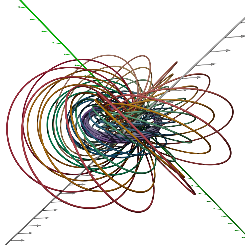
Figure 3: Field lines of the vector field given by equation (21). Every field line is a circle, and all field lines are linked with each other. Two isotropes, stream lines of equation (23), are shown coresponding to the directions $\hat{\mathbf{b}}_{\rm ext}=(0.21,-0.21,0.03)$ (gray) and $-\hat{\mathbf{b}}_{\rm ext}$ (green).

We calculate the isotrope field of the Hopf field by inserting equation (21) into equations (11) and (12). The isotrope field is given by:

$$\boldsymbol{v}=\frac{-4}{(1+r^{2})^{2}\left|-1+x^{2}+y^{2}-z^{2}\right|}\begin{pmatrix}xz-y\\ x+yz\\ 1+z^{2}\\ \end{pmatrix}.$$ (23)

Figure 3 shows select field lines of equation (21). The field consists purely of linked circles lying on a nested toroidal foliation. Two isotropes of the Hopf field, corresponding to $\hat{\mathbf{b}}_{\rm ext}=(0.21,-0.21,0.03)$ (gray) and $-\hat{\mathbf{b}}_{\rm ext}$ (green) are also shown in figure 3. They are integral curves of equation (23), and the arrows along its length are in the direction of $\mathbf{B}_{\rm Hopf}$. The isotropes are straight lines which rule hyperoboid surfaces that form a foliation of $\mathbb{R}^{3}$.

We now can add an external field to the Hopf field, $\mathbf{B}_{\rm Hopf}+B_{0}\hat{\mathbf{b}}_{\rm ext}$. This will create two nulls on the isotrope corresponding with $-\hat{\mathbf{b}}_{\rm ext}$, i.e. the green isotrope in figure 3. In the Hopf field we can study the merger of nulls, unlike in the dipole configuration, where all isotropes intersect at the singularity.

Figure 4 shows the movement of of the nulls as the magnetic field is increased from $B_{0}=0.01$ (a), to $0.065$ (b), $0.2$ (c), and 0.3 (d). As the external field is increased, a positive and a negative null appear from $z=+\infty$ and $z=-\infty$ respectively, and move along the isotrope (still pictured), until they merge on the $z=0$ plane when $B_{0}=0.31$.

\begin{overpic}[width=433.62pt]{hopfnulls.png} \put(1.0,95.0){\fcolorbox{white}{white}{\parbox{7pt}{\centering\textbf{a}}}} \put(51.0,95.0){\fcolorbox{white}{white}{\parbox{7pt}{\centering\textbf{b}}}} \put(1.0,45.0){\fcolorbox{white}{white}{\parbox{7pt}{\centering\textbf{c}}}} \put(51.0,45.0){\fcolorbox{white}{white}{\parbox{7pt}{\centering\textbf{d}}}} \end{overpic}

Figure 4: Movement of nulls in the Hopf field plus a constant external field. The external field is given by $B_{0}\hat{\mathbf{b}}_{\rm ext}$ with the value of $B_{0}$ (a) 0.01, (b) 0.065, (c) 0.2, and (d) 0.3. The external field is opposite the field on the green isotrope in figure 3, and thus the nulls move along it. As the magnitude is increased the two nulls move closer to each other, and merge on the $z=0$ plane. We show the spines as red field lines and the fan planes by a series of blue (northern null) and white (southern null) field lines.

Just as we calculated the isotropes of the Hopf field, we can also calculate the isotropes in this sum field. Instead of deriving an analytical expression for the isotropes, we evaluate the isotrope field numerically using automatic differentiation by implementing equation (12) using the functional transformations in JAX (Bradbury et al., 2018).

The isotrope field of the configurations in figure 4 are shown in figure 5. The northern null is a source for the isotropes, and the southern null is a sink. An isotrope corresponding with every direction will leave the positive null, and one of every direction will enter the negative null. At infinity the Hopf field is zero, and the external field determines the direction of the field. Therefore, only the isotrope corresponding with the external field can go to infinity, all other isotropes connect the one null to the other, like the field lines around two opposite electric charges.

\begin{overpic}[width=433.62pt]{attraction.png} \put(1.0,95.0){\fcolorbox{white}{white}{\parbox{7pt}{\centering\textbf{a}}}} \put(51.0,95.0){\fcolorbox{white}{white}{\parbox{7pt}{\centering\textbf{b}}}} \put(1.0,45.0){\fcolorbox{white}{white}{\parbox{7pt}{\centering\textbf{c}}}} \put(51.0,45.0){\fcolorbox{white}{white}{\parbox{7pt}{\centering\textbf{d}}}} \end{overpic}

Figure 5: Isotrope lines in the sum field $\mathbf{B}_{\rm Hopf}+B_{0}\hat{\mathbf{b}}_{\rm ext}$ during the merger of two nulls. Isotropes from the top null are light green and from the bottom null are dark green. The strength of the external field in panels (a)-(d) are identical to those in the corresponding panels in figure 4. The isotropes emerge from the northern null, and converge on the southern null. As the nulls converge, almost all the isotropes form a short path from one null to the other.

5 Conclusions and Discussion

In this paper we have derived the concept of isotrope lines, lines in space where the magnetic field direction is constant. These lines are integral curves of the isotrope field, which is the Hodge dual of the pull-back of the area two-form on $S^{2}$ over the mapping defined by the direction of the magnetic field. As such, the isotropes convert the topological information of the mapping through which the topological index is defined into a local quantity that can be evaluated everywhere. Isotropes are useful in the analysis of magnetic nulls. Positive nulls are sources and negative nulls are sinks of this field, in a manner analogous to electrical point charges.

In this paper we have used isotropes to analyze the location and movement of nulls in two toy model configurations relevant to astrophysics and plasma physics, namely the dipole and Hopf fields. The nulls that appear are confined to specific isotropes corresponding to the direction opposite the external field.

We also analyzed the merger of two nulls in the Hopf field, both the magnetic structure in terms of the fan and spine planes of the nulls, and the isotrope structure during the merger. With isotropes we can also understand why opposite nulls are ’attracted’ to each other, as they move along isotropes that connect them.

Topological index also applies to higher order nulls, where the first order derivatives become zero, and an analysis in terms of $\boldsymbol{\mathsf{M}}$ breaks down. Though progress has been made in describing such fields using second order derivatives (Yang, 2017; Lukashenko & Veselovsky, 2015), the index provides a unifying framework to classify all nulls. Applying this work to higher order nulls remains for future work.

There are many more applications of the concept of isotropes that did not fit in this paper. Isotropes in two dimensions can be used to locate and predict the movement of X- and O-points in Poincaré sections of magnetic fields in tokamaks and stellarators. In three dimensions, isotropes can be used to locate nulls in numerical simulations, where the isotrope field just needs to be integrated from any starting point to find a null, a process distinct from existing methods.(Olshevsky et al., 2020; Greene, 1992; Haynes & Parnell, 2007, 2010) Development and release of an algorithm for this is the subject of future work. Furthermore, the use of isotropes calculated via interpolation from spacecraft cluster data may offer a novel method for the location of magnetic nulls from this data.(Fu et al., 2015, 2020; Guo et al., 2022; He et al., 2008; Olshevsky et al., 2020)

Appendix A Derivation of the isotrope field in arbitrary dimension

For completeness, and as it may be of interest for broader applications of isotropes, we present a derivation of the expression for the isotrope field corresponding to a vector field in $d$-dimensional Euclidean space.

We take a set of coordinates $\{\phi_{1},\dots\phi_{d-1}\}$ over $S^{d-1}$, and write a volume form over $S^{d-1}$ as

$$\omega=D(\phi_{1},\dots\phi_{d-1})d\phi_{1}\wedge\dots\wedge d\phi_{d-1}.$$ (A1)

The standard choice with spherical coordinates would define $D$ as follows, although we do not require this definition.

$$D(\phi_{1},\dots\phi_{d-1})=\sin^{d-2}(\phi_{1})\sin^{d-3}(\phi_{2})\dots\sin(\phi_{d-2})d\phi_{1}\wedge\dots\wedge d\phi_{d-1}.$$ (A2)

As before, we are seeking some $\boldsymbol{v}$ such that

$$\boldsymbol{v}=\star g^{*}\omega$$ (A3)

where $g(\mathbf{x}):\mathbf{x}\mapsto\left(g_{\phi_{1}}(\mathbf{x})\dots g_{\phi_{d-1}}(\mathbf{x})\right)$ is the map from $\mathbb{R}^{d}$ to $S^{d-1}$ defined by the unit vectors of some vector field $\boldsymbol{V}$.

$$g(\mathbf{x})=\frac{\boldsymbol{V}(\mathbf{x})}{|\boldsymbol{V}(\mathbf{x})|}.$$ (A4)

Consider some hypersurface $Y\subset\mathbb{R}^{d}$, without loss of generality chosen to be $Y=\{\mathbf{x}\in\mathbb{R}^{d}|x_{d}=0\}$. We have

$$\int_{Y}\boldsymbol{v}\cdot da=\int_{Y}g^{*}\omega=\int_{g_{*}Y}\omega=\int_{g_{*}Y}d\phi_{1}\dots d\phi_{d-1}D(\phi_{1},\dots\phi_{d-1}).$$ (A5)

Pulling this integral back into $Y$ from $S^{d-1}$ and taking the corresponding coordinate transformation:

$$\int_{Y}g^{*}\omega=\int_{Y}dx_{1}\dots dx_{d-1}\epsilon^{i_{1}\dots i_{d-1}}(\partial_{x_{1}}g_{\phi_{i_{1}}})\dots(\partial_{x_{d-1}}g_{\phi_{i_{d-1}}})D(g_{\phi_{1}},\dots g_{\phi_{d-1}}),$$ (A6)

from which we conclude:

$$g^{*}\omega(\mathbf{a}_{1},\dots\mathbf{a}_{d-1})=\epsilon^{i_{1}\dots i_{d-1}}(\partial_{\mathbf{a}_{1}}g_{\phi_{i_{1}}})\dots(\partial_{\mathbf{a}_{d-1}}g_{\phi_{i_{d-1}}})D(g_{\phi_{1}},\dots g_{\phi_{d-1}}).$$ (A7)

We can then compute the components of $\boldsymbol{v}$. We start from the formula:

$$\boldsymbol{v}=\star g^{*}\omega.$$ (A8)

Applying the definition of the Hodge dual and contracting $g^{*}\omega$ with vectors $\boldsymbol{a}_{1},\dots\boldsymbol{a}_{d-1}$,

$$\begin{split}\epsilon_{j_{1}\dots j_{d}}a_{1}^{j_{1}}\dots a_{d-1}^{j_{d-1}}v^{j_{d}}=&g^{*}\omega(\mathbf{a}_{1},\dots\mathbf{a}_{d-1})\\ =&\epsilon^{i_{1}\dots i_{d-1}}(\partial_{\mathbf{a}_{1}}g_{\phi_{i_{1}}})\dots(\partial_{\mathbf{a}_{d-1}}g_{\phi_{i_{d-1}}})D(g_{\phi_{1}},\dots g_{\phi_{d-1}})\\ \epsilon_{j_{1}\dots j_{d}}a_{1}^{j_{1}}\dots a_{d-1}^{j_{d-1}}v^{j_{d}}=&\epsilon^{i_{1}\dots i_{d-1}}\left(a_{1}^{j_{1}}\partial_{j_{1}}g_{\phi_{i_{1}}}\right)\dots\left(a_{d-1}^{j_{d-1}}\partial_{j_{d-1}}g_{\phi_{i_{d-1}}}\right)D(g_{\phi_{1}},\dots g_{\phi_{d-1}}).\end{split}$$ (A9)

As $a_{1}^{j_{1}}\dots a_{d-1}^{j_{d-1}}$ is entirely general, we can remove it from both sides, yielding

$$\epsilon_{j_{1}\dots j_{d}}v^{j_{d}}=\epsilon^{i_{1}\dots i_{d-1}}\left(\partial_{j_{1}}g_{\phi_{i_{1}}}\right)\dots\left(\partial_{j_{d-1}}g_{\phi_{i_{d-1}}}\right)D(g_{\phi_{1}},\dots g_{\phi_{d-1}})$$ (A10)

We now multiply both sides by $\epsilon^{j_{1}\dots j_{d-1}k}$ and simplify

$$\begin{split}\epsilon^{j_{1}\dots j_{d-1}k}\epsilon_{j_{1}\dots j_{d}}v^{j_{d}}=&\epsilon^{j_{1}\dots j_{d-1}k}\epsilon^{i_{1}\dots i_{d-1}}\left(\partial_{j_{1}}g_{\phi_{i_{1}}}\right)\dots\left(\partial_{j_{d-1}}g_{\phi_{i_{d-1}}}\right)D(g_{\phi_{1}},\dots g_{\phi_{d-1}})\\ =&(d-1)!\ \delta^{k}_{j_{d}}v^{j_{d}},\end{split}$$ (A11)

yielding the components of $\boldsymbol{v}$:

$$v^{k}=\frac{1}{(d-1)!}\epsilon^{j_{1}\dots j_{d-1}k}\epsilon^{i_{1}\dots i_{d-1}}\left(\partial_{j_{1}}g_{\phi_{i_{1}}}\right)\dots\left(\partial_{j_{d-1}}g_{\phi_{i_{d-1}}}\right)D(g_{\phi_{1}},\dots g_{\phi_{d-1}}).$$ (A12)

This vector field can be proven to point along isotropes as follows.

$$\begin{split}\boldsymbol{v}\cdot\nabla g_{\phi_{l}}=v^{k}\partial_{k}g_{\phi_{l}}=\frac{1}{(d-1)!}\epsilon^{j_{1}\dots j_{d-1}k}\epsilon^{i_{1}\dots i_{d-1}}\left(\partial_{j_{1}}g_{\phi_{i_{1}}}\right)\dots\left(\partial_{j_{d-1}}g_{\phi_{i_{d-1}}}\right)\left(\partial_{k}g_{\phi_{l}}\right)D(g_{\phi_{1}},\dots g_{\phi_{d-1}}).\end{split}$$ (A13)

For any nonzero term in this sum, there must be one element of the multi-index $\{i_{1},\dots i_{d-1}\}$ that equals $l$. Without loss of generality, consider the case $i_{d-1}=l$.

$$\begin{split}\epsilon^{j_{1}\dots j_{d-1}k}\left(\partial_{j_{d-1}}g_{\phi_{l}}\right)\left(\partial_{k}g_{\phi_{l}}\right)=&\frac{1}{2}\left(\epsilon^{j_{1}\dots j_{d-1}k}-\epsilon^{j_{1}\dots j_{d-2}kj_{d-1}}\right)\left(\partial_{j_{d-1}}g_{\phi_{l}}\right)\left(\partial_{k}g_{\phi_{l}}\right)\\ =&\frac{1}{2}\epsilon^{j_{1}\dots j_{d-1}k}\left(\left(\partial_{j_{d-1}}g_{\phi_{l}}\right)\left(\partial_{k}g_{\phi_{l}}\right)-\left(\partial_{k}g_{\phi_{l}}\right)\left(\partial_{j_{d-1}}g_{\phi_{l}}\right)\right)\\ =&0.\end{split}$$ (A14)

Therefore, all terms in equation (A13) must vanish, and $\boldsymbol{v}$ is orthogonal to the gradients of all components of $g$. The coordinates are constant along stream lines of $\boldsymbol{v}$, i.e. $\boldsymbol{v}$ defines the isotrope field.

Appendix B Straightening External fields

Our goal is to demonstrate a means of constructing a coordinate transformation which preserves the topology of vector fields and which yields a basis in which an arbitrary magnetic field is constant. This method is applicable so long as all field lines start and end on the boundary of the domain under consideration. We begin by noting that a vector field has constant coefficients in a particular coordinate system precisely when it commutes (with respect to the Lie bracket) with the basis vector fields. We can generate a vector field $\mathbf{X}$ that commutes with a given magnetic field $\mathbf{B}$ by choosing its values on some surface and Lie dragging it along the magnetic fieldlines passing through the surface. This amounts to integrating the differential equation

$$B_{i}\left(\partial_{i}X_{j}\right)=\left(\partial_{i}B_{j}\right)X_{i}.$$ (B1)

for a particular choice of Cauchy data, which by definition gives a solution such that $[\mathbf{B},\mathbf{X}]_{j}=B_{i}\left(\partial_{i}X_{j}\right)-\left(\partial_{i}B_{j}\right)X_{i}=0$. By choosing two commuting vector fields $\mathbf{X}$, $\mathbf{Y}$ lying on the boundary such that $\mathbf{B}\cdot\mathbf{X}\times\mathbf{Y}=1$ and Lie dragging as above, we construct a coordinate basis $\left\{\mathbf{X},\mathbf{Y},\mathbf{B}\right\}$ in which $\mathbf{B}=(0,0,1)$ everywhere. Note that their mutual commutation is required for the vector fields to generate consistent coordinates.
This process can also be considered from the perspective of matrix transformations on tangent spaces of $\mathbb{R}^{3}$. Equation B1 can be written

$$\frac{d}{ds}\mathbf{X}=\boldsymbol{\mathsf{M}}\cdot\mathbf{X}.$$ (B2)

where $s$ is a fieldline parameter such that $\frac{dx_{i}}{ds}=B_{i}$ and $\mathsf{M}_{ij}=\partial_{j}B_{i}$ is the Jacobian of the magnetic field. We are seeking some transformation matrix $\boldsymbol{\mathsf{T}}(x)\in SL(3,\mathbb{R})$ that maps an initial vector on the boundary to its Lie dragging to some point $\mathbf{x}$: $\mathbf{X}(\mathbf{x})=\boldsymbol{\mathsf{T}}(\mathbf{x})\cdot\mathbf{X}_{0}$. This yields

$$\frac{d}{ds}\boldsymbol{\mathsf{T}}=\boldsymbol{\mathsf{M}}\cdot\boldsymbol{\mathsf{T}},$$ (B3)

with the solution

$$\boldsymbol{\mathsf{T}}=\mathcal{T}\left\{e^{\int\boldsymbol{\mathsf{M}}ds}\right\}=\sum_{n=0}^{\infty}\int_{0}^{L}\int_{0}^{s_{n}}\int_{0}^{s_{n-1}}...\int_{0}^{s_{2}}\boldsymbol{\mathsf{M}}(s_{n})...\boldsymbol{\mathsf{M}}(s_{1})ds_{1}...ds_{n}$$ (B4)

where $\mathcal{T}$ denotes the time-ordering of the integral along the path. Noting that $\int\mathsf{M}_{ij}ds=\int\mathsf{M}_{ij}\mathbf{B}\cdot dl$, we see that we are integrating a Lie algebra valued one form $\mathsf{M}_{ij}B_{\alpha}:T\mathbb{R}^{3}\rightarrow\mathfrak{sl}(3,\mathbb{R})$ over a curve that happens to be the streamline of the magnetic field. The resulting matrix in $SL(3,\mathbb{R})$ defines a basis transformation at the end point (and at any intermediate point along the path) that maps $\mathbf{B}$ at the start point to $\mathbf{B}$ at the endpoint and functions to Lie drag vectors. This means of transporting vector fields along field lines might be extended to arbitrary paths, producing a gauge connection on the tangent bundle.

Appendix C Jacobian of the dipole field

Here we briefly show for completeness that the Jacobian of a dipole field with moment pointed along $\hat{z}$ is negative for $z>0$ and positive for $z<0$. Written in Cartesian coordinates, the unit dipole field is

$$\mathbf{B}=\left(\frac{3xz}{\left(x^{2}+y^{2}+z^{2}\right)^{5/2}},\frac{3yz}{\left(x^{2}+y^{2}+z^{2}\right)^{5/2}},\frac{2z^{2}-x^{2}-y^{2}}{\left(x^{2}+y^{2}+z^{2}\right)^{5/2}}\right)$$ (C1)

with Jacobian

$$\boldsymbol{\mathsf{M}}=\frac{1}{(x^{2}+y^{2}+z^{2})^{7/2}}\left(\begin{array}[]{ccc}3z\left(-4x^{2}+y^{2}+z^{2}\right)&-15xyz&3x\left(x^{2}+y^{2}-4z^{2}\right)\\ -15xyz&3z\left(x^{2}-4y^{2}+z^{2}\right)&3y\left(x^{2}+y^{2}-4z^{2}\right)\\ 3x\left(x^{2}+y^{2}-4z^{2}\right)&3y\left(x^{2}+y^{2}-4z^{2}\right)&9x^{2}z+9y^{2}z-6z^{3}\\ \end{array}\right).$$ (C2)

The determinant is

$$|\boldsymbol{\mathsf{M}}|=-\frac{27z\left(x^{2}+y^{2}+2z^{2}\right)}{\left(x^{2}+y^{2}+z^{2}\right)^{15/2}}.$$ (C3)

From equation (C3) it is clear that ${\rm sign}\left(|\boldsymbol{\mathsf{M}}|\right)=-{\rm sign}(z)$

References

- Bradbury et al. (2018) Bradbury, J., Frostig, R., Hawkins, P., et al. 2018, JAX: composable transformations of Python+NumPy programs, 0.3.13. http://github.com/google/jax
- Brouwer (1911) Brouwer, L. E. J. 1911, Mathematische Annalen, 71, 97
- Candelaresi (2016) Candelaresi, S. 2016, SPD, 401
- Cowley (1973) Cowley, S. 1973, Radio Science, 8, 903
- Degnan et al. (1993) Degnan, J., Peterkin Jr, R., Baca, G., et al. 1993, Physics of Fluids B: Plasma Physics, 5, 2938
- Doyle (1892) Doyle, A. C. 1892, The Adventure of Silver Blaze (Strand Magazine)
- Elder & Boozer (2021) Elder, T., & Boozer, A. H. 2021, Journal of Plasma Physics, 87, 905870225, doi: 10.1017/S0022377821000210
- Finkelstein & Weil (1978) Finkelstein, D., & Weil, D. 1978, International Journal of Theoretical Physics, 17, 201
- Fu et al. (2020) Fu, H., Wang, Z., Zong, Q., et al. 2020, Dayside Magnetosphere Interactions, 153
- Fu et al. (2015) Fu, H. S., Vaivads, A., Khotyaintsev, Y. V., et al. 2015, Journal of Geophysical Research: Space Physics, 120, 3758, doi: 10.1002/2015JA021082
- Greene (1988) Greene, J. M. 1988, Journal of Geophysical Research: Space Physics (1978–2012), 93, 8583
- Greene (1992) —. 1992, Journal of Computational Physics, 98, 194
- Guo et al. (2022) Guo, R., Pu, Z., Wang, X., Xiao, C., & He, J. 2022, Journal of Geophysical Research: Space Physics, 127, e2021JA030248, doi: 10.1029/2021JA030248
- Haynes & Parnell (2007) Haynes, A. L., & Parnell, C. E. 2007, Physics of Plasmas, 14, 082107, doi: 10.1063/1.2756751
- Haynes & Parnell (2010) —. 2010, Physics of Plasmas, 17, 092903, doi: 10.1063/1.3467499
- He et al. (2008) He, J.-S., Tu, C.-Y., Tian, H., et al. 2008, Journal of Geophysical Research: Space Physics, 113, doi: 10.1029/2007JA012609
- Hopf (1931) Hopf, H. 1931, Math. Ann., 104, 637
- Kamchatnov (1982) Kamchatnov, A. M. 1982, Soviet Journal of Expermental and Theoretical Physics, 82, 117
- Lau & Finn (1990) Lau, Y.-T., & Finn, J. M. 1990, The Astrophysical Journal, 350, 672
- Lukashenko & Veselovsky (2015) Lukashenko, A., & Veselovsky, I. 2015, Geomagnetism and Aeronomy, 55, 1152
- Murphy et al. (2015) Murphy, N. A., Parnell, C. E., & Haynes, A. L. 2015, Physics of Plasmas, 22, 102117
- Olshevsky et al. (2020) Olshevsky, V., Pontin, D., Williams, B., et al. 2020, Astronomy & Astrophysics, 644, A150
- Parnell et al. (1996) Parnell, C., Smith, J., Neukirch, T., & Priest, E. 1996, Physics of Plasmas (1994-present), 3, 759
- Priest & Titov (1996) Priest, E. R., & Titov, V. 1996, Philosophical Transactions of the Royal Society of London. Series A: Mathematical, Physical and Engineering Sciences, 354, 2951
- Ranada (1992) Ranada, A. F. 1992, Journal of Physics A: Mathematical and General, 25, 1621, doi: 10.1088/0305-4470/25/6/020
- Schindler et al. (1988) Schindler, K., Hesse, M., & Birn, J. 1988, Journal of Geophysical Research: Space Physics, 93, 5547
- Smiet et al. (2015) Smiet, C., Candelaresi, S., Thompson, A., et al. 2015, Physical review letters, 115, 095001
- Smiet et al. (2019a) Smiet, C., de Blank, H., de Jong, T., Kok, D., & Bouwmeester, D. 2019a, Journal of Plasma Physics, 85
- Smiet et al. (2019b) Smiet, C., Kramer, G., & Hudson, S. 2019b, Plasma Physics and Controlled Fusion, 62, 025007
- Tanaka et al. (2022) Tanaka, T., Ebihara, Y., Watanabe, M., et al. 2022, Journal of Geophysical Research: Space Physics, 127, e2022JA030332
- Tuszewski (1988) Tuszewski, M. 1988, Nuclear Fusion, 28, 008
- Winslow et al. (2012) Winslow, R. M., Johnson, C. L., Anderson, B. J., et al. 2012, Geophysical Research Letters, 39
- Yang (2017) Yang, S.-D. 2017, Physics of Plasmas, 24, 012903
- Yu & Egedal (2022) Yu, X., & Egedal, J. 2022, Bulletin of the American Physical Society