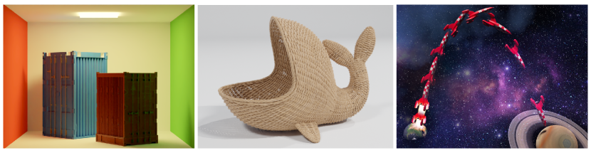
Figure 1. Our method optimizes arbitrary black-box graphics pipelines, such as rendering (left: finding the box and light position under a discontinuous integrand), modelling (middle: combinatorical count of vertical and horizontal wicker stakes), and animation (right: optimal control of the engine turn-off time), which all do not provide gradients. Please see Fig. 10 and Fig. 11 for initializations and convergence of our and other methods on these very problems.

Zero Grads Ever Given:
Learning Local Surrogate Losses for Non-Differentiable Graphics

Abstract.

Gradient-based optimization is now ubiquitous across graphics, but unfortunately can not be applied to problems with undefined or zero gradients. To circumvent this issue, the loss function can be manually replaced by a “surrogate” that has similar minima but is differentiable. Our proposed framework, ZeroGrads, automates this process by learning a neural approximation of the objective function, the surrogate, which in turn can be used to differentiate through arbitrary black-box graphics pipelines. We train the surrogate on an actively smoothed version of the objective and encourage locality, focusing the surrogate’s capacity on what matters at the current training episode. The fitting is performed online, alongside the parameter optimization, and self-supervised, without pre-computed data or pre-trained models. As sampling the objective is expensive (it requires a full rendering or simulator run), we devise an efficient sampling scheme that allows for tractable run-times and competitive performance at little overhead. We demonstrate optimizing diverse non-convex, non-differentiable black-box problems in graphics, such as visibility in rendering, discrete parameter spaces in procedural modelling or optimal control in physics-driven animation. In contrast to more traditional algorithms, our approach scales well to higher dimensions, which we demonstrate on problems with up to 35k interlinked variables.

1. Introduction

Gradient-based optimization has recently become an essential part of many Graphics applications, ranging from rendering to find light or reflectance [Fischer and Ritschel, 2022a; Rainer et al., 2019; Gardner et al., 2019], over procedural material modelling [Hu et al., 2022a] to animation of characters or fluids [Habermann et al., 2021; Schenck and Fox, 2018]. These methods provide state of the art results, in particular when combined with large amounts of training data and neural networks that represent the desired mappings or assets. In order to train these methods via gradient descent (GD), the pipeline needs to be fully differentiable, allowing to backpropagate gradients from the objective function to the optimization parameters. This often is enabled by intricate, task-specific derivations [Loubet et al., 2019; Li et al., 2018] or requires fundamental changes to the pipeline, such as the switch to a dedicated programming language [Bangaru et al., 2021; Hu et al., 2019].

In practice, the application of these ideas remains limited, as many existing graphics pipelines are black boxes (e.g., entire 3D modelling packages such as Blender or rendering pipelines such as Renderman [Christensen et al., 2018] or Unity [Haas, 2014]) that do not provide access to their internal workings and hence cannot be differentiated. Further, even if we were given access to the pipeline’s internals, the employed functions might not be differentiable (e.g., the step function) or provide gradients that are insufficient for convergence [Metz et al., 2021]. The mindset of this article is that we only have access to a forward model, e.g., a modeling pipeline, and a reference, e.g., a target image. Using these two, a loss can be computed – its gradients, however, cannot be used.

If a loss is not differentiable in practice, it can be approximated by a “surrogate” loss (Fig. 2). The surrogate is a function that has similar minima as the true loss, but also provides gradients that are useful when employed in an optimization. While the concept of surrogate modelling is not new (cf. Sec. 2), it remains unclear how to efficiently find a surrogate loss for any arbitrary graphics pipeline, as here the sampling must be sparse (recall, rendering a sample is expensive), and the problems at hand can reach high dimensionality (up to several thousand interlinked optimization variables). In this article, we thus propose ZeroGrads, a systematic and efficient way of learning local surrogate losses, requiring no more than a forward model and a reference.

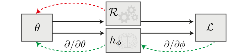
Figure 2. Regular forward models might not be able to provide gradients w.r.t. their input parameters $\theta$ (red arrow, top). Our approach, ZeroGrads, provides this ability via a local learned surrogate (green arrows, bottom) that maps $\theta$ to the associated loss and can be differentiated analytically.

To learn our surrogate loss and use it in an optimization, we follow four key steps: We first smooth the original loss by convolving the cost landscape with a blur kernel, so that it provides gradients that lead to (improved) convergence when used during GD. We secondly fit a surrogate, a parametric function such as a neural network or a quadratic potential, to that smoothed loss. As the surrogate is differentiable by construction, we can query it to get surrogate gradients that drive the parameter optimization. We thirdly constrain this fit to the local neighbourhood of the current parameters, as the global cost landscape is in large parts irrelevant for the current optimization step. By locally updating our surrogate, we allow it to focus on what matters “around” the current solution. However, querying the objective function to create samples for our surrogate fitting is expensive, as each sample requires the execution of the full forward model, such as a light transport simulation or physics solver. Therefore, fourth and finally, we derive an efficient sampler that reduces the variance of the surrogate’s gradient estimates and thus allows us to use ZeroGrads with a low number of sparse samples at tractable runtimes. Our local surrogate losses hence can be trained online alongside the actual parameter optimization, and self-supervised, without the need for pre-trained models or pre-computed ground truth gradients. Our sparse low-variance sampling strategy allows our surrogates to scale up to very high dimensions. We demonstrate ZeroGrads on a variety of tasks across different domains, ranging from differentiable rendering over procedural modelling to physical animation. In summary, our contributions are:

• ZeroGrads, a framework that maps a forward model without usable gradients into a smooth, differentiable surrogate function, such as an NN, with analytic gradients.

• Reducing the variance of surrogate updates to allow tractable runtimes and unsupervised on-the-fly optimization.

• Optimizing several non-differentiable black-box graphics problems from rendering (visibility) over modelling (discrete procedurals) to simulation and animation (binary control).

• Showing that our surrogates favourably scale to higher dimensions, where existing derivative-free methods often struggle to converge.

We would like to emphasize that we do not claim superiority (less variance, better convergence, …) over existing, specialized methods such as Mitsuba [Jakob et al., 2022], Redner [Li et al., 2018] or PhiFlow [Holl et al., 2020], but rather broaden the spectrum of inverse graphics by now enabling gradient-based optimization on arbitrary, non-differentiable graphics pipelines.

2. Previous Work

Optimization in graphics

Parameters of graphics models are now routinely optimized so as to fulfill user-provided goals. The two main ingredients enabling this are gradient-based optimization and tunable architectures. We will not consider the many different exciting architectures in this work, but focus on the optimization itself. Gradients are typically computed by using a language that allows efficient auto-differentiation, such as PyTorch [Paszke et al., 2017] or JAX [Bradbury et al., 2018], often targeting GPUs. Unfortunately, several problems in graphics are not differentiable.

Methods that do not rely on gradients [Rios and Sahinidis, 2013], such as asking a user [Marks et al., 1997], global optimization [Jones et al., 1998], direct search [Powell, 1994], simulated annealing (SA) [Kirkpatrick et al., 1983], simultaneous perturbation stochastic approximation (SPSA) [Spall, 1992], particle swarms [Parsopoulos and Vrahatis, 2002] or genetic algorithms [Holland, 1973] have largely fallen from favour in everyday graphics use. This is partially due to the fact that gradient-free optimization – even on smooth problems – often requires a large number of function evaluations before converging [Jamieson et al., 2012], and, in general, struggles with convergence as problem dimensionality increases. Additionally, gradient-free optimizers often suffer from high per-iteration cost in higher dimensions (e.g., finite differences (FD) or [Zhang et al., 2020]), or require the computation of the Hessian matrix in Newton-type methods, leading to a trade-off in scalability and performance. GD, in contrast, has strong convergence guarantees (under convex objectives), is highly scalable, can be parallelized effectively, and has shown superior performance in high-dimensional settings (e.g., NN training). Unfortunately, it cannot be used on many relevant problems (although the cost landscape itself might be smooth), as many graphics pipelines are simply not designed to be differentiable. Our approach circumvents this issue by providing surrogate gradients that GD can work with. Even for non-smooth problems, our formulation makes the problem smooth and hence amenable to GD.

Differentiation

Most graphics pipelines used in production (e.g., Blender, GIMP, Photoshop) are not differentiable, as they are not implemented in a differentiable programming language. The deeper underlying mathematical problem is that their output often relies on integration – however, differentiation and the typical integral estimation through Monte Carlo (MC) cannot be interchanged without further considerations. A prominent example are discontinuities in rendering, which have sparked a body of work by Lee et al. [2018]; Bangaru et al. [2021]; Loper and Black [2014]; Kato et al. [2018]; Li et al. [2018]; Liu et al. [2019]; Rhodin et al. [2015]; Xing et al. [2022] or Loubet et al. [2019], to only name a few salient ones. Similar problems appear in vector graphics [Li et al., 2020], signed distance functions [Vicini et al., 2022; Bangaru et al., 2022], entire programs [Chandra et al., 2022] or physics [Hu et al., 2019; Chang et al., 2016; Mrowca et al., 2018]. All these approaches require access to the internals of the graphics pipeline in order to replace or change parts such that gradients can be backpropagated. Our approach, in contrast, assumes the pipeline to be a black box and does not make any assumptions or approximations to the internals.

Proxies

A key insight is that we only need the loss’ gradients, and not those of the entire pipeline. Hence, if a part in a conventional graphics pipeline cannot be differentiated, we search for a similar function that we can differentiate instead, our proxy. As the proxy is an analytic function, its gradients can readily be computed via automatic differentiation (AD) and then be used to drive the optimization. Graphics is a good fit for neural proxies, as we can freely sample the objective in many cases, e.g., by rendering an image or running a simulation (a “simulation-optimization” setting [Law et al., 2007]). While easy to do, still, creating a sample is expensive.

The concept of “Neural Proxies” was pioneered for physics by Grzeszczuk et al. [1998] and is now applied to problems such as material editing [Hu et al., 2022a], photo editing [Tseng et al., 2022; Fischer et al., 2020], hardware design [Tseng et al., 2019], software synthesis [Esmaeilzadeh et al., 2012], simulation [Munk et al., 2019; Renda et al., 2020] or animation [Shirobokov et al., 2020; Navrátil et al., 2019; Sin et al., 2021]. Rendering itself becomes differentiable when replaced by a NN proxy [Nalbach et al., 2017], however, having a NN emulate the complex behaviour of a full graphics pipeline might be overambitious and will not scale to complex assets.

Surrogate losses

Surrogate losses [Queipo et al., 2005] (sometimes also called meta-models [Barton, 1994; Box and Draper, 1987]) extend the idea of proxies by providing an approximation to the entire forward model’s behaviour by only emulating its response (or loss landscape), without necessarily replicating all the internals of a graphics pipeline. Differentiating the surrogate will provide gradients which can then be used to drive a (gradient-based) optimization algorithm. Surrogates are especially popular when taking a sample is expensive, like in airplane design [Forrester and Keane, 2009] or neural architecture search [Zhou et al., 2020], and can be modelled in a number of ways, e.g., through polynomials [Jones et al., 1998], radial basis functions [Gutmann, 2001] and recently, neural networks [Grabocka et al., 2019; Patel et al., 2020]. Most of these methods learn surrogates for the entire cost landscape (typically in a simplified setting, e.g., classification), with the exception of response surface maps, which fit a first- or second order polynomial to the local neighbourhood, but are known to not converge on higher-dimensional problems [Wan et al., 2005]. More crucially, aside from global fitting, most methods assume the availability of a large set of data samples, e.g., a curated image collection like ImageNet [Deng et al., 2009]. In our setting, in contrast, sampling is expensive, which is why we sample sparsely and locally and fit the surrogate in-the-loop, during optimization, thereby allowing our surrogates to scale to the full landscape of optimization tasks and high dimensions.

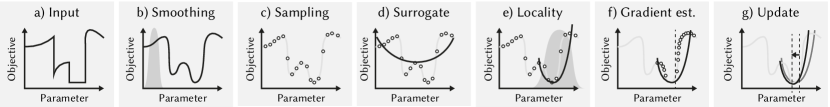
Figure 3. A conceptual illustration of our approach; each subplot shows a one-dimensional cost landscape. For details please refer to Sec. 3: Overview.

Gradient estimation

Ironically, the surrogate itself is updated gradient-based, by sampling the objective function a finite number of times and then estimating the surrogate’s gradient from its prediction error. For general learning, building gradients is fundamentally a MC estimation problem [Mohamed et al., 2020], akin to what Graphics routinely is solving for production rendering [Veach, 1998]. We identify the similarity of estimating proxy gradients and simulating light transport (high dimensionality, sparsity, product integrands) and employ variance reduction based on importance sampling [Veach, 1998; Kahn, 1950; Kajiya, 1986] to increase the efficiency of our surrogate gradient estimates.

3. Our approach

Given a scalar objective function $f(\theta)\!:\Theta\rightarrow\mathbb{R}_{0}^{+}$ varying over an $n$ -dimensional parameter space $\Theta$ , we would like to find the optimal parameters $\theta^{*}$ that minimize $f$ . Typically, gradient-based optimizers such as SGD or ADAM are used for such a task. However, in the setting of this work, their direct use is not possible, as the objective’s gradients $\partial f/\partial\theta$ are either not accessible (in a black box pipeline), undefined (at discontinuities), zero (on a plateau) or too costly to compute (e.g., when appearing in an integral). We are, however, able to sample this objective function by sampling a set of parameters and then comparing the resulting output with the reference. We propose to now locally fit a tunable and differentiable surrogate function $h(\theta,\phi)$ to those samples, whose derivative $\partial h/\partial\theta$ will act as surrogate gradient and drive the optimization.

Overview

Our approach is summarized in Alg. 1 and Fig. 3. Given an arbitrary (potentially non-smooth and non-convex) objective function (Fig. 3 a, also called loss landscape) and a randomly initialized parameter state $\theta$ , we first smooth the objective via convolution with a Gaussian kernel in order to reduce plateaus (Sec. 3.1 and Fig. 3 b). We subsequently fit our surrogate $h$ (Sec. 3.2) to this smooth objective. However, sampling is expensive (requiring a full rendering or simulator run), and global sampling and surrogate fitting would be very approximate (cf. Fig. 3 c, d), which is why we enforce locality via another Gaussian kernel (Fig. 3 e and Sec. 3.3) and hence encourage the surrogate to focus on what matters at the current optimization iteration. Unfortunately, we do not have supervision gradients to train our surrogate with, which is why we resort to estimating the surrogate’s gradient (Sec. 3.4). As is common in NN training, some samples are more informative than others, but in this case it is unclear how to find those, i.e., how we can efficiently sample in this convolved space. To this end, we derive an efficient importance-sampler (Fig. 3 f and Sec. 3.5) that samples according to the locality terms and thus reduces the variance of the estimated surrogate gradient. Finally, we use this estimated gradient to update our surrogate (Fig. 3 g) in order to improve its fit to the objective. We can then descend along the surrogate’s gradient $\partial h/\partial\theta$ (readily available via AD) to update the optimization parameter $\theta$ and repeat the process from b) onward, i.e., the surrogate is updated from its previous state instead of re-fit. Lines 5 and 6 in Alg. 1 illustrate this, where Optimize performs gradient descent steps on a variable.

Algorithm 1 High-level pseudo-code of ZeroGrads.

1:procedure ZeroGrads($f$ , $h$ )

2:     $\phi$ := Uniform() $\triangleright$ surrogate parameters

3:     $\theta$ := Uniform() $\triangleright$ optimization parameters

4:     for i do

5:         $\phi$ = Optimize₁($\phi$ , EstimateGradient($\phi$ , $\theta$ $f$ , $h$ ))

6:         $\theta$ = Optimize₂($\theta$ , $\frac{\partial h}{\partial\theta}$)

7:     end for

8:end procedure

3.1. Smooth objective

As the objective might not always be differentiable (or provide gradients that are of little use [Metz et al., 2021]), we seek to find a function that has similar optima and is differentiable. In practice, the issue is not so much point singularities where the function is not differentiable (those are even present in the acclaimed ReLU), but regions with zero gradients (“plateaus”). These can be removed by convolving the objective with a blur kernel. Similar tricks have been applied to rasterization [Liu et al., 2019; Petersen et al., 2022] and path-tracing [Fischer and Ritschel, 2022b], which we scale to arbitrary spaces. We define the smooth objective $g(\theta)\!:\Theta\rightarrow\mathbb{R}_{0}^{+}$ as

(1) $$g(\theta)=\kappa*f(\theta)=\int_{\Theta}\kappa(\tau)f(\theta-\tau)\mathrm{d}\tau,$$

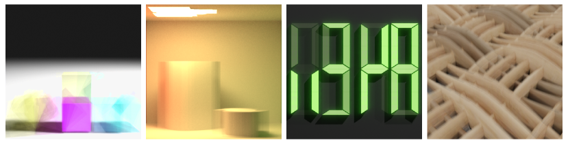
Figure 4. Samples of the smooth objective on which we learn our surrogate: Perturbing the scene parameters smooths discontinuities, e.g., the binary on/off for the LED task (an inset is shown).

a convolution of the objective $f$ and a smoothing kernel $\kappa$ , which we choose to be a Gaussian. Convolution with a Gaussian kernel has several desirable properties, e.g., convexity is preserved, it holds that $L_{g}\leq L_{f}$, i.e., the smooth objective is stronger Lipschitz-bound than $f$ , and the gradient $\nabla_{g}$ is Lipschitz-continuous even when $\nabla_{f}$ is not [Nesterov and Spokoiny, 2017], as is the case on many of our problems (e.g., Fig. 3 a)). We show visualizations of Eq. 1 in Fig. 4.

3.2. Surrogate

The key ingredient, the surrogate $h(\theta,\phi)\!:\Theta\,\times\,\Phi\rightarrow\mathbb{R}_{0}^{+}$ , consumes $\theta$ (like $f$ and $g$ , which it emulates), but also takes the tunable parameters $\phi$ from the $m$ -dimensional surrogate parameter space $\Phi$ .

We encode our surrogate in a differentiable proxy function of variable form, ranging from polynomials over RBFs to NNs. We will give examples of this in the evaluation in Sec. 4.4. Thanks to this analytic parametrization, we can easily get the surrogate gradient $\partial h/\partial\phi$ and the parameter gradient $\partial h/\partial\theta$ using automatic differentiation. In contrast to linear methods (e.g., [Zhang et al., 2020; Fischer and Ritschel, 2022b]), our continuous surrogate formulation allows us to perform one or more gradient descent steps on the surrogate.

3.3. Localized surrogate loss

Matching $h$ to $g$ across the entire domain $\Theta$ might be too ambitious and furthermore is unnecessary, as most first-order gradient-based optimizers only ever query values at or around the current parameter $\theta$ . Instead, we create a surrogate that is focused around the current parameters by locally sampling the objective function.

The loss of the surrogate parameters $\phi$ “around” $\theta$ hence is

(2) $$l(\theta,\phi)=\int_{\Theta}\lambda(\rho,\theta)\left(g(\rho)-h(\rho,\phi)\right)^{2}\mathrm{d}\rho,$$

where $\lambda$ is a weighting function that chooses how much context is considered around the current solution and $\rho$ is from the parameter space $\Theta$ . We again choose a Gaussian with mean $\theta$ here, which is not to be confused with the smoothing kernel $\kappa$ . Eq. 2 nicely shows how the surrogate never has access to the gradients of the true objective – these might not even exist –, but learns self-supervised by only sampling the (smoothed) loss $g$ .

3.4. Estimator

Combining the smoothed loss in Eq. 1 and the localized surrogate loss in Eq. 2, we arrive at the following expression:

(3) $$l(\theta,\phi)=\int_{\Theta}\underbrace{\lambda(\rho,\theta)\left(\left[\int_{\Theta}\kappa(\tau)f(\rho-\tau)\mathrm{d}\tau\right]-h(\rho,\phi)\right)^{2}}_{:=I(\rho,\,\phi)}\mathrm{d}\rho.$$

We are now interested in the gradient of this expression w.r.t. the surrogate parameters $\phi$ , i.e.,

(4) $$\frac{\partial}{\partial\phi}l(\theta,\phi)=\frac{\partial}{\partial\phi}\int_{\Theta}I(\rho,\phi)\mathrm{d}\rho=\int_{\Theta}\frac{\partial}{\partial\phi}I(\rho,\phi)\mathrm{d}\rho.$$

The above equality holds, according to Leibniz’ rule of differentiation under the integral sign, if, and only if, the integrand is continuous in $\phi$ and $\rho$ [Li et al., 2018]. Our Gaussian locality weight $\lambda$ fulfills this and $h(\rho,\phi)$ is continuous by definition, as it is a NN or quadratic potential. Through our previously introduced convolution (Eq. 1), the – originally discontinuous – objective $f$ becomes smooth and hence leads to the inner integral being continuous in $\rho$ .

Leveraging the fact that a composition of continuous functions also is continuous, we can say that $I(\rho,\phi)$ is continuous in $\phi$ and hence use Eq. 4 as our gradient estimator:

(5) $$\frac{\partial}{\partial\phi}l =\int_{\Theta}\frac{\partial}{\partial\phi}\lambda(\rho,\theta)\left(\left[\int_{\Theta}\kappa(\tau)f(\rho-\tau)\mathrm{d}\tau\right]-h(\rho,\phi)\right)^{2}\mathrm{d}\rho$$

(6) $$=\int_{\Theta}2\lambda(\rho,\theta)\frac{\partial h(\rho,\phi)}{\partial\phi}\left(h(\rho,\phi)-\int_{\Theta}\kappa(\tau)f(\rho-\tau)\mathrm{d}\tau\right)\mathrm{d}\rho.$$

Here, the inner integral over $\tau$ is conditioned on the outer variable $\rho$ , leading to a nested integration problem. A naïve solution would estimate the inner integral with $N$ independent samples for each of the $M$ outer samples, leading to quadratic complexity $\mathcal{O}(N\times M)$.

We now aim to re-arrange Eq. 6 into a double-integral of a product, a form that is reliably solvable by the well-known approaches that solve the rendering equation [Veach, 1998]. We hence write Eq. 6 as

(7) $$\begin{aligned} \frac{\partial}{\partial\phi}l=\int_{\Theta}&\int_{\Theta}2\lambda(\rho,\theta)\frac{\partial h(\rho,\phi)}{\partial\phi}h(\rho,\phi)\mathrm{d}\tau-\\ &\int_{\Theta}2\lambda(\rho,\theta)\frac{\partial h(\rho,\phi)}{\partial\phi}\kappa(\tau)f(\rho-\tau)\mathrm{d}\tau\,\mathrm{d}\rho,\end{aligned}$$

where we use the fact that integrating an expression that is independent of the integration variable (here $\tau$ ) reduces to multiplication by the volume of the integration domain, which we here assume to be normalized to unit volume, i.e., $\int_{\Theta}d\tau=1$. Now the two inner integrals can be written as one, and factored as

(8) $$\frac{\partial}{\partial\phi}l=\iint_{\Theta}2\lambda(\rho,\theta)\frac{\partial h(\rho,\phi)}{\partial\phi}\left(h(\rho,\phi)-\kappa(\tau)f(\rho-\tau)\right)\mathrm{d}\tau\mathrm{d}\rho.$$

This integral has the following unbiased estimator with linear complexity $\mathcal{O}(N)$:

(9) $$\frac{\partial}{\partial\phi}l \approx\frac{1}{N}\sum_{i}^{N}\frac{2\lambda(\rho_{i},\theta)}{p(\rho_{i},\tau_{i})}\frac{\partial h(\rho,\phi)}{\partial\phi}\left(h(\rho_{i},\phi)-\kappa(\tau_{i})f(\rho_{i}-\tau_{i})\right),$$

(10) $$=\frac{\partial}{\partial\phi}\frac{1}{N}\sum_{i}^{N}\frac{\lambda(\rho_{i},\theta)}{p(\rho_{i})p(\tau_{i})}\left(h(\rho_{i},\phi)-\kappa(\tau_{i})f(\rho_{i}-\tau_{i})\right)^{2}.$$

It seems somewhat contrived to go through all the above reformulations to arrive from Eq. 4 at Eq. 9. Note, however, that differentiating inside the integral, enabled by Eq. 4, removes the non-linear function acting on the inner integral in Eq. 3 and hence enables us to formulate an unbiased estimator in $\mathcal{O}(N)$. This re-formulation is only possible in special cases (here, for a second-order polynomial acting on the inner integral, cf. [Rainforth et al., 2018] Sec. 4) and would not be possible for other popular distance measures between $h$ and $f$ , e.g., the Kullback-Leibler (KL)-divergence or the Hinge- or Exponential-losses, which would introduce bias into the optimization [Deng et al., 2022; Nicolet et al., 2023].

3.5. Sampling

For uniform random sampling, the MC estimator in Eq. 9 will exhibit substantial variance, leading to slower convergence and hence longer runtimes. Instead, we would like to sample in a way that maximizes a sample’s importance and therefore produces more meaningful gradients for the same sampling budget. Thanks to our reformulation of the nested integral, it is evident that the integration domain now is $\Theta\times\Theta$, and that the magnitude of the gradient – the quantity we would like to estimate – is determined by three factors: the difference between the surrogate’s prediction and (smooth) objective $f$ , and the locality terms $\lambda$ and $\kappa$.

While we cannot trivially compute the probability density function (PDF) of the surrogate’s prediction error, our local surrogate formulation enables us to reduce the variance by importance sampling [Veach, 1998] for both locality terms. The parameter $\sigma_{o}$ of the locality $\lambda$ determines how far the current solution’s sampling radius is spread out, while $\sigma_{i}$ determines the amount of smoothing, and is generally set to 15% of $\sigma_{o}$ (for details, please cf. Suppl. Sec. 1.1). We display the resulting gradient estimator in Alg. 2.

Algorithm 2 Estimating the surrogate’s gradient

1:procedure EstimateGradient($\phi$ , $\theta$ $f$ , $h$ )

2:     $\partial l$ := 0

3:     for $N$  do

4:         $\rho,\tau$ := Normal($\sigma_{o}$ ), Normal($\sigma_{i}$ )

5:         $s$ := $(h(\rho,\phi)-f(\rho-\tau))^{2}$

6:         $\mathbf{z}:=$ Grad(s, $\phi$ )

7:         $\partial l$ += $\mathbf{z}$

8:     end for

9:     return $\partial l/N$

10:end procedure

3.6. Summary

In combination, the above elaborations allow us to optimize the objective function $f(\theta)$ through our surrogate’s surrogate gradients $\partial h/\partial\theta$. We emphasize that our surrogate is learned self-supervised, without any ground truth supervision in the form of pre-computed gradients, and is optimized on-the-fly, alongside the parameter $\theta$ . This is made possible by a low number of sample counts which we achieve through our efficient estimators. As such, it allows the application of our method to systems where only a forward model is given. In the following section, we will detail and evaluate some exemplary applications.

4. Evaluation

Our evaluation compares different methods on a range of tasks (cf. Suppl. Sec. 2.2  for detailed task descriptions). For details on NN architecture and hyperparameters, please see Suppl. Sec. 1. As our objective $f$ , we use the mean-squared error (MSE) between the current rendered state and the target, if not otherwise specified.

4.1. Methods

We compare our approach to several ablations and variants, out of which some correspond to existing published methods. All methods operate in image space only and do not have access to any ground truth supervision or parameters. We structure the space of methods by the type of i) smoothing, ii) surrogate, and iii) sampling. Our full method, Ours, implements Alg. 2: it smooths the loss via convolution with a Gaussian (Eq. 1), uses a neural proxy and draws samples by importance-sampling the locality terms. We compare our full approach to the following methods and ablations:

NoSmooth, where we ablate the smoothing convolution (Eq. 1) and directly sample the non-smooth loss.

NoNN, where we replace the NN in the surrogate by a quadratic potential function of the form $(\textrm{x},1)^{\intercal}\textsf{M}\,(\textrm{x},1)$, where, for an $n$-dimensional problem, M is a symmetric matrix in $\mathbb{R}^{n+1}$.

NoLocal, where we ablate the locality by drawing uniform random samples from the domain.

FD, our implementation of finite differences, with an optimally chosen $\pm\epsilon$ in each dimension.

FR22, which re-implements the approach presented by Fischer and Ritschel [2022b], who derive gradients by stochastically estimating the derivative of a linear cost model.

4.2. Protocol

The results we report are the median values over an ensemble of $10$ independent runs of random instances of each task. To ensure fairness, all methods are run in their best configuration. For each run, the parameter initialization and ground truth (where possible) are randomly re-sampled and the surrogate, optimizer and all other stateful components are re-initialized from scratch.

Table 1. An overview of our method and its ablations and competitors. To the right, we show the competitors’ relative error ratio at the iteration where our method achieves 95 % error reduction - i.e, how much others are behind.

Method	Smooth.	Surr. $h$	Sampler	Rend.	Model.	Anim.
NoSmooth	None	NN	Gauss	1.2$\,\times$	3.9$\,\times$	1.5$\,\times$
NoNN	Gauss	Quad.	Gauss	8.9$\,\times$	792.4$\,\times$	16.3$\,\times$
NoLocal	Gauss	NN	Uniform	12.3$\,\times$	613.4$\,\times$	22.4$\,\times$
FD	None	Linear	Box	24.5$\,\times$	654.3$\,\times$	10.2$\,\times$
FR22	Gauss	Linear	Import.	11.0$\,\times$	323.6$\,\times$	3.3$\,\times$
Ours	Gauss	NN	Gauss	1.0$\,\times$	1.0$\,\times$	1.0$\,\times$

4.3. Tasks

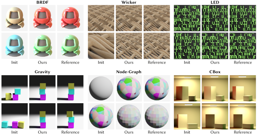
Figure 11. Visualizations of instances of our tasks. We visualize the initial configuration in the left column of each subfigure, and our outcome and the reference in the middle and right column, respectively. For our method’s convergence behaviour on these tasks, please cf. Fig. 10.

We validate our method on a variety of tasks ranging across rendering, animation, modelling and physics, all of which are not amenable to gradient-based optimization. For detailed descriptions of all tasks, please cf. Suppl. Sec. 2.2; for task-specific visualizations please cf. Fig. 11. Additionally, we evaluate how well our method scales to higher-dimensional inverse optimization problems in Sec. 4.5.

4.4. Results

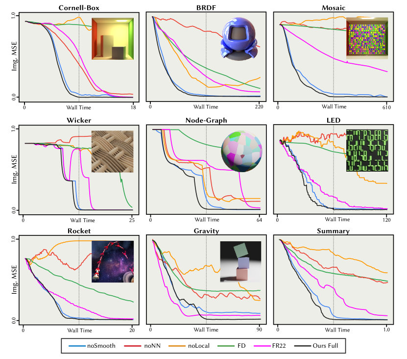
Figure 10. We show convergence plots of all methods (wall-clock time in seconds, method colors are consistent with Tab. 1) for all tasks, ranging from differentiable rendering (top row) over procedural modelling (middle row) to animation and simulation (bottom row). For all experiments, we let our method run until convergence (the dashed vertical line in each subfigure) and then allocate twice as much time for the other methods to converge. All results are reported across an ensemble of 10 independent runs for all methods. For convenience, we show a summary across all tasks in the right bottom subfigure (mean across all methods, normalized and resampled). For task-specific visualizations, please cf. Fig. 11.

We display the results of all methods listed in Tab. 1 in Fig. 10, with one subfigure per task, and show a quantitative analysis in the right part of Tab. 1. We group the results into rendering (Cornell Box, Brdf, Mosaic), modelling (Wicker, Node-Graph, Led) and animation (Rocket, Gravity), which correspond to the three rightmost columns in Tab. 1 and the rows in Fig. 10, respectively.

From the convergence plots in Fig. 10, it becomes evident that NoLocal works in select cases, but often struggles to find the correct solution, especially where the domain is higher-dimensional (e.g., Mosaic), as a uniform random sampling of the parameter space introduces substantial variance in the gradient estimates. Similarly, NoNN is challenged in higher-dimensional cases and does not converge reliably, which we attribute to the reduced expressiveness of the quadratic potential. However, this shows that for simple tasks (e.g., Cornell-Box), the proxy does not need to be overly complicated. Finite Differences (FD) works well and makes steady progress towards the target, but unfortunately does not scale well to higher dimensions, as a $d$-dimensional problem requires $2d$ function evaluations for a single gradient step (cf. the wall-time plots in Fig. 10). FR22 works reliably on all tasks, but often converges slower than our method. Surprisingly, we find that ablating the inner smoothing operation in NoSmooth only slightly impedes performance (ca. 2x), which we partly attribute to the implicit smoothing introduced by the surrogate fit.

In almost all cases, Ours works best and faithfully recovers the true parameters. The overhead of our method compared to its competitors is small: for smoothing, it suffices to slightly perturb the current state, i.e., no additional evaluation of $f$ is required. The NN query is very efficient as it can be parallelized on the GPU, and the surrogates are relatively shallow (for implementation details cf. Suppl. Sec. 1), providing Ours with the best quality-speed relation, as is evident from the right bottom subfigure in Fig. 10, where we show the (normalized and re-sampled) mean performance of all methods.

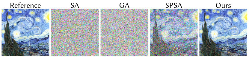
Figure 5. We show an equal-sample comparison (i.e., the same budget of function evaluations) for the task of optimizing a $256\times 256\times 3$ texture.

4.5. Higher Dimensions

We here evaluate our method on higher-dimensional inverse rendering problems and compare against the established derivative-free optimizers genetic algorithms (GA) [Holland, 1973], simulated annealing (SA) [Kirkpatrick et al., 1983] and simultaneous perturbation stochastic approximation (SPSA) [Spall, 1992]. Due to the high dimensionality of these experiments, we found it necessary to increase the surrogate capacity and the gradient batchsize (for implementation details, please cf. Suppl. Sec. 1).

Texture First, we optimize the $256\times 256$ RGB pixels of a texture (cf. Fig. 5), a relatively simple task with a smooth cost landscape and no correlation between the optimization variables. Our surrogate gradients lead to a successful optimization outcome, while the derivative-free optimizers GA and SA fail to converge due to the high problem dimensionality. SPSA achieves better results but requires more time to converge. To increase the correlation between the optimization variables, we repeat a similar task in Suppl. Fig. 2, where we use our method to optimize the weights of a multi-layered perceptron (MLP) such that it encodes digits from the MNIST [LeCun, 1998] dataset. The results are similar: our method has already converged, while SPSA makes progress but requires more function evaluations, and GA, SA and FR22 do not converge at all.

Mesh Next, we optimize the 3D position of $2,562$ vertices of a triangle mesh, as in Nicolet et al. [2021], to match a reference (cf. Fig. 9). This problem is already much harder, as the vertices are interlinked and the loss landscape exhibits discontinuities due to the rasterization process. On this task, both GA and SA fail to converge (not shown in Fig. 9), and SPSA does not find a correct solution either, whereas our approach again drives the optimization correctly to the reference.

Spline Generation Finally, we use our method to train a generative model on a non-differentiable task. Here, we use our surrogate gradients to train a variational autoencoder (VAE) [Kingma and Welling, 2013] that encodes digits from the MNIST [LeCun, 1998] dataset and outputs the support points of a spline curve, which are then rendered with a non-differentiable spline renderer. As in all tasks, we operate in image space only, so we cannot simply backpropagate through the spline renderer, but must query our surrogate for gradients.

This again is a very high-dimensional and interlinked problem, as all optimization variables (the NN weights) directly influence the spline’s final support points. For details on the training and model architecture, please cf. Suppl. Sec. 2.2.1. In Fig. 6, we sample the latent space of our model. We render the generated spline in different styles, which can easily be applied in post-processing. To our knowledge, this is the first generative model that is trained on a non-differentiable task, which again highlights the generality of our proposed approach, ZeroGrads, and gives rise to an exciting avenue of future research.

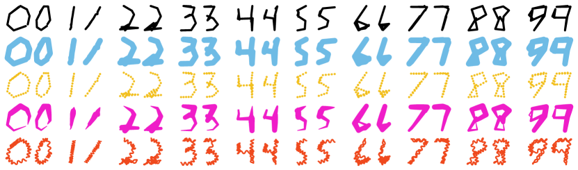
Figure 6. We sample the latent space of our trained VAE and show a variety of style transformations (rows), enabled by the spline formulation, on two digits per MNIST class. The first row displays the output of the spline renderer on which the surrogate operates.

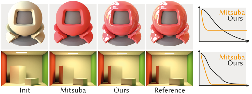
Figure 7. Comparison with Mitsuba 3 [Jakob et al., 2022] on the BRDF and Cornell-Box tasks, top and bottom row, respectively. Note that the incorrect IOR in the top row is due to Mitsuba not yet implementing this feature instead of failing during optimization (cf. Sec. 4.6).

4.6. Comparison to specific solutions

There exist many specialized solutions that enable gradient computation in graphics, and a full study of all is beyond the scope of this work. We compare qualitatively to two of these methods, rendering (Fig. 7) and procedural modelling (Fig. 8), where the common theme is that our neural surrogates are capable of optimizing their specific problems as well, and sometimes even go beyond. In Fig. 7, top row, we show that we can optimize a material’s index of refraction (IOR), a feature for which backpropagation through detached sampling has not yet been implemented in Mitsuba. As our method only needs a forward-model, we can simply combine Mitsuba’s forward path tracer with our surrogate gradients and thus are able to optimize the IOR as well. In Fig. 8, we optimize a node graph towards the target patterns, using a mixture of VGG and MSE loss, which nicely shows our surrogate’s flexibility w.r.t. to the objective $f$ . Moreover, our method also works in extreme parameter ranges, as is evident from the bottom row in Fig. 8, where the pre-trained proxy from Hu et al. [2022a] breaks due to the parameter value being out of the range it encountered during training. In summary, although our method might sometimes come at the expense of higher compute or variance (e.g., compared to Mitsuba in Fig. 7), the strength of our approach lies in its generality, i.e., in that it can be applied to arbitrary forward graphic models.

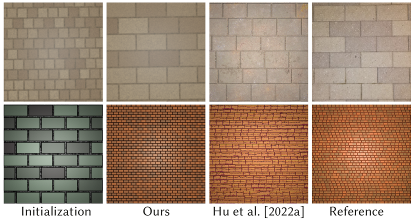
Figure 8. Comparison between Ours and Hu et al. [2022a] (results and reference taken from their publication). In the lower row, their pre-trained brick generator fails, as the parameter lies outside the training domain.

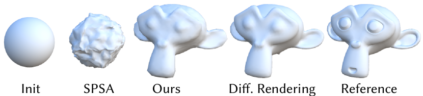
Figure 9. Starting from a tesselated sphere (left), we optimize the 3D positions of a triangle mesh with $2,562$ vertices. SPSA implements [Spall, 1992], “Diff. Rendering” uses the analytical gradients from Nicolet et al. [2021].

5. Conclusion

We have proposed ZeroGrads, a method for practical computation of surrogate gradients in non-differentiable black-box pipelines, as are found across many Graphics domains, ranging from rendering over modelling to animation. Our key ideas are the smoothing of the loss landscape, a local approximation thereof by a NN, and a low-variance estimator based on sparse, local sampling. We have favourably compared to several ablations and published alternatives and shown results for a wide variety of tasks. Additionally, we have shown our surrogate gradients to scale to high dimensionality, where traditional gradient-free optimization algorithms often do not converge. In future work, more specific estimators could help reduce the variance even further. Also, the interplay of the inner surrogate loss and outer optimizer could be explored further, e.g., by using the surrogate to also adapt the outer learning rate.

Most of the things that enable our approach are known in the optimization community that routinely uses proxies and surrogates. Yet, these ideas are rarely used in graphics, where specific solutions were developed and rarely compared against what the optimization literature offers. Our work combines graphic-specific features (e.g., MC-estimating the gradient, sampling the objective through simply rendering) and graphics-inspired improvements (such as variance reduction through importance sampling) to match requirements of graphics with general optimization.

Zero Grads Ever Given: Supplemental Materials

This supplementary contains additional information on our surrogate implementation and hyperparameter settings (Sec. 1), rendering setups (Sec. 2.1), and detailed descriptions of the tasks we solve and their respective setups (Sec. 2.2).

1. Implementation Details

We implement all our experiments in PyTorch [Paszke et al., 2017]. The proxy powering our surrogate is implemented as a MLP and activated by a leaky ReLU. We randomly initialize our Neural Proxy for each optimization run (via the standard PyTorch initialization, for the quadratic proxy, we choose the identity matrix) and optimize its weights alongside the parameter with a separate Adam optimizer. We perform three update steps on the surrogate parameters $\phi$ per optimization iteration in order to improve the surrogate’s fit to the sampled data. This is simple autodiff-driven GD and hence very fast. Note that no new data is sampled between these update steps, they merely serve to improve the surrogate fit and do not increase the required computational budget. For all gradient updates, we use the Adam optimizer with standard parameters and learning rates as specified in Tab. 2. We normalize the network’s inputs to [0,1]. For the lower-dimensional tasks ($n_{\textrm{dim}}$ ¡ 50), it suffices to use 3 hidden layers with 64 neurons each, whereas for the higher-dimensional tasks Mosaic, Mesh, Spline Generation and Texture, we found that we needed to increase the surrogate’s capacity to 8 layers à 128 neurons and additionally use positional encoding to increase the frequencies that the network can encode.

1.1. Hyperparameters

Our method comes with two hyperparameters: the number of samples $N$ we use to estimate our surrogate’s gradient with (cf. Alg.2 in the main text), and the spread of the locality kernel $\lambda$ , which will influence how far these samples are spaced out around the current parameter $\theta$ .

We specify the number of samples $N$ we use for estimating the surrogate’s gradients in Tab. 2. For the lower-dimensional tasks, it suffices to use $N=2$, whereas for the higher-dimensional tasks, the noise and higher variance from this rough gradient estimate impede convergence and thus require higher sample counts. We would like to emphasize that those are still far lower than what competing methods use, e.g., 2$n_{\textrm{dim}}$ for FD or $m\,\times\,n_{\textrm{dim}},m\gg 2$, for directional Gaussian smoothing (DGS) [Zhang et al., 2020]. Our method also benefits from more samples in the lower-dimensional regime, but these come at the cost of increase compute, which is why we tried to achieve a minimal number to keep the overhead low. We detail the remaining hyperparameters and experiment settings in Tab. 2, where $\sigma_{o}$ denotes the spread of the locality kernel $\lambda$ . As a rule of thumb, we recommend setting $\sigma_{o}$ to 0.33 on normalized domains and fine-tune from there, if necessary. For higher-dimensional, interlinked problems, we have found a more fine-granular sampling to be necessary and use $\sigma_{o}=0.025$. We use 15% of the locality spread as the spread of the smoothing kernel $\kappa$ .

Table 2. Our hyperparameters $\sigma_{o}$ and $N$ , as well as the experiment settings for the different tasks, sorted by dimensionality in ascending order. MPL is short for matplotlib.

	$\sigma_{o}$	$N$	$n_{\textrm{dim}}$	LR $\theta$	LR $\phi$	Renderer
Wicker	0.33	2	3	$1\!\times\!10^{-3}$	$1\!\times\!10^{-3}$	Blender
BRDF	0.33	2	4	$1\!\times\!10^{-3}$	$1\!\times\!10^{-3}$	Mitsuba
CBox	0.10	2	4	$5\!\times\!10^{-4}$	$1\!\times\!10^{-3}$	Mitsuba
Gravity	0.20	2	5	$1\!\times\!10^{-3}$	$1\!\times\!10^{-3}$	Blender
Rocket	0.33	2	10	$1\!\times\!10^{-3}$	$5\!\times\!10^{-4}$	MPL
NodeGr.	0.20	2	24	$1\!\times\!10^{-3}$	$1\!\times\!10^{-3}$	Blender
LED	0.33	2	336	$1\!\times\!10^{-3}$	$1\!\times\!10^{-3}$	Blender
Mosaic	0.025	16	320	$5\!\times\!10^{-4}$	$1\!\times\!10^{-3}$	Blender
Mesh	0.025	20	$7,686$	$2\!\times\!10^{-3}$	$1\!\times\!10^{-4}$	NVDiff.
Spline Gen.	0.025	20	$8,764$	$1\!\times\!10^{-4}$	$1\!\times\!10^{-4}$	MPL
Texture	0.025	20	$196,608$	$1\!\times\!10^{-5}$	$1\!\times\!10^{-4}$	MPL

2. Tasks

This section provides information on the task setup, problems, goals and rendering architectures used.

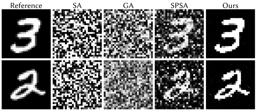
Figure 12. We show an equal-sample comparison for the task of optimizing the $35,152$ weights of a MLP such that it encodes digits from the MNIST [LeCun, 1998] dataset and compare against simulated annealing (SA), genetic algorithms (GA) and SPSA. For details, cf. Sec. 2.2.1.

2.1. Rendering

To render the images for the tasks Mosaic, Wicker, LED, NodeGraph and Gravity, we interface our method with Blender via an efficient socket-based local TCP network, which enables us to make use of Blender’s rendering engines and the embedded physics solver. All images we set to render noise-free under either Eevee or Cycles, with 16 to 128 samples and denoising activated. For the tasks BRDF and Cornell-Box, and the comparisons with Mitsuba, we use Mitsuba 3 [Jakob et al., 2022] with the path-replay backpropagation integrator at 16spp. For the Mesh task, we use NVDiffRast [Laine et al., 2020] with standard hyperparameters. For the remaining tasks Rocket, Spline Generation and Texture, we use a custom matplotlib-based renderer [Hunter, 2007]. Note that none of this interfacing is necessary for our method to work, but pure convenience for rapid prototyping and reducing I/O times from and to disk. Most importantly, we do not propagate any gradient information through the rendering process, even if this were possible, e.g., when using a differentiable renderer. One could alternatively render an image, save it to disk, manually load it and perform a gradient update step – this would yield the same results, but be arguably less convenient.

2.2. Task Descriptions

2.2.1. Higher Dimensions

We here show the optimization of higher-dimensional tasks from inverse rendering. While some of these could in theory also be solved via established, specialized methods (e.g., [Jakob et al., 2022; Nicolet et al., 2021; Holl et al., 2020]), they show that our method scales well to higher dimensional problems and reinforce our argument of general applicability.

All comparisons to the following optimization algorithms are performed under the same budget of function evaluations. For the comparisons with GA, we use the publicly available Python package geneticalgorithm [Solgi, 2020]. For SA [Xiang et al., 2013], we use the scipy library [Virtanen et al., 2020]. For SPSA [Spall, 1992], we use the publicly available spsa package [Nguyen, 2022]. Note that, while we use standard hyperparameters for the other packages, we here adapted the SPSA perturbation radius to the sampling radius used by our method in order to enable a fair comparison (the default value of 2.0 is too large for many of our problems, e.g., for the delicate task of network training).

Texture For the Texture task, we use our method to optimize the $256$ pixels of an image texture, leading to a $256\!\times\!256\!\times\!3=196,608$ optimization problem. We randomly initialize the texels from $\mathcal{N}(0.5,0.05)$, i.e., they are drawn from a Normal distribution with mean 0.5, corresponding to a grey value. As is common, we additionally employ a whitening transform during optimization [Nimier-David et al., 2019].

In Fig. 12, we show an MLP-extension of this task to address the concern that optimization variables are not sufficiently interlinked with each other. To this end, we train a MLP to replicate randomly sampled digits from the MNIST [LeCun, 1998] dataset. The MLP has two ReLU-activated hidden layers of 32 neurons and a final layer with 784 neurons that is activated by a Sigmoid, leading to a total of $35,152$ network weights and hence to a $35,152$ -dimensional optimization problem. The weights are initialized via the standard formula $\mathcal{U}(-k,k)$, where $k$ is the reciprocal of the layer’s input features [Paszke et al., 2017]. We show results in Fig. 12 and conclude that our findings from the main text apply to this setting as well: GA and SA fail to converge, and SPSA is not yet converged when our method has already found a good solution.

Mesh For the Mesh task, we optimize the vertices of a triangle mesh such that the renderings of the mesh match those of a reference shape. Our source mesh has $2,562$ vertices whose 3D positions we optimize, leading to a highly interlinked $7,686$ -dimensional problem. We follow the approach in [Nicolet et al., 2021] and use their smooth formulation, the AdamUniform optimizer and the Laplacian regularization, thereby nicely showing that our surrogate successfully learns to replicate the regularized loss landscape. For fairness, all competitors operate in this parametrization. Following [Nicolet et al., 2021], the source shape is initialized as a tessellated sphere and rendered from 13 different viewpoints under environment illumination using NVDiffRast [Laine et al., 2020] – however, without backpropagating their gradient information; all gradients employed in the optimization are produced by our surrogate.

Spline Generation For the Spline Generation task, we train a generative model, a VAE[Kingma and Welling, 2013], to replicate digits from the MNIST dataset in a spline representation. Our VAE consists of an encoder-MLP with roughly 40k neurons, and a decoder-MLP with $8,764$ neurons. To stabilize training, we use a pre-trained encoder that serves as feature extractor and projects the MNIST images into the latent space, from where we learn a generative decoder that predicts the horizontal and vertical translation of $10$ spline support points. Subsequently, we fit a spline through these predicted support points with a (matplotlib-based) non-differentiable renderer and learn our surrogate on the reconstructed splines’ image-space MSE, regularized by the VAE’s Kullback-Leibler divergence (KLD) (weighting factor $0.1$). Descending along the surrogate gradients then produces the weights for a generative decoder that can be sampled to generate new MNIST digits. Again, we initialize all stateful components with the standard formula $\mathcal{U}(-k,k)$, where $k$ is the reciprocal of a layer’s input features [Paszke et al., 2017].

2.2.2. Differentiable Rendering

Discontinuities in rendering arise from the visibility function that appears inside the integral. In that case, the gradient of the integral cannot be computed as the integral of the gradient. Typical solutions include re-parametrization or edge-sampling for path tracing [Loubet et al., 2019; Li et al., 2018] or replacing step functions with soft counterparts in rasterization [Petersen et al., 2022; Liu et al., 2019] and use framework-specific implementations.

Cornell-Box A classic scenario from differentiable rendering. We optimize the light’s horizontal and vertical translation and the axial rotation of both boxes. The discontinuities arise from visibility changes at the silhouette edges of the moving box and light.

Mosaic In this task, we simultaneously optimize the vertical rotation of 320 cubes to match a reference, leading to a 320-dimensional problem. Again, the discontinuities arise for pixels at the silhouette edges, that change their color discontinuously with the occluding cube’s rotation.

BRDF Here, we optimize the material properties (RGB reflectance and IOR) of a material test-ball illuminated under environment illumination. Optimizing properties of ideal specular objects, such as their IOR, often is not possible, even with modern differentiable path tracers [Jakob et al., 2022]. As our method does not rely on custom implementations, we can optimize these values nevertheless.

2.2.3. Modelling

Procedural modelling mainly uses nodes from two categories, filtering nodes (that are differentiable by construction) and generator nodes, that operate on discrete parameters, such as a brick texture generator. Node relations often are highly non-linear due to complex material graphs and their interplay with other pipeline parameters. Typical solutions include [Hu et al., 2022a; Guerrero et al., 2022; Shi et al., 2020; Hu et al., 2022b] and either involve lengthy, framework-specific pre-training, or rely on the existence of differentiable material libraries.

We show additional results on inverse material editing in Fig. 13, where, given a target image, we optimize the parameters of a procedural nodegraph that creates said appearance. For this task, our surrogate learns on a mixture of MSE and VGG error, as is common in inverse material optimization.

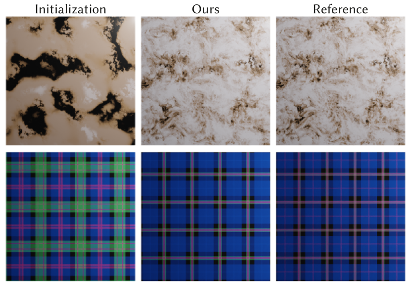
Figure 13. Our method can be used for inverse material editing in non-differentiable frameworks. Here we optimize four parameters (per row) of a node graph in order to change the final appearance towards a reference

Wicker A procedural modelling scenario where we simultaneously optimize the parameters of a node graph that creates a woven wicker material. We optimize the number of horizontal and vertical stakes and the number of repetitions across the unit plane.

LED An image synthesis scenario, where, given a target setting, we optimize each LED panel in a digital display to either be on or off. The display consists of 12 panels, each with 28 elements, leading to a 336-dimensional binary problem.

Node-Graph In this task, we directly optimize the connectivity of a set of nodes in a material graph - a mixture of a combinatorical and procedural modelling problem. We encode all possible edges for a given set of nodes in a connection matrix and optimize the matrix entries. If an entry rounds to 1, the corresponding edge is inserted into the node graph, else removed. We optimize the matrix entries of a graph with 8 nodes (several inputs and outputs each, 24 valid connections and matrix entries) to produce a rendering that matches a reference image. Some graph edges constrain each other, e.g., when a shader node already is connected, a new connection will not result in an updated image, making this an even more inter-linked problem.

2.2.4. Animation

Accurate animation relies on physical models and solves differential equations to compute a character’s behaviour or movement for a given time. Oftentimes, the forward model of such an animation is inherently discontinuous (for instance, due to collisions). At the same time, the underlying physics solver is not differentiable for the same reason rendering is not: the trajectory of an object is the solution of an ordinary differential equation (ODE), which is an integral approximated by discrete sampling locations (the time steps). If the integrand (in our case, the point in time where a force starts acting) is discontinuous, Leibniz’ rule tells us that it is not valid to differentiate the integral to get a gradient estimate.

Rocket A physical simulation where we optimize the discrete event time (i.e., the integrand is discontinuous) at which a rocket’s engine must be turned off in order to reach a certain target point. We simultaneously optimize 10 rockets flying in parallel. As the forward model is solved with a finite number of time steps, a small change does not necessarily translate to a different outcome, leading to zero gradients almost everywhere.

Gravity This task runs a physics solver to infer the collision behaviour of three cubes that are dropped onto each other. If optimized correctly, the cubes will form a tower after being dropped. We optimize the two upper cubes’ initial translation and their coefficients of restitution, the “bounciness”, which we provide as the input to the solver, thereby showing that our method can be applied to differentiate through arbitrary applications.