SuppREFERENCES
Continuous and Atlas-free Analysis of Brain Structural Connectivity
Abstract
Brain structural networks are often represented as discrete adjacency matrices with elements summarizing the connectivity between pairs of regions of interest (ROIs). These ROIs are typically determined a-priori using a brain atlas. The choice of atlas is often arbitrary and can lead to a loss of important connectivity information at the sub-ROI level. This work introduces an atlas-free framework that overcomes these issues by modeling brain connectivity using smooth random functions. In particular, we assume that the observed pattern of white matter fiber tract endpoints is driven by a latent random function defined over a product manifold domain. To facilitate statistical analysis of these high dimensional functional data objects, we develop a novel algorithm to construct a data-driven reduced-rank function space that offers a desirable trade-off between computational complexity and flexibility. Using real data from the Human Connectome Project, we show that our method outperforms state-of-the-art approaches that use the traditional atlas-based structural connectivity representation on a variety of connectivity analysis tasks. We further demonstrate how our method can be used to detect localized regions and connectivity patterns associated with group differences.
Keywords: point process, functional data analysis, structural connectivity, neuroimaging
1 Introduction
The structural connectivity (SC) of the human brain refers to the pattern of anatomical connections between different brain regions formed by white matter nerve fibers, enabling communication and information transfer essential for brain function and cognition. There is great interest in understanding the variability of this connectivity (Durante et al., 2017; Wang et al., 2019), both in relation to human traits such as cognition and personality (Zhang et al., 2019; Wang et al., 2021; Arroyo et al., 2021), and in the context of mental disorder and neurodegenerative disease (Fornito et al., 2013; Park and Friston, 2013). The most common way of representing the SC data is via a discrete network based model. In this formulation, the connectivity data is represented as a symmetric adjacency matrix , where denotes the number of disjoint regions of interest (ROIs) on the brain surface. These ROIs are determined using some predefined surface parcellation known as a brain atlas (Desikan et al., 2006; Destrieux et al., 2010). The matrix element quantifies the strength of connectivity between ROIs and , and is computed using some function of the number of connections between these respective regions. A variety of statistical procedures have been developed for the joint analysis of brain networks under this representation, see Chung et al. (2021) for a contemporary overview.
The reliance on the pre-specification of an atlas in the discrete ROI-based analysis framework is problematic for at least two major reasons. First, there is no consensus as to which atlas is best for brain connectivity analysis, and therefore the selection for a given application is somewhat ad-hoc. Analyses can be sensitive to the choice of atlas (Zalesky et al., 2010), resulting in different conclusions for different parcellation schemes of the same data. Second, this approach can introduce information loss, since fine-grained connectivity information on the sub-ROI level is aggregated in the construction of the adjacency matrix. One way to mitigate these drawbacks is to increase the number of ROIs in the parcellation. This trend can be observed in more recent atlases, e.g., Glasser et al. (2016) with regions and Schaefer et al. (2018) with regions. However, increasing the number of ROIs introduces additional challenges in data analysis. The dimension of the network grows on the order of , rendering statistical modeling and inference very challenging for even moderately large .
A collection of recent works (Gutman et al., 2014; Moyer et al., 2017; Cole et al., 2021; Mansour et al., 2022) aims to address these problems by transitioning from the discrete, ROI based representation of brain connectivity to a fully continuous model. Specifically, let and denote the left and right white surfaces of the brain. The white surface, denoted as , refers to the interface between the cortical grey matter and white matter regions. Figure 1 shows an image of the structural connectome of a randomly selected Human Connectome Project (HCP) (Glasser et al., 2013) subject embedded within the white surface of the brain. The endpoints of the white matter streamlines (colored curves) are points on . Under the continuous model, the spatial pattern of these points is assumed to be related to an unobserved continuous function on , which governs the strength of connectivity between any pair of points on . This unobserved intensity function is referred to as the continuous (structural) connectivity, a notion first formalized in Moyer et al. (2017).
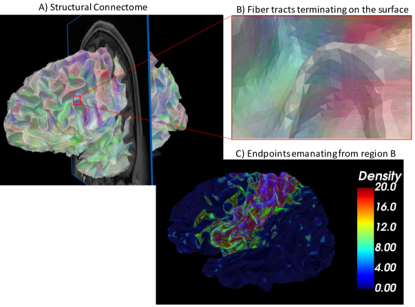
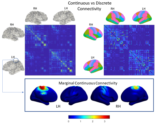
Crucially, the continuous model of connectivity does not depend on an atlas and therefore avoids the previously outlined issues which plague traditional discrete network-based approaches. Moreover, the continuous framework enables the capture of ultra-high resolution connectivity information, offering a more precise and detailed representation. For instance, the top left image in Figure 2 shows the continuous connectivity of a randomly selected HCP subject evaluated over all pairs of points in a dense grid on . Compared to the corresponding discrete atlas-based connectivity matrix shown in the top right of Figure 2, the continuous representation reveals richer and more complex patterns in the connectome.
Despite the outlined advantages, the continuous approach presents additional challenges compared to the atlas-based method that have so far limited its widespread adoption. Specifically, any computation or storage requires some form of discretization of the continuous model. The current approaches discretize the continuous connectome by forming point-wise estimates over all pairs of points in a high-resolution mesh grid on . For even moderately large grids, this generates enormous matrices, resulting in major computational hurdles for anything beyond simple subject-level analysis. Given this context, we make the following major contributions to advance the statistical analysis of continuous connectivity data:
-
1.
We extend the existing individual-level continuous connectivity framework (Gutman et al., 2014; Moyer et al., 2017; Cole et al., 2021; Mansour et al., 2022) to a population-level framework by considering the subject-level continuous connectivity as a realization of a latent random intensity function that governs the observed white matter streamline endpoints through a doubly stochastic point process model. Under our functional data model, we show how to perform canonical multi-subject statistical analysis tasks and propose a testing procedure to identify local subnetwork differences between groups.
-
2.
We develop a novel methodology and estimation algorithm to construct a data-adaptive reduced-rank function space for efficiently representing and analyzing the continuous connectivity. Such methodological development is required, as existing functional data analysis (FDA) approaches to point-process modeling have mainly been concerned with the 1-D case (Bouzas et al., 2006; Wu et al., 2013; Panaretos and Zemel, 2016; Wrobel et al., 2019) and have relied heavily on the spectral decomposition of the covariance function of the latent intensity process. This is problematic in our case due to the curse of dimensionality. The covariance function is a constrained functional object over an 8-dimensional manifold domain, making direct estimation of this object, and hence the existing approaches, computationally infeasible.
-
3.
Using a large brain imaging dataset from the HCP, we demonstrate the superiority of the continuous framework over the popular discrete framework for understanding the relationship between brain connectivity and behavioral traits.
While some initial findings of this study were previously presented in a brief conference paper by Consagra et al. (2022), the current paper significantly expands and enhances that work, introducing several innovative contributions. We offer a more detailed account of the methodological framework, which includes an explanation of the construction of the reduced-rank representation space and a detailed derivation of the estimation algorithm. In response to a crucial problem in brain network analysis, a new subsection addresses the identification of brain regions with distinct interconnections across groups, including theoretical results that describe key properties of the proposed inference procedure. Furthermore, we include a new and extensive simulation study that examines aspects such as convergence and computational complexity of the proposed estimation algorithm and statistical power/type I error of the hypothesis testing procedure. We also significantly bolster the real data analysis by adding new comparisons, demonstrating the superiority of our method compared to several state-of-the-art competitors. This comprehensive exposition enables a broader and deeper exploration of the ideas first introduced in the conference paper.
2 Structural Connectivity Data
In this section, we introduce the HCP dataset and outline the image processing procedure used to extract the structural connectivity data.
2.1 Human Connectome Project
In this work, we consider a sample of 437 female subjects from the HCP young adult cohort (https://db.humanconnectome.org). In addition to multimodal imaging data, associated with each subject are a set of measurements related to various cognitive, physical, socioeconomic and psychiatric factors, or traits. Many of these traits are defined and measured using tests from the NIH Toolbox for Assessment of Neurological and Behavioral Function (Gershon et al., 2013), though some additional tests for measuring cognitive and emotional processing were also performed. To understand the association between brain structural connectivity and human traits, we collected 175 traits spanning eight categories: cognition, motor, substance use, psychiatry, sense, emotion, personality and health.
2.2 Data Description, Image Acquisition and Processing
Diffusion magnetic resonance imaging (dMRI) measures the local anisotropy of water molecule diffusion to infer white matter microstructure. Specifically, the local geometry of the white matter induces an anisotropy in the local water molecule diffusion, with water tending to diffuse faster along the direction of the underlying neural fiber tracts. Diffusion MRI exploits this relationship and collects measurements of spatially localized diffusion signals along many different directions, called b-vectors, to obtain a 3-dimensional picture of diffusion at each location (voxel) on a regular grid over the brain volume. Smooth local models of diffusion are fit to these measurements, e.g. the diffusion tensor (Basser et al., 1994) or the orientation distribution function (ODF) (Tuch, 2004), and are subsequently used to trace out the large-scale white matter fibers using a process called tractography (Basser et al., 2000).
For each subject, we use both the dMRI and the structural T1-weighted images, the latter of which provides images with high contrast between white and grey matter regions and is therefore useful for estimating the white surface. The full imaging acquisition protocol as well as the minimal preprocessing pipeline applied to the dMRI data are given in Glasser et al. (2013), which includes susceptibility induced distortion correction and motion correction using FSL (Smith et al., 2004). The cortical white surfaces (left) and (right) were estimated from the T1 image using Freesurfer and their geometry represented using a surface triangulation with vertices. To estimate the SC, we first estimate the local models of diffusion from the dMRI data using the approach from Tournier et al. (2007) and then apply the surface enhanced tractography (SET) algorithm (St-Onge et al., 2018) to ensure the ending points of streamlines are on .
For the joint analysis of imaging data from multiple subjects, an additional source of unwanted variability comes from misalignment due to different shapes and sizes of the brain. To alleviate this issue, we parameterize each of the white surfaces using spherical coordinates via the surface inflation techniques from Fischl et al. (1999), and then apply a warping function estimated from aligning geometric features on the surface in Freesurfer to bring the white matter streamline endpoints to a common template space. The final surface endpoint connectivity data consists of counts of connections between pairs of points, which presents challenges in terms of data storage. To alleviate the disk space burden, we downsampled the registered surfaces to a resolution of vertices using a procedure that minimizes the local metric distortion (Cole et al., 2021). It’s important to note that this downsampling was purely for storage convenience, and that the proposed method is scalable to analyze data at much higher resolutions (see Supplemental Section S4.3 for an example).
3 Statistical Framework for Continuous Connectivity
In this section, we outline our structural connectivity data generating model and describe a kernel density estimator for single subject point-wise estimation.
3.1 Modeling Continuous Connectivity using Doubly Stochastic Point Processes
For a single subject, let denote the endpoints of streamlines connecting cortical white surfaces (see Figure 1). Since () is homeomorphic to , we parameterize it using spherical coordinates. Let be the image of on under the homeomorphism; we define , and with some abuse of notation we let , and hence . For a single subject, we can model the streamline endpoints as a realization of an underlying point process on with an unknown integrable intensity function defined as follows. For any two measurable regions and , denote as the counting process of the number of streamlines ending in . Then satisfies
| (1) |
In this work, we are interested in the analysis of a random sample of the structural connectivity data from subjects: . Modeling the replicated point processes with a single deterministic intensity function is likely insufficient to properly accommodate the population variability in connectivity patterns. Hence, it is reasonable to assume that the intensity function governing is itself a realization of an underlying random process, which we denote as . That is, conditional on , the first order moment of the point set satisfies Equation (1) with intensity function .
Denote as the space of symmetric functions over , i.e., for , and . We assume that has an associated measure such that i) the mean function , ii) the process has finite second order moment , iii) the covariance function is mean-square integrable and iv) is integrable almost surely. Under these conditions, is associated with a random density function, denoted . Define as a distribution on with finite moments modeling the total number of streamlines. is related to the seeding procedure in fiber tracking (Girard et al., 2014; Ambrosen et al., 2020), e.g., with more seeds, more streamlines will be observed. Conditional on and , we assume that the ’th subject’s observed streamline endpoints and that and are independent (Wu et al., 2013).
3.2 Subject-Level Estimate of Continuous Connectivity
Under the model described in Section 3.1, conditional on , we can form a pointwise estimate (and hence ) by local density estimation. In this work, we use the augmented symmetrized product heat kernel first proposed in Moyer et al. (2017) for estimating the rate function of an inhomogeneous Poisson process model for a single continuous connectome. Several alternative pointwise smoothers have been proposed in the connectomics literature (Borovitskiy et al., 2021; Mansour et al., 2022), any of which could used instead while retaining compatibility with the remainder of our methodology. In the following, we provide an explicit formulation of chosen kernel smoother. Let be the kernel function with bandwidth defined by , where is the spherical heat kernel (Chung, 2006) trivially extended to by setting if and are not on the same copy of . A point-wise estimate of and for the -th subject is given by:
| (2) | ||||
In our real data analysis, is on the order of , and so we can expect these point-wise estimates to be reasonable. Selection of the bandwidth can be performed using the cross-validation procedure described in Moyer et al. (2017).
4 Reduced-Rank Modeling of Continuous Connectivity
Given a set of continuous connectivity objects estimated using (2), this section proposes a set of novel methods for efficient joint representation and downstream statistical analyses. Proofs of all the results in this section are provided in Section S1 of the Supplemental Materials.
4.1 Functional Principal Components Analysis
Optimal reduced-rank representation for functional data has largely focused on the eigenfunctions of the covariance function . Under the mean-square integrability assumption on , Mercer’s theorem guarantees the existence of a set of non-negative eigenvalues and associated orthonormal eigenfunctions such that By the Karhunen-Loève theorem, the random function can be represented as where are independent, mean zero random variables with . The first ’s form an optimal (according to the mean integrated squared error) rank basis for representing realizations of , making them appealing for forming parsimonious finite rank approximations. Of course, the eigenfunctions are unknown and must be estimated from the data, i.e., by functional principal components analysis (FPCA) (Ramsay, 2005). A common approach to FPCA is to form a smoothed estimate and then perform a spectral decomposition over some finite-dimensional basis system or discretization of the domain (Silverman, 1996; Yao et al., 2005). However, this approach is infeasible in the current situation due to the curse of dimensionality, as is a symmetric positive semi-definite (PSD) function defined over an -D manifold domain, i.e., . For instance, imposing a grid with vertices for , the resulting discretization of is a matrix of elements, the storage of which alone requires , exceeding the computational capabilities of most currently existing computers.
Approaches to FPCA for data on complicated non-Euclidean multidimensional domains are limited. Lila et al. (2016) use finite elements to solve the best rank optimization problem, while Chen et al. (2017) and Lynch and Chen (2018) assume a separable structure on to promote tractable estimation of the marginal eigenfunctions. The former still requires solving an optimization problem over , the space of symmetric functions on the product space of two 2-D submanifolds of , hence the curse of dimensionality is still problematic. The latter introduces assumptions that are hard to verify in practice, and can be inefficient when the true covariance is not separable (Consagra et al., 2021). Instead, we propose an alternative data-driven procedure to create a reduced-rank function space, adapted to the distribution of , that is both highly flexible and avoids the curse of dimensionality.
4.2 Data-Driven Reduced-Rank Function Spaces
We begin with defining relevant notations. Without loss of generality, assume that has been centered, i.e., we consider the zero-mean process . Denote the set of unit -norm functions, called the Hilbert sphere, . Define the symmetric separable orthogonal function set of rank as
where and is the Kronecker delta.
For any , there are an infinite number of such sets. We propose to construct a adapted to the distribution of utilizing a greedy learning procedure. Specifically, given a sample of independent realizations of , we iteratively construct by repeating the following steps:
| (3) | ||||
for , where is the orthogonal projection operator onto and the process is initialized with and .
We would like to characterize the theoretical performance of the resulting approximation space, , for representing the continuous connectivity . The following theorem, which was initially presented in Consagra et al. (2022), bounds the asymptotic mean representation error of the low-rank space constructed from the greedy updates in (3) as a function of .
Theorem 1 (Consagra et al. (2022)).
In general, , so is not the optimal rank space for representing realizations of . However, offers a desirable trade-off between flexibility and computational complexity. In regard to the latter, notice that (3) requires solving an optimization problem over , while estimating the eigenfunctions requires an optimization problem over . This simplification is critical in practice, as optimization for functions directly in squares the number of unknown parameters that need to be estimated, resulting in enormous computational difficulties due to the high dimensionality of the marginal space . The flexibility of is demonstrated in Theorem 1, which establishes both asymptotic completeness and error bounds as a function of the rank.
4.3 Statistical Analysis of Reduced-Rank Continuous Connectivity
We can approximate any function in as a linear combination of basis functions in , thereby mapping the infinite dimensional continuous connectivity to a low-dimensional vector consisting of the coefficients of the basis expansion. As such, any continuous connectivity can be identified with a -dimensional Euclidean vector , with . Owing to the orthonormality of the basis functions in , the mapping is an isometry between and , where is the standard Euclidean metric. Therefore, we can properly embed the continuous connectivity into a -dimensional Euclidean vector space and utilize a multitude of existing tools from multivariate statistics for analysis of . For the remainder of this section, we discuss how to perform several canonical tasks of interest in computational neuroscience under our continuous connectivity data representation.
Trait Prediction: It is often desirable to use the structural connectivity to predict some trait of interest. This can be accommodated under our framework simply by using the embedding vectors as features in an appropriate predictive model.
Global Hypothesis Testing: Another important application is the assessment of global differences in structural connectivity between two groups. Given two samples of continuous connectivity: and , we are interested in testing , where , and denotes the group membership. Using the continuous connectivity embedding, this testing problem is translated into a two-group test on the coefficients v.s. . A non-parametric test to assess whether and are independent samples from the same distribution can be performed using the Maximum Mean Discrepancy (MMD) test statistic (Gretton et al., 2012).
Identifying Local Subnetwork Differences Between Groups: In addition to testing global connectivity difference, it is often of interest to identify where this difference manifests in the brain. In atlas-based approaches, this problem corresponds to the identification of brain subnetworks related to phenotypic traits of interest, which is a significant area of interest in modern structural connectome analysis (Chung et al., 2021). Analogously, under the continuous connectivity framework, we want to identify regions of the domain where the continuous connectivity is different between groups. This is known as a local inference problem in the FDA literature. One common approach to local inference is to represent the functional data using some basis system with local support, e.g., splines or wavelets, and then test differences on the coefficients of the expansion (Pini and Vantini, 2016). The local support property of the basis is critical as it allows the effects of the coefficients to be localized on the domain. To perform local inference for continuous connectivity, we need to construct locally supported . Therefore, we augment our basis learning procedure to include an optional constraint to promote basis with sparse support (more details are presented in Section 5).
Let , with again being the group label. The following theorem illustrates how we can link hypothesis tests on coefficient differences to the identification of subnetworks that differ between groups.
Theorem 2.
Define a collection of testing problems on the coefficients
| (4) |
Denote the index set , and define
and . A non-empty implies the following point-wise condition:
The set covers brain regions where some . Since the group labels are exchangeable under , the set of tests in Equation (4) used to construct can be performed using simple permutations and the resulting p-values corrected using Holm (1979) to control the family-wise error rate (FWER) at a pre-specified level . Denote to be the subnetwork cover constructed using the proposed testing scheme and define the false coverage probability (FCP) as follows:
| (5) |
The FCP quantifies the probability that a non-empty is formed, but it does not cover any significantly different edges. The following theorem characterizes the control of the FCP under the proposed testing procedure:
Theorem 3.
The proposed testing procedure controls the false coverage proportion at level , that is, FCP.
5 Estimation and Implementation Details
In this section, we derive an alternating optimization scheme to estimate the reduced-rank function space in (3) from the observed data and discuss associated implementation details and hyperparamter selection.
5.1 Deriving the Optimization Problem
Using the orthogonal constraint for elements in , the -th greedy search of in (3) can be equivalently formulated as:
| (6) | ||||
| s.t. |
Unfortunately, problem (6) is intractable due to the infinite-dimensional search space . In what follows, we derive a discrete approximation of problem (6) that facilities efficient computation by the algorithm proposed in Section 5.2.
For tractable computation of the inner product, we impose a dense mesh grid on . Let be the vertices on the marginal grid. Note that since is a union of two 2-spheres, are points on and are points on . For subject , denote the high-resolution symmetric continuous connectivity matrix: , where contains elements . The inner product in (6) can now be approximated as
| (7) |
where is the Frobenius inner product, are the vectors of evaluations of on , , with
| (8) |
and is the mean of the ’s, see Supplemental Section S3 for more details.
We now handle the infinite dimensional search space of through basis expansion. As is a union of two 2-spheres, we can trivially extend any complete basis system for , denoted , to , since . Denoting the -dimensional truncation (where indexes the two spheres in ), is approximated as
| (9) |
where the are the vectors of coefficients with respect to the basis . Hence, an element in can be represented as with basis functions , where . In theory, can be taken as any complete basis system for . In practice, we use spherical splines of degree 1, due to their appealing properties (see Supplemental Materials Section S2 for more discussion.)
In applications, it may be desirable to incorporate some constraints on the learned basis functions . For example, we want to promote smoothness in the to ameliorate the effect of discretization and/or estimate locally supported to facilitate the local inference procedure discussed in Section 4.3. Smoothness can be achieved through a regularization term that penalizes the candidate solution’s “roughness”, measured using the integrated quadratic variation: . Owing to the local support of the spherical spline basis functions, locally supported can be achieved by encouraging sparsity in the ’s. In particular, our estimation procedure incorporates an optional constraint set: , where is a tuning parameter controlling the level of localization of the basis functions.
Define to be the matrix of evaluations of over and denote the matrix of inner products . Define the block matrices
After incorporating the smoothness and local support constraint, the final formulation of (6) is given by
| (10) | ||||
| s.t. |
where are hyperparameters used to control the smoothness and local support size, respectively, and encodes after basis expansion (see the Supplemental Materials Section S2.2 for more details). Efficient algorithms exist for evaluating spherical splines, computing their directional derivatives as well as performing integration (Schumaker, 2015), hence the matrices and can be constructed cheaply.
5.2 Algorithm
Denote as the -dimensional semi-symmetric tensor obtained from a mode-3 stacking of the . The computational grid can be made arbitrarily dense, rendering an enormously high dimensional “functional tensor” object. This prohibits a standard tensor decomposition applied to and necessitates the development of our efficient algorithm discussed below.
The optimization problem (10) is a constrained maximization of a degree 4 polynomial with variables and thus is NP-hard (Hou and So, 2014). To derive a computationally tractable algorithm, we first notice that by combing Equations (8) and (9), we have that
| (11) |
Using approximation (11) and introducing the associated auxiliary variable , (10) can be equivalently defined as
| (12) | ||||
| s.t. | ||||
We apply an alternating optimization (AO) scheme to (12), iteratively maximizing given and vice versa. A data-reduction transformation based on the singular value decomposition is utilized in order to avoid computations that scale with the number of grid points (the dimension of ). Define the block matrices
and define , which is the transformed residual of for the ’th subject. By the properties of the Frobenius inner product, we have . Crucially, this identity can be used in problem (12) to avoid the computational burden of storing and computing with matrices of dimension .
Define the -dimensional tensor to be the mode-3 stacking of the . Then, by definition of the -mode tensor-matrix multiplication (denoted ), . Under the AO scheme, the update for the block variable at the iteration is given by
| (13) | ||||
where
| (14) |
and the ’s are from the previous selections. For , the update at the iteration is given in closed form by
| (15) |
For a detailed derivation of (13) and (15), see Section S3 of the Supplementary Materials.
If no sparsity constraint is employed, (13) reduces to finding the leading generalized eigenvector of a symmetric matrix. Since is symmetric and positive definite, this problem has a unique solution. Since (15) is trivially unique, the AO scheme of Algorithm 1 is guaranteed to converge to a stationary point of the objective by the existence and uniqueness property (Bezdek and Hathaway, 2003).
Alternatively, with the sparsity constraint active, (13) is recognized as a sparse generalized eigenvalue problem (SGEP), for which several recent methods could be applied to obtain a solution (Yuan and Zhang, 2011; Tan et al., 2018; Jung et al., 2019; Cai et al., 2021). To establish existence and uniqueness of a SGEP, additional assumptions on the problem structure are required (Cai et al., 2021), and thus we cannot typically guarantee the convergence of the resulting AO scheme. In experiments not reported, we found such convergence issues to be problematic in the very sparse (small ) regime, which corresponds to learning basis functions to detect highly localized effects. Therefore, in the interest of both computational speed and algorthmic stability, we employ an alternative two-stage procedure, in which we first obtain the non-sparsity constrained rank-1 updated and then keep only the largest elements in absolute magnitude. This “single iteration thresholding” corresponds to running a single iteration of the truncated power method from Yuan and Zhang (2011) to sparsify the final estimate. Though somewhat ad-hoc, this method was found to be faster and more stable than iterative solving of the SGEP, while also allowing a fast and simple way to select (discussed in Section 5.3). Automatic hyperparameter selection for iterative sparse reconstructions often employ an adaptive BIC-like criteria (Allen, 2012) which, while theoretically satisfying, we found to further exacerbate issues when embedded into the AO-algorithm updates.
Algorithm 1 provides pseudocode for the proposed AO scheme. Notice that the only computation that scales with the number of grid points is the transformation of the functional tensor into the tensor , which happens only once during the initialization of the procedure. Since typically , this results in an enormous savings in computation when compared to an alternative approach of performing tensor decomposition directly on . Initializations for and are obtained using the leading left singular vectors of the mode-1 and mode-3 matricization of , see Supplementary Materials Section S3 for justification.
5.3 Hyperparameter Selection
Smoothness and Sparsity: Algorithm 1 requires specifying the penalty parameters (dictating the degree of smoothness of the solution), and (determining the size of the support of ). In practice, can be selected through cross-validation on the rank-1 approximation. In our real data analysis, we found small values were preferable, likely due to the fact that the functional data has already been smoothed via KDE over a dense grid. The local support parameter can be used if locally supported basis functions are desirable, e.g., for identifying local subnetworks that are different between groups, and can be tuned according to the desired sparsity level. If automatic sparsity parameter selection is desired, notice that we may equivalently formulate the problem as finding a numerical threshold below which is set to zero. To determine , we propose to first apply univariate convex clustering to the elements of , select the cluster with centroid closest to 0, and set to be the absolute maximum over the zero-cluster elements. Similar clustering-based approaches have been used to remove estimates of small non-zero values in the high-dimensional sparse regression literature (Wu et al., 2019).
Rank Selection: It is also important to select both the marginal ranks and the global rank . The global rank can be selected using a threshold criterion on the proportion of variance explained, estimated using the transformed tensor by . Similarly, selecting the marginal ranks can be accomplished using a threshold criterion on , where is obtained from the SVD of basis evaluation matrices for a given . This quantity can be considered as an estimate of the proportion of variance explained by .
Spherical Triangulation: The optimization problem (12) is also dependent on the underlying spherical triangulation, denoted , used to define the spherical spline basis. We use a simple pruning heuristic to design , independently for each copy of , such that the local density of basis functions is aligned to the spatial distribution of . See the Supplemental Materials Section S2.3 for details.
6 Simulation Study
In this section, we study several important aspects of our proposed procedure using simulated data. Specifically, the convergence of the proposed reduced-rank function space in and for both the in-sample error (residual) and the generalization error is considered in Section 6.1, Section 6.2 assesses the computational performance of Algorithm 1, and Section 6.3 evaluates the local inference task presented in Section 4.3 on a simulated two-group testing problem. All experiments were performed using MATLAB/2020 on a Linux OS with a 2.4 GHz Intel Xeon CPU E5-2695 and 32GB of RAM.
6.1 Reconstruction Error Analysis
We simulate continuous connectivity according to: where , for and is the linear spherical spline basis formed by the Delaunay triangulation of vertices. To generate the , we independently sampled . The random coefficients were drawn independently from . The true rank was fixed to . The were evaluated at all pairs of points in the grid over discussed in Section 2.
We study the connectivity reconstruction error as a function of for training sample sizes . For each sample size, in addition to the training data, we independently sampled ’s to serve as a test set for estimating the generalization error of , for constructed from the training set. For each setting, 100 replicated experiments were performed and the mean integrated square error (MSE) of the reconstructed connectivity was estimated for both training and testing data. We used the marginal spline basis system for approximation and fixed a small roughness penalty parameter. The sparsity constraint was not active.
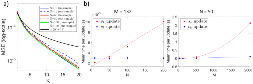
Figure 3a shows the MSE as a function of for different choices of . As increases, we observe the in-sample (training) and out-sample (testing) error curves converge to one another. The black curve is , in accord with the asymptotic error bound for the global optimum derived in Theorem 1, with constant multiple defined by averaging the errors computed for the rank 1 case. We see that for all and , on average, the errors obey the theory. Recall that the convergence of the proposed AO procedure is to a stationary point, which may not be the global solution. These simulation results indicate that the proposed AO procedure can construct solutions that exhibit the established convergence properties.
6.2 Computational Performance
We now investigate the computational performance of the rank-1 updates in Algorithm 1, which require iteratively solving (15) and (13). We use the same generative model for the connectivity as Section 6.1 and consider all combinations of sample sizes and marginal ranks . For each configuration, Algorithm 1 was run 10 times, and the mean per-update computational time was recorded along with the number of iterations required for convergence. Convergence was assessed by computing the relative change in the objective function between iterations of the inner loop in Algorithm 1, terminating when a sufficiently small value () was reached. The median number of iterations to convergence was , with the minimum and maximum being and , respectively, indicating that our algorithm converges quickly under a variety of settings.
Figure 3b displays the average computational time per update of both and . For updating , the computational time has an approximately linear relationship with the sample size (left panel) and an approximately quadratic relationship with spline rank (right panel). This is predicted by the theoretical complexity analysis: update (15) can be computed at a computational cost of . Updating is quite fast, on the order of seconds or less, for all the settings considered.
6.3 Two Group Continuous Sub-network Detection
In this section, we explore our method in the context of detecting local differences between two groups. Define two populations of functional data using the generative model:
where is a population specific effect for the group and is a common random field. Specifically,
with the symmetrized heat-kernel discussed in Section 3.2 with bandwidth centered at , where are sampled uniformly on . The random effect sizes are simulated according to , where
and is varied to simulate different signal sizes. The field is defined using the random sum of symmetric separable functions as outlined in Section 6.1, with the one change being the basis functions are determined according to: , for and is the Hadamard product, which is independently sampled to introduce sparsity. This set-up simulates the situation in which the difference between groups is confined within a small subset of connections. Our task is to be able to reliably identify the differential connections within a highly localized region.
We study the statistical power of our method under a variety of effect (signal) and sample sizes, and , respecitvely. Algorithm 1 is used to estimate with locally supported elements , where the sparsity level is automatically selected using the clustering approach discussed in Section 5.3. Local inference is performed using the testing procedure outlined in Section 4.3, controlling for FCP at the level. For each simulation setting, we consider 100 Monte-Carlo (MC) replications.
To quantify the detection performance, we computed the MC-average of the point-wise empirical coverage proportion (CP) and the empirical false coverage proportion (FCP), which can be defined here as
respectively, where denotes continuous subnetwork cover formed using the ’th Monte-Carlo dataset, and . To assess the specificity, we compute the empirical proportion of domain coverage (DC):
which measures the average size of the ’s relative to the total area of (). For a baseline comparison, we use permutations to test edgewise mean differences along with Benjamini and Hochberg (1995) correction to control FDR . We also compare our method to the popular Network-based statistic (NBS) (Zalesky et al., 2010) approach to identify significant sub-networks. We use the python implementation of NBS from the brainconn package.
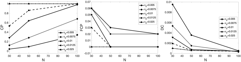
The top left panel of Figure 4 plots the estimated coverage proportion of our procedure as a function of for each considered. The statistical power, as quantified by the coverage proportion (CP), increases with and decreases for smaller effect size , as expected. The results displayed in the middle plot of Figure 4 show that the testing procedure controls the FCP at the 0.05 level for most scenarios studied, except for the low signal, low sample () cases, where the FPCs are only slightly above at 0.06. The FCP decreases with increasing sample size for all signal sizes considered. The right plot of Figure 4 shows the domain coverage (DC) as a function of . The subnetwork cover tends to shrink (becoming more precise) with increasing . Coupling this result with the positive relationship between coverage proportion and sample size indicates that our inference procedure displays desirable large sample behavior, generating increasingly tight subnetwork covers that cover the true simulated significant edge with high probability.
Edgewise testing with FDR correction resulted in no significant discoveries for all cases considered. This is not unexpected, as the number of tests is , rendering independent edgewise testing infeasible. For NBS, we could not run the entire MC study due to exceedingly long computational time (a single run with and took days). Our partial results show that even in this high-signal, large sample size setting, NBS could not identify significant connections. The observed computational bottleneck is not unexpected, as inference using the NBS algorithm comes at a computational cost of ( is the number of permutations), and thus scales poorly with the grid size. In comparison, the cost of local inference using our method is driven by the iterative updates (13) and (15), which are crucially independent of , with only trivial additional computational expenditure for permutations on the coefficients of the ’s.
7 Real Data Applications
In this section, we showcase our reduced-rank continuous connectivity representation framework—referred to here as CC—by applying the three main statistical procedures outlined in Section 4.3 to the HCP structural connectivity data discussed in Section 2. We used the computation grid on with , as outlined in Section 2. To form from the streamline endpoints of subject at all points on , the KDE bandwidth was set to be in Equation (2), in accordance with the experiments in Cole et al. (2021). For all models considered in this section, we used a spherical spline basis with , selected using an threshold on the criteria described in Section 5.3. The roughness penalty parameter was selected to be . The sparsity constraint was not active in the analysis in Sections 7.1 and 7.2, while in the analysis in Section 7.3 we selected using the automated clustering approach discussed in Section 5.3.
7.1 CC Reproducibility Analysis
Given the numerous uncertainties in the brain imaging pipeline, it is crucial to evaluate the reproducibility of any neuroimaging analysis method. Details regarding the evaluations of our method’s reproducibility are available in Section S4.2 of the Supplemental Material. Overall, our method exhibits excellent reproducibility across both scans (i.e., same subjects scanned in two separate sessions) and mesh sizes (i.e., the same subjects connectivity rendered at both 80k and 5k grid points).
7.2 Relating Brain Networks to Traits
We compare the embeddings produced by our continuous approach to those constructed from atlas-based networks using several state-of-the-art joint network embedding methods, namely, Tensor-Network PCA (TN-PCA) (Zhang et al., 2019), Multiple Random Dot-Product Graph model (MRDPG) (Nielsen and Witten, 2018) and Multiple Adjacency Spectral Embedding method (MASE) (Arroyo et al., 2021), on both hypothesis testing and prediction tasks. As a baseline, we also consider the approach of using the off-diagonal elements of the connectome matrices directly (OffDiag). For evaluation, we used the sample of 437 female HCP subjects and their corresponding traits.
Streamline count-based connectome matrices were formed from each subject’s tractography result using both the Desikan (with 68 cortical parcels) and Destriex (with 148 cortical parcels) atlases. MRDPG and MASE require a binary adjacency matrix representation of the connectivity, which was obtained by thresholding the count-based connectome matrices, while TN-PCA was applied directly to the count matrices. To facilitate fair comparison, embedding dimensions were used for all methods, except MRDPG applied to the Desikan atlas, since this method requires , and hence we let . The K-dimensional embeddings were used as representations of the SC in subsequent analysis tasks.
7.2.1 Hypothesis Testing
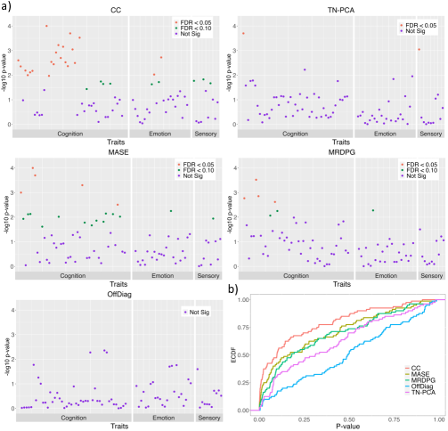
We first compare the power of the embeddings produced by different methods for identifying group differences. The groups are defined as follows: for each of the 80 measured traits in the categories cognition, emotion, and sensory, two groups were created by selecting the top 100 and bottom 100 of the 437 HCP females, in terms of their measured trait score. For each trait, we use the MMD test (Gretton et al., 2012) to test the null hypothesis that the groups of embedding vectors were drawn from the same distribution. The corresponding p-values were computed using 10,000 Monte-Carlo resampling iterations and corrected for false discovery rate (FDR) control using Benjamini and Hochberg (1995).
The five panels in Figure 5a show the p-value results for different embedding methods. The discrete network-based analysis was performed using the Destriex atlas. The y-axis gives the negative log transformed (raw) p-values and the colors indicate significant discoveries under a couple FDR control levels. With a threshold of , the embeddings produced by our method are able to identify 22 significant discoveries, compared to 7 or less for the competitors. In Figure 5b, we see that the empirical CDF of the p-values for our method has the largest departure from uniformity, the distribution expected under the null hypothesis of no difference.
Figure S2 in Supplemental Section S4.1 shows the same analysis for the network-based approaches using the Desikan atlas. The results show both fewer, and perhaps more saliently, different discoveries than using the Destriex atlas, illustrating the sensitivity of the discrete approaches to the choice of atlas. Not only does our continuous framework produce uniformly more powerful embeddings by modeling the SC data at much higher resolutions, but also the atlas-independence reduces the contingency of the reported results.
7.2.2 Trait Prediction
We now compare the performance of the different methods for the task of predicting various trait measurements from the SC. Many of the trait measurements in the HCP are under the same category (e.g., fluid intelligence, executive function and emotion recognition) and can be highly correlated with one another. Therefore, we constructed a set of composite measures using principal component analysis (PCA). Specifically, we first grouped these measurements, discarding any that were binary or categorical. The categories considered were: fluid intelligence, processing speed, self-regulation and impulse control, sustained attention, executive function, psychiatric, taste, emotional recognition, anger and hostility and finally BMI and weight. A PCA was performed for each category and the first PCs that explain of the variance were selected. Each subject’s measurements were then projected onto each of the principal directions to get PC scores, which were used as outcomes for the trait prediction task. In all, there were 31 of these.
The embeddings were used as features in a LASSO regression model for the various outcomes of interest. For each outcome of interest, we performed 100 random 80-20 train-test splits of the data. The LASSO regularization parameter was selected with cross-validation using the training data. The trained model was then applied to the test set and the Pearson correlation () between the predicted and observed values was recorded. Any outcome whose predictions were not deemed significantly associated (random train-test split average ) with any of the embedding frameworks was discarded from the analysis. In all, 15 out of the original 31 outcomes met this criterion.
Table 1 records the Pearson correlation averaged over the random train-test splits for the significant outcomes for each method. The outcomes are labeled with the convention assessment-PC number. The discrete networks used by the competitor methods were formed with the Destriex atlas. Our method outperforms all other methods for 12 out of the 15 outcomes. In several cases, the improvement is dramatic, e.g. Anger and Hostility-2, Emotion Recognition-4, Executive Function-2. This suggests potentially large gains in predictive capability when analyzing connectivity data at very high resolutions. Table S1 in Supplemental Section S4.1 gives the corresponding results for the networks formed using the Desikan atlas. Echoing the results of Section 7.2.1, for many cases, we note the predictions using the discrete network embedding techniques are highly sensitive to the choice of atlas.
| Method | |||||
|---|---|---|---|---|---|
| Outcome | CC | TN-PCA | MASE | MRDPG | OffDiag |
| Fluid Intelligence-1 | 0.1571 (0.0076) | 0.1122 (0.0069) | 0.1321 (0.0077) | 0.1235 (0.0084) | 0.1146 (0.0086) |
| Self Regulation-1 | 0.2083 (0.0083) | -0.0460 (0.0090) | 0.1280 (0.0081) | 0.1410 (0.0086) | 0.0347 (0.0089) |
| Self Regulation-3 | 0.0376 (0.0092) | 0.0464 (0.0103) | -0.0117 (0.0081) | 0.1289 (0.0097) | 0.0264 (0.0086) |
| Sustained Attention-2 | 0.1251 (0.0096) | -0.0412 (0.0084) | -0.0343 (0.0083) | -0.0031 (0.0092) | -0.0071 (0.0062) |
| Executive Function-1 | 0.1464 (0.0100) | 0.1072 (0.0079) | 0.0415 (0.0079) | 0.0881 (0.0075) | 0.1025 (0.0082) |
| Executive Function-2 | 0.1504 (0.0097) | -0.0116 (0.0092) | -0.0631 (0.0086) | 0.0521 (0.0102) | 0.0929 (0.0110) |
| Psychiatric-3 | 0.1070 (0.0088) | -0.0470 (0.0080) | -0.0107 (0.0103) | -0.0274 (0.0079) | -0.0276 (0.0093) |
| Psychiatric-6 | -0.0441 (0.0087) | 0.1277 (0.0086) | 0.1001 (0.0085) | 0.1239 (0.0096) | 0.0171 (0.0102) |
| Taste-1 | 0.1331 (0.0087) | 0.0164 (0.0087) | 0.0466 (0.0080) | 0.0214 (0.0087) | 0.0459 (0.0105) |
| Emotion Recognition-1 | 0.1023 (0.0093) | 0.0895 (0.0091) | 0.0896 (0.0080) | 0.0160 (0.0083) | 0.0378 (0.0131) |
| Emotion Recognition-2 | 0.0113 (0.0094) | 0.0489 (0.0089) | 0.1145 (0.0083) | -0.0436 (0.0092) | -0.0391 (0.0083) |
| Emotion Recognition-4 | 0.1428 (0.0084) | -0.0329 (0.0084) | -0.0659 (0.0090) | -0.0349 (0.0102) | -0.0190 (0.0051) |
| Anger and Hostility-2 | 0.2111 (0.0076) | 0.0011 (0.0096) | -0.0369 (0.0095) | -0.0379 (0.0081) | 0.0908 (0.0102) |
| Anger and Hostility-3 | 0.2062 (0.0094) | -0.0078 (0.0092) | 0.1850 (0.0090) | 0.0576 (0.0082) | -0.0057 (0.0084) |
| BMI and Weight-1 | 0.3153 (0.0076) | 0.2365 (0.0090) | 0.0866 (0.0085) | 0.1519 (0.0092) | 0.2037 (0.0089) |
7.3 Continuous Subnetwork Discovery
In this section, we illustrate how to identify connections that are different between groups using our continuous framework. In order to focus the analysis, we consider the cognitive trait impulsivity, as measured by delay discounting. Delay discounting measures the tendency for people to prefer smaller, immediate rewards over larger, but delayed rewards. It is known that steep discounting is associated with a variety of psychiatric conditions, including antisocial personality disorders, drug abuse and pathological gambling (Odum, 2011). The HCP collects several measures of delay discounting on each participant as a part of a self-regulation/impulsivity assessment. In this study we focus on one of the measures, namely, the subjective value of in 6 months. For this measure, a series of trials are performed in which the subjects are made to choose between two alternatives: in 6 months or a smaller amount today. For each trial, reward amounts are adjusted based on the subject’s choices to iteratively determine an indifference amount that identifies the participants subjective value of in 6 months. For more information on how this measurement is collected, we refer the interested reader to Estle et al. (2006).
From the sample of 437 female HCP subjects, we sub-selected and classified them to have high or low discounting, according to their subjective value of at 6 months. In particular, the subject was classified to the high discounting group if their subjective value , and to the low discounting group if it was . This resulted in a total sample size of 142: 64 in the high discounting group and 78 in the low discounting group. Locally supported basis functions () were estimated using the full set of 437 HCP female subjects, with sparsity threshold selected using the automated clustering approach outlined in Section 5.3. The local inference procedure formulated in Section 4.3 was then applied to form with using permutations.
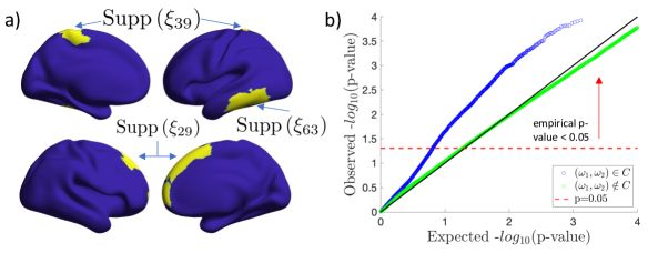
The coefficients associated with basis functions and were identified to be significantly different between high and low discounting groups. Figure 6a shows the support sets of these selected basis functions (yellow regions) plotted on the cortical surface. To validate this finding, we conducted point-wise t-tests for all connections , and plotted the empirical p-values vs. the expected p-values (under ) in Figure 6b, for both and . The skew of the -log10-transformed p-values of the former indicates the presence of sub-regions of where the continuous connectivity differs between groups.
The support sets show significant coverage of regions and connections in the prefrontal cortex. These results are strongly supported by the literature. Generally, areas in the prefrontal cortex are known to be critical for advanced decisions involving reward (Rogers et al., 1999). Particular areas covered include the right superior frontal, middle frontal and orbitofrontal cortex. Previous studies have shown delay discounting to be associated with the grey matter volume in these areas (Wang et al., 2016; Owens et al., 2017). We also notice substantial coverage in the left paracentral region, which is thought to be primarily involved with motor and somatosensory processing, though task fMRI studies have identified this region to be active when choosing immediate rewards vs. control choices in delay discounting tasks (Stanger et al., 2013). The final area of significant coverage is the rather large area on the left temporal lobe, a region which is known to be heavily involved with temporal information processing (Elias et al., 1999). Additionally, Olson et al. (2009) found strong evidence of significant alterations in white matter in this region between high and low discount groups. Recalling that the continuous subnetwork covers significant connections between any pair of points, all identified regions can be interpreted jointly in terms of possible subnetworks between them. The task fMRI literature has identified possible functional networks related to delay discounting which include areas in the prefrontal, parietal and temporal regions (Olson et al., 2009). Such networks are consistent with the coverage implied by , suggesting a possible link between the significant functional and structural networks of importance.
8 Conclusion and Future Directions
This work introduces a novel modeling framework for the analysis of structural connectivity. We define the continuous structural connectivity as a latent random function on the symmetric product space of the cortical surface that governs the distribution of white matter fiber tract endpoints. This continuous representation allows us to bypass issues that plague the traditional discrete network based approaches but also poses new challenges for computation and modeling due to the super-high dimensionalities of the data. To facilitate tractable representation and analysis, we formulate a data-adaptive reduced-rank function space that avoids the curse of dimensionality. To construct a set of basis functions that span this space, we derive a penalized optimization problem and propose a novel computationally efficient algorithm for estimation. The proposed method was applied to several critical neuroscience applications, including hypothesis testing and trait prediction. Through comparison with state-of-the-art atlas-based network analysis methods, we demonstrated the superior performance of the proposed framework in real data analysis of HCP data.
We conclude by noting several possible extensions of the proposed framework. First, a unified method that is able to estimate directly from the streamline endpoints without the need for the intermediate KDE smoothing step is desirable. Second, forming the low rank model by decomposing the variability directly in the linear space may not be ideal, as this does not explicitly respect the constraints on . There are several geometric frameworks for performing functional data modeling of random densities, e.g. Srivastava et al. (2011); Petersen and Müller (2016), but their extension to our case is non-trivial due to the complex multidimensional domain , and hence more investigation is required. Third, our method employs the Holm procedure to control the FWER when comparing random coefficients () from two subject groups to ensure the control over the FCP of the random intensity functions. While the Holm procedure ensures tight control of the FWER regardless of the dependence structure of the test statistics, this versatility may lead to over-conservativeness in practice. Exploring alternative FWER control methods, such as those assuming mild conditions on the joint distribution of test statistics (Meinshausen et al., 2011), could lead to a more powerful local inference procedure, and is therefore an important direction for future work.
Code: Implementation of our method along with code for processing the SC data has been made publicly available: https://github.com/sbci-brain/SBCI_Modeling_FPCA
References
- Allen (2012) Allen, G. (2012). Sparse higher-order principal components analysis. In AISTATS.
- Ambrosen et al. (2020) Ambrosen, K. S., S. F. Eskildsen, M. Hinne, K. Krug, H. Lundell, M. N. Schmidt, M. A. van Gerven, M. Mørup, and T. B. Dyrby (2020). Validation of structural brain connectivity networks: The impact of scanning parameters. NeuroImage 204, 116207.
- Arroyo et al. (2021) Arroyo, J., A. Athreya, J. Cape, G. Chen, C. E. Priebe, and J. T. Vogelstein (2021). Inference for multiple heterogeneous networks with a common invariant subspace. Journal of machine learning research 22(141), 1–49.
- Basser et al. (1994) Basser, P., J. Mattiello, and D. Lebihan (1994). Estimation of the effective self-diffusion tensor from the NMR spin echo. Journal of Magnetic Resonance, Series B 103, 247–254.
- Basser et al. (2000) Basser, P. J., S. Pajevic, C. Pierpaoli, J. Duda, and A. Aldroubi (2000). In vivo fiber tractography using dt-mri data. Magnetic Resonance in Medicine 44(4), 625–632.
- Benjamini and Hochberg (1995) Benjamini, Y. and Y. Hochberg (1995). Controlling the false discovery rate: A practical and powerful approach to multiple testing. Journal of the Royal Statistical Society. Series B (Methodological) 57(1), 289–300.
- Bezdek and Hathaway (2003) Bezdek, J. and R. Hathaway (2003, 12). Convergence of alternating optimization. Neural, Parallel & Scientific Computations 11, 351–368.
- Borovitskiy et al. (2021) Borovitskiy, V., I. Azangulov, A. Terenin, P. Mostowsky, M. P. Deisenroth, and N. Durrande (2021). Matern gaussian processes on graphs. In International Conference on Artificial Intelligence and Statistics. PMLR.
- Bouzas et al. (2006) Bouzas, P., M. Valderrama, A. Aguilera, and N. Ruiz-Fuentes (2006). Modelling the mean of a doubly stochastic poisson process by functional data analysis. Computational Statistics & Data Analysis 50(10), 2655–2667.
- Cai et al. (2021) Cai, Y., G. Fang, and P. Li (2021). A note on sparse generalized eigenvalue problem. In Thirty-Fifth Conference on Neural Information Processing Systems.
- Chen et al. (2017) Chen, K., P. Delicado, and H.-G. Müller (2017). Modelling function-valued stochastic processes, with applications to fertility dynamics. Journal of the Royal Statistical Society: Series B (Statistical Methodology) 79(1), 177–196.
- Chung et al. (2021) Chung, J., E. Bridgeford, J. Arroyo, B. D. Pedigo, A. Saad-Eldin, V. Gopalakrishnan, L. Xiang, C. E. Priebe, and J. T. Vogelstein (2021). Statistical connectomics. Annual Review of Statistics and Its Application 8(1), 463–492.
- Chung (2006) Chung, M. (2006). Heat kernel smoothing on unit sphere. In 3rd IEEE International Symposium on Biomedical Imaging: Nano to Macro, 2006., pp. 992–995.
- Cole et al. (2021) Cole, M., K. Murray, E. St-Onge, B. Risk, J. Zhong, G. Schifitto, M. Descoteaux, and Z. Zhang (2021). Surface-based connectivity integration: An atlas-free approach to jointly study functional and structural connectivity. Human Brain Mapping 42(11), 3481–3499.
- Consagra et al. (2022) Consagra, W., M. Cole, and Z. Zhang (2022). Analyzing brain structural connectivity as continuous random functions. arXiv: Statistics Computation.
- Consagra et al. (2021) Consagra, W., A. Venkataraman, and X. Qiu (2021). Efficient multidimensional functional data analysis using marginal product basis systems. arXiv: Statistics Methodology.
- Desikan et al. (2006) Desikan, R. S., F. Ségonne, B. Fischl, B. T. Quinn, B. C. Dickerson, D. Blacker, R. L. Buckner, A. M. Dale, R. P. Maguire, B. T. Hyman, M. S. Albert, and R. J. Killiany (2006). An automated labeling system for subdividing the human cerebral cortex on mri scans into gyral based regions of interest. NeuroImage 31(3), 968–980.
- Destrieux et al. (2010) Destrieux, C., B. Fischl, A. Dale, and E. Halgren (2010). Automatic parcellation of human cortical gyri and sulci using standard anatomical nomenclature. NeuroImage 53(1), 1–15.
- Durante et al. (2017) Durante, D., D. B. Dunson, and J. T. Vogelstein (2017). Nonparametric bayes modeling of populations of networks. Journal of the American Statistical Association 112(520), 1516–1530.
- Elias et al. (1999) Elias, L. J., M. Bulman-Fleming, and I. McManus (1999). Visual temporal asymmetries are related to asymmetries in linguistic perception. Neuropsychologia 37(11), 1243–1249.
- Estle et al. (2006) Estle, S. J., L. Green, J. Myerson, and D. D. Holt (2006). Differential effects of amount on temporal and probability discounting of gains and losses. Memory & Cognition 34(4), 914–928.
- Fischl et al. (1999) Fischl, B., M. I. Sereno, and A. M. Dale (1999). Cortical surface-based analysis: Ii: inflation, flattening, and a surface-based coordinate system. Neuroimage 9(2), 195–207.
- Fornito et al. (2013) Fornito, A., A. Zalesky, and M. Breakspear (2013). Graph analysis of the human connectome: Promise, progress, and pitfalls. NeuroImage 80, 426–444. Mapping the Connectome.
- Gershon et al. (2013) Gershon, R. C., M. V. Wagster, H. C. Hendrie, N. A. Fox, K. F. Cook, and C. J. Nowinski (2013). Nih toolbox for assessment of neurological and behavioral function. Neurology 80(11 Supplement 3), S2–S6.
- Girard et al. (2014) Girard, G., K. Whittingstall, R. Deriche, and M. Descoteaux (2014). Towards quantitative connectivity analysis: reducing tractography biases. Neuroimage 98, 266–278.
- Glasser et al. (2016) Glasser, M. F., T. S. Coalson, E. C. Robinson, C. D. Hacker, J. Harwell, E. Yacoub, K. Ugurbil, J. Andersson, C. F. Beckmann, M. Jenkinson, et al. (2016). A multi-modal parcellation of human cerebral cortex. Nature 536(7615), 171–178.
- Glasser et al. (2013) Glasser, M. F., S. N. Sotiropoulos, J. A. Wilson, T. S. Coalson, B. Fischl, J. L. Andersson, J. Xu, S. Jbabdi, M. Webster, J. R. Polimeni, D. C. V. Essen, M. Jenkinson, and f. t. W.-M. H. Consortium (2013). The minimal preprocessing pipelines for the Human Connectome Project. NeuroImage 80, 105–124.
- Gretton et al. (2012) Gretton, A., K. M. Borgwardt, M. J. Rasch, B. Schölkopf, and A. Smola (2012). A kernel two-sample test. Journal of Machine Learning Research 13(25), 723–773.
- Gretton et al. (2012) Gretton, A., K. M. Borgwardt, M. J. Rasch, B. Schölkopf, and A. Smola (2012). A kernel two-sample test. The Journal of Machine Learning Research 13(1), 723–773.
- Gutman et al. (2014) Gutman, B., C. Leonardo, N. Jahanshad, D. Hibar, K. Eschenburg, T. Nir, J. Villalon, and P. Thompson (2014). Registering cortical surfaces based on whole-brain structural connectivity and continuous connectivity analysis. Med Image Comput Comput Assist Interv 17(3), 161–168.
- Holm (1979) Holm, S. (1979). A simple sequentially rejective multiple test procedure. Scandinavian Journal of Statistics 6(2), 65–70.
- Hou and So (2014) Hou, K. and A. M.-C. So (2014). Hardness and approximation results for lp-ball constrained homogeneous polynomial optimization problems. Mathematics of Operations Research 39(4), 1084–1108.
- Jung et al. (2019) Jung, S., J. Ahn, and Y. Jeon (2019). Penalized orthogonal iteration for sparse estimation of generalized eigenvalue problem. Journal of Computational and Graphical Statistics 28(3), 710–721.
- Lila et al. (2016) Lila, E., J. A. D. Aston, and L. M. Sangalli (2016, 12). Smooth principal component analysis over two-dimensional manifolds with an application to neuroimaging. The Annals of Applied Statistics 10(4), 1854–1879.
- Lynch and Chen (2018) Lynch, B. and K. Chen (2018, 09). A test of weak separability for multi-way functional data, with application to brain connectivity studies. Biometrika 105(4), 815–831.
- Mansour et al. (2022) Mansour, S., C. Seguin, R. E. Smith, and A. Zalesky (2022). Connectome spatial smoothing (css): Concepts, methods, and evaluation. NeuroImage 250, 118930.
- Meinshausen et al. (2011) Meinshausen, N., M. H. Maathuis, and P. Bühlmann (2011). Asymptotic optimality of the westfall-young permutation procedure for multiple testing under dependence. The Annals of Statistics 39(6), 3369–3391.
- Moyer et al. (2017) Moyer, D., B. A. Gutman, J. Faskowitz, N. Jahanshad, and P. M. Thompson (2017). Continuous representations of brain connectivity using spatial point processes. Medical Image Analysis 41, 32 – 39.
- Nielsen and Witten (2018) Nielsen, A. M. and D. Witten (2018). The multiple random dot product graph model. arXiv: Statistics Methodology.
- Odum (2011) Odum, A. L. (2011). Delay discounting: Trait variable? Behavioural Processes 87(1), 1–9. Society for the Quantitative Analyses of Behavior.
- Olson et al. (2009) Olson, E. A., P. F. Collins, C. J. Hooper, R. Muetzel, K. O. Lim, and M. Luciana (2009). White matter integrity predicts delay discounting behavior in 9- to 23-year-olds: A diffusion tensor imaging study. Journal of Cognitive Neuroscience 21(7), 1406–1421.
- Owens et al. (2017) Owens, M. M., J. C. Gray, M. T. Amlung, A. Oshri, L. H. Sweet, and J. MacKillop (2017). Neuroanatomical foundations of delayed reward discounting decision making. NeuroImage 161, 261–270.
- Panaretos and Zemel (2016) Panaretos, V. M. and Y. Zemel (2016). Amplitude and phase variation of point processes. The Annals of Statistics 44(2), 771 – 812.
- Park and Friston (2013) Park, H.-J. and K. Friston (2013). Structural and functional brain networks: From connections to cognition. Science 342(6158).
- Petersen and Müller (2016) Petersen, A. and H.-G. Müller (2016). Functional data analysis for density functions by transformation to a Hilbert space. The Annals of Statistics 44(1), 183 – 218.
- Pini and Vantini (2016) Pini, A. and S. Vantini (2016). The interval testing procedure: A general framework for inference in functional data analysis. Biometrics 72(3), 835–845.
- Ramsay (2005) Ramsay, J. (2005). Functional Data Analysis. American Cancer Society.
- Rogers et al. (1999) Rogers, R. D., A. M. Owen, H. C. Middleton, E. J. Williams, J. D. Pickard, B. J. Sahakian, and T. W. Robbins (1999, Oct). Choosing between small, likely rewards and large, unlikely rewards activates inferior and orbital prefrontal cortex. J Neurosci 19(20), 9029–9038.
- Schaefer et al. (2018) Schaefer, A., R. Kong, E. M. Gordon, T. O. Laumann, X. N. Zuo, A. J. Holmes, S. B. Eickhoff, and B. T. T. Yeo (2018, Sep). Local-Global Parcellation of the Human Cerebral Cortex from Intrinsic Functional Connectivity MRI. Cereb Cortex 28(9), 3095–3114.
- Schumaker (2015) Schumaker, L. (2015). Spline functions - computational methods. Society for Industrial and Applied Mathematics.
- Silverman (1996) Silverman, B. W. (1996). Smoothed functional principal components analysis by choice of norm. The Annals of Statistics 24(1), 1–24.
- Smith et al. (2004) Smith, S. M., M. Jenkinson, M. W. Woolrich, C. F. Beckmann, T. E. Behrens, H. Johansen-Berg, P. R. Bannister, M. De Luca, I. Drobnjak, D. E. Flitney, R. K. Niazy, J. Saunders, J. Vickers, Y. Zhang, N. De Stefano, J. M. Brady, and P. M. Matthews (2004). Advances in functional and structural mr image analysis and implementation as fsl. NeuroImage 23, S208–S219.
- Srivastava et al. (2011) Srivastava, A., E. Klassen, S. H. Joshi, and I. H. Jermyn (2011). Shape analysis of elastic curves in euclidean spaces. IEEE Transactions on Pattern Analysis and Machine Intelligence 33(7), 1415–1428.
- St-Onge et al. (2018) St-Onge, E., A. Daducci, G. Girard, and M. Descoteaux (2018). Surface-enhanced tractography. NeuroImage 169, 524–539.
- Stanger et al. (2013) Stanger, C., A. Elton, S. R. Ryan, G. A. James, A. J. Budney, and C. D. Kilts (2013). Neuroeconomics and adolescent substance abuse: Individual differences in neural networks and delay discounting. Journal of the American Academy of Child & Adolescent Psychiatry 52(7), 747–755.e6.
- Tan et al. (2018) Tan, K. M., Z. Wang, H. Liu, and T. Zhang (2018). Sparse generalized eigenvalue problem: optimal statistical rates via truncated rayleigh flow. Journal of the Royal Statistical Society: Series B (Statistical Methodology) 80(5), 1057–1086.
- Tournier et al. (2007) Tournier, J. D., F. Calamante, and A. Connelly (2007). Robust determination of the fibre orientation distribution in diffusion MRI: non-negativity constrained super-resolved spherical deconvolution. Neuroimage 35(4), 1459–1472.
- Tuch (2004) Tuch, D. S. (2004). Q‐ball imaging. Magnetic Resonance in Medicine 52, 1358–1372.
- Wang et al. (2019) Wang, L., Z. Zhang, and D. Dunson (2019). Common and individual structure of brain networks. The Annals of Applied Statistics 13(1), 85 – 112.
- Wang et al. (2016) Wang, Q., C. Chen, Y. Cai, S. Li, X. Zhao, L. Zheng, H. Zhang, J. Liu, C. Chen, and G. Xue (2016, 07). Dissociated neural substrates underlying impulsive choice and impulsive action. Neuroimage 134, 540–549.
- Wang et al. (2021) Wang, S., J. Arroyo, J. T. Vogelstein, and C. E. Priebe (2021). Joint embedding of graphs. IEEE Transactions on Pattern Analysis and Machine Intelligence 43(4), 1324–1336.
- Wrobel et al. (2019) Wrobel, J., V. Zipunnikov, J. Schrack, and J. Goldsmith (2019). Registration for exponential family functional data. Biometrics 75(1), 48–57.
- Wu et al. (2019) Wu, L., X. Qiu, Y. xiang Yuan, and H. Wu (2019). Parameter estimation and variable selection for big systems of linear ordinary differential equations: A matrix-based approach. Journal of the American Statistical Association 114(526), 657–667.
- Wu et al. (2013) Wu, S., H.-G. Müller, and Z. Zhang (2013). Functional data analysis for point processes with rare events. Statistica Sinica 23(1), 1–23.
- Yao et al. (2005) Yao, F., H.-G. Müller, and J.-L. Wang (2005). Functional linear regression analysis for longitudinal data. The Annals of Statistics, 2873–2903.
- Yuan and Zhang (2011) Yuan, X.-T. and T. Zhang (2011). Truncated power method for sparse eigenvalue problems. Journal of Machine Learning Research 14.
- Zalesky et al. (2010) Zalesky, A., A. Fornito, and E. T. Bullmore (2010). Network-based statistic: Identifying differences in brain networks. NeuroImage 53(4), 1197–1207.
- Zalesky et al. (2010) Zalesky, A., A. Fornito, I. H. Harding, L. Cocchi, M. Yücel, C. Pantelis, and E. T. Bullmore (2010). Whole-brain anatomical networks: Does the choice of nodes matter? NeuroImage 50(3), 970–983.
- Zhang et al. (2019) Zhang, Z., G. I. Allen, H. Zhu, and D. Dunson (2019). Tensor network factorizations: Relationships between brain structural connectomes and traits. NeuroImage 197, 330 – 343.
Supplementary Material
S1 Theory and Proofs
S1.1 Proof of Theorem 1
In order to proceed, we make the following assumptions related to the smoothness of .
Definition 1.
Let and . Define as the class of functions
where , for .
Assumption S1 (Eigenfunction Smoothness).
There exists some for and , such that for all .
Assumption S2 (Moment Bound).
For some , , holds with probability 1.
Assumption S3 (Tail Decay).
The function class in Definition 1 has been used in the literature for establishing error convergence rates for deterministic function approximation algorithms \citeSuppTemlyakov2003NonlinearMO,barron2008. This assumption is closely related to the smoothness of the ’s, see the Section S1.4 for more details. Assumptions S2 and S3 control the tail behavior of . Note that Assumption S3 introduces a slightly stronger condition on the decay rate of the spectrum than the one guaranteed by the mean square integrability of , i.e. , though it is satisfied for many commonly used covariance kernels.
Proof.
Notice that
where . Then
where the last inequality holds almost surely. ∎
Proof.
Denote , we have
| (S.1) | ||||
and
so
∎
Proof of Theorem 1
Proof.
Notice that we can write
| (S.2) | ||||
For clarity, denote with . We have,
| (S.3) | ||||
We have that
| (S.4) | ||||
Combining (S.4) and (S.3) gives the bound
By the definition of our greedy selection algorithm, we have that
Plugging these results into the recurrence relation (S.2), we obtain
| (S.5) | ||||
From the strong law of large numbers, , the bound in proposition S2, and the continuous mapping theorem, it follows that taking the large sample limit of (S.5) gives
| (S.6) |
almost surely. Notice that
where the first inequality comes from the fact that the norm dominates in sequence spaces and the second from Assumption S1. Hence, we have
| (S.7) |
almost surely. Hence the sequence is decreasing (in ).
We now derive the final result by induction. For clarity, denote For , it follows from Equation S.7 that . Assume that for any . Then if , clearly since it is a decreasing sequence. If , then using this fact along with the recurrence (S.6) and induction hypothesis, we have
establishing the desired result. ∎
S1.2 Proof of Theorem 2
Proof.
Assume that and take . Denote the marginal random function . Assume that for any . By the continuous mapping theorem, this implies , which in turn implies , which is a contradiction under . Hence, it must be the case that for some , which implies such that .
We now show that must be in . We proceed by contradiction. Assume . Let , then implies
which is a contradiction since for all . Hence, since , the desired result follows. ∎
S1.3 Proof of Theorem 3
Proof.
We are interested in bounding the probability
We proceed by cases. First, assume that , with for . Under the rank- approximation , this implies the point-wise condition
Furthermore, is equivalent to the condition is true . By definition of the FWER control, we have that our testing procedure satisfies:
and hence,
Now consider the case . Let and define . If , then this implies that would be constructed by false rejections, and by the assumed strong control of the FWER correction procedure
| (S.8) | ||||
Furthermore, from the definition of , we have
and from , we have
so as a result
holds using the the local support property. Coupling this with Equation S.8, it follows that for this case as well.
Now, the final case is and . Take any and define the operator . Applying the continuous mapping theorem to the point-wise equality of distribution condition in (5), we have that
which is a contradiction, hence cannot hold in this case and so . ∎
S1.4 Eigenfunction Smoothness
In this section, we provide more detail about the implications of Assumption S1. First, we note that this condition in trivially satisfied when the eigenfunctions are separable, as taking to be the collection of eigenfunctions clearly ensures for all . A sufficient, though not necessary, condition for eigenfunction separability is the covaraince function itself being separable.
The following proposition ensures that each can be represented by a countable set of separable functions.
Proposition S3.
For any , there exists at least one countable set , possibly with , such that .
Proof.
Let be a complete orthogonal basis system for . Then by definition, for , we have that , where , due to symmetry. Denote the infinite symmetric matrix
Since , it follows that and therefore determines a Hilbert–Schmidt operator and thus is compact. Then by the spectral theorem, there exists real eigenvalues and orthogonal eigenvectors such that
Hsing2015TheoreticalFO. Let , it follows that both
and
completing the proof. ∎
Let be the decomposition guaranteed by proposition S3 for eigenfunction and define such that form a complete orthogonal basis system (CONS) in . The summability condition in Assumption S1 can be written as:
We consider the upper bound given by:
| (S.9) |
Since is a CONS, we have that for all and :
and thus Equation S.9 reduces to the condition that , for some and for all .
To understand the implications of the absolute summability bound on the eigenvalues, we consider the following operator associated with each eigenfunction. As is symmetric and integrable, it defines the integral operator on : for . It is easy to show that
and thus is bounded. A straight-forward consequence of the symmetry of is that is self-adjoint. Furthermore, using the fact the is compact and thus has a countable set of eigenvalues (4.2.3 \citeSuppHsing2015TheoreticalFO), it is easy to show by definition that the eigenvalues of are . Then Assumption S1 is equivalent to the condition that all the ’s are Trace class operators with , as for bounded linear self-adjoint operators \citepSuppHsing2015TheoreticalFO.
We now consider what type of conditions on guarantees that , for all . In the context of familiar function classes, from theorem 13, ch. 30 in \citeSupplax2014functional, a sufficient condition for to be trace-class is being . Though the uniform bound does not have as simple an interpretation in terms of familiar function classes, a characterization can be formed by assuming is a composite operator of two bounded Hilbert-Schmidt operators:
Proposition S4.
Assume symmetric such that
and , then .
Proof.
Using the Cauchy–Schwarz inequality, the definition of the trace of an integral operator, and the unit measure assumption on , we have:
∎
As a final point, we note that Assumption S1 can almost certainly be weakened, e.g., by using the “interpolation spaces” between and , as was the tactic in \citeSuppbarron2008 in their work on the approximation of unknown deterministic functions. We leave an extension of our results for random functions in this more general space as a direction of future work.
S2 Marginal Basis System
S2.1 Spherical Splines
Define a spherical triangle with vertices , as the set of points in that are bounded by the great circle arcs connecting , and . A collection of spherical triangles is a spherical triangulation of , provided that the intersection between any two elements in is empty, a common vertex or a common edge and . The spherical Delaunay triangulation is the unique triangulation over a set of points such that the minimum angle in the triangulation is as large as possible.
For each spherical triangle , we can define a local coordinate system called the spherical barycentric coordinates, defined for to be the nonnegative real numbers satisfying
We can define the linear spherical Bernstein basis on as the span of the three nodal basis functions . That is, for any , there exists coefficients such that . The local basis functions defined for each spherical triangle can be “glued together” to form a piecewise continuous linear spline space over . Following \citeSupplai2007, we define
An explicit basis for can be constructed as follows: for each vertex in tessellation , let such that
It can be shown that is unique and that forms a basis for \citepSupplai2007.
The have many attractive properties. In particular, efficient algorithms exist for evaluating and computing their directional derivative using the local basis functions. Additionally, their local support property is crucial for the development of our local inference procedure, outlined in Section 4.3. For further information, see the excellent references \citepSupplai2007,schumaker2015.
S2.2 Penalty Matrix Computation
Proposition S5.
Under the basis expansion in Equation (9), the quadratic variation penalty has the representation
where is the Jacobian of .
Proof.
Since , the gradient separates as
We have
∎
Fast algorithms exist for computing the required directional derivatives to form \citepSupplai2007. The required integrals can be computed using Lebedev quadrature rules or using exact rules for the local planar triangle approximation to the spherical triangle. The latter of these is of course faster and preferable when the spherical triangles are small enough.
S2.3 Selecting the Triangulation
It is well established that the geometric properties of the spherical triangles in and the spatial distribution of vertices can heavily affect the approximation power of \citepSuppshewchuk2002. It is, therefore, important to have a procedure to construct . Considering the complex geometry of the white surface, the grid points are usually irregularly spaced over . We use a simple pruning heuristic to design , independently for each copy of , such that the local density of basis functions is aligned to the spatial distribution of . In particular, our approach consists of the following steps: i) initiate a dense set of (nearly) equispaced vertices over , ii) compute the pairwise distances between this vertex set and the grid , iii) sequentially prune vertices that have the largest minimum distance to the grid points until vertices are left, and iv) define to be the spherical Delaunay tessellation \citepSupplai2007 over this refined vertex set. This simple heuristic was observed to consistently result in better reconstruction performance than the (nearly) equispaced vertex strategy for the same . Figure S1 shows the tessellaton resulting from this pruning method that was used to define the marginal spline basis system in the real data experiments on both hemispheres along with the high-resolution grid points .
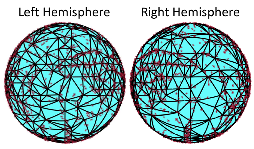
S3 Algorithm
Derivation of Approximation in Equation (7)
The approximation in Equation (7) uses the matrix element-wise inner product (e.g., ) as a discrete approximation to the continuous integral in the inner product, under the assumption that the grid points are relatively dense and reasonably spaced over . To see why this is the case, consider the following. Denote the disjoint partition formed by the spherical Voronoi tesselation of : with being the center of \citepSuppdu2003. Using Riemann sums, the inner product of functions , can be approximated as
for surface measure , as the partition becomes arbitrarily fine. Assuming that the element measures are reasonably similar to one another, i.e. , (the points are well dispersed and dense), we can make the further approximation
| (S.10) |
The desired result follows after noting that the right-hand side of Equation S.10 is proportional to the of the evaluation matrices of and on .
Derivation of Block Updates
We first state and prove two results that will be useful for our derivation.
Proposition S6.
Define the reparameterization . Then
| (S.11) |
where and .
Proof.
For clarity, in the following derivation we work mainly in the transformed parameter . For notational convenience, we define the quantities
so
Proposition S7.
Let . Then the orthogonality constraint is equivalent the condition that
where
Proof.
Note that the matrix is symmetric and positive definite and therefore defines an inner product on . The result then follows trivially from standard results in linear algebra. ∎
Using Proposition S6, we can reparamterize problem (12) as
| (S.12) | ||||
| s.t. | ||||
where the rewritten constraint follows from the element-wise definition of in Proposition S6 coupled with the definition of -mode multiplication. Noting that we have , (S.12) becomes
| s.t. | |||
Applying Proposition S7, the orthogonality constraint can be absorbed into the objective function, resulting in
| s.t. | |||
Transforming back to the original coordinates using and invoking the relaxed norm constraint,
and the updates (13) and (15) follow trivially by applying block coordinate ascent to the above.
Initialization
The block update (13) requires an initialization for and . Notice that, under the rank-1 approximation of , we have that
Then by properties of the -mode matricization,
| (S.13) |
where denotes the Kronecker product and (d) denotes the -mode matricization. Equation (S.13) indicates that, for the ’th rank-1 factor, the leading left singular vectors of and, under the transform , are a reasonable initialization for the block variables and , respectively. In practice, these can be computed efficiently using power iterations on the symmetric matrices and .
S4 Additional Results
S4.1 Brain Network and Traits
Figure S2 shows the results of the hypothesis testing task described in Section 7.2.1 and Table S1 shows the results from the prediction task from Section 7.2.2, where the discrete network-based approaches were applied to the connectomes formed via the Desikan atlas. Coupled with the results displayed in Figure 5 and Table 1, we make the following two important observations: i) our method (CC) again strongly outperforms the competitors on the Desikan atlas for most outcomes ii) the results from the competitor methods are highly variable between atlases.
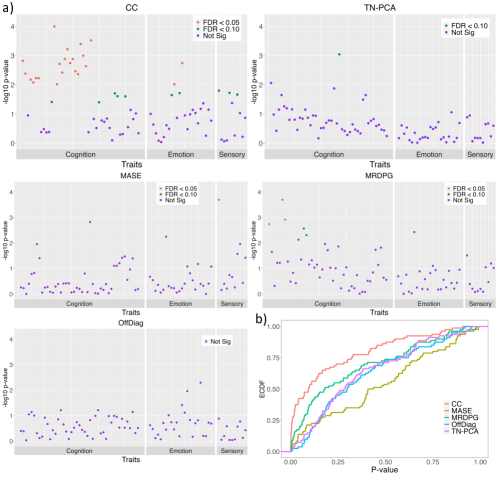
| Embedding | ||||
|---|---|---|---|---|
| Outcome | TNPCA | MASE | MRDP | OffDiag |
| Fluid Intelligence-1 | 0.1789 (0.0074) | -0.1025 (0.0090) | -0.0046 (0.0097) | 0.0898 (0.0083) |
| Self Regulation-1 | 0.0938 (0.0081) | -0.0094 (0.0088) | -0.0105 (0.0088) | 0.1586 (0.0077) |
| Self Regulation-3 | 0.1510 (0.0093) | -0.0061 (0.0094) | -0.0795 (0.0077) | -0.0244 (0.0103) |
| Sustained Attention-2 | 0.0355 (0.0088) | -0.0585 (0.0084) | -0.0825 (0.0093) | 0.0229 (0.0083) |
| Executive Function-1 | 0.0002 (0.0086) | 0.0431 (0.0091) | 0.0699 (0.0087) | 0.1086 (0.0091) |
| Executive Function-2 | -0.0459 (0.0086) | 0.0070 (0.0085) | 0.0066 (0.0083) | -0.0717 (0.0107) |
| Psychiatric-3 | 0.0508 (0.0095) | -0.0569 (0.0078) | -0.0176 (0.0094) | 0.1052 (0.0096) |
| Psychiatric-6 | -0.0315 (0.0077) | 0.1068 (0.0101) | -0.0235 (0.0093) | 0.1604 (0.0094) |
| Taste-1 | -0.0878 (0.0087) | 0.1155 (0.0082) | 0.0396 (0.0083) | -0.0054 (0.0093) |
| Emotion Recognition-1 | 0.0307 (0.0092) | 0.0938 (0.0092) | 0.0182 (0.0086) | 0.0559 (0.0085) |
| Emotion Recognition-2 | 0.0136 (0.0083) | -0.0518 (0.0071) | 0.0118 (0.0093) | 0.0775 (0.0103) |
| Emotion Recognition-4 | 0.1113 (0.0104) | -0.0594 (0.0086) | -0.0042 (0.0084) | 0.0292 (0.0108) |
| Anger and Hostility-2 | -0.0301 (0.0083) | -0.0683 (0.0086) | -0.0351 (0.0092) | 0.0574 (0.0091) |
| Anger and Hostility-3 | -0.0820 (0.0073) | 0.0400 (0.0071) | 0.1181 (0.0092) | -0.0032 (0.0091) |
| BMI and Weight-1 | 0.2082 (0.0095) | 0.0462 (0.0102) | 0.0647 (0.0088) | 0.2420 (0.0093) |
S4.2 Reproducibility Analysis
S4.2.1 Scan-Rescan Reproducibility
We are interested in studying the reproducibility of the proposed reduced-rank representation across scans. That is, we want to understand how well the reduced-rank function space, , estimated from one population, can represent the re-scanned data from the same population. For this evaluation, we utilize the HCP scan-rescan data, which consists of a subset of HCP subjects for whom two scans were collected during different sessions several months apart. This dataset contains 37 subjects and a total of 74 scans. In the absence of disease, we expect the brain organization of a healthy adult to be relatively constant over the span of several months, and therefore the HCP scan-rescan data can be considered as independent noisy samples of the same connectome, making it appealing for evaluating reproducibility. In particular, we used the scan-1 data to form estimates according to the procedure in Section 5. For several , the estimated were used to represent the scan-2 data by standard basis expansion under the least squares principle. In Figure S3a, we show the first three coefficients corresponding to for a random collection of 10 test-retest subjects. The unique markers identify multiple scans from the same individual. One can see that a within-subject clustering pattern is already present using only basis functions.
The pairwise distances between the basis expansion representations of all the scan-1 and scan-2 data were computed. Figure S3b displays the pairwise distance matrices for several different ’s. Each matrix is , giving the pairwise distances between the scans from subjects. Scans from the same subject are put next to each other, generating small blocks along the diagonal. A quantitative assessment of the reproducibility was obtained using the leave-one-out cross-validated (LOOCV) accuracy of the nearest neighbor classifier applied to the distances: for each representation , we compute , where is shorthand for the distance between scans and . The LOOCV accuracy is computed as the fraction of examples where and are two scans corresponding to the same individual. At the bottom of Figure S3b, we show the LOOCV accuracy results. With , we achieved a classification accuracy.
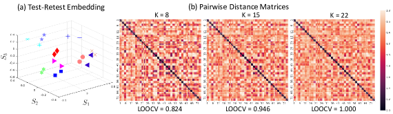
S4.3 Reproducibility Across Grid Resolutions
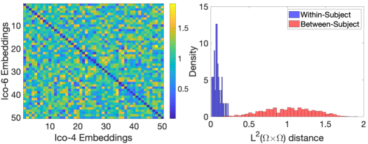
A primary advantage of the proposed methodology is its agnosticism to the grid . Hence, another form of reproducibility of interest is between grid resolutions. In other words, we are interested in how representations computed from the connectivity data of the same subject at multiple different grid resolutions compare to each other. Therefore, in this section, we compare the reproducibility of the continuous embeddings estimated from connectivity data at multiple resolutions.
Although storage considerations were the primary reason for the initial dimension reduction of the HCP connectome data from to vertices, the point-wise smoother using the heat-kernel from \citeSuppmoyer2017, i.e. Equation (2), itself can become a computational bottleneck for extremely dense grids. As discussed in Section 3.2, there are alternative estimators for the point-wise smoothed connectivity that can easily be swapped into our framework, and fast point-wise smoothing for high-dimensional connectivity data is an active area of research \citeSuppborovitskiy2021. To avoid this computational bottlekneck in this analysis, we use a simple fast alternative local smoother, defined as follows:
-
1.
Triangulate the grid points on .
-
2.
For each pair of grid points , obtain each pair of triangles which have or as a vertex. Denote these sets of triangles as and , respectively.
-
3.
For any endpoint which falls within a pair of triangles in , assign weight to be the product of the barycentric coordinates of in with respect to the and in with respect to the .
-
4.
Form as the sum of the over all endpoints.
This simple endpoint smoothing method has been used in the literature and will soon be available in the SBCI pipeline \citepSuppcole2021.
In this analysis, we use data from the Adolescent Brain Cognitive Development (ABCD) study \citepSuppcasey2018abcd. Full imaging and acquisition protocol for this data can be found in the same reference. We randomly select 50 baseline (year 1) scans and run them through the same image processing pipeline as outlined in Section 2.2, except we use the smoother defined above to form point-estimates at two resolutions, 5,124 total grid points and 81,924 total grid points, formed via an icosphere parcellation with subdivision 4 and 6, respectively. We estimate a data-driven basis from the connectivity data at both resolutions, denoted for the grid point and for the grid points, using the same model and algorithm parameters outlined in Section 7 with . We then project the representations in to the space spanned by and compute the pairwise distances between all functions.
Figure S4 (left) shows the resulting pairwise distance matrix, where the rows and columns are organized so that the same subject’s data at different resolutions appears along the diagonal. The right plot of Figure S4 shows the corresponding within subject distances, i.e. the diagonal, in blue and the between subject distances in red. We see clear separation between subjects, despite using only basis functions and forming the pointwise estimates using the rather crude estimator outlined above. This shows both that our method is scalable to extremely high dimensional grids and produces consistent and reproducible function representations between grid-size granularities.
S4.4 Comparison with Super-High Resolution Atlas-Based Method
We conducted an investigation comparing our method with high-resolution atlases using data from 300 ABCD subjects, each with two scans, one from baseline and a 1-year follow-up. Specifically, we experimented with a parcellation encompassing approximately 4,000 small triangular parcels. Raw fiber count between each pair of triangular parcels was computed as the discrete connectivity. Our findings indicate that raw high-resolution atlases significantly reduce the reproducibility of our connectivity results and are not effective predictors of cognitive traits. In particular, the atlas-based connectivity, when evaluated using dICC (analogous to ICC for quantifying reproducibility, as discussed in greater detail in \citeSuppzhang2018mapping), yields a value less than 0.55. In contrast, the CC’s dICC value is over 0.75. Similarly, CC’s predictive power for behavioral traits (e.g., picture vocabulary age-adjusted and crystallized intelligence age-adjusted) significantly surpasses that of the high-resolution atlas-based connectivity. The correlation between CC predicted picture vocabulary measures and the actual measures is 0.31 while the value for the raw high-resolution connectivity is 0.27. The values for the crystallized trait are 0.32 and 0.28, respectively.
We attribute these results to two key factors. First, the network derived from the high-resolution atlas is exceedingly sparse, making network estimation unreliable. For instance, while we typically construct about streamlines or fiber curves, an atlas with 4000 parcels can yield up to connections, and most pairs of parcels are unconnected. Second, the presence of small nodes complicates node alignment, leading to inflated variance among connections due to the node misalignment issue (nodes in classical brain network analysis are presumed to be matched). \bibliographystyleSuppchicago \bibliographySuppreferences