MapTRv2: An End-to-End Framework for Online Vectorized HD Map Construction

Abstract

High-definition (HD) map provides abundant and precise static environmental information of the driving scene, serving as a fundamental and indispensable component for planning in autonomous driving system. In this paper, we present Map TRansformer, an end-to-end framework for online vectorized HD map construction. We propose a unified permutation-equivalent modeling approach, i.e., modeling map element as a point set with a group of equivalent permutations, which accurately describes the shape of map element and stabilizes the learning process. We design a hierarchical query embedding scheme to flexibly encode structured map information and perform hierarchical bipartite matching for map element learning. To speed up convergence, we further introduce auxiliary one-to-many matching and dense supervision. The proposed method well copes with various map elements with arbitrary shapes. It runs at real-time inference speed and achieves state-of-the-art performance on both nuScenes and Argoverse2 datasets. Abundant qualitative results show stable and robust map construction quality in complex and various driving scenes. Code and more demos are available at https://github.com/hustvl/MapTR for facilitating further studies and applications.

1 Introduction

High-definition (HD) map is the high-precision map specifically designed for autonomous driving, composed of instance-level vectorized representation of map elements (pedestrian crossing, lane divider, road boundaries, centerline, etc.). HD map contains rich semantic information about road topology and traffic rules, which is essential for the navigation of self-driving vehicles.

Conventionally HD map is constructed offline using SLAM-based methods [1, 2, 3], which brings many issues: 1) complicated pipeline and high cost; 2) difficult to keep maps up-to-date; 3) misalignment with ego vehicle and high localization error (empirically, 0.4m longitudinally and 0.2m laterally).

Given these limitations, recently, online HD map construction has attracted ever-increasing interest, which constructs map around ego-vehicle at runtime with vehicle-mounted sensors and well solves the problems above.

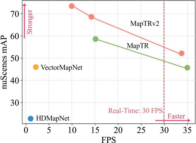
Figure 1: Speed-accuracy trade-off comparisons. The proposed MapTR/MapTRv2 framework outperforms previous state-of-the-art methods in terms of both speed (FPS) and accuracy (mAP). Compared with MapTR, MapTRv2 further improves performance by a large margin. The FPSs are measured on one NVIDIA RTX 3090.

Early works [4, 5, 6] leverage line-shape priors to perceive open-shape lanes only on the front-view image. They are restricted to single-view perception and can not cope with other map elements with arbitrary shapes. With the development of bird’s eye view (BEV) representation learning, recent works [7, 8, 9, 10] predict rasterized map by performing BEV semantic segmentation.

However, the rasterized map lacks vectorized instance-level information, such as the lane structure, which is important for the downstream tasks (e.g., motion prediction and planning). To construct the vectorized HD map, HDMapNet [11] groups pixel-wise segmentation results into vectorized instances, which requires complicated and time-consuming post-processing. VectorMapNet [12] represents each map element as a point sequence. It adopts a cascaded coarse-to-fine framework and utilizes an auto-regressive decoder to predict points sequentially, leading to long inference time and error accumulation.

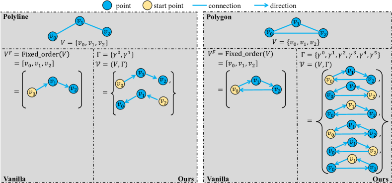
Figure 2: Illustration of permutation-equivalent shape modeling. Map elements are geometrically abstracted and discretized into polylines and polygons. MapTRv2 models each map element with $(V,\Gamma)$ (a point set $V$ and a group of equivalent permutations $\Gamma$), avoiding ambiguity and stabilizing the learning process. A special case is, if the polyline element has a specific direction (e.g., centerline), $\Gamma$ includes only one permutation.

Current online vectorized HD map construction methods are restricted by the efficiency and precision, especially in real-time scenarios. Recently, DETR [13] employs a simple and efficient encoder-decoder Transformer architecture and achieves end-to-end object detection. It is natural to ask a question: Can we design a DETR-like paradigm for efficient end-to-end vectorized HD map construction? We show that the answer is affirmative with our proposed Map TRansformer.

Different from object detection in which objects can be easily geometrically abstracted as bounding boxes, vectorized map elements have more dynamic shapes. To accurately describe map elements, we propose a novel unified modeling method. We model each map element as a point set with a group of equivalent permutations. The point set determines the position of the map element. And the permutation group includes all the possible organization sequences of the point set corresponding to the same geometrical shape, avoiding the ambiguity of shape.

Based on the permutation-equivalent modeling, we design a structured framework that takes vehicle-mounted sensor data as input and outputs vectorized HD map. We streamline the online vectorized HD map construction as a parallel regression problem. Hierarchical query embeddings are proposed to flexibly encode instance-level and point-level information. All instances and all points of instance are simultaneously predicted with a unified Transformer structure. To reduce the cost of computation and memory, we introduce decoupled self-attention for interaction among queries, i.e., respectively performing attention along the inter-ins. dimension and intra-ins. dimension.

The training pipeline is formulated as a set prediction task, where we perform hierarchical bipartite matching to assign instances and points in turn. And we supervise the geometrical shape in both point and edge levels with the proposed point-to-point loss and edge direction loss.

To speed up the convergence, we add an auxiliary one-to-many matching branch during training, which increases the ratio of positive samples. To further leverage semantic and geometric information, we introduce auxiliary foreground segmentation on both perspective view (PV) and bird’s eye view (BEV), and leverage depth supervision to guide the backbone to learn 3D geometrical information.

With all the proposed designs, we present MapTRv2, an efficient end-to-end online vectorized HD map construction method with unified modeling and architecture. MapTRv2 achieves the best performance and efficiency among existing vectorized map construction approaches on both nuScenes [14] dataset and Argoverse2 [15] dataset. In particular, on nuScenes, MapTRv2 based on ResNet18 backbone runs at real-time inference speed (33.7 FPS) on RTX 3090, $15\times$ faster than the previous state-of-the-art (SOTA) camera-based method VectorMapNet while achieving 6.3 higher mAP. With ResNet50 as the backbone, MapTRv2 achieves 68.7 mAP at 14.1 FPS, which is 22.7 mAP higher and $6\times$ faster than VectorMapNet-ResNet50, and even outperforms multi-modality VectorMapNet. When scaling up to a larger backbone VoVNetV2-99, MapTRv2 sets a new record (73.4 mAP and 9.9 FPS) with only-camera input. On Argoverse2, MapTRv2 outperforms VectorMapNet by 28.9 mAP in terms of 3D map construction with the same backbone ResNet50. As the visualization shows (Fig. 9 and Fig. 10), MapTRv2 maintains stable and robust map construction quality in complex and various driving scenes.

Our contributions can be summarized as follows:

• We propose a unified permutation-equivalent modeling approach for map elements, i.e., modeling map element as a point set with a group of equivalent permutations, which accurately describes the shape of map element and stabilizes the learning process.

• Based on the novel modeling, we present a structured end-to-end framework for efficient online vectorized HD map construction. We design a hierarchical query embedding scheme to flexibly encode instance-level and point-level information, and perform hierarchical bipartite matching for map element learning. To speed up convergence, we further introduce auxiliary one-to-many matching and auxiliary dense supervision.

• Our method is the first real-time and SOTA vectorized HD map construction approach with stable and robust performance in complex and various driving scenes.

This journal paper (MapTRv2) is an extension of a conference paper (MapTR) published at ICLR 2023 [16]. Improvements compared to the former version are as follows. First, we introduce decoupled self-attention tailored for the hierarchical query mechanism, which greatly reduces the memory consumption and brings gain. Second, we introduce auxiliary one-to-many set prediction branch to speed up the convergence. Third, we adopt auxiliary dense supervision on both perspective view and bird’s eyes view, which significantly boosts the performance. Fourth, MapTRv2 extends MapTR to modeling and learning centerline, which is important for downstream motion planning. Fifth, we provide more theoretical analysis and discussions about the proposed modules, which reveal more about the working mechanism of our framework. Finally, we extend the framework to 3D map construction (the conference version learns 2D map), and provide additional experiments on Argoverse2 dataset [15].

2 Related Work

HD Map Construction. Recently, with the development of PV-to-BEV methods [17, 18], HD map construction is formulated as a segmentation problem based on surround-view image data captured by vehicle-mounted cameras. [7, 8, 9, 10, 19, 20, 21, 22, 23, 24] generate rasterized map by performing BEV semantic segmentation. To build vectorized HD map, HDMapNet [11] groups pixel-wise semantic segmentation results with heuristic and time-consuming post-processing to generate vectorized instances. VectorMapNet [12] serves as the first end-to-end framework, which adopts a two-stage coarse-to-fine framework and utilizes auto-regressive decoder to predict points sequentially, leading to long inference time and the ambiguity about permutation. Different from VectorMapNet, our method introduces novel and unified shape modeling for map elements, solving the ambiguity and stabilizing the learning process. And we further build a structured and parallel one-stage framework with much higher efficiency. Concurrent and follow-up works of our conference version [16] focus on other promising designs of end-to-end HD map construction [25, 26, 27, 28, 29] and extend to other relative tasks [30, 31, 32, 33, 34, 35]. BeMapNet [26] adopts a unified piecewise Bezier curve to describe the geometrical shape of map elements and directly utilizes the well-established set prediction paradigm with resort to Transformer. NMP [30] introduces a neural representation of global maps that enables automatic global map updates and enhances local map inference performance. TopoNet [31] proposes a comprehensive framework to learn the connection relationship of lanes and the assignment relationship between lanes and traffic elements. PolyDiffuse [28] introduces diffusion mechanism into MapTR to further refine the results via a conditional generation procedure. MapVR [27] applies differentiable rasterization to the vectorized results produced by MapTR to incorporate precise and geometry-aware supervision. MapTRv2 extends MapTR to a more general framework. It supports centerline learning and 3D map construction. It also achieves higher accuracy and faster convergence speed.

Lane Detection. Lane detection can be viewed as a sub task of HD map construction, which focuses on detecting lane elements in the road scenes. Since most datasets of lane detection only provide single view annotations and focus on open-shape elements, related methods [36, 4, 37, 5, 38, 39, 6, 40, 41, 42, 43] are restricted to single view. LaneATT [37] utilizes an anchor-based deep lane detection model to achieve good trade-off between accuracy and efficiency. LSTR [5] adopts the Transformer architecture to directly output parameters of a lane shape model. GANet [38] formulates lane detection as a keypoint estimation and association problem and takes a bottom-up design. [39] proposes parametric Bezier curve-based method for lane detection. Instead of detecting lanes in the 2D image coordinate, [44] proposes 3D-LaneNet which performs 3D lane detection in BEV. STSU [6] represents lanes as a directed graph in BEV coordinates and adopts the curve-based Bezier method to predict lanes from the monocular camera image. Persformer [4] provides better BEV feature representation and optimizes anchor design to unify 2D and 3D lane detection simultaneously. BEV-LaneDet [36] presents a virtual camera to guarantee consistency and proposes an efficient spatial transformation pyramid module.

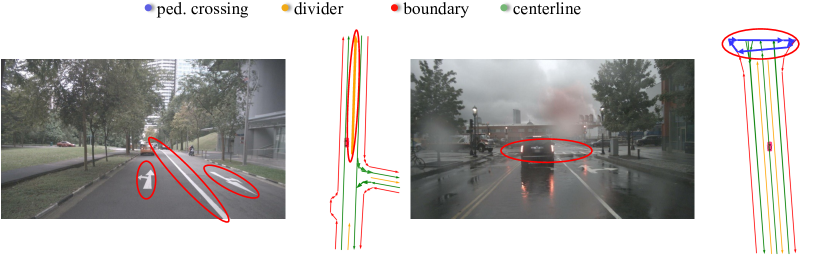
Figure 3: Typical cases for illustrating the ambiguity of map element in terms of start point and direction. Left: for polyline with unspecific direction (e.g., the lane divider between two opposite lanes), defining its direction is difficult. Both endpoints of the lane divider can be regarded as the start point and the point set can be organized in two directions. Right: for polygon (e.g., pedestrian crossing), each point of the polygon can be regarded as the start point, and the polygon can be connected in two opposite directions (counter-clockwise and clockwise). Note that some kinds of map elements (like centerline) have specific direction and have no ambiguity issue.

Contour-based 2D Instance Segmentation. Another line of related work is contour-based 2D instance segmentation [45, 46, 47, 48, 49, 50, 51, 52, 53]. These methods reformulate 2D instance segmentation as object contour prediction task, where the object contour is a closed-shape polygon, and estimate the image coordinates of the contour vertices. CurveGCN [54] utilizes Graph Convolution Networks to predict polygonal boundaries. PolarMask [46] produces the instance contour through instance center classification and dense distance regression in a polar coordinate system. Deepsnake [55] proposes a two-stage contour evolution process and designs circular convolution to exploit the features of the contour. BoundaryFormer [56] adopts advanced Transformer architecture and follows the two-stage paradigm to generate the polygon vertices based on the intermediate box results predicted by the first stage. SharpContour [45] proposes an efficient and generic contour-based boundary refinement approach to iteratively deform the contour by updating offsets in a discrete manner.

Detection Transformers. As a pioneer work, DETR [13] eliminates the need for hand-crafted components (e.g., anchor generation, ruled-based label assignment, non-maximum suppression post-processing.), and built the first fully end-to-end object detector. It represents object boxes as a set of queries and directly adopts a unified Transformer encoder-decoder architecture to perform object box detection. Due to the effectiveness and simplicity of DETR and its varieties [57, 58, 59, 60, 61, 62, 63, 64], their paradigms have been widely transferred in many complex tasks, such as 2D instance segmentation [65, 66, 67], 2D pose estimation [68, 69, 70], 3D object detection [71, 10, 72, 73]. Directly inheriting the simplicity and end-to-end manner from DETR, we propose MapTRv2 to efficiently produce high-quality vectorized HD map online.

3 Shape Modeling

MapTRv2 aims at modeling and learning the HD map in a unified manner. HD map is a collection of vectorized static map elements, including pedestrian crossing, lane divider, road boundary, centerline, etc. For structured modeling, MapTRv2 geometrically abstracts map elements as closed shape (like pedestrian crossing) and open shape (like lane divider). Through sampling points sequentially along the shape boundary, closed-shape element is discretized into polygon while open-shape element is discretized into polyline.

Preliminarily, both polygon and polyline can be represented as an ordered point set ${V}^{F}=[v_{0},v_{1},\dots,v_{N_{v}-1}]$ (see Fig. 2 (Vanilla)). $N_{v}$ denotes the number of points. However, the permutation of the point set is not explicitly defined and not unique. There exist many equivalent permutations for polygon and polyline. For example, as illustrated in Fig. 3 (a), for the lane divider (polyline) between two opposite lanes, defining its direction is difficult. Both endpoints of the lane divider can be regarded as the start point and the point set can be organized in two directions. In Fig. 3 (b), for the pedestrian crossing (polygon), the point set can be organized in two opposite directions (counter-clockwise and clockwise). And circularly changing the permutation of point set has no influence on the geometrical shape of the polygon. Imposing a fixed permutation to the point set as supervision is not rational. The imposed fixed permutation contradicts with other equivalent permutations, hampering the learning process.

To bridge this gap, MapTRv2 models each map element with $\mathcal{V}=(V,\Gamma)$. $V=\{v_{j}\}_{j=0}^{N_{v}-1}$ denotes the point set of the map element ($N_{v}$ is the number of points). $\Gamma=\{\gamma^{k}\}$ denotes a group of equivalent permutations of the point set $V$, covering all the possible organization sequences.

Specifically, for polyline element with unspecific direction (see Fig. 2 (left)), $\Gamma$ includes $2$ kinds of equivalent permutations:

$$\Gamma_{\rm{polyline}}= \{\gamma^{0},\gamma^{1}\}$$ (1)

$$= \begin{cases}\gamma^{0}(j)=j\%N_{v},\\ \gamma^{1}(j)=(N_{v}-1)-j\%N_{v}.\\ \end{cases}$$

For polyline element with specific direction (e.g., centerline), $\Gamma$ includes only one permutation: $\{\gamma^{0}\}$.

For polygon element (see Fig. 2 (right)), $\Gamma$ includes $2\times N_{v}$ kinds of equivalent permutations:

$$\Gamma_{\rm{polygon}}= \{\gamma^{0},\dots,\gamma^{2\times N_{v}-1}\}$$ (2)

$$= \begin{cases}\gamma^{0}(j)=j\%N_{v},\\ \gamma^{1}(j)=(N_{v}-1)-j\%N_{v},\\ \gamma^{2}(j)=(j+1)\%N_{v},\\ \gamma^{3}(j)=(N_{v}-1)-(j+1)\%N_{v},\\ ...\\ \gamma^{2\times N_{v}-2}(j)=(j+N_{v}-1)\%N_{v},\\ \gamma^{2\times N_{v}-1}(j)=(N_{v}-1)-(j+N_{v}-1)\%N_{v}.\end{cases}$$

By introducing the conception of equivalent permutations, MapTRv2 models map elements in a unified manner and addresses the ambiguity issue.

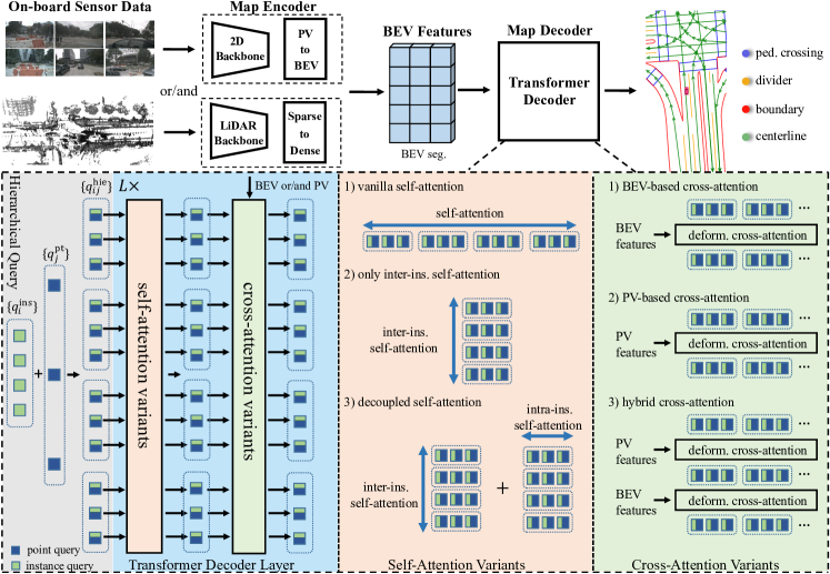
Figure 4: The overall architecture of MapTRv2. MapTRv2 adopts an encoder-decoder paradigm. The map encoder transforms sensor input to a unified BEV representation. The map decoder adopts a hierarchical query embedding scheme to explicitly encode map elements. The $L$ stacked Transformer decoder layers iteratively refine the predicted map elements. We propose several self-attention variants and cross-attention variants to efficiently update the query features. MapTRv2 is fully end-to-end. The pipeline is highly structured, compact and efficient.

4 Architecture

MapTRv2 adopts an encoder-decoder paradigm. The overall architecture is depicted in Fig. 4.

4.1 Map Encoder

The map encoder extracts features from sensor data and transforms the features into a unified feature representation, i.e., BEV representation. MapTRv2 is compatible with various vehicle-mounted sensors. Taking multi-view images $\mathcal{I}=\{I_{1},\ldots,I_{M}\}$ for example, we leverage a conventional backbone to generate multi-view feature maps $\mathcal{F}=\{F_{1},\ldots,F_{M}\}$. Then PV image features $\mathcal{F}$ are transformed to BEV features $\mathcal{B}\in\mathbb{R}^{H\times W\times C}$. We support various PV2BEV transformation methods, e.g., CVT [8], LSS [19, 21, 74, 75], Deformable Attention [10, 57], GKT [7] and IPM [76]. In MapTRv2, to explicitly exploit the depth information [74], we choose LSS-based BEVPoolv2 [77] as the default transformation method. Extending MapTRv2 to multi-modality sensor data is straightforward and trivial.

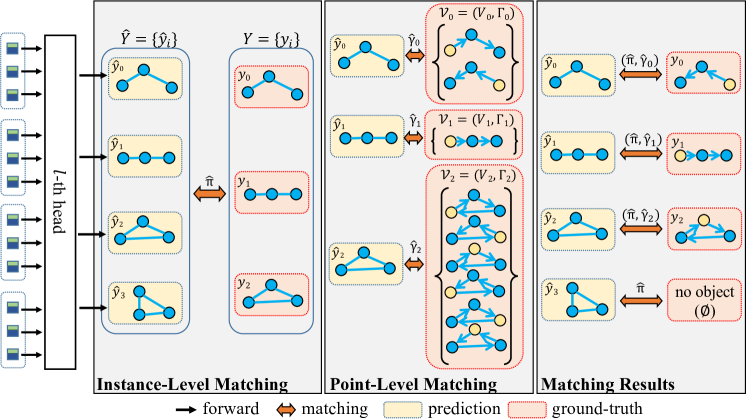
Figure 5: Hierarchical bipartite matching. MapTRv2 performs instance-level matching to find optimal instance-level assignment $\hat{\pi}$, and performs point-level matching to find optimal point-to-point assignment $\hat{\gamma}$ (Sec. 5.1). Based on the optimal instance-level and point-level assignments ($\hat{\pi}$ and $\{\hat{\gamma}_{i}\}$), one-to-one set prediction loss (Sec. 5.2) is defined for end-to-end learning.

4.2 Map Decoder

Map decoder consists of map queries and several decoder layers. Each decoder layer utilizes self-attention and cross-attention to update the map queries. We detail the specific design as following:

Hierarchical Query. We propose a hierarchical query embedding scheme to explicitly encode each map element. Specifically, we define a set of instance-level queries $\{q^{\rm{ins}}_{i}\}_{i=0}^{N-1}$ and a set of point-level queries $\{q^{\rm{pt}}_{j}\}_{j=0}^{N_{v}-1}$ shared by all instances. Each map element (with index $i$) corresponds to a set of hierarchical queries $\{q^{\rm{hie}}_{ij}\}_{j=0}^{N_{v}-1}$. The hierarchical query of $j$-th point of $i$-th map element is formulated as:

$$\begin{gathered}q^{\rm{hie}}_{ij}=q^{\rm{ins}}_{i}+q^{\rm{pt}}_{j}.\end{gathered}$$ (3)

Self-Attention Variants. MapTR [16] adopts vanilla self-attention to make hierarchical queries exchange information with each other (both inter-instance and intra-instance), whose computation complexity is $O((N\times N_{v})^{2})$ ($N$ and $N_{v}$ are respectively the numbers of instance queries and point queries). With the query number increasing, the computation cost and memory consumption dramatically increase.

In MapTRv2, to reduce the budget of computation and memory, we adopt decoupled self-attention, i.e., respectively performing attention along the inter-ins. dimension and intra-ins. dimension, as shown in Fig. 4. The decoupled self-attention greatly reduces the memory consumption and computation complexity (from $O((N\times N_{v})^{2})$ to $O(N^{2}+N_{v}^{2})$), and results in higher performance than vanilla self-attention.

Another variant is only performing inter-ins. self-attention. With only inter-ins. self-attention, MapTRv2 also achieves comparable performance (see Sec. 6.3).

Cross-Attention Variants. Cross-attention in the decoder is designed to make map queries interact with input features. We study on three kinds of cross-attention: BEV-based, PV-based and hybrid cross-attention.

For BEV-based cross-attention, we adopt Deformable Attention [57, 10] to make hierarchical queries interact with BEV features. For 2D map construction, each query $q^{\rm{hie}}_{ij}$ predicts the 2-dimension normalized BEV coordinate $(x_{ij},y_{ij})$ of the reference point $p_{ij}$. For 3D map construction, each query $q^{\rm{hie}}_{ij}$ predicts the 3-dimension normalized 3D coordinate $(x_{ij},y_{ij},z_{ij})$ of the reference point $p_{ij}$. We then sample BEV features around the reference points and update queries.

Map elements are usually with irregular shapes and require long-range context. Each map element corresponds to a set of reference points $\{p_{ij}\}_{j=0}^{N_{v}-1}$ with flexible and dynamic distribution. The reference points $\{p_{ij}\}_{j=0}^{N_{v}-1}$ can adapt to the arbitrary shape of map element and capture informative context for map element learning.

For PV-based cross-attention, we project the reference points $p_{ij}$ to the PV images and then sample features around the projected reference points. Dense BEV features are depreciated.

Hybrid cross-attention is a combination of the above two cross-attention manners. Ablation experiments about these cross-attention variants are presented in Sec. 6.3.

Prediction Head. The prediction head is simple, consisting of a classification branch and a point regression branch. The classification branch predicts instance class score. The point regression branch predicts the positions of the point sets $\hat{V}$. For each map element, it outputs a $2N_{v}$- or $3N_{v}$-dimension vector, which represents normalized 2d or 3d coordinates of the $N_{v}$ points.

5 Training

5.1 Hierarchical Bipartite Matching

MapTRv2 parallelly infers a fixed-size set of $N$ map elements in a single pass, following the end-to-end paradigm of query-based object detection and segmentation paradigm [13, 58, 65]. $N$ is set to be larger than the typical number of map elements in a scene. Let’s denote the set of $N$ predicted map elements by $\hat{Y}=\{\hat{y}_{i}\}_{i=0}^{N-1}$. The set of ground-truth (GT) map elements is padded with $\varnothing$ (no object) to form a set with size $N$, denoted by $Y=\{y_{i}\}_{i=0}^{N-1}$. $y_{i}=(c_{i},V_{i},\Gamma_{i})$, where $c_{i}$, $V_{i}$ and $\Gamma_{i}$ are respectively the target class label, point set and permutation group of GT map element $y_{i}$. $\hat{y}_{i}=(\hat{p}_{i},\hat{V}_{i})$, where $\hat{p}_{i}$ and $\hat{V}_{i}$ are respectively the predicted classification score and predicted point set. To achieve structured map element modeling and learning, MapTRv2 introduces hierarchical bipartite matching as shown in Fig. 5, i.e., performing instance-level matching and point-level matching in order.

Instance-Level Matching. First, we need to find an optimal instance-level label assignment $\hat{\pi}$ between predicted map elements $\{\hat{y}_{i}\}$ and GT map elements $\{y_{i}\}$. $\hat{\pi}$ is a permutation of $N$ elements ($\hat{\pi}\in\Pi_{N}$) with the lowest instance-level matching cost:

$$\begin{gathered}\hat{\pi}=\operatorname*{arg\,min}_{\pi\in\Pi_{N}}\sum_{i=0}^{N-1}\mathcal{L}_{\rm ins\_match}(\hat{y}_{\pi(i)},y_{i}).\end{gathered}$$ (4)

$\mathcal{L}_{\rm ins\_match}(\hat{y}_{\pi(i)},y_{i})$ is a pair-wise matching cost between prediction $\hat{y}_{\pi(i)}$ and GT $y_{i}$, which considers both the class label of map element and the position of point set:

$$\begin{gathered}\mathcal{L}_{\rm ins\_match}(\hat{y}_{{\pi}(i)},y_{i})=\mathcal{L}_{\rm{Focal}}(\hat{p}_{{\pi}(i)},c_{i})+\mathcal{L}_{\rm position}(\hat{V}_{\pi(i)},V_{i}).\end{gathered}$$ (5)

$\mathcal{L}_{\rm{Focal}}(\hat{p}_{{\pi}(i)},c_{i})$ is the class matching cost term, defined as the Focal Loss [78] between predicted classification score $\hat{p}_{{\pi}(i)}$ and target class label $c_{i}$. $\mathcal{L}_{\rm position}(\hat{V}_{\pi(i)},V_{i})$ is the position matching cost term, which reflects the position correlation between the predicted point set $\hat{V}_{\pi(i)}$ and the GT point set $V_{i}$. Hungarian algorithm is utilized to find the optimal instance-level assignment $\hat{\pi}$ following DETR [13].

Point-Level Matching. After instance-level matching, each predicted map element $\hat{y}_{\hat{\pi}(i)}$ is assigned with a GT map element $y_{i}$. Then for each predicted instance assigned with positive labels ($c_{i}\neq\varnothing$), we perform point-level matching to find an optimal point-to-point assignment $\hat{\gamma}\in\Gamma$ between predicted point set $\hat{V}_{\hat{\pi}(i)}$ and GT point set $V_{i}$. $\hat{\gamma}$ is selected among the predefined permutation group ${\Gamma}$ and with the lowest point-level matching cost:

$$\begin{gathered}\hat{\gamma}=\operatorname*{arg\,min}_{\gamma\in{\Gamma}}\sum_{j=0}^{N_{v}-1}D_{\rm{Manhattan}}(\hat{v}_{j},v_{\gamma(j)}).\end{gathered}$$ (6)

$D_{\rm{Manhattan}}(\hat{v}_{j},v_{\gamma(j)})$ is the Manhattan distance between the $j$-th point of the predicted point set $\hat{V}$ and the $\gamma(j)$-th point of the GT point set $V$.

5.2 One-to-One Set Prediction Loss

MapTRv2 is trained based on the optimal instance-level and point-level assignment ($\hat{\pi}$ and $\{\hat{\gamma_{i}}\}$). The basic loss function is composed of three parts, classification loss, point-to-point loss and edge direction loss:

$$\mathcal{L}_{\rm one2one}= \mathcal{L}_{\rm Hungarian}(\hat{Y},Y)$$ (7)

$$= \lambda_{c}\mathcal{L}_{\rm{cls}}+\lambda_{p}\mathcal{L}_{\rm{p2p}}+\lambda_{d}\mathcal{L}_{\rm{dir}},$$

where $\lambda_{c}$, $\lambda_{p}$ and $\lambda_{d}$ are the weights for balancing different loss terms.

Classification Loss. With the instance-level optimal matching result $\hat{\pi}$, each predicted map element is assigned with a class label . The classification loss is a Focal Loss term formulated as:

$$\begin{gathered}\mathcal{L}_{\rm{cls}}=\sum_{i=0}^{N-1}\mathcal{L}_{\rm{Focal}}(\hat{p}_{\hat{\pi}(i)},c_{i}).\end{gathered}$$ (8)

Point-to-Point Loss. Point-to-point loss supervises the position of each predicted point. For each GT instance with index $i$, according to the point-level optimal matching result $\hat{\gamma}_{i}$, each predicted point $\hat{v}_{\hat{\pi}(i),j}$ is assigned with a GT point $v_{i,\hat{\gamma}_{i}(j)}$. The point-to-point loss is defined as the Manhattan distance computed between each assigned point pair:

$$\begin{gathered}\mathcal{L}_{\rm{p2p}}=\sum_{i=0}^{N-1}\mathbbm{1}_{\{c_{i}\neq\varnothing\}}\sum_{j=0}^{N_{v}-1}D_{\rm{Manhattan}}(\hat{v}_{\hat{\pi}(i),j},v_{i,\hat{\gamma}_{i}(j)}).\end{gathered}$$ (9)

Edge Direction Loss. Point-to-point loss only supervises the node point of polyline and polygon, not considering the edge (the connecting line between adjacent points). For accurately representing map elements, the direction of the edge is important. Thus, we further design edge direction loss to supervise the geometrical shape in the higher edge level. Specifically, we consider the cosine similarity of the paired predicted edge $\bm{\hat{e}_{\hat{\pi}(i),j}}$ and GT edge $\bm{e_{i,\hat{\gamma}_{i}(j)}}$:

$$\begin{gathered}\mathcal{L}_{\rm{dir}}=-\sum_{i=0}^{N-1}\mathbbm{1}_{\{c_{i}\neq\varnothing\}}\sum_{j=0}^{N_{v}-1}{\rm cos\_similarity}(\bm{\hat{e}_{\hat{\pi}(i),j}},\bm{e_{i,\hat{\gamma}_{i}(j)}}),\\ \bm{\hat{e}_{\hat{\pi}(i),j}}=\hat{v}_{\hat{\pi}(i),j}-\hat{v}_{\hat{\pi}(i),(j+1)\rm{mod}N_{v}},\\ \bm{e_{i,\hat{\gamma}_{i}(j)}}=v_{i,\hat{\gamma}_{i}(j)}-v_{i,\hat{\gamma}_{i}(j+1)\rm{mod}N_{v}}.\end{gathered}$$ (10)

5.3 Auxiliary One-to-Many Set Prediction Loss

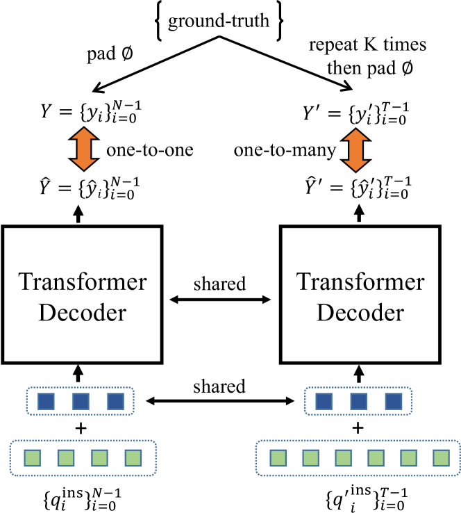
Figure 6: Auxiliary one-to-many matching branch. We introduce extra $T$ instance-level queries during training to provide auxiliary supervision. The point-level queries and Transformer decoder layers are shared by the two groups of instance queries. We perform one-to-one matching on the first group of instance queries, as demonstrated in Sec. 5, and perform one-to-many matching on the second group of instance queries by repeating the ground-truth map elements for $K$ times. The detailed matching procedure is the same as hierarchical bipartite matching.

To speed up the convergence, we add an auxiliary one-to-many matching branch during training, inspired by [79]. As shown in Fig. 6, the one-to-many matching branch shares the same point queries and Transformer decoder with one-to-one matching branch, but own an extra group of instance queries $\{q_{i}^{{}^{\prime}\rm ins}\}_{i=0}^{T-1}$ ($T$ is the number). This branch predict map elements $\hat{Y}^{{}^{\prime}}=\{\hat{y}^{{}^{\prime}}_{i}\}_{i=0}^{T-1}$.

We repeat the ground-truth map elements for $K$ times and pad them with $\varnothing$ to form a set with size $T$, denoted by $Y^{{}^{\prime}}=\{y^{{}^{\prime}}_{i}\}_{i=0}^{T-1}$. Then we perform the same hierarchical bipartite matching between $\widetilde{Y}$ and $\overline{Y}$, and compute the auxiliary one-to-many set prediction loss:

$$\mathcal{L}_{\rm one2many}= \mathcal{L}_{\rm Hungarian}(\hat{Y}^{{}^{\prime}},Y^{{}^{\prime}})$$ (11)

In the one-to-many matching branch, one GT element is assigned to $K$ predicted elements. With the ratio of positive samples increasing, the map decoder converges faster.

5.4 Auxiliary Dense Prediction Loss

To further leverage semantic and geometric information, we introduce three auxiliary dense prediction losses:

$$\mathcal{L}_{\rm dense}= \alpha_{d}\mathcal{L}_{\rm{depth}}+\alpha_{b}\mathcal{L}_{\rm{BEVSeg}}+\alpha_{p}\mathcal{L}_{\rm{PVSeg}}.$$ (12)

Depth Prediction Loss. Following BEVDepth [74], we utilize the LiDAR point clouds to render the GT depth maps $\{D_{1},\ldots,D_{M}\}$ of each perspective view. And we add a simple depth prediction head $\phi_{\rm depth}$ on the PV feature map $\mathcal{F}=\{F_{1},\ldots,F_{M}\}$. The depth prediction loss is defined as the cross-entropy loss between the predicted depth map and the rendered GT depth map:

$$\mathcal{L}_{\rm depth}=\sum_{m=1}^{M}\mathcal{L}_{\rm CE}(\phi_{\rm depth}(F_{m}),D_{m}).$$ (13)

BEV Segmentation Loss. We add an auxiliary BEV segmentation head $\phi_{\rm BEVSeg}$ base on the BEV feature map $F_{BEV}$. We rasterize the map GT on the BEV canvas to get BEV foreground mask $M_{BEV}$. The BEV segmentation loss is defined as the cross entropy loss between the predicted BEV segmentation map and the binary GT map mask:

$$\mathcal{L}_{\rm BEVSeg}=\mathcal{L}_{\rm CE}(\phi_{\rm BEVSeg}(F_{BEV}),M_{BEV}).$$ (14)

PV Segmentation Loss. To fully exploit the dense supervision, we render map GT on the perspective views with intrinsics and extrinsics of cameras and get perspective foreground masks $\{M^{1}_{PV},\ldots,M^{1}_{PV}\}$. And we add a auxiliary PV segmentation head $\phi_{\rm PVSeg}$ on the PV feature map $\mathcal{F}=\{F_{1},\ldots,F_{M}\}$. The PV segmentation loss $\mathcal{L}_{\rm PVSeg}$ is defined as:

$$\mathcal{L}_{\rm PVSeg}=\sum_{m=1}^{M}\mathcal{L}_{\rm CE}(\phi_{\rm PVSeg}(F_{m}),M^{m}_{PV}).$$ (15)

5.5 Overall Loss

The overall loss is defined as the weighted sum of the above losses:

$$\mathcal{L}=\beta_{o}\mathcal{L}_{\rm{one2one}}+\beta_{m}\mathcal{L}_{\rm{one2many}}+\beta_{d}\mathcal{L}_{\rm{dense}}.$$ (16)

Method	Modality	Backbone	Epoch	AP				FPS
				ped.	div.	bou.	mean
HDMapNet	C	Effi-B0	30	14.4	21.7	33.0	23.0	0.9
	L	PP	30	10.4	24.1	37.9	24.1	1.1
	C & L	Effi-B0 & PP	30	16.3	29.6	46.7	31.0	0.5
VectorMapNet	C	R50	110+ft	42.5	51.4	44.1	46.0	2.2
	L	PP	110	25.7	37.6	38.6	34.0	-
	C & L	R50 & PP	110+ft	48.2	60.1	53.0	53.7	-
MapTR	C	R18	110	39.6	49.9	48.2	45.9	35.0
	C	R50	110	56.2	59.8	60.1	58.7	15.1
	C	R50	24	46.3	51.5	53.1	50.3	15.1
	L	Sec	24	48.5	53.7	64.7	55.6	8.0
	C & L	R50 & Sec	24	55.9	62.3	69.3	62.5	6.0
MapTRv2	C	R18	110	46.9	55.1	54.9	52.3	33.7
	C	R50	110	68.1	68.3	69.7	68.7	14.1
	C	V2-99	110	71.4	73.7	75.0	73.4	9.9
	C	R50	24	59.8	62.4	62.4	61.5	14.1
	C	V2-99	24	63.6	67.1	69.2	66.6	9.9
	L	Sec	24	56.6	58.1	69.8	61.5	7.6
	C & L	R50 & Sec	24	65.6	66.5	74.8	69.0	5.8

TABLE I: Comparisons with state-of-the-art methods [12, 11] on nuScenes val set. “C” and “L” respectively denotes camera and LiDAR. “ft” means fine-tuning, a training tirck illustrated in VectorMapNet [12]. “Effi-B0”, “R18”, “R50”, “V2-99”, “PP” and “Sec” respectively correspond to EfficientNet-B0 [80], ResNet18 [81], ResNet50 [81], VoVNetV2-99 [82], PointPillars [83] and LiDAR backbone used in SECOND [84]. Effi-B0, Effi-B4, R50 and R18 are initialized with ImageNet [85] pre-trained weights. V2-99 is initialized from DD3D [86] checkpoint. Other LiDAR backbones are trained from scratch. The APs of other methods are taken from the papers [12]. FPSs are measured on the same machine with RTX 3090. “-” means that the corresponding results are not available.

Method	Map dim.	Backbone	Epoch	AP				FPS
				ped.	div.	bou.	mean
HDMapNet	2	Effi-B0	-	13.1	5.7	37.6	18.8	-
VectorMapNet	2	R50	-	38.3	36.1	39.2	37.9	-
	3	R50	-	36.5	35.0	36.2	35.8	-
MapTRv2	2	R50	6	62.9	72.1	67.1	67.4	12.1
	3	R50	6	60.7	68.9	64.5	64.7	12.0

TABLE II: Comparisons with state-of-the-art methods [12, 11] on Argoverse2 val set. Argoverse2 provides 3D vectorized map, which has extra height information compared to nuScenes dataset. $\rm{dim}=2$ denotes that the height information of vectorized map is dropped. $\rm{dim}=3$ denotes directly predicting 3D vectorized map. The results of VectorMapNet and HDMapNet are taken from VectorMapNet paper [12]. FPSs are measured on the same machine with RTX 3090. “-” means that the corresponding results are not available.

6 Experiments

In this section, we first introduce our experimental setup and implementation details in Sec. 6.1. Then we present the main results of our frameworks and compare with state-of-the-art methods in Sec. 6.2. And in Sec. 6.3, we conduct extensive ablation experiments and analyses to investigate the individual components of our framework. In Sec. 6.2 and Sec. 6.4, we show that our framework is easily to be extended to 3D map construction and centerline learning.

6.1 Experimental Setup

Datasets. We mainly evaluate our method on the popular nuScenes [14] dataset following the standard setting of previous methods [11, 12, 16]. The nuScenes dataset contains 2D city-level global vectorized maps and 1000 scenes of roughly 20s duration each. Key samples are annotated at $2$Hz. Each sample has RGB images from $6$ cameras and covers $360^{\circ}$ horizontal FOV of the ego-vehicle.

We further provide experiments on Argoverse2 [15] dataset, which contains 1000 logs. Each log provides 15s of 20Hz RGB images from 7 cameras and a log-level 3D vectorized map.

Metric. We follow the standard metric used in previous works [11, 12, 16]. The perception ranges are $[-15.0m,15.0m]$ for the $X$-axis and $[-30.0m,30.0m]$ for the $Y$-axis. And we adopt average precision (AP) to evaluate the map construction quality. Chamfer distance $D_{Chamfer}$ is used to determine whether the prediction and GT are matched or not. We calculate the $\rm{AP}_{\tau}$ under several $D_{Chamfer}$ thresholds ($\tau\in T,T=\{0.5,1.0,1.5\}$), and then average across all thresholds as the final AP metric:

$$\rm{AP}=\frac{1}{|T|}\sum_{\tau\in T}\rm{AP}_{\tau}.$$ (17)

Following the previous methods  [11, 12, 16], three kinds of map elements are chosen for fair evaluation [12, 16, 11] – pedestrian crossing, lane divider, and road boundary. Besides, we also extend MapTRv2 to modeling and learning centerline (see Sec. 6.4) and provide additional evaluation.

Training Details. ResNet50 [81] is used as the image backbone network unless otherwise specified. The optimizer is AdamW with weight decay 0.01. The batch size is 32 (containing 6 view images) and all models are trained with 8 NVIDIA GeForce RTX 3090 GPUs. Default training schedule is 24 epochs and the initial learning rate is set to $6\times 10^{-4}$ with cosine decay. We extract ground-truth map elements in the perception range of ego-vehicle following [16, 12, 11]. The resolution of source nuScenes images is $1600\times 900$. For the real-time version, we resize the source image with 0.2 ratio and the other models are trained with 0.5-ratio-resized images. For Argoverse2 dataset, the 7 camera images have different resolutions ($1550\times 2048$ for front view and $2048\times 1550$ for others). We first pad the 7 camera images into the same shape ($2048\times 2048$), then resize the images with 0.3 ratio. Color jitter is used by default in both nuScenes dataset and Argoverse2 dataset. The default number of instance queries, point queries and decoder layers is 50, 20 and 6, respectively. For PV-to-BEV transformation, we set the size of each BEV grid to 0.3m and utilize efficient BEVPoolv2 [77] operation. Following [16], $\lambda_{c}=2$, $\lambda_{p}=5$, $\lambda_{d}=0.005$. For dense prediction loss, we set $\alpha_{d}$, $\alpha_{p}$, $\alpha_{b}$ to 3, 2 and 1 respectively. For the overall loss, $\beta_{o}=1$, $\beta_{m}=1$, $\beta_{d}=1$. We also provide long training schedule (110 epochs) on nuScenes dataset without changing other hyper-parameters for fair comparison with previous methods [12].

Inference Details. The inference stage is quite simple. Given surrounding images, we can directly predict 50 map elements associated with their scores. The scores indicate the confidence of predicted map element. The top-scoring predictions can be directly utilized without other post-processing. The inference time is measured on a single NVIDIA GeForce RTX 3090 GPU with batch size 1.

6.2 Main results

Comparison with State-of-the-Art Methods. We train MapTR/MapTRv2 under 24-epoch schedule and 110-epoch schedule on nuScenes dataset. As shown in Table I, MapTR/MapTRv2 outperforms all the state-of-the-art methods by a large margin in terms of convergence, accuracy and speed. Surprisingly, MapTRv2 based on ResNet-50 achieves 68.7 mAP, which 10 mAP higher than corresponding MapTR counterpart with similar speed and 6 mAP higher than the previous best-performing multi-modality result while being 2x faster. MapTRv2-VoVNet99 with only camera input achieves 73.4 mAP, which is 19.7 mAP higher than multi-modality VectorMapNet while being 4x faster and 10.9 mAP higher than multi-modality MapTR as well as 3.9 FPS faster. As shown in Fig. 1, MapTR/MapTRv2 achieves the best trade-off between accuracy and speed. MapTRv2-ResNet18 achieves 50+ mAP at the real-time speed.

Meanwhile, we also evaluate our framework on the Argoverse2 dataset. Argoverse2 provides 3D vectorized map, which has extra height information compared to nuScenes dataset. As shown in Table II, In terms of 2D vectorized map construction, MapTRv2 achieves 67.4 mAP, which is 29.5 mAP higher than VectorMapNet and 48.6 mAP higher than HDMapNet. In terms of 3D vectorized map construction, MapTRv2 achieves 64.7 mAP, which is 29.9 mAP higher than VectorMapNet. The experiments on Argoverse2 dataset demonstrates the superior generalization ability of MapTRv2 in terms of 3D vectorized map construction.

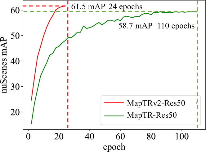
Figure 7: Convergence curves of MapTRv2 and MapTR with ResNet-50 backbone on nuScenes dataset. MapTRv2 significantly outperforms MapTR with 4x shorter training schedule and 2.8 higher mAP.

Roadmap of MapTRv2. In Table III, we show how we build MapTRv2 upon MapTR. We first replace the default PV-to-BEV transformation method GKT in MapTR with LSS. Then we gradually add the auxiliary dense supervision, memory-efficient decoupled self-attention and auxiliary one-to-many matching. With all these components, MapTRv2-ResNet50 achieves 61.5 mAP, which is 11.1 mAP higher than MapTR-ResNet50 with similar speed. As shown in Fig. 7, MapTRv2 achieves superior convergence than MapTR (24 epochs, 61.5 mAP vs. 110 epochs, 58.7mAP). We also provide a BEV-free variant of MapTRv2 by replacing the BEV-based cross-attention with PV-based cross-attention and removing PV-to-BEV transformation module. Though the performance of BEV-free MapTRv2 drops, this variant gets rid of costly dense BEV representation and is more lightweight.

Method	mAP	AP
		ped.	div.	bou.
MapTR baseline	50.3	46.3	51.5	53.1
+2D-to-BEV with LSS	50.1 (-0.2)	44.9	51.9	53.5
+auxiliary depth sup.	55.2 (+4.9)	49.6	56.6	59.4
+auxiliary BEV sup.	56.5 (+6.2)	52.1	57.6	59.9
+auxiliary PV sup.	57.1 (+6.8)	53.2	58.1	60.0
+decoupled self-attn.	57.6 (+7.3)	53.9	58.3	60.5
+one-to-many matching	61.5 (+11.1)	59.8	62.4	62.4
+BEV free (optional)	49.5 (-12.0)	42.5	52.0	53.4

TABLE III: Roadmap of MapTRv2 on nuScenes val set with only 24-epoch training schedule.

Shape Modeling	AP
	ped.	div.	bou.	mean
Fixed-order $V^{F}$ w/ ambiguity	52.7	59.1	60.3	57.4
Permutation-equivalent $(V,\Gamma)$ w/o ambiguity	gray!3059.8	gray!3062.4	gray!3062.4	gray!3061.5

TABLE IV: Ablation on the permutation-equivalent shape modeling. Our proposed permutation-equivalent shape modeling outperforms the fixed-order shape modeling by 4.1 mAP and 7.1 AP in pedestrian-crossing especially.

6.3 Ablation Study

In this section, we investigate the individual components of our MapTRv2 framework with extensive ablation experiments. We conduct all experiments on the popular nuScenes dataset unless otherwise specified. For efficiently conducting the ablation experiments, we use MapTRv2-ResNet50 with 24-epoch training schedule as the baseline model unless otherwise specified.

Permutation Equivalent Modeling. In Table IV, we provide ablation experiments to validate the effectiveness of the proposed permutation-equivalent modeling. Compared with vanilla modeling method which imposes a unique permutation to the point set, permutation-equivalent modeling solves the ambiguity of map element and brings an improvement of 4.1 mAP. For pedestrian crossing, the improvement even reaches 7.1 AP, proving the superiority in modeling polygon elements.

Self-Attention Variants. In this ablation study, we remove the hybrid matching to fully reveal the efficiency of self-attention variants. As shown in Table V, the instance self-attention largely reduces the training memory (2265M memory reduction) while at cost of negligible accuracy drop (0.3 mAP drop). To recover the interaction in each instance, decoupled self-attention adds one more self-attention on point-dim. It is much more memory-efficient (1985M memory reduction) and achieves better accuracy (0.5 mAP higher) and similar speed compared with vanilla self-attention. To further reveal superiority of the decoupled self-attention, in Table VI, we compare vanilla self-attention with decoupled self-attention in terms of memory consumption and the number of instance queries. with the number of instance queries increasing, mAP and memory cost consistently increases. Under the same memory limitation (24 GB of RTX 3090), decoupled self-attention requires much less memory and results in higher performance upper bound.

Self-Attn	AP				GPU mem.	FPS
	ped.	div.	bou.	mean
Vanilla	53.2	58.1	60.0	57.1	10443 M	14.7
Only inter-ins.	53.1	57.2	60.2	56.8	8178 M	14.9
Decoupled	53.9	58.3	60.5	57.6	8458 M	14.1

TABLE V: Ablation on the self-attention variants. The inter self-attention demonstrates significant memory reduction while maintaining comparable accuracy. We choose the decoupled self-attention as the default configuration.

N	50	75	100	125	150
mAP+	57.1	58.4	59.5	-	-
GPU memory+ (M)	10443	13720	18326	OOM	OOM
mAP∗	57.6	60.1	60.3	60.4	61.2
GPU memory∗ (M)	8458	9049	9670	10378	11157

TABLE VI: Comparisons between vanilla self-attention and decoupled self-attention in terms of memory consumption and number of instance queries. “+” denotes the results of vanilla self-attention, “*” denotes the results of decoupled self-attention. “OOM” denotes out of memory. “-” denotes the results are not available. When the number of instance queries reaches 125, the training memory of vanilla self-attention exceeds the RTX 3090 GPU memory. The decoupled self-attention significantly reduces the training memory and consistently outperforms the vanilla self-attention.

Cross-Attention Variants. In Table VII, we ablate on cross-attention on nuScenes dataset and Argoverse2 dataset. Height information of map is not available on nuScenes dataset, thus the projected reference points on PV features are not accurate enough. When we simply replace the BEV-based deformable cross-attention with the PV-based one, the accuracy drops by 12.0 mAP. When we stack the BEV-based and PV-based cross-attention, the performance is still inferior to that of BEV-based one. But on Argoverse2 dataset, height information of map is available and the projected reference points can be supervised to be accurate. So the performance gap between BEV-based and PV-based cross-attention is much smaller compared to that on nuScenes. And the hybrid cross-attention improves the BEV-based accuracy by 0.9 mAP, demonstrating the complementarity of PV features and BEV features.

Dense Prediction Loss. In Table VIII, we ablate on the effectiveness of dense supervision. The results show that depth supervision, PV segmentation and BEV segmentation provide complementary supervision. By adding them together, the final performance is improved by 4.9 mAP.

Dataset	Cross-Attn	AP				FPS
		ped.	div.	bou.	mean
nus. 2D	BEV	gray!3059.8	gray!3062.4	gray!3062.4	gray!3061.5	gray!3014.1
	PV	42.5	52.0	53.4	49.5	14.4
	BEV + PV	58.9	60.6	62.0	60.5	11.5
av2. 3D	BEV	gray!3060.7	gray!3068.9	gray!3064.5	gray!3064.7	gray!3012.0
	PV	53.1	63.4	60.8	59.1	12.7
	BEV + PV	61.4	69.9	65.6	65.6	10.0

TABLE VII: Ablation on the cross-attention variants on nuScenes and Argoverse2. “nus. 2D” denotes that nuScenes dataset only provides 2D vectorized maps, lacking in height information. “av2. 3D” denotes that Argoverse2 provides 3D vectorized maps. “BEV” denotes BEV-based cross-attention. “PV” denotes PV-based cross-attention. “BEV + PV” denotes the hybrid cross-attention. We choose the BEV-based cross-attention as the default configuration.

Depth	Seg${}^{\text{PV}}$	Seg${}^{\text{BEV}}$	AP				FPS
			ped.	div.	bou.	mean
			53.4	58.8	57.5	56.6	14.1
✓			57.3	60.5	61.7	59.8	14.1
✓	✓		58.8	61.3	61.4	60.5	14.1
✓		✓	60.1	61.3	61.6	61.0	14.1
	✓	✓	57.5	60.5	59.7	59.2	14.1
gray!30✓	gray!30✓	gray!30✓	gray!3059.8	gray!3062.4	gray!3062.4	gray!30 61.5	gray!3014.1

TABLE VIII: Ablation on the auxiliary dense prediction losses. “Depth” denotes depth prediction loss. “Seg^PV” denotes PV segmentation loss. “Seg^BEV” denotes BEV segmentation loss. Each of them provides complementary supervision.

One-to-Many Loss. We ablate on the hyper-parameter $K$ in Table IX. With $K$ increasing, the training memory cost correspondingly increases. Due to the limited GPU memory, we only increase $K$ up to 6, which brings an improvement of 3.9 mAP. And in Table X, we fix $K=6$ and ablate on $T$. The results show consistent improvement from $T=100$ to $T=300$. We further ablate on the hyper-parameter $\beta_{m}$ of auxiliary one-to-many loss in Table XI. Finally, we choose $T=300$, $K=6$, $\lambda=1$ as the default setting of MapTRv2.

$K$	0	1	2	3	4	5	gray!306
mAP	57.6	58.7	61.0	60.9	60.9	60.9	gray!3061.5
GPU mem.(M)	8458	9670	11157	12875	14814	17004	gray!3019426
FPS	14.1	14.1	14.1	14.1	14.1	14.1	gray!3014.1

TABLE IX: Ablation on $K$ in hybrid matching. We set $T=50\times K$.

$T$	100	150	200	250	gray!30300
mAP	58.0	59.6	60.3	61.4	gray!3061.5
GPU mem.(M)	11157	12875	14814	17004	gray!3019426
FPS	14.1	14.1	14.1	14.1	gray!3014.1

TABLE X: Ablation on $T$ in hybrid matching. We set $K=6$.

$\beta_{m}$	0.1	0.2	0.5	gray!301.0	2.0	5.0
mAP	58.5	59.3	60.6	gray!3061.5	59.9	60.4

TABLE XI: Ablation on $\beta_{m}$. We set $K=6$ and $T=300$. We choose $\beta_{m}=1.0$ as the default configuration.

Point	AP				Param.	FPS
	ped.	div.	bou.	mean
10	55.3	64.1	60.5	60.0	39.0	14.1
gray!3020	gray!3059.8	gray!3062.4	gray!3062.4	gray!3061.5	gray!3039.0	gray!3014.1
30	56.7	58.7	61.8	59.0	39.0	14.0
40	55.1	54.8	61.0	56.9	39.0	14.2

TABLE XII: Ablation on the number of point queries. We choose 20 point queries as the default configuration.

Input Modality. As shown in Table I, our framework is compatible with other vehicle-mounted sensors like LiDAR. Multi-modality MapTRv2 achieves superior performance (7.5 mAP higher) than single-modality MapTRv2 under 24-epoch training schedule, demonstrating the complementarity of different sensor inputs. And we reduce the gap between camera-only and LiDAR-only from 5.3 mAP in MapTR to 0.0 mAP in MapTRv2.

The Number of Points. In Table XII, we ablate on the point number of each element. The results show that 20 points are enough to achieve the best performance. Further increasing the point number increases the optimization difficulty and leads to performance drop. We choose 20 points as the default configuration.

The Number of Transformer Decoder Layers. Map decoder layers iteratively update the predicted map. Table XIII shows the ablation about the number of decoder layers. Without the iterative architecture, the result is 39.5 mAP. Increasing to 2 layers brings a gain of 13.1 mAP. The performance is saturated at 6 layers. We choose 6 layers as the default configuration.

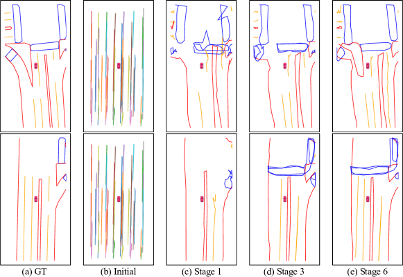
Figure 8: Iterative refinement. Column (a) is the ground-truth vectorized map. Column (b) is the map predicted by initial queries, in which different colors indicate different instances. Column (c) and (d) are the intermediate results after 1 and 3 Transformer decode layers, respectively. Column (e) is the final results. For column (c), (d) and (e), we only visualize those predicted map elements whose classification scores are above 0.3. The initial queries serve as priors of map. The cascade Transformer decoder layers iteratively refine positions and remove duplicate ones.

Iterative Refinement. In Fig. 8, we show the procedure of iterative refinement of a converged MapTRv2 baseline model by visualizing the predicted map elements at different decoder layers. The initial queries seem like evenly distributed polylines with different lengths (Fig. 8 (b)), which serve as the priors of map. The cascaded decoder layers gradually refine the predictions and remove duplicate ones, as shown in Fig. 8 (c), (d) and (e).

Detailed Runtime. In Table XIV, we provide the detailed runtime of each component in MapTRv2-ResNet50 with only camera input. The results show that the main inference cost lies in the backbone network (59.8%) while the other modules are quite efficient.

Robustness to the Camera Deviation. In real applications, the camera intrinsics are usually accurate and change little, but the camera extrinsics may be inaccurate due to the shift of camera position, calibration error, etc. To validate the robustness, we traverse the validation sets and randomly generate noise for each sample. We respectively add translation and rotation deviation of different degrees. Note that we add noise to all cameras and all coordinates. And the noise is subject to normal distribution. There exists extremely large deviation in some samples, which affect the performance a lot. As illustrated in Table XV and Table XVI, when the standard deviation of $\Delta_{x},\Delta_{y},\Delta_{z}$ is $0.1m$ or the standard deviation of $\theta_{x},\theta_{y},\theta_{z}$ is $0.01rad$, MapTRv2 still keeps comparable performance.

Layer	AP				Param.	FPS
	ped.	div.	bou.	mean
1	32.0	42.8	43.7	39.5	32.9	17.9
2	46.0	54.7	57.0	52.6	34.1	16.9
3	53.2	57.6	59.7	56.8	35.3	16.0
gray!306	gray!3059.8	gray!30 62.4	gray!3062.4	gray!3061.5	gray!3039.0	gray!3014.1
8	60.2	62.3	61.4	61.3	41.4	13.1

TABLE XIII: Ablation on the number of Transformer decoder layers. Gradually increasing the number of decoder layers results in lower inference speed and higher accuracy. The accuracy is saturated at 6 Transformer decoder layers. We choose 6 Transformer decoder layers as the default configuration.

6.4 Extention: Centerline

Centerline can be seen as an special type of map elements, which provide directional information, indicate the traffic flow and play an important role in downstream planners as demonstrated in [87]. Following the path-wise modeling proposed in LaneGAP [32], we include centerline learning in MapTRv2. As shown in Table XVII, with centerline included, MapTRv2 achieves 54.0 mAP on nuScenes dataset, and 62.6 mAP (2D map) / 61.4 mAP (3D map) on Argoverse2 dataset. Extending MapTRv2 to centerline paves the way for end-to-end planning.

Component	Runtime (ms)	Proportion
Backbone	42.4	59.8%
PV2BEV module	11.6	16.4%
Map decoder	16.9	23.8%
Total	70.9	100%

TABLE XIV: Detailed runtime of each component in MapTRv2-ResNet50 on one RTX 3090 GPU.

$\sigma_{1}(m)$	0	0.05	0.1	0.5	1.0
mAP	61.5	60.8	58.0	50.6	32.3

TABLE XV: Robustness to the translation deviation of camera. $\sigma_{1}$ is the standard deviation of $\Delta_{x},\Delta_{y},\Delta_{z}$.

$\sigma_{2}(rad)$	0	0.005	0.01	0.02	0.05
mAP	61.5	61.2	59.8	35.6	18.8

TABLE XVI: Robustness to the rotation deviation of camera. $\sigma_{2}$ is the standard deviation of $\theta_{x},\theta_{y},\theta_{z}$.

Dataset	Dim	Epoch	AP
			ped.	div.	bou.	cen.	mean
nuScenes	2	24	50.1	53.9	58.8	53.1	54.0
Argoverse2	2	6	55.2	67.2	64.8	63.2	62.6
Argoverse2	3	6	53.5	66.9	63.6	61.5	61.4

TABLE XVII: Performance with centerline learning. The mAP of centerline is as high as those of other elements. The results show that MapTRv2 is highly extensible and compatible to different map elements.

6.5 Qualitative Results

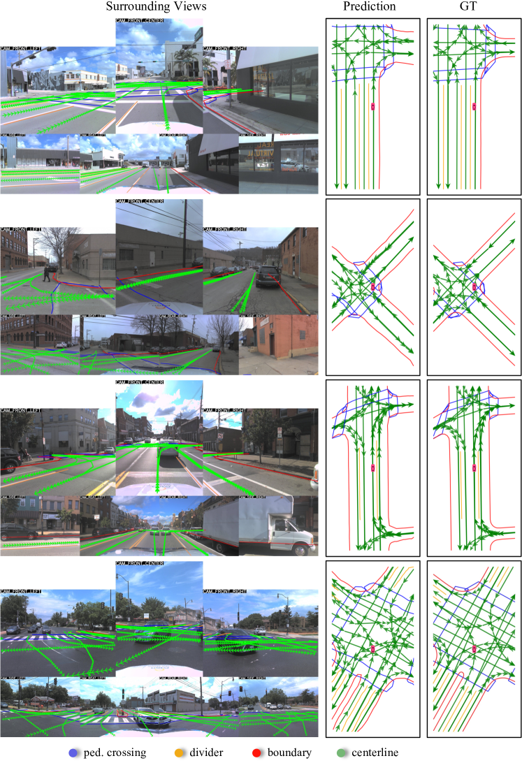
Figure 9: Qualitative results on Argoverse2 val set. Since we predict 3D vectorized HD map, the predictions can be accurately rendered on the surrounding view images.

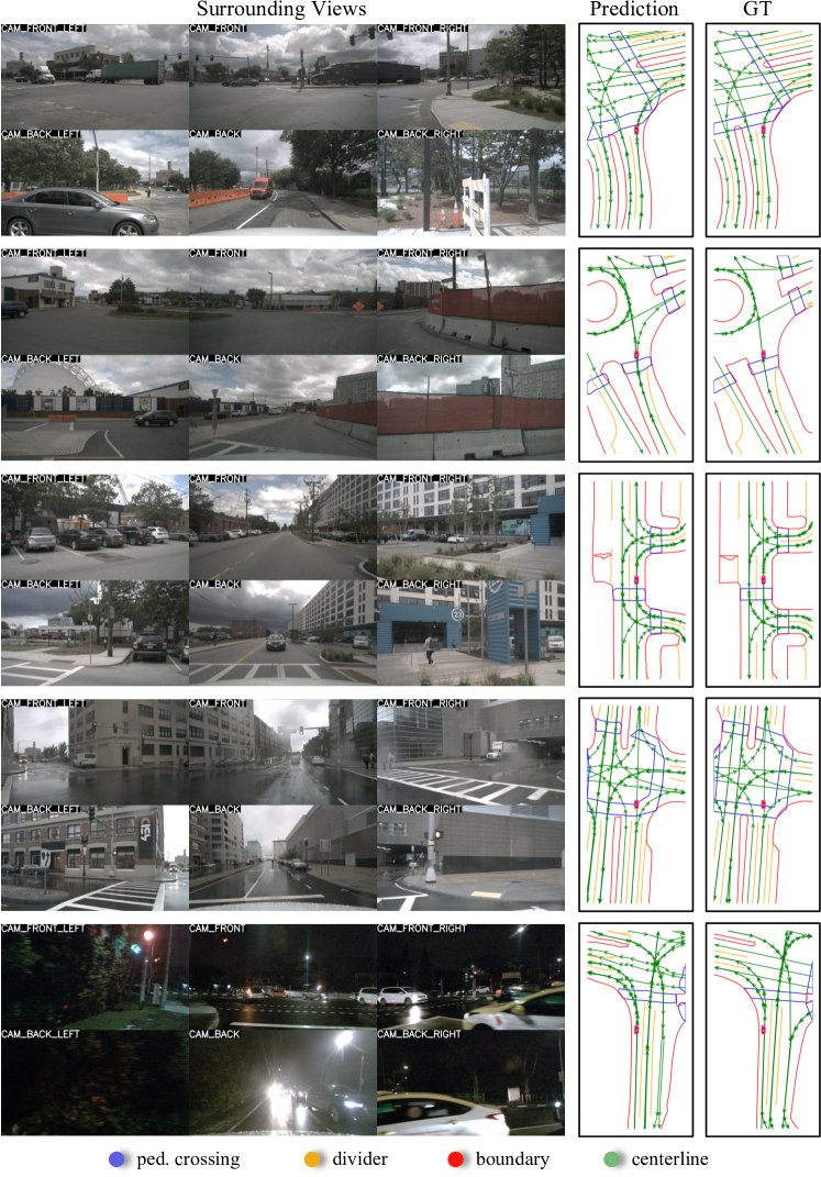
Figure 10: Qualitative results on nuScenes val set.

We show the predicted vectorized HD map results of Argoverse2 and nuScenes datasets respectively in Fig. 9 and Fig. 10. MapTRv2 maintains stable and impressive results in complex and various driving scenes. More qualitative results are available at the project website https://github.com/hustvl/MapTR.

7 Conclusion

MapTRv2 is a structured end-to-end framework for efficient online vectorized HD map construction, which adopts a simple encoder-decoder Transformer architecture and hierarchical bipartite matching to perform map element learning based on the proposed permutation-equivalent modeling. Extensive experiments show that the proposed method can precisely perceive map elements of arbitrary shape in both nuScenes and Argoverse2 datasets. We hope MapTRv2 can serve as a basic module of self-driving system and boost the development of downstream tasks (e.g., motion prediction and planning).

References

- [1] J. Zhang and S. Singh, “LOAM: lidar odometry and mapping in real-time,” in Robotics: Science and Systems X, University of California, 2014.
- [2] T. Shan and B. Englot, “Lego-loam: Lightweight and ground-optimized lidar odometry and mapping on variable terrain,” in IROS, 2018.
- [3] T. Shan, B. J. Englot, D. Meyers, W. Wang, C. Ratti, and D. Rus, “LIO-SAM: tightly-coupled lidar inertial odometry via smoothing and mapping,” in IROS, 2020.
- [4] L. Chen, C. Sima, Y. Li, Z. Zheng, J. Xu, X. Geng, H. Li, C. He, J. Shi, Y. Qiao, and J. Yan, “Persformer: 3d lane detection via perspective transformer and the openlane benchmark,” in ECCV, 2022.
- [5] R. Liu, Z. Yuan, T. Liu, and Z. Xiong, “End-to-end lane shape prediction with transformers,” in WACV, 2021.
- [6] Y. B. Can, A. Liniger, D. P. Paudel, and L. Van Gool, “Structured bird’s-eye-view traffic scene understanding from onboard images,” in ICCV, 2021.
- [7] S. Chen, T. Cheng, X. Wang, W. Meng, Q. Zhang, and W. Liu, “Efficient and robust 2d-to-bev representation learning via geometry-guided kernel transformer,” arXiv preprint arXiv:2206.04584, 2022.
- [8] B. Zhou and P. Krähenbühl, “Cross-view transformers for real-time map-view semantic segmentation,” in CVPR, 2022.
- [9] A. Hu, Z. Murez, N. Mohan, S. Dudas, J. Hawke, V. Badrinarayanan, R. Cipolla, and A. Kendall, “FIERY: Future instance segmentation in bird’s-eye view from surround monocular cameras,” in ICCV, 2021.
- [10] Z. Li, W. Wang, H. Li, E. Xie, C. Sima, T. Lu, Y. Qiao, and J. Dai, “Bevformer: Learning bird’s-eye-view representation from multi-camera images via spatiotemporal transformers,” in ECCV, 2022.
- [11] Q. Li, Y. Wang, Y. Wang, and H. Zhao, “Hdmapnet: An online hd map construction and evaluation framework,” in ICRA, 2022.
- [12] Y. Liu, Y. Wang, Y. Wang, and H. Zhao, “Vectormapnet: End-to-end vectorized hd map learning,” arXiv preprint arXiv:2206.08920, 2022.
- [13] N. Carion, F. Massa, G. Synnaeve, N. Usunier, A. Kirillov, and S. Zagoruyko, “End-to-end object detection with transformers,” in ECCV, 2020.
- [14] H. Caesar, V. Bankiti, A. H. Lang, S. Vora, V. E. Liong, Q. Xu, A. Krishnan, Y. Pan, G. Baldan, and O. Beijbom, “nuscenes: A multimodal dataset for autonomous driving,” in CVPR, 2020.
- [15] B. Wilson, W. Qi, T. Agarwal, J. Lambert, J. Singh, S. Khandelwal, B. Pan, R. Kumar, A. Hartnett, J. K. Pontes et al., “Argoverse 2: Next generation datasets for self-driving perception and forecasting,” arXiv preprint arXiv:2301.00493, 2023.
- [16] B. Liao, S. Chen, X. Wang, T. Cheng, Q. Zhang, W. Liu, and C. Huang, “MapTR: Structured modeling and learning for online vectorized HD map construction,” in The Eleventh International Conference on Learning Representations, 2023. [Online]. Available: https://openreview.net/forum?id=k7p_YAO7yE
- [17] Y. Ma, T. Wang, X. Bai, H. Yang, Y. Hou, Y. Wang, Y. Qiao, R. Yang, D. Manocha, and X. Zhu, “Vision-centric bev perception: A survey,” arXiv preprint arXiv:2208.02797, 2022.
- [18] H. Li, C. Sima, J. Dai, W. Wang, L. Lu, H. Wang, E. Xie, Z. Li, H. Deng, H. Tian et al., “Delving into the devils of bird’s-eye-view perception: A review, evaluation and recipe,” arXiv preprint arXiv:2209.05324, 2022.
- [19] J. Philion and S. Fidler, “Lift, splat, shoot: Encoding images from arbitrary camera rigs by implicitly unprojecting to 3d,” in ECCV, 2020.
- [20] Z. Liu, S. Chen, X. Guo, X. Wang, T. Cheng, H. Zhu, Q. Zhang, W. Liu, and Y. Zhang, “Vision-based uneven bev representation learning with polar rasterization and surface estimation,” arXiv preprint arXiv:2207.01878, 2022.
- [21] Z. Liu, H. Tang, A. Amini, X. Yang, H. Mao, D. Rus, and S. Han, “Bevfusion: Multi-task multi-sensor fusion with unified bird’s-eye view representation,” arXiv preprint arXiv:2205.13542, 2022.
- [22] C. Pan, Y. He, J. Peng, Q. Zhang, W. Sui, and Z. Zhang, “Baeformer: Bi-directional and early interaction transformers for bird’s eye view semantic segmentation,” in Proceedings of the IEEE/CVF Conference on Computer Vision and Pattern Recognition, 2023, pp. 9590–9599.
- [23] Z. Qin, J. Chen, C. Chen, X. Chen, and X. Li, “Uniformer: Unified multi-view fusion transformer for spatial-temporal representation in bird’s-eye-view,” arXiv preprint arXiv:2207.08536, 2022.
- [24] Y. Zhang, Z. Zhu, W. Zheng, J. Huang, G. Huang, J. Zhou, and J. Lu, “Beverse: Unified perception and prediction in birds-eye-view for vision-centric autonomous driving,” arXiv preprint arXiv:2205.09743, 2022.
- [25] J. Shin, F. Rameau, H. Jeong, and D. Kum, “Instagram: Instance-level graph modeling for vectorized hd map learning,” arXiv preprint arXiv:2301.04470, 2023.
- [26] L. Qiao, W. Ding, X. Qiu, and C. Zhang, “End-to-end vectorized hd-map construction with piecewise bezier curve,” in Proceedings of the IEEE/CVF Conference on Computer Vision and Pattern Recognition, 2023, pp. 13 218–13 228.
- [27] G. Zhang, J. Lin, S. Wu, Y. Song, Z. Luo, Y. Xue, S. Lu, and Z. Wang, “Online map vectorization for autonomous driving: A rasterization perspective,” arXiv preprint arXiv:2306.10502, 2023.
- [28] J. Chen, R. Deng, and Y. Furukawa, “Polydiffuse: Polygonal shape reconstruction via guided set diffusion models,” arXiv preprint arXiv:2306.01461, 2023.
- [29] L. Qiao, Y. Zheng, P. Zhang, W. Ding, X. Qiu, X. Wei, and C. Zhang, “Machmap: End-to-end vectorized solution for compact hd-map construction,” arXiv preprint arXiv:2306.10301, 2023.
- [30] X. Xiong, Y. Liu, T. Yuan, Y. Wang, Y. Wang, and H. Zhao, “Neural map prior for autonomous driving,” in Proceedings of the IEEE/CVF Conference on Computer Vision and Pattern Recognition (CVPR), June 2023, pp. 17 535–17 544.
- [31] T. Li, L. Chen, X. Geng, H. Wang, Y. Li, Z. Liu, S. Jiang, Y. Wang, H. Xu, C. Xu, F. Wen, P. Luo, J. Yan, W. Zhang, X. Wang, Y. Qiao, and H. Li, “Topology reasoning for driving scenes,” arXiv preprint arXiv:2304.05277, 2023.
- [32] B. Liao, S. Chen, B. Jiang, T. Cheng, Q. Zhang, W. Liu, C. Huang, and X. Wang, “Lane graph as path: Continuity-preserving path-wise modeling for online lane graph construction,” arXiv preprint arXiv:2303.08815, 2023.
- [33] S. Chen, Y. Zhang, B. Liao, J. Xie, T. Cheng, W. Sui, Q. Zhang, C. Huang, W. Liu, and X. Wang, “Vma: Divide-and-conquer vectorized map annotation system for large-scale driving scene,” arXiv preprint arXiv:2304.09807, 2023.
- [34] B. Jiang, S. Chen, X. Wang, B. Liao, T. Cheng, J. Chen, H. Zhou, Q. Zhang, W. Liu, and C. Huang, “Perceive, interact, predict: Learning dynamic and static clues for end-to-end motion prediction,” arXiv preprint arXiv:2212.02181, 2022.
- [35] B. Jiang, S. Chen, Q. Xu, B. Liao, J. Chen, H. Zhou, Q. Zhang, W. Liu, C. Huang, and X. Wang, “Vad: Vectorized scene representation for efficient autonomous driving,” ICCV, 2023.
- [36] R. Wang, J. Qin, K. Li, Y. Li, D. Cao, and J. Xu, “Bev-lanedet: An efficient 3d lane detection based on virtual camera via key-points,” in Proceedings of the IEEE/CVF Conference on Computer Vision and Pattern Recognition (CVPR), June 2023, pp. 1002–1011.
- [37] L. Tabelini, R. Berriel, T. M. Paixao, C. Badue, A. F. De Souza, and T. Oliveira-Santos, “Keep your eyes on the lane: Real-time attention-guided lane detection,” in CVPR, 2021.
- [38] J. Wang, Y. Ma, S. Huang, T. Hui, F. Wang, C. Qian, and T. Zhang, “A keypoint-based global association network for lane detection,” in CVPR, 2022.
- [39] Z. Feng, S. Guo, X. Tan, K. Xu, M. Wang, and L. Ma, “Rethinking efficient lane detection via curve modeling,” in CVPR, 2022.
- [40] Y. Guo, G. Chen, P. Zhao, W. Zhang, J. Miao, J. Wang, and T. E. Choe, “Gen-lanenet: A generalized and scalable approach for 3d lane detection,” in European Conference on Computer Vision, 2020.
- [41] N. Efrat, M. Bluvstein, S. Oron, D. Levi, N. Garnett, and B. E. Shlomo, “3d-lanenet+: Anchor free lane detection using a semi-local representation,” arXiv preprint arXiv:2011.01535, 2020.
- [42] R. Liu, D. Chen, T. Liu, Z. Xiong, and Z. Yuan, “Learning to predict 3d lane shape and camera pose from a single image via geometry constraints,” in Proceedings of the AAAI Conference on Artificial Intelligence, vol. 36, no. 2, 2022, pp. 1765–1772.
- [43] L. Liu, X. Chen, S. Zhu, and P. Tan, “Condlanenet: a top-to-down lane detection framework based on conditional convolution,” in Proceedings of the IEEE/CVF international conference on computer vision, 2021, pp. 3773–3782.
- [44] N. Garnett, R. Cohen, T. Pe’er, R. Lahav, and D. Levi, “3d-lanenet: end-to-end 3d multiple lane detection,” in ICCV, 2019.
- [45] C. Zhu, X. Zhang, Y. Li, L. Qiu, K. Han, and X. Han, “Sharpcontour: A contour-based boundary refinement approach for efficient and accurate instance segmentation,” in CVPR, 2022.
- [46] E. Xie, P. Sun, X. Song, W. Wang, X. Liu, D. Liang, C. Shen, and P. Luo, “Polarmask: Single shot instance segmentation with polar representation,” in CVPR, 2020.
- [47] W. Xu, H. Wang, F. Qi, and C. Lu, “Explicit shape encoding for real-time instance segmentation,” in ICCV, 2019.
- [48] Z. Liu, J. H. Liew, X. Chen, and J. Feng, “Dance: A deep attentive contour model for efficient instance segmentation,” in WACVW, 2021.
- [49] T. Zhang, S. Wei, and S. Ji, “E2ec: An end-to-end contour-based method for high-quality high-speed instance segmentation,” in Proceedings of the IEEE/CVF Conference on Computer Vision and Pattern Recognition, 2022, pp. 4443–4452.
- [50] H. Feng, W. Zhou, Y. Yin, J. Deng, Q. Sun, and H. Li, “Recurrent contour-based instance segmentation with progressive learning,” arXiv preprint arXiv:2301.08898, 2023.
- [51] E. Xie, W. Wang, M. Ding, R. Zhang, and P. Luo, “Polarmask++: Enhanced polar representation for single-shot instance segmentation and beyond,” IEEE Transactions on Pattern Analysis and Machine Intelligence, vol. 44, pp. 5385–5400, 2021.
- [52] D. Acuna, H. Ling, A. Kar, and S. Fidler, “Efficient interactive annotation of segmentation datasets with polygon-rnn++,” 2018 IEEE/CVF Conference on Computer Vision and Pattern Recognition, pp. 859–868, 2018.
- [53] F. Wei, X. Sun, H. Li, J. Wang, and S. Lin, “Point-set anchors for object detection, instance segmentation and pose estimation,” in Computer Vision–ECCV 2020: 16th European Conference, Glasgow, UK, August 23–28, 2020, Proceedings, Part X 16. Springer, 2020, pp. 527–544.
- [54] H. Ling, J. Gao, A. Kar, W. Chen, and S. Fidler, “Fast interactive object annotation with curve-gcn,” in CVPR, 2019.
- [55] S. Peng, W. Jiang, H. Pi, X. Li, H. Bao, and X. Zhou, “Deep snake for real-time instance segmentation,” in CVPR, 2020.
- [56] J. Lazarow, W. Xu, and Z. Tu, “Instance segmentation with mask-supervised polygonal boundary transformers,” in CVPR, 2022.
- [57] X. Zhu, W. Su, L. Lu, B. Li, X. Wang, and J. Dai, “Deformable DETR: deformable transformers for end-to-end object detection,” in ICLR, 2021.
- [58] Y. Fang, B. Liao, X. Wang, J. Fang, J. Qi, R. Wu, J. Niu, and W. Liu, “You only look at one sequence: Rethinking transformer in vision through object detection,” Advances in Neural Information Processing Systems, vol. 34, pp. 26 183–26 197, 2021.
- [59] H. Zhang, F. Li, S. Liu, L. Zhang, H. Su, J. Zhu, L. Ni, and H.-Y. Shum, “DINO: DETR with improved denoising anchor boxes for end-to-end object detection,” in The Eleventh International Conference on Learning Representations, 2023. [Online]. Available: https://openreview.net/forum?id=3mRwyG5one
- [60] F. Li, H. Zhang, S. guang Liu, J. Guo, L. M. shuan Ni, and L. Zhang, “Dn-detr: Accelerate detr training by introducing query denoising,” 2022 IEEE/CVF Conference on Computer Vision and Pattern Recognition (CVPR), pp. 13 609–13 617, 2022.
- [61] S. Liu, F. Li, H. Zhang, X. Yang, X. Qi, H. Su, J. Zhu, and L. Zhang, “DAB-DETR: Dynamic anchor boxes are better queries for DETR,” in International Conference on Learning Representations, 2022. [Online]. Available: https://openreview.net/forum?id=oMI9PjOb9Jl
- [62] Y. Wang, X. Zhang, T. Yang, and J. Sun, “Anchor detr: Query design for transformer-based detector,” in Proceedings of the AAAI Conference on Artificial Intelligence, vol. 36, no. 3, 2022, pp. 2567–2575.
- [63] D. Meng, X. Chen, Z. Fan, G. Zeng, H. Li, Y. Yuan, L. Sun, and J. Wang, “Conditional detr for fast training convergence,” 2021 IEEE/CVF International Conference on Computer Vision (ICCV), pp. 3631–3640, 2021.
- [64] D. Jia, Y. Yuan, H. He, X. Wu, H. Yu, W. Lin, L. Sun, C. Zhang, and H. Hu, “Detrs with hybrid matching,” in Proceedings of the IEEE/CVF Conference on Computer Vision and Pattern Recognition, 2023, pp. 19 702–19 712.
- [65] Y. Fang, S. Yang, X. Wang, Y. Li, C. Fang, Y. Shan, B. Feng, and W. Liu, “Instances as queries,” in Proceedings of the IEEE/CVF International Conference on Computer Vision, 2021, pp. 6910–6919.
- [66] B. Cheng, I. Misra, A. G. Schwing, A. Kirillov, and R. Girdhar, “Masked-attention mask transformer for universal image segmentation,” in Proceedings of the IEEE/CVF Conference on Computer Vision and Pattern Recognition, 2022, pp. 1290–1299.
- [67] F. Li, H. Zhang, H. Xu, S. Liu, L. Zhang, L. M. Ni, and H.-Y. Shum, “Mask dino: Towards a unified transformer-based framework for object detection and segmentation,” in Proceedings of the IEEE/CVF Conference on Computer Vision and Pattern Recognition, 2023, pp. 3041–3050.
- [68] K. Li, S. Wang, X. Zhang, Y. Xu, W. Xu, and Z. Tu, “Pose recognition with cascade transformers,” in Proceedings of the IEEE/CVF Conference on Computer Vision and Pattern Recognition, 2021, pp. 1944–1953.
- [69] D. Shi, X. Wei, L. Li, Y. Ren, and W. Tan, “End-to-end multi-person pose estimation with transformers,” 2022 IEEE/CVF Conference on Computer Vision and Pattern Recognition (CVPR), pp. 11 059–11 068, 2022.
- [70] Y. Li, S. Zhang, Z. Wang, S. Yang, W. Yang, S. Xia, and E. Zhou, “Tokenpose: Learning keypoint tokens for human pose estimation,” 2021 IEEE/CVF International Conference on Computer Vision (ICCV), pp. 11 293–11 302, 2021.
- [71] Y. Wang, V. C. Guizilini, T. Zhang, Y. Wang, H. Zhao, and J. Solomon, “Detr3d: 3d object detection from multi-view images via 3d-to-2d queries,” in Conference on Robot Learning. PMLR, 2022, pp. 180–191.
- [72] X. Lin, T. Lin, Z. Pei, L. Huang, and Z. Su, “Sparse4d: Multi-view 3d object detection with sparse spatial-temporal fusion,” arXiv preprint arXiv:2211.10581, 2022.
- [73] Y. Liu, T. Wang, X. Zhang, and J. Sun, “Petr: Position embedding transformation for multi-view 3d object detection,” in Computer Vision–ECCV 2022: 17th European Conference, Tel Aviv, Israel, October 23–27, 2022, Proceedings, Part XXVII. Springer, 2022, pp. 531–548.
- [74] Y. Li, Z. Ge, G. Yu, J. Yang, Z. Wang, Y. Shi, J. Sun, and Z. Li, “Bevdepth: Acquisition of reliable depth for multi-view 3d object detection,” arXiv preprint arXiv:2206.10092, 2022.
- [75] J. Huang, G. Huang, Z. Zhu, Y. Yun, and D. Du, “Bevdet: High-performance multi-camera 3d object detection in bird-eye-view,” arXiv preprint arXiv:2112.11790, 2021.
- [76] H. A. Mallot, H. H. Bülthoff, J. Little, and S. Bohrer, “Inverse perspective mapping simplifies optical flow computation and obstacle detection,” Biological cybernetics, 1991.
- [77] J. Huang and G. Huang, “Bevpoolv2: A cutting-edge implementation of bevdet toward deployment,” arXiv preprint arXiv:2211.17111, 2022.
- [78] T. Lin, P. Goyal, R. B. Girshick, K. He, and P. Dollár, “Focal loss for dense object detection,” in ICCV, 2017.
- [79] D. Jia, Y. Yuan, H. He, X. Wu, H. Yu, W. Lin, L. Sun, C. Zhang, and H. Hu, “Detrs with hybrid matching,” in Proceedings of the IEEE/CVF Conference on Computer Vision and Pattern Recognition, 2023, pp. 19 702–19 712.
- [80] M. Tan and Q. V. Le, “Efficientnet: Rethinking model scaling for convolutional neural networks,” in ICML, 2019.
- [81] K. He, X. Zhang, S. Ren, and J. Sun, “Deep residual learning for image recognition,” in CVPR, 2016.
- [82] Y. Lee, J.-w. Hwang, S. Lee, Y. Bae, and J. Park, “An energy and gpu-computation efficient backbone network for real-time object detection,” in Proceedings of the IEEE/CVF conference on computer vision and pattern recognition workshops, 2019, pp. 0–0.
- [83] A. H. Lang, S. Vora, H. Caesar, L. Zhou, J. Yang, and O. Beijbom, “Pointpillars: Fast encoders for object detection from point clouds,” in CVPR, 2019.
- [84] Y. Yan, Y. Mao, and B. Li, “Second: Sparsely embedded convolutional detection,” Sensors, vol. 18, no. 10, p. 3337, 2018.
- [85] J. Deng, W. Dong, R. Socher, L.-J. Li, K. Li, and L. Fei-Fei, “Imagenet: A large-scale hierarchical image database,” in 2009 IEEE conference on computer vision and pattern recognition. Ieee, 2009, pp. 248–255.
- [86] D. Park, R. Ambrus, V. Guizilini, J. Li, and A. Gaidon, “Is pseudo-lidar needed for monocular 3d object detection?” in Proceedings of the IEEE/CVF International Conference on Computer Vision, 2021, pp. 3142–3152.
- [87] D. Dauner, M. Hallgarten, A. Geiger, and K. Chitta, “Parting with misconceptions about learning-based vehicle motion planning,” arXiv, vol. 2306.07962, 2023.