How-to Augmented Lagrangian on Factor Graphs

Abstract

Factor graphs are a very powerful graphical representation, used to model many problems in robotics. They are widely spread in the areas of SLAM, computer vision, and localization. In this paper we describe an approach to fill the gap with other areas, such as optimal control, by presenting an extension of Factor Graph Solvers to constrained optimization. The core idea of our method is to encapsulate the Augmented Lagrangian (AL) method in factors of the graph that can be integrated straightforwardly in existing factor graph solvers.

We show the generality of our approach by addressing three applications, arising from different areas: pose estimation, rotation synchronization and Model Predictive Control (MPC) of a pseudo-omnidirectional platform. We implemented our approach using C++ and ROS. Besides the generality of the approach, application results show that we can favorably compare against domain specific approaches.

I Introduction

Nonlinear Optimization is at the core of many robotics applications across various fields, such as mobile robotics [andreasson2022mdpi], SLAM [ila2017ijrr, grisetti2012iros], Structure from Motion (SfM) [schonberger2016cvpr] and calibration [cicco2016icra]. The workflow consists of two stages. First, the variables to be computed are identified and the problem to be solved is modeled as a cost function. Such a function expresses the objectives to be achieved through relations involving the variables. Examples of such objectives can be: reaching the goal with limited control inputs and avoiding obstacles, or finding the a-posteriori trajectory which is maximally consistent with the measurements received from the sensors. Once the problem is formalized, its solution is devolved to the most suitable optimizer. They differ based on the method they implement. Some of them are general-purpose, such as IFOPT [winkler2018ifopt], others target at area-specific formulations, such as ACADOS [verschueren2021mpc] for optimal control. Factor graphs are widely used to both model and solve unconstrained nonlinear optimization problems, relying on Iterative Least-Squares (ILS) solvers, such as those developed in the field of SLAM [grisetti2020solver]. In this paper, we present the AL-extension of [grisetti2020solver] to constrained optimization, leveraging on recent results from the work of Sodhi et al. [sodhi2020icra], Qadri et al. [qadri2022incopt] and ours [bazzana2023ral].

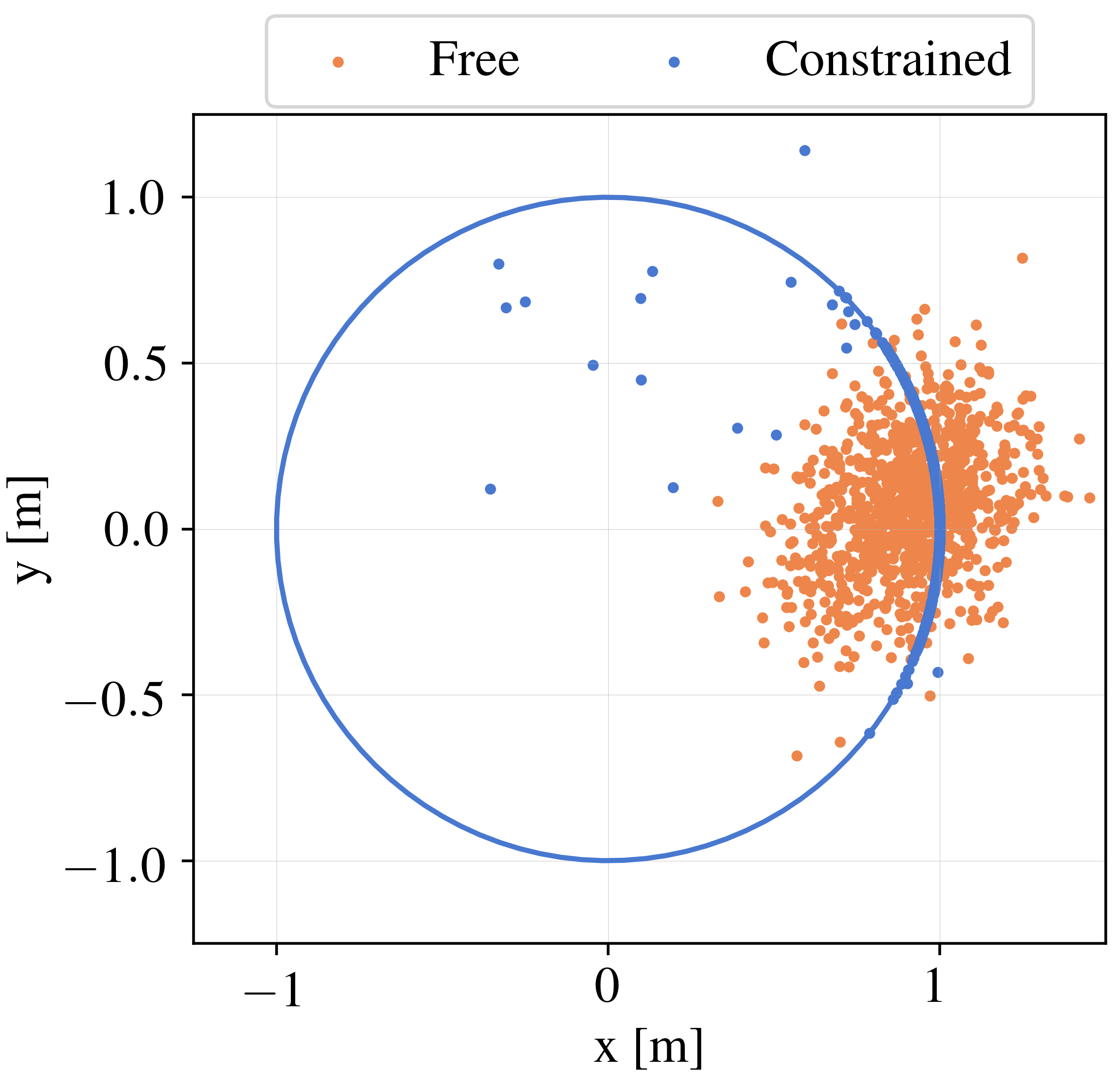
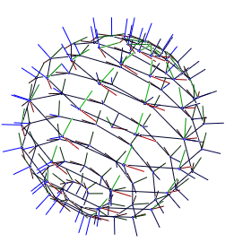
(a)	(b)

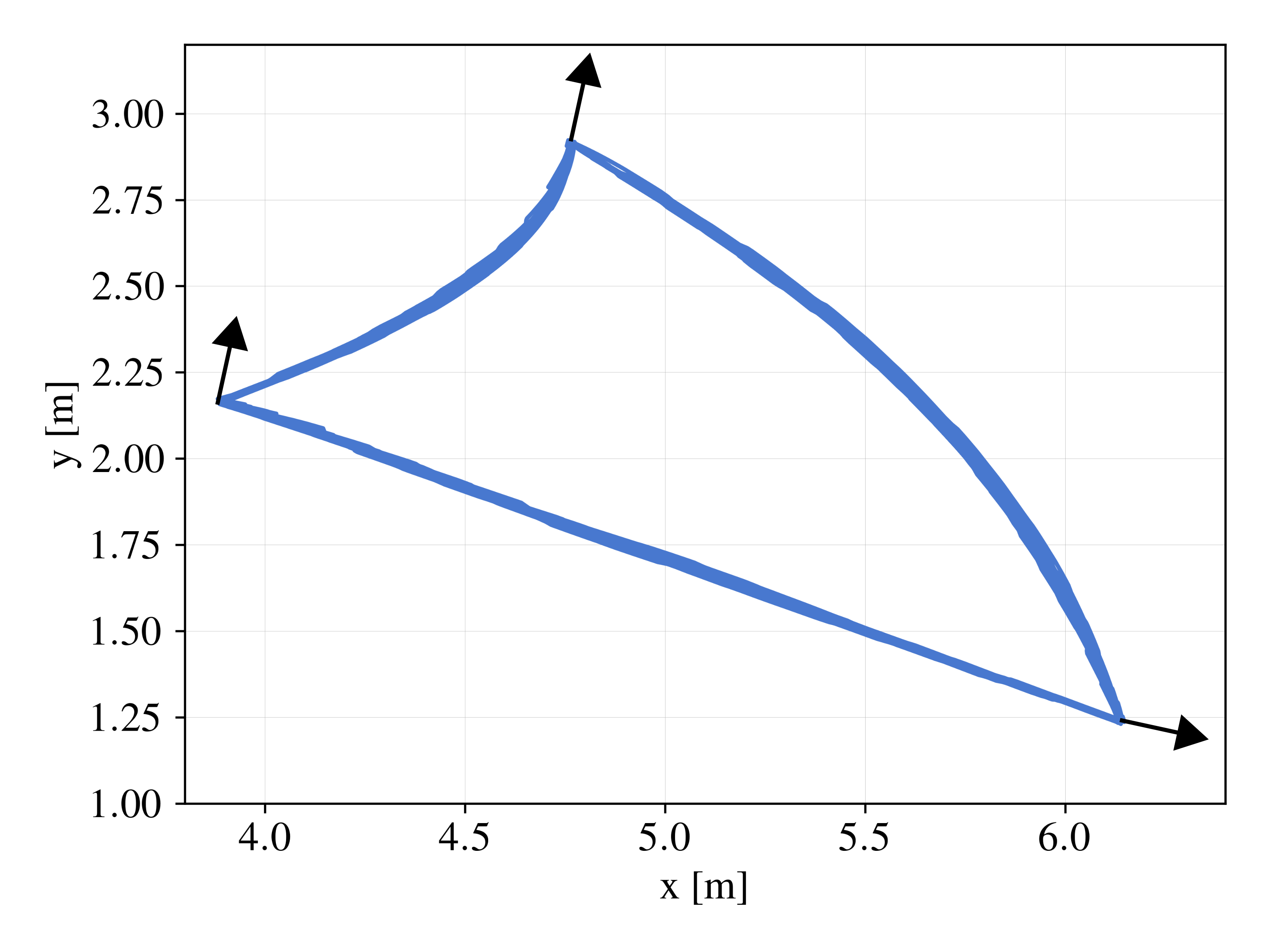
(c)

Figure 1: Three application studies: (a) pose estimation; (b) rotation synchronization; (c) MPC of a pseudo-onidirectional platform; the robot is traveling across three goals, with desired orientation represented by the arrows.

The core idea of our method is to use the AL method to model a new type of factors which can be directly included in existing unconstrained solvers: the constraint factors. Handling constraints enlarges the application domain of factor graphs confirming them as a general framework for optimization in robotics.

In this paper, we first review the theoretical bases and subsequently present an algorithm scheme that might be used as reference implementation. We cast this algorithm to three increasingly complex problems, which are shown in Fig. 1. The first is pose estimation of a unicycle, subject to the constraint that the estimate is coherent with the kinematics model. In this example the robot starts in the origin and applies only linear velocity, therefore it is known to lye on the circumference independently from the initial unknown orientation. The second is rotation synchronization [eriksson2021tpa] subject to the constraint that the estimate is actually a rotation matrix. The system can recover orientations of the poses from arbitrary initial guesses. The third is MPC of the pseudo-omnidirectional platform presented in [andreasson2022mdpi], which comprises dynamics, velocity and acceleration constraints. In introducing each application, we provide the reader with practical insights on implementation and parameter choices. With these three examples, we show that using constrained factor graphs and AL can produce results that compare favorably against domain specific approaches.

II Related Work

Factor graphs optimization is a very powerful tool to compute optimal solutions to many problems in robotics [dellaert2021ar]. Factor graph solvers exploit the sparsity pattern for efficiency. They address nonlinear unconstrained optimization problems using ILS [grisetti2020solver]. Extending factor graphs to constrained optimization is a relevant topic: it allows both new ways of addressing old problems, such as distributed or robust SLAM [cunningham2015icra, choudhary2015icra, bai2018iros], and new applications of the tool, such as Optimal Control [xie2020corr, sodhi2020icra, qadri2022incopt].

Choudhary et al. [choudhary2015iros] address the problem of memory efficiency in SLAM by splitting the graph into sub-graphs and imposing consistency of the separators using hard constraints. The resulting optimization problem is solved in a decentralized manner using the multi-block Alternating Direction Method of Multipliers (ADMM) [boyd2011ml]. Differently, Cunningham et al. [cunningham2010iros] use Gram-Schmidt orthogonalization for elimination of the constrained variables when solving linear constrained sub-problems. In order to boost robustness against local minima in SLAM, Bai et al. [bai2018iros] represent loop closures as constraints and use Iterative Sequential Quadratic Programming (iSQP) to solve the resulting constrained SLAM graphs.

The versatility of factor graphs was exploited to address motion planning problems [dong2016rss, mukadam2019ar] which increased the interest in constraints-embedding factor graphs. Yang et al. [yang2021icra] propose to devolve the solution of the constrained optimization problem for variable elimination to a specialized solver. They then focus on the Linear Quadratic Regulator problem, where the constrained sub-problem can be trivially solved. The difference with our method is that our factor graph-solver embeds general constraints, without the need of relying on a specialized solver. Also iSQP was investigated as a method to embed nonlinear constraints in factor graph-based estimation and MPC on Unmanned Aerial Vehicles by Ta et al. [ta2014icuas]. Finally, Xie et al. [xie2020corr] convert the constrained problem into an unconstrained one by introducing a loss function for each constraint. They present motion planning applications ranging from cart-pole to quadruped robots.

Orthogonal to [xie2020corr, ta2014icuas], the method proposed by Sodhi et al. [sodhi2020icra] leverages on the AL method to extend the incremental smoothing solver by Kaess et al. [kaess2008tro] with constraints-handling. They explain how to represent constrained optimization over a Bayes Tree. More recently, the newer version of the solver was presented by Qadri et al. [qadri2022incopt] where online relinearization is used for efficiency. In the computer vision literature, the AL method was adopted by Eriksson et al. [eriksson2021tpa] to address the rotation synchronization problem. We present it here as well, with a focus on its embedding in our framework.

Inspired by [sodhi2020icra, qadri2022incopt], this work revisits AL on factor graphs and provides an implementation scheme of our primal-dual procedure. We test its generality with application to three problems from different areas and of varying complexity. The MPC application is supported with real-world experiments. Moreover, we comment on the adaptation schemes used for the main parameters. This work builds on our previous work [bazzana2023ral] and generalizes its ideas, including general nonlinear constraints in the formulation. Finally, we here propose a different AL function from the one previously used in the literature of factor graphs, and compare the two.

III Our Approach

In this paper we present an extension of ILS on factor graphs to solve NonLinear Programming (NLP) using the AL method. Factor graphs are bipartite graphs with two kinds of nodes: variables and factors. Variables represent the state of our system, while factor nodes model dependence relationships between the neighbor variables.

Let $\mathbf{x}=\mathbf{x}_{0:N-1}$ be the set of all variables which can span over arbitrary continuous domains, with $\mathbf{x}_{n}$ element of a manifold [hertzberg2013sd], e.g. the special Euclidean group $\mathrm{SE}(3)$. Let us represent the $k^{\mathrm{th}}$ factor as $\left<\mathbf{\Omega}_{k},\mathbf{e}_{k}(\cdot)\right>$ with $\mathbf{e}_{k}\in\mathbb{R}^{z}$ representing the difference between predicted and actual $k^{\mathrm{th}}$ measurement with information matrix $\mathbf{\Omega}_{k}\in\mathbb{R}^{z\times z}$, only depending on the subset of variables $\mathbf{x}^{k}=\mathbf{x}_{k_{0}:k_{K}}$. A factor graph models the summation

$$F(\mathbf{x})=\sum_{k=0}^{K-1}||\mathbf{e}_{k}(\mathbf{x}^{k})||_{\mathbf{\Omega}_{k}}^{2}$$ (1)

where $||\mathbf{e}_{k}(\mathbf{x}^{k})||_{\mathbf{\Omega}_{k}}^{2}=\mathbf{e}_{k}(\mathbf{x}^{k})^{T}\mathbf{\Omega}_{k}\mathbf{e}_{k}(\mathbf{x}^{k})$. Under Gaussian assumptions,  Eq. (1) expresses the negative log-likelihood of the measurements given the states. Factor graph-solvers compute the variables $\mathbf{x}$ which minimize Eq. (1), using the ILS approach [grisetti2020solver]. At each iteration, the current solution $\hat{\mathbf{x}}$ is refined by taking a Gauss-Newton step over Eq. (1): $\hat{\mathbf{x}}\leftarrow\hat{\mathbf{x}}\boxplus\mathbf{\Delta x}$; where $\mathbf{H}\mathbf{\Delta x}=-\mathbf{b}$, and $\boxplus$ adds the Euclidean perturbation $\mathbf{\Delta x}$ to $\hat{\mathbf{x}}$ in the manifold space. By using the first order Taylor expansion of the error function $\mathbf{e}_{k}(\hat{\mathbf{x}}\boxplus\mathbf{\Delta}\mathbf{x})\simeq\hat{\mathbf{e}}_{k}+\mathbf{J}_{k}\mathbf{\Delta}\mathbf{x}$ around $\hat{\mathbf{x}}$ in Eq. (1), we get

$$\mathbf{b}=\sum_{k=0}^{K-1}\overbrace{\mathbf{J}_{k}^{T}\mathbf{\Omega}_{k}\hat{\mathbf{e}}_{k}}^{\mathbf{b}^{k}}\qquad\mathbf{H}=\sum_{k=0}^{K-1}\overbrace{\mathbf{J}_{k}^{T}\mathbf{\Omega}_{k}\mathbf{J}_{k}}^{\mathbf{H}^{k}}$$ (2)

III-A Augmented Lagrangian for Nonlinear Programming

Consider the following NLP problem

$$\mathbf{x}^{*}=\mathop{\operatorname*{argmin}}\limits_{\mathbf{x}}\overbrace{\sum_{k=0}^{K-1}||\mathbf{e}_{k}(\mathbf{x}^{k})||_{\mathbf{\Omega}_{k}}^{2}}^{F(\mathbf{x})},$$ (3)

$$\mathrm{subject\,to}\, \mathbf{f}_{{k_{\mathrm{f}}}}(\mathbf{x}^{{k_{\mathrm{f}}}})=\mathbf{0},\,{k_{\mathrm{f}}}=0,...,K_{\mathrm{f}}-1,$$

$$\mathbf{g}_{{k_{\mathrm{g}}}}(\mathbf{x}^{{k_{\mathrm{g}}}})\leq\mathbf{0},\,{k_{\mathrm{g}}}=0,...,K_{\mathrm{g}}-1$$

with $K_{\mathrm{f}}$ multidimensional equality constraints $\mathbf{f}_{k_{f}}(\cdot)$ and $K_{\mathrm{g}}$ multidimensional inequality constraints $\mathbf{g}_{{k_{\mathrm{g}}}}(\cdot)$, only involving a subset of variables, respectively $\mathbf{x}^{{k_{\mathrm{f}}}}$ and $\mathbf{x}^{{k_{\mathrm{g}}}}$. Eq. (3) can be converted into an equality constrained problem by introducing $K_{\mathrm{g}}$ vectors of the type $\mathbf{q}_{{k_{\mathrm{g}}}}=(q_{0}\,,q_{1}\,,\,...,\,q_{{k_{\mathrm{g}}},J-1})^{T}$ with $q_{i}>0,\,\forall\,i=0,1,...,{k_{\mathrm{g}}},J-1$, one for each inequality constraint $\mathbf{g}_{{k_{\mathrm{g}}}}(\cdot)$ of dimension ${k_{\mathrm{g}}},J$

$$\mathbf{x}^{*}=\mathop{\operatorname*{argmin}}\limits_{\mathbf{x}}\overbrace{\sum_{k=0}^{K-1}||\mathbf{e}_{k}(\mathbf{x}_{k})||_{\mathbf{\Omega}_{k}}^{2}}^{F(\mathbf{x})},$$ (4)

$$\mathrm{subject\,to}\, \mathbf{f}_{{k_{\mathrm{f}}}}(\mathbf{x}^{{k_{\mathrm{f}}}})=\mathbf{0},\,{k_{\mathrm{f}}}=0,...,K_{\mathrm{f}}-1,$$

$$\mathbf{g}_{{k_{\mathrm{g}}}}(\mathbf{x}^{{k_{\mathrm{g}}}})+\mathbf{q}_{{k_{\mathrm{g}}}}=\mathbf{0},\,{k_{\mathrm{g}}}=0,...,K_{\mathrm{g}}-1$$

Algorithm 1 Augmented Lagrangian-Iterative Least Squares

$\left<\mathbf{\Omega}_{k},\mathbf{e}_{k}(\cdot)\right>_{0:K-1}$, error factors

$\left<\boldsymbol{\lambda}^{k},\mathbf{P}_{k_{\mathrm{f}}},\mathbf{f}_{k_{\mathrm{f}}}(\cdot)\right>_{0:K_{\mathrm{f}}-1}$, equality constraint factors

$\left<\boldsymbol{\mu}^{k},\mathbf{P}_{k_{\mathrm{g}}},\mathbf{g}_{k_{\mathrm{g}}}(\cdot)\right>_{0:K_{\mathrm{g}}-1}$, inequality constraint factors

$I_{\mathrm{GN}}$, number of inner Gauss-Newton (GN) iterations

while !converged do

     for $I_{\mathrm{GN}}$ do

         $\mathbf{H}\leftarrow\mathbf{0}$

         $\mathbf{b}\leftarrow\mathbf{0}$

         for all factors do

              $\mathbf{b}~{}\mathrel{+}=\mathbf{b}^{k},\,\mathbf{H}~{}\mathrel{+}=\mathbf{H}^{k}$ (Eq. (2))

              $\mathbf{b}~{}\mathrel{+}=\mathbf{b}^{k_{\mathrm{f}}},\,\mathbf{H}~{}\mathrel{+}=\mathbf{H}^{k_{\mathrm{f}}}$ (Eq. (11))

              $\mathbf{b}~{}\mathrel{+}=\mathbf{b}^{k_{\mathrm{g}}},\,\mathbf{H}~{}\mathrel{+}=\mathbf{H}^{k_{\mathrm{g}}}$ (Eq. (11))          

         $\mathbf{\Delta x}\leftarrow\mathrm{solve}(\mathbf{H}\mathbf{\Delta x}=-\mathbf{b})$

         $\hat{\mathbf{x}}\leftarrow\hat{\mathbf{x}}\boxplus\mathbf{\Delta x}$      

     for all constraint factors do

         $\boldsymbol{\lambda}^{k_{\mathrm{f}}}\leftarrow\boldsymbol{\lambda}^{k_{\mathrm{f}}}+2\mathbf{P}_{{k_{\mathrm{f}}}}\mathbf{f}_{k_{\mathrm{f}}}(\mathbf{x}^{k_{\mathrm{f}}})$ (Eq. (12))

         $\boldsymbol{\mu}^{k_{\mathrm{g}}}\leftarrow\max(\mathbf{0},\boldsymbol{\mu}^{k_{\mathrm{g}}}+2\mathbf{P}_{{k_{\mathrm{g}}}}\mathbf{g}_{k_{\mathrm{g}}}(\mathbf{x}^{k_{\mathrm{g}}}))$ (Eq. (12))

         Update $\rho$ (Eq. (13))      

Hence, the Augmented Lagrangian for problem Eq. (3) becomes

$$\mathcal{L}(\mathbf{x},\mathbf{q};\boldsymbol{\lambda},\boldsymbol{\mu},\mathbf{P})=F(\mathbf{x})$$ (5)

$$+\sum_{{k_{\mathrm{f}}}=0}^{K_{\mathrm{f}}-1}\big{[}{\boldsymbol{\lambda}^{{k_{\mathrm{f}}}}}^{T}\mathbf{f}_{{k_{\mathrm{f}}}}(\mathbf{x}^{{k_{\mathrm{f}}}})+|\mathbf{f}_{{k_{\mathrm{f}}}}(\mathbf{x}^{{k_{\mathrm{f}}}})||_{\mathbf{P}_{{k_{\mathrm{f}}}}}^{2}\big{]}$$

$$+\sum_{{k_{\mathrm{g}}}=0}^{K_{\mathrm{g}}-1}\big{[}{\boldsymbol{\mu}^{k_{\mathrm{g}}}}^{T}(\mathbf{g}_{k_{\mathrm{g}}}(\mathbf{x}^{k_{\mathrm{g}}})+\mathbf{q}_{k_{\mathrm{g}}})+||\mathbf{g}_{k_{\mathrm{g}}}(\mathbf{x}^{k_{\mathrm{g}}})+\mathbf{q}_{k_{\mathrm{g}}}||^{2}_{\mathbf{P}_{{k_{\mathrm{g}}}}}\big{]}$$

Differently from [bertsekas2014ap], we use here diagonal matrices $\mathbf{P}_{{k_{\mathrm{f}}}}=\mathrm{diag}(\rho_{{k_{\mathrm{f}}},1},\rho_{{k_{\mathrm{f}}},2},...,\rho_{{k_{\mathrm{f}}},j})$ and $\mathbf{P}_{{k_{\mathrm{g}}}}=\mathrm{diag}(\rho_{{k_{\mathrm{g}}},1},\rho_{{k_{\mathrm{g}}},2},...,\rho_{{k_{\mathrm{g}}},j})$, as big as the dimension of the constraints, instead of two scalar penalties $\rho_{{k_{\mathrm{f}}}}$ and $\rho_{{k_{\mathrm{g}}}}$. In this way, every component of the constraints is weighted by a different coefficient, which can be adapted based on the magnitude of the constraint violation along the corresponding dimension, rather than on the overall norm.

The Lagrangian method [bertsekas2014ap] iteratively minimizes Eq. (5) with respect to $(\mathbf{x},\mathbf{q})$ for various values of $(\boldsymbol{\lambda},\boldsymbol{\mu},\mathbf{P})$. If $\mathbf{x}$ and $(\boldsymbol{\lambda},\boldsymbol{\mu},\mathbf{P})$ are fixed, $\mathcal{L}(\mathbf{x},\mathbf{q};\boldsymbol{\lambda},\boldsymbol{\mu},\mathbf{P})$ in Eq. (5) can be minimized with respect to $\mathbf{q}$. Furthermore, considering $\mathbf{P}_{k_{\mathrm{g}}}$ diagonal makes the minimization in each component $q_{i}$ of $\mathbf{q}_{k_{\mathrm{g}}}$ independent

$$q_{i}^{*}=\operatorname*{argmin}_{{q_{i}}>0}{{\mu_{{k_{\mathrm{g}}},i}}(g_{{k_{\mathrm{g}}},i}(\mathbf{x}^{k_{\mathrm{g}}})+{q_{i}})+\rho_{{k_{\mathrm{g}}},i}(g_{{k_{\mathrm{g}}},i}(\mathbf{x}^{k_{\mathrm{g}}})+q_{i})^{2}}$$ (6)

Eq. (6) is a quadratic function in $q_{i}$, with unconstrained minimum $\hat{q}_{i}=-\left[\frac{\mu_{{k_{\mathrm{g}}},i}}{2\rho_{{k_{\mathrm{g}}},i}}+g_{{k_{\mathrm{g}}},i}(\mathbf{x}^{k_{\mathrm{g}}})\right]$. Its global minimum subject to ${q_{i}}>0$ is therefore

$${q_{i}}^{*}=\max\left(0,-\left[\frac{\mu_{{k_{\mathrm{g}}},i}}{2\rho_{{k_{\mathrm{g}}},i}}+g_{{k_{\mathrm{g}}},i}(\mathbf{x}^{k_{\mathrm{g}}})\right]\right)$$ (7)

Let $\mathbf{g}_{{k_{\mathrm{g}}}}^{+}(\mathbf{x}^{k_{\mathrm{g}}})=\mathbf{g}_{{k_{\mathrm{g}}}}(\mathbf{x}^{k_{\mathrm{g}}})+\mathbf{q}_{{k_{\mathrm{g}}}}^{*}$, component-wise

$$g_{{k_{\mathrm{g}}},i}^{+}(\mathbf{x}^{k_{\mathrm{g}}})=g_{{k_{\mathrm{g}}},i}(\mathbf{x}^{k_{\mathrm{g}}})+q_{i}^{*}=\max\left(g_{{k_{\mathrm{g}}},i}(\mathbf{x}^{k_{\mathrm{g}}}),-\frac{\mu_{{k_{\mathrm{g}}},i}}{2\rho_{{k_{\mathrm{g}}},i}}\right)$$ (8)

the Augmented Lagrangian for problem Eq. (3) can be finally written as

$$\mathcal{L}(\mathbf{x},\mathbf{q};\boldsymbol{\lambda},\boldsymbol{\mu},\mathbf{P})=\sum_{k=0}^{K-1}||\mathbf{e}_{k}(\mathbf{x}^{k})||^{2}_{\mathbf{\Omega}_{k}}$$ (9)

$$+\sum_{{k_{\mathrm{f}}}=0}^{K_{\mathrm{f}}-1}\big{[}{\boldsymbol{\lambda}^{{k_{\mathrm{f}}}}}^{T}\mathbf{f}_{{k_{\mathrm{f}}}}(\mathbf{x}^{{k_{\mathrm{f}}}})+||\mathbf{f}_{{k_{\mathrm{f}}}}(\mathbf{x}^{{k_{\mathrm{f}}}})||_{\mathbf{P}_{{k_{\mathrm{f}}}}}^{2}\big{]}$$

$$+\sum_{{k_{\mathrm{g}}}=0}^{K_{\mathrm{g}}-1}\big{[}{\boldsymbol{\mu}^{k_{\mathrm{g}}}}^{T}\mathbf{g}_{k_{\mathrm{g}}}^{+}(\mathbf{x}^{k_{\mathrm{g}}})+||\mathbf{g}_{k_{\mathrm{g}}}^{+}(\mathbf{x}^{k_{\mathrm{g}}})||^{2}_{\mathbf{P}_{{k_{\mathrm{g}}}}}\big{]}$$

Each term in parenthesis can be modeled as a factor in a factor-graph. In the next section, we specify how factors corresponding to constraints differ from regular error factors of classical ILS solvers.

III-B Augmented Lagrangian on Factor Graphs

The AL method [bertsekas2014ap] is a primal-dual method for solving Eq. (3) which computes the solution to the $\mathrm{maxmin}$ dual problem $\mathrm{max_{\boldsymbol{\lambda},\boldsymbol{\mu}}min_{\mathbf{x}}}\mathcal{L}(\mathbf{x},\boldsymbol{\lambda},\boldsymbol{\mu})$. At each iteration $i$, the primal step updates $\mathbf{x}$ by minimizing $\mathcal{L}(\mathbf{x},\boldsymbol{\lambda},\boldsymbol{\mu})$ with fixed $(\boldsymbol{\lambda},\boldsymbol{\mu})$. Our solver updates the current estimate of $\mathbf{x}$ by taking $I_{\mathrm{GN}}$ Gauss-Newton steps over the AL function of Eq. (9). The quadratic approximation of Eq. (9) is computed considering the first-order Taylor expansion of the error function and of the constraints around the current estimate $\hat{\mathbf{x}}$

$$\mathbf{e}_{k}(\hat{\mathbf{x}}^{k}\boxplus\mathbf{\Delta}\mathbf{x}^{k}) \simeq\hat{\mathbf{e}}_{k}+\mathbf{J}_{k}\mathbf{\Delta}\mathbf{x}^{k}$$ (10)

$$\mathbf{f}_{k_{\mathrm{f}}}(\hat{\mathbf{x}}^{k_{\mathrm{f}}}\boxplus\mathbf{\Delta}\mathbf{x}^{k_{\mathrm{f}}}) \simeq\hat{\mathbf{f}}_{k_{\mathrm{f}}}+\mathbf{F}_{k_{\mathrm{f}}}\mathbf{\Delta}\mathbf{x}^{k_{\mathrm{f}}}$$

$$\mathbf{g}_{k_{\mathrm{g}}}^{+}(\hat{\mathbf{x}}^{k_{\mathrm{g}}}\boxplus\mathbf{\Delta}\mathbf{x}^{k_{\mathrm{g}}}) \simeq\hat{\mathbf{g}}^{+}_{k_{\mathrm{g}}}+\mathbf{G}^{+}_{k_{\mathrm{g}}}\mathbf{\Delta}\mathbf{x}^{k_{\mathrm{g}}}$$

Using the $\boxplus$ operator on the state manifold, the estimate is updated according to $\hat{\mathbf{x}}\leftarrow\hat{\mathbf{x}}\boxplus\mathbf{\Delta x}$, where $\mathbf{H}^{L}\mathbf{\Delta x}=-\mathbf{b}^{L}$:

$$\mathbf{b}^{L} =\mathbf{b}+\sum_{{k_{\mathrm{f}}}=0}^{K_{\mathrm{f}}-1}\overbrace{\mathbf{F}_{k_{\mathrm{f}}}^{T}\mathbf{P}_{{k_{\mathrm{f}}}}\hat{\mathbf{f}}_{k_{\mathrm{f}}}\!+\!\frac{1}{2}{\mathbf{F}_{k_{\mathrm{f}}}}^{T}\boldsymbol{\lambda}^{k_{\mathrm{f}}}}^{\mathbf{b}^{k_{\mathrm{f}}}}$$ (11)

$$+\sum_{{k_{\mathrm{g}}}=0}^{K_{\mathrm{g}}-1}\overbrace{{\mathbf{G}^{+}_{k_{\mathrm{g}}}}^{T}\mathbf{P}_{{k_{\mathrm{g}}}}\hat{\mathbf{g}}^{+}_{k_{\mathrm{g}}}\!+\!\frac{1}{2}{\mathbf{G}^{+}_{k_{\mathrm{g}}}}^{T}\boldsymbol{\mu}^{k_{\mathrm{g}}}}^{\mathbf{b}^{k_{\mathrm{g}}}}$$

$$\mathbf{H}^{L} =\mathbf{H}+\sum_{{k_{\mathrm{f}}}=0}^{K_{\mathrm{f}}-1}\overbrace{\mathbf{F}_{k_{\mathrm{f}}}^{T}\mathbf{P}_{{k_{\mathrm{f}}}}\mathbf{F}_{k_{\mathrm{f}}}}^{\mathbf{H}^{k_{\mathrm{f}}}}+\sum_{{k_{\mathrm{g}}}=0}^{K_{\mathrm{g}}-1}\overbrace{{\mathbf{G}^{+}_{k_{\mathrm{g}}}}^{T}\mathbf{P}_{{k_{\mathrm{g}}}}\mathbf{G}^{+}_{k_{\mathrm{g}}}}^{\mathbf{H}^{k_{\mathrm{g}}}}.$$

with $\mathbf{H}$ and $\mathbf{b}$ from Eq. (2). Hence, ${k_{\mathrm{f}}}$-th and ${k_{\mathrm{g}}}$-th constraint factors contribute to $\mathbf{H}^{L}$ and $\mathbf{b}^{L}$, respectively with $\mathbf{H}^{{k_{\mathrm{f}}}},\mathbf{b}^{k_{\mathrm{f}}}$ and $\mathbf{H}^{{k_{\mathrm{g}}}},\mathbf{b}^{k_{\mathrm{g}}}$.

The dual step happens within the constraint factors where $(\boldsymbol{\lambda},\boldsymbol{\mu})$ are updated by taking projected gradient ascent step over $\mathcal{L}(\mathbf{x},\boldsymbol{\lambda},\boldsymbol{\mu})$ with fixed $\mathbf{x}$ weighted by the penalty coefficients $\mathbf{P}_{\mathbf{f}},\mathbf{P}_{\mathbf{g}}$

$$\begin{cases}\boldsymbol{\lambda}^{k_{\mathrm{f}}}\leftarrow\boldsymbol{\lambda}^{k_{\mathrm{f}}}+2\,\mathbf{P}_{{k_{\mathrm{f}}}}\mathbf{f}_{k_{\mathrm{f}}}(\mathbf{x}^{k_{\mathrm{f}}}),\,{k_{\mathrm{f}}}=0,...,{K_{\mathrm{f}}-1}\\ \boldsymbol{\mu}^{k_{\mathrm{g}}}\leftarrow\max(\mathbf{0},\boldsymbol{\mu}^{k_{\mathrm{g}}}+2\,\mathbf{P}_{{k_{\mathrm{g}}}}\mathbf{g}_{k_{\mathrm{g}}}(\mathbf{x}^{k_{\mathrm{g}}})),\,{k_{\mathrm{g}}}=0,...,{K_{\mathrm{g}}-1}\end{cases}$$ (12)

Penalty parameters in $\mathbf{P}_{{k_{\mathrm{f}}}}$ and $\mathbf{P}_{{k_{\mathrm{g}}}}$ are usually adapted based on the evolution of the constraint violation between subsequent iterations [sodhi2020icra].

In the following, we present the adaptation scheme we used. Let us denote as $\rho$ the coefficient associated to the constraint $\mathbf{f}=0$, as $\mathbf{f}^{-}=\mathrm{max}(0,|\mathbf{f}_{i-1}|-|\mathbf{f}_{i}|/|\mathbf{f}_{i-1}|)$ the percentage decrease in constraint violation from iteration $i-1$ to iteration $i$, and as $\mathbf{f}^{+}=\mathrm{max}(0,(|\mathbf{f}_{i}|-|\mathbf{f}_{i-1}|)/|\mathbf{f}_{i}|)$ the percentage increase in constraint violation. At iteration $i$, our choice is to compute $\rho$ in the range $(\rho_{\mathrm{m}},\bar{\rho})$ if $\mathbf{f}^{+}$ is positive, or $(\bar{\rho},\rho_{\mathrm{M}})$ if $\mathbf{f}^{-}$ is positive

$$\begin{cases}\rho=\bar{\rho}_{i}+\mathbf{f}^{-}(\rho_{\mathrm{M}}-\bar{\rho}_{i})+\mathbf{f}^{+}(\rho_{\mathrm{m}}-\bar{\rho}_{i})\\ \bar{\rho}_{i+1}=\bar{\rho}_{i}+\mathbf{f}^{-}(\rho_{\mathrm{M}}-\bar{\rho}_{i}).\end{cases}$$ (13)

$\bar{\rho}$ changes over the iterations to guarantee that the increase in $\rho$ due to reduction in constraint violation is kept across subsequent iterations. Otherwise, constant constraint violation would result in decreasing $\rho$. Clamping $\rho$ within the interval $(\rho_{\mathrm{m}},\rho_{\mathrm{M}})$ prevents the algorithm from diverging in case of bad initial guesses, while allowing larger values to be used when constraint satisfaction is improving. In all practical applications described in the remainder, we use $\bar{\rho}_{0}=1.0,\rho_{\mathrm{m}}=0.5,\rho_{\mathrm{M}}=2.0$. Further, all Lagrange Multipliers are initialized at zero in the applications.

IV Applications

The objective of this work is to present a methodology to address general constrained optimization problems using factor graphs. In the following we present three applications to show the capabilities of our approach: (i) improve in performance thanks to inclusion of constraints in pose estimation; (ii) alternative approach to rotation synchronization which directly includes rotation matrix constraints; (iii) runtime advantage compared to Interior Point OPTimizer (IPOPT) in MPC.

IV-A Constrained Pose Estimation

2D pose estimation is the problem of determining robot position and heading $\mathbf{X}^{W}_{R}=[\mathbf{t};\,\theta]=[x,\,y,\,\theta]\in\mathrm{SE}(2)$ that maximize the likelihood of the measurements. As an illustrative example of how the capacity of handling constraints can improve the performance, we address here the 2D navigation application of Barrau et al.[barrau2020tac]. A unicycle starts from perfectly known position $\mathbf{t}=[0,0]^{T}$ with unknown heading. It drives in straight line with constant linear velocity $v$ and zero angular velocity $\omega$ for known time $\mathrm{T}$. It then receives a GPS measurement of its new position $\mathbf{z}_{\mathrm{GPS}}\in\mathbb{R}^{2}$, and uses it to correct the odometry measurement $\mathbf{Z}_{\mathrm{ODOM}}=[\mathbf{t}_{\mathrm{ODOM}};\,\theta_{\mathrm{ODOM}}]\in\mathrm{SE}(2)$, obtained integrating the unicycle kinematics from the initial guess $\mathbf{X}^{W}_{R,\mathrm{ig}}=[0,0,\theta_{0}]$. Fig. 3 illustrates the problem assuming $v=1\mathrm{m/s}$, $\mathrm{T}=1\mathrm{s}$ and zero ground-truth orientation (orange triangles).

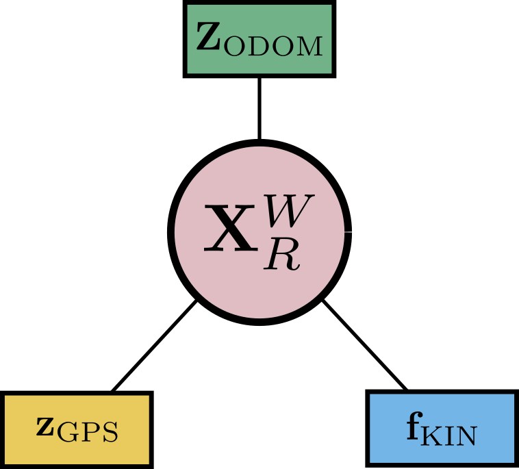
Figure 2: Factor graph modeling the pose estimation problem subject to kinematics which constrains the pose on a circumference with radial orientation.

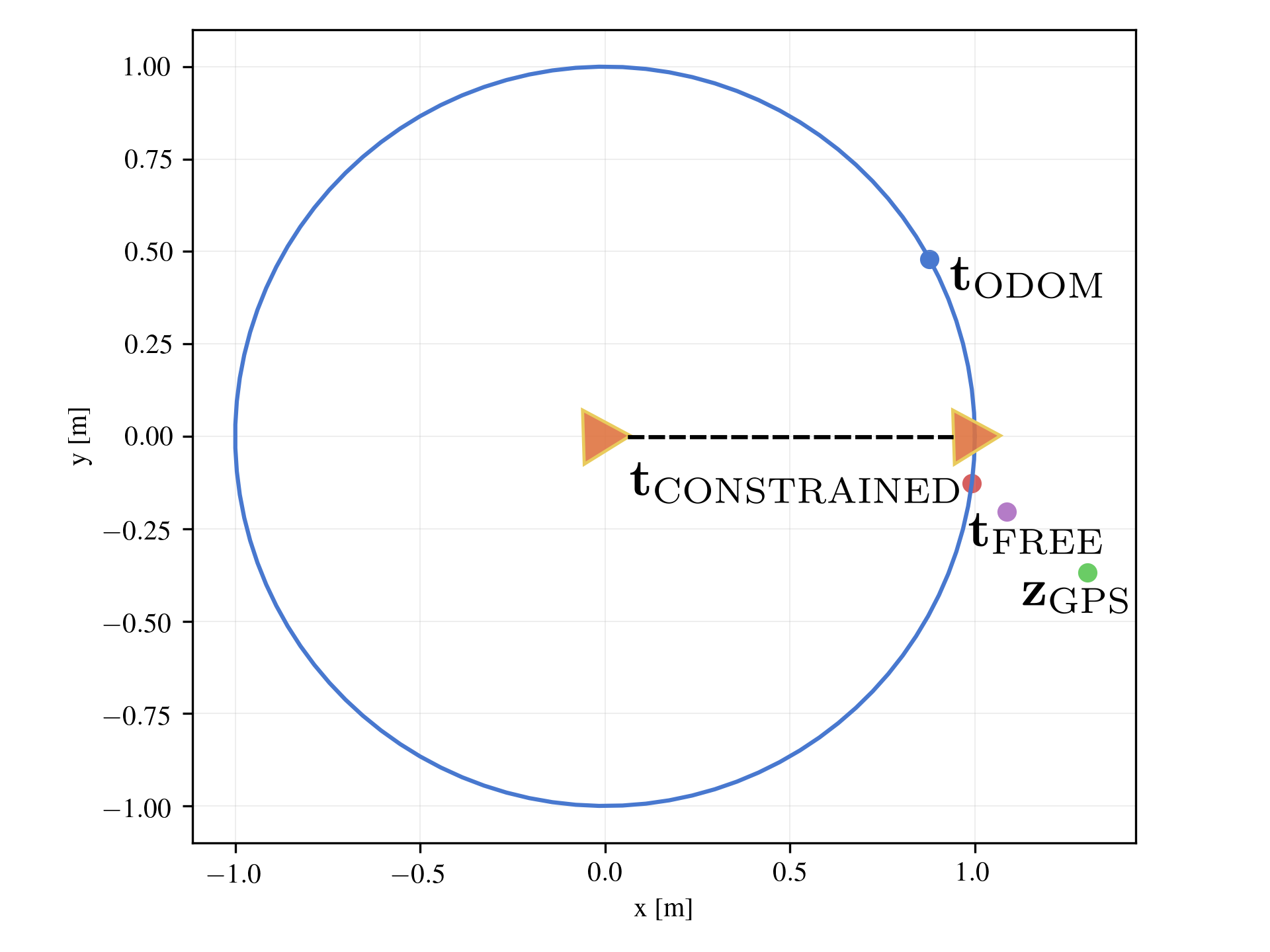
Figure 3: Representation of the constrained estimation problem. By adding the constraint Eq. (15) to the optimization problem, $\mathbf{t}_{\mathrm{CONSTRAINED}}$ is closer to Ground Truth $[1,0,0]$ compared to $\mathbf{t}_{\mathrm{FREE}}$.

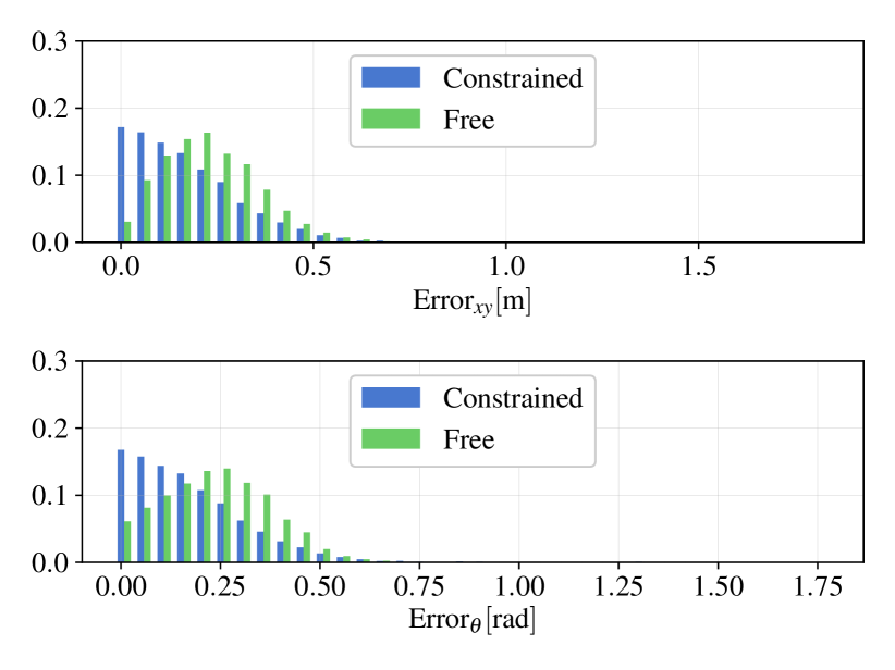
Figure 4: Probability distribution of linear and rotational error of the estimate with and without the constraint of Eq. (15). Each test corresponds to a different $\mathbf{z}_{\mathrm{GPS}}$ extracted from the normal distribution $\mathcal{N}([1,0,0];\mathbf{\Omega}_{\mathrm{GPS}})$, with $\theta_{0}=0.5\mathrm{rad}$.

Traditionally, the estimate of the robot pose $\mathbf{X}^{W}_{R}$ is obtained by solving

$$F(\mathbf{X}^{W}_{R})=||\mathbf{t}-\mathbf{z}_{\mathrm{GPS}}||_{\mathbf{\Omega}_{\mathrm{GPS}}}^{2}+||{\mathbf{X}^{W}_{R}}^{-1}\mathbf{Z}_{\mathrm{ODOM}}||_{\mathbf{\Omega}_{\mathrm{ODOM}}}^{2}$$ (14)

It finds the estimate which best explains both odometry and GPS measurements. However, it neglects the information that the robot is moving on a straight line, which implies (a) robot position on the circumference (b) the heading $[\cos(\theta),\sin(\theta)]^{T}$ is radial. The two conditions are summarized by

$$\mathbf{f}_{\mathrm{KIN}}(\mathbf{X})=\begin{pmatrix}x^{2}+y^{2}-(v\mathrm{T})^{2}\\ x\sin(\theta)-y\cos(\theta)\end{pmatrix}=\begin{pmatrix}0\\ 0\end{pmatrix}$$ (15)

The constraint factor modeling Eq. (15) is represented by the blue square in Fig. 2. As any other factor, it is connected to the variable on which it depends. Fig. 4 shows the probability distribution of the translational and rotational error obtained over 10K experiments with $\mathbf{\Omega}_{\mathrm{ODOM}}=10\,\mathbf{I}_{3\times 3}$ and $\mathbf{\Omega}_{\mathrm{GPS}}=20\,\mathbf{I}_{3\times 3}$. Lower errors are more likely imposing Eq. (15).

IV-B Rotation Synchronization

The second application we consider is Rotation Synchronization in $\mathbb{R}^{3}$ [eriksson2021tpa]. It is the $\mathrm{SO}(3)$ instance of the Group Synchronization problem which consists in finding the elements of a group, in our case $\mathbf{R}_{i}\in\mathbb{R}^{3\times 3}$ with $\mathbf{R}_{i}^{T}\mathbf{R}_{i}=\mathbf{I}_{3\times 3};\,\det\mathbf{R}_{i}=1$, starting from pairwise measurements $\mathbf{Z}^{i}_{j}$, in our case $\mathbf{R}_{i}^{T}\mathbf{R}_{j}$. It is a sub-problem of many applications from SfM to pose graph optimization. In absence of a good initial guess, a solution is obtained by finding a set of matrices $\mathbf{A}\in\mathbb{R}^{3\times 3}$ that minimize

$$F(\mathbf{A}_{0:n})=\sum_{i,j}||\mathrm{flatten}(\mathbf{A}_{i}\mathbf{Z}^{i}_{j}-\mathbf{A}_{j})||_{\mathbf{\Omega}_{i,j}}^{2}$$ (16)

where the operator $\mathrm{flatten}(\cdot):\mathbb{R}^{3\times 3}\leftarrow\mathbb{R}^{9}$ stacks the rows of the input matrix into a vector. Once a solution is found, the closest rotation matrices $\mathbf{R}^{*}_{0:n}$ are obtained by Singular Value Decomposition (SVD)

$$\mathbf{R}^{*}_{i}=\mathbf{U}_{i}^{T}\mathbf{V}_{i}\leftarrow\mathbf{U}_{i},\mathbf{S}_{i},\mathbf{V}_{i}=\mathrm{SVD}(\mathbf{A}_{i})$$ (17)

Using our framework instead, we can embed the rotation constraints

$$\mathbf{f}(\mathbf{A}_{i})=\begin{pmatrix}\mathrm{flatten}(\mathbf{A}_{i}^{T}\mathbf{A}_{i}-\mathbf{I}_{3\times 3})\\ \det(\mathbf{A}_{i})-1\end{pmatrix}=\begin{pmatrix}\mathbf{0}_{9}\\ 0\end{pmatrix}$$ (18)

directly in the factor graph so that the solution of Eq. (16) subject to Eq. (18) provides valid rotation matrices by construction. Constraint factors modeling Eq. (18) are represented by blue squares.

Figure 5: Factor graph modeling the rotation synchronization problem, $n=4$.

TABLE I: Mean angular error [$\mathrm{rad}$] compared to Ground Truth, $n=99$

(a) $\Delta\alpha_{x}$

$||\mathbf{\Omega}||_{\infty}$	Constrained	SVD+Quaternion	SVD
1$\mathrm{e}$3	7.792$\mathrm{e}$-5	7.792$\mathrm{e}$-5	7.818$\mathrm{e}$-5
5$\mathrm{e}$3	6.448$\mathrm{e}$-6	6.448$\mathrm{e}$-6	6.701$\mathrm{e}$-6
1$\mathrm{e}$4	2.978$\mathrm{e}$-6	2.977$\mathrm{e}$-6	3.011$\mathrm{e}$-6

(b) $\Delta\alpha_{y}$

$||\mathbf{\Omega}||_{\infty}$	Constrained	SVD+Quaternion	SVD
1$\mathrm{e}$3	1.038$\mathrm{e}$-4	1.038$\mathrm{e}$-4	1.038$\mathrm{e}$-4
5$\mathrm{e}$3	7.664$\mathrm{e}$-6	7.665$\mathrm{e}$-6	8.011$\mathrm{e}$-6
1$\mathrm{e}$4	2.382$\mathrm{e}$-6	2.381$\mathrm{e}$-6	2.469$\mathrm{e}$-6

(c) $\Delta\alpha_{z}$

$||\mathbf{\Omega}||_{\infty}$	Constrained	SVD+Quaternion	SVD
1$\mathrm{e}$3	1.074$\mathrm{e}$-4	1.074$\mathrm{e}$-4	1.067$\mathrm{e}$-4
5$\mathrm{e}$3	1.229$\mathrm{e}$-5	1.229$\mathrm{e}$-5	1.234$\mathrm{e}$-5
1$\mathrm{e}$4	2.925$\mathrm{e}$-6	2.924$\mathrm{e}$-6	2.923$\mathrm{e}$-6

Tab. I compares our constrained approach with (a) traditional SVD method; (b) cascade of (a) and nonlinear quaternion synchronization. Average estimation errors are similar in all the three components $\alpha_{x},\alpha_{y},\alpha_{z}$. We show results for various values of the information matrix of the measurements. The same mechanism can be straightforwardly extended to synchronization problems in the special euclidean group $[\mathbf{R},\mathbf{t}]\in\mathrm{SE}(3)$, or in the similarity group $[s\mathbf{R},\mathbf{t}]\in\mathrm{S}(3)$, with $s\in\mathbb{R}$ scaling scalar factor.

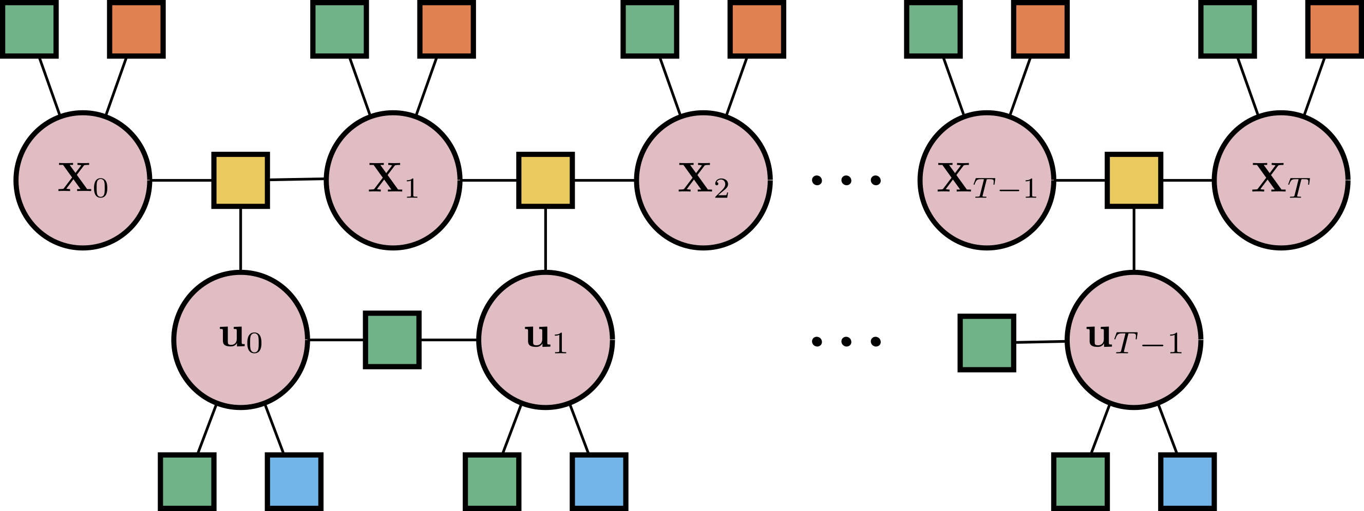
Figure 6: Factor graph modeling the nonlinear MPC control problem.

Figure 7: Our pseudo-omnidirectional platform with four steering and driving wheels.

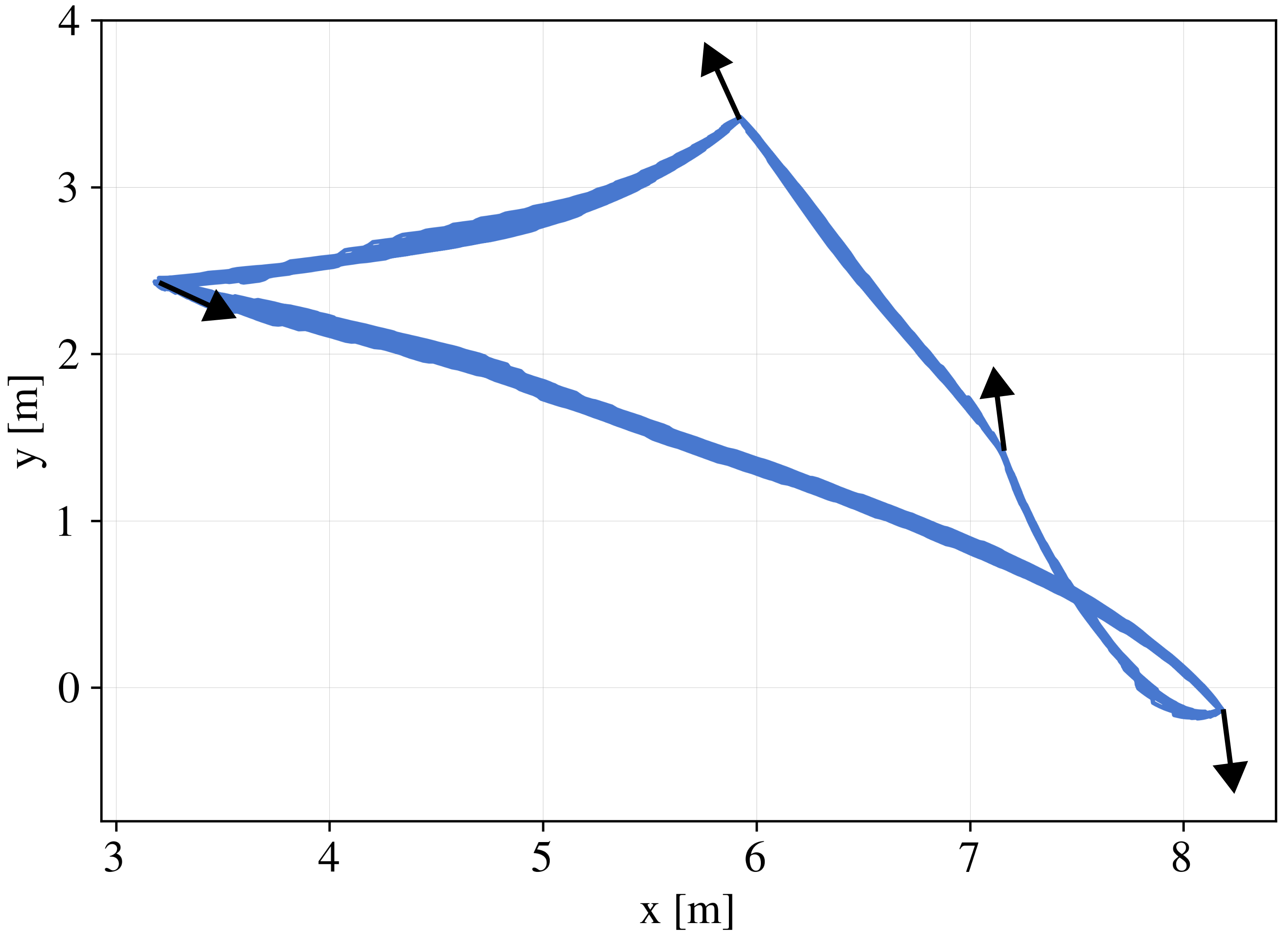
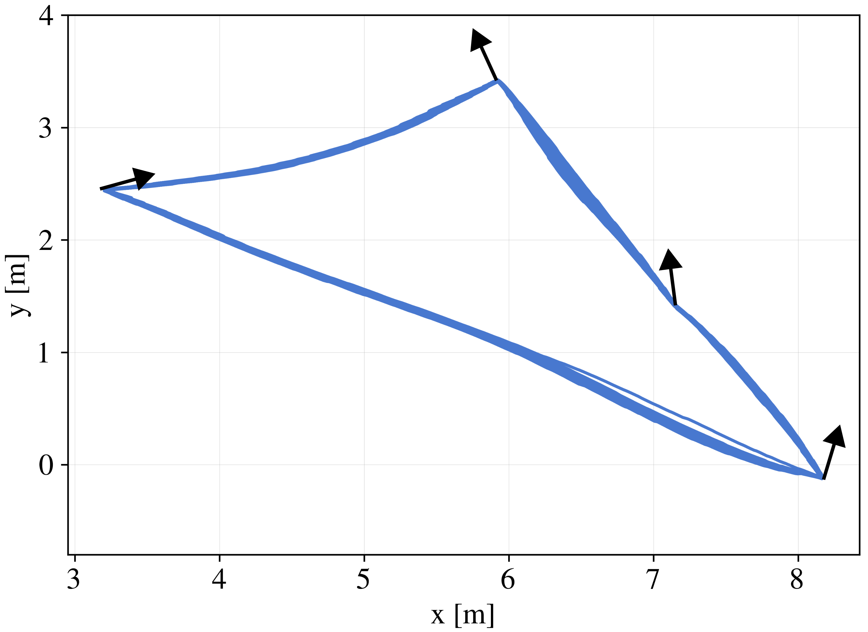
Figure 8: Two sample set of goals, grouped in closed paths. The desired orientation of the goal is represented by the arrows.

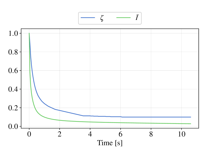
Figure 9: Evolution of damping $\zeta$ and of average number of iterations $\bar{I}$ on one round from goal 5 to goal 6. $\bar{I}$ is divided by its maximum value (1000).

IV-C Factor Graph-