Occupancy Grid Map to Pose Graph-based Map: Robust BIM-based 2D-LiDAR Localization for Lifelong Indoor Navigation in Changing and Dynamic Environments

Abstract

Several studies rely on the de facto standard AMCL method to localize a robot in an OGM extracted from a BIM model. However, most of these studies assume that the BIM model precisely represents the real world, which is rarely true. Discrepancies between the reference BIM model and the real world (Scan-BIM deviations) are not only due to the presence of furniture or clutter but also due to the usual as-planned and as-built deviations that exist with any model created in the design phase. These Scan-BIM deviations may affect the accuracy of AMCL drastically. This paper proposes an open-source method to generate appropriate Pose Graph-based maps from BIM models for robust 2D-LiDAR localization in changing and dynamic environments. First, 2D OGMs are automatically generated from complex BIM models. These OGMs only represent structural elements allowing indoor autonomous robot navigation. Then, an efficient technique converts these 2D OGMs into Pose Graph-based maps enabling a more accurate robot pose tracking. Finally, we leverage the different map representations for accurate, robust localization with a combination of state-of-the-art algorithms. Moreover, we provide a quantitative comparison of various state-of-the-art localization algorithms in three simulated scenarios with varying levels of Scan-BIM deviations and dynamic agents. More precisely, we compare two PF algorithms: AMCL and GMCL; and two GBL methods: Google’s Cartographer and SLAM Toolbox, solving the global localization and pose tracking problems. We found that in a real office environment (under medium level of Scan-BIM deviations) the translational RMSE of AMCL increases by a factor of four (from $8.5\text{\,}\mathrm{cm}$ in the empty environment to $33.7\text{\,}\mathrm{cm}$ in the real one). On the contrary, pose Graph-based algorithms demonstrate their superiority in contrast to particle filter (PF) algorithms, achieving an RMSE of $7.2\text{\,}\mathrm{cm}$, even in the real environment. The numerous experiments demonstrate that the proposed method contributes to a robust localization with an as-designed BIM model or a sparse OGM in changing and dynamic environments, outperforming the conventional AMCL in accuracy and robustness.

1 INTRODUCTION

An accurate localization system is crucial for successful autonomous mobile robot deployment in indoor GPS-denied environments.

The indoor localization problem has been approached by applying several techniques. While some of them rely on the known position of landmarks, such as AprilTags or textual cues, others depend on sensors that have to be installed strategically on the building, such as Beacons or WiFi access points. However, in most cases, the exact location of specific landmarks is not known in advance. On top of that, having additional sensors increases the cost of the navigation stack.

A BIM model, which is available for most of the current architecture, can be used as a reference map for LiDAR localization. Moreover, the additional semantic information of the model can be exploited to create advanced automated robotic tasks, like object inspection [Kim and Peavy (2022)] or painting [Kim et al. (2021)], which at the same time depend on an accurate localization system.

The main issue of using a BIM model or a floor-plan as a reference map for 2D-LiDAR localization is the presence of Scan-BIM deviations. These deviations can be caused by furniture or clutter not present in the model, as-planned and as-built deviations, and dynamic or “quasi-static” changes in the environment. In an effort to address this challenge, we contribute with a system that creates OGMs from BIM models and allows their automatic transformation in pose graph-based maps. These maps are leveraged for quick, memory efficient, and accurate localization in indoor GPS-denied environments, enabling safer autonomous navigation.

More specifically, the following are our contributions:

• A method to extract OGMs out of complex multi-story BIM models to allow path planning and autonomous navigation of robots in indoor GPS-denied environments.

• An efficient open-source method to convert these 2D OGMs into pose graph-based maps for accurate 2D-LiDAR localization and navigation.

• An extensive quantitative comparison of various state-of-the-art 2D LiDAR localization algorithms in three carefully designed simulated scenarios with different levels of Scan-BIM deviations and with and without dynamic agents.

The remainder of this paper is organized as follows. Section 2 introduces the problem formulation of LiDAR localization as well as the main principles behind the particle filter-based and the graph-based localization strategies. Section 3 describes previous work done on BIM-based LiDAR localization. Section 4 introduces our method to generate OGMs from BIM models and pose graph-based maps from OGMs, as well as the proposed employment of these maps for robust localization. Section 5 presents the experimental settings, followed by the results and analysis in section 6. Finally, section 7 concludes our work.

2 THEORETICAL BACKGROUND

Before presenting current state-of-the-art methods, a brief introduction to the theoretical basis behind the two main types of localization algorithms used in this research is provided.

2.1 Localization problem

In this paper, we address the robot pose tracking and global localization problems, i.e., with and without approximated initial pose respectively, given a 3D BIM model as a prior map which omits considerable information about the real environment and assuming that the robot employs a 2D-LiDAR sensor.

In the 2D problem, the pose of the robot at time $t$ is defined as position and orientation $\boldsymbol{x}_{t}=[x,y,\theta]^{\top}$ in the coordinate system of the map.

We aim to estimate the most likely robot’s pose $\boldsymbol{x}_{t}^{*}$ given the measurements $\boldsymbol{z}_{t}$ and the map $\boldsymbol{m}$. Formally, the goal is to compute:

$$\boldsymbol{x}_{t}^{*}=\underset{\boldsymbol{x}}{\arg\max}p\left(\boldsymbol{x}_{t}\mid\boldsymbol{z}_{t},\boldsymbol{m}\right)$$ (1)

Two widely used methods that aim to calculate this estimate are the PF and the GBL algorithms.

2.2 Particle Filter algorithms

PF algorithms, also called MCL methods, are probabilistic approaches that represent the pose estimate with a set of normalized weighted particles. Each particle $\boldsymbol{s}_{t}^{i}=\left\langle\boldsymbol{x}_{t}^{i},\omega_{t}^{i}\right\rangle$ consist of a pose $\boldsymbol{x}_{t}^{i}$ and a weight $\omega_{t}^{i}$.

Initially, a set $\mathcal{M}$ of particles is sampled from a Gaussian distribution around the possible locations of the robot. Subsequently, three steps are repeated iteratively in the algorithm: motion update, importance weighting, and particle resampling. For a more detailed explanation of every step, the reader is referred to ?). In our comparison we implemented AMCL [Pfaff et al. (2006)] and GMCL [Alshikh Khalil and Hatem (2021)] to be tested under different levels of Scan-BIM deviations.

2.3 Graph-based algorithms

Graph-based, also called optimization-based localization methods use previously acquired pose-graph data for pose estimation. This pose-graph contains landmarks of the environment (which can be represented as submaps) associated with nodes (which are the poses from where the landmarks were observed). Additionally, the nodes are bound to each other with spatial constraints. In a sliding window manner, the method not only considers the most recent measurement but a set of them to compute the current pose.

Under the assumption that the measurements are normally distributed and i.i.d., it is possible to represent eq. 1 as a weighted least squares problem. This problem is commonly solved iteratively using the Levenberg-Marquart algorithm.

In this paper we compare Cartographer [Hess et al. (2016)] and SLAM Toolbox [Macenski and Jambrecic (2021)] as GBL algorithms.

While particle filter algorithms are easier to implement and can represent non-Gaussian distributions, graph-based localization algorithms, besides being deterministic, can handle delayed measurements and maintain a recent history of poses. A more exhaustive qualitative comparison is given by ?).

3 RELATED RESEARCH

A BIM model with 3D geometric information can be used as a prior map to accurately localize robots in indoor GPS-denied environments and allow autonomous navigation.This section will overview state-of-the-art methods, which used prior building information, i.e., BIM models or floor plans, to find the correct robot position and orientation.

?) show that the transformation matrix between the reference system of the robot and the map extracted from the BIM model can be retrieved by applying the standard AMCL algorithm.

The same algorithm was used by ?), ?), ?), and ?) to localize a wheeled robot in an OGM generated from the BIM model.

The main difference between these methods relies on how they create the OGM from the BIM model.

While [Follini et al. (2020)] took the vertices of elements that intersect a horizontal plane and used the Open CASCADE viewer to generate an OGM in pgm format with the corresponding resolution and map origin information, [Prieto et al. (2020)] uses the geometry of the spaces in the IFC file and the location and size of each one of the openings.

?) developed a BIRS, enabling the generation and semantic transfer of topological and metric maps from a BIM model to ROS. The tool was further developed in [Karimi et al. (2021)] with an optimal path planner, integrating critical components for construction assessment.

?) implemented a method to convert an IFC file into a ROS-compliant SDF world file suitable for robot task planning. They evaluated their approach for the purpose of indoor wall painting.

Later, to incorporate dynamic objects and for the aim of door inspection, ?) proposed a technique to convert an IFC model into a URDF building world. Once they have the URDF model, they use the PgmMap creator [Yang (2018)] to create an OGM out of it.

?) proposed an approach that instead of using an OGM uses a robot-specific world model representation extracted from an IFC file for 2D-LiDAR localization.

In their factor graph-based localization approach, the system queries semantic objects in its surroundings and creates data associations between them and the laser measurements.

While they demonstrated that the method can track the pose of the robot, it was not evaluated quantitatively.

Instead of using a BIM model, ?) use a CAD-based architectural floor plan for 2D LiDAR-based localization. In their localization system, they implement GICP for scan matching together with a pose graph SLAM system.

Later, they proposed an improved pipeline for long-term localization in dynamic environments ?).

?) uses an OGM obtained from a sliced TLS point cloud a together with human-readable localized cues to assist localization. With their text detection-based localization technique, they can detect known room numbers and thus can robustly handle symmetric environments with structural changes.

While several approaches have emerged aiming to create OGMs from BIM models, none of them deal with complex non-convex models with multiple stories and slanted floors. Moreover, most of the proposed techniques are based on the strong assumption that the BIM model represents the actual current state of the building very precisely, ignoring the presence of possible Scan-BIM deviations due to clutter, furniture, as-planned vs. as-built differences, changes due to long-term operation, or the presence of dynamic agents.

4 METHODOLOGY

Our method can be divided in three main steps: Step 1: Creation of an OGM from an IFC file employing IfcConvert and OpenCV. Step 2: Automatic generation of a Pose Graph-based map out of an OGM with a combination of image processing, coverage path planner, and ray casting. Step 3: Robust localization using particle filter algorithm and graph-based localization system.

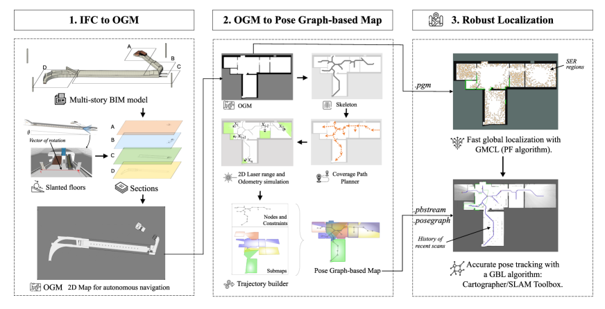
Figure 1: Proposed IFC to Pose Graph-based map for robust 2D-LiDAR localization. In the first step, an OGM is created from Multi-story non-convex BIM models which can have slanted floors, this map is suitable for path planning and autonomous robot navigation. In the second step, a Pose Graph-based map is generated from the OGM. Finally, in the third step, these maps allow fast global localization and robust pose tracking in changing and dynamic environments.

4.1 OGM generation from an IFC

For the creation of suitable 2D OGM for robot localization and navigation from a complex multi-story IFC models the IfcConvert tool of IfcOpenSchell [Krijnen (2015)] and image processing techniques are used.

IfcConvert allows the creation of a 2D map in SVG format with the desired elements in the IFC model that cross a plane at the desired height.

In our case, non-permanent entities such as spaces, windows, and doors are excluded from the resulting 2D OGM by ignoring the corresponding entity names. This exclusion is essential to filter only structural information about the building, enabling further autonomous navigation between the rooms that want to be explored. Besides having the permanent structures in the OGM, and with the aim of global localization and posterior correct pose graph map generation, it is crucial to differentiate between outdoor (unknown) and indoor (navigable) spaces in the OGM. This distinction can be automated creating a second OGM with all the entities in the IFC file (i.e., with doors, windows, and spaces).

The final separation of outdoor (gray color), indoor (white) and obstacle (black) is done based on the contours in the SVG image. OpenCV allows the processing of the contours depending on their hierarchy, i.e., depending if they are inside (child contours) or outside another contour (parent contours).

The resulted file is finally converted to .pgm, which together with its properties (the resolution and origin) in a .yaml file can then be loaded in the robotic system as prior environment information, allowing robot localization, path planning, and autonomous navigation.

A similar procedure can be followed for multi-story level buildings. In the particular case of non-overlapping stories, the different OGMs can be merged in a single one if the relative position between them is known. To maintain this spacial relationship, while obtaining the OGMs, reference auxiliary elements with a height equal to the maximum building’s height can be included in its surroundings. With these additional elements, all the OGMs will have the same dimensions allowing its merging.

Creating 2D OGMs with IfcConvert is relatively straightforward when the desired section is horizontal (parallel with the XY plane). However, if the model has a ramp or a slightly slanted floor, the model must be rotated before the occupancy map is generated.

Favorably, IfcConvert also allows the rotation of the model at the desired angle given a quaternion calculated from the vector of rotation.

4.2 OGM2PGBM: OGM to Pose Graph-based map conversion

The automatic generation of data suitable for GBL methods from BIM models implies the simulation of sequential laser data in the entire navigable space in the model with the corresponding odometry data.

For this aim, the previously generated 2D OGM are used.

Applying the skeleton method proposed by ?) enables the interconnection of all the rooms in a smooth trajectory.

Subsequently, a Wavefront Coverage Path Planner ?) is applied over the navigable area inside a dilated version of the skeleton, allowing finding the waypoints over which the laser will be simulated.

Then, using a ray casting algorithm and without a real-time simulation engine (such as Gazebo), laser sensor data and odometry are simulated following the waypoints found in the previous step. Finally, a trajectory builder merges these sensor data creating an accurate pose graph-based map, serialized as a .pbstream file for Cartographer or as a .posegraph file for SLAM Toolbox. Graph optimization is not required since every scan’s position is known accurately from the simulation.

This pipeline allows the automatic efficient generation of pose graph-based maps (with submaps, nodes, and constraints) from a 2D OGM. As our OGM2PGBM workflow does not require Gazebo for data simulation, it is faster and more portable than a Gazebo-based pipeline, allowing its execution on an isolated manner. Moreover, since the technique does not consider the complete 3D model but only a 2D OGM, it is very efficient. In addition, it can be used from any given OGM, which besides of been generated from a BIM model (with the method presented in the previous section), can be generated out of a floor plan or a previously scanned map.

4.3 Robust Localization

Once the different needed map representations (OGM and pose graph-based maps) are generated from a BIM model, they can be used for robust localization in changing environments. We propose to take advantage of the Self-Adaptive PF of GMCL to spread particles only in the SER regions and solve the global localization problem efficiently. As it is shown later (in Section 6), PF algorithms being able of representing non-Gaussian distributions can solve the global localization faster than graph-based algorithms. Once an estimated pose is found with a covariance smaller than 0.05, the nodes of GMCL are stopped, and a GBL algorithm can be started. For example, to track the pose of the robot accurately, Cartographer can be activated with the start_traj service at the time when GMCL converges and using the .pbstream map generated with the method proposed in Section 4.3. Similarly, SLAM Toolbox can be started with an initial pose, however with a prior .posegraph map.

5 EXPERIMENTS

This section presents the evaluation scenarios designed to evaluate the various techniques and details of the implementation and evaluation.

5.1 Evaluation Scenarios

As illustrated in Figure 2, three different scenarios were conceived to evaluate the different methods. Each scenario increases the level of clutter present in the environment and, therefore, decreases the level of overlap that a perception sensor would have with permanent building objects (such as walls, columns, floors, and ceilings). The latter are the elements that are usually present in a BIM model.

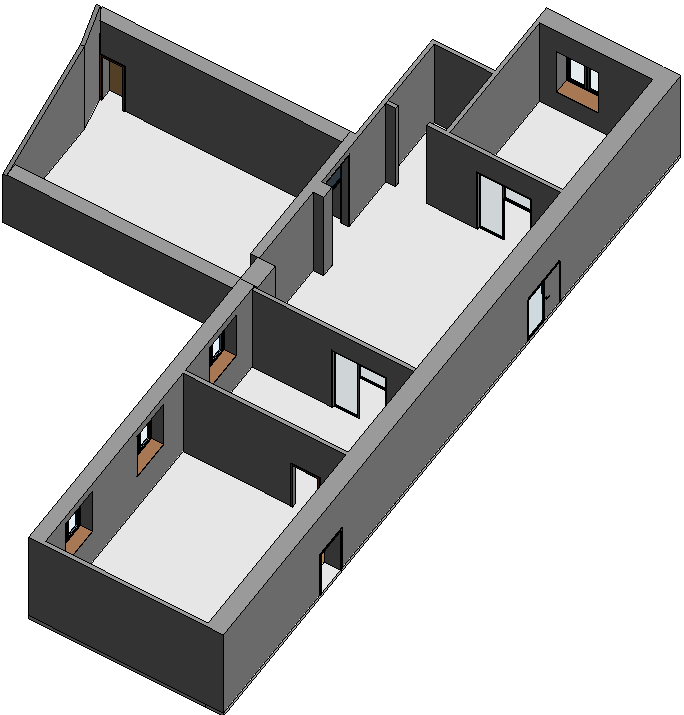
(a) 1

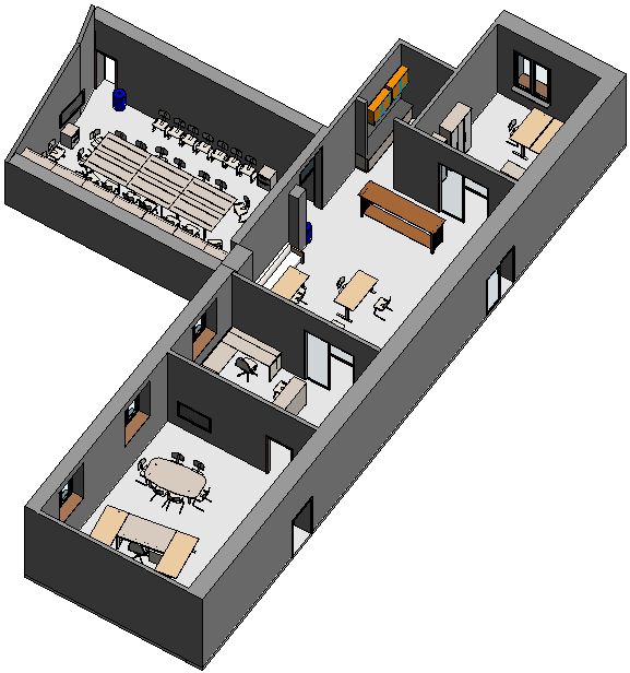
(b) 2

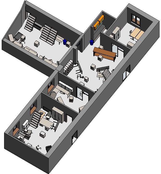
(c) 3

Figure 2: Evaluation Scenarios. (a) Empty Room: represents a typical BIM Model, without furniture; (b) Reality: represents a standard office environment and is based on real-world TLS data; (c) Disaster: is an environment after a simulated disaster with large Scan-BIM deviations.

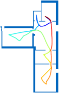
(a)

(b)

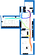
(c)

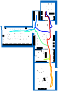
(d)

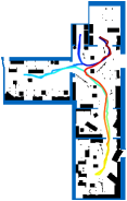
(e)

(f)

Figure 3: Sequences of data with the respective OGMs. (a) and (b) correspond to an empty environment (i.e., without furniture) with and without dynamic agents resp.; (c) and (d) similar but in an scenario with furniture as it is in the real world; (e) and (f) in the disaster environment. To better visualize the different levels of Scan-BIM deviations, the OGM of the empty environment is presented over the other OGMs in blue color. The change in color of the trajectory represents the initial and end position of the robot, with dark blue being the start and red the endpoint.

Additionally, to increase the simulation’s realism level, we added animated walking human models (also called dynamic agents) moving in the environment. In scenarios 1 and 2, five humans walk from each room to the closest exit of that room. In the scenario Nr. 3 (“Disaster”), a total of six people move faster, trying to escape through the main door. Once the agents reach their goal, they start again, moving from their initial planned position in an infinite loop.

5.2 Gazebo Simulation

To simulate the experimental data, we use Gazebo. Once the IFC model is converted to Collada format using IfcConvert, it can be imported in Gazebo. While importing complex IFC models in Gazebo is essential to ensure that every element has its own geometric representation. One way to avoid instantiating multiple objects from the same data is using the export capabilities of Blender.

For trustworthy data simulation, we separate between collision and visual models. Since LiDAR sensors cannot perceive glass materials, windows and glass doors were removed in the collision models.

5.3 Robot Simulation

The robot used for the simulated experiments was the holonomic Robotnik SUMMIT XL equipped with a 2D LiDAR Hokuyo UST-10LX. It was commanded with stable linear and angular velocity of at approximately 1 m/s and 1 deg/s, respectively.

Using the URDF model of this robot it is possible to leverage the different packages of the ROS Navigation Stack for RViz. One of these packages is NAVFN which assumes a circular robot and allows to plan a path from a start point to an endpoint in a grid based on a Costmap.

A Costmap is an inflated version of the given 2D OGM with a specified amplification radius created to avoid the robot colliding with obstacles while navigating through the environment.

To speed up the usage of the OGM for robot simulation, the Gazebo Plug-in PgmMap creator [Yang (2018)], was also implemented, allowing the creation of maps with known origin position. In practice, this step is not required since the alignment between the real world and the map can be retrieved as a localization system result.

It is worth mentioning that using navigational goals instead of single movement commands is very convenient for data simulation since it significantly reduces the probability of collisions, which can make the entire sequence useless.

Following this approach, 2D LiDAR, IMU, Wheel odometry, and ground truth odometry were simulated in the six scenarios (three models with and without dynamic agents). The resulted trajectories of the simulation are presented in Figure 3.

5.4 Implementation details

Due to the stochastic nature of PF algorithms (AMCL and GMCL) and similarly as done by [Alshikh Khalil and Hatem (2021)], these methods were executed 30 times in each sequence, and the average values were calculated.

Similarly as [Zimmerman et al. (2022)], we consider that a method converges when its pose estimate is within a distance of $0.5\text{\,}\mathrm{m}$ from the ground truth pose. If after the first $95\text{\,}\mathrm{\char 37\relax}$ of the sequence, convergence does not happen, then it is considered a failure.

Unfortunately, SLAM Toolbox could not be evaluated for global localization since it does not provide this service. The lifelong mapping mode of SLAM Toolbox was also tested for the matter of completeness; however, it yields to unwanted results, with a poor performance.

6 RESULTS AND ANALYSIS

Table 1: Summary of the quantitative evaluation results for each sequence. Translational RMSE in centimeters and angular RMSE in degrees respectively.

Method	1-1		1-2		2-1		2-2		3-1		3-2
AMCL	8.49	0.44	8.47	0.50	33.68	2.71	37.44	3.26	63.04	3.29	65.12	3.37
GMCL	8.27	0.24	7.86	0.24	24.27	2.57	52.38	4.37	66.60	3.70	126.91	4.46
SLAM Toolbox	3.69	0.17	3.95	0.17	28.69	1.50	23.57	1.50	37.84	1.34	37.96	1.70
Cartographer	4.01	0.24	3.96	0.25	7.19	0.15	4.11	0.21	-	-	-	-

The libraries provided by ?) and ?) were used to calculate the error metrics of the various methods on the different sequences.

6.1 Pose tracking

In Table 1 we present the translational and rotational RMSE for each sequence for each method evaluated on the pose tracking problem with the ground truth from the simulation.

Figure 4 presents a summary of the statistics of the translational errors for all the methods in all sequences.

Overall it can be seen that GBL methods always perform better than PF algorithms in the pose tracking problem.

Among the tested PF algorithms, GMCL performs most of the time better than AMCL. Only in the scenarios 2-2, 3-1, and 3-2, AMCL achieves lower RMSE. In scenarios 2-2 and 3-2 GMCL has a very high translational RMSE.

This shows that the additional filters of GMCL cause the method to be more sensitive to dynamic environments in changing environments.

Regarding the GBL algorithms, SLAM Toolbox achieves the best performance in scenarios 1 and 3. As expected, scenario 3 (with the most significant Scan-BIM deviations) was the most challenging scenario for all the methods. On top of that, in this scenario, the pure localization mode of Cartographer always found wrong data associations, resulting in wrong relative constraints that cause localization failure. Therefore Cartographer could not be quantitatively evaluated in this environment, even when an initial approximated pose was provided. Nonetheless, Cartographer achieved an impressive performance in the scenario 2 (real-world scenario), accomplishing a translational RMSE four times lower than SLAM Toolbox, in the environment without dynamic agents ($7.19\text{\,}\mathrm{cm}$ and $28.69\text{\,}\mathrm{cm}$ respectively) and almost six times lower in the scenario with dynamic agents ($4.11\text{\,}\mathrm{cm}$ and $23.57\text{\,}\mathrm{cm}$ respectively).

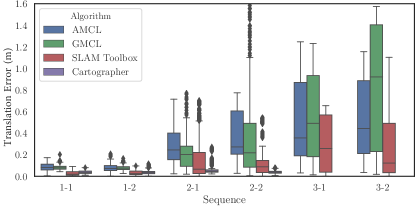
Figure 4: Statistics of the pose error estimates in translation for each method on the six evaluation scenarios.

6.2 Global localization

Figure 5: Convergence time in seconds for the various methods in the different scenarios.

The performance of the different methods regarding convergence time is presented in Figure 5.

GMCL, thanks to its Self-Adaptive PF, performs the best in the global localization problem. Only in scenario 1-2 Cartographer shows a slight superiority. Meanwhile, AMCL takes always at least twice as long compared to the other methods to converge to a good pose. In addition, it does not converge in scenario 2-1.

Due to the high level of Scan-BIM deviations, none of the implemented methods converges while trying to solve the global localization problem in scenario 3.

7 CONCLUSIONS

In this paper, besides contributing with methods to create OGMs from BIM models and transforming them to pose graph-based maps for robust localization, we provide an extensive comparison of diverse state-of-the-art localization 2D-LiDAR algorithms in three different levels of Scan-BIM deviations, with and without dynamic agents.

We found that GBL algorithms overperform PF algorithms in the pose tracking problem. In the case of a map with very low (or negligible) Scan-BIM deviations, SLAM Toolbox achieves the best performance. On the contrary, if the map has a medium level of Scan-BIM deviations (for example, due to large pieces of furniture or as-planned and as-built differences), as in a real-world office building, Cartographer is the best performing method. However, in a case where the level of changes in the environment is too high (such as in scenario 3), SLAM Toolbox, while with a relatively high error, would be the best option among the tested localization algorithms.

The fact that PF algorithms only consider the most recent observation to update the belief of the current pose gives them certain robustness to deal with high ambiguity scenarios (such as scenario 3). However, it also causes high inaccuracies when the level of Scan-BIM deviations is medium (such as in scenario 2). On the other hand, GBL algorithms taking advantage of a recent history of observations, can handle better this real-world scenario and can track the robot’s pose more accurately.

Nonetheless, GMCL perform better for the global localization problem than GBL algorithms.

In general we recommend using a GBL algorithm for accurate BIM-based (or floor plan-based) 2D LiDAR pose tracking in real-world environments and GMCL for global localization.

To facilitate the correct implementation of GBL algorithms, we contribute with an open-source method to create efficiently accurate pose graph-based maps from any OGM.

In addition, we provide with a method to create OGMs from complex multi-story BIM models, which additionally can be leveraged for path planning and autonomous navigation.

State-of-the-art SLAM techniques have switched from using particle filters to graph-based optimization approaches, based on our experiments, we can conclude that it will be analogously advantageous for most localization systems.

8 FUTURE WORK

In the light of the experimental results and motivated by related research, we believe that the following are promising future research directions:

Consider not only 2D-LiDAR information but also 3D-LiDAR sensor data is a promising direction to reliably handle large levels Scan-BIM deviations, as partially shown by ?) and ?).

Fuse multiple sensor modalities, such as IMU, RGB-D cameras, together with LiDAR sensors, would increase the robustness of a localization method to deal with fast angular movements and deprecated scenarios, as demonstrated by ?) and ?).

To achieve major robustness, the extraction of detailed information from a BIM model, such as the position of room numbers labels, doors and windows can support to solve the global localization problem even in symmetric environments, as done by ?) and ?).

9 ACKNOWLEGEMENTS

The presented research was conducted in the frame of the project “Intelligent Toolkit for Reconnaissance and assessmEnt in Perilous Incidents” (INTREPID) funded by the EU’s research and innovation funding programme Horizon 2020 under Grant agreement ID: 883345.

References

- Alshikh Khalil and Hatem (2021) Alshikh Khalil, M. A. & I. Hatem (2021). Gmcl as a proposed replacement to amcl in ros for mobile robots localization in known-based 2d environments.
- Blum et al. (2021) Blum, H., F. Milano, R. Zurbrügg, R. Siegward, C. Cadena, & A. Gawel (2021). Self-improving semantic perception for indoor localisation.
- Boniardi et al. (2017) Boniardi, F., T. Caselitz, R. Kummerle, & W. Burgard (2017). Robust lidar-based localization in architectural floor plans. In 2017 IEEE/RSJ International Conference on Intelligent Robots and Systems (IROS), pp. 3318–3324. IEEE.
- Boniardi et al. (2019) Boniardi, F., T. Caselitz, R. Kümmerle, & W. Burgard (2019). A pose graph-based localization system for long-term navigation in cad floor plans. Robotics and Autonomous Systems 112, 84–97.
- Follini et al. (2020) Follini, C., V. Magnago, K. Freitag, M. Terzer, C. Marcher, M. Riedl, A. Giusti, & D. T. Matt (2020). Bim-integrated collaborative robotics for application in building construction and maintenance. Robotics 10(1), 2.
- Grupp (2017) Grupp, M. (2017). evo: Python package for the evaluation of odometry and slam.
- Haque et al. (2020) Haque, A., A. Elsaharti, T. Elderini, M. A. Elsaharty, & J. Neubert (2020). Uav autonomous localization using macro-features matching with a cad model. Sensors (Basel, Switzerland) 20(3).
- Hendrikx et al. (2021) Hendrikx, R. W. M., P. Pauwels, E. Torta, H. J. Bruyninckx, & M. J. G. van de Molengraft (2021). Connecting semantic building information models and robotics: An application to 2d lidar-based localization. In 2021 IEEE International Conference on Robotics and Automation (ICRA), pp. 11654–11660. IEEE.
- Hess et al. (2016) Hess, W., D. Kohler, H. Rapp, & D. Andor (2016). Real-time loop closure in 2d lidar slam. In 2016 IEEE International Conference on Robotics and Automation (ICRA), pp. 1271–1278. IEEE.
- Karimi et al. (2021) Karimi, S., R. G. Braga, I. Iordanova, & D. St-Onge (2021). Semantic navigation using building information on construction sites.
- Karimi et al. (2020) Karimi, S., I. Iordanova, & D. St-Onge (2020). An ontology-based approach to data exchanges for robot navigation on construction sites.
- Kim and Peavy (2022) Kim, K. & M. Peavy (2022). Bim-based semantic building world modeling for robot task planning and execution in built environments. Automation in Construction 138, 104247.
- Kim et al. (2021) Kim, S., M. Peavy, P.-C. Huang, & K. Kim (2021). Development of bim-integrated construction robot task planning and simulation system. Automation in Construction 127, 103720.
- Krijnen (2015) Krijnen, T. (2015). Ifcopenshell.
- Lee et al. (1994) Lee, T.-C., R. L. Kashyap, & C.-N. Chu (1994). Building skeleton models via 3-d medial surface axis thinning algorithms. CVGIP: Graphical Models and Image Processing 56(6), 462–478.
- Lin and Zhang (2021) Lin, J. & F. Zhang (2021). R3live: A robust, real-time, rgb-colored, lidar-inertial-visual tightly-coupled state estimation and mapping package.
- Macenski and Jambrecic (2021) Macenski, S. & I. Jambrecic (2021). Slam toolbox: Slam for the dynamic world. Journal of Open Source Software 6(61), 2783.
- Moura et al. (2021) Moura, M. S., C. Rizzo, & D. Serrano (2021). BIM-based Localization and Mapping for Mobile Robots in Construction. 2021 IEEE International Conference on Autonomous Robot Systems and Competitions, ICARSC 2021, 12–18.
- Pfaff et al. (2006) Pfaff, P., W. Burgard, & D. Fox (2006). Robust monte-carlo localization using adaptive likelihood models. In H. I. Christensen (Ed.), European Robotics Symposium 2006, Volume 22 of Springer Tracts in Advanced Robotics, pp. 181–194. Berlin/Heidelberg: Springer-Verlag.
- Prieto et al. (2020) Prieto, S. A., B. Garcia de Soto, & A. Adan (2020). A methodology to monitor construction progress using autonomous robots. In H. Osumi (Ed.), Proceedings of the 37th International Symposium on Automation and Robotics in Construction (ISARC), Proceedings of the International Symposium on Automation and Robotics in Construction (IAARC). International Association for Automation and Robotics in Construction (IAARC).
- Thrun et al. (2005) Thrun, S., W. Burgard, & D. Fox (2005). Probabilistic robotics. Intelligent robotics and autonomous agents. Cambridge Mass.: MIT Press.
- Wilbers et al. (2019) Wilbers, D., C. Merfels, & C. Stachniss (2019). A comparison of particle filter and graph-based optimization for localization with landmarks in automated vehicles. In 2019 Third IEEE International Conference on Robotic Computing (IRC), pp. 220–225. IEEE.
- Xu et al. (2022) Xu, W., Y. Cai, D. He, J. Lin, & F. Zhang (2022). Fast-lio2: Fast direct lidar-inertial odometry. IEEE Transactions on Robotics, 1–21.
- Yang (2018) Yang, H. (2018). Github - pgmmapcreator: Create pgm map from gazebo world file for ros localization.
- Zelinsky et al. (1993) Zelinsky, A., R. A. Jarvis, J. C. Byrne, & S. Yuta (Eds.) (1993). Planning paths of complete coverage of an unstructured environment by a mobile robot, Volume 13 of Proceedings of international conference on advanced robotics. Citeseer.
- Zhang and Scaramuzza (2018) Zhang, Z. & D. Scaramuzza (2018). A tutorial on quantitative trajectory evaluation for visual (-inertial) odometry. In 2018 IEEE/RSJ International Conference on Intelligent Robots and Systems (IROS), pp. 7244–7251.
- Zimmerman et al. (2022) Zimmerman, N., L. Wiesmann, T. Guadagnino, T. Läbe, J. Behley, & C. Stachniss (2022). Robust onboard localization in changing environments exploiting text spotting.