Effect of long-range hopping on dynamic quantum phase transitions of an exactly solvable free-fermion model: non-analyticities at almost all times

Abstract

In this work, we investigate quenches in a free-fermion chain with long-range hopping which decay with the distance with an exponent $\nu$ and has range $D$. By exploring the exact solution of the model, we found that the dynamic free energy is non-analytical, in the thermodynamic limit, whenever the sudden quench crosses the equilibrium quantum critical point. We were able to determine the non-analyticities of dynamic free energy $f(t)$ at some critical times $t^{c}$ by solving nonlinear equations. We also show that the Yang-Lee-Fisher (YLF) zeros cross the real-time axis at those critical times. We found that the number of nontrivial critical times, $N_{s},$ depends on $\nu$ and $D$. In particular, we show that for small $\nu$ and large $D$ the dynamic free energy presents non-analyticities in any time interval $\Delta t\sim 1/D\ll 1$, i.e., there are non-analyticities at almost all times. For the spacial case $\nu=0$, we obtain the critical times in terms of a simple expression of the model parameters and also show that $f(t)$ is non-analytical even for finite system under anti-periodic boundary condition, when we consider some special values of quench parameters. We also show that, generically, the first derivative of the dynamic free energy is discontinuous at the critical time instant when the YLF zeros are non-degenerate. On the other hand, when they become degenerate, all derivatives of $f(t)$ exist at the associated critical instant.

I Introduction

Equilibrium phase transitions (PTs) have been detail studied and observed in several compounds in the last two centuries (S. Sachdev, 2011; H. E. Stanley, 1987; Sondhi et al., 1997). Along the lines (or planes, or points) that separate the distinct phases, the thermodynamic functions are non-analytic. Due to this fact, the systems present unusual physical properties close to these lines. In general, we can not understand the phenomena close to the transition lines by a simple picture, such as the Fermi liquid for instance. For this reason, this subject has been of great interest for several physicist communities. The non-analyticity of the thermodynamic functions is encoded in the zeros of the partition function ${\cal Z}$, the so-called Yang-Lee-Fisher (YLF) zeros (Yang and Lee, 1952; Lee and Yang, 1952; M. E. Fisher, 1965). In general, the zeros of ${\cal Z}(q)=\text{Tr}\left(e^{-qH}\right)$ happen for $q=\beta+i\alpha$, where $\beta=\frac{1}{k_{B}T}$ and $\alpha\neq 0$. In the thermodynamic limit, however, these zeros can touch the real temperature axis yielding to non-analyticities of the Helmholtz free energy $F=-k_{B}T\ln\left({\cal Z}(\beta)\right)$. For a recent experimental verification of this phenomenon, see, for instance, Refs. Wei and Liu, 2012; Peng et al., 2015. A similar equilibrium partition function that is also studied is the boundary partition function $\mathcal{Z}^{b}(\beta)=\left\langle\psi^{b}\left|e^{-\beta H}\right|\psi^{b}\right\rangle$, i.e., the partition function ruled by the Hamiltonian $H$ with boundaries described by the boundary state $\left|\psi^{b}\right\rangle$ separated by $\beta$ (J. L. Cardy, 1989; J. L. Cardy and D. C. Lewellen, 1991; LeClair et al., 1995).

In the last years (Heyl et al., 2013; Andraschko and Sirker, 2014; Vajna and Dóra, 2014; Karrasch and Schuricht, 2013; Canovi et al., 2014; Vajna and Dóra, 2015; Halimeh and Zauner-Stauber, 2017; Žunkovič et al., 2018; Fläschner et al., 2018; Jafari et al., 2019; Jafari, 2019; Guo et al., 2019; Zauner-Stauber and Halimeh, 2017; Jurcevic et al., 2017; Homrighausen et al., 2017; Hoyos et al., 2022a), the concept of YLF zeros has been applied to sudden quenches: a parameter $\delta$ of a system Hamiltonian $H\left(\delta\right)$ changes from $\delta_{0}\rightarrow\delta$ at the time instant $t=0$. Specifically, the dynamical analog of the boundary partition function is the return probability $Z(t)=\left\langle\psi_{0}\left|e^{-iH(\delta)t}\right|\psi_{0}\right\rangle$, where $\left|\psi_{0}\right\rangle$ is the ground state of the Hamiltonian $H\left(\delta_{0}\right)$. The dynamical analog of the free energy is $f(t)=-\frac{1}{N}\ln\left(\left|Z(t)\right|^{2}\right)$, where $N$ is the number of degrees of freedom, and can also be a non-analytic function at some critical time $t^{c}$. For a review and generalizations to other out-of-equilibrium scenarios see, e.g., Ref. Heyl, 2018.

The quantum quench protocol we consider here is the following: the system is prepared in the ground state of $H(\delta_{0})$ and then is time-evolved according to $H(\delta)$, being $\delta$ some tuning parameter of $H$. The non-analytical behavior of $f$ in time was called dynamical quantum phase transition (DQPT) (Heyl et al., 2013) and was recently observed in experiments (Jurcevic et al., 2017; Guo et al., 2019; Fläschner et al., 2018). It is important to mention that, by now, it is well established that there is no one-to-one correspondence between DQPTs and equilibrium phase transitions (Andraschko and Sirker, 2014; Vajna and Dóra, 2014; Canovi et al., 2014; Vajna and Dóra, 2015; Halimeh and Zauner-Stauber, 2017; Žunkovič et al., 2018; Jafari, 2019).

Experimental observation of the DQPTs was observed recentely  (Jurcevic et al., 2017), where trapped ions were used to simulate the transverse-field Ising chain with long range interaction. The long range interaction between two spins $i$ and $j$ is given by $J_{i,j}=\Omega^{2}\nu_{R}\sum_{m}\frac{b_{im}b_{jm}}{\mu^{2}-\nu_{m}^{2}}$ (Islam et al., 2013) and depends on the experimental setup, namely: the Rabi frequency $\Omega$ of the laser, the ion mass of the single ion via the recoil frequency $\nu_{R}$ associated with the dipole force, the orthonormal mode component of the ith ion $b_{im}$ with mode $m$ and frequency $\nu_{m}$, as well as the symmetric detuning $\mu$ of the beatnote from the spin-flip transition  (Porras and Cirac, 2004; Islam et al., 2013; Jurcevic et al., 2017; Monroe et al., 2021; Marino et al., 2022). It has been observed in trapped ion experiments that the long range coupling $J_{i,j}$ can be approximated as $J_{i,j}\sim 1/|i-j|^{\alpha}$ where $0<\alpha<3$ depends on the laser detuning $\mu$ (Islam et al., 2013; Jurcevic et al., 2017; Zhang et al., 2017; Joshi et al., 2022).

The effect of the long-range interactions in the context of the DQPTs were investigated in the transversal-Field Ising chain (Jurcevic et al., 2017; Homrighausen et al., 2017; Halimeh and Zauner-Stauber, 2017; Zauner-Stauber and Halimeh, 2017; Žunkovič et al., 2018). All those studies were done numerically since the long-range interaction, in general, breaks integrability (exceptions exist and can be found in, e.g., Zunkovic et al., 2016; Kosior and Sacha, 2018). Although numerical results can give strong evidence of the DQPTs, those methods are limited. In particular, the studies based on exact diagonalization and/or matrix product state (MPS) are limited by the size of the system, and/or by the bond dimension, as well as limited to short times. In principle and strictly according to the YLF zeros theory, the DQPTs manifest only in the thermodynamic limit. In this sense, a rigorous proof of the existence of a DQPT in the transversal-Field Ising chain with long-range interaction is still missing. In this vein, it is highly desirable to have a deep understanding of the long-range interaction effects in the context of DQPTs through analytical results. Insights into this issue may be gained by considering the free fermions with long-range hopping, since the model can be mapped, by using the Jordan-Wigner transformation, in a XX chain with long range interaction. Although in this case, multiple spin interactions appear (M. Suzuki, 1971; Eloy and Xavier, 2012; Jones, 2022). Very recently, the effect of the long range hopping in the context of the DQPT were investigated in few models, like some variant of the Kitaev chain (Dutta and Dutta, 2017; Defenu et al., 2019; Uhrich et al., 2020) (see also Refs. Zunkovic et al., 2016; Kosior and Sacha, 2018). Motivated by the aforementioned facts, we investigate DQPTs in an exactly solvable free fermion model with long-range hoppings.

The paper is organized as follows: In Sec. II, we present the model and its exact diagonalization. Analytical expressions for the dynamic free energy and the YLF zeros are determined in Sec. III together with numerical results. Our concluding remarks are given in Sec. IV.

II The model

We consider a free fermion chain with long-range hoppings under twisted boundary condition given by the Hamiltonian

$$H(\delta)=\sum_{j=1}^{L}\frac{1+\left(-1\right)^{j}\delta}{2}\sum_{\ell=1}^{D}J_{j,2\ell-1}\left(c_{j}^{\dagger}c_{j+2\ell-1}^{\phantom{\dagger}}+{\rm H.c.}\right).$$ (1)

We consider systems of $L$ sites in which $L$ is even. The hopping amplitude decays as $J_{j,\ell}=J2^{\nu}(\ell+1)^{-\nu}$. Here, the constant $J$ sets the energy (or inverse time) unit of the system (and, from now on, is set to $J=1$), and $c_{j+L}=\exp\left(-\phi\pi i\right)c_{j}$ ($1\leq j\leq L$), where $\phi$ defines the type of boundary condition: $\phi=0$ means periodic boundary condition (PBC) and $\phi=1$ means anti-periodic boundary condition (APBC). The exponent $\nu\geq 0$ controls the decay of the hopping amplitude with the distance, $D$ is the hopping range, and $\delta$ is the dimerization parameter which tunes the system across an equilibrium quantum phase transition (QPT) at $\delta=0$. For $D=1$, this model recovers the dimerized chain with nearest-neighbor hopping, also known as Su-Schrieffer-Heeger (SSH) chain (Su et al., 1979). This model, for some particular choice of the parameters, was used to study symmetry-resolved entanglement entropy (Ares et al., 2022; Jones, 2022). This is an interesting model because it allows one to investigate the effects of long-range hopping and is amenable to be solved by free-fermion techniques.

Note that the gauge transformation $c_{j}\rightarrow e^{-i\pi\Phi j/L}c_{j}$ makes the Hamiltonian translational invariant and, thus, can be diagonalized by the Fourier series. For the sake of completeness, we present the main steps below. First, we introduce the new fermionic operators $\gamma_{q}$ and $\eta_{q}$ by

$$c_{2j}=\sqrt{\frac{2}{L}}\sum_{q}e^{2iqj}\eta_{q},\mbox{ and }c_{2j-1}=\sqrt{\frac{2}{L}}\sum_{q}e^{iq\left(2j-1\right)}\gamma_{q},$$ (2)

where the momenta are $\mbox{ }q=q_{n}=\frac{2\pi}{aL}\left(n-\frac{\phi}{2}\right)$, $n=1,2,\dots,L/2$, and, from now on, we set the lattice spacing to $a=1$. In terms of $\gamma_{q}$ and $\eta_{q}$ the Hamiltonian is

$$H = \sum_{q}\left(\begin{array}[]{cc}\gamma_{q}^{\dagger}&\eta_{q}^{\dagger}\end{array}\right)\left(\begin{array}[]{cc}0&C_{q}-i\delta S_{q}\\ C_{q}+i\delta S_{q}&0\end{array}\right)\left(\begin{array}[]{c}\gamma_{q}^{\phantom{\dagger}}\\ \eta_{q}^{\phantom{\dagger}}\end{array}\right),$$ (8)

$$= \sum_{q}\omega_{q,\delta}\left(\alpha_{+,q,\delta}^{\dagger}\alpha_{+,q,\delta}^{\phantom{\dagger}}-\alpha_{-,q,\delta}^{\dagger}\alpha_{-,q,\delta}^{\phantom{\dagger}}\right),$$ (9)

where

$$C_{q}=C_{q}(\nu,D) = \sum_{\ell=1}^{D}\ell^{-\nu}\cos\left((2\ell-1)q\right),$$ (10)

$$S_{q}=S_{q}(\nu,D) = \sum_{\ell=1}^{D}\ell^{-\nu}\sin\left((2\ell-1)q\right),$$ (11)

$$\omega_{q,\delta}=\omega_{q,\delta}(\nu,D) = \sqrt{C_{q}^{2}+\delta^{2}S_{q}^{2}},$$ (12)

and

$$\alpha_{\pm,q,\delta}=\frac{1}{\sqrt{2}}\left(e^{i\theta_{q,\delta}}\gamma_{q}\pm e^{-i\theta_{q,\delta}}\eta_{q}\right)$$ (13)

are the eigen-operators associated to positive and negative branches of the dispersion relation $\pm\omega_{q,\delta}(\nu,D)$. Here, $\cos 2\theta_{q,\delta}=C_{q}/\omega_{q,\delta}$ and $\sin 2\theta_{q,\delta}=\delta S_{q}/\omega_{q,\delta}$.

Finally, notice that

$$C_{\frac{\pi}{2}-q}=-C_{\frac{\pi}{2}+q},\mbox{ and }S_{\frac{\pi}{2}-q}=S_{\frac{\pi}{2}+q},$$ (14)

and that the ground state of $H(\delta)$ is

$$\left|\psi_{0}(\delta)\right\rangle=\prod_{q}\alpha_{-,q,\delta}^{\dagger}\left|0\right\rangle,$$ (15)

where the product is over all $q$’s in Eq. (2).

It is worth mentioning that for some special values of $\nu$ and $D$, the functions $C_{q}$ and $S_{q}$ can also be written in terms of some well known functions, as depicted in Table 1. For $\nu=\infty$ or $D=1$, Eq. (12) recovers that of the nearest-neighbor hopping problem $\omega_{q,\delta}=\sqrt{\cos^{2}(q)+\delta^{2}\sin^{2}(q)}$. The case $\nu=0$ and $D=L/4$ is very peculiar and presents some anomalous characteristics (see Appendix A): (i) The ground-state energy $E_{0}\sim aL\ln L+bL$ is not extensive. (ii) Different boundary conditions lead to distinct behaviors. For PBC (APBC), the system is gapless (gapped) at half filling. In addition, the difference $E_{0}^{\text{APBC}}-E_{0}^{\text{PBC}}\sim-L\ln L$.

Table 1: The functions $C_{q}(\nu,D)$ and $S_{q}(\nu,D)$ for some special values of $\nu$ and $D$. $\text{Li}_{\nu}(z)$ is the polylogarithm function of order $\nu$.

		$C_{q}(\nu,D)$		$S_{q}(\nu,D)$
$\nu=0$		$\frac{\sin\left(2Dq\right)}{2\sin q}$		$\frac{1-\cos\left(2Dq\right)}{2\sin(q)}$
$\nu=1$ $D=\infty$		$-1/2\left[\cos\left(q\right)\ln\left(\left|2\sin q/2\right|\right)-\sin\left(q\right)(\pi-2q)\right]$		$1/2\left[\cos\left(q\right)(\pi-2q)+\sin\left(q\right)\ln\left(\left|2\sin q/2\right|\right)\right]$
$\nu=2$ $D=\infty$		$\frac{\pi^{2}}{6}-\frac{2q}{2}+\frac{q^{2}}{4}$		$-\int_{0}^{q}\ln\left(2\sin(t/2)\right)dt$
$\nu=\infty$		$\cos\left(q\right)$		$\sin\left(q\right)$
$D=\infty$		$\text{Re}\left(e^{-iq}\text{Li}_{\nu}\left(e^{i2q}\right)\right)$		$\text{Im}\left(e^{-iq}\text{Li}_{\nu}\left(e^{i2q}\right)\right)$

III Results

III.1 The dynamic free energy and the YLF zeros

As we already mentioned, in our quench protocol the system is initialized in $\left|\psi_{0}(\delta_{0})\right\rangle$, the ground state of $H(\delta_{0})$, and time-evolved according to $H(\delta)$. Only $\delta$ is changed in the sudden quench, $\nu$ and $D$ remain constants. The return probability amplitude $Z(t)=\left\langle\psi_{0}(\delta_{0})\left|e^{-iH(\delta)t}\right|\psi_{0}(\delta_{0})\right\rangle$ can be evaluated following the same procedure of Ref. (Hoyos et al., 2022a, b). For completeness, we present below the main steps.

To time-evolve $\left|\psi_{0}(\delta_{0})\right\rangle$, we need the relation between the pre- and post-quench eigen-operators $\alpha_{\pm,q,\delta_{0}}$ and $\alpha_{\pm,q,\delta}$ [see Eq. (9)]. This task is simple, since the wavenumbers $q$ in (2), and, therefore, $\gamma_{q}$ and $\eta_{q}$, do not depend on $\delta$. Then, from Eq. (13), we find that

$$\alpha_{-,q,\delta_{0}}^{\dagger}=\cos\left(\Delta\theta_{q,\delta,\delta_{0}}\right)\alpha_{-,q,\delta}^{\dagger}+i\sin\left(\Delta\theta_{q,\delta,\delta_{0}}\right)\alpha_{+,q,\delta}^{\dagger},$$ (16)

where $\Delta\theta_{q,\delta,\delta_{0}}=\theta_{q,\delta}-\theta_{q,\delta_{0}}$. Therefore,

$$Z(t) = \left\langle 0\left|\prod_{q}\alpha_{-,q,\delta_{0}}e^{-iHt}\prod_{k}\alpha_{-,k,\delta_{0}}^{\dagger}\right|0\right\rangle$$ (17)

$$= \prod_{q}\left[\cos\left(\omega_{q,\delta}t\right)+ig_{q,\delta,\delta_{0}}\sin\left(\omega_{q,\delta}t\right)\right],$$

where $0\leq g_{q,\delta,\delta_{0}}=\frac{C_{q}^{2}+\delta\delta_{0}S_{q}^{2}}{\omega_{q,\delta}\omega_{q,\delta_{0}}}\leq 1$.

Finally, the dynamic free energy $f(t)\equiv-L^{-1}\ln\left|Z(t)\right|^{2}$ is

$$f(t)=-\frac{1}{L}\sum_{q}\ln\left[\cos^{2}\left(\omega_{q,\delta}t\right)+g_{q,\delta,\delta_{0}}^{2}\sin^{2}\left(\omega_{q,\delta}t\right)\right],$$ (18)

and, in the thermodynamic limit, we can replace the sum by the integral

$$f(t)=-\intop_{0}^{\pi/2}\frac{dq}{\pi}\ln\left[\cos^{2}\left(\omega_{q,\delta}t\right)+g_{q,\delta,\delta_{0}}^{2}\sin^{2}\left(\omega_{q,\delta}t\right)\right],$$ (19)

where the properties (14) where used to shorten the integration limit.

Let $\zeta_{n,m}=t_{n,m}+i\tau_{n}$ (or $\zeta_{q_{n},m}=t_{q_{n},m}+i\tau_{q_{n}}$) be the YLF zeros of $Z$. From Eq. (17), it is simple to show that

$$\zeta_{q_{n},m}=\frac{\left(m-\frac{1}{2}\right)\pi+\frac{i}{2}\ln\left(\frac{1+g_{q_{n},\delta,\delta_{0}}}{1-g_{q_{n},\delta,\delta_{0}}}\right)}{\omega_{q_{n},\delta}},$$ (20)

were $m\in\mathbb{N}_{+}$ is the $m$th accumulation line of YLF zeros, and $n=1,\dots,\frac{L}{2}$ labels the $n$th wavenumber $q_{n}$ in (2). Although there are $\frac{L}{2}$ YLF zeros per accumulation line, not all of them are distinct because of (14). For $\frac{L}{2}$ odd, there are $\frac{1}{2}\left(\frac{L}{2}-1\right)$ distinct zeros (which are doubly degenerated), and one (for $q=\pi$ for PBC and $q=\frac{\pi}{2}$ for APBC) has $\left|\tau_{q_{n}}\right|=\infty$. Thus, effectively there are $\frac{1}{2}\left(\frac{L}{2}-1\right)$ zeros. For PBC and $\frac{L}{2}$ even, there are $\frac{1}{2}\left(\frac{L}{2}-2\right)$ distinct zeros (which are doubly degenerated), and 2 zeros (for $q=\frac{\pi}{2}$ and $\pi$) with $\left|\tau_{q_{n}}\right|=\infty$. For APBC and $\frac{L}{2}$ even, there are $\frac{L}{4}$ doubly degenerated distinct zeros.

The DQPTs occur whenever $\tau_{q_{n}}=0$ and, thus, from Eq. (20), they can only happen if $C_{q^{c}}^{2}+\delta\delta_{0}S_{q^{c}}^{2}=0$, i.e.,

$$T_{q^{c}}^{2}(\nu,D)\equiv\frac{S_{q^{c}}^{2}(\nu,D)}{C_{q^{c}}^{2}(\nu,D)}=-\frac{1}{\delta\delta_{0}}.$$ (21)

Notice the necessary condition $\delta\delta_{0}<0$ which corresponds to the quench crossing the equilibrium QPT of the model at $\delta_{\text{eq}}^{c}=0$. Once the set $\left\{q^{c}\right\}$ is determined from Eq. (21), the time instants of the DQPTs are simply $t_{\left\{q^{c}\right\},m}^{c}=\frac{\left(2m-1\right)\pi}{2\omega_{q^{c},\delta}}$. Due to the properties (14), if $q^{c}$ is a solution of (21), so is $\pi-q^{c}$. In addition, they provide the same YLF zero since $\omega_{q,\delta}=\omega_{\pi-q,\delta}$. Thus, it is sufficient to consider only the values of $q$ in the domain $\left[0,\frac{\pi}{2}\right]$ when solving for $\left\{q^{c}\right\}$ in (21).

In general, Eq. (21) admits no solution for finite systems since $\left\{q_{n}\right\}$ in Eq. (2) is a discrete set. Nonetheless, as reported in Appendix A, for some special values of $\nu$, $D$, $\delta$ and $\delta_{0}$, Eq. (21) admits solutions for finite systems and, thus, for a real-time instant $t^{c}$, $f(t^{c})$ is non-analytic even for finite $L$. Non-analyticities in finite-size systems were also reported in Refs. Andraschko and Sirker, 2014; Karrasch and Schuricht, 2013.

III.2 The case of nearest-neighbor ($D=1$) and third-nearest-neighbor ($D=2$) hoppings

For completeness, we now briefly review the results for $D=1$ and compare them with the case $D=2$. It turns out that this comparison is very instructive to understand the case of generic $D$.

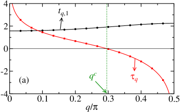
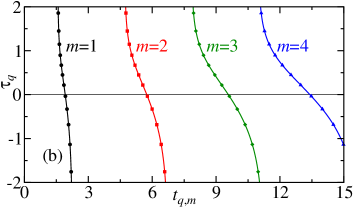
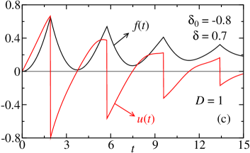
Figure 1: In (a) and (b) we show the Yang-Lee-Fisher zeros $\zeta_{q_{n},m}$ [Eq. (20)] for $D=1$. (a) $t_{q,1}$ and $\tau_{q}$ as a function of the momentum $q$ (for accumulation line $m=1$). (b) The complex-time plane (for $m=1,\dots,4$). (c) The associated dynamical free energy $f$ [Eq. (19)] and its time derivative $u$ as a function of $t$. In (a), $q^{c}$ denotes the momentum associated with the real-time YLF zero. The symbols in (a) and (b) correspond to the allowed values of $q$ for a finite chain of length $L=60$. The continuous lines in (a), (b) and (c) correspond to the thermodynamic limit. The sudden quench is from $\delta_{0}=-0.8$ to $\delta=0.7$.

For $D=1$ and $\delta\delta_{0}<0$, Eq. (21) gives a single solution $q^{c}=\arctan\left(\frac{1}{\sqrt{-\delta\delta_{0}}}\right)\in\left[0,\frac{\pi}{2}\right]$ [see Fig. 1(a)]. This means that each accumulation line in (20) provides only one real-time instant $t_{q^{c},m}=\left(m-\frac{1}{2}\right)\pi\sqrt{\frac{1-\delta\delta_{0}}{\delta\left(\delta-\delta_{0}\right)}}$ in which the dynamic free energy is non-analytic in the thermodynamic limit [see Fig. 1(b)]. This non-analyticity is manifest as a cusp in $f\left(t\right)$ (or a discontinuity in the dynamic internal energy $u\equiv\frac{\partial f}{\partial t}$) at $t=\zeta_{q^{c},m}=t_{q^{c},m}$ [see Fig. 1(c)]. Note that for the case $D=1$, the results do not depend on the value of $\nu$.

Precisely, the non-analyticity of the dynamic free energy can be quantified by analyzing the behavior of the YLF zeros near the real-time axis. From the Weierstrass factorization theorem (Yang and Lee, 1952; Lee and Yang, 1952; M. E. Fisher, 1965), the singular part of the free energy due to the zero in the $m$th accumulation line is $f_{\text{n-a}}=-L^{-1}\sum_{n}\ln\left(\zeta-\zeta_{q_{n},m}\right)+\text{c.c.}$ . Here, c.c. stands for complex conjugate and accounts for the zeros of $\bar{Z}$ (the complex conjugate of $Z$). In the thermodynamic limit, $\zeta_{q_{n},m}$ in Eq. (20) can be expanded near $q^{c}$ [see Fig. 1(a)]. Then, the real-time non-analyticity of the dynamic internal energy is quantified by

$$u_{\text{n-a}}=-\frac{1}{\pi}\int_{-\delta q}^{\delta q}\frac{d\tilde{q}}{\Delta t-\left(A_{q^{c},m}-iB_{q^{c}}\right)\tilde{q}}+\text{c.c.},$$ (22)

where $\Delta t=t-\zeta_{q^{c},m}=t-t_{q^{c},m}$, $\tilde{q}=q-q^{c}$, $A_{q^{c},m}=\left.\frac{\partial t_{q,m}}{\partial q}\right|_{q=q^{c}}=-\frac{\delta_{0}\left(1-\delta^{2}\right)}{\left(\delta-\delta_{0}\right)\sqrt{-\delta\delta_{0}}}t_{q^{c},m}$, $B_{q^{c}}=-\left.\frac{\partial\tau_{q}}{\partial q}\right|_{q=q^{c}}=2\left|\delta\right|\omega_{q^{c},\delta}^{-3}$, and $\delta q$ is a positive constant whose value is unimportant for quantifying the non-analyticity of $u$. The numerical prefactor is $\pi^{-1}$ and not $\left(2\pi\right)^{-1}$ because we are using the properties (14) to take into account the other YLF zero in the interval $q\in\left[\frac{\pi}{2},\pi\right]$. By a simple integration (via residues, for instance), we can show that first derivative of the dynamic free energy has a discontinuity given by

$$\Delta u\left(\zeta=\zeta_{q,m}\right)=\lim_{\Delta t\rightarrow 0^{+}}u_{\text{n-a}}-\lim_{\Delta t\rightarrow 0^{-}}u_{\text{n-a}}=-\frac{4B_{q^{c}}}{A_{q^{c},m}^{2}+B_{q^{c}}^{2}}.$$ (23)

This is because the pole at $\tilde{q}=\frac{\Delta t}{A_{q^{c},m}-iB_{q^{c}}}$ crosses the real-$\tilde{q}$ axis when $\Delta t$ changes sign. We have confirmed this result via numerical integration of (19).

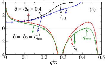
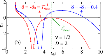
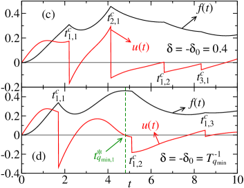
Figure 2: In (a) and (b) we show the Yang-Lee-Fisher zeros $\zeta_{q_{n},m}$ [Eq. (20)] for $D=2$ and $\nu=1/2$. (a) $t_{q,1}$ and $\tau_{q}$ as a function of the momentum $q$ (for accumulation line $m=1$) and (b) in the complex-time plane (for $m=1$). (c) and (d) The associated dynamical free energy $f$ [Eq. (19)] and its time derivative $u$ as a function of $t$. We consider two sudden quenches: (c) from $\delta_{0}=-0.4$ to $\delta=0.4$ (fulfilling $-\frac{1}{\delta\delta_{0}}>T_{q_{\text{min}}}^{2}$) and (d) from $\delta_{0}=-T_{q_{\text{min}}}^{-1}\left(\nu,D\right)$ to $\delta=T_{q_{\text{min}}}^{-1}\left(\nu,D\right)\approx 0.52$ (see legends). In (a), $q_{\text{min}}$ denotes the momentum associated with the real-time YLF zero which only touches the real-time axis. In (b) and (d), the corresponding time instant $t_{q_{\text{min}}}$ is highlighted. The symbols in (a) and (b) correspond to the allowed values of $q$ for a finite chain of length $L=60$. The continuous lines in (a), (b), (c) and (d) correspond to the thermodynamic limit.

For $D=2$ and $\delta\delta_{0}<0$, the situation is more involved. If $v<\log_{2}3\approx 1.585$, Eq. (21) admits two additional solutions if $-\frac{1}{\delta\delta_{0}}>T_{q_{\text{min}}}^{2}(\nu,D)=\left(\frac{3+2^{\nu}}{3-2^{\nu}}\right)^{3}\left(\frac{2^{\nu}+1}{2^{\nu}-1}\right)$ [see Fig. 2(a)]. This is because $T_{q}^{2}(\nu,D)$ has a local minimum at $q_{\text{min}}=\frac{1}{2}\arccos\left(-\frac{4^{\nu}+3}{2^{2+\nu}}\right)$. Thus, each accumulation line of YLF zeros crosses the real-time axis at three different instants [see Fig. 2(b)]. The corresponding density of YLF zeros crossing the real-time axis is a constant. Hence, as in the case $D=1$, the corresponding non-analyticities are cusps in $f(t)$ at those time instants [see Figs. 2(c) and (d)].

However, it is not straightforward to anticipate the resulting singularity when the two additional YLF zeros become degenerate, i.e., when $-\frac{1}{\delta\delta_{0}}=T_{q_{\text{min}}}^{2}(\nu,D)$. Following the same steps as in Eq. (22), the singular part of the dynamical internal energy around the time instant $\zeta_{q_{\text{min}},m}=t_{q_{\text{min}},m}^{*}$ is

$$u_{\text{n-a}}=-\frac{1}{\pi}\int_{-\delta q}^{\delta q}\frac{d\tilde{q}}{\Delta t-\left(A_{q_{\text{min}},m}\tilde{q}-\frac{i}{2}C_{q_{\text{min}}}\tilde{q}^{2}\right)}+\text{c.c.}$$ (24)

where $\Delta t=t-\zeta_{q_{\text{min}},m}=t-t_{q_{\text{min}},m}^{*}$, $\tilde{q}=q-q_{\text{min}}$, $A_{q_{\text{min}},m}=\left.\frac{\partial t_{q,m}}{\partial q}\right|_{q=q_{\text{min}}}$, $C_{q_{\text{min}}}=-\left.\frac{\partial^{2}\tau_{q}}{\partial q^{2}}\right|_{q=q_{\text{min}}}$, and $\delta q$, as before, is an unimportant positive constant. As for the case $D=1$, the non-analytical behavior of $u_{\text{n-a}}$ comes when a pole crosses the real-$\tilde{q}$ axis. However, we now face the situation where the integrand of $u_{\text{n-a}}$ has two poles. It is easy to see that one of the poles always remains far from the real-$\tilde{q}$ axis and, thus, does not contribute to the non-analyticity. The other one does not cross the real-$\tilde{q}$ axis either. It only touches it when $\Delta t=0$. As a result, the limit $u_{\text{n-a}}(t)$ as $t\rightarrow t_{q_{\text{min}}}$ exists, i.e., $\Delta u=\lim_{\Delta t\rightarrow 0^{+}}u_{\text{n-a}}-\lim_{\Delta t\rightarrow 0^{-}}u_{\text{n-a}}=0$. The same reasoning applies to all derivatives of $u$. Finally, we conclude that although $f$ is non-analytic at $t_{q_{\text{min}}}$, it is a smooth function (all derivatives exist) at that time instant [see Fig. 2(d)]. Nonetheless, we recall that this non-analyticity poses a numerical challenge in computing $f$ and its derivatives at that time instant.

In analogy to the Ehrenfest’s classification of the order of the equilibrium phase transitions (Jaeger, 1998), we could classify the order of the DQPTs by the lowest derivative of the dynamic free energy that is discontinuous at the transition. With this classification in mind, we observe that when the YLF zeros are not degenerate, the DQPT is of first order. On the other hand, when the YLF zeros become degenerate, the DQPT is of infinite order. It is then tempting to state that this is the dynamic analog of the Berezinskii-Kosterlitz–Thouless (BKT) transition of equilibrium systems. However, BKT transition has a continuous of YLF zeros in one of the phases. Here, there is no continuous distribution of YLF zeros after or before the instant of non-analyticity $t_{q_{\text{min}},m}^{*}$.

III.3 Numerical results

As we show below, this feature of two dynamical QPTs becoming degenerate (either by fine-tuning $\delta\delta_{0}$ or $\nu$) and the associated cusps annihilating each other is a general feature for all other values of the hopping range $D$.

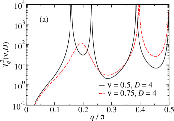
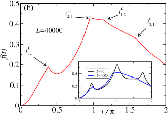
Figure 3: (a) $T_{\nu,D}^{2}$ vs. $q$ for $D=4$ and $\nu=0.5$ and $0.75$. (b) The dynamic free energy $f(t)$ vs. $t$ for a system of size $L=40\,000$, $D=4$, $\nu=0.5$, and $\delta_{0}=-\text{$\delta=0.5$}$ [meaning Eq. (21) has three solutions for $0<q<\frac{\pi}{2}$]. The arrows indicate the cusp positions, which are located at $t_{k,m}^{c}$ (see text). Inset: $f(t)$ for $L=40$ and $L=4000$.

We plot in Fig. 3(a) $T_{q}^{2}(\nu,D)\equiv\frac{S_{q}^{2}(\nu,D)}{C_{q}^{2}(\nu,D)}$ [see Eqs. (10) and (11)] for $\nu=0.5$ and $D=4$. Notice that $T_{\nu,D}^{2}$ diverges for $q$’s such that $C_{q}(\nu,D)=0$. When $\nu$ is sufficiently small, $T_{\nu,D}^{2}$ has $D-1$ local minima in the domain $q\in\left[0,\frac{\pi}{2}\right]$. This means that, for sufficiently large $-\frac{1}{\delta\delta_{0}}$, there are $2D-1$ solutions of Eq. (21). Let $\left\{q_{k}^{c}\right\}$ be the set of solutions of Eq. (21) for generic values $-\frac{1}{\delta\delta_{0}}>0$. Then, $k$ runs from $1$ to $N_{s}$, where $1\leq N_{s}\leq 2D-1$. The corresponding critical times are $t_{k,m}^{c}=\frac{\left(2m-1\right)\pi}{2\omega_{q_{k}^{c},\delta}}$. As a representative example, we plot in Fig. 3(b) $f(t)$ for $\delta_{0}=-\delta=0.5$ and $L=40\,000$. For these parameters, we have that $N_{s}=3$ with $t_{1,1}^{c}\approx 0.380\pi$, $t_{1,2}^{c}\approx 0.954\pi$, $t_{1,3}^{c}\approx 1.591\pi$, and $t_{2,1}^{c}\approx 1.141\pi$. The corresponding non-analyticities are cusps. Evidently, these cusps become rounded for finite systems (see, for instance, the inset of Fig. 3(b)). However, for the case $\nu=0$, non-analyticities occur even for finite systems (see Appendix A).

As previously argued, the number of minima in $T_{q}^{2}$ is $D-1$ for sufficiently small $\nu$, yielding up to $N_{s}=2D-1$ solutions of Eq. (21) (critical time instants per accumulation line). This number has to diminish when $\nu$ increases as $N_{s}=1$ for $\nu\rightarrow\infty$. This is clearly demonstrated in Fig. 3(a) for $\nu=0.75$. Notice that, instead of only local minima, $T_{q}^{2}$ develops local maxima for larger values of $\nu$. This means that the number of critical time instants $N_{s}$ per accumulation line [solutions ] is a non-monotonic function of the quench parameters $\delta$ and $\delta_{0}$. This non-trivial behavior is demonstrated in Figs. 4(a) and (b) where we plot $N_{s}$ as a function of $\nu$ and $\delta$ for fixed $\delta_{0}=1$ and $D=4$ and $40$. Notice that $N_{s}$ always change by $\pm 2$ as these solutions always appear or disappear in pairs. At the transition lines, two solutions degenerate. The resulting non-analiticity is a smooth one as demonstrated for the case $D=2$.

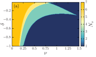
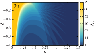
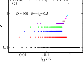
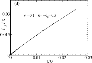
Figure 4: (a) The number of solutions of Eq. (21), $N_{s}$, as a function of $\nu$ and $\delta$ for fixed $\delta_{0}=1$ and (a) $D=4$ and (b) $D=40$. (c) The critical times $t_{k,1}^{c}$ for various values of $\nu$, $D=400$ and $\delta_{0}=-\delta=0.5$. (d) The earliest critical instant $t_{1,1}^{c}$ vs. $1/D$ for $\nu=0.1$ and $\delta_{0}=-\delta=0.5$.

Having discussed the cases of large and small $\nu$, and small $D$, we now discuss the interesting case of small $\nu$ and $D\gg 1$. As we have argued there can be $2D-1$ solutions of Eq. (21). This means the existence of many critical time instants per accumulation line. More interesting, it can be demonstrated that the largest critical time instant is of order unity and the smallest one is of order $D^{-1}$ [see Fig. 4(d)]. As shown in Fig. 4(c), these time instants are somewhat evenly distributed in the interval $\left[\sim D^{-1},\sim 1\right]$ (see more details in Appendix A). Intriguingly, this means that for large values of $D$ the dynamic free energy $f(t)$ will present a large number of non-analyticities in time. This is not only because the number of critical time instants is of order $D$ per accumulation line. As many of those instants happen at $t^{c}\sim D^{-1}$, they “reappear” yet at short time-scales in the other accumulation lines. As a result, $f(t)$ has non-analyticities at almost all times if the quantum quench crosses the transition, $D$ is sufficiently large, and $\nu$ is sufficiently small (see Fig. 5).

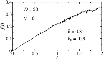
Figure 5: The dynamical free energy $f$ as a function of time $t$ in the case $D=50$ and $\nu=0$ for the quantum quench from $\delta_{0}=-0.9$ to $\delta=0.8$. Many non-analyticities appear already at short time scales.

IV Further discussions and conclusions

We studied the dynamic free energy $f(t)$ of a free fermion chain with long-range hopping couplings, which is described by Eq. (1), focusing on its non-analyticities and the associated Yang-Lee-Fisher zeros.

For effective short-range hoppings (small $D$ or large $\nu$) the YLF zeros cross the real-time axis only in a few instants per accumulation line. In contrast, when the hoppings are sufficiently long ranged (large $D$ and small $\nu$), the number of times the YLF zeros cross the real-time axis increases with $D$ and are more or less evenly spread in the short time interval $0<Jt\lesssim 1$, where $J$ is the microscopic energy scale.

We point out that these many non-analyticities are different from other cases studied in the literature, where the YLF zeros accumulate in an area on the complex-time plane. This is the case for the Kitaev honeycomb model (Schmitt and Kehrein, 2015) and for disordered systems exhibiting dynamical Griffiths singularities (Hoyos et al., 2022a). In the thermodynamic limit, the infinitely many zeros crossing the real-time axis yield to non-analyticities only at the edges of those distributions of zeros. Here, for the model Hamiltonian (1), the zeros do not become continuously distributed over an area on the complex-time plane. They remain distributed in lines that cross the real-time axis in many different time instants. Evidently, when the distance between these singularities increases beyond numerical or experimental resolution, they will appear as a smooth function of time, resembling the case of continuously distributed zeros over a time window.

We emphasize that the singularities are prominent only in sufficiently large systems (rigorously, only in the thermodynamic limit), especially when $D$ is large and $\nu$ small. Therefore, the observation of these many singularities in the current cold-atom platform, where the system size is not too large, may be a challenging task. Perhaps, the best way to circumvent this obstacle is to consider model with anti-periodic boundary condition, $D=L/4$, and $\nu=0$ (see Appendix A). For this situation, the YLF zeros lie on the real-time axis even for finite systems. We note that anti-periodic boundary conditions can be realized by considering the one dimensional chain with periodic boundary condition with a magnetic field passing through the ring. For a particular choice of the flux magnetic, it is possible to map this model to one with the anti-periodic boundary condition (see, for instance, Refs. Byers and Yang, 1961; Kohn, 1964; Poilblanc, 1991).

To the best of our knowledge, long-range interaction effects in the context of DQPTs have only been studied for the transverse-Field Ising chain (Jurcevic et al., 2017; Homrighausen et al., 2017; Halimeh and Zauner-Stauber, 2017; Zauner-Stauber and Halimeh, 2017; Žunkovič et al., 2018). Although the model studied here is different, the present work may shed light on what happens in other models. For instance, in the transverse-field Ising model anomalous cusps (associated with the emergence of new cusps) in the dynamic free energy were reported when $\nu\lesssim 2.2$, at least for some quench parameters (Halimeh and Zauner-Stauber, 2017). These cusps were denominated as anomalous simply because they are not equally spaced in time. As we have explicitly shown, new cusps not evenly separated in time appear for sufficiently long-range hopping (small $\nu$) in a non-trivial fashion (see Fig. 4) as predicted by Eq. (21). It is then desirable to understand Eq. (21) in a more fundamental way and/or generalize it to other systems, in particular, to non-integrable ones. To this end, we recast Eq. (21) is terms of general quantities and find that it is equivalent to $\delta_{0}\omega_{q,\delta}^{2}+\delta\omega_{q,\delta_{0}}^{2}=0$. Thus, in the lack of a better analogy, the number of YLF zeros (or cusps) equals the number of Fermi point pairs of this “weighted dispersion” with zero “chemical potential”. While this is a simple fact for the model we studied, it would be desirable to verify it to other models. For the conventional nearest-neighbor transvere-field Ising chain, the analogous relation can be obtained by recasting the results of Ref. Heyl et al., 2013: it is simply $\omega_{q,g}^{2}+\omega_{q,g_{0}}^{2}=\left(g-g_{0}\right)^{2}$, where the dispersion relation is $\omega_{q,g}=\sqrt{\left(g-\cos q\right)^{2}+\sin^{2}q}$ and $g=h/J$ is the ratio between the transverse field and the ferromagnetic coupling. Again, one needs to find the Fermi points of a weighted dispersion with chemical potential $\left(g-g_{0}\right)^{2}$. We emphasize that, in both models, the YLF zeros are determined uniquely by the knowledge of the dispersion relation and of the pre- and post-quench parameters. It certainly desirable to verify whether this remains true for other models.

Finally, we mention that smaller the value of $\nu$, harder is the detection of the non-analyticities numerically. In particular, the cusps become rounded if the system size is not sufficiently large [see Fig. 3] precluding its detection with exact diagonalization. On the other hand, powerful numerical techniques such as the tDMRG or the MPS use, typically, a time step $\Delta t\sim 0.01/J$ to evolve the initial state. Our results indicate that such time step is not sufficiently small to detect the non-analyticities that appear already at short time scales when $1/(DJ)<0.01/J$ (or $D\gtrsim 100).$

Appendix A The case $\nu=0$

In this appendix, we consider the special case that $\nu=0$, where Eqs. (10) and (11) become

$$C_{q}=\frac{\sin\left(Dq\right)\cos\left(Dq\right)}{\sin q}\mbox{ and }S_{q}=\frac{\sin^{2}\left(Dq\right)}{\sin q}.$$ (25)

A.1 Critical time instants

We need to solve Eq. (21) with the care of having $\omega_{q}\neq 0$. Thus, we need to solve

$$\cos^{2}\left(Dq^{c}\right)+\delta_{0}\delta\sin^{2}\left(Dq^{c}\right)=0.$$ (26)

As we are interested in solutions in the interval $q\in[0,\frac{\pi}{2}]$, then,

$$q_{k}^{c}=\frac{1}{D}\left((k-1)\pi+\arcsin\left(\frac{1}{\sqrt{1-\delta\delta_{0}}}\right)\right),\ k=1,...,\frac{D}{2}.$$ (27)

As we already mentioned, in the Sec. III, to solve Eq. (26) we need that $D\ll L,$ otherwise, there are not enough q’s to satisfy this equation. Once we determine critical values of $q$ that satisfy Eq. (26) we obtain the critical times $t_{i,n}^{c}=\frac{(2n-1)\pi}{2\omega_{q_{i}^{c}}(\delta)}$, $n=1,2,...$, which are given by

$$t_{k,m}^{c}=\left(m-\frac{1}{2}\right)\pi\frac{1-\delta\delta_{0}}{\sqrt{\delta(\delta-\delta_{0})}}\sin\left(q_{k}^{c}\right).$$ (28)

A.1.1 The limit $D\gg 1$

In this limit, the first critical instants ($k\ll D$) of each accumulation line $m$ become

$$t_{k,m}^{c}\approx\left(m-\frac{1}{2}\right)\pi\frac{1-\delta\delta_{0}}{\sqrt{\delta(\delta-\delta_{0})}}\left(\frac{(k-1)\pi+\arcsin\left(\frac{1}{\sqrt{1-\delta\delta_{0}}}\right)}{D}\right).$$ (29)

Thus, they vanish $\sim D^{-1}$.

A.1.2 The case $D=L/4$ and $\delta\delta_{0}=-1$

When $\delta\delta_{0}=-1$, Eq. (27) becomes $q_{k}^{c}=\frac{\pi}{2D}\left(2k-\frac{3}{2}\right)$. The Fourier wavevectors in (2) are $q_{n}=\frac{2\pi}{L}\left(n-\frac{\phi}{2}\right)$. Thus, interestingly, when $D=L/4$ and the anti-periodic boundary condition is considered ($\phi=1$), all critical wavevectors $q_{k}^{c}$ exist even for finite systems (evidently, $L$ is a multiple of $4$). The associated critical instants are

$$t_{k,m}^{c}=\left(2m-1\right)\pi\frac{1}{\sqrt{1+\delta^{2}}}\sin\left(q_{k}^{c}\right).$$ (30)

Notice also that, because the zeros of $Z$ are on the real-time axis even for finite systems, the dynamic free energy diverges at $t_{m,k}^{c}$. Similar non-analyticities at finite systems were observed in other models (Andraschko and Sirker, 2014; Karrasch and Schuricht, 2013; Hoyos et al., 2022b). We illustrate this peculiar behavior of the $f(t)$ in Fig. 6 for a quench where $\delta=-\frac{1}{\delta_{0}}=2$ and $L=16$ and $L=1\,600$. The peaks are finite due to the finite time step we used ($\sim 10^{-4}$). Evidently, $f\left(t\right)$ becomes analytic in the thermodynamic limit as there will be a continuous distribution of YLF zeros over the real-time axis.

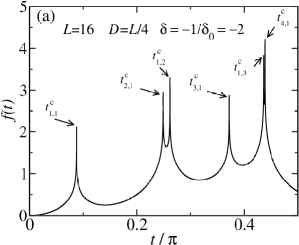
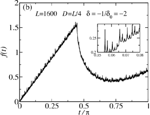
Figure 6: (a) The dynamic free energy $f(t)$ vs. $t/\pi$ for the case $\nu=0$, $D=L/4$, $\delta=-\frac{1}{\delta_{0}}=-2$. (a) For a system size $L=16$. The arrows indicate the critical time positions given by Eq. (30). (b) The same as (a) but $L=1\,600$. Inset: shows a zoom of the region close to $t=0.06\pi$.

A.2 Ground state energy for $D=L/4$

We now compute the ground state energy for systems with PBC ($\phi=0$) and APBC ($\phi=1$), $\nu=0$, and $D=L/4$. The dispersion (12) becomes

$$\omega_{q_{n},\delta}=\frac{\sqrt{\phi+\delta^{2}\left(1+2\left(1-\phi\right)\left(-1\right)^{n}\right)^{2}}}{2\sin q_{n}},$$ (31)

for $n=1,...,\frac{L}{2}$, except for $n=\frac{L}{2}$ and $\phi=0$. Instead, in that case, $\omega_{\pi,\delta}=\frac{L}{4}$. Notice that the system is gapless (gapful) for PBC (APBC) $\phi=0$ ($\phi=1$) regardless of the value of the dimerization parameter $\delta$. A similar situation appears in the topological insulators (TIs). However, in the TIs the bulk is gapped under PBC and there are gapless boundary states for OBC. In the present model, we have gapless states in the bulk for the PBC case, and a gapped state for $\phi\neq 0$. In Fig. 7(a), we illustrate the dispersion relation Eq. (31) for $L=100$ and $\delta=0.5$ for the model with PBC and APBC. It is interesting to note that, in the thermodynamic limit, the system with PBC has two degenerate flat bands.

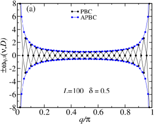
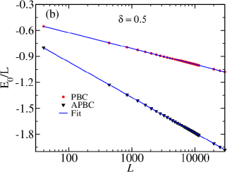
Figure 7: (a) The dispersion relation $\pm\omega_{q,\delta}(\nu,D)$ vs. $q$ for systems under PBC and APBC (see legend) with $L=100$, $\nu=0$, $\delta=0.5$ and $D=L/4$. The symbols are the data obtained from Eqs. (32) and (35). The solid lines connect the fitted points using Eqs. 34 and 36.

The ground state energy $E_{0}^{\text{APBC}}(\delta,\nu=0)$ for the system with APBC is

$$E_{0}^{\text{APBC}}(\delta,0)=-\frac{\sqrt{1+\delta^{2}}}{2}\sum_{n=1}^{\frac{L}{2}}\frac{1}{\sin q_{n}}.$$ (32)

We can replace a sum by a integral by using the Euler-Maclaurin sum

$$\sum_{m=0}^{n}F(a+kh)=\frac{1}{h}\int_{a}^{b}F(q)dq+\frac{1}{2}\left(F(b)+F(a)\right)+R,$$ (33)

where $R$ is the residual term. So,

$$E_{0}^{\text{APBC}}(\delta,0) = -L\frac{\sqrt{1+\delta^{2}}}{4\pi}\Bigl{\{}\int_{\pi/L}^{\pi-\pi/L}\frac{dq}{\sin q}+{\displaystyle\frac{2\pi}{L\sin(\pi/L)}}$$ (34)

$$+\frac{{\displaystyle 2\pi R}}{L}\Bigr{\}},$$

$$= -L\frac{\sqrt{1+\delta^{2}}}{2\pi}\Bigl{\{}\ln\left[\frac{\cos(\pi/2L)}{\sin(\pi/2L)}\right]+{\displaystyle\frac{\pi}{L\sin(\pi/L)}}$$

$$+\pi a_{1}\Bigr{\}},$$

where we use the fact that the residual term $R=La_{1}$. We were not able to obtain the exact value of $a_{1}$. However, we obtain that $a_{1}=0.08596$ by fitting the exact data Eq. (32) with Eq. (34) [see Fig. 7(b)]. We verify that $a_{1}$ does not depend on $\delta$. For large values of $L$, the energy per site becomes $E_{0}^{\text{APBC}}(\delta,0)/L=-\frac{\sqrt{1+\delta^{2}}}{2\pi}\left[\ln\left(2L/\pi\right)+2+\pi a_{1}\right]$. Note that the energy is not extensive. However, we can recover the extensivity if we consider the volume of the system as $V=L\ln L$.

For periodic boundary conditions, the ground state energy for $L$ multiple of $4$ is

$$E_{0}^{\text{PBC}}(\delta,0)=-\frac{L}{4}-\left|\delta\right|\sum_{m=0}^{\frac{L}{4}-1}\frac{1}{\sin\left(2\pi/L(2m+1)\right)}.$$ (35)

Similarly as the APBC case, we obtain

$$E_{0}^{\text{PBC}}(\delta,0) = -\frac{L}{4}-L\frac{\left|\delta\right|}{2\pi}\Bigl{\{}\ln\left[\frac{\cos(\pi/L)}{\sin(\pi/L)}\right]+{\displaystyle\frac{2\pi}{L\sin(2\pi/L)}}$$ (36)

$$+2\pi a_{2}\Bigr{\}},$$

where $a_{2}=0.04297\approx a_{1}/2$ as expected since the residual term depends on the interval and on $h$, which are basically the same in the thermodynamic limit. In this case, for large values of $L$, the energy per site becomes $E_{0}^{\text{PBC}}(\delta,0)/L=-\frac{1}{4}-\frac{\left|\delta\right|}{2\pi}\left[\ln\left(L/\pi\right)+2+2\pi a_{2}\right]$. Note that $E_{0}^{\text{APBC}}-E_{0}^{\text{PBC}}\sim-\left(\sqrt{1+\delta^{2}}-\left|\delta\right|\right)L\ln(L$).

References

- S. Sachdev (2011) S. Sachdev, Quantum Phase Transitions, 2nd ed. (Cambridge University Press, 2011).
- H. E. Stanley (1987) H. E. Stanley, Introduction to Phase Transitions and Critical Phenomena (Oxford University Press, 1987).
- Sondhi et al. (1997) S. L. Sondhi, S. M. Girvin, J. P. Carini, and D. Shahar, “Continuous quantum phase transitions,” Rev. Mod. Phys. 69, 315–333 (1997).
- Yang and Lee (1952) C. N. Yang and T. D. Lee, “Statistical theory of equations of state and phase transitions. i. theory of condensation,” Phys. Rev. 87, 404–409 (1952).
- Lee and Yang (1952) T. D. Lee and C. N. Yang, “Statistical theory of equations of state and phase transitions. ii. lattice gas and ising model,” Phys. Rev. 87, 410–419 (1952).
- M. E. Fisher (1965) M. E. Fisher, The Nature of Critical Points, (Lectures in Theoretical Physic. Vol. viic) ed. (W. E. Brittin, New York: Golden and Breach, 1965).
- Wei and Liu (2012) Bo-Bo Wei and Ren-Bao Liu, “Lee-yang zeros and critical times in decoherence of a probe spin coupled to a bath,” Phys. Rev. Lett. 109, 185701 (2012).
- Peng et al. (2015) Xinhua Peng, Hui Zhou, Bo-Bo Wei, Jiangyu Cui, Jiangfeng Du, and Ren-Bao Liu, “Experimental observation of lee-yang zeros,” Phys. Rev. Lett. 114, 010601 (2015).
- J. L. Cardy (1989) J. L. Cardy, “Boundary conditions, fusion rules and the Verlinde formula,” Nucl. Phys. B 324, 581 (1989).
- J. L. Cardy and D. C. Lewellen (1991) J. L. Cardy and D. C. Lewellen, “Bulk and boundary operators in conformal field theory,” Phys. Lett. B 259, 274 (1991).
- LeClair et al. (1995) A. LeClair, G. Mussardo, H. Saleur, and S. Skorik, “Boundary energy and boundary states in integrable quantum field theories,” Nuclear Physics B 453, 581–618 (1995).
- Heyl et al. (2013) M. Heyl, A. Polkovnikov, and S. Kehrein, “Dynamical quantum phase transitions in the transverse-field ising model,” Phys. Rev. Lett. 110, 135704 (2013).
- Andraschko and Sirker (2014) F. Andraschko and J. Sirker, “Dynamical quantum phase transitions and the loschmidt echo: A transfer matrix approach,” Phys. Rev. B 89, 125120 (2014).
- Vajna and Dóra (2014) Szabolcs Vajna and Balázs Dóra, “Disentangling dynamical phase transitions from equilibrium phase transitions,” Phys. Rev. B 89, 161105 (2014).
- Karrasch and Schuricht (2013) C. Karrasch and D. Schuricht, “Dynamical phase transitions after quenches in nonintegrable models,” Phys. Rev. B 87, 195104 (2013).
- Canovi et al. (2014) Elena Canovi, Philipp Werner, and Martin Eckstein, “First-order dynamical phase transitions,” Phys. Rev. Lett. 113, 265702 (2014).
- Vajna and Dóra (2015) Szabolcs Vajna and Balázs Dóra, “Topological classification of dynamical phase transitions,” Phys. Rev. B 91, 155127 (2015).
- Halimeh and Zauner-Stauber (2017) Jad C. Halimeh and Valentin Zauner-Stauber, “Dynamical phase diagram of quantum spin chains with long-range interactions,” Phys. Rev. B 96, 134427 (2017).
- Žunkovič et al. (2018) Bojan Žunkovič, Markus Heyl, Michael Knap, and Alessandro Silva, “Dynamical quantum phase transitions in spin chains with long-range interactions: Merging different concepts of nonequilibrium criticality,” Phys. Rev. Lett. 120, 130601 (2018).
- Fläschner et al. (2018) N. Fläschner, D. Vogel, M. Tarnowski, B. S. Rem, D.-S. Lühmann, J. C. Budich, L. Mathey, K. Sengstock, and C. Weitenberg, “Quasiparticle engineering and entanglement propagation in a quantum many-body system,” Nature Physcs 14, 265 (2018).
- Jafari et al. (2019) R. Jafari, Henrik Johannesson, A. Langari, and M. A. Martin-Delgado, “Quench dynamics and zero-energy modes: The case of the creutz model,” Phys. Rev. B 99, 054302 (2019).
- Jafari (2019) R Jafari, “Dynamical quantum phase transition and quasi particle excitation,” Sci. Rep. 9, 2871 (2019).
- Guo et al. (2019) Xue-Yi Guo, Chao Yang, Yu Zeng, Yi Peng, He-Kang Li, Hui Deng, Yi-Rong Jin, Shu Chen, Dongning Zheng, and Heng Fan, “Observation of a dynamical quantum phase transition by a superconducting qubit simulation,” Phys. Rev. Applied 11, 044080 (2019).
- Zauner-Stauber and Halimeh (2017) Valentin Zauner-Stauber and Jad C. Halimeh, “Probing the anomalous dynamical phase in long-range quantum spin chains through fisher-zero lines,” Phys. Rev. E 96, 062118 (2017).
- Jurcevic et al. (2017) P. Jurcevic, H. Shen, P. Hauke, C. Maier, T. Brydges, C. Hempel, B. P. Lanyon, M. Heyl, R. Blatt, and C. F. Roos, “Direct observation of dynamical quantum phase transitions in an interacting many-body system,” Phys. Rev. Lett. 119, 080501 (2017).
- Homrighausen et al. (2017) Ingo Homrighausen, Nils O. Abeling, Valentin Zauner-Stauber, and Jad C. Halimeh, “Anomalous dynamical phase in quantum spin chains with long-range interactions,” Phys. Rev. B 96, 104436 (2017).
- Hoyos et al. (2022a) José A. Hoyos, R. F. P. Costa, and J. C. Xavier, “Disorder-induced dynamical griffiths singularities after certain quantum quenches,” Phys. Rev. B 106, L140201 (2022a).
- Heyl (2018) Markus Heyl, “Dynamical quantum phase transitions: a review,” Reports on Progress in Physics 81, 054001 (2018).
- Islam et al. (2013) R. Islam, C. Senko, W. C. Campbell, S. Korenblit, J. Smith, A. Lee, E. E. Edwards, C.-C. J. Wang, J. K. Freericks, and C. Monroe, “Emergence and frustration of magnetism with variable-range interactions in a quantum simulator,” Science 340, 583 (2013).
- Porras and Cirac (2004) D. Porras and J. I. Cirac, “Effective quantum spin systems with trapped ions,” Phys. Rev. Lett. 92, 207901 (2004).
- Monroe et al. (2021) C. Monroe, W. C. Campbell, L.-M. Duan, Z.-X. Gong, A. V. Gorshkov, P. W. Hess, R. Islam, K. Kim, N. M. Linke, G. Pagano, P. Richerme, C. Senko, and N. Y. Yao, “Programmable quantum simulations of spin systems with trapped ions,” Rev. Mod. Phys. 93, 025001 (2021).
- Marino et al. (2022) Jamir Marino, Martin Eckstein, Matthew S Foster, and Ana Maria Rey, “Dynamical phase transitions in the collisionless pre-thermal states of isolated quantum systems: theory and experiments,” Reports on Progress in Physics 85, 116001 (2022).
- Zhang et al. (2017) J. Zhang, G. Pagano, P. W. Hess, A. Kyprianidis, P. Becker, H. Kaplan, A. V. Gorshkov, Z.-X. Gong, and C. Monroe, “Observation of a many-body dynamical phase transition with a 53-qubit quantum simulator,” Nature 551, 551 (2017).
- Joshi et al. (2022) M. K. Joshi, A. Schuckert, I. Lovas, C. Maier, R. Blatt, and C. F. Knap, Roos, “Observing emergent hydrodynamics in a long-range quantum magnet,” Science 376, 720 (2022).
- Zunkovic et al. (2016) B. Zunkovic, A. Silva, and M. Fabrizio, “Dynamical phase transitions and loschmidt echo in the infinite-range xy model,” Phil. Trans. R. Soc. A. 374, 20150160 (2016).
- Kosior and Sacha (2018) Arkadiusz Kosior and Krzysztof Sacha, “Dynamical quantum phase transitions in discrete time crystals,” Phys. Rev. A 97, 053621 (2018).
- M. Suzuki (1971) M. Suzuki, “The dimer problem and the generalized X-model,” Phys. Lett. A 34, 338 (1971).
- Eloy and Xavier (2012) D. Eloy and J. C. Xavier, “Entanglement entropy of the low-lying excited states and critical properties of an exactly solvable two-leg spin ladder with three-spin interactions,” Phys. Rev. B 86, 064421 (2012).
- Jones (2022) Nick G. Jones, “Symmetry-resolved entanglement entropy in critical free-fermion chains,” J Stat Phys 188, 28 (2022).
- Dutta and Dutta (2017) Anirban Dutta and Amit Dutta, “Probing the role of long-range interactions in the dynamics of a long-range kitaev chain,” Phys. Rev. B 96, 125113 (2017).
- Defenu et al. (2019) Nicolò Defenu, Tilman Enss, and Jad C. Halimeh, “Dynamical criticality and domain-wall coupling in long-range hamiltonians,” Phys. Rev. B 100, 014434 (2019).
- Uhrich et al. (2020) Philipp Uhrich, Nicolò Defenu, Rouhollah Jafari, and Jad C. Halimeh, “Out-of-equilibrium phase diagram of long-range superconductors,” Phys. Rev. B 101, 245148 (2020).
- Su et al. (1979) W. P. Su, J. R. Schrieffer, and A. J. Heeger, “Solitons in polyacetylene,” Phys. Rev. Lett. 42, 1698–1701 (1979).
- Ares et al. (2022) Filiberto Ares, Sara Murciano, and Pasquale Calabrese, “Symmetry-resolved entanglement in a long-range free-fermion chain,” Journal of Statistical Mechanics: Theory and Experiment 2022, 063104 (2022).
- Hoyos et al. (2022b) José A. Hoyos, J. C. Xavier, and R. F. P. Costa, “ Dynamical Griffiths singularities in certain random spin chains,” (unpublished) .
- Jaeger (1998) Gregg Jaeger, “Classification of phase transitions: Introduction and evolution,” Arch Hist Exact Sc. 53, 51–81 (1998).
- Schmitt and Kehrein (2015) M. Schmitt and S. Kehrein, “Dynamical quantum phase transitions in the kitaev honeycomb model,” Phys. Rev. B 92, 075114 (2015).
- Byers and Yang (1961) N. Byers and C. N. Yang, “Theoretical considerations concerning quantized magnetic flux in superconducting cylinders,” Phys. Rev. Lett. 7, 46–49 (1961).
- Kohn (1964) Walter Kohn, “Theory of the insulating state,” Phys. Rev. 133, A171–A181 (1964).
- Poilblanc (1991) Didier Poilblanc, “Twisted boundary conditions in cluster calculations of the optical conductivity in two-dimensional lattice models,” Phys. Rev. B 44, 9562–9581 (1991).