The missing quasar image in the gravitationally lensed quasar HE0230$-$2130: implications on dark satellites and the cored lens mass distribution

Strongly lensed systems with peculiar configurations allow us to probe the local properties of the deflecting lens mass while simultaneously testing usual profile assumptions. The quasar HE0230$-$2130 is lensed by two galaxies at similar redshifts ($\Delta z\sim 0.003$) into four observed images. Using modeled quasar positions from fitting the brightness of the quasar images in ground-based imaging data from the Magellan telescope, we find that lens mass models where both galaxies are each parametrized with a singular power-law (PL) profile predict five quasar images. One of the predicted images is unobserved even though it is distinctively offset from the lensing galaxies and is bright enough to be observable. This missing image gives rise to new opportunities to study the galaxies’ mass distribution. To interpret the quad configuration of this system, we test 12 different profile assumption with the aim to obtain lens mass models that predicts correctly only four observed images. We test the effect of adopting cored profiles for the lensing galaxies, of external shear, and of additional profiles to represent a dark matter clump. We find that half of our model classes can produce the correct image multiplicity. By comparing the Bayesian evidence of different model parametrizations, we favor the model class that consists of two singular PL profiles for the lensing galaxies and a cored isothermal sphere in the region of the previously predicted fifth images (rNIS profile). For each candidate model of our final Markov chain Monte Carlo sample, we estimate the mass of the rNIS clump inside its Einstein radius and find that 18% are in the range $10^{6}M_{\odot}\leq M_{\rm rNIS}\leq 10^{9}M_{\odot}$, which is the predicted mass range of dark matter subhalos in cold dark matter simulations, or the mass of low-mass dark matter satellite galaxies. The second most likely model class, with a relative probability of 94%, is the model where the smaller lensing galaxy is described by a cored PL profile with external shear. Our study further demonstrates that lensed quasar images are sensitive to dark matter structure in the gravitational lens. We are able to describe this exotic lensing configuration with relatively simple models, which shows the power of strong lensing to study galaxies and lens substructure.

1 Introduction

Strong gravitational lensing (SL) describes the relativistic effect where a massive object along our line of sight distorts the light of a background source into multiple arcs. These objects are called lenses and can be single galaxies or even groups and clusters of galaxies. In the case of lensed quasars we observe multiple images that are especially prominent as the quasars are extremely bright compared to their host galaxies. Because the light rays interact gravitationally with both baryonic and dark matter (DM), SL allow us to study local properties of the deflector (Wagner, 2019), as well as the total mass distribution or the DM fraction (Bolton et al., 2006; Barnabe et al., 2011; Gavazzi et al., 2012; Sonnenfeld et al., 2015).

An important part of these studies is to obtain a mass model of the deflector by choosing a mass parametrization and optimizing its parameters to fit to the data. For galaxy lenses the most common parametrization is that of a power-law (PL) profile. The PL class of lens models arises for any ensemble of objects that form a structure via gravity as the dominating interaction (Wagner, 2020). SL studies on early-type galaxies (ETGs), e.g., by the Sloan Lens ACS (SLACS) Survey (Bolton et al., 2006), have given us important insights, such as the average slope of the total mass density which is found to be well described by a PL profile with a small intrinsic scatter around $\gamma\sim 2$ (Auger et al., 2010; Barnabe et al., 2011; Shajib et al., 2021). The three-dimensional mass density is $\rho(r)\propto r^{-\gamma}$, where $\gamma$ is the PL slope.

Insights into other lens mass parameters of ETGs were gained by Bolton et al. 2008, where they modeled 63 SLACS lenses with singular isothermal ellipsoids. The values for the external shear of each lens ranges from 0 to 0.27 (median of 0.05), and the axis ratios range from 0.51 to 0.97 with a median of 0.79 (Gomer, 2020). Independent studies of the lens environment determined similar values for the external shear (Wong et al., 2011). Similarly, the distribution of axis ratios from SLACS is consistent with values from studies of nearby elliptical galaxies (Ryden et al., 1992).

ETGs are of very high interest in astrophysics as their formation and evolution are still unclear. They are characterized by their old stellar populations, red colors, small amount of cold gas and dust, and lack of spiral arms (Cappellari, 2016). The current picture is that ETGs are the result of a hierarchical merging scenario: big structures form through the merging of smaller structures (Toomre & Toomre, 1972; Kauffmann et al., 1993; White et al., 1991; Cole et al., 2000). During a merger, the central regions of the galaxies can be disrupted by the interaction of two supermassive black holes (SMBHs) that remove stars from the central regions, leading to the formation of a core (Faber et al., 1997; Milosavljević et al., 2002). Another requirement for core formation is the lack of cold gas, which would lead to a nuclear star burst that fills the depleted region in the center. Studies showed that the mass of the SMBH in the center correlates with the mass absent from the nucleus (Graham, 2005; Kormendy & Bender, 2009; Rusli et al., 2013; Dullo & Graham, 2014).

The core is evident in the surface brightness profile of ETGs, with a shallow inner profile and a steeper outer profile (King et al., 1966; Lauer et al., 1995). Insights into the structural parameters and formation histories of ETGs thus provide a strong test for the $\Lambda$CDM cosmological standard model. Recently, observations by the James Webb Space Telescope in the JADES (Bunker, 2019) and CEERS (Finkelstein et al., 2022) surveys revealed tensions with the $\Lambda$CDM model. The modeled stellar masses in these galaxies at large redshifts (z>10) are very high and should be much lower in these young galaxies according to current models (Labbé et al., 2023). The agreement with cosmological simulations is better (Mccaffrey et al., 2023), but nevertheless galaxy evolution remains a matter of high interest and the studies of ETGs play a crucial role.

SL can also be used to detect DM subhalos or low-mass dark galaxies. Structure formation through hierarchical merging is incomplete: the inner parts of DM halos can survive and remain as subhalos within their new host. CDM simulations have confirmed these predictions and showed that these subhalos have cusped inner density profiles and span a mass range of around $10^{6}M_{\odot}-10^{9}M_{\odot}$ (Dalal & Kochanek, 2001; Diemand et al., 2008). This predicted mass range is similar to those of faint, DM-dominated dwarf satellites (Simon & Geha, 2007; Vegetti et al., 2012).

There are several approaches to use SL for substructure detection. One approach are flux-ratio anomalies, where the observed flux-ratios of the multiple source images differ from those predicted by the smooth-mass model (Mao & Schneider, 1997; Metcalf & Madau, 2001; Xu et al., 2014; Nierenberg et al., 2017; Gilman et al., 2019). The flux ratios are sensitive to perturbations in the lensing potential and thus are an indication for small-scale structure in the halo of the lensing galaxy such as dark matter substructure.

Another method is the detection of DM substructure through a method called gravitational imaging, where a best-fitting smooth-lens model is compared to the data and substructures are detectable through anomalies in the surface brightness distribution of the lensed arc (Koopmans, 2005; Vegetti et al., 2010; Nierenberg et al., 2014; Ritondale et al., 2019).

In this paper, we present a modeling analysis of the quadruply lensed quasar HE0230$-$2130. The configuration of this system is peculiar as there are two lensing galaxies which are possibly part of a galaxy group and dynamically interacting to some extent. One of the four quasar images is located between them. For a lensing configuration like this we would expect five quasar images, so our goal in this work is to find model parametrizations that can explain a missing quasar image. The lensed quasar PS J0630$-$1201 (Ostrovski et al., 2018; Lemon et al., 2018) has a very similar configuration compared to HE0230$-$2130, but a fifth image is observed. Double galaxy lenses like HE0230$-$2130 and PS J0630$-$1201 are rare and can cause exotic lens configurations with complex critical and caustic curves (Xivry & Marshall, 2008). Understanding these systems can open up new doors to better probe the underlying lens mass distribution, or in the case of high image magnification to resolve even more distant objects than before. Other quasars lensed by binary galaxies are, e.g., 2M1310$-$1714 (Lucey et al., 2018), DES J0408$-$5354 (Lin et al., 2017; Agnello et al., 2017), B1608+656 (Myers et al., 1995; Suyu et al., 2009)

We use ground based imaging data from the Magellan telescope and use the multiple modeled image positions as constraints for the lens mass distribution. Approaching this system naively by describing each of the two lensing galaxies with a PL mass distribution results in models that do not fit our observed data: like expected, they always predict one additional, distinctively offset and bright quasar image that is not observed.

To find models that are in agreement with the observations we analyze twelve different parametrizations with varying degrees of complexity: singular or cored PL profiles and an additional singular or cored isothermal, spherical mass clump close to the location of the previously predicted fifth images. Each model class is analyzed with and without the presence of external shear. By quantitatively comparing these different classes of models, we can probe possible reasons for the missing fifth image and place constraints on the lens mass distributions of HE0230-2130.

The outline of the paper is as follows: in Sec. 2 we describe the observations of this lensing system, in particular the imaging data used for the modeling. We then discuss our modeling methods and assumptions in Sec. 3. The modeling results are presented and discussed in Sec. 4. In Sec. 5 we summarize our results.

Throughout the paper, we adopt a flat $\Lambda$CDM cosmology with $H_{0}=70\rm{\,km\,s^{-1}\,Mpc^{-1}}$ and $\Omega_{\rm M}=1-\Omega_{\Lambda}=0.3$. Parameter estimates are given by the median of its one-dimensional marginalized posterior probability density function, and the quoted uncertainties show the 16^th and 84^th percentiles (corresponding to a 68% credible interval).

2 Observations of HE0230$-$2130

This quadruply imaged quasar at redshift $z_{s}=2.162$ was discovered by Wisotzki et al. (1999) as part of the Hamburg/ESO survey (Wisotzki et al. 1996). In 2005, images of this system were taken at the Magellan Clay Telescope with MagIC, which we use here in the modeling. Fig. 1 shows a color image, which is a combination of three 400s exposures in the $g$- ,$r$-, and $i$-filter of the Magellan data with a pixelsize of 0.069″. The seeing was approximately 0.41″, 0.35″, and 0.35″, respectively.

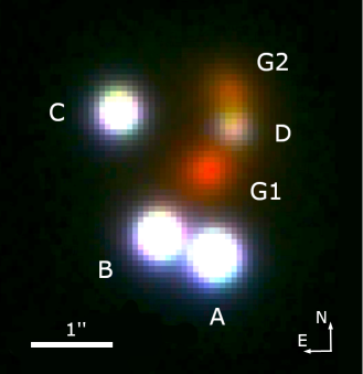
Figure 1: Color image of HE0230$-$2130 created with Magellan imaging data in the $g$-, $r$-, and $i$-band. Image courtesy of Scott Burles.

The brightest lensing galaxy (G1) is located between the multiple lensed quasar images, while the other, fainter galaxy (G2) is slightly offset to the North of image D. The maximum image separation is 2.15″. Faure et al. (2004) found a galaxy overdensity about 40″south-west of the lens and proposed that G1 and G2 are two members of a physically related galaxy group. This was later confirmed spectroscopically by Eigenbrod et al. (2006), with measured redshifts $z_{\rm G1}=0.523\pm 0.001$ and $z_{\rm G2}=0.526\pm 0.002$. The spectrum of G1 matches well that of an ETG. Anguita et al. (2008) obtained similar redshifts for G1 and G2, and found the redshift of a galaxy $\sim 17\arcsec$ north-west of image A to be $z=0.518\pm 0.002$. To estimate if G1 and G2 are potentially dynamically associated with each other we check if a typical peculiar velocity of cluster galaxies can account for the observed redshift difference of 0.003 (Harrison et al., 1974). We find that we need a peculiar velocity of around 1000 km/s, which is a typical value for cluster galaxies. Therefore G1 and G2 seem to be dynamically associated and dynamical interaction is possible to some extent.

3 Modeling method

We model HE0230$-$2130 with the software Gravitational Lens Efficient Explorer (Glee, Suyu & Halkola, 2010; Suyu et al., 2012) and its Bayesian sampling and optimization methods (simulated annealing and MCMC methods), which were automated by Ertl et al. (2023) and Schuldt et al. (2023) to minimize user interaction time. As these automated methods find the optimal sampling parameters and start new chains completely independently, we use them here to speed up the sampling of multiple different model classes.

3.1 Light and mass parametrization

To obtain accurate image positions and priors for the mass parameters of our models, we start by modeling the observed surface brightness of the quasar images and the two lensing galaxies. We select the $i$-band of the Magellan data because the lensing galaxies and quasar images are the brightest in this band.

The point-spread function (PSF) is constructed from the cutout (3.38″$\times$3.38″) of a single star in the field at (RA, dec)=(38.1548, $-$21.3166). Since the star is not necessarily located at exactly the center of the brightest pixel we interpolate and shift the cutout within fractions of a pixel to center the star. We subsample the PSF by a factor of 3 because the pixelsize of 0.069″ is large relative to the full width at half maximum of the PSF (the brightness blob of the PSF covers only a few pixels in the native data resolution). Thus we avoid numerical inaccuracies caused by an undersampled PSF. The light of the quasar images is modeled by fitting this PSF with three parameters: the $x$- and $y$-centroid and the amplitude, which is the flux of the respective image.

We parametrize the light of each lensing galaxy with one Sérsic profile (Sérsic, 1963) and fit to the quasar images with a point source which is represented by the PSF. The Sérsic profile is parametrized as

$$I_{\rm S}(x,y)=A_{\rm S}\exp\Bigg{[}-k\Bigg{\{}\Bigg{(}\frac{\sqrt{(x-x_{\rm S})^{2}+\left(\frac{y-y_{\rm S}}{q_{\text{S}}}\right)^{2}}}{r_{\rm eff}}\Bigg{)}^{\frac{1}{n_{\rm s}}}-1\Bigg{\}}\Bigg{]},$$ (1)

where $A_{\rm S}$ is the amplitude, $x_{\rm S}$ and $y_{\rm S}$ are the centroid coordinates, $q_{\rm S}$ is the axis ratio, and $n_{\rm S}$ the Sérsic index. The constant $k$ normalizes $r_{\rm eff}$ such that $r_{\rm eff}$ is the half-light radius in the direction of the semi-major axis. The light distribution is oriented with a position angle $\phi_{\rm S}$ that is measured east of north (where $\phi_{\rm S}=0^{\circ}$ corresponds to the major axis being aligned with the northern direction).

In general, we parametrize the lens mass distribution of G1 and G2 with a PL profile. The dimensionless surface mass density (or convergence) of a general PL profile is given by

$$\begin{split}\kappa_{\rm PL}(x,y)=\frac{3-\gamma}{1+q}\frac{\theta_{\rm E}^{2}}{(\theta_{\rm E}^{2}+r_{\rm c}^{2})^{\frac{3-\gamma}{2}}-r_{c}^{3-\gamma}}\\ \Big{[}(x-x_{\rm G})^{2}+\frac{(y-y_{\rm G})^{2}}{q^{2}}+r_{c}^{2}\Big{]}^{\frac{1-\gamma}{2}},\end{split}$$ (2)

where $(x_{\rm G},y_{\rm G})$ is the lens mass centroid, $q$ is the axis ratio of the elliptical mass distribution, $\theta_{\rm E}$ is the Einstein radius, $r_{\rm c}$ is the core radius, and $\gamma$ is the radial profile slope. The mass distribution is oriented with a position angle of $\phi$. For $r_{\rm c}=0\arcsec$, this reduces to a singular PL elliptical mass distribution (SPEMD; Barkana 1998). The case with $\gamma=2$ and $q=1$ corresponds to an isothermal sphere profile. We call an isothermal sphere with $r_{\rm c}=0$ a singular isothermal sphere (SIS) and with $r_{\rm c}>0$ a non-singular isothermal sphere (NIS) profile. We can account for the tidal gravitational field of surrounding objects by adding an external shear component (Keeton et al., 1997). The shear strength is calculated by $\gamma_{\rm ext}=\sqrt{\gamma_{\rm ext,1}^{2}+\gamma_{\rm ext,2}^{2}}$, with $\gamma_{\rm ext,1}$ and $\gamma_{\rm ext,2}$ as the components of the shear matrix. The lens potential for the external shear is parametrized by $\psi_{\rm ext}=\frac{1}{2}\gamma_{\rm ext}[\textrm{cos}(2\phi_{\rm ext})(x^{2}-y^{2})+2\textrm{sin}(2\phi_{\rm ext})xy]$, where $\phi_{\rm ext}$ is the shear position angle. The position angle is measured east of north, which means for $\phi_{\rm ext}=0^{\circ}$ the images are stretched vertically, and for $\phi_{\rm ext}=90^{\circ}$ the images are stretched horizontally.

3.2 Model classes

After obtaining a lens and quasar light fit, we use only the four modeled quasar image positions as constraints for our models as there is no extended structure (lensed arc) visible in the data. In addition, we assume that G1 and G2 are located at the same redshift. From this lensing configuration we would expect five images. The straight-forward approach of modeling this system by parametrizing G1 and G2 with a PL profile and adding external shear always produces one additional, unobserved quasar image about 0.5″ west of G2. Our goal is thus to find models that can produce the observed number of quasar images of HE0230$-$2130. For this we set up twelve different model parametrizations, each with varying degree of complexity and physical motivation. G1 and G2 are each described either by a singular (PL) or cored PL (cPL) profile with or without external shear. We also consider models with a singular or cored isothermal, spherical mass clump in the region of the predicted fifth images. In Tab. 1 we show an overview and description of the multiple model classes. In all models, we assume that mass follows light by fixing the mass centroids of G1 and G2 to the modeled Sérsic centroid of the galaxies. While the axis ratio of the PLs of G1 and G2 are free to vary, we set a Gaussian prior on the position angle based on the light. A detailed overview of the priors on the mass and shear parameters in each model is shown in Tab. 2.

Table 1: Overview of all twelve model classes.

Model name	description
PL1 + cPL2	G1&G2: singular PL profiles
cPL1 + cPL2 + $\gamma_{\rm ext}$	G1&G2: singular PL profiles, external shear
cPL1 + cPL2	G1: singular PL profile, G2: cored PL profile
cPL1 + cPL2 + $\gamma_{\rm ext}$	G1: singular PL profile, G2: cored PL profile, external shear
cPL1 + cPL2	G1&G2: cored PL profiles
cPL1 + cPL2 + $\gamma_{\rm ext}$	G1&G2: cored PL profiles, external shear
cPL1 + cPL2 + rSIS	G1&G2: singular PL profiles, SIS  without positional prior
cPL1 + cPL2 + rNIS	G1&G2: singular PL profiles, NIS without positional prior
cPL1 + cPL2 + rSIS	G1&G2: singular PL profiles, SIS  with positional prior
cPL1 + cPL2 + rNIS	G1&G2: singular PL profiles, NIS with positional prior
cPL1 + cPL2 + rSIS + $\gamma_{\rm ext}$	G1&G2: singular PL profiles, SIS  with positional prior, external shear
cPL1 + cPL2 + rNIS + $\gamma_{\rm ext}$	G1&G2: singular PL profiles, NIS with positional prior, external shear

Notes: The positional prior on the SIS and NIS models has a Gaussian distribution and is centred in the region where additional images were predicted.

Table 2: Model parameters and their priors.

Component	Parameter	Description	Prior	Prior range / value
	$x_{\rm G}\ [\arcsec]$	$x$-centroid	exact	fixed to best-fit light model
	$y_{\rm G}\ [\arcsec]$	$y$-centroid	exact	fixed to best-fit light model
G1/G2	$q$	axis ratio	flat	[0.6, 1]
(PL/cPL)	$\phi$ [∘]	position angle	Gaussian	centered on best-fit light model, $\sigma=10^{\circ}$
	$\theta_{\rm E}\ [\arcsec]$	Einstein radius	flat	[0.1″, 1.2″]
	$r_{\rm c}\ [\arcsec]$	core radius (cPL)	flat	[0″, 0.4″]
	$\gamma$	power-law index	Gaussian	center: 2.08, $\sigma=0.04$
	$x_{\rm sat}\ [\arcsec]$	$x$-centroid	Gaussian	center: 0.73″, $\sigma=0.14\arcsec$
satellite	$y_{\rm sat}\ [\arcsec]$	$y$-centroid	Gaussian	center: 2.17″, $\sigma=0.14\arcsec$
(rSIS/rNIS)	$\theta_{\rm E,sat}\ [\arcsec]$	Einstein radius	flat	[0.0001″, 1″]
	$r_{\rm c,sat}\ [\arcsec]$	core radius (rNIS)	flat	[0″, 1″]
external	$\gamma_{\rm ext}$	strength	flat	[0, 0.4]
shear	$\phi_{\rm ext}$ [∘]	position angle	flat	[$0^{\circ},180^{\circ}$]

Notes: We assume that mass follows light: the mass centroids of G1 and G2 are fixed to the light centroids of G1 and G2 from the best-fit light model, while the position angle of the mass has a Gaussian prior centered on the best-fit light model. The prior on the PL slope follows the SLACS lens sample (Auger et al., 2010; Shajib et al., 2021).

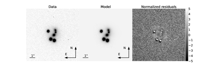
Figure 2: Observed and modeled surface brightness distribution of HE0230$-$2130 and normalized residuals in a range of $-$5$\sigma$ to 5$\sigma$.

3.3 Sampling and analysis

We sample the parameter space of each model class with MCMC chains, where each accepted point in the chain corresponds to one specific model realization. Each chain consists of 10,000,000 accepted points. Because it is difficult to incorporate into the sampling process that there is in fact not a fifth, observable image, we use the four modeled image positions as a constraint for our models and select afterwards those model realizations that predict the correct number of images. Thus we do not sample a distribution of candidate models, but a distribution where some models might fulfill the criterion of producing four observable images. This means can account not only for models that directly produce only four images, but also additional images that are too faint and hidden in the noise of the data. To robustly determine those candidate models in the MCMC chains, we compute the image positions and magnifications for each model realization using the Delaunay triangulation method. For this, the image plane is divided into triangles. The image plane triangles that, when mapped to the source plane, contain the mean weighted source position, are iteratively refined.

If a model produces only four quasar images, or if all additional images are below the flux limit of our data, we count it as a candidate model. We estimate the flux limit in the following way. Because of surface brightness conservation the minimum magnification needed for an image to be observable can be calculated via $|\mu_{\rm min}|=|\mu_{i}|\frac{K_{\rm min}}{K_{i}}$, where $\mu_{i}$ is the model predicted magnification of image $i$, $K_{i}$ is the modeled amplitude (flux) of an observed image $i$ (that can be image A, B, C or D), and $K_{\rm min}$ is the minimum amplitude for a light source to be above the flux limit. We conservatively choose the image $i$ for which the predicted magnification limit $\mu_{\rm min}$ is the lowest. We then compare this technical magnification limit with the predicted magnification of additional images. For predicted images that are very close to the center of G2 (i.e., the innermost 3 pixels $\approx 0.2\arcsec$), we obtain a separate magnification limit, which is slightly higher due to the residuals from modeling the light of G2. The priors on the mass and shear parameters in each model are tabulated in Tab. 2.

4 Results and Discussion

4.1 Light parameters of lens and source

We obtain astrometric positions of the QSO images from the lens and quasar light model by fitting the PSF to the observed quasar image light. Fig. 2 shows the results of this light fitting, by comparing the data with our model and presenting the normalized residuals in a range from $-$5$\sigma$ to 5$\sigma$. The residuals at the quasar positions are due to PSF being constructed from only one star and no corrections being performed.

In Tab. 3 we present the modeled lens light parameters from fitting one Sérsic profile to both G1 and G2. Throughout the paper we report positions in the coordinate system of CASTLES, where we take our modeled position of image A as coordinate origin.

Table 3: Lens light modeling results.

Parameter	G1	G2
$x_{\rm S}$ [″]	$-0.0801_{-0.0002}^{+0.0001}$	$0.194_{-0.002}^{+0.002}$
$y_{\rm S}$ [″]	$1.0674_{-0.0001}^{+0.0001}$	$2.052_{-0.003}^{+0.003}$
$q_{\rm S}$	$0.64_{-0.01}^{+0.01}$	$0.78_{-0.02}^{+0.02}$
$\phi_{\rm S}$ [∘]	$101_{-1}^{+1}$	$52_{-3}^{+3}$
$A_{\rm S}$	$334_{-1}^{+1}$	$199_{-1}^{+1}$
$r_{\rm eff}$ [″]	$0.422_{-0.004}^{+0.005}$	$0.424_{-0.006}^{+0.006}$
$n_{\rm S}$	$2.99_{-0.06}^{+0.07}$	$2.74_{-0.07}^{+0.08}$

Notes: G1 and G2 are each modeled with one Sérsic profile. The position angle is measured east of north. The modeled position of image A is set as the origin of the coordinate system.

G1 and G2 show regular isophotes as both can be fit well with one Sérsic profile each. Given this and the fact that we need a relative velocity between G1 and G2 of around 1000 km/s (see Sec. 1), strong dynamical interaction between the two lensing galaxies is not likely, although we cannot rule it out.

In Tab. 4 we present our best-fit modeled image positions and compare them with those measured by Gaia (Brown et al., 2018) and by CASTLES with HST data. In this table we also report measured fluxes from our models. As a magnitude zeropoint is missing for the Magellan data, we used magnitudes of stars in the field measured in the Legacy Survey DR10 to calibrate it and calculate the fluxes in the AB magnitude system. The fluxes from CASTLES are reported in the Vega system.

Table 4: Best-fit astrometric positions and fluxes of quasar images.

	A			B			C			D
	x [″]	y [″]	flux	x [″]	y [″]	flux	x [″]	y [″]	flux	x [″]	y [″]	flux
Glee	$\equiv$ 0	$\equiv$ 0	19.34 (AB)	$-$0.695	0.258	19.47 (AB)	$-$1.192	1.827	19.91 (AB)	0.261	1.610	21.59 (AB)
CASTLES	$\equiv$ 0	$\equiv$ 0	19.02 (V)	$-$0.698	0.256	19.22 (V)	$-$1.198	1.828	19.59 (V)	0.244	1.624	21.21 (V)
Gaia	$\equiv$ 0	$\equiv$ 0	$-$	$-$0.697	0.258	$-$	$-$1.198	1.832	$-$	$-$	$-$	$-$

Notes: Positional values are given in arcsec and are shifted into the CASTLES reference frame. The modeled position of image A is set as the origin of the coordinate system. There is no measured position of image D from Gaia as it is below the detection limit of the Gaia satellite. The fluxes in the Magellan $i$-band are reported in the AB magnitude system, the CASTLES fluxes are those of the HST F814W band and reported in the Vega (V) system.

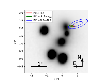
Figure 3: Modeled image of HE0230$-$2130. Plotted are the 1- and 2$\sigma$ contours of the predicted positions of the unobserved fifth quasar images in the PL1 + PL2 (red), the PL1+cPL2+$\gamma_{ext}$ (green), and the PL1+PL2+rNIS (blue) model class. These predicted fifth quasar images would be above the detection threshold, but are not observed in the imaging data.

We find that our modeled image positions agree within 6 mas in $x$-direction and 5 mas in $y$-direction with Castles and Gaia. We exclude only image D in this comparison, which has a bigger offset to the position for Castles because it is the faintest image and partially blended with the light of G2.

4.2 Candidate models

We present the final mass and shear parameters of all model classes in Tab. 7. We tabulate both the distributions of parameters for the full chain and the candidate model realizations. Tab. 5 shows an overview of our results. The modeled position of image A is set as the origin of the coordinate system.

Table 5: Overview of the candidate fraction of all model classes.

Model	correct # of images	$f_{\rm cand}$
PL1 + cPL2	$\times$	0%
cPL1 + cPL2 + $\gamma_{\rm ext}$	$\times$	0%
cPL1 + cPL2	$\times$	0%
cPL1 + cPL2 + $\gamma_{\rm ext}$	$\checkmark$	0.26%
cPL1 + cPL2	$\times$	0%
cPL1 + cPL2 + $\gamma_{\rm ext}$	$\checkmark$	0.26%
cPL1 + cPL2 + rSIS	$\times$	0%
cPL1 + cPL2 + rNIS	$\times$	0%
cPL1 + cPL2 + rSIS	$\checkmark$	0.03%
cPL1 + cPL2 + rNIS	$\checkmark$	1.7%
cPL1 + cPL2 + rSIS + $\gamma_{\rm ext}$	$\checkmark$	0.4%
cPL1 + cPL2 + rNIS + $\gamma_{\rm ext}$	$\checkmark$	12%

Notes: Candidate models are model realizations that predict four instead of five quasar images, or where additional images are below the flux limit of the data. $f_{\rm cand}$ is the weighted percentage of candidate model realizations in the MCMC chain. In this computation we take the statistical weights of the MCMC chain into account.

Six of the twelve model classes we considered can produce models that match the observed image multiplicity. We find that the simplest models, where G1 and G2 are parametrized by a singular PL profile with or without external shear, consistently produce exactly one additional image as expected from this lensing configuration. These additional images are located about 0.5″west of G2, with a magnification that should make it observable. Fig. 3 shows the 1- and 2-$\sigma$ contours of the predicted positions of this fifth image in the PL1 + PL2, the PL1+cPL2+$\gamma_{ext}$, and the PL1+PL2+rNIS model classes.

In the class PL1 + cPL2 + $\gamma_{\rm ext}$, 0.26% of the models produce the correct, observed image multiplicity, while for PL1 + cPL2 (same parameterization for G1 and G2 but without external shear) there are no models that match the observation. Similarly, for the model class cPL1 + cPL2 + $\gamma_{\rm ext}$, 0.26% of the models fit the observations, while there are no candidate models in cPL1 + cPL2.

A similar effect might be produced by placing an SIS or NIS mass distribution close to the saddle point of the fifth image on the lens plane. This mass can be interpreted as DM substructure or an unobservable, dark galaxy. We find that by simply placing a SIS or NIS clump without positional prior, they tend to move away from the region close to the saddle point and predominantly end up west of image D. Thus, these two model classes are unable to suppress the fifth image.

To keep the mass clumps closer to G2, we set a Gaussian prior on the SIS and NIS centroids. We call these profiles “restricted” SIS/NIS, in short rSIS and rNIS. G1 and G2 are parametrized as singular PL profiles. Of the PL1 + PL2 + rSIS models, 0.03% do not predict a fifth image. This is also the case for 1.7% of the PL1 + PL2 + rNIS models.

Finally, we analyze the PL1 + PL2 + rSIS and PL1 + PL2 + rNIS models with the presence of external shear. We find that this significantly increases the fraction of candidates to 0.4% in the PL1 + PL2 + rSIS+$\gamma_{\rm ext}$ case, and to 12% for the PL1 + PL2 + rNIS+$\gamma_{\rm ext}$ class.

In the following, we describe and interpret in detail the results of each model class that produces the observed four images.

4.2.1 PL1 + cPL2 + $\gamma_{\rm ext}$

In this model class, G1 is described by a singular PL profile, while G2 is parametrized as a cored PL profile. Galaxies that are part of clusters often exhibit a core, while for isolated field galaxies a core is not common. An additional external shear component is necessary to reproduce the observed image multiplicity as the PL1 + cPL2 model class predicts always an additional image. By adding a core to the mass distribution of G2, the saddle point of the fifth image merges with the maximum of G2. In Fig. 4, we plot the Fermat potential of two non-candidate and one candidate model, that is, before and after merging of the saddle with the maximum. The difference between candidate and non-candidate is also evident in the source position with respect to the caustic curves in the source plane: as the radial caustic shrinks and changes in shape, the source crosses the radial caustic into the shaded green region, and the image multiplicity of this model changes. Furthermore, the Fermat potential is flattened in the vicinity of the vanished image.

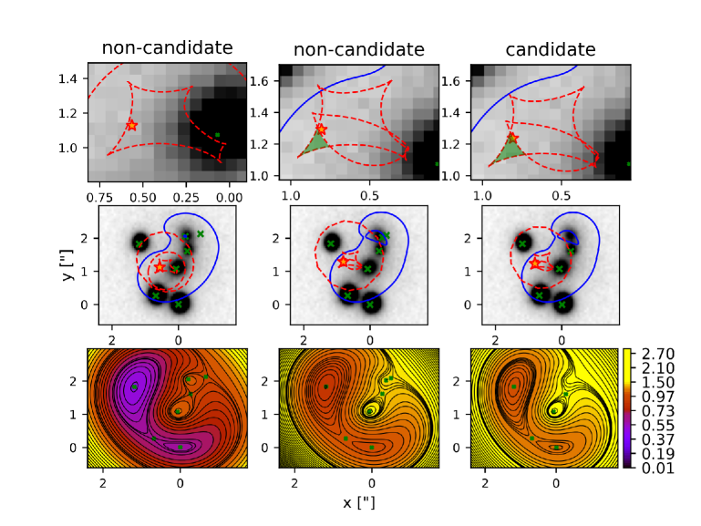
Figure 4: Change of critical curves and caustics between non-candidate models (left and middle columns) and one candidate model (right column). The top and middle row show the critical curves (blue, solid lines) and caustic curves (red, dashed lines). The bottom row shows the Fermat potential and contours with the color scale in units of ${\textrm{arcsec}}^{2}$. As the core radius of G2 increases and the source position crosses the radial caustic into the shaded green region, the time-delay saddle point associated with the fifth images merges with the maximum of G2 and the fifth image disappears. The source position is plotted as a yellow star. In each panel the predicted image positions are shown as green crosses.

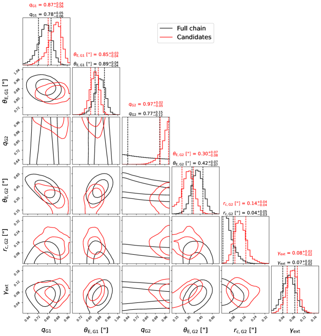
Figure 7: PL1 + cPL2 + $\gamma_{\rm ext}$: posterior distributions for several lens mass parameters of the power-law profile (see Sec. 3) and the external shear strength. We show the distributions for candidate models (i.e., models that predict four observable quasar images) in red, and the distribution of the whole MCMC chain is plotted in black. The two contours show the 1- and 2$\sigma$ credible regions. The one-dimensional histograms show the marginalized posterior distribution for the selected mass parameters, and the vertical lines mark the 1$\sigma$ confidence intervals.

In Fig 7 we show the posterior distribution of selected lens mass and shear parameters. The distributions of candidate models are plotted in red contours, the distribution of the whole chain (i.e., both candidate and non-candidate models) are plotted in black contours. We find that candidate models have a very round mass distribution of G2 with $q_{\rm G2,cand}=0.97_{-0.05}^{+0.02}$, while the general distribution of the chain is more uniformly distributed over the whole prior range: $q_{\rm G2,all}=0.77_{-0.12}^{+0.15}$. Similarly, the general distribution of $r_{\rm c,G2}$ is skewed towards a vanishing core radius (i.e., a singular PL profile). In order to produce only four images, a core radius of $r_{\rm c,G2,cand}=(0.14_{-0.04}^{+0.04})\arcsec$ is needed. The candidate models are all found in the tail of the distribution. The shear strength of candidate models is $\gamma_{\rm ext,cand}=0.08_{-0.02}^{+0.02}$. This is a typical value for quadruply lensed quasars as shown by Luhtaru et al. 2021.

4.2.2 cPL1 + cPL2 + $\gamma_{\rm ext}$

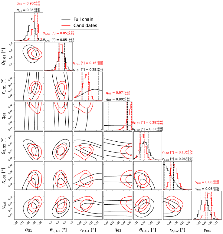
Figure 8: Posterior distributions for the cPL1 + cPL2 + $\gamma_{\rm ext}$ model class.

Now we parametrize both G1 and G2 with a cored PL profile. As for the PL1 + cPL2 + $\gamma_{\rm ext}$ case, we need external shear to reproduce the correct image multiplicity. The mechanism by which the fifth image is eliminated is the same as in the PL1 + cPL2 + $\gamma_{\rm ext}$ model class: the saddle point of the fifth image merges with the maximum of G2. We show the posterior distributions of all models compared to the candidates in Fig 8. Again, a clear tendency of the candidate models is a high $q_{\rm G2,cand}$ compared the more uniform, general distribution. The distribution of candidate core radii are $r_{\rm c,G1,cand}=(0.16_{-0.06}^{+0.04})\arcsec$ and $r_{\rm c,G2,cand}=(0.13_{-0.04}^{+0.04})\arcsec$, respectively. The external shear has a distribution of $\gamma_{\rm ext,cand}=0.08_{-0.02}^{+0.01}$.

4.2.3 PL1 + PL2 + rSIS and PL1 + PL2 + rNIS

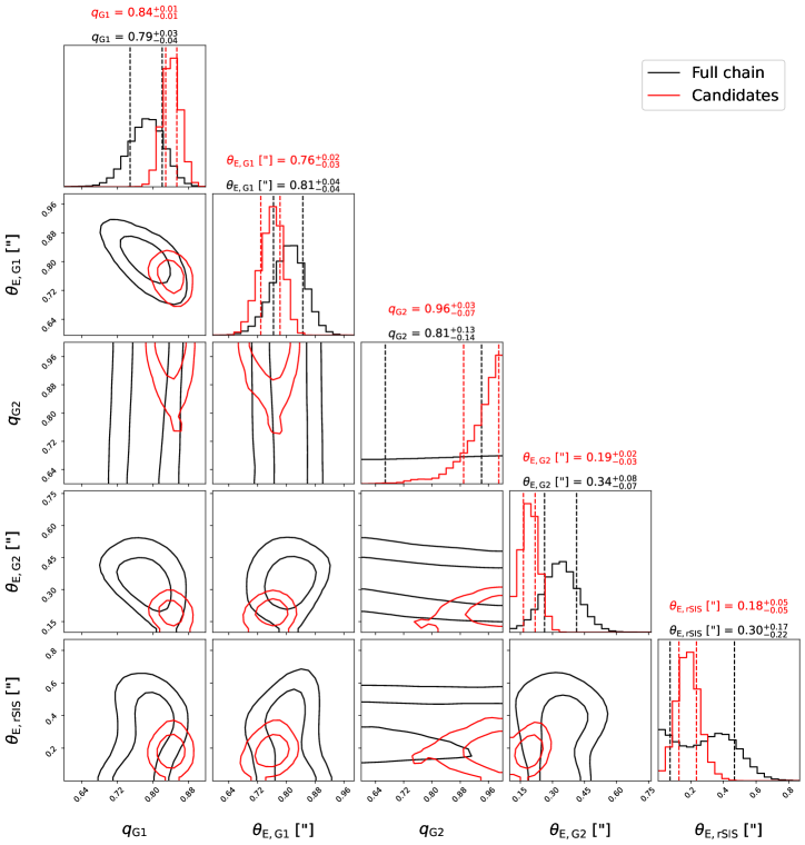
Figure 9: Posterior distributions for the PL1 + PL2 + rSIS model class.

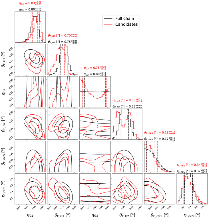
Figure 10: Posterior distributions for the PL1 + PL2 + rNIS model class.

The physical motivation behind the model classes with an SIS or NIS profile is to simulate a dark mass distribution in the plane of the lensing galaxies, for instance, DM substructure or a dwarf galaxy. The PL1 + PL2 + SIS and PL1 + PL2 + NIS model classes can not reproduce the correct number of images as the centroids of the mass clumps are moving away from the critical region where the saddle of the fifth image can be merged with the maximum of G2. We assume a Gaussian prior on the centroid of the SIS/NIS clump to keep it close to the critical region shown in Fig 3. As mentioned earlier, we call these “restricted” SIS and NIS profiles “rSIS” and “rNIS”. While the PL1 + PL2 + SIS and PL1 + PL2 + NIS model class do not predict models with only four images, 0.03% of PL1 + PL2 + rSIS models produce no fifth image. For the PL1 + PL2 + rNIS model class the percentage is 1.7%. We can see in Fig 9 and Fig 10, that, with the presence of an additional mass component close to G2, the Einstein radius $\theta_{\rm E,G2}$ decreases. The PL1 + PL2 + rSIS candidate models predict an especially low Einstein radius of G2 with $\theta_{\rm E,G2,cand}=(0.20_{-0.03}^{+0.02})\arcsec$, while it is higher for the candidates in the rNIS model: $\theta_{\rm E,G2,cand}=(0.33_{-0.14}^{+0.11})\arcsec$. The Einstein radius of the rSIS in candidate models is $\theta_{\rm E,rSIS,cand}=(0.18_{-0.05}^{+0.05})\arcsec$. The PL1 + PL2 + rNIS candidates have an rNIS Einstein radius of $\theta_{\rm E,rNIS,cand}=(0.13_{-0.09}^{+0.12})\arcsec$ and a core radius $r_{\rm c,rNIS,cand}=(0.34_{-0.13}^{+0.19})\arcsec$.

4.2.4 PL1 + PL2 + rSIS + $\gamma_{\rm ext}$ and PL1 + PL2 + rNIS + $\gamma_{\rm ext}$

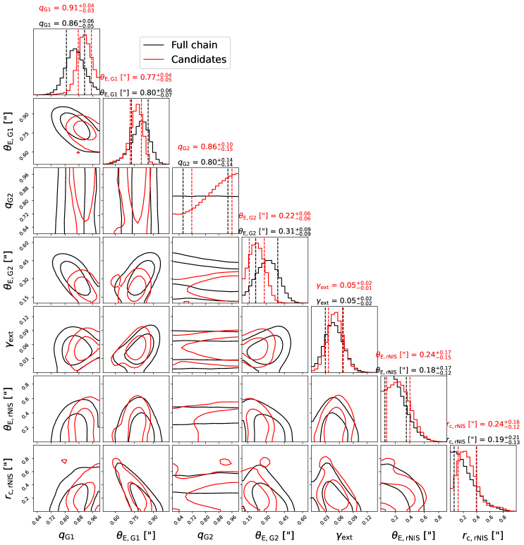
Figure 12: Posterior distributions for the PL1 + PL2 + rNIS + $\gamma_{\rm ext}$ model class.

By adding external shear to the PL1 + PL2 + rSIS and PL1 + PL2 + rNIS model classes, the fraction of candidate models increases substantially. The effect of adding external shear to our models can be seen in the corner plots in Fig. 10 and 12. The physical meaning of external shear has recently been challenged, as shear values inferred from strong lensing are inconsistent with independent measurements from, e.g., weak lensing (Etherington et al., 2023). The fact that the inclusion of external shear in our models generally increases the candidate fraction thus could mean that there is some complexity in this lensing system that cannot be accounted for with just two (cored) PL profiles for G1 and G2. This is not surprising as G1 and G2 are possibly embedded in a common DM halo. In particular, 12% of models of the PL1 + PL2 + rNIS + $\gamma_{\rm ext}$ class produces the correct number of images. The 1- and 2-$\sigma$ contours of the PL1 + PL2 + rNIS + $\gamma_{\rm ext}$ centroids, are plotted on the modeled image in Fig. 5. This shows that the mass clumps in models with the correct image multiplicity are located about 0.5″north-west of G2. The posterior distributions in Fig 12 show that the PL1 + PL2 + rNIS + $\gamma_{\rm ext}$ candidates have an rNIS Einstein radius of $\theta_{\rm E,rNIS+\gamma_{\rm ext},cand}=(0.24_{-0.16}^{+0.17})\arcsec$ and a core radius $r_{\rm c,rNIS+\gamma_{\rm ext},cand}=(0.24_{-0.12}^{+0.16})\arcsec$. The external shear strength is $\gamma_{\rm ext,cand}=0.05_{-0.02}^{+0.02}$.

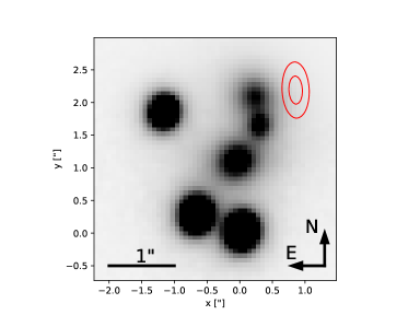
Figure 5: 1- and 2$\sigma$ contours of the mass centroid of the candidate rNIS clumps in the PL1 + PL2 + rNIS model class. These candidate models predict only four quasar images, or additional images that are too faint to be observed (i.e., below the flux limit of the data).

4.3 Model comparison

As there are multiple model classes that are able to produce the correct number of observed images, we investigate now which of the model classes is more likely by comparing their likelihoods. Rather than using the minimum $\chi^{2}_{\rm im}$ for the comparison, we calculate the Bayesian Information Criterion (BIC) to weigh the model according to both their complexity and goodness of fit. The BIC is defined as

$$\textrm{BIC}=k\ln(N_{\rm data})-2\ln(\hat{\mathcal{L}}),$$ (3)

where $k$ is the number of free parameters, $N_{\rm data}$ is the number of data points, and $\hat{\mathcal{L}}$ is the maximum likelihood of the candidate models. The relative probability of a model M with BIC compared to the most likely model $\textrm{M}^{*}$ with $\textrm{BIC}^{*}$ is

$$p(\textrm{M})/p(\textrm{M}^{*})=\textrm{exp}(-\frac{\textrm{BIC}-\textrm{BIC}^{*}}{2})\times\frac{f_{\rm cand,M}}{f_{\rm cand,{M}^{*}}},$$ (4)

where $f_{\rm cand}$ is the weighted fraction of candidate models in the MCMC chain. In terms of free parameters $k$ we have the free lens galaxy model parameters + 2 for the source position. Because we calculate the flux limit that is specific for each model class and which we use to select candidate models, we count the source intensity as an additional free parameter and the image amplitude $K_{i}$ (see Sec.3.3) as an additional data point to the 8 data points from the four image positions. Additionally, we count the Gaussian priors as both free parameter and data point. In Tab. 6 we present the BIC values and relative probabilities of our six candidate models.

Table 6: Bayesian comparison of candidate model classes.

model	$k$	$N_{\rm data}$	$f_{\rm cand}$	min. $\chi^{2}_{\rm im}$	BIC	$p(\textrm{M})/p(\textrm{M}^{*})$
cPL1 + cPL2 + $\gamma_{\rm ext}$	14	13	0.26%	1.32	37.23	0.94
cPL1 + cPL2 + $\gamma_{\rm ext}$	15	13	0.26%	0.54	39.01	0.38
cPL1 + cPL2 + rSIS	14	15	0.03%	1.60	39.51	0.04
cPL1 + cPL2 + rNIS	15	15	1.7%	0.12	40.80	1
cPL1 + cPL2 + rSIS + $\gamma_{\rm ext}$	16	15	0.4%	0.13	43.46	0.07
cPL1 + cPL2 + rNIS + $\gamma_{\rm ext}$	17	15	12%	0.03	46.07	0.53

Notes: $k$ is the number of free parameters, $N_{\rm data}$ is the number of data points, and $f_{\rm cand}$ is the weighted fraction of candidate models in the MCMC chain. The relative probability $p(\textrm{M})/p(\textrm{M}^{*})$ is calculated via Eq. 4 and then renormalized.

The most likely model class is PL1 + PL2+ rNIS, which is slightly favored over the model class PL1 + cPL2 + $\gamma_{\rm ext}$, which has a relative probability of 94%. Although cPL1 + cPL2 + $\gamma_{\rm ext}$ has a lower $\chi^{2}_{\rm im}$ and a similar fraction of candidates compared to PL1 + cPL2 + $\gamma_{\rm ext}$, the latter is simpler in terms of model complexity (with a fewer number of free parameters) and is thus favored by the BIC.

4.4 Plausibility of inferred parameter values

To check the plausibility of the model parameter values of our two favored model classes, we estimate the mass-to-light ratio $\frac{M}{L}$ of G1 and G2 for both classes. We obtain the luminosity $L$ by numerically integrating the modeled Sérsic light profile (see Eq. 1) within the effective radius $r_{\rm eff}$. From the integrated fluxes we obtain apparent magnitudes $m_{\rm G1,AB}=20.39$ and $m_{\rm G2,AB}=20.79$, which convert to $L_{\rm G1}=7.45\times 10^{9}L_{\odot}$ and $L_{\rm G2}=5.17\times 10^{9}L_{\odot}$. We infer the mass by integrating the $\kappa_{\rm PL}$ profile of the respective model class within the same effective radius as the light. From a distribution of candidate models we find $M_{\rm G1,cPL2}=8.1^{+1.0}_{-1.0}\times 10^{10}M_{\odot}$ and $M_{\rm G2,cPL2}=3.5^{+0.5}_{-0.5}\times 10^{10}M_{\odot}$ for the PL1+cPL2+$\gamma_{\rm ext}$ model class, and $M_{\rm G1,rNIS}=7.5^{+0.5}_{-0.4}\times 10^{10}M_{\odot}$ and $M_{\rm G2,rNIS}=2.4^{+1.9}_{-0.8}\times 10^{10}M_{\odot}$ for the PL1+PL2+rNIS model class. For G1 we thus find mass-to-light ratios of $\Big{(}\frac{M}{L}\Big{)}_{\rm G1,cPL2}=10.9^{+1.4}_{-1.3}$ and $\Big{(}\frac{M}{L}\Big{)}_{\rm G1,rNIS}=10.0^{+0.6}_{-0.6}$. This is on the upper range of expected values for ETGs in the observed $i$-band, and is thus plausible especially since we did not explicitly model a galaxy group DM halo and some of the calculated mass of G1 could be attributed to the group halo. For G2 we find $\Big{(}\frac{M}{L}\Big{)}_{\rm G2,cPL2}=6.7^{+1.0}_{-1.0}$ and $\Big{(}\frac{M}{L}\Big{)}_{\rm G2,rNIS}=4.7^{+3.7}_{-1.6}$. Both G1 and G2 fall into the expected range for mass-to-light ratios.

4.5 Detection of DM substructure?

Our preferred model class PL1+Pl2+rNIS implies the presence of a mass clump about 0.5″ north-west of G2. We now investigate the nature of the predicted rNIS clumps in the PL1 + PL2 + rNIS model class by calculating their mass enclosed within the Einstein radius. For an NIS profile, the enclosed mass within its Einstein radius $\theta_{\rm E,NIS}$ is

$$M_{\rm NIS}=\pi\theta_{\rm E,NIS}^{2}D_{\rm d}^{2}\Sigma_{\rm crit}=\frac{c^{2}}{4G}\theta_{\rm E,NIS}^{2}\frac{D_{\rm d}D_{\rm s}}{D_{\rm ds}},$$ (5)

where $\Sigma_{\rm crit}$ is the critical surface mass density, and the distances $D_{\rm d}$, $D_{\rm s}$ and $D_{\rm ds}$ are the angular diameter distance to the lens galaxy, to the source galaxy, and between the deflector and source galaxy, respectively.

We show the distribution of $M_{\rm rNIS}$ of all candidate models in the chain on a logarithmic scale in Fig. 6. It spans a mass range of $\sim 4\times 10^{3}-1\times 10^{11}M_{\odot}$. 18% of all candidate models predict $10^{6}M_{\odot}\leq M_{\rm rNIS}\leq 10^{9}M_{\odot}$, which is the range of predicted masses for DM substructure or dark dwarf-galaxies (Dalal & Kochanek, 2001; Simon & Geha, 2007; Diemand et al., 2008; Vegetti et al., 2012). $\sim$69% of all candidate models predict $M_{\rm rNIS}\leq 10^{10}M_{\odot}$. We conclude that it is possible that some dark matter substructure is present close to G2, changing the landscape of critical curves and caustics, and ultimately eliminating the fifth quasar image.

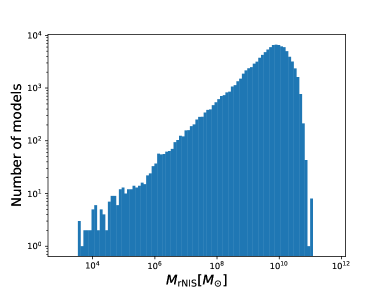
Figure 6: Logarithmic distribution of the masses of rNIS clumps (in solar masses) in the candidate models of the PL1 + PL2 + rNIS + $\gamma_{\rm ext}$ model class.

5 Summary

We modeled and analyzed the strongly lensed quasar HE0230$-$2130 using ground-based imaging data from the Magellan telescope. This lensing system shows a peculiar configuration with two lensing galaxies at similar redshift and four quasar images. The lensing galaxies are possibly part of a larger galaxy group and it is possible that the two lensing galaxies are dynamically associated or are embedded in an overall DM halo. As we expect five quasar images for such a lensing configuration, our aim is to find models that produce only four images. After we obtained the image positions by modeling the lens and quasar light in the observed image, we use them to constrain the mass parameters of our models. The straight-forward approach of modeling both lens galaxies with a singular PL profile agrees with our expectations and always results in one additional predicted image, which is not observable in the data. We test a dozen different model parametrizations where we add core radii to the PL profiles describing G1 and G2, and/or we add a singular or cored isothermal sphere profile at the same redshift as G1 and G2, mimicking a dark mass distribution. We find that introducing a core to G2, or to G1 and G2 can explain the missing image, as well as a cored or singular isothermal sphere close to the predicted position of the missing image. In all of these cases the saddle of the missing image merges with the maximum of G2, such that only four observable quasar images remain. All model classes consistently predict an external shear strength between 0.06 and 0.08. Adding external shear to the models generally increases the candidate fraction. This could mean that this system is potentially not dynamically relaxed as external shear parameter is recently thought to compensate for missing model complexity. We compare the likelihoods of each candidate model class with the BIC and take into account the fraction of candidate models. The most likely model class is cPL1 + cPL2 + rNIS, where 1.7% of all models produce the correct number of images.

We conclude that we found models that can describe this peculiar lensing system. The most likely explanation is the PL1 + PL2 + rNIS parametrization, which suggests the presence an undetected, dark mass clump. 18% of those candidate models predict an NIS mass of $10^{6}M_{\odot}\leq M_{\rm NIS}\leq 10^{9}M_{\odot}$, which is the predicted mass range of DM substructure or dark dwarf galaxies. Almost equally likely is the presence of a core in G2 in combination with external shear. Follow-up high-resolution and high-signal-to-noise-ratio imaging observations, which could display the quasar host galaxy as arcs or give us a better view of the region around G2, would help to further constrain our models and shed light on the unusual nature of HE0230$-$2130.

Appendix A Final model parameter values of all candidate model classes

Table 7: Final model parameter values of all candidate model classes.

Parameter description	Parameter		Model class
			PL1 + cPL2 + $\gamma_{\rm ext}$	cPL1 + cPL2 + $\gamma_{\rm ext}$	PL1 + PL2 + rSIS	PL1 + PL2 + rNIS	PL1 + PL2 + rSIS + $\gamma_{\rm ext}$	PL1 + PL2 + rNIS + $\gamma_{\rm ext}$
G1 lens mass (power-law)
axis-ratio	$q_{\rm G1}$	full chain	${0.78}^{+0.05}_{-0.06}$	${0.85}^{+0.03}_{-0.04}$	${0.79}^{+0.03}_{-0.04}$	${0.80}^{+0.03}_{-0.04}$	${0.83}^{+0.04}_{-0.05}$	${0.86}^{+0.06}_{-0.05}$
		candidates	${0.87}^{+0.04}_{-0.06}$	${0.90}^{+0.03}_{-0.03}$	${0.84}^{+0.01}_{-0.02}$	${0.83}^{+0.02}_{-0.05}$	${0.90}^{+0.03}_{-0.03}$	${0.91}^{+0.04}_{-0.04}$
position angle	$\phi_{\rm G1}$ [°]	full chain	${118}^{+8}_{-7}$	${109}^{+8}_{-8}$	${107}^{+13}_{-11}$	${91}^{+7}_{-7}$	${104}^{+10}_{-10}$	${101}^{+10}_{-10}$
		candidates	${122}^{+12}_{-9}$	${113}^{+9}_{-9}$	${112}^{+4}_{-3}$	${89}^{+7}_{-8}$	${104}^{+9}_{-9}$	${101}^{+11}_{-10}$
Einstein radius	$\theta_{\rm E,G1}\ [^{\prime\prime}]$	full chain	${0.89}^{+0.04}_{-0.04}$	${0.85}^{+0.04}_{-0.05}$	${0.81}^{+0.04}_{-0.04}$	${0.75}^{+0.04}_{-0.04}$	${0.86}^{+0.04}_{-0.04}$	${0.80}^{+0.06}_{-0.07}$
		candidates	${0.85}^{+0.03}_{-0.04}$	${0.85}^{+0.03}_{-0.03}$	${0.76}^{+0.02}_{-0.03}$	${0.70}^{+0.05}_{-0.06}$	${0.81}^{+0.02}_{-0.03}$	${0.77}^{+0.04}_{-0.05}$
core radius	$r_{\rm c,G1}\ [^{\prime\prime}]$	full chain	$-$	${0.25}^{+0.10}_{-0.13}$	$-$	$-$	$-$	$-$
		candidates	$-$	${0.16}^{+0.04}_{-0.06}$	$-$	$-$	$-$	$-$
power-law index	$\gamma_{\rm G1}$	full chain	${1.97}^{+0.14}_{-0.15}$	${2.07}^{+0.16}_{-0.15}$	${1.96}^{+0.23}_{-0.21}$	${2.17}^{+0.14}_{-0.14}$	${2.14}^{+0.15}_{-0.15}$	${2.19}^{+0.14}_{-0.14}$
		candidates	${1.88}^{+0.14}_{-0.15}$	${2.01}^{+0.16}_{-0.14}$	${1.66}^{+0.08}_{-0.07}$	${2.13}^{+0.20}_{-0.27}$	${2.04}^{+0.14}_{-0.15}$	${2.13}^{+0.14}_{-0.13}$
G2 lens mass (power-law)
axis-ratio	$q_{\rm G2}$	full chain	${0.77}^{+0.15}_{-0.12}$	${0.80}^{+0.14}_{-0.14}$	${0.81}^{+0.13}_{-0.14}$	${0.80}^{+0.14}_{-0.14}$	${0.79}^{+0.14}_{-0.13}$	${0.80}^{+0.14}_{-0.14}$
		candidates	${0.97}^{+0.02}_{-0.05}$	${0.97}^{+0.03}_{-0.05}$	${0.96}^{+0.03}_{-0.07}$	${0.75}^{+0.20}_{-0.12}$	${0.94}^{+0.05}_{-0.09}$	${0.86}^{+0.10}_{-0.15}$
position angle	$\phi_{\rm G2}$ [°]	full chain	${50}^{+10}_{-10}$	${51}^{+10}_{-10}$	${52}^{+10}_{-10}$	${52.0}^{+10}_{-10}$	${52}^{+9}_{-9}$	${52}^{+10}_{-10}$
		candidates	${53}^{+8}_{-10}$	${54}^{+11}_{-11}$	${55}^{+10}_{-10}$	${52}^{+9}_{-10}$	${54}^{+10}_{-10}$	${53}^{+10}_{-10}$
Einstein radius	$\theta_{\rm E,G2}\ [^{\prime\prime}]$	full chain	${0.42}^{+0.07}_{-0.07}$	${0.32}^{+0.08}_{-0.08}$	${0.34}^{+0.08}_{-0.07}$	${0.33}^{+0.07}_{-0.07}$	${0.36}^{+0.07}_{-0.09}$	${0.31}^{+0.09}_{-0.10}$
		candidates	${0.3}^{+0.07}_{-0.08}$	${0.28}^{+0.05}_{-0.05}$	${0.20}^{+0.02}_{-0.03}$	${0.33}^{+0.11}_{-0.14}$	${0.29}^{+0.04}_{-0.05}$	${0.22}^{+0.06}_{-0.06}$
core radius	$r_{\rm c,G2}\ [^{\prime\prime}]$	full chain	${0.04}^{+0.05}_{-0.03}$	${0.06}^{+0.07}_{-0.04}$	$-$	$-$	$-$	$-$
		candidates	${0.14}^{+0.04}_{-0.04}$	${0.13}^{+0.04}_{-0.04}$	$-$	$-$	$-$	$-$
power-law index	$\gamma_{\rm G2}$	full chain	${2.26}^{+0.14}_{-0.13}$	${2.18}^{+0.14}_{-0.14}$	${2.01}^{+0.12}_{-0.11}$	${2.16}^{+0.15}_{-0.14}$	${2.12}^{+0.15}_{-0.15}$	${2.12}^{+0.15}_{-0.14}$
		candidates	${2.26}^{+0.17}_{-0.14}$	${2.23}^{+0.14}_{-0.14}$	${1.89}^{+0.06}_{-0.08}$	${2.01}^{+0.13}_{-0.1}$	${1.94}^{+0.07}_{-0.08}$	${2.02}^{+0.12}_{-0.11}$

Table 8: Table 7 continued.

Parameter description	Parameter		Model class
			PL1 + cPL2 + $\gamma_{\rm ext}$	cPL1 + cPL2 + $\gamma_{\rm ext}$	PL1 + PL2 + rSIS	PL1 + PL2 + rNIS	PL1 + PL2 + rSIS + $\gamma_{\rm ext}$	PL1 + PL2 + rNIS + $\gamma_{\rm ext}$
satellite mass (rSIS/rNIS)
$x$-centroid	$x_{\rm sat}\ [^{\prime\prime}]$	full chain	$-$	$-$	${0.84}^{+0.17}_{-0.16}$	${0.83}^{+0.12}_{-0.13}$	${0.71}^{+0.14}_{-0.14}$	${0.71}^{+0.13}_{-0.14}$
		candidates	$-$	$-$	${0.79}^{+0.14}_{-0.19}$	${0.84}^{+0.14}_{-0.12}$	${0.77}^{+0.11}_{-0.11}$	${0.69}^{+0.11}_{-0.12}$
$y$-centroid	$y_{\rm sat}\ [^{\prime\prime}]$	full chain	$-$	$-$	${2.22}^{+0.15}_{-0.14}$	${2.12}^{+0.13}_{-0.13}$	${2.21}^{+0.14}_{-0.14}$	${2.21}^{+0.13}_{-0.13}$
		candidates	$-$	$-$	${2.47}^{+0.10}_{-0.10}$	${2.02}^{+0.19}_{-0.34}$	${2.36}^{+0.11}_{-0.11}$	${2.32}^{+0.10}_{-0.10}$
Einstein radius	$\theta_{\rm E,sat}\ [^{\prime\prime}]$	full chain	$-$	$-$	${0.30}^{+0.17}_{-0.23}$	${0.17}^{+0.15}_{-0.12}$	${0.23}^{+0.15}_{-0.12}$	${0.18}^{+0.17}_{-0.12}$
		candidates	$-$	$-$	${0.18}^{+0.05}_{-0.05}$	${0.13}^{+0.12}_{-0.09}$	${0.22}^{+0.08}_{-0.07}$	${0.24}^{+0.17}_{-0.16}$
core radius	$r_{\rm c,sat}\ [^{\prime\prime}]$	full chain	$-$	$-$	$-$	${0.37}^{+0.12}_{-0.12}$	$-$	${0.19}^{+0.21}_{-0.13}$
		candidates	$-$	$-$	$-$	${0.34}^{+0.19}_{-0.13}$	$-$	${0.24}^{+0.16}_{-0.12}$
external shear
strength	$\gamma_{\rm ext}$	full chain	${0.07}^{+0.02}_{-0.02}$	${0.06}^{+0.02}_{-0.02}$	$-$	$-$	${0.06}^{+0.02}_{-0.02}$	${0.05}^{+0.02}_{-0.02}$
		candidates	${0.08}^{+0.02}_{-0.02}$	${0.08}^{+0.01}_{-0.02}$	$-$	$-$	${0.07}^{+0.02}_{-0.02}$	${0.05}^{+0.02}_{-0.02}$
position angle	$\phi_{\rm ext}$ [°]	full chain	${31}^{+10}_{-8}$	${37}^{+7}_{-8}$	$-$	$-$	${33}^{+6}_{-7}$	${25}^{+16}_{-10}$
		candidates	${29}^{+8}_{-5}$	${32}^{+4}_{-3}$	$-$	$-$	${29}^{+3}_{-4}$	${18}^{+12}_{-8}$

Appendix B Corner plots for candidate model classes

In this Appendix, we present constraints on a selection of mass and external shear parameters for each candidate model class. The distributions of candidates are plotted in red over the general distribution of the complete chain, which is colored in black.

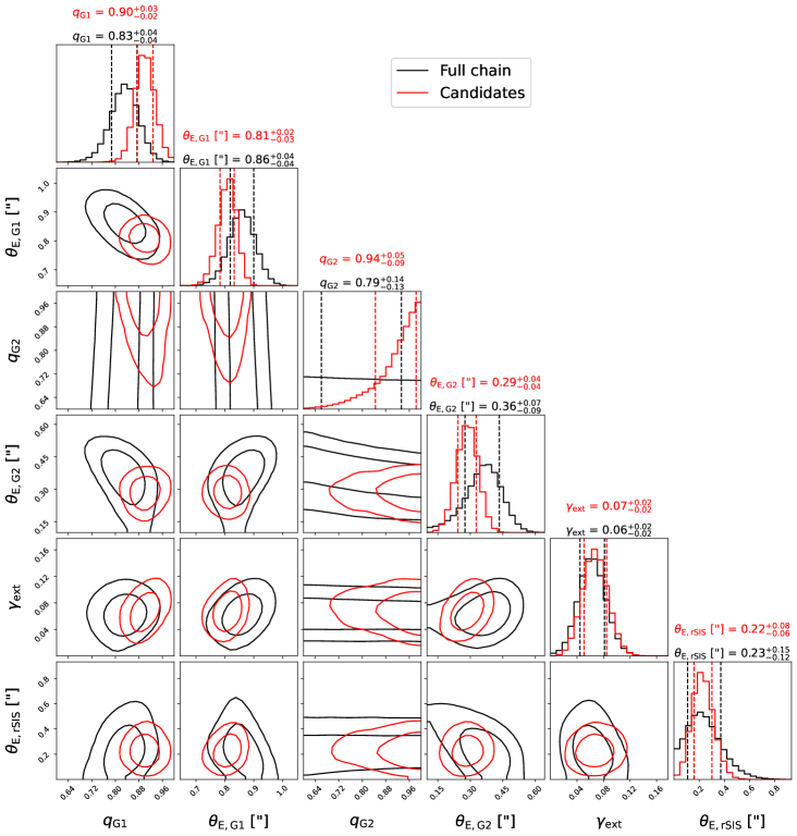
Figure 11: Posterior distributions for the PL1 + PL2 + rSIS + $\gamma_{\rm ext}$ model class.