Twinning Commercial Radio Waveforms in the Colosseum Wireless Network Emulator

Abstract.

Because of the ever-growing amount of wireless consumers, spectrum-sharing techniques have been increasingly common in the wireless ecosystem, with the main goal of avoiding harmful interference to coexisting communication systems. This is even more important when considering systems, such as nautical and aerial fleet radars, in which incumbent radios operate mission-critical communication links. To study, develop, and validate these solutions, adequate platforms, such as the Colosseum wireless network emulator, are key as they enable experimentation with spectrum-sharing heterogeneous radio technologies in controlled environments. In this work, we demonstrate how Colosseum can be used to twin commercial radio waveforms to evaluate the coexistence of such technologies in complex wireless propagation environments. To this aim, we create a high-fidelity spectrum-sharing scenario on Colosseum to evaluate the impact of twinned commercial radar waveforms on a cellular network operating in the CBRS band. Then, we leverage IQ samples collected on the testbed to train a machine learning agent that runs at the base station to detect the presence of incumbent radar transmissions and vacate the bandwidth to avoid causing them harmful interference. Our results show an average detection accuracy of 88%, with accuracy above 90% in SNR regimes above $0$ dB and SINR regimes above $-20$ dB, and with an average detection time of $137$ ms.

1. Introduction

The evolution of wireless technology has resulted in the ever-increasing complexity of wireless systems design. New generations of wireless networks have become more challenging to manage due to requirements necessitating optimal sharing of valuable resources between expanding sets of users. These challenges force researchers to think beyond traditional model-based approaches that are often limited to a specific problem scope and move toward Artificial Intelligence (AI) solutions that offer superior performance in a wider range of conditions (e.g., channel conditions in this context) thanks to their data-driven nature.

The advancements of AI-based solutions pave the way for more efficient use of the limited Radio Frequency (RF) spectrum, enabling multiple wireless systems to coexist harmoniously and cater to the growing demands of the digital era. Besides these benefits, challenges still exist regarding the potential interference between wireless networks that share the same spectrum. These mostly concern the adverse impact of such networks on incumbent radios with critical safety communication links (Luo et al., 2022). One example is the potential interference of 5G Radio Access Networks (RANs) on the incumbent radar communications in the RF band ranging between $3.55$ GHz and $3.7$ GHz. This necessitates thorough study, research, and development of mitigation strategies to ensure the reliable operation of both systems, i.e., seamless communication of cellular networks while avoiding harmful interference to incumbent radar systems within nautical and aerial fleets (Caromi et al., 2018). In the context of Open RAN, the AI/Machine Learning (ML) agents can be deployed in the RAN Intelligent Controllers (RICs) proposed by O-RAN (Polese et al., 2023), i.e., as xApps and rApps, or at the Base Station (BS) directly as dApps (D’Oro et al., 2022). A use case of interest with such applications is to optimize the spectrum utilization and mitigate interference between coexisting wireless systems such as next-generation cellular, incumbent, or unlicensed radios (Baldesi et al., 2022). However, these methods require an abundance of high-quality data to train effective ML models making them applicable to limited case studies that are often not scalable. Gathering diverse and representative datasets that capture real-world scenarios can be time-consuming and resource-intensive, but is crucial for achieving accurate and robust AI algorithm performance. As an alternative, high-fidelity emulation-based platforms can provide similar-quality data while offering several benefits compared to experimental setups: they are cost-effective, time-efficient, reproducible, and readily scalable (Bonati et al., 2021b). In the context of incumbent radios and communication links, such as nautical and aerial fleets, safety is of paramount importance, and non-carefully planned real-world experiments can endanger critical operations. Emulation platforms allow researchers to simulate interference scenarios and evaluate their impact without posing any actual risk to operational systems. However, collecting high-fidelity data not only requires an emulation platform that replicates the real wireless environment, but it also needs high-precision replicas of wireless nodes (core network, BS, and User Equipment (UE)) that can reliably reproduce the network protocols and wireless waveforms to represent what happens in real-world deployments—a true wireless digital twin (Villa et al., 2023). Prior works, however, generate datasets that are not always able to capture high-fidelity and diverse environments, or that leverage synthetic waveforms that are not representative of commercial radios. This may result in impractical AI models, whose performance substantially degrades when deployed in the real-world (Gao et al., 2019; Wang et al., 2019; Zheng et al., 2020).

In this work, we develop a framework to emulate a spectrum-sharing scenario with cellular and radar nodes implemented in a high-fidelity digital twin system that can be reliably used to collect data, train AI networks, and test them in realistic scenarios. We implement this framework on Colosseum, the world’s largest wireless network emulator with hardware-in-the-loop (Bonati et al., 2021b). We collect In-phase and Quadrature (IQ) samples of radar and cellular communications and train a Convolutional Neural Network (CNN) that can be deployed as a dApp to detect the presence of radar signals and notify the RAN to stop operations to eliminate the interference on the incumbent radar communications. Our experimental results show an average accuracy of 88%, with accuracy above 90% in Signal-to-Noise-Ratio (SNR) regimes above $0$ dB and Signal to Interference plus Noise Ratio (SINR) regimes above $-20$ dB. Through timing experiments, we also experience an average detection time of $137$ ms. This demonstrates the effectiveness of our system in detecting in-band interference in the Citizens Broadband Radio Service (CBRS) band, as it complies both with maximum timing requirements ($60$ s) and accuracy (99% within the $60$ s time window) (Goldreich, 2016).

The remaining of this paper is organized as follows. Section 2 overviews the Colosseum wireless network emulator. Section 3 details the integration of commercial radar technologies on Colosseum, as well as a spectrum-sharing scenario for the coexistence of cellular and radar signals. Section 4 details our intelligent radar detection use case, while Section 5 discusses our results. Section 6 concludes the paper.

2. Primer on Colosseum

Colosseum is the world’s largest wireless network emulator with hardware-in-the-loop hosted at Northeastern University and part of the Platforms for Advanced Wireless Research (PAWR) Project (Bonati et al., 2021b; Platforms for Advanced Wireless Research, 2023). It consists of 256 NI/Ettus USRP X310 Software-defined Radios (SDRs), each equipped with two UBX-160 daughterboards able to irradiate signals between $10$ MHz and $6$ GHz. Half of the SDRs are allocated to the users and remotely accessible to carry out experiments on the system. This is done through the use of so-called Standard Radio Nodes (SRNs)—a combination of a high-compute server (48-core Intel Xeon E5-2650 CPUs with $126$ GB of RAM) and an SDR interfaced through a $10$ Gbps connection—that the users of the system can reserve and program through softwarized Linux Containers (LXCs). The other half is allocated to the Massive Channel Emulator (MCHEM), which is in charge of truthfully reproducing the conditions of heterogeneous wireless environments that the users can leverage in their SDR-based experiments. This is done through Finite Impulse Response (FIR) filters implemented through an array of 64 Virtex-7 690T FPGAs. When users transmit with Colosseum SRNs, the RF waveforms generated by the SDRs do not travel over the air but are sent to the MCHEM SDRs via coaxial cables. This component, then, leverages the above-mentioned FIR filters to apply the channel conditions—expressed as a series of channel taps—to the signals generated by the users, and then transmit the signals resulting from this processing operation to the other SRNs. Practically, channel taps are organized in a series of RF scenarios that the users can choose from when performing their experiments. Scenarios and taps are computed beforehand, e.g., through on-site measurements or software-based like ray-tracers (Tehrani Moayyed et al., 2021; Villa et al., 2023), installed on the Colosseum system, and made publicly available to the users. Through them, users can prototype and evaluate different protocol stacks and waveforms with different channel conditions and node mobility—including effects such as fading, path loss, shadowing, different speeds, and movement trajectories—as if the radios were transmitting in the real-world environment that is emulated on the testbed.

Waveform Twinning. Through the use of software containers, users can twin waveforms on the Colosseum SRNs. This process is shown at a high-level in Figure 1. First, the waveform is either recorded from a real-world transmission (e.g., radar, Wi-Fi, or cellular transmission) or synthetically generated. The waveform is imported on Colosseum and interfaced with the softwarized LXC container running on Colosseum SRN. It is then transmitted by the SRN USRP to the other nodes of the experiment through MCHEM. At the end of the experiment, data is collected and analyzed for post-processing purposes. Finally, it is worth noticing this procedure can be repeated on Colosseum for the fine-tuning of designed user solutions and their validation, thus allowing reproducible experiments to be carried out on the testbed.

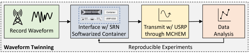
Figure 1. Waveform twinning on Colosseum.

3. Coexistence of Cellular and Radar Technologies in CBRS Band

In this section, we consider the use case of 4G/5G RANs transmitting in the CBRS band that needs to vacate said bandwidth because of an incoming radar transmission. CBRS regulations allow commercial broadband access to the RF spectrum ranging from $3.55$ GHz to $3.7$ GHz, as depicted in the Code of Federal Regulations (CFR) (of the Federal Register, United States). This spectrum is shared with various incumbents, including the U.S. military, which operates radar systems in this frequency range, e.g., shipborne radars along the U.S. coasts. According to the regulations, dynamic access to the spectrum is permitted as long as the network is able to detect the presence of the radar and activates interference mitigation measures when necessary (Caromi et al., 2018). As it will be described in Section 4, BSs leverage AI/ML agents —that can run as dApps— to perform inference on the received IQ samples and detect incoming radar transmissions, which will be described in Section 3.1. Once detected, BSs can either move to an unused bandwidth, if any, or terminate any ongoing communication to give priority to the radar. To effectively study this use case in the Colosseum wireless network emulator, we developed an RF propagation environment—located in the Waikiki Beach in Honolulu, Hawaii, described in Section 3.2—in which a coastline BS working in the CBRS bandwidth needs to vacate said bandwidth due to the start of radar transmissions from a boat moving in the North Pacific Ocean.

3.1. Radar Characterization

Radar systems leverage reflections of RF electromagnetic signals from a target to infer information on such target (Mahafza, 2017). Typical information may include detection, tracking, localization, recognition, and composition of the target, which may include aircraft, ships, spacecraft, vehicles, astronomical bodies, animals, and weather phenomena. Even though radar’s primary uses were mainly related to military applications, nowadays this technology is commonly used in other areas, such as weather forecasting, and automotive applications.

In this work, we leverage a weather radar that combines techniques typical of continuous-wave radars, e.g., pulse-timing to compute the distance of the target, and of pulse radars, like the Doppler effect of the returned signal to establish the velocity of the moving target (Doviak and Zrnić, 2006). Note that similar considerations can be applied to any other radar or waveform type, and the radar signal considered in this work is a use-case study (without loss of generality) to showcase Colosseum capabilities. Our radar operates in the S-Band, typically located within the $[3.0,3.8]$ GHz frequency range. The signal has been synthetically generated as a collection of IQ samples and timestamps, with a sampling rate of $6$ MS/s and 106657 sampling points for a total duration of $17.8$ ms. Figure 2 shows some characterization of the radar signal. Figure 2(a) depicts the Power Spectral Density (PSD) of the radar. Figure 2(b) displays the constellation diagram of the transmitted signal. We notice that the signal lies only in the first quadrant of the IQ-plane, which is typical of some radars.

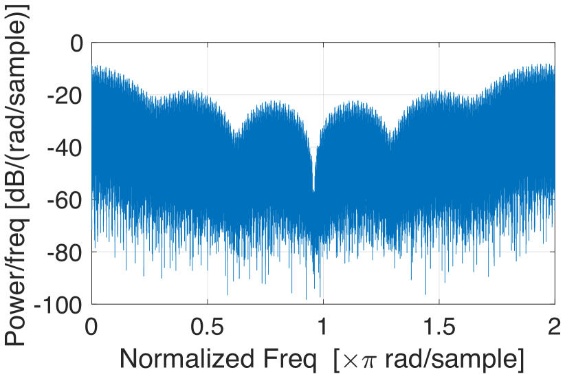
(a) Radar PSD

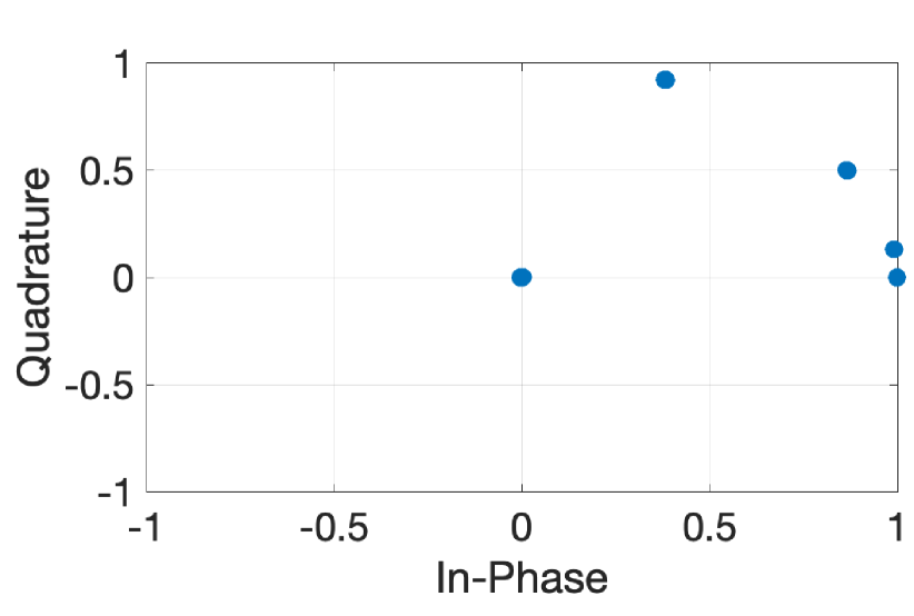
(b) Radar constellation

Figure 2. Radar characterization with PSD and constellation plots.

Figure 3 shows the various operations that we developed to integrate an arbitrary waveform (radar in this case) into the Colosseum environment.

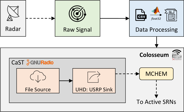
Figure 3. Block diagram of the operations needed to integrate the radar signal in Colosseum.

In the first step, the radar signal is generated either through a hardware device or in a synthetic manner. The output of this step is a raw signal formed of IQ samples for given time instances, which in our case is stored in a .csv file. The raw data is then processed to convert it into a format that can be interpreted by Colosseum. We use MATLAB to read the .csv raw signal and generate a .iq file with the array of IQ values sequentially saved in a float32 format. Finally, the newly created .iq file is transmitted in the Colosseum environment by leveraging the open-source CaST framework, which is based on GNU Radio (Villa et al., 2023; GNU Radio Project, 2023). For the purpose of this work, CaST has been modified to include a File Source block that allows us to load the .iq file on the Colosseum system. The signal is then passed through an UHD: USRP Sink block, which connects to the USRP SDR in Colosseum, and transmits the signal over MCHEM to the other SRNs.

Figure 4 shows the radar signal transmitted on the Colosseum wireless network emulator through CaST and received by another SRN.

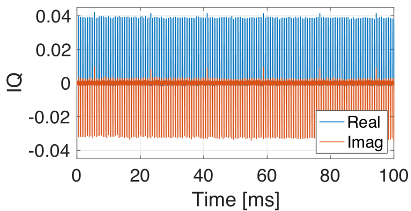
(a) Received radar waveform

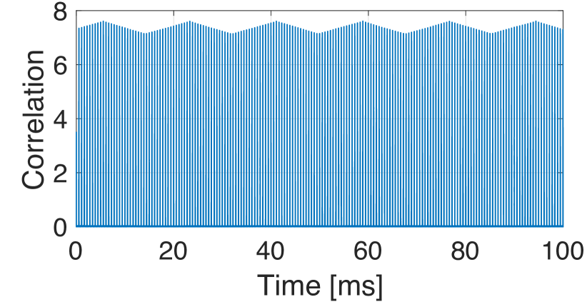
(b) Radar correlation

Figure 4. Results of a radar transmission through CaST.

Figure 4(a) displays real and imaginary parts of the raw radar waveform at the receiver node, while Figure 4(b) the correlation between the original radar signal and the received waveform. We notice that the correlation values are clearly visible, meaning that the radar signal is correctly transmitted and detected at the receiver side. We also notice a periodic jigsaw trend in the correlation results. This behavior is due to the large length of the transmitted radar IQ sequence (106657 complex points). Upon performing the correlation operation, the length of the sequence causes peaks at the beginning of the sequence, as well as valleys because of leftover samples from the correlation.

3.2. Colosseum Waikiki Beach Scenario

To validate our use case on Colosseum, we created a novel RF scenario that emulates the propagation environment of Waikiki Beach in Honolulu, Hawaii. This scenario involves a BS—whose location was taken from the OpenCelliD database (Unwired Labs, 2023) of real-world cellular deployments—that serves 6 UEs, and a radar-equipped ship that moves in the North Pacific Ocean. This scenario was created with the CaST toolchain (Villa et al., 2023) following the steps of Figure 5.

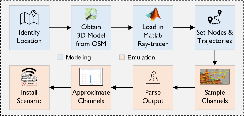
Figure 5. CaST scenario creation toolchain blocks diagram. Figure adapted from (Villa et al., 2023).

In the first step, we identify the scenario location. Since we are considering a ship node for the radar, we choose the coastal area of Waikiki Beach in Honolulu, Hawaii. Next, we obtain the 3D model of the selected location through the Open Street Map (OSM) tool (OpenStreetMap Foundation, 2023). We generate an .osm file of a rectangular area of about $700\times 800\>\mathrm{m}^{2}$, which includes Waikiki Beach, nearby buildings, and skyscrapers, as well as a portion of the ocean. We then load the 3D model into the MATLAB ray-tracer, and define the nodes of our scenario (shown in Figure 6) as well as their trajectories.

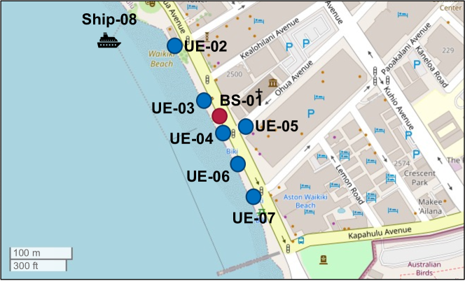
Figure 6. Location of the nodes in the Waikiki Beach scenario.

Our nodes are as follows.

• One cellular BS (red circle in Figure 6), whose antennas are located at $3$ m from the ground.

• Six static UEs (blue circles in Figure 6) uniformly distributed in the surroundings of the BS. UEs are located at $1$ m from the ground level to emulate hand-held devices.

• One ship (shown in black in Figure 6) equipped with a radar, whose antennas are located at a height of $3$ m. The ship moves following a North-South linear trajectory along Waikiki beach at a constant speed of $20$ knots ($\sim\!\!10$ m/s). This speed was derived as the average between the speed typical of civilian container ships—which travel at around $10$ knots ($\sim\!\!5$ m/s)—and that of aircraft carriers—which reach speeds of around $30$ knots ($\sim\!\!15$ m/s) (Taylor, 2013).

Table 1 summarizes the wireless parameters defined for the designed Colosseum RF emulation scenario.

Table 1. Parameters of the Waikiki Beach scenario.

Parameter	Value
Signal bandwidth	$20$ MHz
Transmit power (BS and ship)	$30$ dBm
Transmit power (UEs)	$20$ dBm
Antenna height (BS and ship)	$3$ m
Antenna height (UEs)	$1$ m
Building material	Concrete
Max number of reflections	$3$
Sampling time	$1$ second
Ship speed	$10$ m/s
Emulation area	$700x800\>\mathrm{m}^{2}$

Figure 7 shows the layout of the scenario loaded in the MATLAB ray-tracer. We notice the 3D model of the environment (white building blocks in the figure), together with the radio node locations (red icons), and the trajectory of the ship (green dots). In this step, we perform ray-tracing to characterize the environment of interest and derive the channel taps among each pair of the nodes of our scenario.

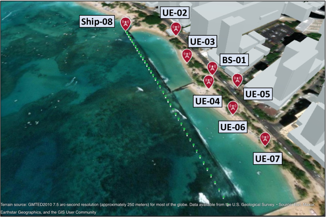
Figure 7. Layout of the scenario loaded in the MATLAB ray-tracer and visualized with Site Viewer.

After these operations are completed, the next step involves approximating the channel taps returned by the ray-tracer. This step is required to install the scenario in Colosseum, since MCHEM supports a maximum of 4 non-zero channel taps, with a maximum delay spread of $5.12\>\mu\mathrm{s}$. This is performed through a k-mean clustering algorithm that we previously developed (Tehrani Moayyed et al., 2021). The heat map of the path loss among each pair of nodes after this channel approximation step is depicted in Figure 8. (The ship node is considered to be in the top position at the beginning of the scenario.) As expected, closer nodes experience lower path loss values.

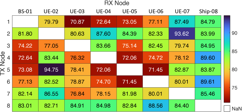
Figure 8. Heat map of the path loss among the nodes of the Waikiki scenario in Figure 7. The mobile ship node is considered in its starting position on the top.

As a final step, the channel taps are converted in FPGA-readable format, and the scenario is installed in Colosseum. Generating the channel taps with the ray-tracing software, and approximating them to the 4 non-zero taps required around $7$ hours by using a 2021 MacBook Pro M1 with 10 cores and $16$ GB of RAM. Installing the scenario on the Colosseum system required around $50$ minutes by leveraging a virtual machine hosted on a Dell PowerEdge M630 Server with 24 CPU cores and $96$ GB of RAM.

4. Intelligent Radar Detection

The BS leverages an AI model to detect radar signals during or before cellular communications. This section explains how we collect and pre-process the data before feeding it into our model, as well as the structure of the model itself.

4.1. Data Collection

By using the scenario of Section 3.2, radar and cellular signals are transmitted in different combinations and varying reception gain. Specifically, we collect IQ samples when only the radar is present, only the cellular signal is present, both are present, and neither is present (empty channel). These combinations encompass all the possible real scenarios that the intelligent radar detector might come across.

We pre-process these recordings by first breaking them into smaller samples of 1024 IQs, as this is the input size to the ML agent. This input size was chosen as we have found it to be the smallest size that still offers high classification performance. We then convert each sample to its frequency domain representation. Finally, we offer a binary label to each sample: 1 if radar exists in the sample, and 0 otherwise. In this way, the model groups empty channels and un-interfered cellular transmissions as 0 and therefore be free to communicate in the given band.

4.2. Model Design and Training

We utilize an altered and lightweight CNN for the radar detection. Specifically, we use a smaller version of VGG16 (Simonyan and Zisserman, 2014). We chose this structure as it is commonly used in wireless applications and can adequately show the capabilities of our framework.

Figure 9. CNN model used to train the radar detector.

The model architecture can be seen in Figure 9. For the first two convolutional blocks, we append a Non-local Block (NLB). These blocks help the CNN achieve self-attention and focus on spatially distant information. More on these blocks can be read in (Wang et al., 2018). This is a desirable trait as it can help identify long-range dependencies that may be present in the wireless signal rather than only focusing on adjacent IQs. The model takes as input IQs in the shape of $(batch\_size,1024,2)$ where the last dimension is the real and complex part of the IQ separated into two distinct channels.

5. Performance Evaluation

In this section, we present results on the effect of a radar signal on a cellular network deployed on the Colosseum wireless network emulator by showing: (i) the performance and accuracy of the ML intelligent detector model; and (ii) the Key Performance Indicators (KPIs), e.g., throughput, Channel Quality Information (CQI), and computation time of real-time experiments with and without radar transmissions and the intelligent detector.

5.1. Intelligent Detector Results

We test our radar detector on data withheld during training and observe an accuracy of 88%, a precision of 94%, and a recall of 79%. This tells us that our model is not susceptible to false positives (misclassifying empty channels or cellular signals as radar), but is susceptible to false negatives (misclassifying radar as an empty channel or a cellular signal).

To delve deeper into these results, we plot the accuracy as a function of SNR in Figure 10(a). For this plot, we keep the cellular nodes static in the scenario and only vary the radar gain. Here we can see that through varying SNRs we have very high and consistent performance in detecting radar signals, above 90%. However, when we add cellular signals into the channel, this makes the detection of radar more difficult, as can be seen in Figure 10(b), where we plot accuracy as a function of SINR. The cellular signal is considered as interference in this plot. Indeed, with high cellular signal gain and low radar gain, we see that our classification accuracy decreases to about 75%.

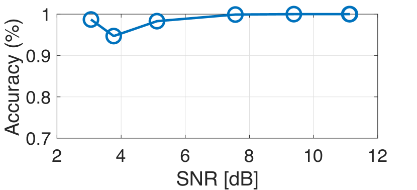
(a) SNR accuracy

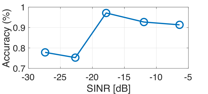
(b) SINR accuracy

Figure 10. CNN radar detection accuracy with varying SNR of the radar signal, and varying SINR where the cellular signal is considered to be interference.

5.2. Experimental Results

To properly study the network performance with and without the presence of radar transmissions, we leverage Colosseum and the newly created scenario described in Section 3.2 to deploy a cellular network and run traffic analysis. The parameters of the experiments are summarized

Table 2. Parameters of the experiments.

Parameter	Value
Center frequency	$3.6$ GHz
Signal bandwidth (radar)	$20$ MHz
Signal bandwidth (cellular)	$10$ MHz
Number of BSs	1
Number of UEs	6
USRP BS gains (Tx and Rx)	$[10,30]$ dB
USRP UE gains (Tx and Rx)	$20$ dB
USRP radar Tx gain	$20$ dB
Scenario Duration	$40$ s
Traffic type	UDP Downlink
Traffic rate	$10$ Mbps
Scheduling policy	Round-robin

in Table 2. The center frequency is set to $3.6$ GHz in the newly opened CBRS band, which is also used by S-Band-type radars. It is worth noticing that, even though characterized at $3.6$ GHz, the scenario has been installed in Colosseum at a center frequency of $1$ GHz, at which MCHEM is optimized to work. The scenario duration is set to $40$ s, which is the time needed by the ship to travel the planned $400$ m trajectory at the constant speed of $10$ m/s. Then, the scenario repeats cyclically from the beginning indefinitely.

We leverage the open-source SCOPE framework to deploy a twinned srsRAN protocol stack with one BS and six UEs (Bonati et al., 2021a; Gomez-Miguelez et al., 2016). Additionally, the radar signal is transmitted through the use of the CaST transmit node (Villa et al., 2022), which has been modified to support custom radio waveforms. In the following subsections, we show the results for three main cellular network use cases: (i) no radar transmission; (ii) with radar signal interference; and (iii) with radar and intelligent detector. In all experiments, a User Datagram Protocol (UDP) downlink traffic of $10$ Mbps among BS and UEs is generated through iPerf, a tool to benchmark the performance of Internet Protocol (IP) networks.

5.2.1. No Radar

The performance of the cellular network, in terms of downlink throughput and CQI, without radar transmissions is shown in Figure 11, from second $0$ to $150$. The gains of the BS USRP are set to $25$ dB.

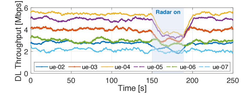
(a) Downlink throughput

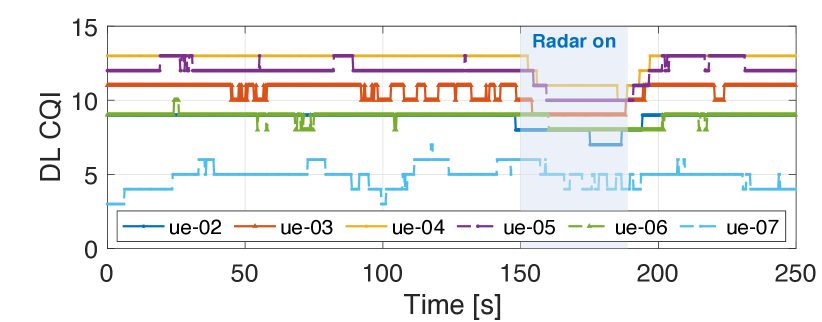
(b) Downlink CQI

Figure 11. Moving average of cellular network downlink throughput and CQI. A radar transmission is ongoing from second 150 to second 190, highlighted with a blue shade.

As expected, the throughput, shown in Figure 11(a), decreases with the increase of the distance between UEs and BS. The best performance is achieved by UE-04, with values between $5.22$ and $5.71$ Mbps, while the other UEs experience a performance between $1.82$ and $5.25$ Mbps. The worst throughput is achieved by UE-07 due to its large distance from the BS, environment conditions, and interference with the other nodes. The CQI, shown in Figure 11(b), follows a similar trend. Best values are reported by UE-04, with a stable CQI of $13$. The other UEs show CQI values between $2$ and $13$, with UE-07 reporting the lowest CQI values (between $2$ and $7$).

5.2.2. Radar

The impact of radar transmissions on the cellular performance is shown in Figure 11, from second $150$ to $190$. As expected, we notice a drop in the throughput (Figure 11(a)) and CQI values reported by the UEs (Figure 11(b)). This is more visible for the nodes closer to the BS, e.g., UE-03, UE-04, and UE-05, since they get more affected by the radar transmission. When the radar stops transmitting, i.e., at around second $190$, the performance of the UEs goes back to the initial values, i.e., to the values in the $[0,150]$ s window.

5.2.3. Intelligent Radar Detection

In this last use case, we evaluate the effectiveness of our intelligent detector in understanding the presence of the radar signal, as shown in Figure 12.

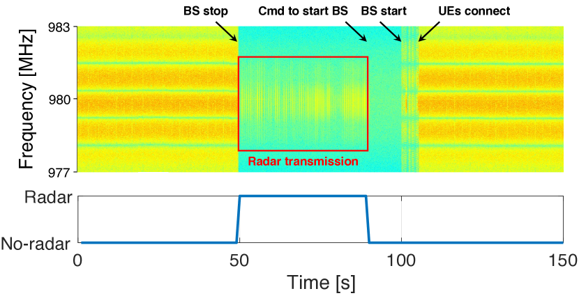
Figure 12. (top) Downlink cellular spectrogram; (bottom) radar detection system. The BS is shut down when a radar transmission is detected and resumes normal operations after no radar is detected.

The top portion of the figure shows the downlink cellular spectrogram centered at $980$ MHz (i.e., the downlink center frequency we use for srsRAN in Colosseum) with a $6$ MHz span; the bottom one displays the results of the radar detection system. At the beginning of the experiment—from second $0$ to second $50$—the BS is serving the UEs through UDP downlink traffic (Figure 12, top), as we notice from the orange and yellow stripes. Then, at second $50$, a radar transmission is detected by the intelligent detector (Figure 12, bottom) described in Section 4, and the BS is shut down accordingly. After the radar transmission ends, i.e., at second $90$, the BS receives the command to power back on and, after around $10$ seconds, it resumes its operations (second $100$). Finally, at second $110$, the UEs reconnect to the BS, and the downlink transmissions are restarted. Overall, this demonstrates the effectiveness of our intelligent detector in identifying radar signals and vacating the cellular bandwidth. Note that even if we have not tested our ML agent with different radar signal types, changes in the radar waveform that impact its frequency domain representation might require a re-training of the model to achieve similar performance.

Figure 13 shows the required computation time for the classification, performed on CPU, with different batch sizes in a Colosseum SRN.

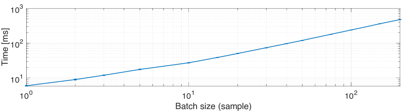
Figure 13. Computation time required for a radar classification, with different batch sizes, run on CPU on a Colosseum SRN with 48-cores Intel Xeon processor and 126 GB of RAM.

We notice that values grow linearly with the batch size, e.g., $6$ ms for a batch size of 1 sample, $27.4$ ms for 10, $239$ ms for 100. This can be traced back to the fact that these operations run on CPU, so there is not much parallelization of the processes as it would be in a GPU. However, even in the case of a batch size of 100 samples, the maximum time of $60$ seconds required for the detection of commercial transmissions in the CBRS band is satisfied (Goldreich, 2016). To avoid false positives and false negatives, we leverage a voting system of 100 samples, in which the signal to shut down the BS is sent only when more than $50$% of the outputs are detecting a radar. Moreover, we use a batch size of 10 samples, which gives us a good tradeoff between computation time and granularity of the output samples needed for the voting system. In these conditions, our intelligent detector is able to detect an incumbent radar transmission and vacate the cellular bandwidth within $137$ ms—which is the average time for the ML model to generate 50 new outputs with a batch size of 10 samples—and with an accuracy of $88$%.

6. Conclusions

In this work, we developed a framework for high-fidelity emulation-based spectrum-sharing scenarios with cellular and radar nodes implemented as a digital twin system on the Colosseum wireless network emulator. First, we twinned the radar waveform on Colosseum, then we collected IQ samples of radar and cellular communications in different conditions. Finally, we trained a CNN network —that can run as a dApp— to detect the presence of the radar signal and halt the cellular network to eliminate the undesired interference on the incumbent radar communications. Our experimental results show that our detector obtains an average accuracy of 88% (above 90% when SNR and SINR are greater than $0$ dB and $-20$ dB respectively), and requires an average time of $137$ ms to detect ongoing radar transmissions.

- (1)
- Baldesi et al. (2022) L. Baldesi, F. Restuccia, and T. Melodia. 2022. ChARM: NextG Spectrum Sharing Through Data-Driven Real-Time O-RAN Dynamic Control. In Proceedings of IEEE INFOCOM.
- Bonati et al. (2021a) L. Bonati, S. D’Oro, S. Basagni, and T. Melodia. 2021a. SCOPE: An Open and Softwarized Prototyping Platform for NextG Systems. In Proceedings of ACM MobiSys.
- Bonati et al. (2021b) L. Bonati, P. Johari, M. Polese, S. D’Oro, S. Mohanti, M. Tehrani-Moayyed, D. Villa, S. Shrivastava, C. Tassie, K. Yoder, A. Bagga, P. Patel, V. Petkov, M. Seltzer, F. Restuccia, M. Gosain, K. R. Chowdhury, S. Basagni, and T. Melodia. 2021b. Colosseum: Large-Scale Wireless Experimentation Through Hardware-in-the-Loop Network Emulation. In Proceedings of IEEE DySPAN.
- Caromi et al. (2018) R. Caromi, M. Souryal, and WB Yang. 2018. Detection of Incumbent Radar in the 3.5 GHz CBRS Band. In Proceedings of IEEE GlobalSIP. 241–245.
- D’Oro et al. (2022) S. D’Oro, M. Polese, L. Bonati, H. Cheng, and T. Melodia. 2022. dApps: Distributed Applications for Real-Time Inference and Control in O-RAN. IEEE Communications Magazine 60, 11 (November 2022), 52–58.
- Doviak and Zrnić (2006) R. J. Doviak and D. Zrnić. 2006. Doppler Radar and Weather Observations. Courier Corporation.
- Gao et al. (2019) J. Gao, X. Yi, C. Zhong, X. Chen, and Z. Zhang. 2019. Deep Learning for Spectrum Sensing. IEEE Wireless Communications Letters 8, 6 (September 2019), 1727–1730.
- GNU Radio Project (2023) GNU Radio Project. Accessed June 2023. GNU Radio. https://www.gnuradio.org
- Goldreich (2016) O. Goldreich. 2016. Requirements for Commercial Operation in the U.S. 3550-3700 MHz Citizens Broadband Radio Service Band. In Wireless Innovation Forum.
- Gomez-Miguelez et al. (2016) I. Gomez-Miguelez, A. Garcia-Saavedra, P.D. Sutton, P. Serrano, C. Cano, and D.J. Leith. 2016. srsLTE: An Open-source Platform for LTE Evolution and Experimentation. In Proceedings of ACM WiNTECH. New York City, NY, USA.
- Luo et al. (2022) G. Luo, Q. Yuan, J. Li, S. Wang, and F. Yang. 2022. Artificial Intelligence Powered Mobile Networks: From Cognition to Decision. IEEE Network 36, 3 (July 2022), 136–144.
- Mahafza (2017) B. R. Mahafza. 2017. Introduction to Radar Analysis. CRC press.
- of the Federal Register (United States) Office of the Federal Register (United States). 2016. Citizens Broadband Radio Service. Vol. 96. Code of Federal Regulations.
- OpenStreetMap Foundation (2023) OpenStreetMap Foundation. Accessed June 2023. OpenStreetMap. https://www.openstreetmap.org.
- Platforms for Advanced Wireless Research (2023) Platforms for Advanced Wireless Research. Accessed June 2023. https://www.advancedwireless.org.
- Polese et al. (2023) M. Polese, L. Bonati, S. D’Oro, S. Basagni, and T. Melodia. 2023. Understanding O-RAN: Architecture, Interfaces, Algorithms, Security, and Research Challenges. IEEE Communications Surveys & Tutorials 25, 2 (January 2023), 1376–1411.
- Simonyan and Zisserman (2014) K. Simonyan and A. Zisserman. 2014. Very Deep Convolutional Networks for Large-scale Image Recognition. arXiv preprint arXiv:1409.1556 [cs.CV] (September 2014).
- Taylor (2013) D. W. Taylor. 2013. The Speed and Power of Ships. Books on Demand.
- Tehrani Moayyed et al. (2021) M. Tehrani Moayyed, L. Bonati, P. Johari, T. Melodia, and S. Basagni. 2021. Creating RF Scenarios for Large-scale, Real-time Wireless Channel Emulators. In Proceedings of IEEE MedComNet. Virtual Conference.
- Unwired Labs (2023) Unwired Labs. Accessed June 2023. OpenCelliD. https://opencellid.org.
- Villa et al. (2022) D. Villa, M. Tehrani-Moayyed, P. Johari, S. Basagni, and T. Melodia. 2022. CaST: A Toolchain for Creating and Characterizing Realistic Wireless Network Emulation Scenarios. In Proceedings of ACM WiNTECH. Sydney, Australia.
- Villa et al. (2023) D. Villa, M. Tehrani-Moayyed, C. P. Robinson, L. Bonati, P. Johari, M. Polese, S. Basagni, and T. Melodia. 2023. Colosseum as a Digital Twin: Bridging Real-World Experimentation and Wireless Network Emulation. arXiv:2303.17063 [cs.NI] (March 2023), 1–15.
- Wang et al. (2018) X. Wang, R. Girshick, A. Gupta, and K. He. 2018. Non-local Neural Networks. In Proceedings of the IEEE/CVF Conference on Computer Vision and Pattern Recognition. Salt Lake City, UT, USA.
- Wang et al. (2019) Y. Wang, M. Liu, J. Yang, and G. Gui. 2019. Data-Driven Deep Learning for Automatic Modulation Recognition in Cognitive Radios. IEEE Transactions on Vehicular Technology 68, 4 (February 2019), 4074–4077.
- Zheng et al. (2020) S. Zheng, S. Chen, P. Qi, H. Zhou, and X. Yang. 2020. Spectrum Sensing Based on Deep Learning Classification for Cognitive Radios. China Communications 17, 2 (February 2020), 138–148.