An experimental realisation of steady spanwise forcing for turbulent drag reduction

Abstract

We present an experimental realisation of spatial spanwise forcing in a turbulent boundary layer flow, aimed at reducing the frictional drag. The forcing is achieved by a series of spanwise running belts, running in alternating spanwise direction, thereby generating a steady spatial square-wave forcing. Stereoscopic particle image velocimetry is used to investigate the impact of actuation on the flow in terms of turbulence statistics, performance characteristics, and spanwise velocity profiles, for a waveform of $\lambda_{x}^{+}=401$. An extension of the classical spatial Stokes layer theory is proposed based on the linear superposition of Fourier modes to describe the non-sinusoidal boundary condition. The experimentally obtained spanwise profiles show good agreement with the extended theoretical model. In line with reported numerical studies, we confirm that a significant flow control effect can be realised with this type of forcing. The results reveal a maximum drag reduction of 26% and a maximum net power savings of 8%. In view of the limited spatial extent of the actuation surface in the current setup, the drag reduction is expected to increase further as a result of its streamwise transient. The second-order turbulence statistics are attenuated up to a wall-normal height of $y^{+}\approx 100$, with a maximum streamwise stress reduction of 44% and a reduction of integral turbulence kinetic energy production of 39%.

1 Introduction

Turbulent drag reduction is a crucial research area in fluid dynamics, as reducing drag can lead to substantial energy savings and emission reductions in a variety of industrial and transportation applications. Spanwise forcing of the turbulent boundary layer through transverse wall motion has shown significant potential for turbulent drag reduction (DR), with reported DR values reaching over 40% (Ricco et al., 2021). To account for the energy expenditure of the forcing, the net power saving (NPS) is defined as the difference between the DR and the idealised power input to drive the spanwise velocity profile.

Early work on spanwise forcing focused on oscillating wall (OW) motion, where a wall section is subjected to a temporal oscillation. The strategy was first studied using direct numerical simulations (DNS) by Jung et al. (1992); a DR of 40% was found at a spanwise velocity amplitude of $A^{+}=12$ and an optimum period of $T^{+}=100$. The characteristic parameters are commonly scaled in viscous units, with the kinematic viscosity $\nu$ and the friction velocity $u_{\tau}\equiv\sqrt{\tau_{w}/\rho}$; $\tau_{w}$ and $\rho$ are the wall-shear stress and fluid density. Furthermore, we distinguish two scaling approaches, using either the reference $u_{\tau 0}$ from the non-actuated case or the actual $u_{\tau}$ of the drag-reduced flow case; these are denoted by the superscript ‘+’ and ‘*’, respectively. Laadhari et al. (1994) conducted experiments which corroborated the results of Jung et al. (1992). They reported a DR of 36% using the same actuation parameters. Following their work, OW forcing has been extensively researched over several decades, in both experimental and numerical studies (Ricco et al., 2021). Another form of spanwise forcing was introduced by Quadrio et al. (2009), by imposing a spatio-temporal oscillation, which results in a travelling wave (TW) boundary condition. A maximum DR of 48% was observed at $A^{+}=12$. Inspired by their work, several experimental realisations of TW forcing have been made. Examples are the deformable kagome lattice of Bird et al. (2018), and a more recent contribution of Marusic et al. (2021), who employed a series of synchronised spanwise oscillatory elements. The mechanism responsible for the DR lies in part in the oscillatory nature of the resulting spanwise velocity profile. This profile predominantly resides within the viscous region of the boundary layer, thereby showing a close match to the laminar solution of the second Stokes problem, or temporal Stokes layer (TSL), in the case of OW forcing. In spatio-temporal form, the solution is described by the generalised Stokes layer (GSL), as introduced by Quadrio & Ricco (2011). Regarding the working mechanism, Ricco (2004) presents evidence that the Stokes profile breaks up the interaction between the near-wall streaks and the quasi-streamwise vortices by laterally displacing the two features. Their disrupted spatial coherence decreases the strength of the near-wall cycle resulting in a drag-reduced state.

A third actuation scheme is a pure spatial forcing, which has been the focus in a small number of numerical studies (e.g Viotti et al., 2009; Yakeno et al., 2009; Skote, 2013). Forcing is imposed in this case as a steady wall velocity in the form of a standing wave (SW):

$$W_{w}(x)=A\sin\left(\frac{2\pi}{\lambda_{x}}x\right),$$ (1)

in which $A$ is the spanwise velocity amplitude and $\lambda_{x}$ the streamwise wavelength of actuation. In this work, the $x$, $y$, and $z$ coordinates denote the streamwise, wall-normal, and spanwise directions, respectively, which correspond to instantaneous velocity components $u$, $v$, and $w$. Applying Reynolds decomposition, an overbar and prime indicate the mean and fluctuating component, respectively. The oscillatory spanwise forcing of the flow is in this concept achieved convectively, as the flow travels over the regions of alternating forcing direction. SW forcing was first introduced and numerically studied by Viotti et al. (2009), and an optimum DR of 45% was found around $\lambda_{x}^{+}=1,000-1,250$ at $A^{+}=12$. Their results were compared to OW simulations of Quadrio & Ricco (2004), under a convective transformation. The same trends could be observed; quantitatively, the DR potential was found to be about 20-30% higher. Under SW forcing, the GSL reduces to the spatial Stokes layer (SSL). The work of Auteri et al. (2010) realised TW forcing in their pipe flow setup, where the wave was generated by means of multiple azimuthally rotating pipe segments. Although SW forcing was not the primary focus of their studies, under steady conditions, spatial forcing was obtained. Besides this study, no experimental realisations of SW forcing have been reported.

To address the sparse attention devoted to SW forcing so far, especially experimentally, we present a proof of concept for an experimental realisation of such forcing in an external boundary layer flow. The setup consists of an array of spanwise running belts, so as to generate a steady spatial square-wave wall boundary condition. A theoretical model for the SSL for an arbitrary waveform is proposed, by using linear superposition of Fourier modes that describe the non-sinusoidal boundary condition. The resultant modified SSL is compared to the experimentally obtained spanwise profiles. The flow modulation effects and its performance characteristics are assessed using stereoscopic particle image velocimetry (SPIV).

2 Experimental methodology

Experiments were performed in the M-tunnel of the Delft University of Technology at a freestream velocity of $U_{\infty}\approx 6.7$ m/s and a freestream turbulence intensity of the order of 0.7%. The open-return tunnel has a test section with a cross-section of 0.4 m × 0.4 m. A clean turbulent boundary layer was generated on a horizontally oriented flat plate with an elliptical leading edge and tripped using carborundum roughness (24 grit), achieving a development length of 3 m. The experimental setup was placed in an open-jet configuration, behind and flush with the test section. A temperature sensor and Pitot-static tube were used to monitor ambient conditions and freestream velocity. In view of the limited field of view of the SPIV experiment, the reference boundary layer under non-actuated conditions was characterised over its full height using hot-wire anemometry. The hot-wire probe was positioned 3 mm downstream of the actuation surface. The characteristics for the current experimental conditions are $\delta=67$ mm ($\delta$ denotes the boundary layer thickness), $u_{\tau 0}=0.27$ m/s, yielding $\Rey_{\tau}=1230$, where the friction Reynolds number is defined as $\Rey_{\tau}\equiv\delta u_{\tau 0}/\nu$.

2.1 Steady spanwise excitation setup

The experimental setup, referred to as the steady spanwise excitation setup (SSES), was designed to realise SW forcing experimentally in an external boundary layer flow. Four streamwise-spaced, spanwise running belts, run in alternating direction so as to generate a spatial square actuation waveform. The simplification of using a square waveform instead of a sinusoidal waveform is justified by the studies of Cimarelli et al. (2013) and Mishra & Skote (2015), who showed that substantial DR and NPS could be obtained using non-sinusoidal forcing. A schematic representation of the setup and its constituting components are presented in figure 1.

Figure 1: Schematic representation of the SSES mechanism, and its placement with respect to the wind tunnel exit. Arrows on the belts indicate their respective rotation directions.

The SSES has four 9 mm wide neoprene belts, extending over a spanwise extent of 256 mm. The streamwise separation of 2 mm between the belts is kept to a minimum considering the mechanical feasibility of the design. We define the start of the waveform, and the origin of the coordinate system, at 1 mm (i.e. half the streamwise separation) upstream of the first belt. The belts are embedded in an aluminium surface plate so as to run flush with the wall. In addition, the belts are guided by a PTFE strip to constrain the belts to the surface grooves. The grooves are precisely machined to strict tolerances, with a maximum gap and step size of 50 µm. The belts are driven by a non-slip pulley system, which allows for individually controlling the rotation direction of the belts. The SSES is powered by two iHSV60 integrated AC servo motors that drive the belts in positive and negative spanwise direction. The motors have an adjustable feedback control loop for a fixed belt velocity output, with a maximum spanwise velocity of 6 m/s. An advantage of such a setup is the independent control over $A$ and $\lambda_{x}$, which are usually coupled in OW and TW forcing which employ oscillating elements with a fixed displacement amplitude.

2.2 Stereoscopic particle image velocimetry

SPIV was used to obtain the three velocity components in the streamwise-wall-normal ($x-y$) plane. Each measurement consists of 1000 uncorrelated velocity fields, obtained at an acquisition frequency of 10 Hz. Two digital LaVision sCMOS cameras (2,560 × 2,160 pixels, 6.5 µm pixel size) were placed on either side of the laser sheet in back-scatter configuration. The field of view (FOV) was centred on the middle two belts of the SSES, spanning 24 mm × 14.5 mm in the $x$ and $y$ direction, respectively. The corresponding spatial resolution is 113 pixels/mm. Imaging was performed using Nikkor AF-S 200 mm lenses, with Kenko Teleplus PRO 300 $2\times$ teleconverters, at an aperture of f/11. The cameras were oriented at $\pm 30^{\circ}$ with respect to the laser sheet normal. Scheimpflug adapters were used to ensure uniform focus across the FOV. Illumination was provided by a Quantel Evergreen 200 laser (double-pulsed ND:Yag, 532 nm), with a 100 mJ/pulse power setting. A combination of cylindrical and spherical lenses was used to create a laser sheet with an approximate thickness of 1 mm. Seeding was injected at the wind tunnel inlet by a SAFEX Fog 2010+ fog generator to create 1 µm tracer particles from a water-glycol mixture.

Stereo calibration was performed to transform the images to physical coordinates. Additionally, self-calibration was performed to reduce the calibration fit error to below 0.25 pixel. For each camera, the two velocity component fields were obtained using cross-correlation, with 16 × 16 pixels circular interrogation windows at 75% overlap. The resulting vector pitch was 0.035 mm or $0.64\nu/u_{\tau 0}$. The resultant velocity fields of the two cameras were combined to obtain the 2D3C velocity field by a least squares fitting approach. The average stereo reconstruction error was below 0.1 pixel. Wall-normal profiles of the turbulence statistics were obtained by ensemble averaging (denoted by $\langle\rangle$) in time and streamwise direction, spanning $0.5\leq x/\delta\leq 1.5$. This method allows us to assess the integral effect of actuation over one streamwise actuation wavelength. The uncertainty was quantified using the uncorrelated samples, i.e. every fourth element in the streamwise direction to account for the 75% overlap. The uncertainties for the non-actuated case, at $y^{+}=15$, are 0.069% and 0.36% for the mean streamwise velocity and streamwise Reynolds stress, respectively.

2.3 Boundary layer fitting and estimation of the drag reduction

The reference friction velocity $u_{\tau 0}$ was obtained from a fitting the streamwise velocity profile to the inner-layer profile of Chauhan et al. (2009) using a sequential quadratic programming iterative method. To constrain the fitting procedure in order to obtain consistent values, the log-layer parameters are kept constant, where standard values of $\kappa=0.384$ and $B=4.17$ have been used (Nagib & Chauhan, 2008). Under drag-reduced conditions, the procedure as outlined cannot be applied, due to the deviation from the canonical profile. To obtain the viscous scaling under drag-reduced conditions, the measured velocity data in the region of $3\leq y^{+}\leq 5.5$ (encompassing four data points) is fitted to the theoretical relation $u^{*}=y^{*}$. Note that although the fitting domain is obtained from the non-actuated case, the linear relation is still valid under drag-reduced flow conditions as the viscous length scale increases. The maximum standard error of $u_{\tau}$ was 0.78%. The DR is defined as the reduction in mean wall-shear stress, which can be expressed in terms of $u_{\tau}$ as:

$$\text{DR}=1-\frac{\tau_{w}}{\tau_{w0}}=1-\left(\frac{u_{\tau}}{u_{\tau 0}}\right)^{2}.$$ (2)

3 Laminar solution of the spatial Stokes layer for an arbitrary waveform

An extension of the laminar SSL model is required to allow for the representation of an arbitrary waveform of the spanwise wall velocity. The classical Stokes layer solution is derived from the $z$-momentum equation of the laminar boundary layer equations, under the assumption that the characteristic wall-normal length scale ($\delta_{x}$) is small compared to the outer-scale. Full details on the derivation can be found in Viotti et al. (2009). The solution corresponding to a harmonic waveform reads as follows:

$$w(x,y)=AC_{x}\Real\left[e^{\mathrm{i}k_{x}x}\Ai\left(-\frac{\mathrm{i}y}{\delta_{x}}e^{-\mathrm{i}4\upi/3}\right)\right],$$ (3)

with

$$\delta_{x}=\left(\frac{\nu}{k_{x}u_{y,0}}\right)^{1/3},$$ (4)

where $C_{x}=\Ai(0)^{-1}$ is a normalisation constant, $\mathrm{i}$ is the imaginary unit, $k_{x}$ is the streamwise wavenumber and $u_{y,0}$ is the slope of the streamwise velocity profile at the wall. We now adapt the SSL solution to account for an arbitrary waveform, following the approach taken by Cimarelli et al. (2013) for the TSL. The linear nature of the governing equation allows for a superposition of various harmonics to make up the desired waveform. In line with their approach, the waveform describing the wall motion is expressed in terms of a Fourier series:

$$W_{w}(x)=A\sum_{n=-\infty}^{+\infty}B_{n}e^{\mathrm{i}k_{x}nx},$$ (5)

where $B_{n}$ is the complex coefficient and $k_{x}n$ the wavenumber associated with the n^th Fourier mode. The corresponding penetration depth is defined as:

$$\delta_{x,n}=\left(\frac{\nu}{k_{x}nu_{y,0}}\right)^{1/3}=\delta_{x}n^{-1/3}.$$ (6)

Substituting this and superimposing the elementary solutions, the SSL for an arbitrary waveform is then found as follows:

$$w(x,y)=AC_{x}\sum_{n=-\infty}^{+\infty}\Real\left[B_{n}e^{ik_{x}nx}Ai\left(-\frac{iy}{\delta_{x}n^{-1/3}}e^{-i4\upi/3}\right)\right].$$ (7)

4 Experimental results and discussion

The experimental setup was used in a configuration where the belts move in alternating spanwise direction, resulting in the sequence of two square waveforms of $\lambda_{x}=22$ mm, and a viscous wavelength of$\lambda_{x}^{+}=401$. Six cases are discussed at varying spanwise amplitude from $A^{+}\approx 2$ to $12$.

4.1 Comparison to the modified spatial Stokes layer

To address how the experimentally realised forcing relates to the theoretical SSL, we compare the measured spanwise profiles to the model of the modified SSL derived in § 3. The periodic waveform, consisting of two 9 mm regions actuated at $\pm A$, is prescribed by ten single-sided Fourier coefficients. The 2 mm transition between belts is approximated by a linear increase from $-A$ to $A$ to prevent Gibbs phenomena. We investigate the case at $A^{+}=6.3$. The half-phase ($\lambda_{x}/2$) is used to normalise the streamwise location. Consequently, the same value after the decimal point indicates the same location on the half-phase. The experimental profiles are is subjected to streamwise averaging across the $x\pm 0.25$ mm range.

The spanwise profiles at three locations for each half-phase (i.e. belt) are presented in figure 2(a), where $\tilde{w}$ denotes the phase-wise component as a result of the forcing. We observe that the profiles resemble a clear Stokes-like layer, with a steep spanwise velocity gradient at the wall, followed by an overshoot around $y^{+}\approx 10$, after which it decays to zero at $y^{+}\approx 25$. The behaviour is consistent with the SSL model, subject to equation 1, at moderate wavelengths (Quadrio & Ricco, 2011; Viotti et al., 2009). Some small degree of asymmetry between the two half-phases can be observed. This may be attributed to a spatial transient of the SSL, which only sees actuation over one half-phase upstream of the FOV.

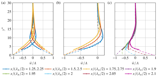
Figure 2: Spanwise velocity profiles at $\lambda_{x}^{+}=401$ and $A^{+}=6.3$, where the colour denotes the location on the half-phase. Experimental data plotted with solid lines, modified SSL displayed for the same colour indicated with a dashed-dotted line. (a) Profiles over the belts at three locations per half-phase, (b) a detailed view of the profiles over the first half-phase, (c) five linearly spaced profiles in the transition region between belts.

To make a comparison to the theoretical model for the modified SSL, the first half-phase is highlighted in more detail in figure 2(b). The experimental profiles match the model well, with an almost exact match in the region $y^{+}\leq 10$. The slope of the spanwise velocity profile is in line with the model and decreases when moving downstream over the belt. Hence, the model can be used to estimate the power input required to drive the spanwise flow, which is calculated from the integral spanwise wall shear stress (i.e. $\propto\left.(\mathrm{d}\tilde{w}/\mathrm{d}y)\right|_{y=0}$). We utilised the model to estimate the input power, followed by the calculation of NPS, further discussion on these outcomes is presented in § 4.2. Beyond $y^{+}=10$ it can be observed that the experimental data starts to divert from the theory. The overshoot of the experimental profile is larger in magnitude, present at higher wall-normal locations, and penetrates deeper into the boundary layer. These differences may be attributed to turbulent flow further away from the wall, in contrast to the laminar flow assumption of the SSL model.

The idealised model furthermore deviates from the practical realisation by linearly transitioning between half-phases, instead of the abrupt changes and the zero spanwise wall velocity in the transition region. To assess the effect of this choice, five linearly spaced profiles spanning $0.9\leq x/(\lambda_{x}/2)\leq 1.1$ in the transition region are studied, as depicted in figure 2(c). A good match between the model and the experiment can be observed, showing only slight deviations in the region $y^{+}\leq 5$. The penetration depth is defined as the wall-normal location where the phase-wise standard deviation of $\tilde{w}$ reduces to $Ae^{-1}$. The model and experimental values are $\delta_{s,mod}^{+}=5.0$ and $\delta_{s,exp}^{+}=4.8$, respectively. At first glance this result appears conflicting, since the experimental profile, specifically the overshoot, perpetrates deeper into the boundary layer. However, following the above definition, the penetration depth is confined to the viscous sublayer. In this region the model shows a slightly higher variance, explaining the small difference. Since there are only minor variations, we conclude that the current way of modelling can be applied without significantly altering the response of the Stokes profiles.

4.2 Mean velocity and performance characteristics

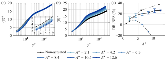
Figure 3: (a-b) Streamwise velocity profiles for the non-actuated case and cases with $\lambda_{x}^{+}=401$, (a) scaling with $u_{\tau 0}$, (b) scaling with $u_{\tau}$. (c) DR (solid) and NPS (dashed) vs $A^{+}$ compared to the DR of Viotti et al. (2009) for $\lambda_{x}^{+}=312$ (dotted), error bars indicate the 95% confidence interval of DR calculated using Student’s t-distribution.

The mean streamwise velocity profiles are shown in figure 3(a,b), in scaling with the reference and actual friction velocity, respectively. Scaling with $u_{\tau 0}$ reveals a reduction of mean velocity below $y^{+}\leq 15$, which is correlated with $A^{+}$. This reflects a reduction of the near-wall velocity gradient, indicative of a drag-reduced state. The behaviour is consistent with previous studies on spanwise forcing (Ricco & Wu, 2004; Gatti & Quadrio, 2016). To further emphasise this, scaling with $u_{\tau}$ is applied. The profiles now show similarity in the viscous sublayer with an upward shift $\Delta B$ of the logarithmic region under actuation, consistent with the reduction in skin friction. The profiles, specifically noticeable in figure 3(a), reveal an overshoot of the velocity profile in the region $20\leq y^{+}\leq 40$ compared to the non-actuated case. These results are consistent with the conceptual model of Choi (2002), which suggests that this modification of the streamwise velocity profile is due to an induced negative spanwise vorticity.

The performance characteristics are quantified in figure 3(c), where for reference the data of DR from the DNS of Viotti et al. (2009) is added, subject to equation 1 with $\lambda_{x}^{+}=312$ at $\Rey_{\tau}=200$. The DR increases monotonically at a decreasing rate with $A^{+}$, to a maximum value of 26%. Qualitatively this behaviour compares well to the DNS reference. In absolute terms, the DR is lower, especially at higher values of $A^{+}$. This is primarily attributed to the expected streamwise transient of DR from the onset of actuation. As shown by Ricco & Wu (2004), the DR rises to a maximum over a streamwise extent of $3\delta$, whereas our measurement domain extends over only $0.16\leq x/\delta\leq 0.50$. Secondly, a slight drop in performance is expected from the higher Reynolds number in the experimental conditions (Gatti & Quadrio, 2016). Lastly, the experimental realisation of the SW boundary condition may not perform to the same degree as the idealised conditions in the numerical studies. The NPS exhibits a maximum of 8% in the range of $A^{+}=2.1-4.2$, whereas Viotti et al. (2009) achieved an optimum of 23% at $A^{+}=6$. The maximum is followed by a sharp decline to large negative values (not depicted for clarity), reaching a minimum of -51% for $A^{+}=12.6$. This behaviour results from the balance between DR and input power ($\propto A^{+}$). We believe the difference in optimum is a consequence of the higher DR towards the lower $A^{+}$ values, and the higher power requirements for square-wave forcing.

4.3 Higher-order turbulence statistics

The higher-order turbulence statistics in terms of the variance profiles for the three velocity components, the Reynolds shear stress, and the turbulence kinetic energy (TKE) production are depicted in figure 4. Reference scaling with $u_{\tau 0}$ is applied to highlight the absolute changes with respect to the non-actuated case.

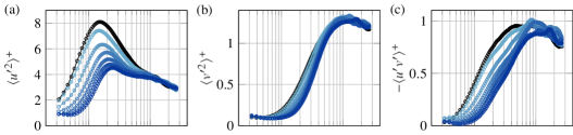
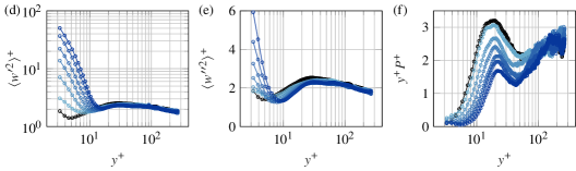
Figure 4: (a,b) Streamwise and wall-normal Reynolds stresses and (c) Reynolds shear stress. Spanwise stress is decomposed in (d) total spanwise stress and (e) the stochastic component. (f) Premultiplied production of turbulence kinetic energy. Legend is depicted in figure 3.

Assessing figure 4(a), we observe that upon actuation the streamwise stress is attenuated in the region up to $y^{+}\approx 100$, and that the near-wall peak is shifted to higher wall-normal positions. In line with the DR behaviour, the effect is correlated with $A^{+}$. The most significant reduction is found in the near-wall stress peak, which is centred around $y^{+}=15$ for the non-actuated case. The near-wall peak shows a $44\%$ reduction in magnitude for the maximum $A^{+}$. This response is consistent with earlier experimental observations of drag-reduced flow under spanwise forcing (Laadhari et al., 1994; Ricco & Wu, 2004). The stresses $\langle v^{\prime 2}\rangle^{+}$ and $-\langle u^{\prime}v^{\prime}\rangle^{+}$, in figure 4(b,c), reflect similar behaviour, where the profiles shift to higher wall-normal locations and attenuation is most significant close to the wall.

Under periodic forcing, the total spanwise stress is decomposed into a stochastic component and a phase-averaged component, according to $\langle w^{\prime 2}\rangle^{+}=\langle w^{\prime\prime 2}\rangle^{+}+\langle\tilde{w}^{2}\rangle^{+}$. The total spanwise stress, in figure 4(d), shows a strong peak in the near-wall region (note the log-log scale), as a direct consequence of the phase-wise fluctuating component $\langle\tilde{w}^{2}\rangle^{+}$. This component corresponds to the streamwise variance of the Stokes profiles, hence, the peak’s magnitude is proportional to $A^{+2}$. When the phase-averaged component is removed, the stochastic stress is obtained, depicted in figure 4(e). It can be observed that the stochastic fluctuations are also significantly increased in the region $y^{+}\leq 10$. In agreement with the other stresses, we observe that under actuation, the $\langle w^{\prime\prime 2}\rangle^{+}$ profiles are shifted in the wall-normal direction and show a slight energy reduction up to a height of about $y^{+}\approx 100$.

Lastly, we discuss the TKE production which is approximated by $P=-\langle u^{\prime}v^{\prime}\rangle\mathrm{d}\langle\overline{u}\rangle/\mathrm{d}y$. Figure 4(f) depicts the term in the premultiplied form ($y^{+}P^{+}$), such that an equal area under the curve highlights an equal contribution to the TKE production. Actuation significantly reduces the peak in the buffer layer, and again, the profiles are shifted to a higher wall-normal position, similar to the streamwise Reynolds stress. For $A^{+}=12.6$, a reduction of integral TKE production, over the considered wall-normal region, of 39% is found.

5 Concluding remarks

A proof of concept was presented for an experimental realisation of spatial spanwise forcing in an external boundary layer flow. An extension to the SSL model was proposed, by linearly superimposing Fourier modes to account for the non-sinusoidal boundary condition. General agreement between the model and the experimental profiles was found, showing an almost exact match in the region $y^{+}\leq 10$. Furthermore, the penetration depths of the two are in the same order at $\delta_{s,mod}^{+}=5.0$ and $\delta_{s,exp}^{+}=4.8$. This leads us to conclude that the model can be used to estimate the theoretical power input associated with the spanwise forcing.

We confirm that a significant flow control effect can be realised with such forcing. Qualitatively, the DR trends are in line with the expected trends from the literature, with a maximum of 26% within the parameter space investigated. In view of its spatial transient, the full DR potential is expected to be underestimated. An optimum NPS of 8% was found for the amplitudes ranging $A^{+}=2.1-4.2$. The turbulence statistics further confirm a strong flow modulation effect. The Reynolds stress profiles are attenuated up to a height of $y^{+}\approx 100$, and are shifted to higher wall-normal locations. Specifically, the streamwise stress peak shows a reduction of 44% at the maximum spanwise velocity amplitude. Furthermore, for this case, the integral TKE production is reduced by 39%.

These findings offer perspective for future research into the working mechanisms responsible for the DR. A fundamental understanding of the underlying physics can advance energy efficiency in practical applications, e.g through its application in passive form (Ricco et al., 2021). Extending the streamwise extent of the actuation surface is foreseen as a valuable next step. In such a setup the spatial transient of DR and its steady-state response can be quantified. Wider belts are also advised to realise a larger viscous wavelength of the order of the optimum value. Furthermore, the modified SSL theory may hold potential for a predictive model for DR and NPS, similar to those of Choi et al. (2002) and Cimarelli et al. (2013).

[Acknowledgements]This work was financially supported by the Netherlands Enterprise Agency under grant number TSH21002. The authors wish to give special thanks to BerkelaarMRT B.V. for the mechanical design and realisation of the experimental apparatus.

[Declaration of interests]The authors report no conflict of interest.

[Author contributions]Max W. Knoop: conceptualisation, experiments, formal analyses, original draft. Friso H. Hartog: conceptualisation, discussion & analysis, review. Ferdinand F.J. Schrijer: supervision, discussion & analysis, review. Olaf W.G. van Campenhout: funding acquisition, review. Michiel van Nesselrooij: funding acquisition, review. Bas W. van Oudheusden: supervision, discussion & analysis, review.

References

- Auteri et al. (2010) Auteri, F., Baron, A., Belan, M., Campanardi, G. & Quadrio, M. 2010 Experimental assessment of drag reduction by traveling waves in a turbulent pipe flow. Phys. Fluids 22 (11), 115103.
- Bird et al. (2018) Bird, J., Santer, M. & Morrison, J. F. 2018 Experimental control of turbulent boundary layers with in-plane travelling waves. Flow Turbul. Combust. 100 (4), 1015–1035.
- Chauhan et al. (2009) Chauhan, K. A., Monkewitz, P. A. & Nagib, H. M. 2009 Criteria for assessing experiments in zero pressure gradient boundary layers. Fluid Dyn. Res. 41 (2), 021404.
- Choi et al. (2002) Choi, J.-I., Xu, C.-X. & Sung, H. J. 2002 Drag reduction by spanwise wall oscillation in wall-bounded turbulent flows. AIAA J. 40 (5), 842–850.
- Choi (2002) Choi, K.-S. 2002 Near-wall structure of turbulent boundary layer with spanwise-wall oscillation. Phys. Fluids 14 (7), 2530.
- Cimarelli et al. (2013) Cimarelli, A., Frohnapfel, B., Hasegawa, Y., De Angelis, E. & Quadrio, M. 2013 Prediction of turbulence control for arbitrary periodic spanwise wall movement. Phys. Fluids 25 (7), 075102.
- Gatti & Quadrio (2016) Gatti, D. & Quadrio, M. 2016 Reynolds-number dependence of turbulent skin-friction drag reduction induced by spanwise forcing. J. Fluid Mech. 802, 553–582.
- Jung et al. (1992) Jung, W. J., Mangiavacchi, N. & Akhavan, R. 1992 Suppression of turbulence in wall‐bounded flows by high‐frequency spanwise oscillations. Phys. Fluids 4 (8), 1605–1607.
- Laadhari et al. (1994) Laadhari, F., Skandaji, L. & Morel, R. 1994 Turbulence reduction in a boundary layer by a local spanwise oscillating surface. Phys. Fluids 6 (10), 3218–3220.
- Marusic et al. (2021) Marusic, I., Chandran, D., Rouhi, A., Fu, M. K., Wine, D., Holloway, B., Chung, D. & Smits, A. J. 2021 An energy-efficient pathway to turbulent drag reduction. Nat. Commun. 12 (1), 1–8.
- Mishra & Skote (2015) Mishra, M. & Skote, M. 2015 Drag reduction in turbulent boundary layers with half wave wall oscillations. Math. Probl. Eng. 2015.
- Nagib & Chauhan (2008) Nagib, H. M. & Chauhan, K. A. 2008 Variations of von kármán coefficient in canonical flows. Phys. Fluids 20 (10), 101518.
- Quadrio & Ricco (2004) Quadrio, M. & Ricco, P. 2004 Critical assessment of turbulent drag reduction through spanwise wall oscillations. J. Fluid Mech. 521, 251–271.
- Quadrio & Ricco (2011) Quadrio, M. & Ricco, P. 2011 The laminar generalized stokes layer and turbulent drag reduction. J. Fluid Mech. 667, 135–157.
- Quadrio et al. (2009) Quadrio, M., Ricco, P. & Viotti, C. 2009 Streamwise-travelling waves of spanwise wall velocity for turbulent drag reduction. J. Fluid Mech. 627, 161–178.
- Ricco (2004) Ricco, P. 2004 Modification of near-wall turbulence due to spanwise wall oscillations. J. Turbul. 5 (1), 024.
- Ricco et al. (2021) Ricco, P., Skote, M. & Leschziner, M. A 2021 A review of turbulent skin-friction drag reduction by near-wall transverse forcing. Prog. Aerosp. Sci. 123, 100713.
- Ricco & Wu (2004) Ricco, P. & Wu, S. 2004 On the effects of lateral wall oscillations on a turbulent boundary layer. Exp. Therm. Fluid Sci. 29 (1), 41–52.
- Skote (2013) Skote, M. 2013 Comparison between spatial and temporal wall oscillations in turbulent boundary layer flows. J. Fluid Mech. 730, 273–294.
- Viotti et al. (2009) Viotti, C., Quadrio, M. & Luchini, P. 2009 Streamwise oscillation of spanwise velocity at the wall of a channel for turbulent drag reduction. Phys. Fluids 21.
- Yakeno et al. (2009) Yakeno, A., Hasegawa, Y. & Kasagi, N. 2009 Spatio-temporally periodic control for turbulent friction drag reduction. In Sixth Int. Symp. Turbul. Shear Flow Phenomena. Begel House Inc.