Pentagon chain with spin orbit interactions: exact many-body ground states in the interacting case

Abstract

Based on a positive semidefinite operator technique, exact ground states are deduced for the non-integrable conducting polymers possessing pentagon type of unit cell. The study is done in the presence of many-body spin-orbit interaction (SOI), local and nearest neighbor Coulomb repulsion (NNCR) and presence of external $E$ electric and $B$ magnetic fields, such that the effects of $B$ on both orbital and spin degrees of freedom is considered. The SOI, NNCR, and presented external field configurations presence in exact conducting polymer ground states is a novelty, so the development of the technique for the treatment possibility of such strongly correlated cases is presented in details. The deduced ground states show a broad spectrum of physical characteristics ranging from charge density waves, metal-insulator transitions, to interesting external field driven effects as e.g. modification possibility of a static charge distribution by a static external magnetic field.

I Introduction

Given by their multifunctional characteristics as simplistic synthesis, environmental stability, beneficial electronic, mechanic and optical properties, low cost and weight, or biocompatibility, the conducting polymers are largely used on a broad spectrum of applications in advanced technology as: electrochemistry applications, electrochemical sensing, energy storage, supercapacitors, batteries, sensors, fuel or solar cells, or drug delivery in organism, etc Intr1 .

If many-body spin-orbit interaction (SOI) is present in these systems, their applicability is enlarged, and new properties come in. E.g. applications in spintronics become possible Intr2 ; the possibilities to relax the rigid mathematical conditions leading to flat bands become available Intr3 , allowing the emergence of different ordered phases by small perturbations; paves the way for spin orbitronics in plastic materials, and leads even to inverse spin Hall effect opening the doors for topological behavior Intr2 . It must be underlined, that even if the SOI coupling ($\lambda$) sometimes is small in some organic materials, it can be substantially enhanced (even continuously tuned) by external fields Intr3 , pulsed ferromagnetic resonance Intr2 , or introduction of intrachain atoms that considerably enhance the spin-orbit coupling (e.g. platinum) Intr4 .

It should be also noted, that the importance of SOI is stressed as well by the fact, that even in the case when the spin-orbit coupling is small, i.e. $\lambda<<1$, its effect is major, because it breaks the spin-projection double degeneracy of each band Intr5 . Furthermore, usually these systems are interacting, hence the leading term of the Coulomb interaction in many-body systems, the on-site Coulomb repulsion $U>0$, attains even high values in organic materials Intr6 . In these conditions also the nearest neighbor Coulomb repulsion $V>0$ satisfying $V<U$ influences the physical behavior. So in the description of these systems, the two extreme characteristic parameters ($\lambda,U$) satisfy the $U>>\lambda$ relation. Consequently the perturbative treatment becomes questionable in both low and high coupling constant limits, enforcing special treatment for obtaining exact results for a good quality description. The “special treatment” is accentuated here because these systems are usually non-integrable, so Bethe-anzats type of treatment in such cases is inapplicable. In these condition exact results for conducting polymers in the presence of SOI till present are not known. The aim of this paper is to break this state of facts, and to present the first exact results for conducting polymers in the presented conditions ($\lambda$, $V$ and $U$ present with $U>>\lambda$ condition) in many-body, strongly correlated case. I note that one particle type exact solutions in the presence of SOI have been already published in the bosonic 1D situations Intr7 , but many-body interacting fermionic exact solutions in the presence of SOI for conducting polymers are not known.

An often studied representative of conducting polymers is the polyaminotriazole type of chain with pentagon unit cell, as shown in Fig.1, which will be analyzed also here. The procedure we use is based on positive semidefinite operator properties, for which you can find detailed description e.g. Ref. Intr8 or even review papers as Ref.Intr9 . The procedure, which works for non-integrable systems as well, in principle looks as follows: First the Hamiltonian of the system is transformed in exact terms in a positive semidefinite form $\hat{H}=\sum_{\nu}\hat{P}_{\nu}+C$, where $C$ is a scalar, and $\hat{P}_{\nu}$ are positive semidefinite operators. The transformation of the Hamiltonian connects the parameters of the Hamiltonian to the parameters of the $\hat{P}_{\nu}$ operators via a nonlinear system of matching equations, which must be solved in order to complete the transformation process. The positive semidefinite operators by definition satisfy the $\langle\Psi|\hat{P}_{\nu}|\Psi\rangle\geq 0$ relation, hence their minimum possible eigenvalue is zero. This property underlines the advantages, and force of attraction of the positive semidefinite operator procedure: instead to try to deduce an arbitrary valued ground state, we can concentrate to the deduction of a ground state that has a well defined position, which often represents a much doable task. Since we may think, that this job requires to a priory know, or guess the value of the $C$ scalar from the transformation, I must underline that this is not true. $C$ is connected in several equations to the parameters of the operators $\hat{P}_{\nu}$, and to the finally deduced ground state expression (which is also connected to the parameters of $\hat{P}_{\nu}$), so $C$ becomes to be known only at the end of the calculation.

Consequently $\hat{H}^{\prime}=\hat{H}-C$ has the minimum possible eigenvalue zero corresponding to the ground state eigenfunction $|\Psi_{0}\rangle$. This last, is deduced from $(\sum_{\nu}\hat{P}_{\nu})|\Psi_{0}\rangle=0$, using elevated techniques, see e.g. Ref.Intr8 ; Intr9 . The procedure provides valuable results even in three dimensions Intr10 , or two dimensional disordered systems Intr11 .

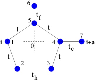
Figure 1: The pentagon unit cell. The numbers denote the n value, the in cell numbering of sites. The origin of the system of coordinates from where one analyses the cell is denoted by 0. The hopping matrix elements $t,t_{c},t_{h},t_{f}$are indicated on bonds, ${\bf i}$ denotes the lattice site to which the cell corresponds, and ${\bf a}$ is the lattice constant.

Concerning the technique used, it must be underlined Intr9 that contrary to the early stage of the method of the positive semidefinite operators where in the first step the ground state has been constructed, and the Hamiltonian adjusted to it (usually by extension terms in the Hamiltonian), the here used procedure starts from a given Hamiltonian, and deduce coherently the ground state corresponding to it without to know it a priory, and without to use extension terms. Concerning the pentagon chains, till now only nearest neighbor hoppings and the Hubbard interactions have been considered. The novelty in the present paper is that besides the Hamiltonian terms mentioned above, in deducing the exact ground states, we also consider SOI, nearest-neighbor Coulomb repulsion, and presence of external fields, from which the effect of the external magnetic field is considered both in its effect on the orbital motion of carriers (by Peierls phase factors), and its effect on the spin degrees of freedom (by the Zeeman term). In these conditions the paper focuses on the development of the technique such to construct a procedure which allows the treatment of the system in the presented circumstances. Hence one concentrates on the transformation of the Hamiltonian in positive semidefinite form, solution strategy of the matching equations, and construction process of the exact ground states, items, that for a coherent presentation need a given, and not negligible room. Hence, the presentation of the physical properties of the deduced ground states and phases is only sketched (I also note that this job needs extensive further supplementary study), the detailed presentation of the physical properties of the deduced exact ground states is left to a future publication. Nevertheless, the presented deduced physical properties underline a broad spectrum of interesting characteristics as e.g. emerging charge density wave phases, modification possibility of a static charge distribution by an external static magnetic field, switching possibilities between insulating and conducting phases by external magnetic fields, creation of effective flat bands provided not by the bare band structure, but by the two-particle local or non-local Coulomb interactions, peculiar ferromagnetic states, etc.

The remaining part of the paper is structured as follows: Section II presents the studied system, the transformation of the Hamiltonian in positive semidefinite form, and the solutions of the matching equations in the presence and absence of external fields. Section III presents the deduction procedure of the exact ground states, and the obtained ground states themselves. Section IV presents the summary and conclusions, while the attached six Appendices at the end of the paper contain the mathematical details.

II The system analyzed

II.1 The case of the zero external magnetic field

The Hamilton of the system is $\hat{H}=\hat{H}_{K}+\hat{H}_{U}+\hat{H}_{V}$, where one has

$$\hat{H}_{K} = \sum_{i}\sum_{\sigma,\sigma^{\prime}}[t^{\sigma,\sigma^{\prime}}(\hat{c}^{\dagger}_{i,1,\sigma}\hat{c}_{i,5,\sigma^{\prime}}+\hat{c}^{\dagger}_{i,2,\sigma}\hat{c}_{i,1,\sigma^{\prime}}+\hat{c}^{\dagger}_{i,4,\sigma}\hat{c}_{i,3,\sigma^{\prime}}+\hat{c}^{\dagger}_{i,5,\sigma}\hat{c}_{i,4,\sigma^{\prime}})+t_{h}^{\sigma,\sigma^{\prime}}\hat{c}^{\dagger}_{i,3,\sigma}\hat{c}_{i,2,\sigma^{\prime}}$$

$$+ t_{f}^{\sigma,\sigma^{\prime}}\hat{c}^{\dagger}_{i,6,\sigma}\hat{c}_{i,5,\sigma^{\prime}}+t_{c}^{\sigma,\sigma^{\prime}}\hat{c}^{\dagger}_{i+a,7,\sigma}\hat{c}_{i,4,\sigma^{\prime}}+h.c.]+\hat{H}_{\epsilon},\quad\hat{H}_{\epsilon}=\sum_{i,n}\epsilon^{\sigma,\sigma^{\prime}}\hat{c}^{\dagger}_{i,n,\sigma}\hat{c}_{i,n,\sigma^{\prime}},$$

$$\hat{H}_{U} = \sum_{i}\sum_{n=1,2,..6}U_{n}\hat{n}_{i,n}^{\uparrow}\hat{n}_{i,n}^{\downarrow},\quad\hat{H}_{V}=V\sum_{<i,j>}\sum_{<n,n^{\prime}>}\hat{n}_{i,n}\hat{n}_{j,n^{\prime}}$$ (1)

In Fig.1 one presents the unit cell of the system containing the in cell numbering of sites ($n$) in between 1 and 6. The hopping matrix elements, and the on-site one particle potentials have $(\sigma,\sigma^{\prime})$ spin projection indices in order to allow the presence of the many-body SOI. To match better the experimental situations, the antenna (describing the upper connected atoms), i.e. bond 5-6, the lower flank (bond 2-3), and the inter-cell connection (bond 4-7), are such taken to allow different hopping matrix elements, again for allowing comparison to different experimental realizations of the pentagon chain. The $\hat{H}_{\epsilon}$ term collects the on-site one particle potential terms. The $U_{n}>0$ coefficients are representing the on site Coulomb repulsions (Hubbard interaction), while $V\geq 0$ represents the nearest-neighbor Coulomb repulsion.

In order to transform in exact terms $\hat{H}$ in a positive semidefinite form, one introduces ten block operators $\hat{B}_{i,z,\sigma}$, $z=1,2,...5$ as follows:

$$\hat{B}_{i,1,\uparrow}=a_{1,1}\hat{c}_{i,1,\uparrow}+a_{1,2}\hat{c}_{i,2,\uparrow}+a_{1,5}\hat{c}_{i,5,\uparrow}+b_{1,1}\hat{c}_{i,1,\downarrow},$$

$$\hat{B}_{i,1,\downarrow}=a_{1,1}\hat{c}_{i,1,\downarrow}+a_{1,2}\hat{c}_{i,2,\downarrow}+a_{1,5}\hat{c}_{i,5,\downarrow}+b^{\prime}_{1,1}\hat{c}_{i,1,\uparrow},$$

$$\hat{B}_{i,2,\uparrow}=a_{2,2}\hat{c}_{i,2,\uparrow}+a_{2,3}\hat{c}_{i,3,\uparrow}+a_{2,5}\hat{c}_{i,5,\uparrow},$$

$$\hat{B}_{i,2,\downarrow}=a_{2,2}\hat{c}_{i,2,\downarrow}+a_{2,3}\hat{c}_{i,3,\downarrow}+a_{2,5}\hat{c}_{i,5,\downarrow},$$

$$\hat{B}_{i,3,\uparrow}=a_{3,3}\hat{c}_{i,3,\uparrow}+a_{3,4}\hat{c}_{i,4,\uparrow}+a_{3,5}\hat{c}_{i,5,\uparrow}+b_{3,4}\hat{c}_{i,4,\downarrow},$$

$$\hat{B}_{i,3,\downarrow}=a_{3,3}\hat{c}_{i,3,\downarrow}+a_{3,4}\hat{c}_{i,4,\downarrow}+a_{3,5}\hat{c}_{i,5,\downarrow}+b^{\prime}_{3,4}\hat{c}_{i,4,\uparrow},$$

$$\hat{B}_{i,4,\uparrow}=a_{4,5}\hat{c}_{i,5,\uparrow}+a_{4,6}\hat{c}_{i,6,\uparrow},$$

$$\hat{B}_{i,4,\downarrow}=a_{4,5}\hat{c}_{i,5,\downarrow}+a_{4,6}\hat{c}_{i,6,\downarrow},$$

$$\hat{B}_{i,5,\uparrow}=a_{5,4}\hat{c}_{i,4,\uparrow}+a_{5,7}\hat{c}_{i+a,7,\uparrow}+b_{5,4}\hat{c}_{i,4,\downarrow}+b_{5,7}\hat{c}_{i+a,7,\downarrow},$$

$$\hat{B}_{i,5,\downarrow}=a_{5,4}\hat{c}_{i,4,\downarrow}+a_{5,7}\hat{c}_{i+a,7,\downarrow}+b^{\prime}_{5,4}\hat{c}_{i,4,\uparrow}+b^{\prime}_{5,7}\hat{c}_{i+a,7,\uparrow}.$$ (2)

Here $i$ represents the lattice site, $z$ denotes the block operator index ($z=1,2,...5$), so $(z,\sigma)$ has 10 different values, while $\sigma$ represents the spin projection. The coefficients $a_{z,n}$ and $b_{z,n}$ called block operator parameters, are indexed by the block operator index $z$, and $n$, the on cell position on which the operator following the coefficient acts. The coefficients $a_{z,n}$ are present in terms whose spin projection is equal to the spin projection of the block operator, while the $b_{z,n}$ coefficients denote terms whose spin projection is opposite to the spin projection of the block operator. One has totally 21 block operator parameters ($a_{z,n}$ values: 13; and $b_{z,n}$ values: 8), which at the moment are unknown, but can be determined from the transformation of the starting Hamiltonian (1), to the positive semidefinite Hamiltonian

$$\hat{H}=\sum_{i,z,\sigma}\hat{B}^{\dagger}_{i,z,\sigma}\hat{B}_{i,z,\sigma}+\hat{H}_{U}+\hat{H}_{V}.$$ (3)

At this step I must note that the presented expression of the block operators in (2) has been optimized for the analyzed problem. This optimization has in fact two main aspects, namely: i) Because of the translational symmetry, the block operator parameters are the same in each unit cell, i.e. are $i$ independent. ii) The opposite spin components in the block operators are optimized in order to minimally describe the requirements raised by the presence of SOI which leads in fact to spin-flip hoppings. Given by this, we have much less $b_{z,n}$ coefficients in block operators than $a_{z,n}$ coefficients, which simplifies and helps the mathematical treatment.

If (3) is the same relation as (1), it must be a relationship in between the block operator parameters and the starting parameters of the Hamiltonian (1). These relations called the matching equations are presented in the following subsection.

II.2 Matching equations in zero external magnetic field.

The matching equations are obtained by effectuating the $\hat{B}^{\dagger}_{i,z,\sigma}\hat{B}_{i,z,\sigma}$ product together with the $\sum_{i,z,\sigma}$ sum operation in (3), and equating each obtained term to the corresponding term in (1). E.g. the coefficient of the operator $\hat{c}^{\dagger}_{i,1,\uparrow}\hat{c}_{i,5,\uparrow}$ in (3) is $a^{*}_{1,1}a_{1,5}$, while in (1) is $t_{1,5}^{\uparrow,\uparrow}$, the relation being spin projection independent, from where the third line of (4) follows, etc.

For the hoppings without spin-flip one obtains ten equations:

$$0=t^{\uparrow,\uparrow}_{2,5}=t^{\downarrow,\downarrow}_{2,5}=a^{*}_{1,2}a_{1,5}+a^{*}_{2,2}a_{2,5},$$

$$0=t^{\uparrow,\uparrow}_{3,5}=t^{\downarrow,\downarrow}_{3,5}=a^{*}_{3,3}a_{3,5}+a^{*}_{2,3}a_{2,5},$$

$$t=t^{\uparrow,\uparrow}_{1,5}=t^{\downarrow,\downarrow}_{1,5}=a^{*}_{1,1}a_{1,5},$$

$$t=t^{\uparrow,\uparrow}_{2,1}=t^{\downarrow,\downarrow}_{2,1}=a^{*}_{1,2}a_{1,1},$$

$$t=t^{\uparrow,\uparrow}_{4,3}=t^{\downarrow,\downarrow}_{4,3}=a^{*}_{3,4}a_{3,3},$$

$$t=t^{\uparrow,\uparrow}_{5,4}=t^{\downarrow,\downarrow}_{5,4}=a^{*}_{3,5}a_{3,4},$$

$$t_{h}=t^{\uparrow,\uparrow}_{3,2}=t^{\downarrow,\downarrow}_{3,2}=a^{*}_{2,3}a_{2,2},$$

$$t_{f}=t^{\uparrow,\uparrow}_{6,5}=t^{\downarrow,\downarrow}_{6,5}=a^{*}_{4,6}a_{4,5},$$

$$t_{c}=t^{\uparrow,\uparrow}_{c}=t^{\uparrow,\uparrow}_{7,4}=a^{*}_{5,7}a_{5,4}+{b^{\prime}}^{*}_{5,7}b^{\prime}_{5,4},$$

$$t_{c}=t^{\downarrow,\downarrow}_{c}=t^{\downarrow,\downarrow}_{7,4}=a^{*}_{5,7}a_{5,4}+b^{*}_{5,7}b_{5,4}.$$ (4)

The spin-flip hoppings provide also ten equations as follows

$$t^{\uparrow,\downarrow}_{1,5}={b^{\prime}}^{*}_{1,1}a_{1,5},$$

$$t^{\downarrow,\uparrow}_{1,5}=\frac{t^{\uparrow,\downarrow}_{1,5}}{\alpha}={b}^{*}_{1,1}a_{1,5},$$

$$t^{\uparrow,\downarrow}_{2,1}=a^{*}_{1,2}b_{1,1},$$

$$t^{\downarrow,\uparrow}_{2,1}=\frac{t^{\uparrow,\downarrow}_{2,1}}{\alpha}=a^{*}_{1,2}{b^{\prime}}_{1,1},$$

$$t^{\uparrow,\downarrow}_{5,4}=a^{*}_{3,5}b_{3,4},$$

$$t^{\downarrow,\uparrow}_{5,4}=\frac{t^{\uparrow,\downarrow}_{5,4}}{\alpha}=a^{*}_{3,5}{b^{\prime}}_{3,4},$$

$$t^{\uparrow,\downarrow}_{4,3}={b^{\prime}}^{*}_{3,4}a_{3,3},$$

$$t^{\downarrow,\uparrow}_{4,3}=\frac{t^{\uparrow,\downarrow}_{4,3}}{\alpha}=b^{*}_{3,4}{a}_{3,3},$$

$$t^{\uparrow,\downarrow}_{c}=t^{\uparrow,\downarrow}_{7,4}={b^{\prime}}^{*}_{5,7}a_{5,4}+a^{*}_{5,7}b_{5,4},$$

$$t^{\downarrow,\uparrow}_{c}=t^{\downarrow,\uparrow}_{7,4}=\frac{t^{\uparrow,\downarrow}_{7,4}}{\alpha_{c}}={b}^{*}_{5,7}a_{5,4}+a^{*}_{5,7}{b^{\prime}}_{5,4}.$$ (5)

In Eqs(5) the coefficients $\alpha,\alpha_{c}$ take into consideration the difference between the hoppings $t^{\uparrow,\downarrow}_{n,n^{\prime}}$ and $t^{\downarrow,\uparrow}_{n,n^{\prime}}$ given by the SOI. In the present case, taking into account only the Rashba term for conducting polymers Intr12 , one has $\alpha=\alpha_{c}=-1$.

The non spin-flip on-site one particle potentials provide eight matching equations which are as follows:

$$\epsilon_{4}=\epsilon^{\uparrow,\uparrow}_{6}=\epsilon^{\downarrow,\downarrow}_{6}=|a_{4,6}|^{2},$$

$$\epsilon_{3}=\epsilon^{\uparrow,\uparrow}_{5}=\epsilon^{\downarrow,\downarrow}_{5}=|a_{4,5}|^{2}+|a_{1,5}|^{2}+|a_{2,5}|^{2}+|a_{3,5}|^{2},$$

$$\epsilon_{2}=\epsilon^{\uparrow,\uparrow}_{2}=\epsilon^{\downarrow,\downarrow}_{2}=|a_{1,2}|^{2}+|a_{2,2}|^{2},$$

$$\epsilon_{2}=\epsilon^{\uparrow,\uparrow}_{3}=\epsilon^{\downarrow,\downarrow}_{3}=|a_{2,3}|^{2}+|a_{3,3}|^{2},$$

$$\epsilon_{1}=\epsilon^{\uparrow,\uparrow}_{1}=|a_{1,1}|^{2}+|a_{5,7}|^{2}+|b^{\prime}_{1,1}|^{2}+|b^{\prime}_{5,7}|^{2},$$

$$\epsilon_{1}=\epsilon^{\downarrow,\downarrow}_{1}=|a_{1,1}|^{2}+|a_{5,7}|^{2}+|b_{1,1}|^{2}+|b_{5,7}|^{2},$$

$$\epsilon_{1}=\epsilon^{\uparrow,\uparrow}_{4}=|a_{3,4}|^{2}+|a_{5,4}|^{2}+|b^{\prime}_{3,4}|^{2}+|b^{\prime}_{5,4}|^{2},$$

$$\epsilon_{1}=\epsilon^{\downarrow,\downarrow}_{4}=|a_{3,4}|^{2}+|a_{5,4}|^{2}+|b_{3,4}|^{2}+|b_{5,4}|^{2}.$$ (6)

For spin-flip on-site one particle potential one automatically has $\epsilon^{\uparrow,\downarrow}_{6}=\epsilon^{\downarrow,\uparrow}_{6}=0,\>$ $\epsilon^{\uparrow,\downarrow}_{5}=\epsilon^{\downarrow,\uparrow}_{5}=0,\>$ $\epsilon^{\uparrow,\downarrow}_{3}=\epsilon^{\downarrow,\uparrow}_{3}=0,\>$ $\epsilon^{\uparrow,\downarrow}_{2}=\epsilon^{\downarrow,\uparrow}_{2}=0,\>$ while $\epsilon^{\downarrow,\uparrow}_{1}=(\epsilon^{\uparrow,\downarrow}_{1})^{*},\>$ $\epsilon^{\downarrow,\uparrow}_{4}=(\epsilon^{\uparrow,\downarrow}_{4})^{*}$ is satisfied. The last two relations further provide two matching equations:

$$\epsilon^{\uparrow,\downarrow}_{1}=a^{*}_{1,1}b_{1,1}+a^{*}_{5,7}b_{5,7}+{b^{\prime}}^{*}_{1,1}a_{1,1}+{b^{\prime}}^{*}_{5,7}a_{5,7},$$

$$\epsilon^{\uparrow,\downarrow}_{4}=a^{*}_{3,4}b_{3,4}+a^{*}_{5,4}b_{5,4}+{b^{\prime}}^{*}_{3,4}a_{3,4}+{b^{\prime}}^{*}_{5,4}a_{5,4}.$$ (7)

The special treatment of $\epsilon^{\uparrow,\downarrow}_{1},\epsilon^{\uparrow,\downarrow}_{4}$ is motivated by the fact that the block operators connected to the bond $4-7$, or sites $1,4$ contain both spin projection components. But this is done only for the help of the mathematical treatment, and during the solving process of the matching equations, the left sides of Eqs.(7) will be considered zero.

Consequently, one has totally 30 matching equations. These are coupled, complex algebraic and non-linear equations, which must be solved for the block operator parameters in order to indeed transform in exact terms the Hamiltonian from Eq.(1), to the Hamiltonian from Eq.(3).

Having in mind the transformation to the Hamiltonian form from (3) one realizes, that based on the presented procedure another transformation of the Hamiltonian (1) in positive semidefinite form is possible (see Appendix A), namely

$$\hat{H}=\sum_{i,z,\sigma}\hat{B}_{i,z,\sigma}\hat{B}^{\dagger}_{i,z,\sigma}+\sum_{i}\sum_{n=1,2,..6}\hat{P}_{i,n}+\sum_{<l,k>}V\hat{R}_{<l,k>}+C,$$ (8)

where $C=q_{U}N-N_{c}\sum_{z,\sigma}y_{z,\sigma}-N_{c}\sum_{n=1,2,..6}U_{n}-28VN_{c}$, $N$ being the number of electrons, $N_{c}$ the number of lattice sites, $y_{z,\sigma}=\{\hat{B}_{i,z,\sigma},\hat{B}^{\dagger}_{i,z,\sigma}\}$ and $q_{U}$ being a constant which enters in the matching equations. In deducing $\hat{B}_{i,z,\sigma}$, the procedure described in this section must be applied, the results being identical, but the Hamiltonian parameters must be changed according to (54), namely $t^{\sigma,\sigma}_{i,j}\to-t^{\sigma,\sigma}_{i,j},\quad t^{\sigma,\sigma^{\prime}}_{i,j}\to-t^{\sigma,\sigma^{\prime}}_{i,j},\quad\epsilon^{\sigma,\sigma}_{i}\to q_{U}-(\epsilon^{\sigma,\sigma}_{i}+U_{i}+2Vr_{n}),\quad\epsilon^{\sigma,\sigma^{\prime}}\to-\epsilon^{\sigma,\sigma^{\prime}}$, where $\sigma\neq\sigma^{\prime}$ holds. Here, $\hat{P}_{i,n}=\hat{n}_{i,n}^{\uparrow}\hat{n}_{i,n}^{\downarrow}-(\hat{n}_{i,n}^{\uparrow}+\hat{n}_{i,n}^{\downarrow})+1$ represents a positive semidefinite operator which provides its minimum possible eigenvalue zero, when at least one electron is present at the site $(i,n)$ (i.e. lattice site i, and in-cell position n). Furthermore, $\hat{R}_{<l,k>}=\hat{n}_{l}\hat{n}_{k}-2(\hat{n}_{l}+\hat{n}_{k})+4$ is a positive semidefinite operator which provides its minimum possible eigenvalue zero, when the $l,k$ nearest neighbor sites are both at least once occupied, but such that at least one of them is doubly occupied.

At this step I must underline that a given starting Hamiltonian can be transformed in different positive semidefinite forms, each transformation placing the corresponding ground state in different regions of the parameter space Intr15 .

II.3 Solution of matching equations in zero external magnetic field.

The detailed solution of the matching equations is presented in Appendix B. The final result looks as follows:

$$a_{1,1}=\frac{|t|e^{i\theta_{1}}}{\sqrt{\epsilon_{2}-t_{h}}},\>a_{1,2}=a_{1,5}=sign(t)\sqrt{\epsilon_{2}-t_{h}}\>e^{i\theta_{1}},$$

$$a_{2,5}=-\frac{\epsilon_{2}-t_{h}}{\sqrt{t_{h}}}e^{i\theta_{2}},\>a_{2,2}=a_{2,3}=\sqrt{t_{h}}\>e^{i\theta_{2}},$$

$$a_{3,4}=\frac{|t|}{\sqrt{\epsilon_{2}-t_{h}}}e^{i\theta_{3}},\>a_{3,3}=a_{3,5}=sign(t)\sqrt{\epsilon_{2}-t_{h}}\>e^{i\theta_{3}},$$

$$a_{4,6}=\sqrt{\epsilon_{4}}\>e^{i\theta_{4}},\>a_{4,5}=\frac{t_{f}}{\sqrt{\epsilon_{4}}}\>e^{i\theta_{4}},$$

$$a_{5,4}=\frac{\sqrt{\gamma_{1}}}{\sqrt{1+\frac{(\sqrt{\gamma_{1}\gamma_{2}}-t_{c})^{2}}{{t^{\uparrow,\downarrow}_{c}}^{2}}}}e^{i\theta_{5}},\>a_{5,7}=\frac{\sqrt{\gamma_{2}}}{\sqrt{1+\frac{(\sqrt{\gamma_{1}\gamma_{2}}-t_{c})^{2}}{{t^{\uparrow,\downarrow}_{c}}^{2}}}}e^{i\theta_{5}},$$

$$b_{1,1}=sign(t)\frac{t_{2,1}^{\uparrow,\downarrow}}{\sqrt{\epsilon_{2}-t_{h}}}e^{i\theta_{1}},\>b^{\prime}_{1,1}=-sign(t)\frac{t_{2,1}^{\uparrow,\downarrow}}{\sqrt{\epsilon_{2}-t_{h}}}e^{i\theta_{1}},$$

$$b_{3,4}=sign(t)\frac{t_{5,4}^{\uparrow,\downarrow}}{\sqrt{\epsilon_{2}-t_{h}}}e^{i\theta_{3}},\>b^{\prime}_{3,4}=-sign(t)\frac{t_{5,4}^{\uparrow,\downarrow}}{\sqrt{\epsilon_{2}-t_{h}}}e^{i\theta_{3}},$$

$$b_{5,4}=\frac{\gamma_{1}\sqrt{\gamma_{2}}-t_{c}\sqrt{\gamma_{1}}}{t^{\uparrow,\downarrow}_{c}\sqrt{1+\frac{(\sqrt{\gamma_{1}\gamma_{2}}-t_{c})^{2}}{{t^{\uparrow,\downarrow}_{c}}^{2}}}}e^{i\theta_{5}},\>b^{\prime}_{5,4}=-\frac{\gamma_{1}\sqrt{\gamma_{2}}-t_{c}\sqrt{\gamma_{1}}}{t^{\uparrow,\downarrow}_{c}\sqrt{1+\frac{(\sqrt{\gamma_{1}\gamma_{2}}-t_{c})^{2}}{{t^{\uparrow,\downarrow}_{c}}^{2}}}}e^{i\theta_{5}},$$

$$b_{5,7}=\frac{t_{c}\sqrt{\gamma_{2}}-\gamma_{2}\sqrt{\gamma_{1}}}{t^{\uparrow,\downarrow}_{c}\sqrt{1+\frac{(\sqrt{\gamma_{1}\gamma_{2}}-t_{c})^{2}}{{t^{\uparrow,\downarrow}_{c}}^{2}}}}e^{i\theta_{5}},\>b^{\prime}_{5,7}=-\frac{t_{c}\sqrt{\gamma_{2}}-\gamma_{2}\sqrt{\gamma_{1}}}{t^{\uparrow,\downarrow}_{c}\sqrt{1+\frac{(\sqrt{\gamma_{1}\gamma_{2}}-t_{c})^{2}}{{t^{\uparrow,\downarrow}_{c}}^{2}}}}e^{i\theta_{5}},$$ (9)

where $\theta_{1},\theta_{2},...\theta_{5}$ are arbitrary phases. The deduced solution is placed in the following parameter space domain

$$\epsilon_{1}>0,\>\epsilon_{2}>0,\>\epsilon_{3}>0,\>\epsilon_{4}>0,\>t_{h}>0,\>\epsilon_{2}-t_{h}>0,$$

$$\gamma_{1}=\epsilon_{1}-\frac{t^{2}+{t^{\uparrow,\downarrow}_{2,1}}^{2}}{\epsilon_{2}-t_{h}}>0,\>\gamma_{2}=\epsilon_{1}-\frac{t^{2}+{t^{\uparrow,\downarrow}_{5,4}}^{2}}{\epsilon_{2}-t_{h}}>0,$$

$$\epsilon_{3}=\frac{t_{f}^{2}}{\epsilon_{4}}+\frac{\epsilon^{2}_{2}-t_{h}^{2}}{t_{h}},\>\gamma_{1}\gamma_{2}=t^{2}_{c}+{t^{\uparrow,\downarrow}_{c}}^{2}.$$ (10)

II.4 The case of the non-zero external magnetic field

We analyze also the case when an external magnetic field acts on the system perpendicular to the plane containing the polymer, i.e, perpendicular to the unit cell. The effect of the magnetic field is taken into account via i) the Peierls phase factors attached to the hopping matrix elements in describing the action on the orbital motion, and ii) the Zeeman term describing the effect on the spin degrees of freedom. In order to be explicitly clear, for $B\neq 0$ introducing the notation $\hat{H}_{1}=\hat{H}_{K}-\hat{H}_{\epsilon}$, one must transcribe carefully the $\hat{H}_{1}$ part of the one particle Hamiltonian as follows

$$\hat{H}_{1} = \sum_{i}\sum_{\sigma,\sigma^{\prime}}[t_{1,5}^{\sigma,\sigma^{\prime}}e^{i\phi_{1,5}}\hat{c}^{\dagger}_{i,1,\sigma}\hat{c}_{i,5,\sigma^{\prime}}+t_{2,1}^{\sigma,\sigma^{\prime}}e^{i\phi_{2,1}}\hat{c}^{\dagger}_{i,2,\sigma}\hat{c}_{i,1,\sigma^{\prime}}+t_{4,3}^{\sigma,\sigma^{\prime}}e^{i\phi_{4,3}}\hat{c}^{\dagger}_{i,4,\sigma}\hat{c}_{i,3,\sigma^{\prime}}+t_{5,4}^{\sigma,\sigma^{\prime}}e^{i\phi_{5,4}}\hat{c}^{\dagger}_{i,5,\sigma}\hat{c}_{i,4,\sigma^{\prime}}$$ (11)

$$+ t_{7,4}^{\sigma,\sigma^{\prime}}e^{i\phi_{7,4}}\hat{c}^{\dagger}_{i+a,7,\sigma}\hat{c}_{i,4,\sigma^{\prime}}+t_{3,2}^{\sigma,\sigma^{\prime}}e^{i\phi_{3,2}}\hat{c}^{\dagger}_{i,3,\sigma}\hat{c}_{i,2,\sigma^{\prime}}+t_{6,5}^{\sigma,\sigma^{\prime}}e^{i\phi_{6,5}}\hat{c}^{\dagger}_{i,6,\sigma}\hat{c}_{i,5,\sigma^{\prime}}+h.c.],$$

hence the total Hamiltonian becomes

$$\hat{H}=\hat{H}_{1}+\hat{H}_{\epsilon}+\hat{H}_{U}+\hat{H}_{V}+\hat{H}_{Z}.$$ (12)

For the Peierls phase factors one has $\phi_{3,2}=\phi_{1},\>\phi_{4,3}=\phi_{2,1}=\phi_{2},\>\phi_{5,4}=\phi_{1,5}=\phi_{3},\>\phi_{5,6}=\phi_{7,4}=0,$ and $\phi=\phi_{1}+2\phi_{2}+2\phi_{3}=2\pi\Phi/\Phi_{0}$, where $\Phi$ is the magnetic flux threading the unit cell, and $\Phi_{0}=hc/e$ is the flux quantum. Separately for each phase, one has $\phi_{\alpha}=2\pi BS_{\alpha}/\Phi_{0}$, where $\alpha=1,2,3$, furthermore $S_{1}=A(0,2,3),\>S_{2}=A(0,3,4),\>S_{3}=A(0,4,5)$, where $A(i,j,k)$ represents the area of the triangle defined by the points $(i,j,k)$ in Fig.1 presenting the unit cell. One trivially has $S=S_{1}+2S_{2}+2S_{3}$.

The Zeeman term in Eq.(12) has the standard form $\hat{H}_{Z}=-h\sum_{i,n}(\hat{n}_{i,n,\uparrow}-\hat{n}_{i,n,\downarrow})$. I note that $\hat{H}_{Z}$ maintains the structure of $\hat{H}$ since only it renormalizes the on-site one particle potentials in $\hat{H}_{\epsilon}$ by $\epsilon^{\sigma,\sigma}_{i}\to\epsilon^{\sigma,\sigma}_{i}+\mu h$, where $\mu=-1$ for $\sigma=\uparrow$ and $\mu=+1$ for $\sigma=\downarrow$.

II.5 Matching equations in non-zero external magnetic field.

In order to transform the Hamiltonian from (12) in positive semidefinite form one uses the same block operators as before, given in (2). The transformation in positive semidefinite form of the $\hat{H}$ can be given with the condition to consider in Eq.(2) different $a_{k,n}$ coefficients for $\hat{B}_{i,k,\uparrow}$ (these will be denoted by $a_{k,n,u}$) and $\hat{B}_{i,k,\downarrow}$ (these will be denoted by $a_{k,n,d}\neq a_{k,n,u}$), e.g.

$$\hat{B}_{i,1,\uparrow}=a_{1,1,u}\hat{c}_{i,1,\uparrow}+a_{1,2,u}\hat{c}_{i,2,\uparrow}+a_{1,5,u}\hat{c}_{i,5,\uparrow}+b_{1,1}\hat{c}_{i,1,\downarrow},$$

$$\hat{B}_{i,1,\downarrow}=a_{1,1,d}\hat{c}_{i,1,\downarrow}+a_{1,2,d}\hat{c}_{i,2,\downarrow}+a_{1,5,d}\hat{c}_{i,5,\downarrow}+b^{\prime}_{1,1}\hat{c}_{i,1,\uparrow},\>etc.$$ (13)

The transformation in the form positive semidefinite form given in (3), or (8) (with the conditions mentioned below (8)) requires the following matching equations:

The first ten matching equations from (4) for hoppings without spin-flip become now 18 equations (18, since also in Eq.(4) $t_{c}^{\uparrow,\uparrow}$ and $t_{c}^{\downarrow,\downarrow}$ had different equations) as follows

$$t^{\uparrow,\uparrow}_{1,5}e^{i\phi_{1,5}}=te^{i\phi_{3}}=a^{*}_{1,1,u}a_{1,5,u},$$

$$t^{\downarrow,\downarrow}_{1,5}e^{i\phi_{1,5}}=te^{i\phi_{3}}=a^{*}_{1,1,d}a_{1,5,d},$$

$$t^{\uparrow,\uparrow}_{2,1}e^{i\phi_{2,1}}=te^{i\phi_{2}}=a^{*}_{1,2,u}a_{1,1,u},$$

$$t^{\downarrow,\downarrow}_{2,1}e^{i\phi_{2,1}}=te^{i\phi_{2}}=a^{*}_{1,2,d}a_{1,1,d},$$

$$t^{\uparrow,\uparrow}_{4,3}e^{i\phi_{4,3}}=te^{i\phi_{2}}=a^{*}_{3,4,u}a_{3,3,u},$$

$$t^{\downarrow,\downarrow}_{4,3}e^{i\phi_{4,3}}=te^{i\phi_{2}}=a^{*}_{3,4,d}a_{3,3,d},$$

$$t^{\uparrow,\uparrow}_{5,4}e^{i\phi_{5,4}}=te^{i\phi_{3}}=a^{*}_{3,5,u}a_{3,4,u},$$

$$t^{\downarrow,\downarrow}_{5,4}e^{i\phi_{5,4}}=te^{i\phi_{3}}=a^{*}_{3,5,d}a_{3,4,d},$$

$$t^{\uparrow,\uparrow}_{3,2}e^{i\phi_{3,2}}=t_{h}e^{i\phi_{1}}=a^{*}_{2,3,u}a_{2,2,u},$$

$$t^{\downarrow,\downarrow}_{3,2}e^{i\phi_{3,2}}=t_{h}e^{i\phi_{1}}=a^{*}_{2,3,d}a_{2,2,d},$$

$$t^{\uparrow,\uparrow}_{6,5}e^{i\phi_{6,5}}=t_{f}=a^{*}_{4,6,u}a_{4,5,u},$$

$$t^{\downarrow,\downarrow}_{6,5}e^{i\phi_{6,5}}=t_{f}=a^{*}_{4,6,d}a_{4,5,d},$$

$$t^{\uparrow,\uparrow}_{7,4}e^{i\phi_{7,4}}=t_{c}=a^{*}_{5,7,u}a_{5,4,u}+{b^{\prime}}^{*}_{5,7}b^{\prime}_{5,4},$$

$$t^{\downarrow,\downarrow}_{7,4}e^{i\phi_{7,4}}=t_{c}=a^{*}_{5,7,d}a_{5,4,d}+b^{*}_{5,7}b_{5,4},$$

$$0=t^{\uparrow,\uparrow}_{2,5}=a^{*}_{1,2,u}a_{1,5,u}+a^{*}_{2,2,u}a_{2,5,u},$$

$$0=t^{\downarrow,\downarrow}_{2,5}=a^{*}_{1,2,d}a_{1,5,d}+a^{*}_{2,2,d}a_{2,5,d},$$

$$0=t^{\uparrow,\uparrow}_{3,5}=a^{*}_{3,3,u}a_{3,5,u}+a^{*}_{2,3,u}a_{2,5,u},$$

$$0=t^{\downarrow,\downarrow}_{3,5}=a^{*}_{3,3,d}a_{3,5,d}+a^{*}_{2,3,d}a_{2,5,d}.$$ (14)

The second group of ten matching equations relating the spin-flip contributions describing the SOI interaction, and substituting (5), become

$$t^{\uparrow,\downarrow}_{1,5}e^{i\phi_{1,5}}=-\lambda e^{i\phi_{3}}={b^{\prime}}^{*}_{1,1}a_{1,5,d},$$

$$t^{\downarrow,\uparrow}_{1,5}e^{i\phi_{1,5}}=\frac{t^{\uparrow,\downarrow}_{1,5}e^{i\phi_{1,5}}}{\alpha}=\lambda e^{i\phi_{3}}=={b}^{*}_{1,1}a_{1,5,u},$$

$$t^{\uparrow,\downarrow}_{2,1}e^{i\phi_{2,1}}=\lambda e^{i\phi_{2}}=a^{*}_{1,2,u}b_{1,1},$$

$$t^{\downarrow,\uparrow}_{2,1}e^{i\phi_{2,1}}=\frac{t^{\uparrow,\downarrow}_{2,1}e^{i\phi_{2,1}}}{\alpha}=-\lambda e^{i\phi_{2}}=a^{*}_{1,2,d}{b^{\prime}}_{1,1},$$

$$t^{\uparrow,\downarrow}_{5,4}e^{i\phi_{5,4}}=-\lambda e^{i\phi_{3}}=a^{*}_{3,5,u}b_{3,4},$$

$$t^{\downarrow,\uparrow}_{5,4}e^{i\phi_{5,4}}=\frac{t^{\uparrow,\downarrow}_{5,4}e^{i\phi_{5,4}}}{\alpha}=\lambda e^{i\phi_{3}}=a^{*}_{3,5,d}{b^{\prime}}_{3,4},$$

$$t^{\uparrow,\downarrow}_{4,3}e^{i\phi_{4,3}}=\lambda e^{i\phi_{2}}={b^{\prime}}^{*}_{3,4}a_{3,3,d},$$

$$t^{\downarrow,\uparrow}_{4,3}e^{i\phi_{4,3}}=\frac{t^{\uparrow,\downarrow}_{4,3}e^{i\phi_{4,3}}}{\alpha}=-\lambda e^{i\phi_{2}}=b^{*}_{3,4}{a}_{3,3,u},$$

$$t^{\uparrow,\downarrow}_{7,4}e^{i\phi_{4,7}}=\lambda_{c}={b^{\prime}}^{*}_{5,7}a_{5,4,d}+a^{*}_{5,7,u}b_{5,4},$$

$$t^{\downarrow,\uparrow}_{7,4}e^{i\phi_{7,4}}=\frac{t^{\uparrow,\downarrow}_{7,4}e^{i\phi_{7,4}}}{\alpha_{c}}=-\lambda_{c}={b}^{*}_{5,7}a_{5,4,u}+a^{*}_{5,7,d}{b^{\prime}}_{5,4}.$$ (15)

Here, taking into account symmetry considerations, we denoted the spin-flip hopping strengths by $\lambda$ and $\lambda_{c}$ according to the relations $t^{\uparrow,\downarrow}_{1,5}e^{i\phi_{1,5}}=-\lambda e^{i\phi_{3}},\>t^{\uparrow,\downarrow}_{5,4}e^{i\phi_{5,4}}=-\lambda e^{i\phi_{3}},\>t^{\uparrow,\downarrow}_{2,1}e^{i\phi_{2,1}}=\lambda e^{i\phi_{2}},\>t^{\uparrow,\downarrow}_{4,3}e^{i\phi_{4,3}}=\lambda e^{i\phi_{2}},\>t^{\uparrow,\downarrow}_{7,4}e^{i\phi_{7,4}}=\lambda_{c}e^{i\phi_{7,4}}=\lambda_{c}.$ Finally, the last ten matching equations provided by the on-site one-particle potentials are now 14 equations, as follows

$$\epsilon^{\uparrow,\uparrow}_{6}=\epsilon_{6}-h=|a_{4,6,u}|^{2},$$

$$\epsilon^{\downarrow,\downarrow}_{6}=\epsilon_{6}+h=|a_{4,6,d}|^{2},$$

$$\epsilon^{\uparrow,\uparrow}_{5}=\epsilon_{5}-h=|a_{4,5,u}|^{2}+|a_{1,5,u}|^{2}+|a_{2,5,u}|^{2}+|a_{3,5,u}|^{2},$$

$$\epsilon^{\downarrow,\downarrow}_{5}=\epsilon_{5}+h=|a_{4,5,d}|^{2}+|a_{1,5,d}|^{2}+|a_{2,5,d}|^{2}+|a_{3,5,d}|^{2},$$

$$\epsilon^{\uparrow,\uparrow}_{2}=\epsilon_{2}-h=|a_{1,2,u}|^{2}+|a_{2,2,u}|^{2},$$

$$\epsilon^{\downarrow,\downarrow}_{2}=\epsilon_{2}+h=|a_{1,2,d}|^{2}+|a_{2,2,d}|^{2},$$

$$\epsilon^{\uparrow,\uparrow}_{3}=\epsilon_{3}-h=|a_{2,3,u}|^{2}+|a_{3,3,u}|^{2},$$

$$\epsilon^{\downarrow,\downarrow}_{3}=\epsilon_{3}+h=|a_{2,3,d}|^{2}+|a_{3,3,d}|^{2},$$

$$\epsilon^{\uparrow,\uparrow}_{1}=\epsilon_{1}-h=|a_{1,1,u}|^{2}+|a_{5,7,u}|^{2}+|b^{\prime}_{1,1}|^{2}+|b^{\prime}_{5,7}|^{2},$$

$$\epsilon^{\downarrow,\downarrow}_{1}=\epsilon_{1}+h=|a_{1,1,d}|^{2}+|a_{5,7,d}|^{2}+|b_{1,1}|^{2}+|b_{5,7}|^{2},$$

$$\epsilon^{\uparrow,\uparrow}_{4}=\epsilon_{4}-h=|a_{3,4,u}|^{2}+|a_{5,4,u}|^{2}+|b^{\prime}_{3,4}|^{2}+|b^{\prime}_{5,4}|^{2},$$

$$\epsilon^{\downarrow,\downarrow}_{4}=\epsilon_{4}+h=|a_{3,4,d}|^{2}+|a_{5,4,d}|^{2}+|b_{3,4}|^{2}+|b_{5,4}|^{2},$$

$$\epsilon^{\uparrow,\downarrow}_{1}=0=a^{*}_{1,1,u}b_{1,1}+a^{*}_{5,7,u}b_{5,7}+{b^{\prime}}^{*}_{1,1}a_{1,1,d}+{b^{\prime}}^{*}_{5,7}a_{5,7,d},$$

$$\epsilon^{\uparrow,\downarrow}_{4}=0=a^{*}_{3,4,u}b_{3,4}+a^{*}_{5,4,u}b_{5,4}+{b^{\prime}}^{*}_{3,4}a_{3,4,d}+{b^{\prime}}^{*}_{5,4}a_{5,4,d},$$ (16)

where one has only 14 equations, since in Eqs.(6,7), the two equalities in (7) and the last four equalities from (6) (so totally six equalities) provide only six equations in (16), i.e. not multiplies.

Finally, one has in the ${\bf B}\neq 0$ case 42 coupled, non-linear complex algebraic matching equations. I only mention, that numerical software for solving such system of equations is not present today.

II.6 Solution of the matching equations in the presence of the external magnetic field

The matching equations at ${\bf B}\neq 0$ are solved in the Appendix C. The solution looks as follows:

In the case of the first eight block operators, the block operator parameters are given by the following relations: The coefficients of the $z=1$ block operators $\hat{B}_{i,z=1,\sigma}$ are given by

$$a_{1,1,u}=[\frac{t^{2}(T_{h}+\epsilon_{3}-h)}{(\epsilon_{2}-h)(\epsilon_{3}-h)-t_{h}^{2}}]^{1/2}e^{i\chi_{1,u}},\quad\quad a_{1,1,d}=[\frac{t^{2}(T_{h}+\epsilon_{3}+h)}{(\epsilon_{2}+h)(\epsilon_{3}+h)-t_{h}^{2}}]^{1/2}e^{i\chi_{1,d}},$$

$$a_{1,5,u}=te^{i\phi_{3}}[\frac{(\epsilon_{2}-h)(\epsilon_{3}-h)-t_{h}^{2}}{t^{2}(T_{h}+\epsilon_{3}-h)}]^{1/2}e^{i\chi_{1,u}},\quad a_{1,5,d}=te^{i\phi_{3}}[\frac{(\epsilon_{2}+h)(\epsilon_{3}+h)-t_{h}^{2}}{t^{2}(T_{h}+\epsilon_{3}+h)}]^{1/2}e^{i\chi_{1,d}},$$

$$a_{1,2,u}=te^{-i\phi_{2}}[\frac{(\epsilon_{2}-h)(\epsilon_{3}-h)-t_{h}^{2}}{t^{2}(T_{h}+\epsilon_{3}-h)}]^{1/2}e^{i\chi_{1,u}},\quad a_{1,2,d}=te^{-i\phi_{2}}[\frac{(\epsilon_{2}+h)(\epsilon_{3}+h)-t_{h}^{2}}{t^{2}(T_{h}+\epsilon_{3}+h)}]^{1/2}e^{i\chi_{1,d}},$$

$$b_{1,1}=\frac{\lambda}{t}\>[\frac{t^{2}(T_{h}+\epsilon_{3}-h)}{(\epsilon_{2}-h)(\epsilon_{3}-h)-t_{h}^{2}}]^{1/2}e^{i\chi_{1,u}},\quad b^{\prime}_{1,1}=-\frac{\lambda}{t}\>[\frac{t^{2}(T_{h}+\epsilon_{3}+h)}{(\epsilon_{2}+h)(\epsilon_{3}+h)-t_{h}^{2}}]^{1/2}e^{i\chi_{1,d}},$$ (17)

where $T_{h}=t_{h}e^{-i\phi}\geq 0$ must be satisfied. The coefficients of the $z=2$ block operators become

$$a_{2,2,u}=[\frac{(\epsilon_{3}-h)T_{h}+t_{h}^{2}}{T_{h}+\epsilon_{3}-h}]^{1/2}e^{i\chi_{2,u}},\quad\quad\quad a_{2,2,d}=[\frac{(\epsilon_{3}+h)T_{h}+t_{h}^{2}}{T_{h}+\epsilon_{3}+h}]^{1/2}e^{i\chi_{2,d}},$$

$$a_{2,3,u}=t_{h}e^{-i\phi_{1}}[\frac{T_{h}+\epsilon_{3}-h}{(\epsilon_{3}-h)T_{h}+t_{h}^{2}}]^{1/2}e^{i\chi_{2,u}},\quad a_{2,3,d}=t_{h}e^{-i\phi_{1}}[\frac{T_{h}+\epsilon_{3}+h}{(\epsilon_{3}+h)T_{h}+t_{h}^{2}}]^{1/2}e^{i\chi_{2,d}},$$

$$a_{2,5,u}=-e^{i(\phi_{2}+\phi_{3})}\frac{[(\epsilon_{2}-h)(\epsilon_{3}-h)-t_{h}^{2}]}{\sqrt{T_{h}(\epsilon_{2}-h)+t_{h}^{2}}\sqrt{\epsilon_{3}-h+T_{h}}}\>e^{i\chi_{2,u}},$$

$$a_{2,5,d}=-e^{i(\phi_{2}+\phi_{3})}\frac{[(\epsilon_{2}+h)(\epsilon_{3}+h)-t_{h}^{2}]}{\sqrt{T_{h}(\epsilon_{2}+h)+t_{h}^{2}}\sqrt{\epsilon_{3}+h+T_{h}}}\>e^{i\chi_{2,d}}.$$ (18)

The coefficients of the $z=3$ block operators become

$$a_{3,3,u}=te^{i\phi_{2}}\big{[}\frac{T_{h}[(\epsilon_{2}-h)(\epsilon_{3}-h)-t_{h}^{2}]}{t^{2}[T_{h}(\epsilon_{2}-h)+t_{h}^{2}]}\big{]}^{1/2}e^{i\chi_{3,u}},\quad a_{3,3,d}=te^{i\phi_{2}}\big{[}\frac{T_{h}[(\epsilon_{2}+h)(\epsilon_{3}+h)-t_{h}^{2}]}{t^{2}[T_{h}(\epsilon_{2}+h)+t_{h}^{2}]}\big{]}^{1/2}e^{i\chi_{3,d}},$$

$$a_{3,4,u}=\big{[}\frac{t^{2}[T_{h}(\epsilon_{2}-h)+t_{h}^{2}]}{T_{h}[(\epsilon_{2}-h)(\epsilon_{3}-h)-t_{h}^{2}]}\big{]}^{1/2}e^{i\chi_{3,u}},\quad a_{3,4,d}=\big{[}\frac{t^{2}[T_{h}(\epsilon_{2}+h)+t_{h}^{2}]}{T_{h}[(\epsilon_{2}+h)(\epsilon_{3}+h)-t_{h}^{2}]}\big{]}^{1/2}e^{i\chi_{3,d}},$$

$$a_{3,5,u}=te^{-i\phi_{3}}\big{[}\frac{T_{h}[(\epsilon_{2}-h)(\epsilon_{3}-h)-t_{h}^{2}]}{t^{2}[T_{h}(\epsilon_{2}-h)+t_{h}^{2}]}\big{]}^{1/2}e^{i\chi_{3,u}},\quad a_{3,5,d}=te^{-i\phi_{3}}\big{[}\frac{T_{h}[(\epsilon_{2}+h)(\epsilon_{3}+h)-t_{h}^{2}]}{t^{2}[T_{h}(\epsilon_{2}+h)+t_{h}^{2}]}\big{]}^{1/2}e^{i\chi_{3,d}},$$

$$b_{3,4}=-\frac{\lambda}{t}\big{[}\frac{t^{2}[T_{h}(\epsilon_{2}-h)+t_{h}^{2}]}{T_{h}[(\epsilon_{2}-h)(\epsilon_{3}-h)-t_{h}^{2}]}\big{]}^{1/2}e^{i\chi_{3,u}},\quad b^{\prime}_{3,4}=\frac{\lambda}{t}\big{[}\frac{t^{2}[T_{h}(\epsilon_{2}+h)+t_{h}^{2}]}{T_{h}[(\epsilon_{2}+h)(\epsilon_{3}+h)-t_{h}^{2}]}\big{]}^{1/2}e^{i\chi_{3,d}}.$$ (19)

The coefficients of the $z=4$ block operators are the following ones

$$a_{4,5,u}=\frac{t_{f}}{\sqrt{\epsilon_{6}-h}}e^{i\chi_{4,u}},\quad a_{4,5,d}=\frac{t_{f}}{\sqrt{\epsilon_{6}+h}}e^{i\chi_{4,d}},$$

$$a_{4,6,u}=\sqrt{\epsilon_{6}-h}e^{i\chi_{4,u}},\quad a_{4,6,d}=\sqrt{\epsilon_{6}+h}e^{i\chi_{4,d}}.$$ (20)

The calculation of the block operator coefficients connected to the block operators $\hat{B}_{i,5,\sigma}$, i.e. $z=5$ is much more tricky. First we should introduce the following notations

$$I_{1,u}=\epsilon_{1}-h-|a_{1,1,u}|^{2}-|b^{\prime}_{1,1}|^{2},\quad I_{1,d}=\epsilon_{1}+h-|a_{1,1,d}|^{2}-|b_{1,1}|^{2},$$

$$I_{2,u}=\epsilon_{4}-h-|a_{3,4,u}|^{2}-|b^{\prime}_{3,4}|^{2},\quad I_{2,d}=\epsilon_{4}+h-|a_{3,4,d}|^{2}-|b_{3,4}|^{2},$$

$$V_{1}=-a^{*}_{1,1,u}b_{1,1}-{b^{\prime}}^{*}_{1,1}a_{1,1,d},\quad V_{2}=-a^{*}_{3,4,u}b_{3,4}-{b^{\prime}}^{*}_{3,4}a_{3,4,d}.$$ (21)

Given by (17-20), all quantities from (21) have known and real values. Now, based on (21) one defines the expressions

$$W_{1}=\frac{t_{c}-zI_{1,u}}{V_{2}-z\lambda_{c}},\quad W_{2}=\frac{zt_{c}-I_{2,u}}{z\lambda_{c}-V_{2}},$$

$$W_{3}=\frac{t_{c}-yI_{1,d}}{V_{2}+y\lambda_{c}},\quad W_{4}=\frac{I_{2,d}-yt_{c}}{V_{2}+y\lambda_{c}},\quad y=\frac{z\lambda_{c}-V_{2}}{\lambda_{c}+zV_{1}}.$$ (22)

Based on (22) the following relations providing the requested remaining block operator parameters hold

$$b^{\prime}_{5,7}=W_{1}a_{5,4,d},\quad b^{\prime}_{5,4}=W_{2}a_{5,4,d},\quad b^{*}_{5,7}=W_{3}a^{*}_{5,4,u},\quad b^{*}_{5,4}=W_{4}a^{*}_{5,4,u},$$

$$a^{*}_{5,7,u}=\frac{a^{*}_{5,4,u}}{z},\quad a_{5,7,d}=\frac{a_{5,4,d}}{y}$$ (23)

The remaining two block operator parameters are given by

$$a_{5,4,u}=\big{[}\frac{V_{2}W_{1}-yV_{1}W_{2}}{W_{4}W_{1}-W_{3}W_{2}(y/z)}\big{]}^{1/2}e^{i\chi_{5,u}},\quad a_{5,4,d}=\big{[}\frac{V_{2}W_{3}-zV_{1}W_{4}}{W_{2}W_{3}-W_{1}W_{4}(z/y)}\big{]}^{1/2}e^{i\chi_{5,d}},$$ (24)

In the provided expressions Eqs.(17-24), the phases $\chi_{k,u},\chi_{k,d}$, $k=1,2,...5$ are arbitrary, and z is an arbitrary real parameter restricted by the conditions $|a_{5,4,u}|^{2},|a_{5,4,d}|^{2}>0$.

The parameter space region where the solution is valid is fixed by the relations $I_{\alpha,\nu}\geq 0$, where $\alpha=1,2$, $\nu=u,d$. These relations provide lower limits for the on-site one particle potentials $\epsilon_{1}$ and $\epsilon_{4}$. Furthermore on has $T_{h}\geq 0$, and two remaining matching equations from (16), namely $\epsilon_{5}+\mu(\nu)h=|a_{4,5,\nu}|^{2}+|a_{1,5,\nu}|^{2}+|a_{2,5,\nu}|^{2}+|a_{3,5,\nu}|^{2}$, where $\mu(u)=-1$ and $\mu(d)=+1$ which relates the $\epsilon_{5}$ value.

III Exact ground states

Once we solved the matching equations, the exact transformation of the Hamiltonian in positive semidefinite form has been performed. Now based on the positive semidefinite form of the Hamiltonian, one can deduce the exact ground states. This step will be done on two lines. First we deduce the exact ground state corresponding to the transformed Hamiltonian (3), and in the second step, the exact ground state corresponding to the transformed Hamiltonian from (8).

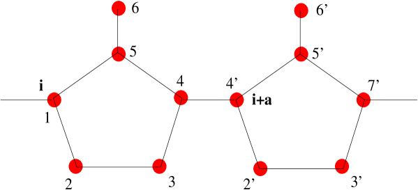
Figure 2: The $\hat{X}^{\dagger}_{i}$ operator connected to the lattice site ${\bf i}$. The red dotes denote the sites that are belong to $\hat{X}^{\dagger}_{i}$.

III.1 Ground states in the low density case

One concentrates now on the transformed Hamiltonian $\hat{H}$ from (3) used with periodic boundary conditions. The procedure is based on the deduction of a local operator $\hat{X}_{i}^{\dagger}$ that satisfy the property

$$\{\hat{B}_{j,z,\sigma},\hat{X}_{i}^{\dagger}\}=0$$ (25)

for all $j,i$ lattice sites, all $z=1,2,..5$, and all $\sigma$. The logic in this choice is that based on (25), one has for $|\Psi\rangle=\prod_{i}\hat{X}_{i}^{\dagger}|0\rangle$, where $|0\rangle$ is the vacuum state with no electrons present, the property

$$(\sum_{i,z,\sigma}\hat{B}^{\dagger}_{i,z,\sigma}\hat{B}_{i,z,\sigma})|\Psi\rangle=0$$ (26)

holds (since all $\hat{B}_{i,z,\sigma}$ can be interchanged with $\hat{X}_{i}^{\dagger}$). Consequently, introducing $|\Psi\rangle$ in the kernel of $\hat{H}_{U}$ (i.e. the Hilbert subspace provided by all $|\chi\rangle$ for which $\hat{H}_{U}|\chi\rangle=0$), and in the kernel of $\hat{H}_{V}$, one has the ground state.

In deducing $\hat{X}_{i}^{\dagger}$, one takes into consideration a most general domain defined on two unit cells, as presented in Fig.2. The operator is defined as

$$\hat{X}^{\dagger}_{i} = x^{*}_{1,\uparrow}\hat{c}^{\dagger}_{i,1,\uparrow}+x^{*}_{2,\uparrow}\hat{c}^{\dagger}_{i,2,\uparrow}+x^{*}_{3,\uparrow}\hat{c}^{\dagger}_{i,3,\uparrow}+x^{*}_{4,\uparrow}\hat{c}^{\dagger}_{i,4,\uparrow}+x^{*}_{5,\uparrow}\hat{c}^{\dagger}_{i,5,\uparrow}+x^{*}_{6,\uparrow}\hat{c}^{\dagger}_{6,1,\uparrow}+x^{*}_{4^{\prime},\uparrow}\hat{c}^{\dagger}_{i+1,1,\uparrow}$$ (27)

$$+ x^{*}_{2^{\prime},\uparrow}\hat{c}^{\dagger}_{i+1,2,\uparrow}+x^{*}_{3^{\prime},\uparrow}\hat{c}^{\dagger}_{i+1,3,\uparrow}+x^{*}_{5^{\prime},\uparrow}\hat{c}^{\dagger}_{i+1,5,\uparrow}+x^{*}_{6^{\prime},\uparrow}\hat{c}^{\dagger}_{i+1,6,\uparrow}+x^{*}_{7^{\prime},\uparrow}\hat{c}^{\dagger}_{i+1,4,\uparrow}+y^{*}_{1,\downarrow}\hat{c}^{\dagger}_{i,1,\downarrow}$$

$$+ y^{*}_{2,\downarrow}\hat{c}^{\dagger}_{i,2,\downarrow}+y^{*}_{3,\downarrow}\hat{c}^{\dagger}_{i,3,\downarrow}+y^{*}_{4,\downarrow}\hat{c}^{\dagger}_{i,4,\downarrow}+y^{*}_{5,\downarrow}\hat{c}^{\dagger}_{i,5,\downarrow}+y^{*}_{6,\downarrow}\hat{c}^{\dagger}_{i,6,\downarrow}+y^{*}_{4^{\prime},\downarrow}\hat{c}^{\dagger}_{i+1,1,\downarrow}+y^{*}_{2^{\prime},\downarrow}\hat{c}^{\dagger}_{i+1,2,\downarrow}$$

$$+ y^{*}_{3^{\prime},\downarrow}\hat{c}^{\dagger}_{i+1,3,\downarrow}+y^{*}_{5^{\prime},\downarrow}\hat{c}^{\dagger}_{i+1,5,\downarrow}+y^{*}_{6^{\prime},\downarrow}\hat{c}^{\dagger}_{i+1,6,\downarrow}+y^{*}_{7^{\prime},\downarrow}\hat{c}^{\dagger}_{i+1,4,\downarrow}.$$

Now the (25) anticommutators are presented, calculated in order with $\hat{B}_{i,1,\uparrow},\hat{B}_{i,1,\downarrow},\hat{B}_{i,2,\uparrow},\hat{B}_{i,2,\downarrow},...,\hat{B}_{i,5,\uparrow},\hat{B}_{i,5,\downarrow},\hat{B}_{i+1,1,\uparrow},\hat{B}_{i+1,1,\downarrow},\hat{B}_{i+1,2,\uparrow},\hat{B}_{i+1,2,\downarrow},...,\hat{B}_{i+1,5,\uparrow},\hat{B}_{i+1,5,\downarrow}$, $\hat{B}_{i-1,5,\uparrow},\hat{B}_{i-1,5,\downarrow}$, in total 22 equations

$$x^{*}_{2,\uparrow}a_{1,2,u}+x^{*}_{5,\uparrow}a_{1,5,u}+x^{*}_{1,\uparrow}a_{1,1,u}+y^{*}_{1,\downarrow}b_{1,1}=0,$$

$$y^{*}_{1,\downarrow}a_{1,1,d}+y^{*}_{5,\downarrow}a_{1,5,d}+y^{*}_{2,\downarrow}a_{1,2,d}+x^{*}_{1,\uparrow}b^{\prime}_{1,1}=0,$$

$$x^{*}_{2,\uparrow}a_{2,2,u}+x^{*}_{3,\uparrow}a_{2,3,u}+x^{*}_{5,\uparrow}a_{2,5,u}=0,$$

$$y^{*}_{3,\downarrow}a_{2,3,d}+y^{*}_{5,\downarrow}a_{2,5,d}+y^{*}_{2,\downarrow}a_{2,2,d}=0,$$

$$x^{*}_{3,\uparrow}a_{3,3,u}+x^{*}_{4,\uparrow}a_{3,4,u}+x^{*}_{5,\uparrow}a_{3,5,u}+y^{*}_{4,\downarrow}b_{3,4}=0,$$

$$y^{*}_{3,\downarrow}a_{3,3,d}+y^{*}_{4,\downarrow}a_{3,4,d}+y^{*}_{5,\downarrow}a_{3,5,d}+x^{*}_{4,\uparrow}b^{\prime}_{3,4}=0,$$

$$x^{*}_{5,\uparrow}a_{4,5,u}+x^{*}_{6,\uparrow}a_{4,6,u}=0,$$

$$y^{*}_{5,\downarrow}a_{4,5,d}+y^{*}_{6,\downarrow}a_{4,6,d}=0,$$

$$x^{*}_{4,\uparrow}a_{5,4,u}+x^{*}_{4^{\prime},\uparrow}a_{5,7,u}+y^{*}_{4,\downarrow}b_{5,4}+y^{*}_{4^{\prime},\downarrow}b_{5,7}=0,$$

$$x^{*}_{4,\uparrow}b^{\prime}_{5,4}+x^{*}_{4^{\prime},\uparrow}b^{\prime}_{5,7}+y^{*}_{4,\downarrow}a_{5,4,d}+y^{*}_{4^{\prime},\downarrow}a_{5,7,d}=0,$$

$$x^{*}_{4^{\prime},\uparrow}a_{1,1,u}+x^{*}_{2^{\prime},\uparrow}a_{1,2,u}+x^{*}_{5^{\prime},\uparrow}a_{1,5,u}+y^{*}_{4^{\prime},\downarrow}b_{1,1}=0,$$

$$x^{*}_{4^{\prime},\uparrow}b^{\prime}_{1,1}+y^{*}_{4^{\prime},\downarrow}a_{1,1,d}+y^{*}_{2^{\prime},\downarrow}a_{1,2,d}+y^{*}_{5^{\prime},\downarrow}a_{1,5,d}=0,$$

$$x^{*}_{2^{\prime},\uparrow}a_{2,2,u}+x^{*}_{3^{\prime},\uparrow}a_{2,3,u}+x^{*}_{5^{\prime},\uparrow}a_{2,5,u}=0,$$

$$y^{*}_{2^{\prime},\downarrow}a_{2,2,d}+y^{*}_{3^{\prime},\downarrow}a_{2,3,d}+y^{*}_{5^{\prime},\downarrow}a_{2,5,d}=0,$$

$$x^{*}_{3^{\prime},\uparrow}a_{3,3,u}+x^{*}_{5^{\prime},\uparrow}a_{3,5,u}+x^{*}_{7^{\prime},\uparrow}a_{3,4,u}+y^{*}_{7^{\prime},\downarrow}b_{3,4}=0,$$

$$y^{*}_{3^{\prime},\downarrow}a_{3,3,d}+y^{*}_{5^{\prime},\downarrow}a_{3,5,d}+x^{*}_{7^{\prime},\uparrow}b^{\prime}_{3,4}+y^{*}_{7^{\prime},\downarrow}a_{3,4,d}=0,$$

$$x^{*}_{5^{\prime},\uparrow}a_{4,5,u}+x^{*}_{6^{\prime},\uparrow}a_{4,6,u}=0,$$

$$y^{*}_{5^{\prime},\downarrow}a_{4,5,d}+y^{*}_{6^{\prime},\downarrow}a_{4,6,d}=0,$$

$$x^{*}_{7^{\prime},\uparrow}a_{5,4,u}+y^{*}_{7^{\prime},\downarrow}b_{5,4}=0,$$

$$x^{*}_{7^{\prime},\uparrow}b^{\prime}_{5,4}+y^{*}_{7^{\prime},\downarrow}a_{5,4,d}=0,$$

$$x^{*}_{1,\uparrow}a_{5,7,u}+y^{*}_{1,\downarrow}b_{5,7}=0,$$

$$x^{*}_{1,\uparrow}b^{\prime}_{5,7}+y^{*}_{1,\downarrow}a_{5,7,d}=0,$$ (28)

In the ${\bf B}=0$ case when $a_{i,j,u}=a_{i,j,d}=a_{i,j}$, $h=\phi=0$ holds, because of $b^{\prime}_{5,4}=-b_{5,4}$ and $b^{\prime}_{5,7}=-b_{5,7}$, (see (9)), the last four equations from (28) provide $x_{1,\uparrow}=y_{1,\downarrow}=x_{7^{\prime},\uparrow}=y_{7^{\prime},\downarrow}=0$, which is not satisfied automatically at ${\bf B}\neq 0$, i.e. $a_{i,j,u}\neq a_{i,j,d}$. That is why, (28) must be separately solved in the presence, and in the absence of the external magnetic field.

III.1.1 Solution for $\hat{X}^{\dagger}_{i}$ at $\hat{B}=0$

The solutions of (28) deduced in Appendix D, can be given as follows

$$x^{*}_{6,\uparrow}=\frac{t_{f}}{\epsilon_{4}}x^{*}_{2,\uparrow},\>x^{*}_{6^{\prime},\uparrow}=\frac{t_{f}}{\epsilon_{4}}x^{*}_{3^{\prime},\uparrow},\>x^{*}_{5,\uparrow}=-x^{*}_{2,\uparrow},\>x^{*}_{5^{\prime},\uparrow}=-x^{*}_{3^{\prime},\uparrow},\>x^{*}_{3,\uparrow}=\frac{-\epsilon_{2}}{t_{h}}x^{*}_{2,\uparrow},\>x^{*}_{1,\uparrow}=0,$$

$$x^{*}_{2^{\prime},\uparrow}=\frac{-\epsilon_{2}}{t_{h}}x^{*}_{3^{\prime},\uparrow},\>x^{*}_{4,\uparrow}=\frac{\epsilon_{2}^{2}-t^{2}_{h}}{t_{h}(t^{2}+\lambda^{2})}(tx^{*}_{2,\uparrow}-\lambda y^{*}_{2,\downarrow}),\>x^{*}_{4^{\prime},\uparrow}=\frac{\epsilon_{2}^{2}-t^{2}_{h}}{t_{h}(t^{2}+\lambda^{2})}(tx^{*}_{3^{\prime},\uparrow}-\lambda y^{*}_{3^{\prime},\downarrow}),$$

$$x^{*}_{7^{\prime},\uparrow}=0,\>y^{*}_{1,\downarrow}=0,\>y^{*}_{7^{\prime},\downarrow}=0,\>y^{*}_{6,\downarrow}=\frac{t_{f}}{\epsilon_{4}}y^{*}_{2,\downarrow},\>y^{*}_{6^{\prime},\downarrow}=\frac{t_{f}}{\epsilon_{4}}y^{*}_{3^{\prime},\downarrow},\>y^{*}_{5,\downarrow}=-y^{*}_{2,\downarrow},\>y^{*}_{5^{\prime},\downarrow}=-y^{*}_{3^{\prime},\downarrow},$$

$$y^{*}_{3,\downarrow}=-\frac{\epsilon_{2}}{t_{h}}y^{*}_{2,\downarrow},\>y^{*}_{2^{\prime},\downarrow}=-\frac{\epsilon_{2}}{t_{h}}y^{*}_{3^{\prime},\downarrow},\>y^{*}_{4,\downarrow}=\frac{\epsilon_{2}^{2}-t^{2}_{h}}{t_{h}(t^{2}+\lambda^{2})}(\lambda x^{*}_{2,\uparrow}+ty^{*}_{2,\downarrow}),$$

$$y^{*}_{4^{\prime},\downarrow}=\frac{\epsilon_{2}^{2}-t^{2}_{h}}{t_{h}(t^{2}+\lambda^{2})}(\lambda x^{*}_{3^{\prime},\uparrow}+ty^{*}_{3^{\prime},\downarrow}),$$ (29)

where the $t^{\uparrow,\downarrow}=\lambda$ notation has been introduced, where $\lambda$ represents the SOI coupling constant. From (29) is seen that all coefficients of $\hat{X}^{\dagger}_{i}$ have been expressed in function of $x^{*}_{2,\uparrow},x^{*}_{3^{\prime},\uparrow},y^{*}_{2,\downarrow},y^{*}_{3^{\prime},\downarrow}$. These can be deduced based on the following relations

$$x^{*}_{2,\uparrow}=\frac{-(\alpha\beta+\gamma\delta)x^{*}_{3^{\prime},\uparrow}+(\gamma\beta-\alpha\delta)y^{*}_{3^{\prime},\downarrow}}{\alpha^{2}+\gamma^{2}},\>y^{*}_{2,\downarrow}=\frac{-(\gamma\beta-\alpha\delta)x^{*}_{3^{\prime},\uparrow}-(\alpha\beta+\gamma\delta)y^{*}_{3^{\prime},\downarrow}}{\alpha^{2}+\gamma^{2}},$$ (30)

where $\alpha=ta_{5,4}+\lambda b_{5,4},\>\beta=ta_{5,7}+\lambda b_{5,7},\>\gamma=tb_{5,4}-\lambda a_{5,4},\>\delta=tb_{5,7}-\lambda a_{5,7}$, and $x^{*}_{3^{\prime},\uparrow}=p$, $y^{*}_{3^{\prime},\downarrow}=q$ are arbitrary parameters.

The physical meaning of these two free $p,q$ parameters can be given as follows: given two set values of these parameters: $p_{1},q_{1}$ and $p_{2},q_{2}$, one can construct two linearly independent $\hat{X}^{\dagger}_{i,1}$ and $\hat{X}^{\dagger}_{i,2}$ solutions, which provide two linearly independent Hilbert space vectors $|\Psi^{0}_{1}\rangle=\hat{X}^{\dagger}_{i,1}|0\rangle$, and $|\Psi^{0}_{2}\rangle=\hat{X}^{\dagger}_{i,2}|0\rangle$, where $|0\rangle$ is the vacuum state with no fermions present. These can be orthonormalized based on the Gram-Schmidt procedure

$$|\Psi_{1}\rangle=\frac{|\Psi^{0}_{1}\rangle}{\langle\Psi^{0}_{1}|\Psi^{0}_{1}\rangle},\quad|v\rangle=\langle\Psi^{0}_{2}|\Psi_{1}\rangle|\Psi_{1}\rangle,$$

$$|\Psi_{2}\rangle=\frac{|\Psi^{0}_{2}\rangle-|v\rangle}{(\langle\Psi^{0}_{2}|-\langle v|)(|\Psi^{0}_{2}\rangle-|v\rangle)},$$ (31)

obtaining $\langle\Psi_{1}|\Psi_{2}\rangle=0$ together with $\langle\Psi_{1}|\Psi_{1}\rangle=\langle\Psi_{2}|\Psi_{2}\rangle=1$. Please note that for this to be done, two free parameters are needed, since only one parameter, mathematically fixes the norm.

III.1.2 Solution for $\hat{X}^{\dagger}_{i}$ at $\hat{B}\neq 0$

The here presented solutions deduced in Appendix E occur at

$$a_{5,7,d}a_{5,7,u}\neq b_{5,7}b^{\prime}_{5,7},\quad a_{5,4,d}a_{5,4,u}\neq b_{5,4}b^{\prime}_{5,4},$$ (32)

where from the last four equations of (28) one has $x_{1,\uparrow}=x_{7^{\prime},\uparrow}=y_{1,\downarrow}=y_{7^{\prime},\uparrow}=0$. The deduced coefficients of the operator $\hat{X}^{\dagger}_{i}$ are as follows: The first 16 coefficients are given as

$$x^{*}_{6,\uparrow}=\frac{t_{f}}{\epsilon_{6}-h}e^{-i(\phi_{2}+\phi_{3})}x^{*}_{2,\uparrow},\>y^{*}_{6,\downarrow}=\frac{t_{f}}{\epsilon_{6}+h}e^{-i(\phi_{2}+\phi_{3})}y^{*}_{2,\downarrow},\>x^{*}_{6^{\prime},\uparrow}=\frac{t_{f}}{\epsilon_{6}-h}e^{i(\phi_{2}+\phi_{3})}x^{*}_{3^{\prime},\uparrow},$$

$$y^{*}_{6^{\prime},\downarrow}=\frac{t_{f}}{\epsilon_{6}+h}e^{i(\phi_{2}+\phi_{3})}y^{*}_{3^{\prime},\downarrow},\>x^{*}_{5,\uparrow}=-e^{-i(\phi_{2}+\phi_{3})}x^{*}_{2,\uparrow},\>y^{*}_{5,\downarrow}=-e^{-i(\phi_{2}+\phi_{3})}y^{*}_{2,\uparrow},\>x^{*}_{5^{\prime},\uparrow}=-e^{i(\phi_{2}+\phi_{3})}x^{*}_{3^{\prime},\uparrow},$$

$$y^{*}_{5^{\prime},\downarrow}=-e^{i(\phi_{2}+\phi_{3})}y^{*}_{3^{\prime},\downarrow},\>x^{*}_{3,\uparrow}=-e^{-i(2\phi_{2}+2\phi_{3})}\frac{\epsilon_{2}-h}{T_{h}}x^{*}_{2,\uparrow},\>y^{*}_{3,\downarrow}=-e^{-i(2\phi_{2}+2\phi_{3})}\frac{\epsilon_{2}+h}{T_{h}}y^{*}_{2,\downarrow},$$

$$x^{*}_{2^{\prime},\uparrow}=-e^{i(2\phi_{2}+2\phi_{3})}\frac{(\epsilon_{2}-h)(\epsilon_{3}-h)-t^{2}_{h}+T_{h}(T_{h}+\epsilon_{3}-h)}{T_{h}(\epsilon_{3}-h)+t^{2}_{h}}x^{*}_{3^{\prime},\uparrow},$$

$$y^{*}_{2^{\prime},\downarrow}=-e^{i(2\phi_{2}+2\phi_{3})}\frac{(\epsilon_{2}+h)(\epsilon_{3}+h)-t^{2}_{h}+T_{h}(T_{h}+\epsilon_{3}+h)}{T_{h}(\epsilon_{3}+h)+t^{2}_{h}}y^{*}_{3^{\prime},\downarrow},$$

$$y^{*}_{4,\downarrow}=ax^{*}_{2,\uparrow}+by^{*}_{2,\downarrow},\>x^{*}_{4,\uparrow}=cx^{*}_{2,\uparrow}+dy^{*}_{2,\downarrow},\>y^{*}_{4^{\prime},\downarrow}=a^{\prime}x^{*}_{3^{\prime},\uparrow}+b^{\prime}y^{*}_{3^{\prime},\downarrow},\>x^{*}_{4^{\prime},\uparrow}=c^{\prime}x^{*}_{3^{\prime},\uparrow}+d^{\prime}y^{*}_{3^{\prime},\downarrow},$$ (33)

where one has for the presented prefactors

$$a=-\lambda e^{-i(\phi_{2}+2\phi_{3})}J_{-},\>b=te^{-i(\phi_{2}+2\phi_{3})}J_{+},\>c=te^{-i(\phi_{2}+2\phi_{3})}J_{-},\>d=\lambda e^{-i(\phi_{2}+2\phi_{3})}J_{+},$$

$$a^{\prime}=\lambda e^{i(\phi_{2}+2\phi_{3})}J_{-},\>b^{\prime}=te^{i(\phi_{2}+2\phi_{3})}J_{+},\>c^{\prime}=te^{i(\phi_{2}+2\phi_{3})}J_{-},\>d^{\prime}=-\lambda e^{i(\phi_{2}+2\phi_{3})}J_{+},$$

$$J_{+}=\frac{(T_{h}+\epsilon_{2}+h)[(\epsilon_{2}+h)^{2}-t^{2}_{h}]}{(\lambda^{2}+t^{2})[T_{h}(\epsilon_{2}+h)+t^{2}_{h})]},\>J_{-}=\frac{(T_{h}+\epsilon_{2}-h)[(\epsilon_{2}-h)^{2}-t^{2}_{h}]}{(\lambda^{2}+t^{2})[T_{h}(\epsilon_{2}-h)+t^{2}_{h})]},$$ (34)

One notes that in (34) the $\epsilon_{2}=\epsilon_{3}$ equality has been used satisfying the symmetry properties of the system. All presented coefficients are expressed in function of the parameters $x^{*}_{2,\uparrow},x^{*}_{3^{\prime},\uparrow},y^{*}_{2,\downarrow},y^{*}_{3^{\prime},\downarrow}$. These are determined via

$$x^{*}_{2,\uparrow}=\frac{Y^{\prime}\beta^{\prime}-X^{\prime}\delta^{\prime}}{\gamma^{\prime}\beta^{\prime}-\alpha^{\prime}\delta^{\prime}},\>y^{*}_{2,\downarrow}=\frac{X^{\prime}\gamma^{\prime}-Y^{\prime}\alpha^{\prime}}{\gamma^{\prime}\beta^{\prime}-\alpha^{\prime}\delta^{\prime}},\>x^{*}_{3^{\prime},\uparrow}=p^{\prime},\>y^{*}_{3^{\prime},\downarrow}=q^{\prime},$$

$$\alpha^{\prime}=ca_{5,4,u}+ab_{5,4},\>\beta^{\prime}=da_{5,4,u}+bb_{5,4},\>\gamma^{\prime}=cb^{\prime}_{5,4}+aa_{5,4,d},\>\delta^{\prime}=db^{\prime}_{5,4}+ba_{5,4,d},$$

$$X^{\prime}=-p^{\prime}(a_{5,7,u}c^{\prime}+b_{5,7}a^{\prime})-q^{\prime}(a_{5,7,u}d^{\prime}+b_{5,7}b^{\prime}),$$

$$Y^{\prime}=-p^{\prime}(a_{5,7,d}a^{\prime}+b^{\prime}_{5,7}c^{\prime})-q^{\prime}(a_{5,7,d}b^{\prime}+b^{\prime}_{5,7}d^{\prime}),$$ (35)

where $p^{\prime},q^{\prime}$ are arbitrary parameters. I note that the denominator present on the first line of (35) is nonzero, since $\gamma^{\prime}\beta^{\prime}-\alpha^{\prime}\delta^{\prime}=e^{-2i(\phi_{2}+2\phi_{3})}J_{+}J_{-}(\lambda^{2}+t^{2})(b_{5,4}b^{\prime}_{5,4}-a_{5,4,d}a_{5,4,u})\neq 0$, see Eq.(32). Concerning $p^{\prime},q^{\prime}$ see the observation below (30) relating the $p,q$ parameters.

III.1.3 Other specific solutions for $\hat{X}^{\dagger}_{i}$

In the Appendix F we present two more specific solutions for $\hat{X}^{\dagger}_{i}$, one appearing i) in conditions when the requirement (32) is not satisfied, and ii) the domain on which $\hat{X}^{\dagger}_{i}$ is defined, differs from the domain presented in Fig.2. These solutions need supplementary interdependences in between the parameters of the Hamiltonian (e.g. (32) taken as equality). These new interdependences not diminish substantially the emergence possibilities of the phases described by the $\hat{X}^{\dagger}_{i}$ operators because e.g. the SOI coupling constants $\lambda,\lambda_{c}$ can be continuously tuned by external electric fields Intr3 .

III.1.4 The deduced exact ground states

Once the $\hat{X}^{\dagger}_{i}$ operators have been obtained, we deduce now the exact ground states for the Hamiltonian presented in (3).

For this reason let us consider the wave vector

$$|\Phi_{1}\rangle=\prod^{\prime}_{i}\hat{X}^{\dagger}_{i}|0\rangle=....\hat{X}^{\dagger}_{i}\hat{X}^{\dagger}_{i+2}\hat{X}^{\dagger}_{i+4}...|0\rangle$$ (36)

where $\prod^{\prime}_{i}$ represents a product on each second lattice site, and $\hat{X}^{\dagger}_{i}$ is taken from (29,30) deduced at ${\bf B}=0$. Note that $\hat{X}^{\dagger}_{i}$ places 1 electron on two nearest neighbor pentagons excepting their left and right end sites (sites 1 and 7’ in Fig.2). Inside the block covered by $\hat{X}^{\dagger}_{i}$ (sites 2,3,4,5,6,4’,2’,3’,5’,6’ in Fig.2), there are not present two electrons (i.e. double occupancy is not present), hence $\hat{H}_{U}|\Phi_{1}\rangle=0$ holds. Furthermore, inside this block there are not present two nearest neighboring sites occupied both at least once, so $\hat{H}_{V}|\Psi_{1}\rangle=0$ also holds. In between two nearest neighbor $\hat{X}^{\dagger}_{i}$ and $\hat{X}^{\dagger}_{i+2}$ operators two empty sites are present (the horizontal bonds starting to the right from the site 7’, and starting to the left from the site 1 in Fig.2), so on these sites $\hat{H}_{U}|\Phi_{1}\rangle=0$, and $\hat{H}_{V}|\Phi_{1}\rangle=0$ are also satisfied, consequently

$$(\hat{H}_{U}+\hat{H}_{V})|\Phi_{1}\rangle=0$$ (37)

is satisfied. But $\hat{X}^{\dagger}_{i}$ was deduced from the condition (26), so (37) type of relation is satisfied also for the first term of the Hamiltonian (3), as a consequence $\hat{H}|\Phi_{1}\rangle=0$ holds. But since $\hat{H}$ is build up only from positive semidefinite terms, zero is the smallest possible eigenvalue of $\hat{H}$. As a consequence $|\Phi_{1}\rangle=|\Phi_{g,1}\rangle$ is the ground state of $\hat{H}$ at a number of $N=N_{c}/2$ particles in the system. The system has totally $6N_{c}$ sites, so the maximum number of electrons in the system is $N_{max}=12N_{c}$, consequently $N_{c}/2$ carriers represent $N/N_{max}=1/24$ particle concentration (quarter filled lowest band). This concentration value is placed below system half filling ($6N_{c}$ electrons), that is why is called “ground state in the low density” case. Physically this state represents a charge density wave, since on all second horizontal bonds (e.g. bond 7’ to ${\bf i}+2{\bf a}$ in Fig.2) carriers are missing. This state is insulating. For the solution to occur, from the point of view of the two-particle interaction terms, $U_{n}>0$, $V>0$, but otherwise arbitrary are needed.

One more problem must be treated, namely the interplay between $|\Phi_{1}\rangle$ mentioned above, and $|\Psi_{\alpha}\rangle$, $\alpha=1,2$ presented in (31). For this to be understood, we must turn back to (9), which provide the solution of the matching equations used here, together with the conditions (10), these last providing the parameter space region where the solution is valid. Checking the conditions (10) for their meaning in the band structure [see Ref. Intr3 ], one sees, that it provides a lowest flat band, which is double degenerate. Consequently, in $|\Phi_{g,1}\rangle$ one can use at the sites i or $\hat{X}^{\dagger}_{i,1}$ or $\hat{X}^{\dagger}_{i,2}$, but not both, maintaining the quarter filling of the lowest band.

I must also underline that a ground state solution of the type (36) holds as well bellow $c_{0}=N/N_{max}=1/24$ system filling. In this case

$$|\Phi_{g,1}(c<c_{0})\rangle=\prod_{i\in D}\hat{X}^{\dagger}_{i}|0\rangle,$$ (38)

where $D$ is a lattice sites manifold containing $N<c_{0}N_{max}$ lattice sites $D={i_{1},i_{2},...i_{N}}$, where the sites contained in the $D$ domain must be at least at a distance $2{\bf a}$ from each other. In this case the charge density wave nature of the ground state is lost, and the ground state is built up from isolated clusters. The insulating nature of the system is maintained.

Now let us consider the ${\bf B}\neq 0$ case. In this situation one works with $\hat{X}^{\dagger}_{i}$ deduced in (33-35), and we consider here the $\hat{H}_{Z}=0$ case only, so only the effect of the external magnetic field on the orbital motion of electrons is considered described by the Peierls phase factors. In this case, at $c_{0}=1/24$ filling the ground state expression remains that given in (36), and at $c<c_{0}$ filling, that given in (38). But the situation is that the solution of the matching equations is satisfied only for fixed $\phi$ values (see Ref.Intr3 ). Hence when the magnetic field is switched on, the charge density wave phase disappears, and reappears at a fixed external magnetic field value. This is an interesting example which shows how a static magnetic fields can influence a static electric charge distribution. Furthermore, if (36) and (38) are not allowed solutions at $\phi\neq 0$, the lowest band will be dispersive, and the system becomes conducting. This provides a nice example demonstrating that a static magnetic field is able to turn an insulating phase to a conducting phase. The presented examples may have broad application possibilities in leading technologies.

When the conditions presented in the Appendix F.1 are satisfied, the expression of the ground state wave vectors from (36) and (38) remain valid at $V=0$ only, because in this case, along the horizontal bonds connecting the unit cells, two single occupied nearest neighbor sites can be present in the system. Because in this case also the sites 1 and 7’ in Fig.2 could be occupied, also the charge density wave nature of the ground state is lost.

When the conditions presented in the Appendix F.2 are present, the $\hat{X}^{\dagger}_{i}$ operator acts only on the four middle sites in each unit cell (2,3,5,6 in Fig.2). Now the (36), and (38) ground state expressions remain valid also at $V\neq 0$, and could contain even $N_{c}$ operators, so in this case the ground state can be written up to a carrier concentration $N/N_{max}=1/12$. One unit cell will be ferromagnetic, but the cells will be uncorrelated, so the ground state will be paramagnetic. A possible exception from this rule is provided by the situation when the lowest two bands touch each other: this situation will provide a ferromagnetic state based on a similar mechanism as described in Ref. Intr16 .

III.2 Ground states in the high density case.

The Hamiltonian one analyses now is presented in (8) used with periodic boundary conditions. The ground state construction now begins with

$$|\Phi^{\prime}_{1}\rangle=\prod^{N_{c}}_{i=1}\prod^{5}_{z=1}\prod_{\sigma=\uparrow,\downarrow}\hat{B}^{\dagger}_{i,z,\sigma}|0\rangle.$$ (39)

This strategy is based on the fact that $\hat{B}^{\dagger}_{i,z,\sigma}\hat{B}^{\dagger}_{i,z,\sigma}=0$, hence the first term from (8) satisfies

$$(\sum_{i,z,\sigma}\hat{B}_{i,z,\sigma}\hat{B}^{\dagger}_{i,z,\sigma})|\Phi^{\prime}_{1}\rangle=0.$$ (40)

The problem to be further solved now, is to introduce $|\Phi^{\prime}_{1}\rangle$ in the kernel of the remaining positive semidefinite operators from the Hamiltonian, i.e. $\sum_{i}\sum_{n=1,2,..6}U_{n}\hat{P}_{i,n}$ and $\sum_{<l,k>}V\hat{R}_{<l,k>}$. The first term from these two requires at least one electron on each site. The study of (39) shows that $|\Phi_{1}\rangle$ already introduces in the system $10N_{c}$ electrons, and with periodic boundary conditions this can leave one empty site per unit cell. So in order to do not have empty sites in the system, we must multiply the operators present in $|\Phi_{1}\rangle$ by a term

$$\hat{B}^{\dagger}=\prod_{i}c^{\dagger}_{i,n(i),\sigma(i)}(1-\hat{n}_{i,n(i),-\sigma(i)}),$$ (41)

which introduces in each unit cell one electron with an arbitrary spin $\sigma(i)$ on an arbitrary site $n(i)$, which is empty. The $\hat{B}^{\dagger}$ operator from (41) presents another novelty in comparison to its previous applications (see e.g. Ref. Intr8 ; Intr9 ; Intr10 ). Namely, together with the operators present in (39), preserves in the presented system only sites containing at least one electron, but supplementary such that two single occupied sites cannot be in nearest neighbor positions. Hence, the wave vector

$$|\Phi_{1}\rangle=(\prod^{N_{c}}_{i=1}\prod^{5}_{z=1}\prod_{\sigma=\uparrow,\downarrow}\hat{B}^{\dagger}_{i,z,\sigma})\hat{B}^{\dagger}|0\rangle,$$ (42)

has at least one electron on each site, consequently

$$(\sum_{i}\sum_{n=1,2,..6}U_{n}\hat{P}_{i,n})|\Phi_{1}\rangle=0,$$ (43)

holds. But besides this, one also has

$$(\sum_{<l,k>}V\hat{R}_{<l,k>})|\Phi_{1}\rangle=0,$$ (44)

because $|\Phi_{1}\rangle$ not only contains sites at least once occupied, but supplementary not contains single occupied states in nearest neighbor positions. Since $|\Phi_{1}\rangle$ also satisfies (40), so $(\hat{H}-C)|\Phi_{1}\rangle=0$, hence $|\Phi_{1}\rangle$ is the ground state of the system, i.e. $|\Phi_{g,1}\rangle=|\Phi_{1}\rangle$, and the ground state energy is $E_{g}=C$. Since now $N/N_{max}>5/6$ is above system half filling ($N/N_{max}=1/2$), the here presented ground state is called high density ground state.

The $\hat{B}_{i,z,\sigma}$ operators present in (42) are those defined in (2), the matching equations remain at ${\bf B}=0$ the relations (4-7) and at ${\bf B}\neq 0$ the equations (13-16), but with the substitutions presented in (54). Consequently, now the matching equations contain all coupling constants, including those present in SOI ($\lambda,\lambda_{c}$), in $\hat{H}_{U}$, and $\hat{H}_{V}$.

At ${\bf B}=0$ using for the block operator coefficients of $\hat{B}_{i,z,\sigma}$ deduced from (4-7), given by the conditions from (10), one finds again an effective flat band which is created not by the bare band structure, but by the $U,V$ interaction terms. The ground state $|\Phi_{g,1}\rangle$ presented in (42) is nonmagnetic, and corresponds to $c_{1}=N/N_{max}=11/12$ filling (upper band half filled). Turning on the external magnetic field, the mathematical expression of the deduced ground state remains the expression (42), but now the block operator parameters must be taken from the matching equations solution presented in (17- 24).

The ground state can be obtained also in the region $c_{1}<c\leq 1$. For this, in the case of the carrier concentration $c=(N_{1}+N^{\prime})/N_{max}$, where $N_{1}=c_{1}N_{max}$, and $1\leq N^{\prime}\leq N_{c})$, a supplementary operator $\hat{B}^{\dagger}_{c}=\prod_{j=1}^{N^{\prime}}\hat{c}^{\dagger}_{k_{j},\sigma_{j}}$ must be added to the operators present in (42), where $k_{j},\sigma_{j}$ are arbitrary momenta and spin projections. The ground state becomes in this case of the form

$$|\Phi_{g,1}(c>c_{1})\rangle=(\prod^{N_{c}}_{i=1}\prod^{5}_{z=1}\prod_{\sigma=\uparrow,\downarrow}\hat{B}^{\dagger}_{i,z,\sigma})\hat{B}^{\dagger}\hat{B}^{\dagger}_{c}|0\rangle,$$ (45)

which is a nonmagnetic and itinerant ground state.

IV Summary and conclusions

The paper analyses a pentagon chain type of conducting polymer in the presence of spin-orbit interactions SOI ($\lambda,\lambda_{c}$), on-site (U) and nearest neighbor (V) Coulomb repulsions, in the presence of external fields ${\bf E},{\bf B}$. Both fields are applied perpendicular to the plane containing the chain. ${\bf E}$ continuously tunes the SOI interaction strength, while the action of ${\bf B}$ is taken into account both at the level of the orbital motion of electrons (Peierls phase factors), and its action on the spin degrees of freedom (Zeeman term). Usually $\lambda<<U$ holds. Besides, if the SOI interaction strength is even small, it has essential effects on the physical properties of the system, since breaks the spin projection double degeneracy of each band. In these conditions, the perturbative description of the system in both small and high coupling constant limits is questionable, hence exact methods are used in the study. On the other side this job has its difficulties because the system is nonintegrable, so special technique must be applied in order to follow this route. On this line one uses the method based on positive semidefinite operator properties, which provides the first exact ground states for conducting polymers in the presence of SOI. Furthermore, for the first time this exact procedure is used in the case of conducting polymers in the presence of both U, and V Coulomb interactions. Besides, in this technique also for the first time the common action of ${\bf B}$ on spin and orbital degrees of freedom is considered. In these conditions the paper concentrates on the development of the technique used in the presented conditions: the transformation of the Hamiltonian in positive semidefinite form, the solution technique of the matching equations, the construction strategy of the exact ground states. The study of the physical properties of the deduced ground states is only sketched, since this job requires considerable future work, hence the detailed presentation of the physical properties of all deduced phases is left for a future publication. Even in these conditions, the presented physical properties show a broad spectrum of interesting physical characteristics as e.g. emerging charge density wave phases, modification possibility of a static charge distribution by an external static magnetic field, transition possibilities between insulating and conducting phases provided by external magnetic fields, emergence of effective flat bands provided by the two-particle local or non-local Coulomb interaction terms, peculiar ferromagnetic states, etc.

Appendix A Another transformation in positive semidefinite form

We wrote the system Hamiltonian from Eq.(1) in the form $\hat{H}=\hat{H}_{K}+\hat{H}_{U}+\hat{H}_{V}$. First we concentrate on the transformation of the $\hat{H}_{U}$ Hubbard term. It can be observed that

$$\hat{H}_{U} = \sum_{i}\sum_{n=1,2,..6}U_{n}\hat{n}_{i,n}^{\uparrow}\hat{n}_{i,n}^{\downarrow}=\sum_{i}\sum_{n=1,2,..6}U_{n}[\hat{n}_{i,n}^{\uparrow}\hat{n}_{i,n}^{\downarrow}-(\hat{n}_{i,n}^{\uparrow}+\hat{n}_{i,n}^{\downarrow})+1]$$ (46)

$$+ \sum_{i}\sum_{n=1,2,..6}U_{n}(\hat{n}_{i,n}^{\uparrow}+\hat{n}_{i,n}^{\uparrow})-\sum_{i}\sum_{n=1,2,..6}U_{n}=\sum_{i}\sum_{n=1,2,..6}U_{n}\hat{P}_{i,n}$$

$$+ \sum_{i}\sum_{n=1,2,..6}U_{n}(\hat{n}_{i,n}^{\uparrow}+\hat{n}_{i,n}^{\downarrow})-N_{c}\sum_{n=1,2,..6}U_{n},$$

where $N_{c}$ represents the number of lattice sites (cells), while $\hat{P}_{i,n}=[\hat{n}_{i,n}^{\uparrow}\hat{n}_{i,n}^{\downarrow}-(\hat{n}_{i,n}^{\uparrow}+\hat{n}_{i,n}^{\uparrow})+1]$ is a positive semidefinite operator which provides its minimum possible eigenvalue zero, when one has at least one electron on the $(i,n)$ site.

After this step one transforms the $\hat{H}_{V}$ term. For this, we introduce the site notation $(l,k)$ which cover all sites, not only the lattice sites. In these conditions, denoting the nearest neighbor $l,k$ sites (which are taken into consideration only once) by $<l,k>$, one has

$$\hat{H}_{V} = V\sum_{<k,l>}\hat{n}_{l}\hat{n}_{k}=V\sum_{<l,k>}[\hat{n}_{l}\hat{n}_{k}-2(\hat{n}_{l}+\hat{n}_{k})+4]+2V\sum_{<l,k>}(\hat{n}_{l}+\hat{n}_{k})$$ (47)

$$- 4\sum_{<l,k>}V=\sum_{<l,k>}V\hat{R}_{<l,k>}+\sum_{i}\sum_{n=1,2,..6}2Vr_{n}\hat{n}_{i,n}-28N_{c}V$$

where we have used the fact that 7 bonds are present in an unit cell, so $\sum_{<l,k>}=7\sum_{i}$ where i runs over the lattice sites, furthermore $\sum_{<l,k>}(\hat{n}_{l}+\hat{n}_{k})=\sum_{i}\sum_{n=1,2,..6}r_{n}\hat{n}_{i,n}$, where the coefficients $r_{1}=3,r_{2}=2,r_{3}=2,r_{4}=3,r_{5}=3,r_{6}=1$ show how many time a given site in an unit cell appears in the $\sum_{<l,k>}$ sum. Here the $\hat{R}_{<l,k>}=[\hat{n}_{l}\hat{n}_{k}-2(\hat{n}_{l}+\hat{n}_{k})+4]$ is a positive semidefinite operator which provides its minimum possible eigenvalue zero, when the $l,k$ nearest neighbor sites are at least once occupied, but such that at least one of them is doubly occupied.

Now we introduce in the Hamiltonian $\hat{H}$ from (1) the $\hat{H}_{U}$ term from (46) and the $\hat{H}_{V}$ term from (47) obtaining

$$\hat{H} = \hat{H}_{K}+(\sum_{i}\sum_{n=1,2,..6}U_{n}\hat{P}_{i,n}+\sum_{i}\sum_{n=1,2,..6}U_{n}(\hat{n}_{i,n}^{\uparrow}+\hat{n}_{i,n}^{\downarrow})-N_{c}\sum_{n=1,2,..6}U_{n})$$ (48)

$$+ (\sum_{<l,k>}V\hat{R}_{<l,k>}+\sum_{i}\sum_{n=1,2,..6}2Vr_{n}\hat{n}_{i,n}-28N_{c}V)$$

This Hamiltonian from Eq.(48) will be written in the positive semidefinite form

$$\hat{H}=\sum_{i,z,\sigma}\hat{B}^{\prime}_{i,z,\sigma}\hat{B}^{\prime\dagger}_{i,z,\sigma}+\sum_{i}\sum_{n=1,2,..6}U_{n}\hat{P}_{i,n}+\sum_{<l,k>}V\hat{R}_{<l,k>}+C$$ (49)

where $C$ is a constant, and $\hat{B}^{\prime}_{i,z,\sigma}$ has exactly the form presented in Eq.(2) with new coefficients. Denoting the anticommutators $\{\hat{B}^{\prime}_{i,z,\sigma},\hat{B}^{\prime\dagger}_{i,z,\sigma}\}=y_{z,\sigma}$ (note that $y_{z,\sigma}$ is the same in each cell placed at the lattice site i), Eq.(49) becomes of the form

$$\hat{H}=-\sum_{i,z,\sigma}\hat{B}^{\prime\dagger}_{i,z,\sigma}\hat{B}^{\prime}_{i,z,\sigma}+N_{c}\sum_{z,\sigma}y_{z,\sigma}+\sum_{i}\sum_{n=1,2,..6}U\hat{P}_{i,n}+\sum_{<l,k>}V\hat{R}_{<l,k>}+C$$ (50)

Now since the equations (48) and (50) contain the same Hamiltonian in the left side, equating the right sides on finds

$$\hat{H}_{K}+\sum_{i,\sigma}(U_{n}+2Vr_{n})\hat{n}_{i,n}^{\sigma}-q_{U}\sum_{i,\sigma}\hat{n}_{i,n}^{\sigma}+q_{U}N-N_{c}\sum_{n=1,2,..6}U_{n}-28N_{c}V=$$

$$-\sum_{i,z,\sigma}\hat{B}^{\prime\dagger}_{i,z,\sigma}\hat{B}^{\prime}_{i,z,\sigma}+N_{c}\sum_{z,\sigma}y_{z,\sigma}+C$$ (51)

where $N$ represents the number of electrons, and $q_{U}$ is a constant (note that we added to the left side $-q_{U}N+q_{U}N=0$). Now we deduce the block operators $\hat{B}^{\prime}_{i,z,\sigma}$ based on the transformation

$$\sum_{i,z,\sigma}\hat{B}^{\prime\dagger}_{i,z,\sigma}\hat{B}^{\prime}_{i,z,\sigma}=-[\hat{H}_{K}+\sum_{i,n,\sigma}(U_{n}+2Vr_{n})\hat{n}_{i,n}^{\sigma}-q_{U}\sum_{i,\sigma}\hat{n}_{i,n}^{\sigma}]$$ (52)

which taken into account in Eq.(51) provides for the constant $C$ the value

$$C=q_{U}N-N_{c}\sum_{z,\sigma}y_{z,\sigma}-N_{c}\sum_{n=1,2,..6}U_{n}-28VN_{c}$$ (53)

In conclusions, based on (49) the starting Hamiltonian from (1) can be transformed in the positive semidefinite form (49), where the constant $C$ is given in (53), and the block operator coefficient must be deduced based on (52).

But one realizes that the block operators $\hat{B}^{\prime}_{i,z,\sigma}$ are exactly the block operators $\hat{B}_{i,z,\sigma}$ from (2) whose matching equations are presented in Eqs.(4-7) with the condition that at the level of the Hamiltonian parameters the following changes are made

$$t^{\sigma,\sigma}_{i,j}\to-t^{\sigma,\sigma}_{i,j},\quad t^{\sigma,\sigma^{\prime}}_{i,j}\to-t^{\sigma,\sigma^{\prime}}_{i,j},\quad\epsilon^{\sigma,\sigma}_{i}\to q_{U}-(\epsilon^{\sigma,\sigma}_{i}+U_{i}+2Vr_{i}),\quad\epsilon^{\sigma,\sigma^{\prime}}\to-\epsilon^{\sigma,\sigma^{\prime}}$$ (54)

where $\sigma^{\prime}\neq\sigma$ holds. Hence with the changes from Eq.(54) the Hamiltonian from (1) becomes of the form

$$\hat{H}=\sum_{i,z,\sigma}\hat{B}_{i,z,\sigma}\hat{B}^{\dagger}_{i,z,\sigma}+\sum_{i}\sum_{n=1,2,..6}U_{n}\hat{P}_{i,n}+\sum_{<l,k>}V\hat{R}_{<l,k>}+C,$$ (55)

where the constant $C$ is given in (53), and the matching equations for the $\hat{B}_{i,z,\sigma}$ block operators defined in (2) remain does presented in Eqs.(4-7) at ${\bf B}=0$ and Eqs.(13- 16) at ${\bf B}\neq 0$ conditioned by the interchanges described in (54).

Appendix B Solution of the matching equations at $B=0$

B.0.1 The first ten equations.

One notes that during this solution one uses $t=t^{*}$, and concentrates on Eqs.(4). Since a solution of the matching equations is presented here for the first time in the paper, more details are mentioned during the presentation.

From the rows 3-8 of (4), six $a_{i,j}$ coefficients can be expressed in function of other $a_{i^{\prime},j^{\prime}}$ coefficients, reducing in this manner the number of unknown variables by six:

$$a_{1,5}=\frac{t}{a^{*}_{1,1}},\>a^{*}_{1,2}=\frac{t}{a_{1,1}},\>a_{3,3}=\frac{t}{a^{*}_{3,4}},\>a^{*}_{3,5}=\frac{t}{a_{3,4}},\>a^{*}_{2,3}=\frac{t_{h}}{a_{2,2}},\>a_{4,5}=\frac{t_{f}}{a^{*}_{4,6}},$$

$$a_{1,2}=a_{1,5},\quad a_{3,3}=a_{3,5}.$$ (56)

Using these relations, the remaining four equalities of (4) provide

$$t_{h}>0.$$ (57)

Indeed

$$a_{2,5}=-\frac{t^{2}}{a^{*}_{2,2}|a_{1,1}|^{2}},$$

$$t_{h}=\frac{|a_{2,2}|^{2}|a_{1,1}|^{2}}{|a_{3,4}|^{2}},\>=>\>|a_{3,4}|^{2}=\frac{|a_{2,2}|^{2}|a_{1,1}|^{2}}{t_{h}},$$

$$t_{c}=a^{*}_{5,7}a_{5,4}+b^{*}_{5,7}b_{5,4},$$

$$b^{*}_{5,7}b_{5,4}={b^{\prime}}^{*}_{5,7}b^{\prime}_{5,4},$$ (58)

The here obtained first two relations are such obtained, that one keeps the first equality of (4), and one divides the first two equalities of (4).

B.0.2 The second ten equations.

In what will follows on concentrates to Eqs.(5). The procedure used here is as follows: From consecutive two equations of (5) we form pairs. From the first component of the pair we express the $b$ coefficient. After this step by dividing the two components of the pair, one connects $b^{\prime}$ to $b$. In this manner, the following ten equations are obtained:

$${b^{\prime}}^{*}_{1,1}=\frac{t^{\uparrow,\downarrow}_{1,5}}{a_{1,5}},$$

$${b^{\prime}}^{*}_{1,1}=\alpha b^{*}_{1,1}$$

$$b_{1,1}=\frac{t^{\uparrow,\downarrow}_{2,1}}{a^{*}_{1,2}},$$

$$b_{1,1}=\alpha b^{\prime}_{1,1}$$

$$b_{3,4}=\frac{t^{\uparrow,\downarrow}_{5,4}}{a^{*}_{3,5}},$$

$$b_{3,4}=\alpha b^{\prime}_{3,4}$$

$${b^{\prime}}^{*}_{3,4}=\frac{t^{\uparrow,\downarrow}_{4,3}}{a_{3,3}},$$

$${b^{\prime}}^{*}_{3,4}=\alpha b^{*}_{3,4}$$

$$t^{\uparrow,\downarrow}_{c}={b^{\prime}}^{*}_{5,7}a_{5,4}+a^{*}_{5,7}b_{5,4},$$

$$\alpha_{c}=\frac{{b^{\prime}}^{*}_{5,7}a_{5,4}+a^{*}_{5,7}b_{5,4}}{{b}^{*}_{5,7}a_{5,4}+a^{*}_{5,7}{b^{\prime}}_{5,4}},$$ (59)

Now we divide the second and fourth line, and similarly the sixth and eight line respectively, obtaining

$$|b^{\prime}_{1,1}|^{2}=|b_{1,1}|^{2},\quad|b^{\prime}_{3,4}|^{2}=|b_{3,4}|^{2},\>=>\>|\alpha|^{2}=1$$ (60)

Introducing now the phase factors $\phi_{\alpha},\phi_{1},\phi_{2}$, based on (60), the following relations are obtained:

$$b^{\prime}_{1,1}=e^{i\phi_{1}}b_{1,1},\quad b^{\prime}_{3,4}=e^{i\phi_{2}}b_{3,4},\quad\alpha=e^{i\phi_{\alpha}},$$ (61)

But, from the fourth and sixth line of (59) one has $1=e^{i\phi_{\alpha}}e^{i\phi_{1}}$, and $1=e^{i\phi_{\alpha}}e^{i\phi_{2}}$ respectively, so

$$e^{i\phi_{1}}=e^{-i\phi_{\alpha}},\quad e^{i\phi_{2}}=e^{-i\phi_{\alpha}},$$ (62)

consequently, from (61) one obtains

$$b^{\prime}_{1,1}=e^{-i\phi_{\alpha}}b_{1,1},\quad b^{\prime}_{3,4}=e^{-i\phi_{\alpha}}b_{3,4}.$$ (63)

I further note that from (59), we further remain with the following relations

$$b_{1,1}=\frac{t^{\uparrow,\downarrow}_{2,1}}{a^{*}_{1,2}}=\frac{{t^{\uparrow,\downarrow}_{1,5}}^{*}}{a^{*}_{1,5}}e^{i\phi_{\alpha}},$$

$$b_{3,4}=\frac{t^{\uparrow,\downarrow}_{5,4}}{a^{*}_{3,5}}=\frac{{t^{\uparrow,\downarrow}_{4,3}}^{*}}{a^{*}_{3,3}}e^{i\phi_{\alpha}},$$

$$t^{\uparrow,\downarrow}_{c}={b^{\prime}}^{*}_{5,7}a_{5,4}+a^{*}_{5,7}b_{5,4},$$

$$\alpha_{c}=\frac{{b^{\prime}}^{*}_{5,7}a_{5,4}+a^{*}_{5,7}b_{5,4}}{{b}^{*}_{5,7}a_{5,4}+a^{*}_{5,7}{b^{\prime}}_{5,4}}.$$ (64)

Based on the second line of (8) we further have:

$$t^{\uparrow,\downarrow}_{2,1}={t^{\uparrow,\downarrow}_{1,5}}^{*}e^{i\phi_{\alpha}},\quad t^{\uparrow,\downarrow}_{5,4}={t^{\uparrow,\downarrow}_{4,3}}^{*}e^{i\phi_{\alpha}},$$ (65)

and what still remains to be analyzed from the second group of ten equations can be summarized as follows

$$b_{1,1}=\frac{t^{\uparrow,\downarrow}_{2,1}}{a^{*}_{1,2}},$$

$$b_{3,4}=\frac{t^{\uparrow,\downarrow}_{5,4}}{a^{*}_{3,5}},$$

$$t^{\uparrow,\downarrow}_{c}={b^{\prime}}^{*}_{5,7}a_{5,4}+a^{*}_{5,7}b_{5,4},$$

$$\alpha_{c}=\frac{{b^{\prime}}^{*}_{5,7}a_{5,4}+a^{*}_{5,7}b_{5,4}}{{b}^{*}_{5,7}a_{5,4}+a^{*}_{5,7}{b^{\prime}}_{5,4}},$$ (66)

B.0.3 The ten equations provided by the on-site one particle potentials.

3.a) The relations relating the b coefficients.

Taking into account that $\epsilon_{1}^{\uparrow,\uparrow}=\epsilon_{1}^{\downarrow,\downarrow}$, and $\epsilon_{4}^{\uparrow,\uparrow}=\epsilon_{4}^{\downarrow,\downarrow}$, based on the 5-6 and 7-8 equalities of (6), one finds

$$|b^{\prime}_{1,1}|^{2}+|b^{\prime}_{5,7}|^{2}=|b_{1,1}|^{2}+|b_{5,7}|^{2},$$

$$|b^{\prime}_{3,4}|^{2}+|b^{\prime}_{5,4}|^{2}=|b_{3,4}|^{2}+|b_{5,4}|^{2},$$ (67)

so taking into account (60), we find

$$|b^{\prime}_{5,7}|^{2}=|b_{5,7}|^{2},\quad|b^{\prime}_{5,4}|^{2}=|b_{5,4}|^{2}.$$ (68)

Now as in the case of (61), we introduce

$$b^{\prime}_{5,4}=e^{i\phi_{3}}b_{5,4},\quad b^{\prime}_{5,7}=e^{i\phi_{4}}b_{5,7}.$$ (69)

Introducing these results in the last equality of (58), one finds

$$b^{*}_{5,7}b_{5,4}=e^{-i\phi_{4}}b^{*}_{5,7}e^{i\phi_{3}}b_{5,4},\>=>\>e^{i\phi_{3}}=e^{i\phi_{4}}.$$ (70)

Introducing these results in the last equality of (66), one obtains

$$\alpha_{c}=\frac{e^{-i\phi_{3}}b^{*}_{5,7}a_{5,4}+a^{*}_{5,7}b_{5,4}}{b^{*}_{5,7}a_{5,4}+a^{*}_{5,7}b_{5,4}e^{i\phi_{3}}},\>=>\>\alpha_{c}=e^{-i\phi_{3}}\>=>\>\alpha_{c}=e^{i\phi_{\alpha_{c}}}=e^{-i\phi_{3}}.$$ (71)

After this step, using $\epsilon^{\sigma,-\sigma}_{i}=0,\>i=1,4$, the first two equalities of (7) provide information relating the $b_{5,4}$ and $b_{5,7}$ coefficients as follows

$$(a^{*}_{5,7}b_{5,7}+b^{*}_{5,7}a_{5,7}e^{i\phi_{\alpha_{c}}})=-(a^{*}_{1,1}b_{1,1}+b^{*}_{1,1}a_{1,1}e^{i\phi_{\alpha}}),$$

$$(a^{*}_{5,4}b_{5,4}+b^{*}_{5,4}a_{5,4}e^{i\phi_{\alpha_{c}}})=-(a^{*}_{3,4}b_{3,4}+b^{*}_{3,4}a_{3,4}e^{i\phi_{\alpha}}).$$ (72)

The obtained equalities (72) have an interesting structure, E.g. the first equality and its complex conjugate provide

$$(a^{*}_{5,7}b_{5,7}+b^{*}_{5,7}a_{5,7}e^{i\phi_{\alpha_{c}}})=-(a^{*}_{1,1}b_{1,1}+b^{*}_{1,1}a_{1,1}e^{i\phi_{\alpha}}),$$

$$(a_{5,7}b^{*}_{5,7}+b_{5,7}a^{*}_{5,7}e^{-i\phi_{\alpha_{c}}})=-(a_{1,1}b^{*}_{1,1}+b_{1,1}a^{*}_{1,1}e^{-i\phi_{\alpha}})\>=>$$

$$e^{-i\phi_{\alpha_{c}}}(a_{5,7}b^{*}_{5,7}e^{i\phi_{\alpha_{c}}}+b_{5,7}a^{*}_{5,7})=-e^{-i\phi_{\alpha}}(a_{1,1}b^{*}_{1,1}e^{i\phi_{\alpha}}+b_{1,1}a^{*}_{1,1}).$$ (73)

In this case based on the first row of (73), the third row will satisfy

$$e^{-i\phi_{\alpha_{c}}}=e^{-i\phi_{\alpha}},\>=>\>e^{i\phi_{\alpha_{c}}}=e^{i\phi_{\alpha}}.$$ (74)

Similar result is obtained from the second equality of (72), hence (72) can be written as

$$(a^{*}_{5,7}b_{5,7}+b^{*}_{5,7}a_{5,7}e^{i\phi_{\alpha}})=-(a^{*}_{1,1}b_{1,1}+b^{*}_{1,1}a_{1,1}e^{i\phi_{\alpha}}),$$

$$(a^{*}_{5,4}b_{5,4}+b^{*}_{5,4}a_{5,4}e^{i\phi_{\alpha}})=-(a^{*}_{3,4}b_{3,4}+b^{*}_{3,4}a_{3,4}e^{i\phi_{\alpha}}).$$ (75)

3.b) The relations relating the a coefficients

Now one analyses the equalities 3-4 of (6) in which we use as well (56) obtaining

$$\epsilon_{2}=\frac{t^{2}}{|a_{1,1}|^{2}}+|a_{2,2}|^{2},$$

$$\epsilon_{2}=\frac{t_{h}^{2}}{|a_{2,2}|^{2}}+\frac{t^{2}}{|a_{3,4}|^{2}},\>=>\>\epsilon_{2}=\frac{t_{h}^{2}}{|a_{2,2}|^{2}}+\frac{t^{2}t_{h}}{|a_{1,1}|^{2}|a_{2,2}|^{2}}$$ (76)

where in the last step one uses the second line of (58). From here, introducing the notations$X=\frac{t^{2}}{|a_{1,1}|^{2}}$, and $Y=|a_{2,2}|^{2}$ , the following system of linear equations is found

$$\epsilon_{2}=X+Y,$$

$$Y=\frac{t^{2}_{h}}{\epsilon_{2}}+\frac{t_{h}X}{\epsilon_{2}},$$ (77)

from where

$$X=\frac{t^{2}}{|a_{1,1}|^{2}}=\epsilon_{2}-t_{h},\>=>\>a_{1,1}=\frac{|t|e^{i\theta_{1}}}{\sqrt{\epsilon_{2}-t_{h}}},\>\epsilon_{2}>t_{h}>0,$$

$$Y=|a_{2,2}|^{2}=t_{h},\>=>\>a_{2,2}=\sqrt{t_{h}}e^{i\theta_{2}}.$$ (78)

Here, $\theta_{1},\theta_{2}$ are arbitrary phases. Now, from the first two equations of (58), one finds

$$a_{2,5}=-\frac{\epsilon_{2}-t_{h}}{\sqrt{t_{h}}}e^{i\theta_{2}},\quad a_{3,4}=\frac{|t|}{\sqrt{\epsilon_{2}-t_{h}}}e^{i\theta_{3}}$$ (79)

where again, $\theta_{3}$ is an arbitrary phase. One underlines, that after all these steps, from (57) only the third equation remains non-analyzed.

Now, using the first line of (6), from (56) one finds

$$a_{1,2}=a_{1,5}=sign(t)\sqrt{\epsilon_{2}-t_{h}}\>e^{i\theta_{1}},a_{3,3}=a_{3,5}=sign(t)\sqrt{\epsilon_{2}-t_{h}}\>e^{i\theta_{3}},$$

$$a_{2,2}=a_{2,3}=\sqrt{t_{h}}\>e^{i\theta_{2}},\>a_{4,6}=\sqrt{\epsilon_{4}}\>e^{i\theta_{4}},\>a_{4,5}=\frac{t_{f}}{\sqrt{\epsilon_{4}}}\>e^{i\theta_{4}},$$ (80)

where $\theta_{4}$ is an arbitrary phase.

3.c) The results relating the b coefficients

Using (63), the first two equalities of (66) provide

$$b_{1,1}=sign(t)\frac{t_{2,1}^{\uparrow,\downarrow}}{\sqrt{\epsilon_{2}-t_{h}}}e^{i\theta_{1}},\>b^{\prime}_{1,1}=e^{-i\phi_{\alpha}}b_{1,1},\>b_{3,4}=sign(t)\frac{t_{5,4}^{\uparrow,\downarrow}}{\sqrt{\epsilon_{2}-t_{h}}}e^{i\theta_{3}},\>b^{\prime}_{3,4}=e^{-i\phi_{\alpha}}b_{3,4},$$ (81)

One further notes, that from (66), only one equality remains to be analyzed, namely the third one.

3.d) The remaining equations

After these steps we underline, that till now only seven equations have not been used, namely, the following ones

$$t_{c}=a^{*}_{5,7}a_{5,4}+b^{*}_{5,7}b_{5,4},$$

$$t^{\uparrow,\downarrow}_{c}={b}^{*}_{5,7}a_{5,4}e^{i\phi_{\alpha}}+a^{*}_{5,7}b_{5,4},$$

$$(a^{*}_{5,7}b_{5,7}+b^{*}_{5,7}a_{5,7}e^{i\phi_{\alpha}})=-(a^{*}_{1,1}b_{1,1}+b^{*}_{1,1}a_{1,1}e^{i\phi_{\alpha}}),$$

$$(a^{*}_{5,4}b_{5,4}+b^{*}_{5,4}a_{5,4}e^{i\phi_{\alpha}})=-(a^{*}_{3,4}b_{3,4}+b^{*}_{3,4}a_{3,4}e^{i\phi_{\alpha}}),$$

$$\epsilon_{3}=\epsilon^{\uparrow,\uparrow}_{5}=\epsilon^{\downarrow,\downarrow}_{5}=|a_{4,5}|^{2}+|a_{1,5}|^{2}+|a_{2,5}|^{2}+|a_{3,5}|^{2},$$

$$\epsilon_{1}=\epsilon^{\downarrow,\downarrow}_{1}=|a_{1,1}|^{2}+|a_{5,7}|^{2}+|b_{1,1}|^{2}+|b_{5,7}|^{2},$$

$$\epsilon_{1}=\epsilon^{\downarrow,\downarrow}_{4}=|a_{3,4}|^{2}+|a_{5,4}|^{2}+|b_{3,4}|^{2}+|b_{5,4}|^{2}.$$ (82)

Introducing here the deduced results one finds the following system of equations

$$t_{c}=a^{*}_{5,7}a_{5,4}+b^{*}_{5,7}b_{5,4},$$

$$t^{\uparrow,\downarrow}_{c}={b}^{*}_{5,7}a_{5,4}e^{i\phi_{\alpha}}+a^{*}_{5,7}b_{5,4},$$

$$(a^{*}_{5,7}b_{5,7}+b^{*}_{5,7}a_{5,7}e^{i\phi_{\alpha}})=-\frac{t}{\epsilon_{2}-t_{h}}(t^{\uparrow,\downarrow}_{2,1}+{t^{\uparrow,\downarrow}_{2,1}}^{*}e^{i\phi_{\alpha}}),$$

$$(a^{*}_{5,4}b_{5,4}+b^{*}_{5,4}a_{5,4}e^{i\phi_{\alpha}})=-\frac{t}{\epsilon_{2}-t_{h}}(t^{\uparrow,\downarrow}_{5,4}+{t^{\uparrow,\downarrow}_{5,4}}^{*}e^{i\phi_{\alpha}}),$$

$$\epsilon_{3}=\frac{t_{f}^{2}}{\epsilon_{4}}+\frac{\epsilon^{2}_{2}-t_{h}^{2}}{t_{h}},$$

$$\epsilon_{1}-\frac{t^{2}+{t^{\uparrow,\downarrow}_{2,1}}^{2}}{\epsilon_{2}-t_{h}}=|a_{5,7}|^{2}+|b_{5,7}|^{2},$$

$$\epsilon_{1}-\frac{t^{2}+{t^{\uparrow,\downarrow}_{5,4}}^{2}}{\epsilon_{2}-t_{h}}=|a_{5,4}|^{2}+|b_{5,4}|^{2}.$$ (83)

In our case $t^{\uparrow,\downarrow}$ are real parameters, and $e^{i\phi_{\alpha}}=-1$ holds. Hence the third and fourth equations of (83) provide

$$a^{*}_{5,7}b_{5,7}=a_{5,7}b^{*}_{5,7},$$

$$a^{*}_{5,4}{b}_{5,4}=a_{5,4}b^{*}_{5,4}.$$ (84)

But this means that $a_{5,7},b_{5,7}$ have equal phases, and similarly, $a_{5,4},b_{5,4}$ have equal phases. I.e.

$$a_{5,7}=|a_{5,7}|e^{i\chi},\quad b_{5,7}=|b_{5,7}|e^{i\chi},$$

$$a_{5,4}=|a_{5,4}|e^{i\eta},\quad b_{5,4}=|b_{5,4}|e^{i\eta},$$ (85)

Introducing now (85) in the first equality of (83), one finds

$$t_{c}=|a_{5,7}|e^{-i\chi}|a_{5,4}|e^{i\eta}+|b_{5,7}|e^{-i\chi}|b_{5,4}|e^{i\eta},$$

$$\chi=\eta\pm 2n\pi,n\in N.$$ (86)

Now one introduces two notations, namely $\gamma_{1}$ and $\gamma_{2}$ defined as

$$\gamma_{1}=\epsilon_{1}-\frac{t^{2}+{t^{\uparrow,\downarrow}_{2,1}}^{2}}{\epsilon_{2}-t_{h}},$$

$$\gamma_{2}=\epsilon_{1}-\frac{t^{2}+{t^{\uparrow,\downarrow}_{5,4}}^{2}}{\epsilon_{2}-t_{h}}$$ (87)

In this manner, the first, and last two equations from (83) build up a closed system of equations

$$t_{c}=|a_{5,7}||a_{5,4}|+|b_{5,7}||b_{5,4}|,$$

$$t^{\uparrow,\downarrow}_{c}=|a_{5,7}||b_{5,4}|-|{b}_{5,7}||a_{5,4}|,$$

$$\gamma_{1}=|a_{5,7}|^{2}+|b_{5,7}|^{2},$$

$$\gamma_{2}=|a_{5,4}|^{2}+|b_{5,4}|^{2}.$$ (88)

In what will follows, we must solve the system of equations (88) In order to do this job, we must observe, that (88) not contains independent equations because it uses a relation in between the Hamiltonian parameters. Indeed, taking the square of the first two equations and adding them, one finds

$$|a_{5,7}|^{2}|a_{5,4}|^{2}+|b_{5,7}|^{2}|b_{5,4}|^{2}+|a_{5,7}|^{2}|b_{5,4}|^{2}+|b_{5,7}|^{2}|a_{5,4}|^{2}=t^{2}_{c}+{t^{\uparrow,\downarrow}_{c}}^{2},\>\to$$

$$|a_{5,7}|^{2}(|a_{5,4}|^{2}+|b_{5,4}|^{2})+|b_{5,7}|^{2}|(|a_{5,4}|^{2}+|b_{5,4}|^{2})=t^{2}_{c}+{t^{\uparrow,\downarrow}_{c}}^{2},\>\to$$

$$\gamma_{1}\gamma_{2}=t^{2}_{c}+{t^{\uparrow,\downarrow}_{c}}^{2}.$$ (89)

From the second equation of (88) $|b_{5,4}|=\frac{t_{c}^{\uparrow\downarrow}+|b_{5,7}||a_{5,4}|}{|a_{5,7}|}$, and this introduced in the first equality, allows to obtain the expression of $|b_{5,7}|$ in function of the $|a|$ coefficients. Using also the $\gamma_{2}$ expression, i.e. the fourth equation of (88), one obtains

$$|b_{5,7}|=\frac{t_{c}|a_{5,7}|-\gamma_{2}|a_{5,4}|}{t_{c}^{\uparrow\downarrow}}.$$ (90)

Similarly, from the second equation of (88) one has $|b_{5,7}|=\frac{-t_{c}^{\uparrow\downarrow}+|b_{5,4}||a_{5,7}|}{|a_{5,4}|}$. This introduced in the first equation one can express $|b_{5,7}|$ in function of $|a|$ parameters, and using the $\gamma_{1}$ expression from the third equation one finds

$$|b_{5,4}|=\frac{\gamma_{1}|a_{5,7}|-t_{c}|a_{5,4}|}{t_{c}^{\uparrow\downarrow}}.$$ (91)

In this moment the last two equations from (88) must be analyzed. Introducing here all previously deduced results, and introducing the notations $x=|a_{5,4}|$, $y=|a_{5,7}|$, the following system of equations are obtained

$$\gamma_{1}=x^{2}+\bigg{(}\frac{\gamma_{1}y-t_{c}x}{t_{c}^{\uparrow,\downarrow}}\bigg{)}^{2},$$

$$\gamma_{2}=y^{2}+\bigg{(}\frac{t_{c}y-\gamma_{2}x}{t_{c}^{\uparrow,\downarrow}}\bigg{)}^{2}.$$ (92)

Now it can be observed that the here obtained two equations, via $y\to\sqrt{\gamma_{2}/\gamma_{1}}\>x,\>x\to\sqrt{\gamma_{1}/\gamma_{2}}\>y$, transform in themselves, hence

$$|a_{5,7}|=y=\sqrt{\gamma_{2}/\gamma_{1}}\>x,\>x=|a_{5,4}|$$ (93)

Using (93)), the relation (91) can be written as

$$\gamma_{1}=x^{2}+\frac{x^{2}}{{t^{\uparrow,\downarrow}_{c}}^{2}}[\gamma_{1}\sqrt{\frac{\gamma_{2}}{\gamma_{1}}}-t_{c}]^{2}.$$ (94)

Based on (94) and using (89), one finds

$$|a_{5,4}|=x=\frac{\sqrt{\gamma_{1}}}{\sqrt{1+\frac{(\sqrt{\gamma_{1}\gamma_{2}}-t_{c})^{2}}{{t^{\uparrow,\downarrow}_{c}}^{2}}}},\quad|a_{5,7}|=y=\frac{\sqrt{\gamma_{2}}}{\sqrt{1+\frac{(\sqrt{\gamma_{1}\gamma_{2}}-t_{c})^{2}}{{t^{\uparrow,\downarrow}_{c}}^{2}}}},$$

$$\gamma_{1}\gamma_{2}=t^{2}_{c}+{t^{\uparrow,\downarrow}_{c}}^{2}.$$ (95)

B.1 Summary of the obtained results

B.1.1 The deduced block operator parameters.

The analyzed matching equations provided the following results:

$$a_{1,1}=\frac{|t|e^{i\theta_{1}}}{\sqrt{\epsilon_{2}-t_{h}}},\>a_{1,2}=a_{1,5}=sign(t)\sqrt{\epsilon_{2}-t_{h}}\>e^{i\theta_{1}},$$

$$a_{2,5}=-\frac{\epsilon_{2}-t_{h}}{\sqrt{t_{h}}}e^{i\theta_{2}},\>a_{2,2}=a_{2,3}=\sqrt{t_{h}}\>e^{i\theta_{2}},$$

$$a_{3,4}=\frac{|t|}{\sqrt{\epsilon_{2}-t_{h}}}e^{i\theta_{3}},\>a_{3,3}=a_{3,5}=sign(t)\sqrt{\epsilon_{2}-t_{h}}\>e^{i\theta_{3}},$$

$$a_{4,6}=\sqrt{\epsilon_{4}}\>e^{i\theta_{4}},\>a_{4,5}=\frac{t_{f}}{\sqrt{\epsilon_{4}}}\>e^{i\theta_{4}},$$

$$a_{5,4}=\frac{\sqrt{\gamma_{1}}}{\sqrt{1+\frac{(\sqrt{\gamma_{1}\gamma_{2}}-t_{c})^{2}}{{t^{\uparrow,\downarrow}_{c}}^{2}}}}e^{i\theta_{5}},\>a_{5,7}=\frac{\sqrt{\gamma_{2}}}{\sqrt{1+\frac{(\sqrt{\gamma_{1}\gamma_{2}}-t_{c})^{2}}{{t^{\uparrow,\downarrow}_{c}}^{2}}}}e^{i\theta_{5}},$$

$$b_{1,1}=sign(t)\frac{t_{2,1}^{\uparrow,\downarrow}}{\sqrt{\epsilon_{2}-t_{h}}}e^{i\theta_{1}},\>b^{\prime}_{1,1}=-sign(t)\frac{t_{2,1}^{\uparrow,\downarrow}}{\sqrt{\epsilon_{2}-t_{h}}}e^{i\theta_{1}},$$

$$b_{3,4}=sign(t)\frac{t_{5,4}^{\uparrow,\downarrow}}{\sqrt{\epsilon_{2}-t_{h}}}e^{i\theta_{3}},\>b^{\prime}_{3,4}=-sign(t)\frac{t_{5,4}^{\uparrow,\downarrow}}{\sqrt{\epsilon_{2}-t_{h}}}e^{i\theta_{3}},$$

$$b_{5,4}=\frac{\gamma_{1}\sqrt{\gamma_{2}}-t_{c}\sqrt{\gamma_{1}}}{t^{\uparrow,\downarrow}_{c}\sqrt{1+\frac{(\sqrt{\gamma_{1}\gamma_{2}}-t_{c})^{2}}{{t^{\uparrow,\downarrow}_{c}}^{2}}}}e^{i\theta_{5}},\>b^{\prime}_{5,4}=-\frac{\gamma_{1}\sqrt{\gamma_{2}}-t_{c}\sqrt{\gamma_{1}}}{t^{\uparrow,\downarrow}_{c}\sqrt{1+\frac{(\sqrt{\gamma_{1}\gamma_{2}}-t_{c})^{2}}{{t^{\uparrow,\downarrow}_{c}}^{2}}}}e^{i\theta_{5}},$$

$$b_{5,7}=\frac{t_{c}\sqrt{\gamma_{2}}-\gamma_{2}\sqrt{\gamma_{1}}}{t^{\uparrow,\downarrow}_{c}\sqrt{1+\frac{(\sqrt{\gamma_{1}\gamma_{2}}-t_{c})^{2}}{{t^{\uparrow,\downarrow}_{c}}^{2}}}}e^{i\theta_{5}},\>b^{\prime}_{5,7}=-\frac{t_{c}\sqrt{\gamma_{2}}-\gamma_{2}\sqrt{\gamma_{1}}}{t^{\uparrow,\downarrow}_{c}\sqrt{1+\frac{(\sqrt{\gamma_{1}\gamma_{2}}-t_{c})^{2}}{{t^{\uparrow,\downarrow}_{c}}^{2}}}}e^{i\theta_{5}}.$$ (96)

The deduced solution is placed in the following parameter domain

$$\epsilon_{1}>0,\>\epsilon_{2}>0,\>\epsilon_{3}>0,\>\epsilon_{4}>0,\>t_{h}>0,\>\epsilon_{2}-t_{h}>0,$$

$$\gamma_{1}=\epsilon_{1}-\frac{t^{2}+{t^{\uparrow,\downarrow}_{2,1}}^{2}}{\epsilon_{2}-t_{h}}>0,\>\gamma_{2}=\epsilon_{1}-\frac{t^{2}+{t^{\uparrow,\downarrow}_{5,4}}^{2}}{\epsilon_{2}-t_{h}}>0,$$

$$\epsilon_{3}=\frac{t_{f}^{2}}{\epsilon_{4}}+\frac{\epsilon^{2}_{2}-t_{h}^{2}}{t_{h}},\>\gamma_{1}\gamma_{2}=t^{2}_{c}+{t^{\uparrow,\downarrow}_{c}}^{2}.$$ (97)

I note that from symmetry considerations one has $t^{\uparrow,\downarrow}_{2,1}=t^{\uparrow,\downarrow}_{5,4}=t^{\uparrow,\downarrow}$, hence $\gamma_{1}=\gamma_{2}=\gamma$ holds

$$\gamma_{1}=\gamma_{2}=\gamma.$$ (98)

B.1.2 The check of the solutions of the matching equations

Using this matching equation solution, one exemplifies how the obtained results can be checked. First we check the obtained results for the $z=5$ block. One starts with the equation written for the $t_{c}$ hopping element.

$$t_{c}=a^{*}_{5,7}a_{5,4}+b^{*}_{5,7}b_{5,4}=\frac{\sqrt{\gamma_{1}\gamma_{2}}}{1+\frac{(\sqrt{\gamma_{1}\gamma_{2}}-t_{c})^{2}}{{t^{\uparrow,\downarrow}_{c}}^{2}}}+\frac{(\gamma_{1}\sqrt{\gamma_{2}}-t_{c}\sqrt{\gamma_{1}})(t_{c}\sqrt{\gamma_{2}}-\gamma_{2}\sqrt{\gamma_{1}})}{{t^{\uparrow,\downarrow}_{c}}^{2}(1+\frac{(\sqrt{\gamma_{1}\gamma_{2}}-t_{c})^{2}}{{t^{\uparrow,\downarrow}_{c}}^{2}})}=$$

$$\frac{{t^{\uparrow,\downarrow}_{c}}^{2}\sqrt{\gamma_{1}\gamma_{2}}+(2t_{c}\gamma_{1}\gamma_{2}-t^{2}_{c}\sqrt{\gamma_{1}\gamma_{2}}-\gamma_{1}\gamma_{2}\sqrt{\gamma_{1}\gamma_{2}})}{{t^{\uparrow,\downarrow}_{c}}^{2}+(\sqrt{\gamma_{1}\gamma_{2}}-t_{c})^{2}}=$$

$$\frac{(\gamma_{1}\gamma_{2}-t_{c}^{2})\sqrt{\gamma_{1}\gamma_{2}}+(2t_{c}\gamma_{1}\gamma_{2}-t^{2}_{c}\sqrt{\gamma_{1}\gamma_{2}}-\gamma_{1}\gamma_{2}\sqrt{\gamma_{1}\gamma_{2}})}{(\gamma_{1}\gamma_{2}-t^{2}_{c})+(\sqrt{\gamma_{1}\gamma_{2}}-t_{c})^{2}}=$$

$$\frac{t_{c}(2\gamma_{1}\gamma_{2}-2t_{c}\sqrt{\gamma_{1}\gamma_{2}})}{(2\gamma_{1}\gamma_{2}-2t_{c}\sqrt{\gamma_{1}\gamma_{2}})}=t_{c}$$ (99)

After this step the equation of $t^{\uparrow,\downarrow}_{c}$ follows:

$$t^{\uparrow,\downarrow}_{c}={b^{\prime}}^{*}_{5,7}a_{5,4}+a^{*}_{5,7}b_{5,4}=-\frac{(t_{c}\sqrt{\gamma_{2}}-\gamma_{2}\sqrt{\gamma_{1}})\sqrt{\gamma_{1}}}{t^{\uparrow,\downarrow}_{c}(1+\frac{(\sqrt{\gamma_{1}\gamma_{2}}-t_{c})^{2}}{{t^{\uparrow,\downarrow}_{c}}^{2}})}+\frac{(\gamma_{1}\sqrt{\gamma_{2}}-t_{c}\sqrt{\gamma_{1}})\sqrt{\gamma_{2}}}{t^{\uparrow,\downarrow}_{c}(1+\frac{(\sqrt{\gamma_{1}\gamma_{2}}-t_{c})^{2}}{{t^{\uparrow,\downarrow}_{c}}^{2}})}=$$

$$t^{\uparrow,\downarrow}_{c}\frac{(-t_{c}\sqrt{\gamma_{1}\gamma_{2}}+\gamma_{1}\gamma_{2})+(\gamma_{1}\gamma_{2}-t_{c}\sqrt{\gamma_{1}\gamma_{2}})}{{t^{\uparrow,\downarrow}_{c}}^{2}+(\sqrt{\gamma_{1}\gamma_{2}}-t_{c})^{2}}=t^{\uparrow,\downarrow}_{c}\frac{2\gamma_{1}\gamma_{2}-2t_{c}\sqrt{\gamma_{1}\gamma_{2}}}{(\gamma_{1}\gamma_{2}-t^{2}_{c})+(\sqrt{\gamma_{1}\gamma_{2}}-t_{c})^{2}}=$$

$$t^{\uparrow,\downarrow}_{c}\frac{2\gamma_{1}\gamma_{2}-2t_{c}\sqrt{\gamma_{1}\gamma_{2}}}{2\gamma_{1}\gamma_{2}-2t_{c}\sqrt{\gamma_{1}\gamma_{2}}}=t^{\uparrow,\downarrow}_{c}.$$ (100)

After this step one checks the two equations obtained for $\epsilon_{1}$, (see also (99))

$$\gamma=\gamma_{1}=|a_{5,7}|^{2}+|b_{5,7}|^{2}=\frac{\gamma_{2}}{1+\frac{(\sqrt{\gamma_{1}\gamma_{2}}-t_{c})^{2}}{{t^{\uparrow,\downarrow}_{c}}^{2}}}+\frac{(t_{c}\sqrt{\gamma_{2}}-\gamma_{2}\sqrt{\gamma_{1}})^{2}}{{t^{\uparrow,\downarrow}_{c}}^{2}(1+\frac{(\sqrt{\gamma_{1}\gamma_{2}}-t_{c})^{2}}{{t^{\uparrow,\downarrow}_{c}}^{2}})}=$$

$$\gamma_{2}\frac{{t^{\uparrow,\downarrow}_{c}}^{2}+(t^{2}_{c}+\gamma_{2}\gamma_{1}-2t_{c}\sqrt{\gamma_{2}\gamma_{1}})}{{t^{\uparrow,\downarrow}_{c}}^{2}+(\sqrt{\gamma_{2}\gamma_{1}}-t_{c})^{2}}=\gamma_{2}=\gamma.$$ (101)

Similar result is obtained from the second equality written for $\epsilon_{1}$ (see the last equality of (88))

And finally, the $\epsilon^{\uparrow,\downarrow}_{1}$ equation (see (7))

$$\epsilon^{\uparrow,\downarrow}_{1}=a^{*}_{1,1}b_{1,1}+a^{*}_{5,7}b_{5,7}+{b^{\prime}}^{*}_{1,1}a_{1,1}+{b^{\prime}}^{*}_{5,7}a_{5,7}=$$

$$|a_{1,1}||b_{1,1}|-|a_{1,1}||b_{1,1}|+|a_{5,7}||b_{5,7}|-|a_{5,7}||b_{5,7}|=0.$$ (102)

The other matching conditions are trivially satisfied.

B.1.3 Final results relating the block operator parameters

If one uses all the deduced results, including the symmetry considerations, the block operator parameters can be expressed in final form as follows:

$$a_{1,1}=\frac{|t|e^{i\theta_{1}}}{\sqrt{\epsilon_{2}-t_{h}}},\>a_{1,2}=a_{1,5}=sign(t)\sqrt{\epsilon_{2}-t_{h}}\>e^{i\theta_{1}},$$

$$a_{2,5}=-\frac{\epsilon_{2}-t_{h}}{\sqrt{t_{h}}}e^{i\theta_{2}},\>a_{2,2}=a_{2,3}=\sqrt{t_{h}}\>e^{i\theta_{2}},$$

$$a_{3,4}=\frac{|t|}{\sqrt{\epsilon_{2}-t_{h}}}e^{i\theta_{3}},\>a_{3,3}=a_{3,5}=sign(t)\sqrt{\epsilon_{2}-t_{h}}\>e^{i\theta_{3}},$$

$$a_{4,6}=\sqrt{\epsilon_{4}}\>e^{i\theta_{4}},\>a_{4,5}=\frac{t_{f}}{\sqrt{\epsilon_{4}}}\>e^{i\theta_{4}},$$

$$a_{5,4}=a_{5,7}=\sqrt{\frac{\gamma+t_{c}}{2}}e^{i\theta_{5}},$$

$$b_{1,1}=sign(t)\frac{t^{\uparrow,\downarrow}}{\sqrt{\epsilon_{2}-t_{h}}}e^{i\theta_{1}},\>b^{\prime}_{1,1}=-sign(t)\frac{t^{\uparrow,\downarrow}}{\sqrt{\epsilon_{2}-t_{h}}}e^{i\theta_{1}},$$

$$b_{3,4}=sign(t)\frac{t^{\uparrow,\downarrow}}{\sqrt{\epsilon_{2}-t_{h}}}e^{i\theta_{3}},\>b^{\prime}_{3,4}=-sign(t)\frac{t^{\uparrow,\downarrow}}{\sqrt{\epsilon_{2}-t_{h}}}e^{i\theta_{3}},$$

$$b_{5,4}=\frac{\gamma-t_{c}}{t^{\uparrow,\downarrow}_{c}}\sqrt{\frac{\gamma+t_{c}}{2}}e^{i\theta_{5}},\>b^{\prime}_{5,4}=-\frac{\gamma-t_{c}}{t^{\uparrow,\downarrow}_{c}}\sqrt{\frac{\gamma+t_{c}}{2}}e^{i\theta_{5}},$$

$$b_{5,7}=\frac{t_{c}-\gamma}{t^{\uparrow,\downarrow}_{c}}\sqrt{\frac{\gamma+t_{c}}{2}}e^{i\theta_{5}},\>b^{\prime}_{5,7}=-\frac{t_{c}-\gamma}{t^{\uparrow,\downarrow}_{c}}\sqrt{\frac{\gamma+t_{c}}{2}}e^{i\theta_{5}}.$$ (103)

The conditions under which the deduced solution hold (i.e. the parameter space domain where the solution is valid) can be given as follows

$$\epsilon_{1}>0,\>\epsilon_{4}>0,\>t_{h}>0,\>\epsilon_{2}-t_{h}>0,$$

$$\gamma=\epsilon_{1}-\frac{t^{2}+{t^{\uparrow,\downarrow}}^{2}}{\epsilon_{2}-t_{h}},\gamma+t_{c}>0,$$

$$\epsilon_{3}=\frac{t_{f}^{2}}{\epsilon_{4}}+\frac{\epsilon^{2}_{2}-t_{h}^{2}}{t_{h}},\>\gamma^{2}=t^{2}_{c}+{t^{\uparrow,\downarrow}_{c}}^{2}.$$ (104)

Appendix C Solution of the matching equations at $B\neq 0$

We start by (15) from where all b coefficients can be written in terms of the a coefficients

$${b^{\prime}}^{*}_{1,1}=-\frac{\lambda e^{i\phi_{3}}}{a_{1,5,d}},\>b^{*}_{1,1}=\frac{\lambda e^{i\phi_{3}}}{a_{1,5,u}},\>b^{*}_{1,1}=\frac{\lambda e^{i\phi_{2}}}{a^{*}_{1,2,u}},\>b^{\prime}_{1,1}=-\frac{\lambda e^{i\phi_{2}}}{a^{*}_{1,2,d}},\>b_{3,4}=-\frac{\lambda e^{i\phi_{3}}}{a^{*}_{3,5,u}},$$ (105)

$${b^{\prime}}_{3,4}=\frac{\lambda e^{i\phi_{3}}}{a^{*}_{3,5,d}},\>{b^{\prime}}^{*}_{3,4}=\frac{\lambda e^{i\phi_{2}}}{a_{3,3,d}},\>b^{*}_{3,4}=-\frac{\lambda e^{i\phi_{2}}}{a_{3,3,u}},\>{b^{\prime}}^{*}_{5,7}=\frac{\lambda_{c}-a^{*}_{5,7,u}b_{5,4}}{a_{5,4,d}},\>b^{\prime}_{5,4}=\frac{-\lambda_{c}-a_{5,4,u}b^{*}_{5,7}}{a^{*}_{5,7,d}},$$

so we can concentrate (at least up to the study of the last two bond operator parameters from (2)) to the $a_{i,j,\alpha}$ parameters.

Now, we write the first 12 equations from (61) in the following form

$$a_{1,5,u}=\frac{te^{i\phi_{3}}}{a^{*}_{1,1,u}},\>a^{*}_{1,2,u}=\frac{te^{i\phi_{2}}}{a_{1,1,u}},\>a_{1,5,d}=\frac{te^{i\phi_{3}}}{a^{*}_{1,1,d}},\>a^{*}_{1,2,d}=\frac{te^{i\phi_{2}}}{a^{*}_{1,1,d}},$$

$$a_{3,3,u}=\frac{te^{i\phi_{2}}}{a^{*}_{3,4,u}},\>a^{*}_{3,5,u}=\frac{te^{i\phi_{3}}}{a_{3,4,u}},\>a_{3,3,d}=\frac{te^{i\phi_{2}}}{a^{*}_{3,4,d}},\>a^{*}_{3,5,d}=\frac{te^{i\phi_{3}}}{a^{*}_{3,4,d}},$$

$$a^{*}_{2,3,u}=\frac{t_{h}e^{i\phi_{1}}}{a_{2,2,u}},\>a^{*}_{2,3,d}=\frac{t_{h}e^{i\phi_{1}}}{a_{2,2,d}},\>a_{4,5,u}=\frac{t_{f}}{a^{*}_{4,6,u}},\>a_{4,5,d}=\frac{t_{f}}{a^{*}_{4,6,d}}.$$ (106)

From the last two equations of (105) and the first two equations of (16) we automatically obtains

$$a_{4,5,u}=\frac{t_{f}e^{i\chi_{4,u}}}{\sqrt{\epsilon_{6}-h}},\>a_{4,5,d}=\frac{t_{f}e^{i\chi_{4,d}}}{\sqrt{\epsilon_{6}+h}},\>a_{4,6,u}=e^{i\chi_{4,u}}\sqrt{\epsilon_{6}-h},\>a_{4,6,d}=e^{i\chi_{4,d}}\sqrt{\epsilon_{6}+h},$$ (107)

where $\chi_{4,\nu}$, $\nu=u,d$ are arbitrary phases. So the $z=4$ block operator parameters have been deduced. One what will follows one concentrates on the $z=1,2,3$ block operators. We present in details the $\nu=u$ case, and underline that the deduction of the parameters in the $\nu=d$ case is done perfectly similarly.

One starts with the second and fourth equality from the bottom of (14) obtaining

$$a_{2,5,u}=-\frac{a^{*}_{1,2,u}a_{1,5,u}}{a^{*}_{2,2,u}}=-\frac{1}{a^{*}_{2,2,u}}\frac{t^{2}e^{i(\phi_{2}+\phi_{3})}}{|a_{1,1,u}|^{2}},$$

$$a^{*}_{2,5,u}=-\frac{a^{*}_{3,5,u}a_{3,3,u}}{a_{2,3,u}}=-\frac{1}{a_{2,3,u}}\frac{t^{2}e^{i(\phi_{2}+\phi_{3})}}{|a_{3,4,u}|^{2}}=-\frac{a^{*}_{2,2,u}}{t_{h}e^{-i\phi_{1}}}\frac{t^{2}e^{i(\phi_{2}+\phi_{3})}}{|a_{3,4,u}|^{2}},$$

$$|a_{2,5,u}|^{2}=\frac{t^{4}e^{i(\phi_{1}+2\phi_{2}+2\phi_{3})}}{t_{h}|a_{1,1,u}|^{2}|a_{3,4,u}|^{2}}=\frac{t^{4}}{T_{h}|a_{1,1,u}|^{2}|a_{3,4,u}|^{2}},\>T_{h}=\frac{|a_{2,2,u}|^{2}|a_{1,1,u}|^{2}}{|a_{3,4,u}|^{2}}.$$ (108)

where $T_{h}=t_{h}e^{-i\phi},\phi=\phi_{1}+2\phi_{2}+2\phi_{3}>0$ must hold. Here, in the first two rows we have used (107) as well, while in the last row, we multiplied the first two rows. I also mention, that from the second equality of the first row from (108) one has $|a_{2,5,u}|^{2}=t^{4}/(|a_{2,2,u}|^{2}|a_{1,1,u}|^{4})$, from where the last equality of (108) follows.

Now we use the 5th and 7th equation from (16), obtaining (in the last step, the last equality of (108) is used)

$$\epsilon_{2}-h=|a_{1,2,u}|^{2}+|a_{2,2,u}|^{2}=\frac{t^{2}}{|a_{1,1,u}|^{2}}+|a_{2,2,u}|^{2},$$

$$\epsilon_{3}-h=|a_{2,3,u}|^{2}+|a_{3,3,u}|^{2}=\frac{t_{h}^{2}}{|a_{2,2,u}|^{2}}+\frac{t^{2}}{|a_{3,4,u}|^{2}}=\frac{t_{h}^{2}}{|a_{2,2,u}|^{2}}+\frac{t^{2}T_{h}}{|a_{2,2,u}|^{2}|a_{1,1,u}|^{2}}.$$ (109)

From (109) now $a_{1,1,u},a_{2,2,u}$ can be expressed

$$a_{1,1,u}=\sqrt{\frac{t^{2}(\epsilon_{3}-h+T_{h})}{(\epsilon_{2}-h)(\epsilon_{3}-h)-t_{h}^{2})}}e^{i\chi_{1,u}},\quad a_{2,2,u}=\sqrt{\frac{T_{h}(\epsilon_{2}-h)+t_{h}^{2}}{\epsilon_{3}-h+T_{h}}}e^{i\chi_{2,u}}.$$ (110)

Based on the last two equations of (108) now $a_{3,4,u}$ (from the $T_{h}$ expression), then $a_{2,5,u}$ (from the first line of (108)) can be expressed

$$a_{3,4,u}=\sqrt{\frac{t^{2}[T_{h}(\epsilon_{2}-h)+t_{h}^{2}]}{T_{h}[(\epsilon_{2}-h)(\epsilon_{3}-h)-t_{h}^{2}]}}e^{i\chi_{3,u}},\>a_{2,5,u}=-e^{i(\phi_{2}+\phi_{3})}\frac{e^{i\chi_{2,u}}[(\epsilon_{2}-h)(\epsilon_{3}-h)-t_{h}^{2}]}{\sqrt{T_{h}(\epsilon_{2}-h)+t_{h}^{2}}\sqrt{\epsilon_{3}-h+T_{h}}}.$$ (111)

At this moment $a_{1,2,u},a_{1,5,u},a_{2,3,u},a_{3,4,u},a_{3,5,u}$ can be deduced from (106), while $b_{1,1},b_{3,4}$ are directly obtained from (105).

Starting from the 6th and 8th equalities of (16),and the first and third equality from the bottom of (14) a similar deduction provides the coefficients with index d, for z=1,2,3.

In the case of the block eoperator coefficients connected to the bond 4-7, namely the z=5 block operators, the procedure is more complicated, and different. The used equations in this case are the last six equalities from (16), the last two equalities of (15) and the two equations containing $t_{c}$ from (14). These equations can be written as

$$I_{1,u}=|a_{5,7,u}|^{2}+|b^{\prime}_{5,7}|^{2},\quad I_{1,d}=|a_{5,7,d}|^{2}+|b_{5,7}|^{2},$$

$$I_{2,u}=|a_{5,4,u}|^{2}+|b^{\prime}_{5,4}|^{2},\quad I_{2,d}=|a_{5,4,d}|^{2}+|b_{5,4}|^{2},$$

$$V_{1}=a^{*}_{5,7,u}b_{5,7}+{b^{\prime}}^{*}_{5,7}a_{5,7,d},\quad V_{2}=a^{*}_{5,4,u}b_{5,4}+{b^{\prime}}^{*}_{5,4}a_{5,4,d},$$

$$\lambda_{c}={b^{\prime}}^{*}_{5,7}a_{5,4,d}+a^{*}_{5,7,u}b_{5,4},\quad-\lambda_{c}=b^{*}_{5,7}a_{5,4,u}+a^{*}_{5,7,d}b^{\prime}_{5,4},$$

$$t_{c}=a^{*}_{5,7,u}a_{5,4,u}+{b^{\prime}}^{*}_{5,7}b^{\prime}_{5,4},\quad t_{c}=a^{*}_{5,7,d}a_{5,4,d}+b^{*}_{5,7}b_{5,4},$$ (112)

where $I_{1,u},I_{2,u},I_{1,d},I_{2,d},V_{1},V_{2}$ have been defined in (21), and based on the results presented above (i.e. (105)- (111)), are known quantities. I exemplify the deduction procedure leading to the $W_{1}$ expression from (22) and the first equality from (23), namely $b^{\prime}_{5,7}=W_{1}a_{5,4,d}$.

One starts from the third and fourth row of (112) which provide

$$b_{5,4}=\frac{V_{2}-{b^{\prime}}^{*}_{5,4}a_{5,4,d}}{a^{*}_{5,4,u}}=\frac{\lambda_{c}-{b^{\prime}}^{*}_{5,7}a_{5,4,d}}{a^{*}_{5,7,u}}$$

$$b_{5,7}=\frac{V_{1}-{b^{\prime}}^{*}_{5,7}a_{5,7,d}}{a^{*}_{5,7,u}}=\frac{-\lambda_{c}-{b^{\prime}}^{*}_{5,4}a_{5,7,d}}{a^{*}_{5,4,u}}$$ (113)

from where one finds

$$\frac{V_{2}}{a^{*}_{5,4,u}}-{b^{\prime}}^{*}_{5,4}\frac{a_{5,4,d}}{a^{*}_{5,4,u}}=\frac{\lambda_{c}}{a^{*}_{5,7,u}}-{b^{\prime}}^{*}_{5,7}\frac{a_{5,4,d}}{a^{*}_{5,7,u}},$$

$$\frac{V_{1}}{a^{*}_{5,7,u}}-{b^{\prime}}^{*}_{5,7}\frac{a_{5,7,d}}{a^{*}_{5,7,u}}=-\frac{\lambda_{c}}{a^{*}_{5,4,u}}-{b^{\prime}}^{*}_{5,4}\frac{a_{5,7,d}}{a^{*}_{5,4,u}},$$ (114)

which gives

$${b^{\prime}}^{*}_{5,4}\frac{1}{a^{*}_{5,4,u}}-{b^{\prime}}^{*}_{5,7}\frac{1}{a^{*}_{5,7,u}}=\frac{V_{2}}{a^{*}_{5,4,u}a_{5,4,d}}-\frac{\lambda_{c}}{a^{*}_{5,7,u}a_{5,4,d}},$$

$${b^{\prime}}^{*}_{5,4}\frac{1}{a^{*}_{5,4,u}}-{b^{\prime}}^{*}_{5,7}\frac{1}{a^{*}_{5,7,u}}=-\frac{V_{1}}{a^{*}_{5,7,u}a_{5,7,d}}-\frac{\lambda_{c}}{a^{*}_{5,4,u}a_{5,7,d}}.$$ (115)

Since both left sides are the same, the two right sides must be equal, so one has

$$V_{2}+V_{1}yz=\lambda_{c}(z-y),\quad z=\frac{a^{*}_{5,4,u}}{a^{*}_{5,7,u}},\>y=\frac{a_{5,4,d}}{a_{5,7,d}}.$$ (116)

Then one uses further only the first equality of (115) which provides the first row below

$${b^{\prime}}^{*}_{5,4}={b^{\prime}}^{*}_{5,7}\frac{a^{*}_{5,4,u}}{a^{*}_{5,7,u}}+\frac{V_{2}}{a_{5,4,d}}-\frac{\lambda_{c}}{a_{5,4,d}}\frac{a^{*}_{5,4,u}}{a^{*}_{5,7,u}}$$

$${b^{\prime}}^{*}_{5,4}=\frac{t_{c}-a_{5,7,u}a^{*}_{5,4,u}}{b^{\prime}_{5,7}}=\frac{t_{c}-z|a_{5,7,u}|^{2}}{b^{\prime}_{5,7}}$$ (117)

where the second line is taken from the first $t_{c}$ relation of the last row of Eqs.(112). From the equality of the two terms from (117), one finds

$$t_{c}-z|a_{5,7,u}|^{2}=|b^{\prime}_{5,7}|^{2}z+\frac{b^{\prime}_{5,7}}{a_{5,4,d}}(V_{2}-z\lambda_{c})$$ (118)

At first view it seems that (118) provides a quadratic equation for $b^{\prime}_{5,7}$, but is not so, since from the first line of (112) one has $|a_{5,7,u}|^{2}=I_{1,u}-|b^{\prime}_{5,7}|^{2}$, hence $|b^{\prime}_{5,7}|^{2}$ cancels out from (118), and we find

$$b^{\prime}_{5,7}=W_{1}a_{5,4,d},\quad W_{1}=\frac{t_{c}-zI_{1,u}}{V_{2}-z\lambda_{c}}.$$ (119)

The other relations from (22,23)can be deduced in similar manner. Indeed, expressing not $b_{5,4},b_{5,7}$ but $b^{\prime}_{5,4},b^{\prime}_{5,7}$ from (113), and using again the first $t_{c}$ expression from the last row of (112), we find $b^{\prime}_{5,4}=W_{2}a_{5,4,d}$, and similarly, using the second $t_{c}$ expression from the last row of (112) we obtain $b^{*}_{5,7}=W_{3}a^{*}_{5,4,u}$ and $b^{*}_{5,4}=W_{4}a^{*}_{5,4,u}$.

Now I explain how (24) is obtained, by exemplifying the deduction procedure of the first equality of (24): Deducing $b^{\prime}_{5,7}=W_{1}a_{5,4,d}$ and $b^{\prime}_{5,4}=W_{2}a_{5,4,d}$, one expresses $b^{\prime}_{5,4}/b^{\prime}_{5,7}=W_{2}/W_{1}$. Now it must be taken into account that from the third line of (112) we also have a such ratio, namely ${b^{\prime}}^{*}_{5,4}/{b^{\prime}}^{*}_{5,7}=(a_{5,7,d}/a_{5,4,d})(V_{2}-a^{*}_{5,4,u}b_{5,4})/(V_{1}-a^{*}_{5,7,u}b_{5,7})$. Equating these two ratios one obtain

$$\big{(}\frac{W_{2}}{W_{1}}\big{)}^{*}=\frac{V_{2}-a^{*}_{5,4,u}b_{5,4}}{V_{1}-a^{*}_{5,7,u}b_{5,7}}\big{(}\frac{a_{5,7,d}}{a_{5,4,d}}\big{)}=\frac{1}{y}\frac{V_{2}-|a_{5,4,u}|^{2}(b_{5,4}/a_{5,4,u})}{V_{1}-a^{*}_{5,7,u}a_{5,4,u}(b_{5,7}/a_{5,4,u})}$$

$$=\frac{1}{y}\frac{V_{2}-|a_{5,4,u}|^{2}W_{4}^{*}}{V_{1}-(1/z)|a_{5,4,u}|^{2}W_{3}^{*}},$$ (120)

from where, taking into account that $V_{1},V_{2}$ are real, one finds

$$\frac{W_{2}}{W_{1}}=\frac{1}{y^{*}}\frac{V_{2}-|a_{5,4,u}|^{2}W_{4}}{[V_{1}-(1/z^{*})|a_{5,4,u}|^{2}W_{3}]},$$ (121)

Taking into account that $y,z$ have the same phase factor, one obtains from (121) the first equality of (24). By starting from the $b_{5,4}/b_{5,7}$ ratio, the second equality of (24) can be similarly deduced.

Appendix D Deduction of $\hat{X}^{\dagger}_{i}$ at ${\bf B}=0$

Here we solve the system of equations Eq.(28). The last four equations, as explained, provide $x^{*}_{1,\uparrow}=x^{*}_{7^{\prime},\uparrow}=y^{*}_{1,\downarrow}=y^{*}_{7^{\prime},\downarrow}=0$, hence one remains with 20 unknown parameters and 18 equations.

One starts with the equations containing two terms, namely, the 7th,8th equalities and 17th,18th equalities which provide

$$x^{*}_{6,\uparrow}=-\frac{t_{f}}{\epsilon_{4}}x^{*}_{5,\uparrow},\>x^{*}_{6^{\prime},\uparrow}=-\frac{t_{f}}{\epsilon_{4}}x^{*}_{5^{\prime},\uparrow},\>y^{*}_{6,\downarrow}=-\frac{t_{f}}{\epsilon_{4}}y^{*}_{5,\downarrow},\>y^{*}_{6^{\prime},\uparrow}=-\frac{t_{f}}{\epsilon_{4}}y^{*}_{5^{\prime},\uparrow}.$$ (122)

Now from the first, second and 15th,16th equalities one finds

$$x^{*}_{5,\uparrow}=-x^{*}_{2,\uparrow},\>x^{*}_{5^{\prime},\uparrow}=-x^{*}_{3^{\prime},\uparrow},\>y^{*}_{5,\downarrow}=-y^{*}_{2,\downarrow},\>y^{*}_{5^{\prime},\uparrow}=-y^{*}_{3^{\prime},\downarrow}.$$ (123)

After this step, introducing the notation $A=(\epsilon^{2}_{2}-t^{2}_{h})/[t_{h}(t^{2}+\lambda^{2})]$, from the fifth and sixth equations we obtain

$$x^{*}_{4,\uparrow}=A(tx^{*}_{2,\uparrow}-\lambda y^{*}_{2,\downarrow}),\>y^{*}_{4,\downarrow}=A(\lambda x^{*}_{2,\uparrow}+ty^{*}_{2,\downarrow}),$$ (124)

and similarly, from the 11th and 12th equations one finds

$$x^{*}_{4^{\prime},\uparrow}=A(tx^{*}_{3^{\prime},\uparrow}-\lambda y^{*}_{3^{\prime},\downarrow}),\>y^{*}_{4^{\prime},\downarrow}=A(\lambda x^{*}_{3^{\prime},\uparrow}+ty^{*}_{3^{\prime},\downarrow}).$$ (125)

At this moment the relations presented in (29) have been obtained. The remaining equations are the 9th and 10th equalities, which become of the form

$$x^{*}_{4,\uparrow}a_{5,4}+x^{*}_{4^{\prime},\uparrow}a_{5,7}+y^{*}_{4,\downarrow}b_{5,4}+y^{*}_{4^{\prime},\downarrow}b_{5,7}=0,$$

$$-x^{*}_{4,\uparrow}b_{5,4}-x^{*}_{4^{\prime},\uparrow}b_{5,7}+y^{*}_{4,\downarrow}a_{5,4}+y^{*}_{4^{\prime},\downarrow}a_{5,7}=0,$$ (126)

where introducing (124,125), one obtains

$$\alpha x^{*}_{2,\uparrow}+\gamma y^{*}_{2,\downarrow}=X=-\beta x^{*}_{3^{\prime},\uparrow}-\delta y^{*}_{3^{\prime},\downarrow},$$

$$-\gamma x^{*}_{2,\uparrow}+\alpha y^{*}_{2,\downarrow}=Y=\delta x^{*}_{3^{\prime},\uparrow}-\beta y^{*}_{3^{\prime},\downarrow},$$ (127)

where $\alpha,\beta,\gamma,\delta$ are defined below (30). From (127) one finds

$$x^{*}_{2,\uparrow}=\frac{\alpha X-\gamma Y}{\alpha^{2}+\gamma^{2}},\quad y^{*}_{2,\downarrow}=\frac{\gamma X+\alpha Y}{\alpha^{2}+\gamma^{2}}.$$ (128)

Eq.(128) is presented in (30).

Appendix E Deduction of $\hat{X}^{\dagger}_{i}$ at ${\bf B}\neq 0$

We solve now the system of equations Eq.(28) at ${\bf B}\neq 0$ in conditions in which Eq.(32) is satisfied.

From the 7th,8th equalities and 17th,18th equalities of (28) on finds

$$x^{*}_{6,\uparrow}=-\frac{a_{4,5,u}}{a_{4,6,u}}x^{*}_{5,\uparrow},\>y^{*}_{6,\downarrow}=-\frac{a_{4,5,d}}{a_{4,6,d}}y^{*}_{5,\downarrow},\>x^{*}_{6^{\prime},\uparrow}=-\frac{a_{4,5,u}}{a_{4,6,u}}x^{*}_{5^{\prime},\uparrow},\>y^{*}_{6^{\prime},\downarrow}=-\frac{a_{4,5,d}}{a_{4,6,d}}y^{*}_{5^{\prime},\downarrow},$$ (129)

while from the first, second and 15th,16th equalities one obtains

$$x^{*}_{5,\uparrow}=-\frac{a_{1,2,u}}{a_{1,5,u}}x^{*}_{2,\uparrow},\>y^{*}_{5,\downarrow}=-\frac{a_{1,2,d}}{a_{1,5,d}}y^{*}_{2,\downarrow},\>x^{*}_{5^{\prime},\uparrow}=-\frac{a_{3,3,u}}{a_{3,5,u}}x^{*}_{3^{\prime},\uparrow},\>y^{*}_{5^{\prime},\downarrow}=-\frac{a_{3,3,d}}{a_{3,5,d}}y^{*}_{5^{\prime},\downarrow}.$$ (130)

Using these results in the third and fourth equations, and in the 13th and 14th equations of (28) one finds

$$x^{*}_{3,\uparrow}=A_{3,\uparrow}x^{*}_{2,\uparrow},\>y^{*}_{3,\downarrow}=B_{3,\downarrow}y^{*}_{2,\downarrow},\>x^{*}_{2^{\prime},\uparrow}=A_{2^{\prime},\uparrow}x^{*}_{3^{\prime},\uparrow},\>y^{*}_{2^{\prime},\downarrow}=B_{2^{\prime},\downarrow}y^{*}_{3^{\prime},\downarrow},$$

$$A_{3,\uparrow}=\frac{1}{a_{2,3,u}}(\frac{a_{1,2,u}a_{2,5,u}}{a_{1,5,u}}-a_{2,2,u})=-e^{i\phi_{1}}\frac{\epsilon_{2}-h}{t_{h}},$$ (131)

$$B_{3,\downarrow}=\frac{1}{a_{2,3,d}}(\frac{a_{1,2,d}a_{2,5,d}}{a_{1,5,d}}-a_{2,2,d})=-e^{i\phi_{1}}\frac{\epsilon_{2}+h}{t_{h}},$$

$$A_{2^{\prime},\uparrow}=\frac{1}{a_{2,2,u}}(\frac{a_{3,3,u}a_{2,5,u}}{a_{3,5,u}}-a_{2,3,u})=-e^{i(2\phi_{2}+2\phi_{3})}\frac{(\epsilon_{2}-h)(\epsilon_{3}-h)-t^{2}_{h}+T_{h}(T_{h}+\epsilon_{3}-h)}{T_{h}(\epsilon_{3}-h)+t^{2}_{h}},$$

$$B_{2^{\prime},\downarrow}=\frac{1}{a_{2,2,d}}(\frac{a_{3,3,d}a_{2,5,d}}{a_{3,5,d}}-a_{2,3,d})=-e^{i(2\phi_{2}+2\phi_{3})}\frac{(\epsilon_{2}+h)(\epsilon_{3}+h)-t^{2}_{h}+T_{h}(T_{h}+\epsilon_{3}+h)}{T_{h}(\epsilon_{3}+h)+t^{2}_{h}}.$$

Using the obtained results in the fifth and sixth equations, and in the 11th and 12th equations of (28) one obtains

$$x^{*}_{4,\uparrow}=\frac{{\bar{Y}}b_{3,4}y^{*}_{2,\downarrow}-{\bar{X}}a_{3,4,d}x^{*}_{2,\uparrow}}{b_{3,4}b^{\prime}_{3,4}-a_{3,4,d}a_{3,4,u}},\>y^{*}_{4,\downarrow}=\frac{{\bar{X}}b^{\prime}_{3,4}x^{*}_{2,\uparrow}-{\bar{Y}}a_{3,4,u}y^{*}_{2,\downarrow}}{b_{3,4}b^{\prime}_{3,4}-a_{3,4,d}a_{3,4,u}},$$

$$x^{*}_{4^{\prime},\uparrow}=\frac{{\bar{V}}b_{1,1}y^{*}_{3^{\prime},\downarrow}-{\bar{Z}}a_{1,1,d}x^{*}_{3^{\prime},\uparrow}}{b_{1,1}b^{\prime}_{1,1}-a_{1,1,d}a_{1,1,u}},\>y^{*}_{4^{\prime},\downarrow}=\frac{{\bar{Z}}b^{\prime}_{1,1}x^{*}_{3^{\prime},\uparrow}-{\bar{V}}a_{1,1,u}y^{*}_{3^{\prime},\downarrow}}{b_{1,1}b^{\prime}_{1,1}-a_{1,1,d}a_{1,1,u}},$$ (132)

where

$${\bar{X}}=\frac{a_{1,2,u}a_{3,5,u}}{a_{1,5,u}}-a_{3,3,u}A_{3,\uparrow}=a_{3,3,u}e^{-i(2\phi_{2}+2\phi_{3})}[1+\frac{\epsilon_{2}-h}{T_{h}}],$$

$${\bar{Y}}=\frac{a_{1,2,d}a_{3,5,d}}{a_{1,5,d}}-a_{3,3,d}B_{3,\downarrow}=a_{3,3,d}e^{-i(2\phi_{2}+2\phi_{3})}[1+\frac{\epsilon_{2}+h}{T_{h}}],\>$$

$${\bar{Z}}=\frac{a_{1,5,u}a_{3,3,u}}{a_{3,5,u}}-a_{1,2,u}A_{2^{\prime},\uparrow}=a_{1,2,u}e^{i(2\phi_{2}+2\phi_{3})}\frac{T^{2}_{h}+(\epsilon_{2}-h)(\epsilon_{3}-h)+2T_{h}(\epsilon_{3}-h)}{T_{h}(\epsilon_{3}-h)+t^{2}_{h}},$$

$${\bar{V}}=\frac{a_{1,5,d}a_{3,3,d}}{a_{3,5,d}}-a_{1,2,d}B_{2^{\prime},\downarrow}=a_{1,2,d}e^{i(2\phi_{2}+2\phi_{3})}\frac{T^{2}_{h}+(\epsilon_{2}+h)(\epsilon_{3}+h)+2T_{h}(\epsilon_{3}+h)}{T_{h}(\epsilon_{3}+h)+t^{2}_{h}}.$$ (133)

From symmetry considerations taking $\epsilon_{2}=\epsilon_{3}$, from the deduced result, excepting the last row, we obtain the results presented in (33). In order to obtain the last row of (33), one uses the 9th and 10th equalities of (28) obtaining

$$\alpha^{\prime}x^{*}_{2,\uparrow}+\beta^{\prime}y^{*}_{2,\downarrow}=X^{\prime},$$

$$\gamma^{\prime}x^{*}_{2,\uparrow}+\delta^{\prime}y^{*}_{2,\downarrow}=Y^{\prime},$$ (134)

where the prefactors, and the right side terms are presented in (35). From (134) one obtains the first line of (35), hence all coefficients of $\hat{X}^{\dagger}_{i}$ have been deduced.

Appendix F Other specific solutions for $\hat{X}^{\dagger}_{i}$.

F.1 Solution when (32) is not satisfied.

The present case is deduced at ${\bf B}\neq 0$, considering

$$a_{5,7,d}a_{5,7,u}=b_{5,7}b^{\prime}_{5,7},\quad a_{5,4,d}a_{5,4,u}=b_{5,4}b^{\prime}_{5,4}.$$ (135)

Following the notations from (22-24), the equalities (135) are satisfied at

$$W_{2}W_{4}=1,\quad W_{1}W_{3}=\frac{1}{yz}.$$ (136)

The deduction technique at start follows the steps presented in Appendix E up to Eq.(133), and provides

$$x^{*}_{1,\uparrow}=-\frac{b_{5,7}}{a_{5,7,u}}y^{*}_{1,\downarrow},\>x^{*}_{7^{\prime},\uparrow}=-\frac{b_{5,4}}{a_{5,4,u}}y^{*}_{7^{\prime},\downarrow},\>x^{*}_{6,\uparrow}=-\frac{a_{4,5,u}}{a_{5,6,u}}\frac{(M_{1,\uparrow}-a_{1,2,u}x^{*}_{2,\uparrow})}{a_{1,5,u}},\>y^{*}_{6,\downarrow}=-\frac{a_{4,5,d}}{a_{5,6,d}}\frac{(M_{1,\downarrow}-a_{1,2,d}y^{*}_{2,\downarrow})}{a_{1,5,d}},$$

$$x^{*}_{6^{\prime},\uparrow}=-\frac{a_{4,5,u}}{a_{4,6,u}}\frac{(M_{2,\uparrow}-a_{3,3,u}x^{*}_{3^{\prime},\uparrow})}{a_{3,5,u}},\>y^{*}_{6^{\prime},\downarrow}=-\frac{a_{4,5,d}}{a_{5,6,d}}\frac{(M_{2,\downarrow}-a_{3,3,d}y^{*}_{3^{\prime},\downarrow})}{a_{3,5,d}},\>x^{*}_{5,\uparrow}=\frac{(M_{1,\uparrow}-a_{1,2,u}x^{*}_{2,\uparrow})}{a_{1,5,u}},$$

$$y^{*}_{5,\downarrow}=\frac{(M_{1,\downarrow}-a_{1,2,d}y^{*}_{2,\downarrow})}{a_{1,5,d}},\>x^{*}_{5^{\prime},\uparrow}=\frac{(M_{2,\uparrow}-a_{3,3,u}x^{*}_{3^{\prime},\uparrow})}{a_{3,5,u}},\>y^{*}_{5^{\prime},\downarrow}=\frac{(M_{2,\downarrow}-a_{3,3,d}y^{*}_{3^{\prime},\downarrow})}{a_{3,5,d}},$$

$$x^{*}_{3,\uparrow}=A^{0}_{3,\uparrow}+A_{3,\uparrow}x^{*}_{2,\uparrow},\>y^{*}_{3,\downarrow}=B^{0}_{3,\downarrow}+B_{3,\downarrow}y^{*}_{2,\downarrow},\>x^{*}_{2^{\prime},\uparrow}=A^{0}_{2^{\prime},\uparrow}+A_{2^{\prime},\uparrow}x^{*}_{3^{\prime},\uparrow},\>y^{*}_{2^{\prime},\downarrow}=B^{0}_{2^{\prime},\downarrow}+B_{2^{\prime},\uparrow}y^{*}_{3^{\prime},\downarrow},$$ (137)

where $A_{3,\uparrow},B_{3,\downarrow},A_{2^{\prime},\uparrow},B_{2^{\prime},\downarrow}$ are given in (131), $y^{*}_{1,\downarrow},y^{*}_{7^{\prime},\downarrow}$ are arbitrary, and

$$M_{1,\uparrow}=-a_{1,1,u}x^{*}_{1,\uparrow}-b_{1,1}y^{*}_{1,\downarrow},\>M_{1,\downarrow}=-a_{1,1,d}y^{*}_{1,\downarrow}-b^{\prime}_{1,1}x^{*}_{1,\uparrow},\>M_{2,\uparrow}=-a_{3,4,u}x^{*}_{7^{\prime},\uparrow}-b_{3,4}y^{*}_{7^{\prime},\downarrow},$$

$$M_{2,\downarrow}=-b^{\prime}_{3,4}x^{*}_{7^{\prime},\uparrow}-a_{3,4,d}y^{*}_{7^{\prime},\downarrow},\>A^{0}_{3,\uparrow}=-\frac{a_{2,5,u}M_{1,\uparrow}}{a_{2,3,u}a_{1,5,u}},\>B^{0}_{3,\downarrow}=-\frac{a_{2,5,d}M_{1,\downarrow}}{a_{2,3,d}a_{1,5,d}},$$

$$A^{0}_{2^{\prime},\uparrow}=-\frac{a_{2,5,u}M_{2,\uparrow}}{a_{2,2,u}a_{3,5,u}},\>B^{0}_{2^{\prime},\downarrow}=-\frac{a_{2,5,d}M_{2,\downarrow}}{a_{2,2,d}a_{3,5,d}}.$$ (138)

Furthermore, one obtains

$$x^{*}_{4,\uparrow}=\frac{({\bar{Y}}_{0}b_{3,4}-{\bar{X}}_{0}a_{3,4,d})+({\bar{Y}}b_{3,4}y^{*}_{2,\downarrow}-{\bar{X}}a_{3,4,d}x^{*}_{2,\uparrow})}{b^{\prime}_{3,4}b_{3,4}-a_{3,4,d}a_{3,4,u}},$$

$$y^{*}_{4,\downarrow}=\frac{({\bar{X}}_{0}b^{\prime}_{3,4}-{\bar{Y}}_{0}a_{3,4,u})+({\bar{X}}b^{\prime}_{3,4}x^{*}_{2,\uparrow}-{\bar{Y}}a_{3,4,u}y^{*}_{2,\downarrow})}{b^{\prime}_{3,4}b_{3,4}-a_{3,4,d}a_{3,4,u}},$$

$$x^{*}_{4^{\prime},\uparrow}=\frac{({\bar{V}}_{0}b_{1,1}-{\bar{Z}}_{0}a_{1,1,d})+({\bar{V}}b_{1,1}y^{*}_{3^{\prime},\downarrow}-{\bar{Z}}a_{1,1,d}x^{*}_{3^{\prime},\uparrow})}{b^{\prime}_{1,1}b_{1,1}-a_{1,1,d}a_{1,1,u}},$$

$$y^{*}_{4^{\prime},\downarrow}=\frac{({\bar{Z}}_{0}b^{\prime}_{1,1}-{\bar{V}}_{0}a_{1,1,u})+({\bar{Z}}b^{\prime}_{1,1}x^{*}_{3^{\prime},\uparrow}-{\bar{V}}a_{1,1,u}y^{*}_{3^{\prime},\downarrow})}{b^{\prime}_{1,1}b_{1,1}-a_{1,1,d}a_{1,1,u}},$$ (139)

where ${\bar{X}},{\bar{Y}},{\bar{Z}},{\bar{V}}$ are given in (133), while the remaining parameters are defined as

$${\bar{X}}_{0}=-M_{1,\uparrow}(\frac{a_{3,5,u}}{a_{1,5,u}}-\frac{a_{3,3,u}a_{2,5,u}}{a_{2,3,u}a_{1,5,u}},\>{\bar{Y}}_{0}=-M_{1,\downarrow}(\frac{a_{3,5,d}}{a_{1,5,d}}-\frac{a_{3,3,d}a_{2,5,d}}{a_{2,3,d}a_{1,5,d}},$$

$${\bar{Z}}_{0}=-M_{2,\uparrow}(\frac{a_{1,5,u}}{a_{3,5,u}}-\frac{a_{1,2,u}a_{2,5,u}}{a_{2,2,u}a_{3,5,u}},\>{\bar{V}}_{0}=-M_{2,\downarrow}(\frac{a_{1,5,d}}{a_{3,5,d}}-\frac{a_{1,2,d}a_{2,5,d}}{a_{2,2,d}a_{3,5,d}}.$$ (140)

Starting from this point, because of (135), the deduction procedure strongly differs from that applied in Appendix E. The remaining equations from (28) are

$$x^{*}_{4,\uparrow}a_{5,4,u}+y^{*}_{4,\downarrow}b_{5,4}+x^{*}_{4^{\prime},\uparrow}a_{5,7,u}+y^{*}_{4^{\prime},\downarrow}b_{5,7}=0,$$

$$x^{*}_{4,\uparrow}b^{\prime}_{5,4}+y^{*}_{4,\downarrow}a_{5,4,d}+x^{*}_{4^{\prime},\uparrow}b^{\prime}_{5,7}+y^{*}_{4^{\prime},\downarrow}a_{5,7,d}=0.$$ (141)

Using (135), the system of equations (141) becomes of the form

$$a_{5,4,u}b^{\prime}_{5,7}(x^{*}_{4,\uparrow}b^{\prime}_{5,4}+y^{*}_{4,\downarrow}a_{5,4,d})+a_{5,7,u}b^{\prime}_{5,4}(x^{*}_{4^{\prime},\uparrow}b^{\prime}_{5,7}+y^{*}_{4^{\prime},\downarrow}a_{5,7,d})=0,$$

$$(x^{*}_{4,\uparrow}b^{\prime}_{5,4}+y^{*}_{4,\downarrow}a_{5,4,d})+(x^{*}_{4^{\prime},\uparrow}b^{\prime}_{5,7}+y^{*}_{4^{\prime},\downarrow}a_{5,7,d})=0,$$ (142)

from where it results

$$(x^{*}_{4,\uparrow}b^{\prime}_{5,4}+y^{*}_{4,\downarrow}a_{5,4,d})=0,\>(x^{*}_{4^{\prime},\uparrow}b^{\prime}_{5,7}+y^{*}_{4^{\prime},\downarrow}a_{5,7,d})=0.$$ (143)

From here, using (139) one finds

$$y^{*}_{2,\downarrow}=K_{2}x^{*}_{2,\uparrow}+C_{2},\>y^{*}_{3^{\prime},\downarrow}=K_{3}x^{*}_{3^{\prime},\uparrow}+C_{3},\>x^{*}_{2,\uparrow}=p,\>x^{*}_{3^{\prime},\uparrow}=q,$$

$$K_{2}=\frac{{\bar{X}}(b^{\prime}_{5,4}a_{3,4,d}-b^{\prime}_{3,4}a_{5,4,d})}{{\bar{Y}}(b^{\prime}_{5,4}b_{3,4}-a_{3,4,u}a_{5,4,d})},\>C_{2}=\frac{b^{\prime}_{5,4}({\bar{X}}_{0}a_{3,4,d}-{\bar{Y}}_{0}b_{3,4})-a_{5,4,d}({\bar{X}}_{0}b^{\prime}_{3,4}-{\bar{Y}}_{0}a_{3,4,u})}{{\bar{Y}}(b^{\prime}_{5,4}b_{3,4}-a_{3,4,u}a_{5,4,d})},$$

$$K_{3}=\frac{{\bar{Z}}(b^{\prime}_{5,7}a_{1,1,d}-b^{\prime}_{1,1}a_{5,7,d})}{{\bar{V}}(b^{\prime}_{5,7}b_{1,1}-a_{1,1,u}a_{5,7,d})},\>C_{3}=\frac{b^{\prime}_{5,7}({\bar{Z}}_{0}a_{1,1,d}-{\bar{V}}_{0}b_{1,1})-a_{5,7,d}({\bar{Z}}_{0}b^{\prime}_{1,1}-{\bar{V}}_{0}a_{1,1,u})}{{\bar{V}}(b^{\prime}_{5,7}b_{1,1}-a_{1,1,u}a_{5,7,d})},$$ (144)

where $p$, and $q$ are arbitrary.

F.2 Solution on restricted number of sites.

In this subsection one presents a specif ic solution which appears on the sites 2,3,5,6 inside a single cell (see Fig.2). The $\hat{X}^{\dagger}_{i}$ operator has in the present case the expression

$$\hat{X}^{\dagger}_{i,\sigma}=x^{*}_{2,\sigma}\hat{c}^{\dagger}_{i,2,\sigma}+x^{*}_{3,\sigma}\hat{c}^{\dagger}_{i,3,\sigma}+x^{*}_{5,\sigma}\hat{c}^{\dagger}_{i,5,\sigma}+x^{*}_{6,\sigma}\hat{c}^{\dagger}_{i,6,\sigma},$$ (145)

where $\sigma$ is fixed. The equations (25) becomes in this case of the form (for exemplification, one takes $\sigma=\uparrow$)

$$x^{*}_{2,\uparrow}a_{1,2,u}+x^{*}_{5,\uparrow}a_{1,5,u}=0,$$

$$x^{*}_{2,\uparrow}a_{2,2,u}+x^{*}_{3,\uparrow}a_{2,3,u}+x^{*}_{5,\uparrow}a_{2,5,u}=0,$$

$$x^{*}_{3,\uparrow}a_{3,3,u}+x^{*}_{5,\uparrow}a_{3,5,u}=0,$$

$$x^{*}_{5,\uparrow}a_{4,5,u}+x^{*}_{6,\uparrow}a_{4,6,u}=0.$$ (146)

The solution of the matching equation (146) becomes of the form

$$x^{*}_{2,\uparrow}=-\frac{a_{1,5,u}}{a_{1,2,u}}x^{*}_{5,\uparrow},\>x^{*}_{3,\uparrow}=-\frac{a_{3,5,u}}{a_{3,3,u}}x^{*}_{5,\uparrow},\>x^{*}_{6,\uparrow}=-\frac{a_{4,5,u}}{a_{4,6,u}}x^{*}_{5,\uparrow},$$ (147)

where $x^{*}_{5,\uparrow}=p$ is an arbitrary parameter, but the condition

$$a_{2,5,u}=a_{2,2,u}\frac{a_{1,5,u}}{a_{1,2,u}}+a_{2,3,u}\frac{a_{3,5,u}}{a_{3,3,u}}$$ (148)

must be satisfied. In terms of the Hamiltonian parameters this condition means $t_{h}=-\epsilon_{2}$ at ${\bf B}=0$, and $T_{h}=-\epsilon_{2}+h$ at ${\bf B}\neq 0$, ($\epsilon_{3}=\epsilon_{2}$ is considered from symmetry considerations). Similar solution holds for $\sigma=\downarrow$ as well.

References

-
(1)
S. Tajik, H. Beitollahi, F. G. Nejad, I. S. Shoaie, M. A. Khalilzadeh,
M. S. Asi, Q. V. Le, K. Zhang, H. W. Jang and M. Shokouhimehr,
Recent developments in conducting polymers: applications for electrochemistry,
RSC Adv. 10, 37834 (2020)
Available at https://pubs.rsc.org/en/content/articlehtml/2020/ra/d0ra06160c - (2) D. Sun, K. J. van Shooten, M. Kavand, et al., Nature Materials, 15 863 (2016). Inverse spin Hall effect from pulsed spin current in organic semiconductors with tunable spin-orbit coupling, Available at https://www.nature.com/articles/nmat4618
- (3) N. Kucska and Z. Gulacsi, Spin-orbit interactions may relax the rigid conditions leading to flat bands, Phys. Rev. B105, 085103 (2022) Available at https://journals.aps.org/prb/abstract/10.1103/PhysRevB.105.085103
- (4) J.-C. Rojas-Sánchez, N. Reyren, P. Laczkowski, W. Savero, J.-P. Attané, C. Deranlot, M. Jamet, J.-M. George, L. Vila, and H. Jaffrès, Spin Pumping and Inverse Spin Hall Effect in Platinum: The Essential Role of Spin-Memory Loss at Metallic Interfaces, Phys.Rev.Lett. 112, 106602 (2014), Available at https://journals.aps.org/prl/abstract/10.1103/PhysRevLett.112.106602
- (5) A. Manchon, H. C. Koo, J. Nitta, S. M. Frolov, and R. A. Duine, New perspectives for Rashba spin–orbit coupling, Nat. Matter. 14, 871 (2015), Available at https://www.nature.com/articles/nmat4360
- (6) G. Brocks, J. van den Brink and A. F. Morpurgo, Electronic Correlations in Oligo-acene and -Thiopene Organic Molecular Crystals, Phys. Rev. Lett. 93, 146405 (2004) Available at https://journals.aps.org/prl/abstract/10.1103/PhysRevLett.93.146405
- (7) Y. Luo, X. Wang, J. Yi, W. Li, X. Xie, W. Hai, Exact solutions for spin-orbit coupled bosonic double well system, Available at https://doi.org/10.48550/arXiv.2210.13724
- (8) Z. Gulacsi, A. Kampf, D. Vollhardt, Rout to ferromagnetism in organic polymers, Phys. Rev. Lett. 105, 266403 (2010), Available at https://journals.aps.org/prl/abstract/10.1103/PhysRevLett.105.266403
- (9) Z. Gulacsi, Exact ground states for correlated electrons on pentagon chains, Int. Jour. Mod. Phys. B27, 1330009 (2013), Available at https://www.worldscientific.com/doi/abs/10.1142/S0217979213300090
- (10) Z. Gulacsi, D. Vollhardt, Exact insulating and conducting ground states of a periodic Anderson model in three dimensions, Phys. Rev. Lett. 91, 186401 (2003), Available at https://journals.aps.org/prl/abstract/10.1103/PhysRevLett.91.186401
- (11) Z. Gulacsi, Exact multielectronic electron-concentration-dependent ground states for disordered two-dimensional two-band systems in the presence of disordered hoppings and finite on-site random interactions, Phys. Rev. B69, 054204 (2004), Available at https://journals.aps.org/prb/abstract/10.1103/PhysRevB.69.054204
- (12) H. Lee, M. Y. Zhou, S. Y. Wu and X. R. Zhiang, Research of spin-orbit interactions in organic conjugated polymers, IOP Conf. Series: Mater. Sci. Eng. 213, 012005 (2017), Available at https://iopscience.iop.org/article/10.1088/1757-899X/213/1/012005
- (13) U. Brandt and A. Giesekus, Hubbard and Anderson models on perovskitelike lattices: Exactly solvable cases, Phys. Rev. Lett. 68, 2648 (1992), Available at https://journals.aps.org/prl/abstract/10.1103/PhysRevLett.68.2648
- (14) R. Strack, Exact ground-state energy of the periodic Anderson model in d=1 and extended Emery models in d=1,2 for special parameter values, Phys. Rev. Lett. 70, 833 (1993), Available at https://journals.aps.org/prl/abstract/10.1103/PhysRevLett.70.833
- (15) R. Trencsenyi and Z. Gulacsi, The emergence domain of an exact ground state in a non-integrable system: the case of polyphenylene type of chains, Phil. Mag. 92, 4657 (2012), Available at https://www.tandfonline.com/doi/pdf/10.1080/14786435.2012.716527
- (16) M. Gulacsi, Gy. Kovacs and Z. Gulacsi, Flat band ferromagnetism without connectivity conditions in the flat band, Europhy. Lett. 107, 57005 (2014), Available at https://epljournal.edpsciences.org/articles/epl/abs/2014/17/epl16514/epl16514.html