Configuration space partitioning in tilings of a bounded region of the plane

Abstract

Given a finite collection of two-dimensional tile types, the field of study concerned with covering the plane with tiles of these types exclusively has a long history, having enjoyed great prominence in the last six to seven decades, not only as a topic of recreational mathematics but mainly as a topic of great scientific interest. Much of this interest has revolved around fundamental geometrical problems such as minimizing the variety of tile types to be used, and also around important applications in areas such as crystallography as well as others concerned with various atomic- and molecular-scale phenomena. All these applications are of course confined to finite spatial regions, but in many cases they refer back directly to progress in tiling the whole, unbounded plane. Tilings of bounded regions of the plane have also been actively studied, but in general the additional complications imposed by the boundary conditions tend to constrain progress to mostly indirect results, such as recurrence relations, for example. Here we study the tiling of rectangular regions of the plane by rectangular tiles. The tile types we use are squares, dominoes, and straight tetraminoes. For this set of tile types, not even recurrence relations seem to be available. Our approach is to seek to characterize this complex system through some fundamental physical quantities. We do this on two parallel tracks, one fully analytical for what seems to be the most complex special case still amenable to such approach, the other based on the Wang-Landau method for state-density estimation. Given a simple energy function based solely on tile contacts, we have found either approach to lead to illuminating depictions of entropy, temperature, and above all partitions of the configuration space. The notion of a configuration, in this context, refers to how many tiles of each type are used. We have found that certain partitions help bind together different aspects of the system in question and conjecture that future applications will benefit from the possibilities they afford.

I Introduction

A tiling of the plane, given a finite collection $C$ of tile types, is a covering that allows for no superposition of tiles and no gaps between them while employing tiles of types in $C$ and no others. Depending on the tile types that constitute it, $C$ is said to be periodic, non-periodic, or aperiodic. It is periodic if its tile types only admit patterns that repeat themselves indefinitely, which is the case, for example, of the regular hexagon as the only tile type in $C$. If $C$ admits not only such repetitiveness but also indefinite pattern diversification, for example when it only comprises the equilateral triangle or the square, then it is called non-periodic. $C$ is called aperiodic when indefinite diversification is the only possibility.

The first aperiodic tile set to be discovered dates from 1966 [1] and uses over twenty thousand types of the edge-colored square tiles known as Wang tiles. Tiling the plane with Wang tiles had been devised in the context of studying the decidability of decision problems [2], and as such required tiling rules beyond the prohibition of superpositions or gaps. The resulting aperiodicity quickly sparked an interest for finding smaller tile-type sets, which within a few years led to the discovery of an aperiodic set with only six types [3]. The well-known Penrose aperiodic sets were then soon discovered [4, 5, 6], first with six edge-marked types (three varieties of the regular pentagon and three other shapes to fill gaps, thereby completing work that Kepler had undertaken in the early 17th century), then with either one dart and one kite, as the tiles became known, or two rhombi. The first aperiodic monotile (a so-called “einstein,” a single tile type with which the plane can be tiled without ever incurring periodicity) was discovered only very recently [7]. This monotile is one of the $873$ eight-kite polykites [8] and has been named the hat. Notably, a polykite’s basis kite is not the same as the Penrose kite. The discovery of the hat was soon followed by that of specters, monotiles closely related to the hat but having the property of being chiral, i.e., of tiling the plane without ever being reflected [9].

The two-rhombus Penrose tile set, both as proposed and in a generalization to three dimensions, has had enduring impact in important fields, particularly in crystallography, where the patterns it generates were found to suggest structural ordering outside the classical approach (see [10] and references therein). This connection foreshadowed the discovery of quasicrystals that soon followed [11] and has since continued to influence the field [12]. Other applications of the Penrose tile sets include modeling jammed solids [13] and the study of graph-theoretic properties of the classical dimer model [14]. Beyond the direct applicability of specific aperiodic tile sets, the very notion of their aperiodicity has had far-reaching influence, e.g., in interpreting the results of self-assembled crystal structures from molecular building blocks [15] and in demonstrating the use of “algorithmic” self-assembly of DNA strands into cellular automata (specifically, one based on Wolfram’s elementary rule 90, the XOR rule [16]; see [17] and references therein). In fact, self-assembled systems are now part of cutting-edge research in various fields, as in materials science [18] and DNA-based computing [19, 20, 21, 22].

Of course, all these applications that ultimately refer back to tilings of the plane are actually confined to finite regions, where the periodicity of the tile-type collection $C$ ceases to have meaning, as do the issues regarding decidability that helped spark the whole field decades ago. Instead, given finiteness, the focus shifts to counting the tilings that $C$ admits, with worries concerning undecidability giving way to the concrete possibility of computational intractability. In fact, even though finding tilings of a finite region of the plane can be achieved by solving a binary integer programming problem [23], in general this problem is computationally intractable in the sense of NP-hardness [24, 25].

Here we consider the tiling of rectangular regions when $C$ contains rectangles exclusively. We study the remarkably complex system that results, even for a close to minimal $C$, as the great variety of possible tilings is taken into account. Using an energy function that depends only on inter-tile contact, we study entropy, temperature, and most importantly some key partitions of what we call the system’s configuration space. We use some of these terms in analogy to their use in statistical physics, but develop specific meanings for the context at hand. Doing this has been customary in more than one area, perhaps starting with the landmark introduction of simulated annealing [26] and Hopfield neural networks [27] in the early 1980s, the latter now generalized to include Markov random fields [28] and their many variations for use in artificial intelligence, all sharing the Boltzmann-Gibbs multivariate distribution as underlying statistical model [29, 30, 31]; and more recently, e.g., with the introduction of a variety of polygon-based models for the study of structure and dynamics in biological tissues [32, 33, 34]. In the context of tiling a finite region of the plane, focusing on how many tiles of each type in $C$ are used provides a means to highlight specific interactions between tile structure, energy, and entropy. We do succeed in describing a special case fully analytically, but in the general case we resort to the Wang-Landau method to estimate state density [35, 36], with states now understood as tilings, before analysis can be carried out.

We proceed as follows. We briefly review the current knowledge of tiling rectangles by rectangles in Sec. II, where we also introduce the $C$ and energy function we use. In Sec. III we analyze the special case we mentioned and in Sec. IV we tackle the general case. We conclude in Sec. V.

II Tilings of a rectangular board with rectangles

In order to study the statistical properties of tilings with rectangular tiles of an $m\times n$ rectangular board (a board with $mn$ $1\times 1$ cells), the central entity to be considered is the number $k_{mn}$ of possible distinct tilings. Obtaining a closed-form expression for $k_{mn}$ depends not only on the values of $m$ and $n$ but also on which tile types are to be used. Notably, already for arbitrary $m,n\geq 2$ it seems that such an expression is known only for the case in which dominoes ($1\times 2$ or $2\times 1$ tiles) are the only tiles used. In this case, each tiling requires $mn/2$ dominoes and $k_{mn}$ is given by the surprising formula

$$k_{mn}=\prod_{i=1}^{\lceil\frac{m}{2}\rceil}\prod_{j=1}^{\lceil\frac{n}{2}\rceil}\left(4\cos^{2}\frac{\pi i}{m+1}+4\cos^{2}\frac{\pi j}{n+1}\right),$$ (1)

which as required is nonzero if and only if $mn$ is even [37, 38]. If more tile types are to be used, then recurrence relations and generating functions can still be obtained, but only in a limited manner. In fact, fixing $m=2$ and leaving $n$ unconstrained while squares ($1\times 1$ tiles) and dominoes are the allowed tile types seems to be as far as one can go (see, e.g., [39]).

In this study we consider tilings with squares, dominoes, and straight tetraminoes ($1\times 4$ or $4\times 1$ tiles, henceforth simply tetraminoes) exclusively, though methodologically it is in principle possible to generalize to a greater variety of tile types. We denote by $n_{1}$ the number of squares to be used in a tiling, by $n_{2}$ the number of dominoes, and by $n_{4}$ the number of tetraminoes. We refer to a joint assignment of values to $n_{1},n_{2},n_{4}$ admitting at least one tiling of the board as a configuration of the system. Any configuration implies $mn=n_{1}+2n_{2}+4n_{4}$, though this condition is in general not sufficient for the assignment in question to qualify as a configuration (but see the special case in Sec. III, where sufficiency clearly holds).

Given a configuration of the system, and considering any tiling it admits, let $u$ and $v$ be any two of the tiles used. We denote by $[u|v]$ the tile-perimeter length that is common to $u$ and $v$. It follows that $[u|v]>0$ if and only if $u$ and $v$ are adjacent to each other in the tiling in question. Additionally, the sum of $[u|v]$ over all $u,v$ pairs is conserved over all possible tilings for the same configuration, since in any such tiling every tile contributes half its perimeter to the sum, discounting those tile edges that coincide with the board’s own perimeter and therefore contribute nothing. This sum quantifies all inter-tile contacts and is here used as the system’s energy function. That is,

$$E(n_{1},n_{2}) =\sum_{\genfrac{}{}{0.0pt}{}{u,v\in I(n_{1},n_{2})}{u\neq v}}[u|v]$$ (2)

$$=2n_{1}+3n_{2}+5n_{4}-m-n,$$ (3)

where $I$ is the set comprising distinguishable versions of all $n_{1}+n_{2}+n_{4}$ tiles (so that $I$ is in fact a set). In the above expression we write both $E$ and $I$ as functions of only $n_{1}$ and $n_{2}$ to highlight the simple fact that, given $m$ and $n$, one of $n_{1},n_{2},n_{4}$ is necessarily a function of the other two. We have chosen $n_{4}$ for this role, so its value is to be determined as

$$n_{4}=\frac{mn-n_{1}-2n_{2}}{4}.$$ (4)

It is often possible for energy levels $\varepsilon$ to exist such that $E(n_{1},n_{2})=\varepsilon$ for more than one configuration of the system. For the purpose of discussing entropy and temperature, we handle such “degeneracy” both by focusing on each of the configurations involved independently of the others and by taking them into account together. Doing this allows for distinct perspectives from which to analyze the system.

III A special case

The most complex systems for which analytical treatment is possible in this three tile-type scenario seem to be those for which $m=1$, that is, those whose board is $1\times n$. In this case, we have

$$n_{4}=\frac{n-n_{1}-2n_{2}}{4}$$ (5)

and

$$E(n_{1},n_{2})=n_{1}+n_{2}+n_{4}-1.$$ (6)

Moreover, given a configuration, the number of tilings it admits, now expressed as a function of only $n_{1},n_{2}$ as well, is

$$k_{1n}(n_{1},n_{2})=(n_{1},n_{2},n_{4})!=\frac{(n_{1}+n_{2}+n_{4})!}{n_{1}!\,n_{2}!\,n_{4}!},$$ (7)

which is the multinomial coefficient for $n_{1},n_{2},n_{4}$. To continue, we first rewrite $k_{1n}$ as

$$k_{1n}(n_{1},n_{2})=\frac{\Gamma(n_{1}+n_{2}+n_{4}+1)}{\Gamma(n_{1}+1)\,\Gamma(n_{2}+1)\,\Gamma(n_{4}+1)}$$ (8)

and whenever needed substitute the reals $x,y$ for the integers $n_{1},n_{2}$, respectively, so that differentiation can be carried out properly. We also note that

$$\frac{\partial}{\partial w}\ln\Gamma(w)=\frac{\Gamma^{\prime}(w)}{\Gamma(w)}=\psi_{0}(w),$$ (9)

where $\psi_{0}$ is the digamma function.

For $k>0$ an integer, we have $\psi_{0}(k)=-\gamma$ if $k=1$, $\psi_{0}(k)=\sum_{\ell=1}^{k-1}\ell^{-1}-\gamma$ if $k>1$, where $\gamma\approx 0.5772$ is the Euler constant. It follows, e.g., that $\Gamma^{\prime}(w)\approx 0.4228,1.8456,7.5366,36.1464$ for $w=2,3,4,5$, while an approximation of what could pass for the “derivative” of the factorial function at the integer $w-1$, given by

$$\frac{\Delta\Gamma(w)}{2}=\frac{\Gamma(w+1)-\Gamma(w-1)}{2},$$ (10)

yields $2^{-1}\Delta\Gamma(w)=0.5,2.5,11,57$ for the same values of $w$. In addition, $\Gamma^{\prime}(1)$ is unique in that it is negative. Thus, even though we do in the sequel use $\Gamma^{\prime}(w)$ as a measure of the local variability of the factorial function at $w-1$, some inconsistency is to be expected. We return to this in our analysis in Sec. III.2.

For later reference, we note further that, by Eq. (6) and letting $a=n\bmod 4$, the possible values of $E$ range from a minimum that uses as many tetraminoes as possible ($n_{4}=\lfloor n/4\rfloor$), and also as few dominoes ($n_{2}=\lfloor a/2\rfloor$) and squares ($n_{1}=a\bmod 2$) as possible, to a maximum that only uses squares ($n_{1}=n,n_{2}=n_{4}=0$). This yields

$$E_{\mathrm{min}}^{1\times n} =a\bmod 2+\lfloor a/2\rfloor+\lfloor n/4\rfloor-1$$ (11)

$$=\lceil a/2\rceil+\lfloor n/4\rfloor-1$$ (12)

and

$$E_{\mathrm{max}}^{1\times n}=n-1.$$ (13)

III.1 The nondegenerate case

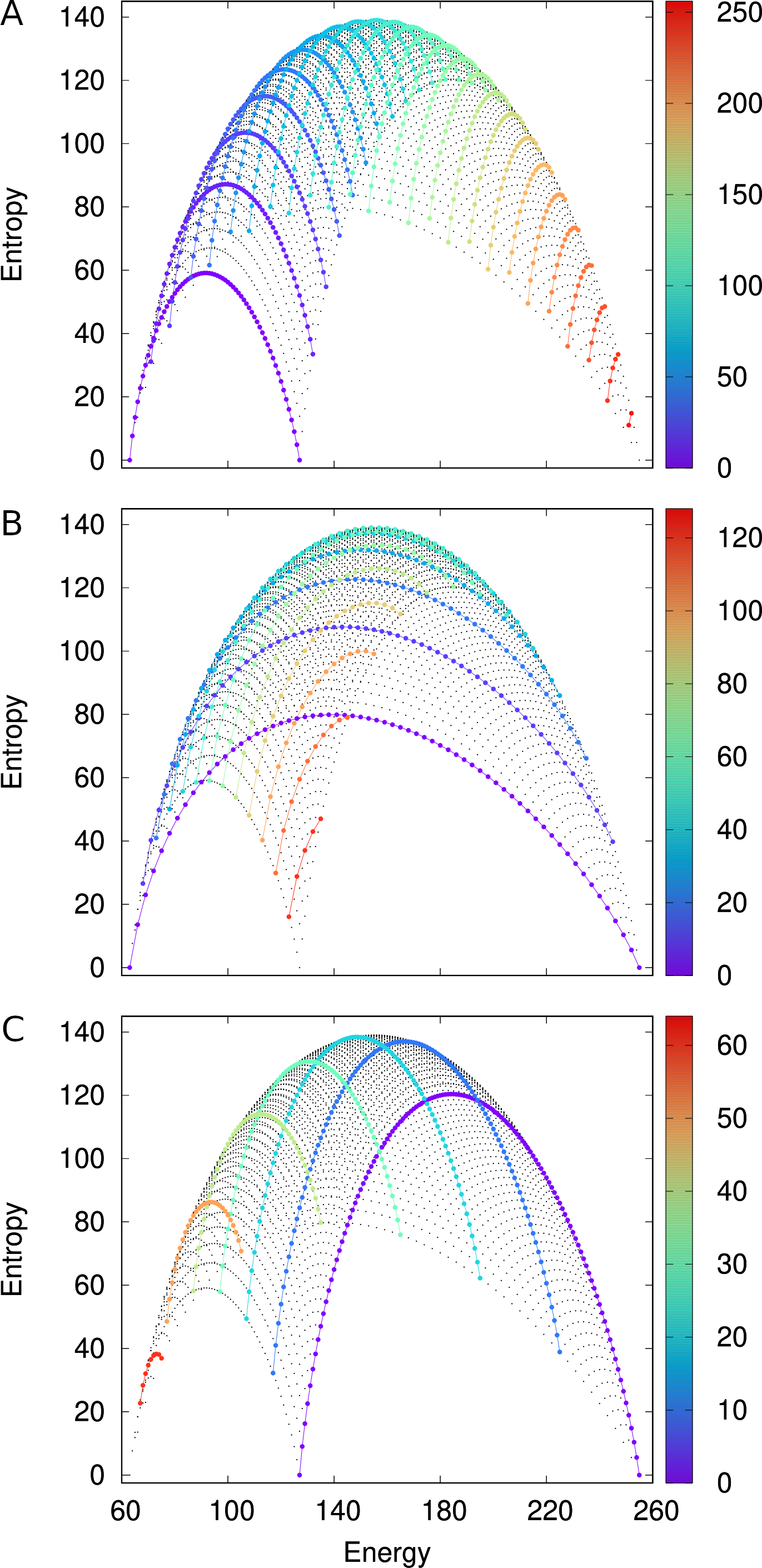
Figure 1: Partitioning the configuration space for $m=1$, $n=256$. Each panel shows a different partition of all $4\,225$ configurations (dots), each represented by its energy $E$ and entropy $S_{\mathrm{nd}}$. A set in a partition is shown as a color-coded thread of enlarged dots and corresponds to a fixed value of $n_{1}$ (A), $n_{2}$ (B), or $n_{4}$ (C). A thread’s color is picked from the panel’s color bar on the right for that fixed value. To avoid cluttering, only sets corresponding to multiple-of-$10$ values of $n_{1}$ are shown in panel A, and likewise for $n_{2}$ in panel B and $n_{4}$ in panel C. $E_{\mathrm{min}}^{1\times 256}=63$, $E_{\mathrm{max}}^{1\times 256}=255$.

Analyzing the system from a configuration-centric perspective (i.e., by essentially ignoring the possible degeneracy of certain energy levels) amounts to regarding both entropy and temperature as functions of $n_{1},n_{2}$. That is,

$$S_{\mathrm{nd}}(n_{1},n_{2})=\ln k_{1n}(n_{1},n_{2})$$ (14)

and, using Eq. (8) with $\Gamma^{\prime}(w)=\Gamma(w)\psi_{0}(w)$,

$$T^{-1}_{\mathrm{nd}}(n_{1},n_{2}) =\left(\frac{\partial S_{\mathrm{nd}}}{\partial x}\frac{\partial x}{\partial E}+\frac{\partial S_{\mathrm{nd}}}{\partial y}\frac{\partial y}{\partial E}\right)\biggr{\rvert}_{\genfrac{}{}{0.0pt}{}{x=n_{1}}{y=n_{2}}}$$ (15)

$$=U(n_{1},n_{2}),$$ (16)

where

$$U(n_{1},n_{2})={} 2\psi_{0}(n_{1}+n_{2}+n_{4}+1)-{}$$ (17)

$$\frac{4}{3}\,\psi_{0}(n_{1}+1)-2\psi_{0}(n_{2}+1)+\frac{4}{3}\,\psi_{0}(n_{4}+1).$$

Table 1: Details of the set of configurations for $n=25$ and $n_{4}=1$.

$E$	$S_{\mathrm{nd}}$	$n_{1}$	$n_{2}$	$n_{4}$	$k_{1n}^{n_{4}=1}$	One of the $k_{1n}^{n_{4}=1}$ tilings
$11$	$4.88$	$1$	$10$	$1$	$132$
$12$	$7.95$	$3$	$9$	$1$	$2\,860$
$13$	$9.79$	$5$	$8$	$1$	$18\,018$
$14$	$10.84$	$7$	$7$	$1$	$51\,480$
$15$	$11.29$	$9$	$6$	$1$	$80\,080$
$16$	$11.21$	$11$	$5$	$1$	$74\,256$
$17$	$10.66$	$13$	$4$	$1$	$42\,840$
$18$	$9.64$	$15$	$3$	$1$	$15\,504$
$19$	$8.13$	$17$	$2$	$1$	$3\,420$
$20$	$6.04$	$19$	$1$	$1$	$420$
$21$	$3.09$	$21$	$0$	$1$	$22$

Partitioning the configuration space can be achieved in this case by fixing the value of, say, $n_{1}$ and observing the configurations that result as $n_{2}$ and $n_{4}$ are varied. Taking $n=256$, for example, results in the $4\,225$ configurations shown as background dots in the $E\times S_{\mathrm{nd}}$ plots of Fig. 1. Each of panels A, B, C in the figure corresponds to a different partition of the configuration space, showing some of the sets that result from assigning fixed values to $n_{1}$, $n_{2}$, $n_{4}$, respectively. Each set can be seen to be generally characterized by a “smooth” succession of points along which the values of energy $E$ increase while the values of entropy $S_{\mathrm{sd}}$ first rise then decline. For a more manageable value of $n$ ($n=25$), we give all details of the $n_{4}=1$ set in Table 1, where $k_{1n}^{n_{4}=1}=k_{1n}\bigr{\rvert}_{n_{4}=1}$, including an illustration of one of the $k_{1n}^{n_{4}=1}$ tilings for each pair $n_{1},n_{2}$ of values. Clearly, the set in question is characterized by an initial preponderance of dominoes that, along the sequence of increasing values of $E$, eventually turns into a preponderance of squares.

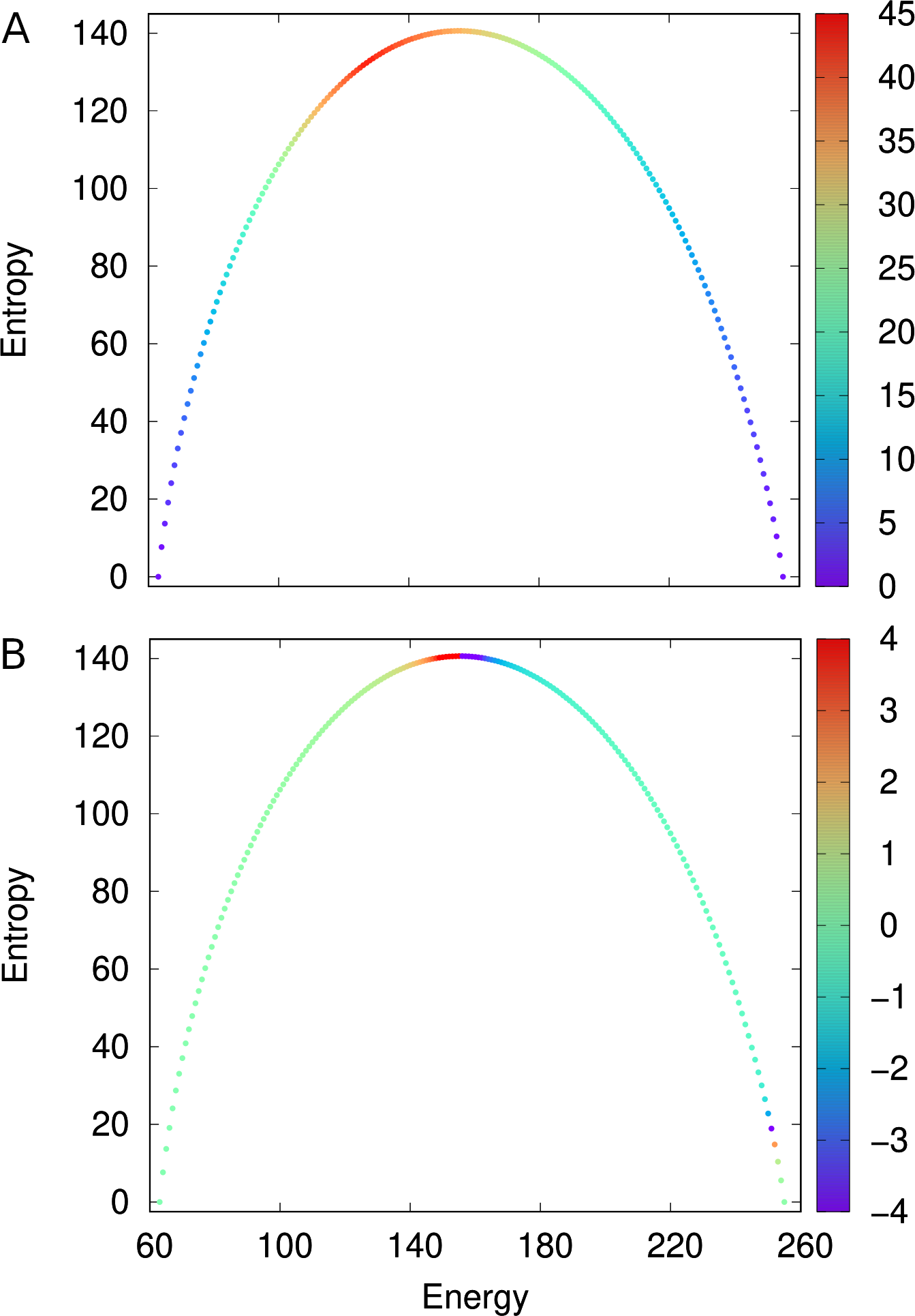
Figure 2: Entropy $S_{\mathrm{d}}$ as a function of energy $E$ for $m=1$, $n=256$. Dots are color-coded according to each panel’s color bar on the right to indicate the number of configurations (A) and the temperature $T_{\mathrm{d}}$ (B) for each energy level. For readability, the color bar in (B) leaves out $7$ points for which $T_{\mathrm{d}}<-4$ and $6$ others for which $T_{\mathrm{d}}>4$. These points get colored with the color corresponding to $-4$ or to $4$, respectively. $E_{\mathrm{min}}^{1\times 256}=63$, $E_{\mathrm{max}}^{1\times 256}=255$.

III.2 The degenerate case

An alternative analysis strategy is to recognize the existence of degenerate energy levels and take it fully into account. For each value $\varepsilon$ in the interval from $E_{\mathrm{min}}^{1\times n}$ to $E_{\mathrm{max}}^{1\times n}$, the system’s entropy and temperature are functions of $\varepsilon$. Entropy is given by

$$S_{\mathrm{d}}(\varepsilon)=\ln K(\varepsilon),$$ (18)

where

$$K(\varepsilon)=\sum_{\genfrac{}{}{0.0pt}{}{n_{1},n_{2}}{E(n_{1},n_{2})=\varepsilon}}k_{1n}(n_{1},n_{2}),$$ (19)

and temperature is such that

$$T^{-1}_{\mathrm{d}}(\varepsilon) =\frac{\partial S_{\mathrm{d}}}{\partial x}\frac{\partial x}{\partial E}+\frac{\partial S_{\mathrm{d}}}{\partial y}\frac{\partial y}{\partial E}$$ (20)

$$=\frac{1}{K(\varepsilon)}\sum_{\genfrac{}{}{0.0pt}{}{n_{1},n_{2}}{E(n_{1},n_{2})=\varepsilon}}\left(\frac{\partial k_{1n}}{\partial x}\frac{\partial x}{\partial E}+\frac{\partial k_{1n}}{\partial y}\frac{\partial y}{\partial E}\right)\biggr{\rvert}_{\genfrac{}{}{0.0pt}{}{x=n_{1}}{y=n_{2}}}$$ (21)

$$=\sum_{\genfrac{}{}{0.0pt}{}{n_{1},n_{2}}{E(n_{1},n_{2})=\varepsilon}}\frac{k_{1n}(n_{1},n_{2})}{K(\varepsilon)}\,U(n_{1},n_{2}).$$ (22)

That is, $T^{-1}_{\mathrm{d}}(\varepsilon)$ is a convex combination of $U(n_{1},n_{2})$ for those configurations for which $E(n_{1},n_{2})=\varepsilon$.

Thus, as far as representing configurations by their $E$ and $S_{\mathrm{d}}$ values is concerned, all configurations for which the value of $E$ is the same become conjoined in an $E\times S_{\mathrm{d}}$ plot. This is illustrated in the panels of Fig. 2 for $n=256$. As expected, this figure’s panel A reveals a greater variety of configurations contributing to $S_{\mathrm{d}}$ near the midrange values of $E$. As for panel B, overall we also see $T_{\mathrm{d}}$ behave as expected, that is, slightly above zero and increasing before $S_{\mathrm{d}}$ peaks as $E$ grows, then abruptly negative and increasing toward slightly below zero. However, a closer examination reveals a sudden flip back to positive temperatures for the highest four values of $E$: for $E=252$ and only one of the two contributing configurations ($n_{1}=252,n_{2}=0,n_{4}=1$); for $E=253$ and the only contributing configuration ($n_{1}=252,n_{2}=2,n_{4}=0$); for $E=254$ and the only contributing configuration ($n_{1}=254,n_{2}=1,n_{4}=0$); and for $E=255$ and the only contributing configuration ($n_{1}=256,n_{2}=n_{4}=0$).

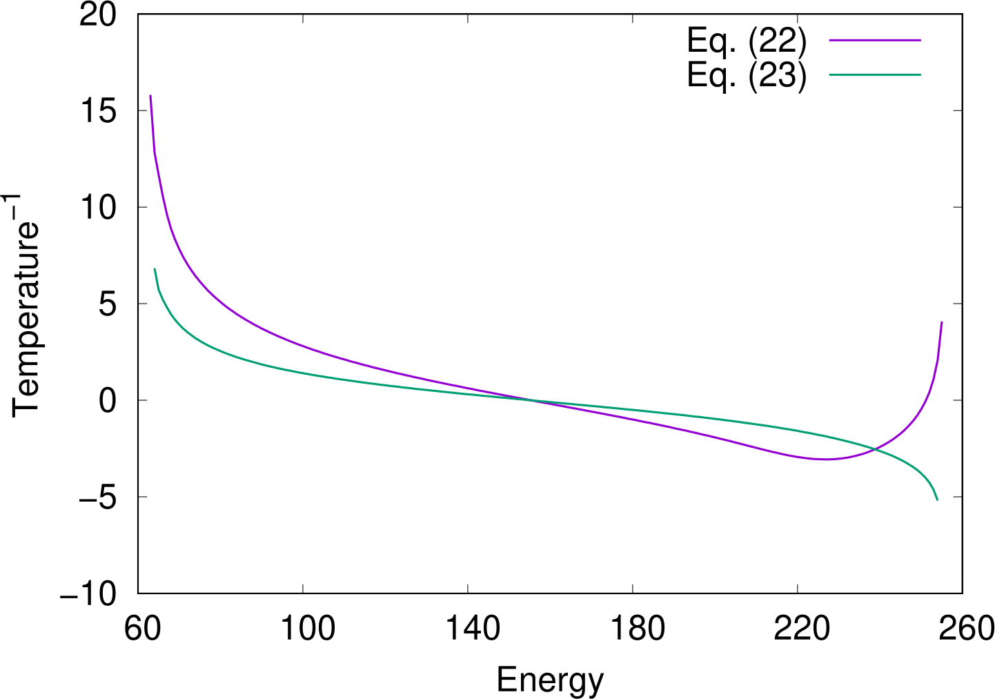
Figure 3: $T_{\mathrm{d}}^{-1}$ as a function of energy $E$ according to Eqs. (22) and (23).

This can be further explored as in Fig. 3, which illustrates the behavior of $T_{\mathrm{d}}^{-1}$ according to both Eq. (22) and

$$T_{\mathrm{d}}^{-1}(\varepsilon)\approx\frac{S_{\mathrm{d}}(\varepsilon+1)-S_{\mathrm{d}}(\varepsilon-1)}{2}.$$ (23)

The sudden turn to positive temperatures described above is clearly visible, as is the overall discrepancy between the two curves. We attribute these differences to the problems that are inherent to using $\Gamma^{\prime}$ to assess the local variability of the factorial function, as discussed in the introduction to Sec. III. In spite of these difficulties, for most of the energy spectrum Eq. (22) provides a reasonable representation of the actual quantity. It is also significant that the use of $\Gamma^{\prime}$ is the only available analytical technique for temperature assessment in the case at hand.

III.3 Remarks on computational tractability

In terms of the computational difficulties involved, an important point to note if we were to move beyond $n=256$ is that obtaining plots like the ones in Figs. 1 and 2 would become increasingly harder. This is so because those plots contemplate all possible configurations of the system, which for $n=1,2,\ldots,2^{15}$ grows from $1$ to $67\,125\,249$, as shown in Fig. 4. These numbers are not particularly impressive, but already for $n=2^{16}$ we found that $128$ GB of memory were insufficient for the Mathematica 13 system to generate all configurations. (Regarding notation, in the caption of Fig. 4, and henceforth, we use the Iverson bracket $[P]$ for $P$ a logical proposition. $[P]$ equals $1$ if $P$ is true, $0$ if $P$ is false. This notation generalizes the Kronecker delta, since $[i=j]=\delta_{ij}$.)

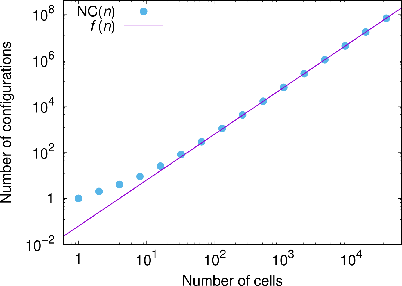
Figure 4: Total number of configurations, for $m=1$, as the function $\mathrm{NC}(n)$ of the number of cells $n$. The power law that fits the points asymptotically is $f(n)=4^{-2}n^{2}$. This comes from $\mathrm{NC}(n)=\sum_{n_{1}=0}^{n}\sum_{n_{2}=0}^{\lfloor(n-n_{1})/2\rfloor}[(n-n_{1}-2n_{2})\bmod 4=0]\approx\sum_{n_{1}=0}^{n}\sum_{n_{2}=0}^{\lfloor(n-n_{1})/2\rfloor}4^{-1}$, which equals $4^{-2}(n+1)(n+3)$ if $n$ is odd, $4^{-2}(n+2)^{2}$ if $n$ is even. Either of these expressions tends asymptotically to $f(n)$. Counting each configuration as only $4^{-1}$ targets the many situations where the condition $(n-n_{1}-2n_{2})\bmod 4=0$ fails, causing three out of four configurations to be invalid.

On the other hand, it must be kept in mind that Figs. 1 and 2 could only be obtained due to the availability of the closed-form expression for $k_{1n}$ given in Eq. (8), which essentially does away with the need to count the number of tilings admitted by each of the configurations in order to calculate entropy. Totaling this number over all configurations results in $\sum_{\varepsilon}K(\varepsilon)$, whose growth as a function of $n$ is depicted in Fig. 5. Crucially, for $n=256$ the value of $\sum_{\varepsilon}K(\varepsilon)$ is already of the order of $10^{63}$, which can be expected to be surpassed by many orders of magnitude as we consider the $m>1$ cases even for boards with a similar number of cells. Nothing like Eq. (8) is known for $m>1$, so clearly generalizing the special case of $m=1$ requires the ability to estimate entropy without counting the number of tilings admitted by any given configuration.

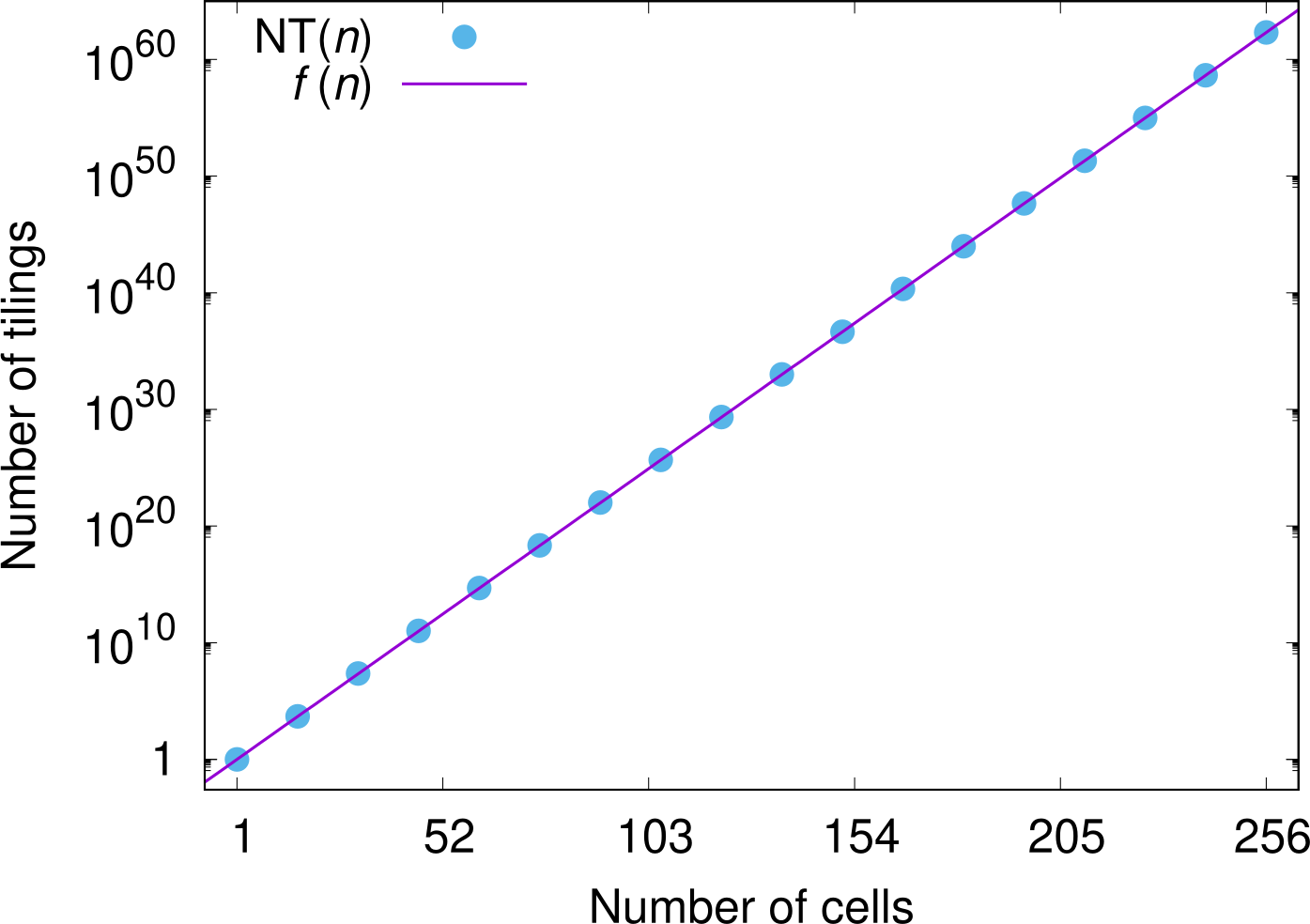
Figure 5: Total number of tilings, for $m=1$, as the function $\mathrm{NT}(n)=\sum_{\varepsilon}K(\varepsilon)$ of the number of cells $n$. The exponential fitting the points is $f(n)=e^{0.562663(n-1)}$.

IV The general case

For the general case we follow the same two strategies used in Sec. III, i.e., we study both the nondegenerate case (by focusing on individual configurations even though in general there can be several of them for the same energy level) and the degenerate one. As previously, therefore, the first strategy essentially sidelines the issue of energy-level degeneracy, thus allowing some partitions of the configuration space to be highlighted as in Fig. 1. Our approach relies on sampling tilings randomly, calculating the energy level for each sample, then adding some contribution to the ongoing entropy estimate for that energy level.

IV.1 Entropy estimation

Our approach to obtain entropy estimates is to use the Wang-Landau method [35, 36], which is a Monte Carlo Markov Chain (MCMC) method with well-established convergence properties [40, 41] to estimate state densities in statistical models. MCMC methods work by placing a walker at some randomly chosen initial state and then having it hop from state to state according to the chain’s transition probabilities, recording information along the way until some stopping criterion is met. The specific formulation we use is derived from the Metropolis-Hastings method [42, 43], in which the transition probabilities are based on the chain’s detailed-balance conditions and therefore make the desired stationary distribution explicit. Upon convergence to all detailed-balance conditions being satisfied, that is the distribution that will be observed (see Sec. IV.2).

Given the values of $m$ and $n$, the state space in this study is the set of all tilings of the $m\times n$ board by squares, dominoes, and tetraminoes. Each tiling is relative to a configuration unequivocally specified by the values of $n_{1}$ and $n_{2}$. A tiling’s target probability in the desired stationary distribution is proportional to $k_{mn}^{-1}(n_{1},n_{2})$, whose value is unknown but can be estimated, once an estimate $\hat{S}(n_{1},n_{2})$ is available for the corresponding configuration’s entropy $S(n_{1},n_{2})$, as $e^{-\hat{S}(n_{1},n_{2})}$. Thus, given two tilings $t$ and $t^{\prime}\neq t$, of configurations $n_{1},n_{2}$ and $n^{\prime}_{1},n^{\prime}_{2}$, respectively, the detailed-balance condition for them reads

$$e^{-\hat{S}(n_{1},n_{2})}g_{t\to t^{\prime}}a_{t\to t^{\prime}}=e^{-\hat{S}(n^{\prime}_{1},n^{\prime}_{2})}g_{t^{\prime}\to t}a_{t^{\prime}\to t},$$ (24)

where $g_{t\to t^{\prime}}a_{t\to t^{\prime}}$ is the transition probability from $t$ to $t^{\prime}$, broken down into the probability $g_{t\to t^{\prime}}$ that tiling $t^{\prime}$ is generated as a possible successor to tiling $t$ and the probability $a_{t\to t^{\prime}}$ of actually accepting the succession.

Given $g_{t\to t^{\prime}}$ and $g_{t^{\prime}\to t}$, the acceptance probability of $t^{\prime}$ given $t$ is defined as

$$a_{t\to t^{\prime}}=\min\left\{1,\frac{e^{-\hat{S}(n^{\prime}_{1},n^{\prime}_{2})}g_{t^{\prime}\to t}}{e^{-\hat{S}(n_{1},n_{2})}g_{t\to t^{\prime}}}\right\},$$ (25)

whence it follows that

$$\frac{a_{t\to t^{\prime}}}{a_{t^{\prime}\to t}}=\frac{e^{-\hat{S}(n^{\prime}_{1},n^{\prime}_{2})}g_{t^{\prime}\to t}}{e^{-\hat{S}(n_{1},n_{2})}g_{t\to t^{\prime}}}.$$ (26)

The definition in Eq. (25), therefore, leads directly to the condition in Eq. (24).

IV.2 Successor generation

We assume $g_{t\to t^{\prime}}>0$ if and only if $t^{\prime}$ can be obtained from $t$ either through the split of one tile (a domino or a tetramino) into two tiles (two squares or two dominoes, respectively) or through the merger of two tiles (two adjacent squares or two longitudinally adjacent dominoes) into one single tile (a domino or a tetramino, respectively). If $g_{t\to t^{\prime}}>0$ does indeed hold, then so does $g_{t^{\prime}\to t}>0$. It follows that the Markov chain in question is ergodic, that is, both aperiodic (since $\sum_{t^{\prime}}g_{t\to t^{\prime}}a_{t\to t^{\prime}}<1$, as there is always the possibility of rejection [44], so whenever transitioning from $t$ it is possible to remain at $t$) and irreducible (i.e., any state can be reached from any other). Therefore, the chain has a unique stationary distribution, which as discussed in Sec. IV.1 is proportional to $e^{-\hat{S}}$.

Let $n^{t}_{\mathrm{s}}$ be the number of dominoes or tetraminoes in tiling $t$, and $n^{t}_{\mathrm{m}}$ the number of pairs of adjacent squares or pairs of longitudinally adjacent dominoes in $t$. The generation of $t^{\prime}$ from $t$ starts with deciding which operation, the split of a domino into two squares or a tetramino into two dominoes (with probability $p^{t}_{\mathrm{s}}$) or the merger of two adjacent squares or two longitudinally adjacent dominoes (with probability $p^{t}_{\mathrm{m}}=1-p^{t}_{\mathrm{s}}$), is to be applied. Probability $p^{t}_{\mathrm{s}}$ is given by

$$p^{t}_{\mathrm{s}}=\frac{[n^{t}_{\mathrm{s}}>0]}{[n^{t}_{\mathrm{s}}>0]+[n^{t}_{\mathrm{m}}>0]},$$ (27)

so $p^{t}_{\mathrm{s}}$ equals $0$, $2^{-1}$, or $1$, since $n^{t}_{\mathrm{s}}+n^{t}_{\mathrm{m}}>0$ always holds. Once the decision of whether to split or to merge has been made, the tile to be split or the pair of tiles to be merged is chosen uniformly at random. We then have

$$g_{t\to t^{\prime}}=\begin{cases}(n^{t}_{\mathrm{s}})^{-1}&\text{ if }t^{\prime}\in T_{\mathrm{s}}^{t}\text{ and }n_{\mathrm{m}}^{t}=0,\\ (n^{t}_{\mathrm{m}})^{-1}&\text{ if }t^{\prime}\in T_{\mathrm{m}}^{t}\text{ and }n_{\mathrm{s}}^{t}=0,\\ (2n^{t}_{\mathrm{s}})^{-1}&\text{ if }t^{\prime}\in T_{\mathrm{s}}^{t}\text{ and }n_{\mathrm{s}}^{t}n_{\mathrm{m}}^{t}>0,\\ (2n^{t}_{\mathrm{m}})^{-1}&\text{ if }t^{\prime}\in T_{\mathrm{m}}^{t}\text{ and }n_{\mathrm{s}}^{t}n_{\mathrm{m}}^{t}>0,\\ 0&\text{ if }t^{\prime}\notin T_{\mathrm{s}}^{t}\cup T_{\mathrm{m}}^{t}.\end{cases}$$ (28)

In this equation, $T_{\mathrm{s}}^{t}$ comprises the $n_{\mathrm{s}}^{t}$ tilings obtainable from $t$ via a split and $T_{\mathrm{m}}^{t}$ comprises the $n_{\mathrm{m}}^{t}$ tilings obtainable from $t$ via a merger.

IV.3 Implementation of the Wang-Landau method

Our implementation of the Wang-Landau method follows the steps outlined next, where $\mathrm{hist}_{E}$ and $\mathrm{hist}_{\hat{S}}$ are histograms to record how many times each energy level is observed during the walker’s traversal of the Markov chain and this level’s entropy estimate, respectively. A parameter $f$ is used to control the entropy estimates. It is set to $1$ initially and is decreased to half its current value at each reset of $\mathrm{hist}_{E}$. Termination occurs when $f<10^{-10}$.

1. $t\leftarrow t_{0}$, where $t_{0}$ is a randomly chosen tiling;
   Let $\varepsilon_{t}$ be the energy level of $t$;

2. $\mathrm{hist}_{E}(\varepsilon)\leftarrow 0$ for every applicable energy level $\varepsilon$;
   $\mathrm{hist}_{\hat{S}}(\varepsilon)\leftarrow 0$ for every applicable energy level $\varepsilon$;
   $f\leftarrow 1$;
   $\mathrm{hist}_{E}(\varepsilon_{t})\leftarrow 1$;
   $\mathrm{hist}_{\hat{S}}(\varepsilon_{t})\leftarrow f$;
   Go to Step 4;

3. $\mathrm{hist}_{E}(\varepsilon)\leftarrow 0$ for every applicable energy level $\varepsilon$;

4. Generate a tentative successor $t^{\prime}$ of $t$;
   With probability $a_{t\to t^{\prime}}$, do $t\leftarrow t^{\prime}$;
   Let $\varepsilon_{t}$ be the energy level of $t$;
   If $\mathrm{hist}_{E}(\varepsilon_{t})=0$, go to Step 2;
   $\mathrm{hist}_{E}(\varepsilon_{t})\leftarrow\mathrm{hist}_{E}(\varepsilon_{t})+1$;
   $\mathrm{hist}_{\hat{S}}(\varepsilon_{t})\leftarrow\mathrm{hist}_{\hat{S}}(\varepsilon_{t})+f$;
   If $\mathrm{hist}_{E}$ is flat, do $f\leftarrow 2^{-1}f$ and go to Step 3;
   If $f\geq 10^{-10}$, repeat Step 4;

The random walk starts at the randomly chosen tiling $t_{0}$ and is restarted whenever an energy level not yet encountered is found. Both initially and when a restart occurs, the two histograms $\mathrm{hist}_{E}$ and $\mathrm{hist}_{\hat{S}}$ are reset in Step 2. Another opportunity for a reset, albeit a partial one, occurs when $\mathrm{hist}_{E}$ becomes flat and is then reset in Step 3. Flatness is detected in Step 4 whenever every energy level $\varepsilon$ encountered thus far has $\mathrm{hist}_{E}(\varepsilon)$ no lower than $95\%$ of the histogram’s average. Except for the resets in Steps 2 and 3, Step 4 keeps repeating until termination occurs. After this, for each energy level $\varepsilon$ reached by the walker the entropy estimate is relativized to that of energy level $\varepsilon^{*}=\arg\min_{\varepsilon^{\prime}}\mathrm{hist}_{\hat{S}}(\varepsilon^{\prime})$, via $\mathrm{hist}_{\hat{S}}(\varepsilon)\leftarrow\mathrm{hist}_{\hat{S}}(\varepsilon)-\mathrm{hist}_{\hat{S}}(\varepsilon^{*})$. In a run that reaches every energy level, $\varepsilon^{*}$ corresponds to the configuration $n_{1}=mn,n_{2}=0$, that is, $\varepsilon^{*}=2mn-m-n$ and $k_{mn}(n_{1},n_{2})=1$. In this case, the $\mathrm{hist}_{\hat{S}}(\varepsilon^{*})=0$ resulting from relativization is no longer an estimate but the exact value. Note that this holds automatically in the $m=1$ case of Sec. III.

IV.4 Handling degeneracy

As we normally do when handling the degenerate case, so too in the nondegenerate case we would like to associate an entropy estimate to each energy level directly. However, in general an energy level does not unequivocally determine a system configuration, so we opt instead to slightly alter the counting of squares and dominoes in a tiling. This is done by letting squares be counted in units of weight $1+\delta_{1}$ and dominoes in units of weight $1+\delta_{2}$. The values of $\delta_{1},\delta_{2}$ must be sufficiently small to not affect the value of $E$ in any meaningful way, while allowing any two distinct configurations that would otherwise have the same value of $E$ to be told apart from each other by the now slightly different values of $E$.

In practice, this amounts to substituting $n_{1}(1+\delta_{1})$ for $n_{1}$ in Eqs. (3) and (4), and likewise $n_{2}(1+\delta_{2})$ for $n_{2}$. From those two equations it follows that, to fulfill the purpose of identifying distinct configurations having the same value of $E$, we must have

$$3(n_{1}-n^{\prime}_{1})(1+\delta_{1})\neq 2(n^{\prime}_{2}-n_{2})(1+\delta_{2})$$ (29)

for all possible configurations $n_{1},n_{2}$ and $n^{\prime}_{1},n^{\prime}_{2}$ with $n_{1}\neq n^{\prime}_{1}$ or $n_{2}\neq n^{\prime}_{2}$. We use two randomly generated numbers of the order of $10^{-7}$, viz., $\delta_{1}=7.72453\times 10^{-7}$ and $\delta_{2}=1.47577\times 10^{-7}$, which makes it impossible for the condition in Eq. (29) to be violated. Note that counting tiles in this slightly warped manner can be used directly in the nondegenerate case, by letting

$$\hat{S}_{\mathrm{nd}}(n_{1},n_{2})=\mathrm{hist}_{\hat{S}}(\varepsilon),$$ (30)

where $\varepsilon$ is the energy level of configuration $n_{1},n_{2}$. It can also be used in the degenerate case, by coalescing together all energy levels having the same integral part. If $\mathcal{E}(\bar{\varepsilon})$ is the set of all energy levels sharing the same integral part $\bar{\varepsilon}$, then coalescing means letting

$$\hat{S}_{\mathrm{d}}(\bar{\varepsilon})=\ln\hat{K}(\bar{\varepsilon}),$$ (31)

where

$$\hat{K}(\bar{\varepsilon})=\sum_{\varepsilon^{\prime}\in\mathcal{E}(\bar{\varepsilon})}e^{\mathrm{hist}_{\hat{S}}(\varepsilon^{\prime})}.$$ (32)

This quantity is the counterpart, for when analytical treatment is not possible, of the $K(\varepsilon)$ defined in Eq. (19).

IV.5 The $\bm{m}\bm{=}\bm{4}$ and $\bm{m}\bm{=}\bm{n}$ cases

In Secs.IV.6 and IV.7, we give results of the Wang-Landau method for $4\times n$ and $n\times n$ boards. As previously, the possible values of $E$ in Eq. (3), now considering only their integral parts, range from a minimum that uses as many tetraminoes as possible, plus as few dominoes and squares as possible, to a maximum that uses squares exclusively.

For a $4\times n$ board, this minimum occurs for configuration $n_{1}=n_{2}=0,n_{4}=n$ and equals

$$E_{\mathrm{min}}^{4\times n}=4(n-1).$$ (33)

The maximum occurs for configuration $n_{1}=4n,n_{2}=n_{4}=0$ and equals

$$E_{\mathrm{max}}^{4\times n}=7n-4.$$ (34)

As for an $n\times n$ board, first let $a=n\bmod 4$. The minimum integral part of an energy level can be seen to occur for configuration $n_{1}=a^{2}\bmod 2,n_{2}=\lfloor a^{2}/2\rfloor,n_{4}=\lfloor n/4\rfloor(n+a)$, which yields

$$E_{\mathrm{min}}^{n\times n}={} 2(a^{2}-2\lfloor a^{2}/2\rfloor)+3\lfloor a^{2}/2\rfloor+{}$$ (35)

$$5\lfloor n/4\rfloor(n+a)-2n$$

$$={} 2a^{2}-\lfloor a^{2}/2\rfloor+5\lfloor n/4\rfloor(n+a)-2n.$$ (36)

The maximum, in turn, occurs for configuration $n_{1}=n^{2},n_{2}=n_{4}=0$, yielding

$$E_{\mathrm{max}}^{n\times n}=2n(n-1).$$ (37)

Our computational experiments on $4\times n$ and $n\times n$ boards were planned so that a board’s number of cells would not exceed $256$, as in Sec. III. Whenever the number of cells in use happens to be both a perfect square and a multiple of $16$ (as is $256$), a curious property, using $n_{\mathrm{cells}}$ to denote the number of cells, is that

$$\frac{3n_{\mathrm{cells}}}{4} =E_{\mathrm{max}}^{1\times n_{\mathrm{cells}}}-E_{\mathrm{min}}^{1\times n_{\mathrm{cells}}}$$ (38)

$$=E_{\mathrm{max}}^{4\times\frac{n_{\mathrm{cells}}}{4}}-E_{\mathrm{min}}^{4\times\frac{n_{\mathrm{cells}}}{4}}$$ (39)

$$=E_{\mathrm{max}}^{\sqrt{n_{\mathrm{cells}}}\times\sqrt{n_{\mathrm{cells}}}}-E_{\mathrm{min}}^{\sqrt{n_{\mathrm{cells}}}\times\sqrt{n_{\mathrm{cells}}}}.$$ (40)

That is, the size of the energy spectrum is the same in all three cases. Also, and not surprisingly, the configurations for which the minimum and maximum value of $E$ are obtained are the same in all three cases: $n_{1}=0,n_{2}=0,n_{4}=4^{-1}n_{\mathrm{cells}}$ for the minimum, $n_{1}=n_{\mathrm{cells}},n_{2}=n_{4}=0$ for the maximum.

Fixing $n_{\mathrm{cells}}$ at $256$ reveals further similarities. Not only are the two configurations of minimum and maximum energy the same in all three cases, but the set of $4\,225$ configurations of the $1\times 256$ case is the set of configurations of the $4\times 64$ and $16\times 16$ cases as well. To see that this is indeed the case, first consider that any configuration of either the $4\times 64$ or the $16\times 16$ case is also a configuration of the $1\times 256$ case (simply arrange the tiles in the $1\times 256$ board arbitrarily). Conversely, given that both $m$ and $n$ are multiples of $4$ in the $4\times 64$ and $16\times 16$ cases, then any configuration of the $1\times 256$ case is also a configuration of both the $4\times 64$ and $16\times 16$ cases. This too is seen to be straightforward, e.g.: first arrange the $n_{4}$ tetraminoes in columns of at most $m/4$ tiles each, then fill the remaining (partially filled or empty) columns with the $n_{2}$ dominoes and the $n_{1}$ squares.

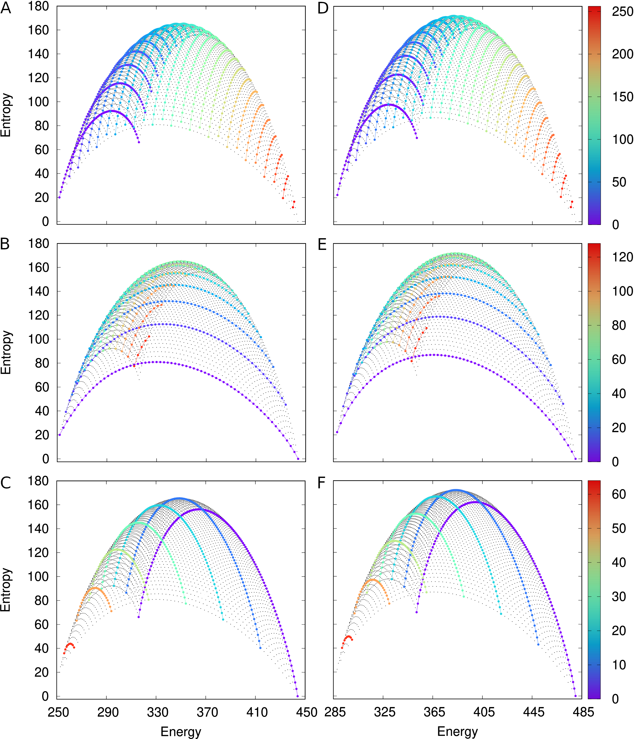
Figure 6: As in Fig. 1, now for two cases of $m>1$ with $n_{\mathrm{cells}}=256$, each configuration represented by its energy $E$ and entropy $\hat{S}_{\mathrm{nd}}$. (A–C) $m=4$, $n=64$, $E_{\mathrm{min}}^{4\times 64}=252$, $E_{\mathrm{max}}^{4\times 64}=444$; (D–F) $n=m=16$, $E_{\mathrm{min}}^{16\times 16}=288$, $E_{\mathrm{max}}^{16\times 16}=480$. Color codes refer to multiple-of-$10$ values of $n_{1}$ (A, D), $n_{2}$ (B, E), or $n_{4}$ (C, F).

These further similarities between the $1\times 256$, $4\times 64$, and $16\times 16$ cases are important because they allow us to check the results output by the Wang-Landau method on the $4\times 64$ and $16\times 16$ boards against those we already validated analytically for the $1\times 256$ board. The only differences we expect are significantly higher numbers of tilings, i.e., higher entropies and the corresponding adjustments in temperature. All else is expected to remain unaltered.

IV.6 The nondegenerate case

Our results from the Wang-Landau method on the $4\times 64$ and $16\times 16$ boards, when degeneracy is disregarded so that partitions of the configuration space can be observed, are summarized in the panels of Fig. 6. Each panel has exactly $4\,225$ background dots, one for each configuration, indicating that the MCMC walker reached all of them. The likeness of the set of panels corresponding to the $4\times 64$ board (A–C), or of those corresponding to the $16\times 16$ board (D–F), to Fig. 1 cannot be missed. In fact, as expected, only the entropy values help distinguish one case from the other two. While for the $1\times 256$ board we have $S_{\mathrm{nd}}<140$, for the $4\times 64$ and $16\times 16$ boards we have $\hat{S}_{\mathrm{nd}}<166$ and $\hat{S}_{\mathrm{nd}}<173$, respectively.

IV.7 The degenerate case

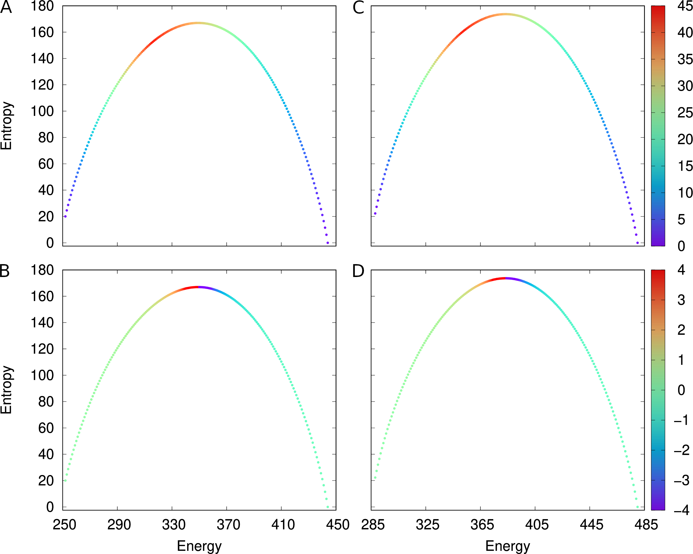
Figure 7: As in Fig. 2, now showing entropy $\hat{S}_{\mathrm{d}}$ as a function of energy $E$ for two cases of $m>1$ with $n_{\mathrm{cells}}=256$. (A, B) $m=4$, $n=64$, $E_{\mathrm{min}}^{4\times 64}=252$, $E_{\mathrm{max}}^{4\times 64}=444$; (C, D) $m=n=16$, $E_{\mathrm{min}}^{16\times 16}=288$, $E_{\mathrm{max}}^{16\times 16}=480$. Color codes refer to numbers of configurations (A, C) or to temperature $\hat{T}_{\mathrm{d}}$ (B, D).

When degeneracy is taken into account and all configurations for the same energy level are coalesced together, using the Wang-Landau method on the $4\times 64$ and $16\times 16$ boards yields the results shown in Fig. 7. This figure has two panels for the $4\times 64$ board (A, B) and two for the $16\times 16$ board (C, D). Two of the panels highlight the number of configurations contributing to each entropy value (A, C) and two others highlight the corresponding temperature (B, D). Temperature is now estimated from entropy differences, based on substituting the $\hat{S}_{\mathrm{d}}$ of Eq. (31) for $S_{\mathrm{d}}$ in Eq. (23). This results in

$$\hat{T}_{\mathrm{d}}^{-1}(\bar{\varepsilon})\approx\frac{\hat{S}_{\mathrm{d}}(\bar{\varepsilon}+1)-\hat{S}_{\mathrm{d}}(\bar{\varepsilon}-1)}{2}$$ (41)

for the combined energy levels of integral part $\bar{\varepsilon}$.

Once again, the resemblance of all four plots to the corresponding ones in Fig. 2 is hard to miss. Differences do exist, however, the clearest one relating to the maximum entropy levels in each case, as noted in Sec. IV.6. The other difference has to do with the temperature estimates, which in all three cases are color-coded in the lower panels, but are nevertheless hard to discern visually.

IV.8 Further remarks on computational tractability

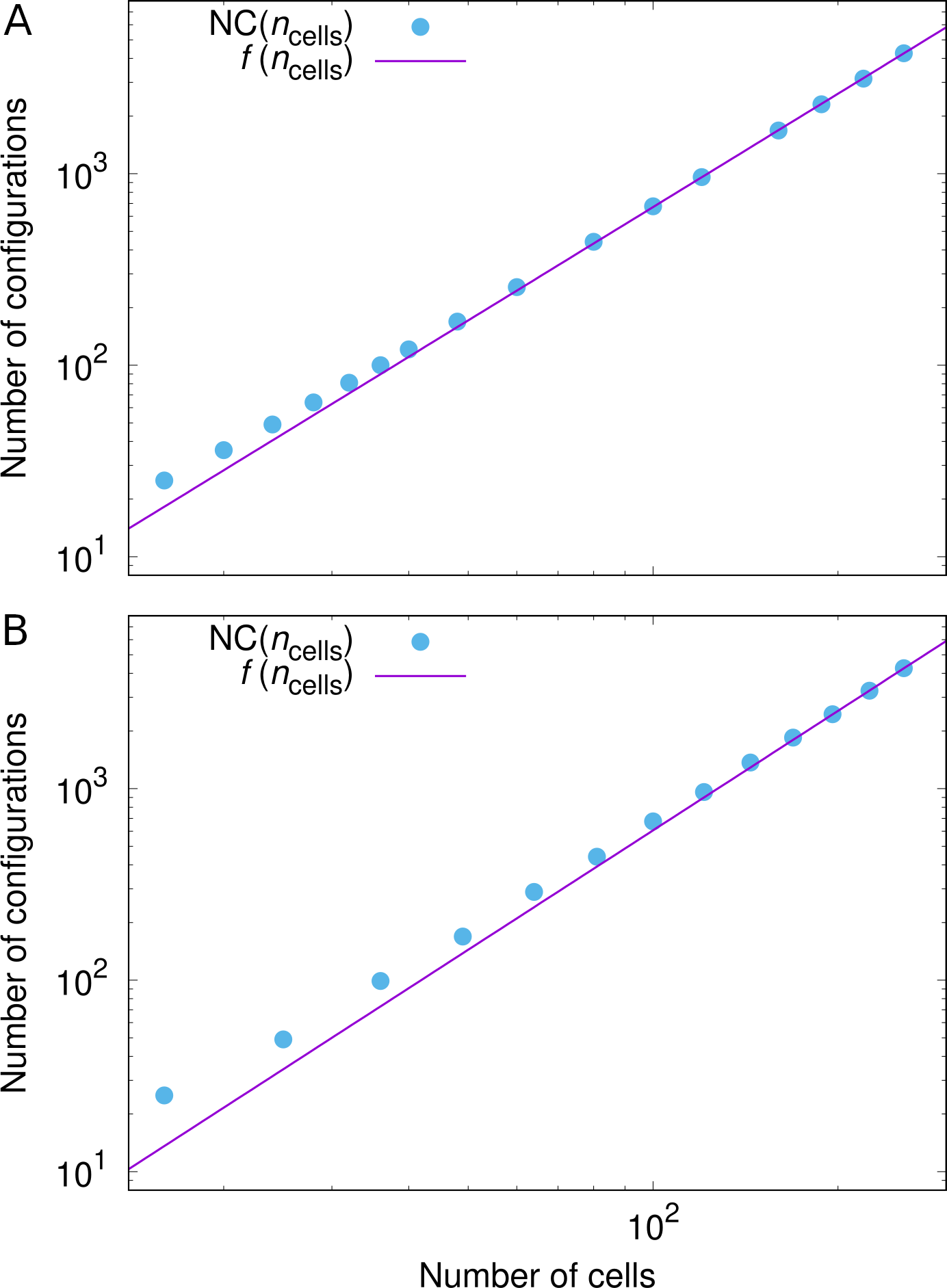
Figure 8: As in Fig. 4, now as the function $\mathrm{NC}(n_{\mathrm{cells}})$ for two cases of $m>1$ with $n_{\mathrm{cells}}\leq 256$. (A) $m=4$, $n=4^{-1}n_{\mathrm{cells}}$; (B) $m=n=\sqrt{n_{\mathrm{cells}}}$. The power law that fits the points asymptotically is $f(n_{\mathrm{cells}})=12.79^{-1}n_{\mathrm{cells}}^{1.96648}$ (A) or $f(n_{\mathrm{cells}})=23^{-1}n_{\mathrm{cells}}^{2.07212}$ (B).

We finalize Sec. IV by returning to the theme of computational tractability raised in Sec. III.3 in the context of the $m=1$ special case, for which analytical treatment is possible. The concern in that case was centered on the total number of configurations. These had to be enumerated to exhaustion for use in the analyses, a process that we found out is severely limited as the number of cells in the board grows. The total number of tilings $k_{1n}$ for each configuration, from which entropy is calculated, was in that case reason for no concern in terms of computational tractability, since the availability of a closed-form expression for $k_{1n}$ was itself the one key factor enabling analytical treatment.

In the context of the $m>1$ cases we have been handling in Sec. IV, the main concern related to computational tractability is the growth of the tiling space through which the MCMC walker navigates to estimate entropy. This space grows unimaginably quickly with both the total number of configurations for the different energy levels and especially the total number of tilings admitted by those configurations. A larger tiling space requires more steps for the walker to be able to roam sufficiently far and wide for convergence to occur. Figures 8 and 9 illustrate the growth trends of the two quantities.

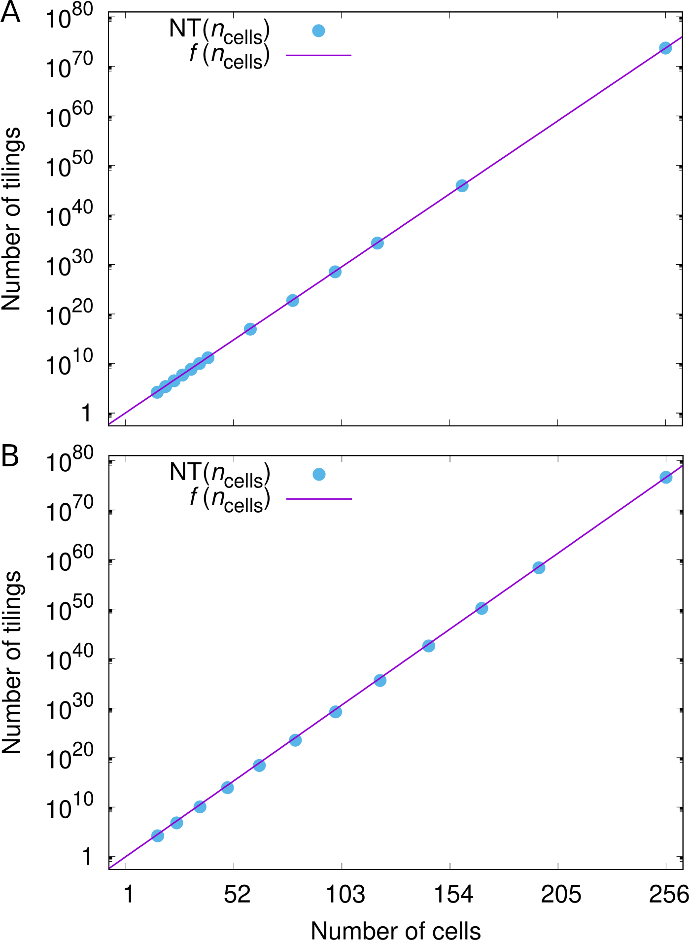
Figure 9: As in Fig. 5, now as the function $\mathrm{NT}(n_{\mathrm{cells}})=\sum_{\bar{\varepsilon}}\hat{K}(\bar{\varepsilon})$ for two cases of $m>1$ with $n_{\mathrm{cells}}\leq 256$. (A) $m=4$, $n=4^{-1}n_{\mathrm{cells}}$; (B) $m=n=\sqrt{n_{\mathrm{cells}}}$. The exponential that fits the points is $f(n_{\mathrm{cells}})=e^{0.665527(n_{\mathrm{cells}}-1)}$ (A) or $f(n_{\mathrm{cells}})=e^{0.691678(n_{\mathrm{cells}}-1)}$ (B).

Figure 8 is about the growth of the total number of configurations as $n_{\mathrm{cells}}$ grows. Panel A is for $4\times\frac{n_{\mathrm{cells}}}{4}$ boards, panel B for $\sqrt{n_{\mathrm{cells}}}\times\sqrt{n_{\mathrm{cells}}}$ boards. For each of these two cases we found the total number of configurations to asymptotically follow a power law similar to the quadratic one found for the $1\times n_{\mathrm{cells}}$ but still different from it. Figure 9, in turn, is about the growth of the total number of tilings as $n_{\mathrm{cells}}$ grows, with panels arranged analogously to Fig. 8. Exponentials in $n_{\mathrm{cells}}$ are still found, but now reaching significantly higher numbers. For $n_{\mathrm{cells}}=256$, a total number of tilings of the order of $10^{73}$ was found in the $4\times\frac{n_{\mathrm{cells}}}{4}$ case, of the order of $10^{76}$ in the $\sqrt{n_{\mathrm{cells}}}\times\sqrt{n_{\mathrm{cells}}}$ case. These are to be compared with the total number of tilings in the $1\times n_{\mathrm{cells}}$ case, which is of the order of $10^{63}$.

V Conclusion

The scientific interest in tilings of the plane, and sometimes of higher-dimensional regions as well, has a history that spans several centuries. In the last six to seven decades, however, it gained new momentum motivated by the realization in the early 20th century that some decision problems could be neither easy nor hard to solve, but simply undecidable. Though it soon turned out that undecidability was not an issue, interest did not wane. Instead, due to efforts by both mathematicians working on discrete systems and applied physicists in fields related to atomic- and molecular-scale phenomena, progress with important milestones was maintained. By and large, however, it seems fair to say that most key theoretical advancements, even those that inspired real-world applications, came from considering tilings of the whole, unbounded plane.

Studying tilings of bounded regions of the plane requires handling the combinatorics of finite discrete structures, a field in which exact closed-form expressions for counting quantities of interest are hard to come by. In this study, we considered rectangular regions of the plane and how to tile them with rectangular tiles. We concentrated on the tile-type set containing the square, the domino, and the straight tetramino. Simple though this system may seem, in the general case of an $m\times n$ board not even the number of configurations (how many squares, dominoes, tetraminoes) that are feasible can be counted exactly, not even indirectly via recurrence relations. Our approach has been to regard the system from the standpoint of their statistical properties and consider its configurations, states (tilings), energy, entropy, and temperature in such a way as to illuminate some of its inner workings. We followed two parallel tracks, one for the $m=1$ case, the other for more general, $m>1$ cases. Given our choice of a tile contact-based energy function, the $m=1$ case is fully tractable analytically. The other track relied on the Wang-Landau method for state-density estimation in the $m>1$ cases, and on the subsequent calculation of approximate entropies and temperatures. By alternately disregarding and taking into account the issue of energy-level degeneracy, we were able to demonstrate how to partition the configuration space and thereby highlight how the system’s configurations relate to one another, as well as to entropy and temperature.

A lot of room is left for methodological improvements. In particular, given the computationally intensive character of the Wang-Landau method, some of the techniques already developed for exploring the state space in parallel [45] should be considered. Additionally, our choice of energy function has been about the simplest imaginable. Considering the next level of sophistication, by adopting an energy function based on tile areas instead of simply perimeters, is bound to bring the entire approach closer to some of the applications that might benefit from it. Some of these applications are in areas such as modeling biological tissues [32, 34] and their properties [46, 47], and developing bioinspired metamaterials [48].