Feasible approximation of matching equilibria for large-scale matching for teams problems

Abstract.

We propose a numerical algorithm for computing approximately optimal solutions of the matching for teams problem. Our algorithm is efficient for problems involving a large number of agent categories and allows for the measures describing the agent types to be non-discrete. Specifically, we parametrize the so-called transfer functions and develop a parametric version of the dual formulation. Our algorithm tackles this parametric formulation and produces feasible and approximately optimal solutions for the primal and dual formulations of the matching for teams problem. These solutions also yield upper and lower bounds for the optimal value, and the difference between the upper and lower bounds provides a direct sub-optimality estimate of the computed solutions. Moreover, we are able to control a theoretical upper bound on the sub-optimality to be arbitrarily close to 0 under mild conditions. We subsequently prove that the approximate primal and dual solutions converge when the sub-optimality goes to 0 and their limits constitute a true matching equilibrium. Thus, the outputs of our algorithm are regarded as an approximate matching equilibrium. We also analyze the theoretical computational complexity of our parametric formulation as well as the sparsity of the resulting approximate matching equilibrium. Through numerical experiments, we showcase that the proposed algorithm can produce high-quality approximate matching equilibria and is applicable to versatile settings, including a high-dimensional setting involving 100 agent categories.

1. Introduction

The goal of this paper is to provide an algorithm which constructs approximately optimal solutions of the matching for teams problem in theoretical economics involving a large number of agent categories. The matching for teams problem was introduced by Carlier and Ekeland [22], and the setting is described as follows.

Assumption 1.1 (Matching for teams [22, Section 2.4]).

We make the following assumptions:

1. For $i=1,\ldots,N$ (where $N\in\mathbb{N}$), $(\mathcal{X}_{i},d_{\mathcal{X}_{i}})$ is a compact metric space (with metric $d_{\mathcal{X}_{i}}$) and ${\bm{\mathcal{X}}}:=\mathcal{X}_{1}\times\cdots\times\mathcal{X}_{N}$.

2. $(\mathcal{Z},d_{\mathcal{Z}})$ is a compact metric space.

3. For $i=1,\ldots,N$, $\mu_{i}\in\mathcal{P}(\mathcal{X}_{i})$ is a probability measure on $\mathcal{X}_{i}$.

4. For $i=1,\ldots,N$, $c_{i}:\mathcal{X}_{i}\times\mathcal{Z}\to\mathbb{R}$ is continuous.

Using the terminologies of Carlier and Ekeland [22], the matching for teams problem describes an economic game involving $N$ categories of agents (e.g., one category of consumer and $N-1$ categories of different producers), where the number of agents in each category is infinite. The spaces $\mathcal{X}_{1},\ldots,\mathcal{X}_{N}$, referred to as type spaces, each represents the types of agents from a category. The space $\mathcal{Z}$, referred to as the quality space, represents a type of indivisible good with various qualities. In category $i$, the distribution of agent types is characterized by the probability measure $\mu_{i}\in\mathcal{P}(\mathcal{X}_{i})$. Moreover, the function $c_{i}(x_{i},z)$ represents the cost for an agent with type $x_{i}\in\mathcal{X}_{i}$ to be matched to a unit of good with quality $z\in\mathcal{Z}$. In order for a unit of good with quality $z\in\mathcal{Z}$ to be traded, one agent from each category must come together to form a team and exchange money within the team. The goal is to find a matching equilibrium defined as follows.

Definition 1.2 (Matching equilibrium [22, Definition 1]).

Let Assumption 1.1 hold. A matching equilibrium consists of continuous functions $\varphi_{1},\ldots,\varphi_{N}:\mathcal{Z}\to\mathbb{R}$, probability measures $\gamma_{1},\ldots,\gamma_{N}\in\mathcal{P}(\mathcal{X}_{i}\times\mathcal{Z})$, and a probability measure $\nu\in\mathcal{P}(\mathcal{Z})$ such that:

1. for $i=1,\ldots,N$, $\gamma_{i}\in\Gamma(\mu_{i},\nu)$, where $\Gamma(\mu_{i},\nu)$ denotes the set of couplings of $\mu_{i}$ and $\nu$, i.e., $\Gamma(\mu_{i},\nu)$ contains all probability measures on $\mathcal{X}_{i}\times\mathcal{Z}$ whose marginals on $\mathcal{X}_{i}$ and $\mathcal{Z}$ are $\mu_{i}$ and $\nu$;

2. $\sum_{i=1}^{N}\varphi_{i}(z)=0$ for all $z\in\mathcal{Z}$;

3. for $i=1,\ldots,N$, $\varphi_{i}^{c_{i}}(x_{i})+\varphi_{i}(z)=c_{i}(x_{i},z)$ for $\gamma_{i}$-almost all $(x_{i},z)\in\mathcal{X}_{i}\times\mathcal{Z}$, where $\varphi_{i}^{c_{i}}:\mathcal{X}_{i}\to\mathbb{R}$ is called the $c_{i}$-transform of $\varphi_{i}$ and is defined by

   $$\varphi_{i}^{c_{i}}(x_{i}):=\inf_{z\in\mathcal{Z}}\big{\{}c_{i}(x_{i},z)-\varphi_{i}(z)\big{\}}\qquad\forall x_{i}\in\mathcal{X}_{i}.$$

In Definition 1.2, $\varphi_{i}(z)$ represents the amount of money received by an agent of category $i$ when trading a unit of good with quality $z\in\mathcal{Z}$, $\nu\in\mathcal{P}(\mathcal{Z})$ represents the distribution of the qualities of traded goods, and for $i=1,\ldots,N$, $\gamma_{i}\in\Gamma(\mu_{i},\nu)$ describes the matching between agents of category $i$ and different qualities of goods. The condition (ME1) ensures that every agent is matched to some good. The condition (ME2) is called the balance condition as it requires each team to be self-financed, e.g., all money paid by the consumers will be transferred to the producers. The condition (ME3) requires that an agent of type $x_{i}\in\mathcal{X}_{i}$ is matched to a unit of good with quality $z$ only if $z$ minimizes the net cost, i.e., $z\in\operatorname*{arg\,min}_{z^{\prime}\in\mathcal{Z}}\big{\{}c_{i}(x_{i},z^{\prime})-\varphi_{i}(z^{\prime})\big{\}}$. In the following, we present two examples of the matching for teams problem.

Example 1.3 (Application 1: equilibrium of business location distribution).

Let us consider the study of the geographic distribution of a type of business in a city by modeling the location of business outlets as well as the employees’ workplace choices as a game involving $N$ player populations. In this game, the first $N-1$ player populations represent $N-1$ categories of employees and the $N\text{-th}$ player population represents the business owners. Specifically, the set $\mathcal{Z}\subset\mathbb{R}^{2}$ represents the locations (in longitude and latitude) in the city where business outlets could possibly be located at. For $i=1,\ldots,N-1$, the set $\mathcal{X}_{i}\subset\mathbb{R}^{2}$ represents the locations in the city where the $i$-th category of employees can reside and $\mu_{i}\in\mathcal{P}(\mathcal{X}_{i})$ represents the distribution of the dwellings of the $i$-th category of employees. The set $\mathcal{X}_{N}$ represents the possible locations of the suppliers of the business in the city and $\mu_{N}\in\mathcal{P}(\mathcal{X}_{N})$ denotes their geographic distribution. Moreover, for $i=1,\ldots,N-1$, the cost function $c_{i}(\cdot,\;\cdot)$ represents the commuting cost of the $i$-th category of employees, i.e., $c_{i}({\bm{x}}_{i},{\bm{z}})$ denotes the cost of commuting from an employee’s home located at ${\bm{x}}_{i}\in\mathcal{X}_{i}$ to a business outlet located at ${\bm{z}}\in\mathcal{Z}$. Furthermore, the cost function $c_{N}:\mathcal{X}_{N}\times\mathcal{Z}\to\mathbb{R}$ represents the restocking cost of a business outlet, i.e., $c_{N}({\bm{x}}_{N},{\bm{z}})$ denotes the cost of transporting goods from a supplier at ${\bm{x}}_{N}\in\mathcal{X}_{N}$ to a business outlet located at ${\bm{z}}\in\mathcal{Z}$. Under this setting, we are interested in finding a matching equilibrium consisting of $(\varphi_{i}:\mathcal{Z}\to\mathbb{R})_{i=1:N}$, $\big{(}\gamma_{i}\in\mathcal{P}(\mathcal{X}_{i}\times\mathcal{Z})\big{)}_{i=1:N}$, and $\nu\in\mathcal{P}(\mathcal{Z})$. For $i=1,\ldots,N-1$, $\varphi_{i}({\bm{z}})$ denotes the amount of salary earned by an employee working at a business outlet located at ${\bm{z}}\in\mathcal{Z}$. $\varphi_{N}({\bm{z}})$ denotes the negative of the total amount of salary paid out by a business outlet located at ${\bm{z}}\in\mathcal{Z}$ to the $N-1$ categories of employees. $\nu\in\mathcal{P}(\mathcal{Z})$ describes the geographic distribution of the business outlets in the city and $\gamma_{N}\in\mathcal{P}(\mathcal{X}_{N}\times\mathcal{Z})$ describes how the business outlets choose the suppliers to restock from. Moreover, for $i=1,\ldots,N-1$, $\gamma_{i}\in\mathcal{P}(\mathcal{X}_{i}\times\mathcal{Z})$ describes where the employees in the $i$-th category choose to work at depending on where they reside. At equilibrium, the condition $\gamma_{i}\in\Gamma(\mu_{i},\nu)$ for $i=1,\ldots,N-1$ requires each employee to work at some business outlet, and the condition $\gamma_{N}\in\Gamma(\mu_{N},\nu)$ requires each supplier to be supplying some business outlet. The balance condition $\sum_{i=1}^{N}\varphi_{i}({\bm{z}})=0$ for all ${\bm{z}}\in\mathcal{Z}$ ensures that the total amount of salary paid out by each business owner, i.e., $-\varphi_{N}({\bm{z}})$, is equal to the total amount of salary received by the $N-1$ categories of employees, i.e., $\sum_{i=1}^{N-1}\varphi_{i}({\bm{z}})$. Finally, for $i=1,\ldots,N$, the condition $\varphi_{i}^{c_{i}}({\bm{x}}_{i})+\varphi_{i}({\bm{z}})=c_{i}({\bm{x}}_{i},{\bm{z}})$ for $\gamma_{i}$-almost all $({\bm{x}}_{i},{\bm{z}})\in\mathcal{X}_{i}\times\mathcal{Z}$ states that each employee acts rationally when choosing the workplace, i.e., an employee that resides at ${\bm{x}}_{i}$ minimizes the commuting cost $c_{i}({\bm{x}}_{i},{\bm{z}})$ minus the salary $\varphi_{i}({\bm{z}})$ when deciding the workplace, and each business owner acts rationally when choosing the location of the business outlet, i.e., a business owner with supplier at ${\bm{x}}_{N}$ minimizes the cost $c_{N}({\bm{x}}_{N},{\bm{z}})$ of transporting goods plus the total salary $-\varphi_{N}({\bm{z}})$ paid out to the employees. In this application, the computation of matching equilibria can not only aid the business owners when choosing the locations of business outlets, but also help city planners to improve transportation efficiency in the city.

Example 1.4 (Application 2: Wasserstein barycenter [1]).

When $\mathcal{X}_{1}=\ldots=\mathcal{X}_{N}=\mathcal{Z}$ and $c_{i}(x,z):=\lambda_{i}d_{\mathcal{Z}}(x,z)^{p}$ for $i=1,\ldots,N$ where $p\in[1,\infty)$, $\lambda_{i}>0$, and $\sum_{i=1}^{N}\lambda_{i}=1$, an optimizer of ($\mathsf{M}\mathsf{T}$) is known as a barycenter of $\mu_{1},\ldots,\mu_{N}\in\mathcal{P}(\mathcal{Z})$ in the Wasserstein space of order $p$ with weights $\lambda_{1},\ldots,\lambda_{N}$. The most widely studied setting is the 2-Wasserstein barycenter problem, where $\mathcal{X}_{1}=\ldots=\mathcal{X}_{N}=\mathcal{Z}\subset\mathbb{R}^{d}$ and $c_{i}({\bm{x}},{\bm{z}}):=\lambda_{i}\|{\bm{x}}-{\bm{z}}\|_{2}^{2}$.

In the following, for $i=1,\ldots,N$, and for $\mu_{i}\in\mathcal{P}(\mathcal{X}_{i})$, $\nu\in\mathcal{P}(\mathcal{Z})$, let $W_{c_{i}}(\mu_{i},\nu)$ denote the optimal transportation cost between $\mu_{i}$ and $\nu$ under the cost function $c_{i}(\cdot,\cdot)$, i.e.,

$$W_{c_{i}}(\mu_{i},\nu):=\inf_{\gamma_{i}\in\Gamma(\mu_{i},\nu)}\bigg{\{}\int_{\mathcal{X}_{i}\times\mathcal{Z}}c_{i}(x,z)\,{\gamma_{i}}\!\left({\mathrm{d}x,\mathrm{d}z}\right)\!\bigg{\}}.$$

Carlier and Ekeland [22] have proved the existence of matching equilibria and characterized them via three optimization problems, as detailed below.

Theorem 1.5 (Existence and characterization of matching equilibria [22, Section 4.2 & Proposition 1 & Theorem 3]).

Let Assumption 1.1 hold. Then, the following statements hold.

1. There exist continuous functions $\tilde{\varphi}_{1},\ldots,\tilde{\varphi}_{N}:\mathcal{Z}\to\mathbb{R}$, probability measures $\tilde{\gamma}_{1},\ldots,\tilde{\gamma}_{N}\in\mathcal{P}({\mathcal{X}_{i}\times\mathcal{Z}})$, and a probability measure $\tilde{\nu}\in\mathcal{P}(\mathcal{Z})$ that constitute a matching equilibrium.

2. $(\tilde{\varphi}_{i})_{i=1:N}$, $(\tilde{\gamma}_{i})_{i=1:N}$, and $\tilde{\nu}$ are a matching equilibrium if and only if (ii)(ME1’)–(ii)(ME3’) below hold:

   1. $\tilde{\nu}$ is an optimizer of the following problem:

      $$\inf_{\nu\in\mathcal{P}(\mathcal{Z})}\left\{\sum_{i=1}^{N}W_{c_{i}}(\mu_{i},\nu)\right\}; \mathsf{M}\mathsf{T}$$ ()

   2. $(\tilde{\varphi}_{i})_{i=1:N}$ is an optimizer of the following problem:

      $$\sup\left\{\sum_{i=1}^{N}\int_{\mathcal{X}_{i}}\varphi_{i}^{c_{i}}\,\mathrm{d}{\mu_{i}}:(\varphi_{i})_{i=1:N}\text{ are continuous},\;\sum_{i=1}^{N}\varphi_{i}=0\right\}; \mathsf{M}\mathsf{T}^{*}$$ ()

   3. for $i=1,\ldots,N$, $\tilde{\gamma}_{i}$ is an optimizer of the following problem:

      $$\inf_{\gamma_{i}\in\Gamma(\mu_{i},\tilde{\nu})}\bigg{\{}\int_{\mathcal{X}_{i}\times\mathcal{Z}}c_{i}(x,z)\,{\gamma_{i}}\!\left({\mathrm{d}x,\mathrm{d}z}\right)\!\bigg{\}}. \mathsf{M}\mathsf{T}_{\mathsf{cp}}$$ ()

3. ($\mathsf{M}\mathsf{T}$) and ($\mathsf{M}\mathsf{T}^{*}$) have identical optimal values.

Our objective is to develop a numerical algorithm for efficiently computing feasible and approximately optimal solutions of the problems ($\mathsf{M}\mathsf{T}$), ($\mathsf{M}\mathsf{T}^{*}$), and ($\mathsf{M}\mathsf{T}_{\mathsf{cp}}$) when the number $N$ of agent categories is large, and to apply it to concrete applications. Moreover, we will show that the computed approximate optimizers, which are referred to as an approximate matching equilibrium, converge to a true matching equilibrium when their sub-optimality goes to 0.

Related work

It is well-known that the problem ($\mathsf{M}\mathsf{T}$) admits an equivalent multi-marginal optimal transport (MMOT) reformulation, which has been discussed by Carlier and Ekeland [22, Section 6]. There are numerous existing studies about the computation of MMOT and related problems. Many of these studies either only consider discrete measures (see, e.g., [11, 65, 8, 52, 39, 5]) or approximate the problems via discretization of non-discrete measures (see, e.g., [42, 37]). Some studies develop regularization-based methods for approximating MMOT and related problems involving non-discrete measures. These methods typically involve solving an infinite-dimensional optimization problem parametrized by deep neural networks; see, e.g., [36, 34, 31, 32, 45]. See also [30, 57, 35] for the theoretical properties of entropic regularization and the Sinkhorn algorithm. One downside of neural networks based methods is the challenge posed by the non-convexity of the objective function when training these neural networks, and there is hence no theoretical guarantee on the quality of the approximate solutions represented by trained neural networks. Recently, Alfonsi et al. [2] and Neufeld and Xiang [56] developed approximation schemes for MMOT problems via relaxation of the marginal constraints into finitely many linear constraints. In particular, Neufeld and Xiang [56] developed a numerical algorithm which is capable of constructing a feasible and approximately optimal solution of the MMOT problem and computing a sub-optimality estimate of the constructed solution. Our numerical approach, however, is tailored to the structure of the problems ($\mathsf{M}\mathsf{T}$), ($\mathsf{M}\mathsf{T}^{*}$), and ($\mathsf{M}\mathsf{T}_{\mathsf{cp}}$) without relying on the MMOT formulation.

We would like to point out some existing studies about equilibrium/optimal spatial structure described by measures that are similar to the application in Example 1.3. Lucas and Rossi-Hansberg [53] and Carlier and Ekeland [21] studied the equilibrium structure of a city by analyzing the equilibrium distribution of business and residential districts while considering the positive externality of labor. Buttazzo and Santambrogio [20] and Carlier and Santambrogio [23] considered the optimal structure of a city rather than the equilibrium structure, when taking the congestion effect into account. Blanchet and Carlier [15] analyzed the spatial equilibrium of agents’ preferences for land in an economy. Blanchet et al. [16] used the notion of Cournot–Nash equilibrium to model agents’ choices of holiday destinations. Besbes et al. [13] modeled the equilibrium in the interaction between drivers and customers in a ride-hailing platform.

The Wasserstein barycenter problem (i.e., Example 1.4) has recently become a highly active research area due to its widespread applications in statistical inference [62, 14], pattern recognition [64], image synthesis [49], clustering [73], and various other fields in machine learning. Most studies about the computation of Wasserstein barycenter focus on the case where $\mu_{1},\ldots,\mu_{N}$ are discrete measures with finite support; see, e.g., [17, 4, 3, 7, 59, 18, 19, 40, 44, 70, 71, 72]. Some notable theoretical results about the computation of discrete Wasserstein barycenter are listed below.

• There exists a sparsely supported Wasserstein barycenter $\hat{\nu}$ of $\mu_{1},\ldots,\mu_{N}$ with $|\mathrm{supp}(\hat{\nu})|\leq\sum_{i=1}^{N}|\mathrm{supp}(\mu_{i})|-N+1$ (where $\mathrm{supp}(\cdot)$ denotes the support of a probability measure); see, e.g., [17, Proposition 1].

• Altschuler and Boix-Adserà [3] showed that there exists a polynomial-time algorithm for the exact computation of discrete Wasserstein barycenter in any fixed dimensions.

• Altschuler and Boix-Adserà [4] showed that the exact computation of discrete Wasserstein barycenter is NP-hard in the dimension of the underlying space $\mathcal{Z}$.

Chizat [26], Luise, Salzo, Pontil, and Ciliberto [54], and Xie, Wang, Wang, and Zha [71] have developed regularization-based methods for approximating discrete Wasserstein barycenter. Moreover, there are also numerical methods for computing Wasserstein barycenter when $\mu_{1},\ldots,\mu_{N}$ are continuous. Some of these methods are only applicable to specific families of probability measures, such as Gaussian or the location-scatter family; see, e.g., [6, 25]. Some studies consider the case where the measures $\mu_{1},\ldots,\mu_{N}$ are unknown with sample access, and develop stochastic optimization algorithms for approximating a Wasserstein barycenter with fixed support; see, e.g., [27, 63, 48, 74]. Recently, numerical methods for continuous Wasserstein barycenter based on neural network parametrization or generative neural networks have been developed; see, e.g., [28, 38, 47, 46, 51]. These methods also suffer from the aforementioned downside of neural network based methods due to the non-convexity of the objective function, posing challenge to the subsequent theoretical analyses.

Carlier, Oberman, and Oudet [24] proposed a numerical method for ($\mathsf{M}\mathsf{T}$) with general cost functions $c_{1},\ldots,c_{N}$. After discretizing the underlying spaces $\mathcal{X}_{1},\ldots,\mathcal{X}_{N},\mathcal{Z}$, they developed a linear programming approximation of ($\mathsf{M}\mathsf{T}$) where the number of decision variables scale linearly with the number $N$ of agent categories. They subsequently prove the convergence of their computed approximate optimizers to an optimizer of ($\mathsf{M}\mathsf{T}$). By discretizing $\mathcal{X}_{1},\ldots,\mathcal{X}_{N},\mathcal{Z}$, Carlier et al. [24] also developed another numerical method for approximating ($\mathsf{M}\mathsf{T}^{*}$) in the 2-Wasserstein barycenter case by a non-smooth concave maximization problem. From an optimizer of this non-smooth concave maximization problem, they are able to reconstruct an approximate optimizer of ($\mathsf{M}\mathsf{T}$) whose support lies in a pre-specified set based on the discretization of $\mathcal{Z}$.

Compared to existing methods for the computation of matching for teams and Wasserstein barycenter, our numerical approach is applicable to general cost functions $c_{1},\ldots,c_{N}$ as well as general probability measures $\mu_{1},\ldots,\mu_{N}$ that are not necessarily discrete and not restricted to any family of measures. The approximate optimizers of ($\mathsf{M}\mathsf{T}$) constructed through our approach do not have pre-specified support. Thus, our approach belongs to the so-called free support approaches. When the measures $\mu_{1},\ldots,\mu_{N}$ are continuous, our approach produces two approximate optimizers of ($\mathsf{M}\mathsf{T}$): one is a discrete measure with sparse support, and the other is a continuous measure. Moreover, our approach simultaneously constructs feasible and approximately optimal solutions of ($\mathsf{M}\mathsf{T}$), ($\mathsf{M}\mathsf{T}^{*}$), and ($\mathsf{M}\mathsf{T}_{\mathsf{cp}}$). The feasibility of these solutions provides us with upper and lower bounds for the optimal value of ($\mathsf{M}\mathsf{T}$) and ($\mathsf{M}\mathsf{T}^{*}$) that can be computed by our numerical algorithm. Most importantly, the difference between the computed upper and lower bounds corresponds to a sub-optimality bound of the computed solutions that is often much less conservative than sub-optimality bounds obtained through purely theoretical analyses. Furthermore, we also perform analysis about the theoretical computational complexity of our approach as well as the sparsity of the constructed discrete measure.

Contributions and outline of the paper

Specifically, this paper makes the following contributions.

1. We introduce a parametric formulation of the matching for teams problem that is a linear semi-infinite programming (LSIP) problem. We show that one can construct feasible approximate optimizers of the problems ($\mathsf{M}\mathsf{T}$), ($\mathsf{M}\mathsf{T}^{*}$), and ($\mathsf{M}\mathsf{T}_{\mathsf{cp}}$) (which are referred to as approximate matching equilibria) from an approximate optimizer of the parametric formulation (see Theorem 2.12).

2. We establish important theoretical results about the aforementioned LSIP problem and the constructed approximate matching equilibria, including:

   • theoretical computational complexities of the LSIP problem (see Theorem 2),

   • the existence of an approximate optimizer of ($\mathsf{M}\mathsf{T}$) that has sparse support (see Corollary 2.13),

   • the convergence of the constructed approximate matching equilibria to true matching equilibria (see Theorem 2.15),

   • explicit estimates for the “size” of the parametric formulation in order to control the sub-optimality of the constructed approximate matching equilibria when the spaces $\mathcal{X}_{1},\ldots,\mathcal{X}_{N},\mathcal{Z}$ are compact subsets of Euclidean spaces (see Theorem 2.17).

3. We develop a numerical algorithm that is able to compute $\tilde{\epsilon}$-approximate matching equilibria for any given $\tilde{\epsilon}>0$. We perform two numerical experiments on problems involving one- and two-dimensional type spaces $\mathcal{X}_{1},\ldots,\mathcal{X}_{N}$ to demonstrate the performance of the proposed algorithm. We showcase that the sub-optimality bounds computed by our algorithm are much less conservative compared to their purely theoretical bounds, which highlights a practical advantage of the proposed algorithm compared to existing methods for similar problems. Moreover, we analyze the computational cost of our algorithm and demonstrate that it is capable of solving large problem instances with $N=100$ agent categories.

The rest of this paper is organized as follows. Section 2 introduces the parametric formulation of the matching for teams problem and the construction of approximate matching equilibria. In Section 3, we present the details of the numerical algorithm that we develop as well as its properties. In Section 4, we apply the developed algorithm to two problem settings to demonstrate its performance in practice. The proof of the theoretical results are presented in the appendix.

Notions and notations

Throughout this paper, all vectors are assumed to be column vectors. We denote vectors and vector-valued functions by boldface symbols. In particular, for $n\in\mathbb{N}$, we denote by $\mathbf{0}_{n}$ the vector in $\mathbb{R}^{n}$ with all entries equal to 0, i.e., $\mathbf{0}_{n}:=(\underbrace{0,\ldots,0}_{n\text{ times}})^{\mathsf{T}}$. We also use $\mathbf{0}$ when the dimension is unambiguous. We denote by $\langle\cdot,\,\cdot\rangle$ the Euclidean dot product, i.e., $\langle{\bm{x}},{\bm{y}}\rangle:={\bm{x}}^{\mathsf{T}}{\bm{y}}$, and we denote by $\|\cdot\|_{p}$ the $p$-norm of a vector for $p\in[1,\infty]$. A subset of a Euclidean space is called a polyhedron or a polyhedral convex set if it is the intersection of finitely many closed half-spaces. In particular, a subset of a Euclidean space is called a polytope if it is a bounded polyhedron. For a subset $A$ of a Euclidean space, let $\mathrm{aff}(A)$, $\mathrm{conv}(A)$, $\mathrm{cone}(A)$ denote the affine hull, convex hull, and conic hull of $A$, respectively. Moreover, let $\mathrm{cl}(A)$, $\mathrm{int}(A)$, $\mathrm{relint}(A)$, $\mathrm{relbd}(A)$ denote the closure, interior, relative interior, and relative boundary of $A$, respectively.

For a Polish space $(\mathcal{Y},d_{\mathcal{Y}})$ with its corresponding metric $d_{\mathcal{Y}}(\cdot,\cdot)$, let $\mathcal{B}(\mathcal{Y})$ denote the Borel subsets of $\mathcal{Y}$ and let $\mathcal{P}(\mathcal{Y})$ denote the set of Borel probability measures on $\mathcal{Y}$. We denote by $\delta_{y}$ the Dirac measure at any $y\in\mathcal{Y}$ and we denote by $\mathrm{supp}(\mu)$ the support of any probability measure $\mu\in\mathcal{P}(\mathcal{Y})$. Moreover, we denote by $\mathcal{C}(\mathcal{Y})$ the set of all continuous functions on $\mathcal{Y}$ and we denote by $\mathcal{L}^{1}(\mathcal{Y},\mu)$ the set of $\mu$-integrable functions on $\mathcal{Y}$ with respect to a probability measure $\mu\in\mathcal{P}(\mathcal{Y})$. Furthermore, we use $\Gamma(\cdot,\ldots,\cdot)$ to denote the set of couplings of measures, i.e., the set of measures with fixed marginals, as detailed in the following definition.

Definition 1.6 (Coupling).

For $m\in\mathbb{N}$ Polish spaces $(\mathcal{Y}_{1},d_{\mathcal{Y}_{1}}),\ldots,(\mathcal{Y}_{m},d_{\mathcal{Y}_{m}})$ and probability measures $\nu_{1}\in\mathcal{P}(\mathcal{Y}_{1})$, $\ldots$, $\nu_{m}\in\mathcal{P}(\mathcal{Y}_{m})$, let $\Gamma(\nu_{1},\ldots,\nu_{m})$ denote the set of couplings of $\nu_{1},\ldots,\nu_{m}$, defined as

$$\Gamma(\nu_{1},\ldots,\nu_{m}):=\Big{\{}\gamma\in\mathcal{P}(\mathcal{Y}_{1}\times\cdots\times\mathcal{Y}_{m}):\text{the marginal of }\gamma\text{ on }\mathcal{Y}_{j}\text{ is }\nu_{j}\text{ for }j=1,\ldots,m\Big{\}}.$$

For any $\mu,\nu\in\mathcal{P}(\mathcal{Y})$, let $W_{1}(\mu,\nu)$ denote the Wasserstein metric of order 1 between $\mu$ and $\nu$, which is given by

$$W_{1}(\mu,\nu):=\inf_{\gamma\in\Gamma(\mu,\nu)}\bigg{\{}\int_{\mathcal{Y}\times\mathcal{Y}}d_{\mathcal{Y}}(x,y)\,{\gamma}\!\left({\mathrm{d}x,\mathrm{d}y}\right)\!\bigg{\}}.$$

2. Approximation of matching for teams

In this section, we develop a parametric version of the problem ($\mathsf{M}\mathsf{T}^{*}$) by parametrizing the transfer functions $(\varphi_{i})_{i=1:N}$. Specifically, for $i=1,\ldots,N$, we consider a finite set $\mathcal{G}_{i}=\{g_{i,1},\ldots,g_{i,m_{i}}\}$ of $m_{i}\in\mathbb{N}$ continuous functions on $\mathcal{X}_{i}$, and we consider a finite set $\mathcal{H}=\{h_{1},\ldots,h_{k}\}$ of $k\in\mathbb{N}$ continuous functions on $\mathcal{Z}$. Subsequently, we parametrize ($\mathsf{M}\mathsf{T}^{*}$) by requiring the transfer functions $(\varphi_{i})_{i=1:N}$ to be linear combinations of $\mathcal{H}$ as well as $\sum_{i=1}^{N}\varphi_{i}=0$, and replacing the integrand $\varphi_{i}^{c_{i}}$ in the objective of ($\mathsf{M}\mathsf{T}^{*}$) with a function $\psi_{i}:\mathcal{X}_{i}\to\mathbb{R}$ which is a linear combination of $\mathcal{G}_{i}$ plus a constant, for $i=1,\ldots,N$. By requiring that $\psi_{i}(x_{i})+\varphi_{i}(z)\leq c_{i}(x_{i},z)$ for all $(x_{i},z)\in\mathcal{X}_{i}\times\mathcal{Z}$ and $i=1,\ldots,N$, we guarantee that $\psi_{i}\leq\varphi_{i}^{c_{i}}$ for $i=1,\ldots,N$ and thus this parametric version of ($\mathsf{M}\mathsf{T}^{*}$) provides a lower bound for ($\mathsf{M}\mathsf{T}^{*}$). Through this parametric formulation, we reduce the decision space of ($\mathsf{M}\mathsf{T}^{*}$) from infinite dimensional to finite dimensional, which results in a linear semi-infinite programming (LSIP) problem.

In the following, Section 2.1 introduces the parametric formulation of ($\mathsf{M}\mathsf{T}^{*}$). Its theoretical computational complexity is analyzed in Section 2.2. In Section 2.3, we establish the strong duality between the parametric formulation and its dual, which is a minimization problem over probability measures subject to finitely many moment-based constraints. In Section 2.4, we construct approximate matching equilibria via approximate optimizers of the parametric formulation and its dual and show their convergence towards a matching equilibrium when the approximation error goes to 0. Moreover, we discuss the existence of an approximate optimizer of the dual of the parametric formulation which has sparse support. In Section 2.5, we consider the case where the underlying spaces $\mathcal{X}_{1},\ldots,\mathcal{X}_{N}$, and $\mathcal{Z}$ are all Euclidean, and we show that the approximation error of our approach can be controlled to be arbitrarily close to 0 through explicit choices of the functions $\mathcal{G}_{1},\ldots,\mathcal{G}_{N},\mathcal{H}$.

2.1. The parametric formulation of matching for teams

We let $\mathcal{G}_{i}:=\big{\{}g_{i,1},\ldots,g_{i,m_{i}}\big{\}}$ be a set of $m_{i}\in\mathbb{N}$ continuous $\mathbb{R}$-valued functions on $\mathcal{X}_{i}$, for $i=1,\ldots,N$, and we let $\mathcal{H}:=\{h_{1},\ldots,h_{k}\}$ be a set of $k\in\mathbb{N}$ continuous $\mathbb{R}$-valued functions on $\mathcal{Z}$. The precise choices of the functions $\mathcal{G}_{1},\ldots,\mathcal{G}_{N},\mathcal{H}$ will be specified later in Section 2.5. For notational simplicity, let the vector-valued functions ${\bm{g}}_{1}:\mathcal{X}_{1}\to\mathbb{R}^{m_{1}}$, $\ldots$, ${\bm{g}}_{N}:\mathcal{X}_{N}\to\mathbb{R}^{m_{N}}$, and ${\bm{h}}:\mathcal{Z}\to\mathbb{R}^{k}$ be defined as

$${\bm{g}}_{i}(x_{i}) :=(g_{i,1}(x_{i}),\ldots,g_{i,m_{i}}(x_{i}))^{\mathsf{T}}\qquad\quad\;\forall x_{i}\in\mathcal{X}_{i},\;\forall 1\leq i\leq N,$$ (2.1)

$${\bm{h}}(z) :=(h_{1}(z),\ldots,h_{k}(z))^{\mathsf{T}}\hskip 35.0pt\qquad\forall z\in\mathcal{Z}.$$ (2.2)

Moreover, let the vectors $\bar{{\bm{g}}}_{1}\in\mathbb{R}^{m_{1}}$, $\ldots$, $\bar{{\bm{g}}}_{N}\in\mathbb{R}^{m_{N}}$ be defined as

$$\begin{split}\bar{{\bm{g}}}_{i}&:=\textstyle\Big{(}\int_{\mathcal{X}_{i}}g_{i,1}\,\mathrm{d}{\mu_{i}},\ldots,\int_{\mathcal{X}_{i}}g_{i,m_{i}}\,\mathrm{d}{\mu_{i}}\Big{)}^{\mathsf{T}}\qquad\forall 1\leq i\leq N.\end{split}$$ (2.3)

With these notations, the parametric version of ($\mathsf{M}\mathsf{T}^{*}$) is given by the following linear semi-infinite programming (LSIP) problem:

$$\begin{split}\operatorname*{\mathrm{maximize}}_{(y_{i,0},{\bm{y}}_{i},{\bm{w}}_{i})}\quad&\sum_{i=1}^{N}y_{i,0}+\langle\bar{{\bm{g}}}_{i},{\bm{y}}_{i}\rangle\\ \text{subject to}\quad&y_{i,0}+\langle{\bm{g}}_{i}(x_{i}),{\bm{y}}_{i}\rangle+\langle{\bm{h}}(z_{i}),{\bm{w}}_{i}\rangle\leq c_{i}(x_{i},z_{i})\\ &\hskip 100.0pt\forall(x_{i},z_{i})\in\mathcal{X}_{i}\times\mathcal{Z},\;\forall 1\leq i\leq N,\\ &\sum_{i=1}^{N}{\bm{w}}_{i}=\mathbf{0}_{k},\\ &y_{i,0}\in\mathbb{R},\;{\bm{y}}_{i}\in\mathbb{R}^{m_{i}},\;{\bm{w}}_{i}\in\mathbb{R}^{k}\quad\forall 1\leq i\leq N.\end{split} \mathsf{M}\mathsf{T}^{*}_{\mathsf{par}}$$ ()

In ($\mathsf{M}\mathsf{T}^{*}_{\mathsf{par}}$), we have that $\psi_{i}(\cdot):=y_{i,0}+\langle{\bm{g}}_{i}(\cdot),{\bm{y}}_{i}\rangle$ and $\varphi_{i}(\cdot):=\langle{\bm{h}}(\cdot),{\bm{w}}_{i}\rangle$ are both continuous for $i=1,\ldots,N$. The semi-infinite inequality constraint in ($\mathsf{M}\mathsf{T}^{*}_{\mathsf{par}}$) requires that $\psi_{i}(x_{i})+\varphi_{i}(z_{i})\leq c_{i}(x_{i},z_{i})$ for all $(x_{i},z_{i})\in\mathcal{X}_{i}\times\mathcal{Z}$, for $i=1,\ldots,N$. The equality constraint $\sum_{i=1}^{N}{\bm{w}}_{i}=\mathbf{0}_{k}$ guarantees that $\sum_{i=1}^{N}\varphi_{i}=0$. Thus, one can observe that ($\mathsf{M}\mathsf{T}^{*}_{\mathsf{par}}$) provides a lower bound for ($\mathsf{M}\mathsf{T}^{*}$).

2.2. Analysis of the theoretical computational complexity of ($\mathsf{M}\mathsf{T}^{*}_{\mathsf{par}}$)

In this subsection, we analyze the theoretical computational complexity of the LSIP problem ($\mathsf{M}\mathsf{T}^{*}_{\mathsf{par}}$) by viewing it as a so-called convex feasibility problem. In the subsequent analysis, the theoretical computational complexity of ($\mathsf{M}\mathsf{T}^{*}_{\mathsf{par}}$) is quantified in terms of the number of calls to an associated global minimization oracle defined as follows.

Definition 2.1 (Global minimization oracle for ($\mathsf{M}\mathsf{T}^{*}_{\mathsf{par}}$)).

Let Assumption 1.1 hold. For $i=1,\ldots,N$, let $m_{i}\in\mathbb{N}$ and $\mathcal{G}_{i}:=\big{\{}g_{i,1}$, $\ldots$, $g_{i,m_{i}}\big{\}}\subset\mathcal{C}(\mathcal{X}_{i})$. Let $k\in\mathbb{N}$ and let $\mathcal{H}:=\{h_{1},\ldots,h_{k}\}\subset\mathcal{C}(\mathcal{Z})$, where $h_{l}:\mathcal{Z}\to\mathbb{R}$ is non-negative for $l=1,\ldots,k$. Moreover, let $({\bm{g}}_{i}:\mathcal{X}_{i}\to\mathbb{R}^{m_{i}})_{i=1:N}$, ${{\bm{h}}:\mathcal{Z}\to\mathbb{R}^{k}}$, and $(\bar{{\bm{g}}}_{i}\in\mathbb{R}^{m_{i}})_{i=1:N}$ be defined in (2.1), (2.2), and (2.3). A procedure $\mathtt{Oracle}(\cdot,\,\cdot,\,\cdot)$ is called a global minimization oracle for ($\mathsf{M}\mathsf{T}^{*}_{\mathsf{par}}$) if, for every $i\in\{1,\ldots,N\}$, every ${\bm{y}}_{i}\in\mathbb{R}^{m_{i}}$, and every ${\bm{w}}_{i}\in\mathbb{R}^{k}$, a call to $\mathtt{Oracle}(i,{\bm{y}}_{i},{\bm{w}}_{i})$ returns a minimizer $(x_{i}^{\star},z_{i}^{\star})\in\mathcal{X}_{i}\times\mathcal{Z}$ of the global minimization problem $\inf_{x_{i}\in\mathcal{X}_{i},\,z_{i}\in\mathcal{Z}}\big{\{}c_{i}(x_{i},z_{i})-\langle{\bm{g}}_{i}(x_{i}),{\bm{y}}_{i}\rangle-\langle{\bm{h}}(z_{i}),{\bm{w}}_{i}\rangle\big{\}}$ as well as its corresponding objective value $\beta_{i}^{\star}:=c_{i}(x^{\star}_{i},z^{\star}_{i})-\langle{\bm{g}}_{i}(x^{\star}_{i}),{\bm{y}}_{i}\rangle-\langle{\bm{h}}(z^{\star}_{i}),{\bm{w}}_{i}\rangle$.

The following theorem states that there exists an algorithm for solving ($\mathsf{M}\mathsf{T}^{*}_{\mathsf{par}}$) whose computational complexity is polynomial in $N$, $m$, $k$, and the computational cost of each call to $\mathtt{Oracle}(\cdot,\,\cdot,\,\cdot)$. In the theorem, we denote the computational complexity of the multiplication of two $m\times m$ matrices by $O(m^{\omega})$. For example, with the standard matrix multiplication procedure, the computational complexity of this operation is $O(m^{3})$. However, it is known that $\omega<2.376$; see, e.g., [29].

Theorem 2.2 (Theoretical computational complexity of ($\mathsf{M}\mathsf{T}^{*}_{\mathsf{par}}$)).

Let Assumption 1.1 hold. For $i=1,\ldots,N$, let $m_{i}\in\mathbb{N}$ and $\mathcal{G}_{i}:=\big{\{}g_{i,1},\ldots,g_{i,m_{i}}\big{\}}\subset\mathcal{C}(\mathcal{X}_{i})$. Let $k\in\mathbb{N}$ and let $\mathcal{H}:=\{h_{1},\ldots,h_{k}\}\subset\mathcal{C}(\mathcal{Z})$, where $h_{l}:\mathcal{Z}\to\mathbb{R}$ is non-negative for $l=1,\ldots,k$. Let $m:=\sum_{i=1}^{N}m_{i}$ and let $({\bm{g}}_{i}:\mathcal{X}_{i}\to\mathbb{R}^{m_{i}})_{i=1:N}$, ${\bm{h}}:\mathcal{Z}\to\mathbb{R}^{k}$, and $(\bar{{\bm{g}}}_{i}\in\mathbb{R}^{m_{i}})_{i=1:N}$ be defined in (2.1), (2.2), and (2.3). Let $\mathtt{Oracle}(\cdot,\,\cdot,\,\cdot)$ be the global minimization oracle in Definition 2.1. Assume that, for $i=1,\ldots,N$, $\|{\bm{g}}_{i}(x_{i})\|_{2}\leq 1$ for all $x_{i}\in\mathcal{X}_{i}$, and that $\|{\bm{h}}(z)\|_{2}\leq 1$ for all $z\in\mathcal{Z}$. Moreover, suppose that ($\mathsf{M}\mathsf{T}^{*}_{\mathsf{par}}$) has an optimizer $(y^{\star}_{1,0},{\bm{y}}_{1}^{\star\mathsf{T}},{\bm{w}}_{1}^{\star\mathsf{T}},\ldots,y^{\star}_{N,0},{\bm{y}}_{N}^{\star\mathsf{T}},{\bm{w}}_{N}^{\star\mathsf{T}})^{\mathsf{T}}$ and let $L:=\|(y^{\star}_{1,0},{\bm{y}}_{1}^{\star\mathsf{T}},{\bm{w}}_{1}^{\star\mathsf{T}},\ldots,y^{\star}_{N,0},{\bm{y}}_{N}^{\star\mathsf{T}},{\bm{w}}_{N}^{\star\mathsf{T}})^{\mathsf{T}}\|_{2}$. Let $\epsilon>0$ be an arbitrary positive tolerance value. Then, there exists an algorithm which computes an $\epsilon$-optimizer of ($\mathsf{M}\mathsf{T}^{*}_{\mathsf{par}}$) with computational complexity $O\big{(}(m+Nk)\log(N\sqrt{k}L/\epsilon)(NT+(m+Nk)^{\omega})\big{)}$, where $T$ is the cost of each call to $\mathtt{Oracle}(\cdot,\,\cdot,\,\cdot)$.

Proof of Theorem 2.

See Appendix A.1. ∎

Remark 2.3.

We can guarantee that the set of optimizers of ($\mathsf{M}\mathsf{T}^{*}_{\mathsf{par}}$) is non-empty under the additional assumption that $\mathrm{supp}(\mu_{i})=\mathcal{X}_{i}$ for $i=1,\ldots,N$. This will be formally stated later in Proposition 2.7(i).

Remark 2.4.

Notice that $\mathtt{Oracle}(\cdot,\,\cdot,\,\cdot)$ performs minimization over $\mathcal{X}_{i}\times\mathcal{Z}$, and thus its computational complexity is independent of $N$. As a consequence, when $k$ and $m_{1},\ldots,m_{N}$ do not depend on the number $N$ of agent categories, the theoretical computational complexity of ($\mathsf{M}\mathsf{T}^{*}_{\mathsf{par}}$) is polynomial in $N$. This will be numerically tested and verified in Section 4.2 in a numerical experiment.

2.3. Duality results

In this subsection, we derive the dual optimization problem of ($\mathsf{M}\mathsf{T}^{*}_{\mathsf{par}}$). To begin, let us first recall the notion of moment sets by Neufeld and Xiang [56].

Definition 2.5 (Moment set [56, Definition 2.2.5]).

Let $(\mathcal{Y},d_{\mathcal{Y}})$ be a compact metric space. For a collection $\mathcal{G}$ of $\mathbb{R}$-valued Borel measurable functions on $\mathcal{Y}$, let $\mathcal{P}(\mathcal{Y};\mathcal{G}):=\big{\{}\mu\in\mathcal{P}(\mathcal{Y}):\mathcal{G}\subseteq\mathcal{L}^{1}(\mathcal{Y},\mu)\big{\}}$. Let $\overset{\mathcal{G}}{\sim}$ be defined as the following equivalence relation on $\mathcal{P}(\mathcal{Y};\mathcal{G})$: for all $\mu,\nu\in\mathcal{P}(\mathcal{Y};\mathcal{G})$,

$$\mu\overset{\mathcal{G}}{\sim}\nu\quad\Leftrightarrow\quad\forall g\in\mathcal{G},\;\int_{\mathcal{Y}}g\,\mathrm{d}{\mu}=\int_{\mathcal{Y}}g\,\mathrm{d}{\nu}.$$ (2.4)

For every $\mu\in\mathcal{P}(\mathcal{Y};\mathcal{G})$, let $[\mu]_{\mathcal{G}}:=\Big{\{}\nu\in\mathcal{P}(\mathcal{Y};\mathcal{G}):\nu\overset{\mathcal{G}}{\sim}\mu\Big{\}}$ be the equivalence class of $\mu$ under $\overset{\mathcal{G}}{\sim}$. We call $[\mu]_{\mathcal{G}}$ the moment set centered at $\mu$ characterized by test functions $\mathcal{G}$. In addition, let $\overline{W}_{1,\mu}([\mu]_{\mathcal{G}})$ denote the supremum $W_{1}$-metric between $\mu$ and members of $[\mu]_{\mathcal{G}}$, i.e.,

$$\overline{W}_{1,\mu}([\mu]_{\mathcal{G}}):=\sup_{\nu\in[\mu]_{\mathcal{G}}}\big{\{}W_{1}(\mu,\nu)\big{\}}.$$

Note that $\overline{W}_{1,\mu}([\mu]_{\mathcal{G}})<\infty$ due to the compactness of $\mathcal{Y}$.

The following theorem reveals that this dual problem is a relaxation of ($\mathsf{M}\mathsf{T}$) through the moment-based equivalence relation (2.4). It also shows that the strong duality holds.

Theorem 2.6 (Strong duality).

Let Assumption 1.1 hold. For $i=1,\ldots,N$, let $m_{i}\in\mathbb{N}$ and let $\mathcal{G}_{i}:=\big{\{}g_{i,1},\ldots,g_{i,m_{i}}\big{\}}\subset\mathcal{C}(\mathcal{X}_{i})$. Let $k\in\mathbb{N}$ and let $\mathcal{H}:=\{h_{1},\ldots,h_{k}\}\subset\mathcal{C}(\mathcal{Z})$. Moreover, let ${\bm{g}}_{i}(\cdot)$, ${\bm{h}}(\cdot)$, and $\bar{{\bm{g}}}_{i}$ be given by (2.1), (2.2), and (2.3), respectively. Then, the optimal value of ($\mathsf{M}\mathsf{T}^{*}_{\mathsf{par}}$) is equal to the optimal value of the following optimization problem:

$$\begin{split}\inf\left\{\sum_{i=1}^{N}\int_{\mathcal{X}_{i}\times\mathcal{Z}}c_{i}\,\mathrm{d}{\theta_{i}}:\theta_{i}\in\Gamma(\bar{\mu}_{i},\bar{\nu}_{i}),\;\bar{\mu}_{i}\overset{\mathcal{G}_{i}}{\sim}\mu_{i},\;\bar{\nu}_{i}\overset{\mathcal{H}}{\sim}\bar{\nu}_{1}\;\forall 1\leq i\leq N\right\}.\end{split} \mathsf{M}\mathsf{T}_{\mathsf{par}}$$ ()

Proof of Theorem 2.6.

See Appendix A.1. ∎

The following proposition provides sufficient conditions for the set of optimizers of ($\mathsf{M}\mathsf{T}^{*}_{\mathsf{par}}$) to be non-empty and bounded.

Proposition 2.7 (Optimizers of ($\mathsf{M}\mathsf{T}^{*}_{\mathsf{par}}$)).

Let Assumption 1.1 hold. For $i=1,\ldots,N$, let $m_{i}\in\mathbb{N}$ and let $\mathcal{G}_{i}:=\big{\{}g_{i,1},\ldots,g_{i,m_{i}}\big{\}}\subset\mathcal{C}(\mathcal{X}_{i})$. Let $k\in\mathbb{N}$ and let $\mathcal{H}:=\{h_{1},\ldots,h_{k}\}\subset\mathcal{C}(\mathcal{Z})$. Moreover, let ${\bm{g}}_{i}(\cdot)$, ${\bm{h}}(\cdot)$, and $\bar{{\bm{g}}}_{i}$ be given by (2.1), (2.2), and (2.3), respectively. Then, the following statements hold.

1. If for $i=1,\ldots,N$, $\mathrm{supp}(\mu_{i})=\mathcal{X}_{i}$, then the set of optimizers of ($\mathsf{M}\mathsf{T}^{*}_{\mathsf{par}}$) is non-empty.

2. Suppose that, for $i=1,\ldots,N$, $\mathrm{supp}(\mu_{i})=\mathcal{X}_{i}$ and that there exist $m_{i}+1$ points $x_{i,1},\ldots,x_{i,m_{i}+1}{\in\mathcal{X}_{i}}$ such that the $m_{i}+1$ vectors ${\bm{g}}_{i}(x_{i,1}),\ldots,{\bm{g}}_{i}(x_{i,m_{i}+1})\in\mathbb{R}^{m_{i}}$ are affinely independent. Moreover, suppose that there exist $k+1$ points $z_{1},\ldots,z_{k+1}\in\mathcal{Z}$ such that the $k+1$ vectors ${\bm{h}}(z_{1}),\ldots,{\bm{h}}(z_{k+1})\in\mathbb{R}^{k}$ are affinely independent. Then, the set of optimizers of ($\mathsf{M}\mathsf{T}^{*}_{\mathsf{par}}$) is non-empty and bounded.

Proof of Proposition 2.7.

See Appendix A.1. ∎

2.4. Construction and convergence of approximate matching equilibria

In this subsection, we show how approximate matching equilibria can be constructed from approximate optimizers of ($\mathsf{M}\mathsf{T}^{*}_{\mathsf{par}}$) and ($\mathsf{M}\mathsf{T}_{\mathsf{par}}$) and we show their convergence to matching equilibria. The construction requires an operation on $\mathcal{P}(\mathcal{X}_{i}\times\mathcal{Z})$ called reassembly [56, Definition 2.2.2], which is a direct consequence of the gluing lemma of probability measures (see, e.g., [68, Lemma 7.6]). Moreover, we also need an operation on a collection of probability measures that is called binding. These two operations are presented in the following definitions.

Definition 2.8 (Reassembly (see [56, Definition 2.2.2])).

Let Assumption 1.1 hold and let $\nu\in\mathcal{P}(\mathcal{Z})$. For any $i\in\{1,\ldots,N\}$ and any $\hat{\theta}_{i}\in\mathcal{P}(\mathcal{X}_{i}\times\mathcal{Z})$, let its marginal on $\mathcal{X}_{i}$ and $\mathcal{Z}$ be denoted by $\hat{\mu}_{i}$ and $\hat{\nu}_{i}$, respectively. Let $\bar{\mathcal{X}}_{i}:=\mathcal{X}_{i}$ and let $\bar{\mathcal{Z}}:=\mathcal{Z}$ in order to differentiate different copies of the same space. $\tilde{\theta}_{i}\in\mathcal{P}(\mathcal{X}_{i}\times\mathcal{Z})$ is called a reassembly of $\hat{\theta}_{i}$ with marginals $\mu_{i}$ and $\nu$ if there exists $\gamma\in\mathcal{P}(\mathcal{X}_{i}\times\mathcal{Z}\times\bar{\mathcal{X}}_{i}\times\bar{\mathcal{Z}})$ which satisfies the following conditions:

1. the marginal of $\gamma$ on $\mathcal{X}_{i}\times\mathcal{Z}$ is $\hat{\theta}_{i}$;

2. the marginal of $\gamma$ on $\mathcal{X}_{i}\times\bar{\mathcal{X}}_{i}$, denoted by $\eta_{i}$, is an optimal coupling of $\hat{\mu}_{i}$ and $\mu_{i}$ under the cost function $d_{\mathcal{X}_{i}}$, i.e., $\eta_{i}\in\Gamma(\hat{\mu}_{i},\mu_{i})$ satisfies

   $$\int_{\mathcal{X}_{i}\times\bar{\mathcal{X}}_{i}}d_{\mathcal{X}_{i}}(x_{i},\bar{x}_{i})\,{\eta_{i}}\!\left({\mathrm{d}x_{i},\mathrm{d}\bar{x}_{i}}\right)\!=W_{1}(\hat{\mu}_{i},\mu_{i});$$

3. the marginal of $\gamma$ on $\mathcal{Z}\times\bar{\mathcal{Z}}$, denoted by $\zeta_{i}$, is an optimal coupling of $\hat{\nu}_{i}$ and $\nu$ under the cost function $d_{\mathcal{Z}}$, i.e., $\zeta_{i}\in\Gamma(\hat{\nu}_{i},\nu)$ satisfies

   $$\int_{\mathcal{Z}\times\bar{\mathcal{Z}}}d_{\mathcal{Z}}(z,\bar{z})\,{\zeta_{i}}\!\left({\mathrm{d}z,\mathrm{d}\bar{z}}\right)\!=W_{1}(\hat{\nu}_{i},\nu);$$

4. the marginal of $\gamma$ on $\bar{\mathcal{X}}_{i}\times\bar{\mathcal{Z}}$ is $\tilde{\theta}_{i}$.

Let $R(\hat{\theta}_{i};\mu_{i},\nu)\subset\Gamma(\mu_{i},\nu)$ denote the set of reassemblies of $\hat{\theta}_{i}$ with marginals $\mu_{i}$ and $\nu$. In particular, $R(\hat{\theta}_{i};\mu_{i},\nu)$ is non-empty, as shown by [56, Lemma 2.2.3].

Definition 2.9 (Binding).

Let Assumption 1.1 hold and let $\nu\in\mathcal{P}(\mathcal{Z})$. For $i=1,\ldots,N$, let $\gamma_{i}\in\mathcal{P}(\mathcal{X}_{i}\times\mathcal{Z})$ be such that the marginal of $\gamma_{i}$ on $\mathcal{Z}$ is $\nu$. Then, $\tilde{\mu}\in\mathcal{P}(\mathcal{X}_{1}\times\cdots\times\mathcal{X}_{N})$ is called a binding of $\gamma_{1},\ldots,\gamma_{N}$ if there exists $\gamma\in\mathcal{P}(\mathcal{X}_{1}\times\cdots\times\mathcal{X}_{N}\times\mathcal{Z})$ which satisfies the following conditions:

1. for $i=1,\ldots,N$, the marginal of $\gamma$ on $\mathcal{X}_{i}\times\mathcal{Z}$ is $\gamma_{i}$;

2. the marginal of $\gamma$ on $\mathcal{X}_{1}\times\cdots\times\mathcal{X}_{N}$ is $\tilde{\mu}$.

Let $B(\gamma_{1},\ldots,\gamma_{N})$ denote the set of bindings of $\gamma_{1},\ldots,\gamma_{N}$.

The following lemma shows that the set of bindings is non-empty.

Lemma 2.10.

Let Assumption 1.1 hold and let $\nu\in\mathcal{P}(\mathcal{Z})$. For $i=1,\ldots,N$, let $\gamma_{i}\in\mathcal{P}(\mathcal{X}_{i}\times\mathcal{Z})$ be such that the marginal of $\gamma_{i}$ on $\mathcal{Z}$ is $\nu$. Then, there exists a binding $\tilde{\mu}\in B(\gamma_{1},\ldots,\gamma_{N})$ of $\gamma_{1},\ldots,\gamma_{N}$.

Proof of Lemma 2.10.

See Appendix A.1. ∎

Next, let us define the function $\bar{c}:\mathcal{X}_{1}\times\cdots\times\mathcal{X}_{N}\to\mathbb{R}$ by:

$$\bar{c}(x_{1},\ldots,x_{N}):=\inf_{z\in\mathcal{Z}}\left\{\sum_{i=1}^{N}c_{i}(x_{i},z)\right\}\qquad\forall x_{1}\in\mathcal{X}_{1},\;\ldots,\;\forall x_{N}\in\mathcal{X}_{N}.$$ (2.5)

Due to the continuity of $c_{1},\ldots,c_{N}$ and the compactness of $\mathcal{Z}$, it follows from [12, Proposition 7.32 & Proposition 7.33] that $\bar{c}$ is continuous and there exists a measurable function $\tilde{z}:{\bm{\mathcal{X}}}\to\mathcal{Z}$ such that

$$\sum_{i=1}^{N}c_{i}\big{(}x_{i},\tilde{z}(x_{1},\ldots,x_{N})\big{)}=\bar{c}(x_{1},\ldots,x_{N})\qquad\forall x_{1}\in\mathcal{X}_{1},\;\ldots,\;\forall x_{N}\in\mathcal{X}_{N}.$$ (2.6)

In the following, in order to control the approximation error of ($\mathsf{M}\mathsf{T}^{*}_{\mathsf{par}}$) and ($\mathsf{M}\mathsf{T}_{\mathsf{par}}$), we impose the assumption that the cost functions $c_{1},\ldots,c_{N}$ are Lipschitz continuous. Thus, we extend Assumption 1.1 as follows.

Assumption 2.11.

In addition to (A1)–(A4) in Assumption 1.1, we assume that:

1. For $i=1,\ldots,N$, there exist constants $L^{(1)}_{c_{i}}>0$ and $L^{(2)}_{c_{i}}>0$ such that $c_{i}:\mathcal{X}_{i}\times\mathcal{Z}\to\mathbb{R}$ satisfies $|c_{i}(x,z)-c_{i}(x^{\prime},z^{\prime})|\leq L^{(1)}_{c_{i}}d_{\mathcal{X}_{i}}(x,x^{\prime})+L^{(2)}_{c_{i}}d_{\mathcal{Z}}(z,z^{\prime})$ for all $x,x^{\prime}\in\mathcal{X}_{i}$, $z,z^{\prime}\in\mathcal{Z}$.

The construction of approximate matching equilibria through parametrizing transfer functions is detailed in the following theorem.

Theorem 2.12 (Approximation of matching for teams).

Let Assumption 2.11 hold. For $i=1,\ldots,N$, let $m_{i}\in\mathbb{N}$ and let $\mathcal{G}_{i}:=\big{\{}g_{i,1},\ldots,g_{i,m_{i}}\big{\}}\subset\mathcal{C}(\mathcal{X}_{i})$. Let $k\in\mathbb{N}$ and let $\mathcal{H}:=\{h_{1},\ldots,h_{k}\}\subset\mathcal{C}(\mathcal{Z})$. Moreover, let ${\bm{g}}_{i}(\cdot)$, ${\bm{h}}(\cdot)$, and $\bar{{\bm{g}}}_{i}$ be given by (2.1), (2.2), and (2.3), respectively. Furthermore, let $\epsilon>0$ be arbitrary and let

$$\epsilon^{\ddagger}:=\epsilon +(N-1)\max_{1\leq i\leq N}\big{\{}L^{(2)}_{c_{i}}\big{\}}\sup\Big{\{}W_{1}(\nu,\nu^{\prime}):\nu,\nu^{\prime}\in\mathcal{P}(\mathcal{Z}),\;\nu\overset{\mathcal{H}}{\sim}\nu^{\prime}\Big{\}}$$

$$+\sum_{i=1}^{N}L^{(1)}_{c_{i}}\overline{W}_{1,\mu_{i}}\big{(}[\mu_{i}]_{\mathcal{G}_{i}}\big{)}.$$

Let $(\hat{y}_{i,0},\hat{{\bm{y}}}_{i},\hat{{\bm{w}}}_{i})_{i=1:N}$ and $(\hat{\theta}_{i})_{i=1:N}$ be feasible solutions of ($\mathsf{M}\mathsf{T}^{*}_{\mathsf{par}}$) and ($\mathsf{M}\mathsf{T}_{\mathsf{par}}$) that satisfy

$$\sum_{i=1}^{N}\int_{\mathcal{X}_{i}\times\mathcal{Z}}c_{i}\,\mathrm{d}{\hat{\theta}_{i}}\leq\left(\sum_{i=1}^{N}\hat{y}_{i,0}+\langle\bar{{\bm{g}}}_{i},\hat{{\bm{y}}}_{i}\rangle\right)+\epsilon.$$ (2.7)

Moreover, for $i=1,\ldots,N$, let $\hat{\mu}_{i}\in\mathcal{P}(\mathcal{X}_{i})$ denote the marginal of $\hat{\theta}_{i}$ on $\mathcal{X}_{i}$ and let $\hat{\nu}_{i}\in\mathcal{P}(\mathcal{Z})$ denote the marginal of $\hat{\theta}_{i}$ on $\mathcal{Z}$. Let $\hat{\nu}\in\mathcal{P}(\mathcal{Z})$ satisfy

$$\sum_{i=1}^{N}W_{1}(\hat{\nu},\hat{\nu}_{i})\leq(N-1)\sup\Big{\{}W_{1}(\nu,\nu^{\prime}):\nu,\nu^{\prime}\in\mathcal{P}(\mathcal{Z}),\;\nu\overset{\mathcal{H}}{\sim}\nu^{\prime}\Big{\}}.$$ (2.8)

Let $\tilde{z}:{\bm{\mathcal{X}}}\to\mathcal{Z}$ be a measurable function that satisfies (2.6). Then, the following statements hold.

1. $\sum_{i=1}^{N}\hat{y}_{i,0}+\langle\bar{{\bm{g}}}_{i},\hat{{\bm{y}}}_{i}\rangle$ is a lower bound for the optimal value of ($\mathsf{M}\mathsf{T}$).

2. Let $z_{0}\in\mathcal{Z}$ be arbitrary and let

   $$\begin{split}\tilde{\varphi}_{i,0}&:=\inf_{x_{i}\in\mathcal{X}_{i}}\big{\{}c_{i}(x_{i},z_{0})-\hat{y}_{i,0}-\langle{\bm{g}}_{i}(x_{i}),\hat{{\bm{y}}}_{i}\rangle\big{\}}\qquad\hskip 23.99997pt\forall 1\leq i\leq N-1,\\ \tilde{\varphi}_{i}(z)&:=\inf_{x_{i}\in\mathcal{X}_{i}}\big{\{}c_{i}(x_{i},z)-\hat{y}_{i,0}-\langle{\bm{g}}_{i}(x_{i}),\hat{{\bm{y}}}_{i}\rangle\big{\}}-\tilde{\varphi}_{i,0}\qquad\forall z\in\mathcal{Z},\;\forall 1\leq i\leq N-1,\\ \tilde{\varphi}_{N}(z)&:=-\sum_{i=1}^{N-1}\tilde{\varphi}_{i}(z)\hskip 133.0pt\qquad\forall z\in\mathcal{Z}.\end{split}$$ (2.9)

   Then, $(\tilde{\varphi}_{i})_{i=1:N}$ is an $\epsilon^{\ddagger}$-optimizer of ($\mathsf{M}\mathsf{T}^{*}$). Moreover, for $i=1,\ldots,N-1$, $\tilde{\varphi}_{i}$ is $L^{(2)}_{c_{i}}$-Lipschitz continuous.

3. $\hat{\nu}$ is an $\epsilon^{\ddagger}$-optimizer of ($\mathsf{M}\mathsf{T}$).

4. For $i=1,\ldots,N$, let $\hat{\gamma}_{i}\in R(\hat{\theta}_{i};\mu_{i},\hat{\nu})$. Then, $\hat{\gamma}_{i}\in\Gamma(\mu_{i},\hat{\nu})$ and $\int_{\mathcal{X}_{i}\times\mathcal{Z}}c_{i}\,\mathrm{d}{\hat{\gamma}_{i}}\leq W_{c_{i}}(\mu_{i},\hat{\nu})+\epsilon^{\ddagger}$.

5. Let $(\hat{\gamma}_{i})_{i=1:N}$ be defined as in statement (iv), let $\tilde{\mu}\in B(\hat{\gamma}_{1},\ldots,\hat{\gamma}_{N})$, and let $\tilde{\nu}:=\tilde{\mu}\circ\tilde{z}^{-1}$. Then, $\tilde{\nu}$ is an $\epsilon^{\ddagger}$-optimizer of ($\mathsf{M}\mathsf{T}$).

6. Let $\tilde{\mu}$, $\tilde{\nu}$ be defined as in statement (v) and let $\tilde{\gamma}_{i}:=\tilde{\mu}\circ(\pi_{i},\tilde{z})^{-1}\in\Gamma(\mu_{i},\tilde{\nu})$ for $i=1,\ldots,N$, where $\pi_{i}:{\bm{\mathcal{X}}}\to\mathcal{X}_{i}$ denotes the projection function onto $\mathcal{X}_{i}$. Then, $\tilde{\gamma}_{i}\in\Gamma(\mu_{i},\tilde{\nu})$ and $\int_{\mathcal{X}_{i}\times\mathcal{Z}}c_{i}\,\mathrm{d}{\tilde{\gamma}_{i}}\leq W_{c_{i}}(\mu_{i},\tilde{\nu})+\epsilon^{\ddagger}$.

Proof of Theorem 2.12.

See Appendix A.1. ∎

As a consequence of Theorem 2.12, one can construct an approximate optimizer of ($\mathsf{M}\mathsf{T}$) which is supported on at most $\min_{1\leq i\leq N}\{m_{i}\}+k+2$ points via the parametric formulation. This is summarized in the following corollary.

Corollary 2.13 (Approximate optimizer of ($\mathsf{M}\mathsf{T}$) with sparse support).

Let the assumptions of Theorem 2.12 hold. Then, there exist $q\in\mathbb{N}$ with $1\leq q\leq\min_{1\leq i\leq N}\{m_{i}\}+k+2$, $\alpha_{1}>0,\ldots,\alpha_{q}>0$ satisfying $\sum_{l=1}^{q}\alpha_{l}=1$, $z_{1}\in\mathcal{Z},\ldots,z_{q}\in\mathcal{Z}$, such that $\hat{\nu}:=\sum_{l=1}^{q}\alpha_{l}\delta_{z_{l}}\in\mathcal{P}(\mathcal{Z})$ is an $\epsilon^{\ddagger}$-optimizer of ($\mathsf{M}\mathsf{T}$).

Proof of Corollary 2.13.

See Appendix A.1. ∎

Remark 2.14.

As shown by Corollary 2.13, $\hat{\nu}\in\mathcal{P}(\mathcal{Z})$ in Theorem 2.12(iii) can be chosen to be a discrete probability measure with finite support. In contrast, $\tilde{\nu}\in\mathcal{P}(\mathcal{Z})$ in Theorem 2.12(v) can be a non-discrete probability measure even when $\hat{\nu}$ is discrete, due to the presence of the reassembly step. A discrete probability measure $\hat{\nu}\in\mathcal{P}(\mathcal{Z})$ can be interpreted as an approximate matching equilibrium in which agents only trade finitely many distinct types of goods. On the other hand, a non-discrete probability measure $\tilde{\nu}\in\mathcal{P}(\mathcal{Z})$ can be interpreted as an approximate matching equilibrium in which agents trade uncountably many types of goods.

By observing the connection between Theorem 2.12(ii)–(vi) and the characterization of matching equilibria in (ii)(ME1’)–(ii)(ME3’), we refer to $\big{(}(\tilde{\varphi}_{i})_{i=1:N}$, $(\hat{\gamma}_{i})_{i=1:N}$, $\hat{\nu}\big{)}$ and $\big{(}(\tilde{\varphi}_{i})_{i=1:N}$, $(\tilde{\gamma}_{i})_{i=1:N}$, $\tilde{\nu}\big{)}$ as $\epsilon^{\ddagger}$-approximate matching equilibria. The notion of $\epsilon^{\ddagger}$-approximate matching equilibrium is justified since when given a sequence of $\epsilon^{\ddagger(l)}$-approximate matching equilibria where $\lim_{l\to\infty}\epsilon^{\ddagger(l)}=0$, one can extract a subsequence that converges to a matching equilibrium. This is detailed in the next theorem.

Theorem 2.15 (Construction of matching equilibria).

Let Assumption 2.11 hold. Let $\big{(}\epsilon^{(l)}\in(0,\infty)\big{)}_{l\in\mathbb{N}}$, let $\big{(}\mathcal{G}_{i}^{(l)}\big{)}_{i=1:N,l\in\mathbb{N}}$ and $\big{(}\mathcal{H}^{(l)}\big{)}_{l\in\mathbb{N}}$ be collections of continuous functions, and let

$$\epsilon^{\ddagger(l)}:=\epsilon^{(l)} +(N-1)\max_{1\leq i\leq N}\big{\{}L^{(2)}_{c_{i}}\big{\}}\sup\Big{\{}W_{1}(\nu,\nu^{\prime}):\nu,\nu^{\prime}\in\mathcal{P}(\mathcal{Z}),\;\nu\overset{\mathcal{H}^{(l)}}{\sim}\nu^{\prime}\Big{\}}$$

$$+\sum_{i=1}^{N}L^{(1)}_{c_{i}}\overline{W}_{1,\mu_{i}}\Big{(}[\mu_{i}]_{\mathcal{G}_{i}^{(l)}}\Big{)}$$

satisfy $\lim_{l\to\infty}\epsilon^{\ddagger(l)}=0$. Moreover, for each $l\in\mathbb{N}$, let $\big{(}\tilde{\varphi}^{(l)}_{i}\big{)}_{i=1:N}$, $\hat{\nu}^{(l)}$, $\big{(}\hat{\gamma}_{i}^{(l)}\big{)}_{i=1:N}$, $\tilde{\nu}^{(l)}$, and $\big{(}\tilde{\gamma}_{i}^{(l)}\big{)}_{i=1:N}$ be constructed in Theorem 2.12 (with $(\mathcal{G}_{i})_{i=1:N}\leftarrow\big{(}\mathcal{G}_{i}^{(l)}\big{)}_{i=1:N}$, $\mathcal{H}\leftarrow\mathcal{H}^{(l)}$, and $\epsilon\leftarrow\epsilon^{(l)}$). Then, the following statements hold.

1. For $i=1,\ldots,N$, $\big{(}\tilde{\varphi}_{i}^{(l)}\big{)}_{l\in\mathbb{N}}$ has at least one accumulation point in $\mathcal{C}(\mathcal{Z})$ with respect to the metric of uniform convergence.

2. $\big{(}\hat{\nu}^{(l)}\big{)}_{l\in\mathbb{N}}$ has at least one accumulation point in $\big{(}\mathcal{P}(\mathcal{Z}),W_{1}\big{)}$ and for $i=1,\ldots,N$, $\big{(}\hat{\gamma}_{i}^{(l)}\big{)}_{l\in\mathbb{N}}$ has at least one accumulation point in $\big{(}\mathcal{P}(\mathcal{X}_{i}\times\mathcal{Z}),W_{1}\big{)}$.

3. $\big{(}\tilde{\nu}^{(l)}\big{)}_{l\in\mathbb{N}}$ has at least one accumulation point in $\big{(}\mathcal{P}(\mathcal{Z}),W_{1}\big{)}$ and for $i=1,\ldots,N$, $\big{(}\tilde{\gamma}_{i}^{(l)}\big{)}_{l\in\mathbb{N}}$ has at least one accumulation point in $\big{(}\mathcal{P}(\mathcal{X}_{i}\times\mathcal{Z}),W_{1}\big{)}$.

Furthermore, let $(l_{k})_{k\in\mathbb{N}}\subseteq\mathbb{N}$ be an increasing subsequence such that $\big{(}\hat{\nu}^{(l_{k})}\big{)}_{k\in\mathbb{N}}$ converges in $\big{(}\mathcal{P}(\mathcal{Z}),W_{1}\big{)}$ to $\hat{\nu}^{(\infty)}$, $\big{(}\tilde{\nu}^{(l_{k})}\big{)}_{k\in\mathbb{N}}$ converges in $\big{(}\mathcal{P}(\mathcal{Z}),W_{1}\big{)}$ to $\tilde{\nu}^{(\infty)}$, and for $i=1,\ldots,N$, $\big{(}\tilde{\varphi}_{i}^{(l_{k})}\big{)}_{k\in\mathbb{N}}$ converges uniformly to $\tilde{\varphi}_{i}^{(\infty)}\in\mathcal{C}(\mathcal{Z})$, $\big{(}\hat{\gamma}_{i}^{(l_{k})}\big{)}_{k\in\mathbb{N}}$ converges in $\big{(}\mathcal{P}(\mathcal{X}_{i}\times\mathcal{Z}),W_{1}\big{)}$ to $\hat{\gamma}^{(\infty)}_{i}$, and $\big{(}\tilde{\gamma}_{i}^{(l_{k})}\big{)}_{k\in\mathbb{N}}$ converges in $\big{(}\mathcal{P}(\mathcal{X}_{i}\times\mathcal{Z}),W_{1}\big{)}$ to $\tilde{\gamma}^{(\infty)}_{i}$. Then,

1. $\big{(}\tilde{\varphi}^{(\infty)}_{i}\big{)}_{i=1:N}$, $\big{(}\hat{\gamma}_{i}^{(\infty)}\big{)}_{i=1:N}$, $\hat{\nu}^{(\infty)}$ constitute a matching equilibrium.

2. $\big{(}\tilde{\varphi}^{(\infty)}_{i}\big{)}_{i=1:N}$, $\big{(}\tilde{\gamma}_{i}^{(\infty)}\big{)}_{i=1:N}$, $\tilde{\nu}^{(\infty)}$ constitute a matching equilibrium.

Proof of Theorem 2.15.

See Appendix A.1. ∎

In order to control the approximation error $\epsilon^{\ddagger}$ in Theorem 2.12 to be arbitrarily close to 0, we need to explicitly construct the test functions $\mathcal{G}_{1},\ldots,\mathcal{G}_{N},\mathcal{H}$. This is the aim of the next subsection.

2.5. Explicit construction of moment sets on a Euclidean space

In this subsection, we consider the case where the underlying spaces $\mathcal{X}_{1},\ldots,\mathcal{X}_{N},\mathcal{Z}$ are all compact subsets of Euclidean spaces. In this case, for any $i\in\{1,\ldots,N\}$, we adopt an explicit construction of a finite collection $\mathcal{G}_{i}$ of continuous test functions on $\mathcal{X}_{i}$ by Neufeld and Xiang [56], which characterizes a moment set $[\mu_{i}]_{\mathcal{G}_{i}}$ such that the supremum $W_{1}$-metric between $\mu_{i}$ and $[\mu_{i}]_{\mathcal{G}_{i}}$, i.e., $\overline{W}_{1,\mu_{i}}\big{(}[\mu_{i}]_{\mathcal{G}_{i}}\big{)}$, can be controlled to be arbitrarily close to 0. Similarly, we can explicitly construct a finite collection $\mathcal{H}$ of continuous test functions on $\mathcal{Z}$ such that the term $\sup\Big{\{}W_{1}(\nu,\nu^{\prime}):\nu,\nu^{\prime}\in\mathcal{P}(\mathcal{Z}),\;\nu\overset{\mathcal{H}}{\sim}\nu^{\prime}\Big{\}}$ can be controlled to be arbitrarily close to 0. These constructions ensure that the error term $\epsilon^{\ddagger}$ in Theorem 2.12 can be controlled to be arbitrarily close to 0. This is stated in the proposition below.

Proposition 2.16 (Choice of test functions characterizing a moment set [56, Corollary 3.2.10]).

Let $d\in\mathbb{N}$, let $\mathcal{Y}\subseteq{}_{j=1}^{d}[\underline{M}_{j},\overline{M}_{j}]$ be closed, where $-\infty<\underline{M}_{j}<\overline{M}_{j}<\infty$ for $j=1,\ldots,d$, and let $d_{\mathcal{Y}}$ be a metric on $\mathcal{Y}$ induced by a norm $\|\cdot\|$ on $\mathbb{R}^{d}$. Let $\epsilon>0$ be arbitrary, let $\theta\geq 1$ be a constant such that $\|{\bm{x}}\|\leq\theta\|{\bm{x}}\|_{2}$ for all ${\bm{x}}\in\mathcal{Y}$, and let $n_{j}:=\Big{\lceil}\frac{2(\overline{M}_{j}-\underline{M}_{j})\theta\sqrt{d}}{\epsilon}\Big{\rceil}$, $\kappa_{j,l}:=\underline{M}_{j}+\frac{l}{n_{j}}(\overline{M}_{j}-\underline{M}_{j})$ for $l=0,\ldots,n_{j}$, $j=1,\ldots,d$. Moreover, let $\mathcal{G}\subset\mathcal{C}(\mathcal{Y})$ be defined as follows:

$$\mathcal{G} :=\bigg{\{}\mathcal{Y}\ni(x_{1},\ldots,x_{d})^{\mathsf{T}}\mapsto\max_{1\leq j\leq d}\Big{\{}{\textstyle\frac{n_{j}}{\overline{M}_{j}-\underline{M}_{j}}}(x_{j}-\kappa_{j,l_{j}})^{+}\Big{\}}\in\mathbb{R}:0\leq l_{j}\leq n_{j}\;\forall 1\leq j\leq d\bigg{\}}.$$

Then, $|\mathcal{G}|=\prod_{j=1}^{d}\Big{(}1+\Big{\lceil}\frac{2(\overline{M}_{j}-\underline{M}_{j})\theta\sqrt{d}}{\epsilon}\Big{\rceil}\Big{)}$ and $W_{1}(\mu,\nu)\leq\epsilon$ for any $\mu,\nu\in\mathcal{P}(\mathcal{Y})$ satisfying $\mu\overset{\mathcal{G}}{\sim}\nu$.

Consequently, Proposition 2.16 allows us to control the approximation error $\epsilon^{\ddagger}$ in Theorem 2.12 to be arbitrarily close to 0 and to construct $\tilde{\epsilon}$-approximate matching equilibria for any $\tilde{\epsilon}>0$. This is stated in the theorem below. The theorem also contains a scalability result (in statement (vi)) which bounds the number of test functions needed to control the approximation error in Theorem 2.12 from above. Moreover, it includes a sufficient condition (in statement (viii)) for the affine independence in Proposition 2.7(ii) to hold.

Theorem 2.17 (Controlling the approximation error in Theorem 2.12).

Let Assumption 2.11 hold, let $L^{(2)}_{\bar{c}}:=\max_{1\leq i\leq N}\big{\{}L^{(2)}_{c_{i}}\big{\}}$, and let $\tilde{\epsilon}>0$ be arbitrary. For $i=1,\ldots,N$, let $\mathcal{X}_{i}$ be a compact subset of $\mathbb{R}^{d_{i}}$ for $d_{i}\in\mathbb{N}$ and let $d_{\mathcal{X}_{i}}$ be induced by a norm $\|\cdot\|$ on $\mathbb{R}^{d_{i}}$. Moreover, let $\mathcal{Z}$ be a compact subset of $\mathbb{R}^{d_{0}}$ for $d_{0}\in\mathbb{N}$ and let $d_{\mathcal{Z}}$ be induced by a norm $\|\cdot\|$ on $\mathbb{R}^{d_{0}}$. Then, for any $\epsilon\in(0,\tilde{\epsilon})$, there exist finite collections of test functions $\mathcal{G}_{1},\ldots,\mathcal{G}_{N},\mathcal{H}$ such that $(\tilde{\varphi}_{i})_{i=1:N}$, $\hat{\nu}$, $(\hat{\gamma}_{i})_{i=1:N}$, $\tilde{\nu}$, and $(\tilde{\gamma}_{i})_{i=1:N}$ constructed via the process described in Theorem 2.12 satisfy

1. $(\tilde{\varphi}_{i})_{i=1:N}$ is an $\tilde{\epsilon}$-optimizer of ($\mathsf{M}\mathsf{T}^{*}$) and for $i=1,\ldots,N-1$, $\tilde{\varphi}_{i}$ is $L^{(2)}_{c_{i}}$-Lipschitz continuous;

2. $\hat{\nu}$ is an $\tilde{\epsilon}$-optimizer of ($\mathsf{M}\mathsf{T}$);

3. for $i=1,\ldots,N$, $\hat{\gamma}_{i}\in\Gamma(\mu_{i},\hat{\nu})$ and $\int_{\mathcal{X}_{i}\times\mathcal{Z}}c_{i}\,\mathrm{d}{\hat{\gamma}_{i}}\leq W_{c_{i}}(\mu_{i},\hat{\nu})+\tilde{\epsilon}$;

4. $\tilde{\nu}$ is an $\tilde{\epsilon}$-optimizer of ($\mathsf{M}\mathsf{T}$);

5. for $i=1,\ldots,N$, $\tilde{\gamma}_{i}\in\Gamma(\mu_{i},\tilde{\nu})$ and $\int_{\mathcal{X}_{i}\times\mathcal{Z}}c_{i}\,\mathrm{d}{\tilde{\gamma}_{i}}\leq W_{c_{i}}(\mu_{i},\tilde{\nu})+\tilde{\epsilon}$.

Moreover, the following statement holds.

1. For $i=1,\ldots,N$, let $-\infty<\underline{M}_{i,j}<\overline{M}_{i,j}<\infty$ for $j=1,\ldots,d_{i}$ satisfy $\mathcal{X}_{i}\subseteq{}_{j=1}^{d_{i}}[\underline{M}_{i,j},\overline{M}_{i,j}]$. For $i=1,\ldots,N$, let $\theta_{i}\geq 1$ be a constant such that $\|{\bm{x}}_{i}\|\leq\theta_{i}\|{\bm{x}}_{i}\|_{2}$ for all ${\bm{x}}_{i}\in\mathcal{X}_{i}$, and let $n_{i,j}:=\Big{\lceil}\frac{4NL^{(1)}_{c_{i}}(\overline{M}_{i,j}-\underline{M}_{i,j})\theta_{i}\sqrt{d_{i}}}{\tilde{\epsilon}-\epsilon}\Big{\rceil}$, $\kappa_{i,j,l}:=\underline{M}_{i,j}+\frac{l}{n_{i,j}}(\overline{M}_{i,j}-\underline{M}_{i,j})$ for $l=0,\ldots,n_{i,j}$, $j=1,\ldots,d_{i}$. Let $-\infty<\underline{M}_{0,j}<\overline{M}_{0,j}<\infty$ for $j=1,\ldots,d_{0}$ satisfy $\mathcal{Z}\subseteq{}_{j=1}^{d_{0}}[\underline{M}_{0,j},\overline{M}_{0,j}]$, let $\theta_{0}\geq 1$ be a constant such that $\|{\bm{z}}\|\leq\theta_{0}\|{\bm{z}}\|_{2}$ for all ${\bm{z}}\in\mathcal{Z}$, and let $n_{0,j}:=\Big{\lceil}\frac{4(N-1)L^{(2)}_{\bar{c}}(\overline{M}_{0,j}-\underline{M}_{0,j})\theta_{0}\sqrt{d_{0}}}{\tilde{\epsilon}-\epsilon}\Big{\rceil}$, $\kappa_{0,j,l}:=\underline{M}_{0,j}+\frac{l}{n_{0,j}}(\overline{M}_{0,j}-\underline{M}_{0,j})$ for $l=0,\ldots,n_{0,j}$, $j=1,\ldots,d_{0}$. Then, a particular choice of the test functions $\mathcal{G}_{1},\ldots,\mathcal{G}_{N},\mathcal{H}$ in order to satisfy (i)–(v) above is given as follows:

   $$\hskip 35.0pt\mathcal{G}_{i} :=\bigg{\{}\mathcal{X}_{i}\ni(x_{1},\ldots,x_{d_{i}})^{\mathsf{T}}\mapsto\max_{1\leq j\leq d_{i}}\Big{\{}{\textstyle\frac{n_{i,j}}{\overline{M}_{i,j}-\underline{M}_{i,j}}}(x_{j}-\kappa_{i,j,l_{j}})^{+}\Big{\}}\in\mathbb{R}:$$

   $$\hskip 200.0pt0\leq l_{j}\leq n_{i,j}\;\forall 1\leq j\leq d_{i}\bigg{\}}\quad\forall 1\leq i\leq N,$$

   $$\mathcal{H} :=\bigg{\{}\mathcal{Z}\ni(z_{1},\ldots,z_{d_{0}})^{\mathsf{T}}\mapsto\max_{1\leq j\leq d_{0}}\Big{\{}{\textstyle\frac{n_{0,j}}{\overline{M}_{0,j}-\underline{M}_{0,j}}}(z_{j}-\kappa_{0,j,l_{j}})^{+}\Big{\}}\in\mathbb{R}:$$

   $$\hskip 200.0pt0\leq l_{j}\leq n_{0,j}\;\forall 1\leq j\leq d_{0}\bigg{\}}.$$

   Moreover, $|\mathcal{G}_{i}|=\prod_{j=1}^{d_{i}}\Big{(}1+\Big{\lceil}\frac{4NL^{(1)}_{c_{i}}(\overline{M}_{i,j}-\underline{M}_{i,j})\theta_{i}\sqrt{d_{i}}}{\tilde{\epsilon}-\epsilon}\Big{\rceil}\Big{)}$ for $i=1,\ldots,N$ and $|\mathcal{H}|={\prod_{j=1}^{d_{0}}\Big{(}1+\Big{\lceil}\frac{4(N-1)L^{(2)}_{\bar{c}}(\overline{M}_{0,j}-\underline{M}_{0,j})\theta_{0}\sqrt{d_{0}}}{\tilde{\epsilon}-\epsilon}\Big{\rceil}\Big{)}}$.

2. For $i=1,\ldots,N$, there exists a finite collection $\mathfrak{C}_{i}$ of $d_{i}$-simplices in $\mathbb{R}^{d_{i}}$ with the properties $\bigcup_{C\in\mathfrak{C}_{i}}C\supseteq\mathcal{X}_{i}$, $\max_{C\in\mathfrak{C}_{i}}\max_{{\bm{x}},{\bm{x}}^{\prime}\in C}\big{\{}\|{\bm{x}}-{\bm{x}}^{\prime}\|\big{\}}\leq\frac{\tilde{\epsilon}-\epsilon}{4NL^{(1)}_{c_{i}}}$, and if $C_{1},C_{2}\in\mathfrak{C}_{i}$ and $C_{1}\cap C_{2}\neq\emptyset$ then $C_{1}\cap C_{2}$ is a face⁶ of both $C_{1}$ and $C_{2}$. Moreover, there exists a finite collection $\mathfrak{C}_{0}$ of $d_{0}$-simplices in $\mathbb{R}^{d_{0}}$ with the properties $\bigcup_{C\in\mathfrak{C}_{0}}C\supseteq\mathcal{Z}$, $\max_{C\in\mathfrak{C}_{0}}\max_{{\bm{x}},{\bm{x}}^{\prime}\in C}\big{\{}\|{\bm{x}}-{\bm{x}}^{\prime}\|\big{\}}\leq\frac{\tilde{\epsilon}-\epsilon}{4(N-1)L^{(2)}_{\bar{c}}}$, and if $C_{1},C_{2}\in\mathfrak{C}_{0}$ and $C_{1}\cap C_{2}\neq\emptyset$ then $C_{1}\cap C_{2}$ is a face of both $C_{1}$ and $C_{2}$. Let $V(C)$ denote the set of extreme points of a polytope $C$. Furthermore, for $i=1,\ldots,N$ and for every extreme point ${\bm{v}}$ of some $C\in\mathfrak{C}_{i}$, let $g_{i,{\bm{v}}}:\mathcal{X}_{i}\to\mathbb{R}$ be defined  as follows:

   $$\begin{split}g_{i,{\bm{v}}}({\bm{x}}):=\sum_{{\bm{w}}\in V(F)}\lambda^{F}_{{\bm{w}}}({\bm{x}})\mathbbm{1}_{\{{\bm{w}}={\bm{v}}\}}\qquad\forall{\bm{x}}\in\mathrm{relint}(F)\cap\mathcal{X}_{i},\end{split}$$

   where ${\bm{x}}=\sum_{{\bm{w}}\in V(F)}\lambda^{F}_{{\bm{w}}}({\bm{x}}){\bm{w}}$ and $F$ is a face of some $C\in\mathfrak{C}_{i}$. For every extreme point ${\bm{v}}$ of some $C\in\mathfrak{C}_{0}$, let $h_{{\bm{v}}}:\mathcal{Z}\to\mathbb{R}$ be defined ⁷ as follows:

   $$\begin{split}h_{{\bm{v}}}({\bm{z}}):=\sum_{{\bm{w}}\in V(F)}\lambda^{F}_{{\bm{w}}}({\bm{z}})\mathbbm{1}_{\{{\bm{w}}={\bm{v}}\}}\qquad\forall{\bm{z}}\in\mathrm{relint}(F)\cap\mathcal{Z},\end{split}$$

   where ${\bm{z}}=\sum_{{\bm{w}}\in V(F)}\lambda^{F}_{{\bm{w}}}({\bm{z}}){\bm{w}}$ and $F$ is a face of some $C\in\mathfrak{C}_{0}$. Then, a particular choice of the test functions $\mathcal{G}_{1},\ldots,\mathcal{G}_{N},\mathcal{H}$ in order to satisfy (i)–(v) above is $\mathcal{G}_{i}:=\big{\{}g_{i,{\bm{v}}}:{\bm{v}}$ is an extreme point of some $C\in\mathfrak{C}_{i}\big{\}}$ for $i=1,\ldots,N$ and $\mathcal{H}:=\big{\{}h_{{\bm{v}}}:{\bm{v}}\text{ is an extreme point of some }C\in\mathfrak{C}_{0}\big{\}}$.

3. In statement (vii), for $i=1,\ldots,N$, let $\{{\bm{v}}_{i,0},{\bm{v}}_{i,1},\ldots,{\bm{v}}_{i,m_{i}}\}$ be an arbitrary enumeration of the finite set $\big{\{}{\bm{v}}\in\mathbb{R}^{d_{i}}:{\bm{v}}\text{ is an extreme point of some }C\in\mathfrak{C}_{i}\big{\}}$ (i.e., the cardinality of this set is $m_{i}+1\in\mathbb{N}$) and let

   $${\bm{g}}_{i}({\bm{x}}):=\big{(}g_{i,{\bm{v}}_{i,1}}({\bm{x}}),\ldots,g_{i,{\bm{v}}_{i,m_{i}}}({\bm{x}})\big{)}^{\mathsf{T}}\qquad\forall{\bm{x}}\in\mathcal{X}_{i}.$$

   Moreover, let $\{{\bm{v}}_{0,0},{\bm{v}}_{0,1},\ldots,{\bm{v}}_{0,k}\}$ be an arbitrary enumeration of the finite set $\big{\{}{\bm{v}}\in\mathbb{R}^{d_{0}}:{\bm{v}}\text{ is an}$ $\text{extreme point of some }C\in\mathfrak{C}_{0}\big{\}}$ (i.e., the cardinality of this set is $k+1\in\mathbb{N}$) and let

   $${\bm{h}}({\bm{z}}):=\big{(}h_{{\bm{v}}_{0,1}}({\bm{z}}),\ldots,h_{{\bm{v}}_{0,k}}({\bm{z}})\big{)}^{\mathsf{T}}\qquad\forall{\bm{z}}\in\mathcal{Z}.$$

   For $i=1,\ldots,N$, if it holds that $\mathrm{int}(\mathcal{X}_{i})\,\cap\,\mathrm{int}(C)\neq\emptyset$ for all $C\in\mathfrak{C}_{i}$, then there exist $m_{i}+1$ points ${\bm{x}}_{i,1},\ldots,{\bm{x}}_{i,m_{i}+1}\in\mathcal{X}_{i}$ such that the $m_{i}+1$ vectors ${\bm{g}}({\bm{x}}_{i,1}),\ldots,{\bm{g}}({\bm{x}}_{i,m_{i}+1})\in\mathbb{R}^{m_{i}}$ are affinely independent. In addition, if it holds that $\mathrm{int}(\mathcal{Z})\,\cap\,\mathrm{int}(C)\neq\emptyset$ for all $C\in\mathfrak{C}_{0}$, then there exist $k+1$ points ${\bm{z}}_{1},\ldots,{\bm{z}}_{k+1}\in\mathcal{Z}$ such that the $k+1$ vectors ${\bm{h}}({\bm{z}}_{1}),\ldots,{{\bm{h}}({\bm{z}}_{k+1})\in\mathbb{R}^{k}}$ are affinely independent.

Proof of Theorem 2.17.

See Appendix A.1. ∎

Remark 2.18.

Theorem 2.17(vi) provides insights about the scalability of the approximation scheme developed in this section. For simplicity, let $\mathcal{X}_{i}\subseteq[\underline{M},\overline{M}]^{d}$ for $d\in\mathbb{N}$, $-\infty<\underline{M}<\overline{M}<\infty$, let $d_{\mathcal{X}_{i}}$ be induced by the Euclidean norm $\|\cdot\|_{2}$ on $\mathbb{R}^{d}$ for $i=1,\ldots,N$, let $\mathcal{Z}\subseteq[\underline{M},\overline{M}]^{d}$, let $d_{\mathcal{Z}}$ be induced by the Euclidean norm $\|\cdot\|_{2}$ on $\mathbb{R}^{d}$, and let $c_{i}$ be $L_{c}$-Lipschitz continuous (with respect to the 1-product metric on $\mathcal{X}_{i}\times\mathcal{Z}$) for some $L_{c}>0$ for $i=1,\ldots,N$. Then, by Theorem 2.17, the total number of test functions in $\mathcal{G}_{1},\ldots,\mathcal{G}_{N}$ and $\mathcal{H}$ to control the approximation error in Theorem 2.12 to below $\tilde{\epsilon}$ is of the order $O\Big{(}N\big{(}\frac{4NL_{c}(\overline{M}-\underline{M})\sqrt{d}}{\tilde{\epsilon}-\epsilon}\big{)}^{d}\Big{)}$, which is exponential in the dimension $d$ of the underlying spaces. On the other hand, when $(\overline{M}-\underline{M})$, $d$, and $L_{c}$ are fixed, the total number of test functions grows polynomially in the number $N$ of agent categories.

3. Numerical method

In this section, we discuss the numerical method for approximately solving the matching for teams problem. To begin, we solve the LSIP problem ($\mathsf{M}\mathsf{T}^{*}_{\mathsf{par}}$) by developing a so-called cutting-plane discretization algorithm inspired by Conceptual Algorithm 11.4.1 in [41]. The core idea of the algorithm is to replace the semi-infinite constraint in ($\mathsf{M}\mathsf{T}^{*}_{\mathsf{par}}$) with a finite subcollection of constraints, which relaxes ($\mathsf{M}\mathsf{T}^{*}_{\mathsf{par}}$) into a linear programming (LP) problem. Subsequently, one iteratively adds more constraints to the existing subcollection until the approximation error falls below a pre-specified tolerance threshold. The addition of constraints can be thought of as introducing “cuts” to restrict the feasible set of an LP relaxation of ($\mathsf{M}\mathsf{T}^{*}_{\mathsf{par}}$).

Before presenting the algorithm, let us first introduce the following lemma, which deals with the construction of an optimal coupling in the discrete-to-discrete case, the discrete-to-continuous case (also known as the semi-discrete case), and the one-dimensional case. This lemma combines classical results about discrete optimal transport (see, e.g., [58, Section 2.3] and [10, Section 1.3]), semi-discrete optimal transport (see, e.g., [50] and [58, Section 5.2]), and one-dimensional optimal transport (see, e.g., [60, Section 3.1]).

Lemma 3.1 (Construction of optimal coupling).

Let $(\mathcal{Y},d_{\mathcal{Y}})$ be a compact metric space and let $(\Omega,\mathcal{F},\mathbb{P})$ be a probability space. For $n\in\mathbb{N}$, $\big{(}\alpha_{i}\in(0,1]\big{)}_{i=1:n}$, distinct points $(x_{i}\in\mathcal{Y})_{i=1:n}$ with $\sum_{i=1}^{n}\alpha_{i}=1$, let $Y:\Omega\to\mathcal{Y}$ be a random variable such that $\mathbb{P}[Y=x_{i}]=\alpha_{i}$ for $i=1,\ldots,n$. Let $\nu_{1}\in\mathcal{P}(\mathcal{Y})$ denote the law of $Y$ and let $\nu_{2}\in\mathcal{P}(\mathcal{Y})$. Suppose that any one of the following assumptions hold:

1. The discrete-to-discrete case: $\nu_{2}=\sum_{i=1}^{n_{2}}\beta_{i}\delta_{y_{i}}$ for $n_{2}\in\mathbb{N}$, $\big{(}\beta_{i}\in(0,1]\big{)}_{i=1:n_{2}}$, distinct points $(y_{i}\in\mathcal{Y})_{i=1:n_{2}}$ with $\sum_{i=1}^{n_{2}}\beta_{i}=1$.

2. The discrete-to-continuous case. $\mathcal{Y}\subset\mathbb{R}^{d}$ for $d\in\mathbb{N}$, $d_{\mathcal{Y}}$ is induced by a norm $\|\cdot\|$ on $\mathbb{R}^{d}$ under which the closed unit ball $\big{\{}{\bm{x}}\in\mathbb{R}^{d}:\|{\bm{x}}\|\leq 1\big{\}}$ is a strictly convex set, $\nu_{2}$ is absolutely continuous with respect to the Lebesgue measure on $\mathcal{Y}$.

3. The one-dimensional case. $\mathcal{Y}\subset\mathbb{R}$ and $d_{\mathcal{Y}}$ is the Euclidean distance on $\mathbb{R}$.

Let the random variable $\bar{Y}:\Omega\to\mathcal{Y}$ be defined according to the procedures below in the three cases (C1)–(C3).

• The discrete-to-discrete case. Suppose that (C1) holds and let $(\gamma^{\star}_{i,j})_{i=1:n_{1},j=1:n_{2}}$ be an optimizer of the following linear programming problem:

  $$\begin{split}\operatorname*{\mathrm{minimize}}_{(\gamma_{i,j})}\quad&\sum_{i=1}^{n}\sum_{j=1}^{n_{2}}d_{\mathcal{Y}}(x_{i},y_{j})\gamma_{i,j}\\ \text{subject to}\quad&\sum_{j=1}^{n_{2}}\gamma_{i,j}=\alpha_{i}\hskip 46.0pt\quad\forall 1\leq i\leq n,\\ &\sum_{i=1}^{n}\gamma_{i,j}=\beta_{j}\hskip 41.0pt\quad\forall 1\leq j\leq n_{2},\\ &\gamma_{i,j}\geq 0\quad\quad\forall 1\leq i\leq n,\;\forall 1\leq j\leq n_{2}.\end{split}$$

  Let $\bar{Y}:\Omega\to\mathcal{Y}$ be such that $\mathbb{P}[\bar{Y}=y_{j}|Y=x_{i}]=\gamma^{\star}_{i,j}$ for $i=1,\ldots,n$, $j=1,\ldots,n_{2}$.

• The discrete-to-continuous case. Suppose that (C2) holds and let $\big{(}\phi^{\star}_{i}\big{)}_{i=1:n}\subset\mathbb{R}$ be an optimizer of the following concave maximization problem (which always exists; see, e.g., [56, Proposition 3.1.2]):

  $$\sup_{\phi_{1},\ldots,\phi_{n}\in\mathbb{R}}\Bigg{\{}\sum_{i=1}^{n}\phi_{i}\alpha_{i}-\int_{\mathcal{Y}}\max_{1\leq i\leq n}\big{\{}\phi_{i}-d_{\mathcal{Y}}(x_{i},y)\big{\}}\,{\nu_{2}}\!\left({\mathrm{d}y}\right)\!\Bigg{\}}.$$ (3.1)

  For $i=1,\ldots,n$, let

  $$V_{i}:=\bigg{\{}{\bm{z}}\in\mathcal{Y}:\phi_{i}^{\star}-d_{\mathcal{Y}}(x_{i},{\bm{z}})=\max_{1\leq k\leq n}\big{\{}\phi_{k}^{\star}-d_{\mathcal{Y}}(x_{k},{\bm{z}})\big{\}}\bigg{\}}.$$ (3.2)

  Let $\bar{Y}:\Omega\to\mathcal{Y}$ be such that

  $$\mathbb{P}[\bar{Y}\in E|Y=x_{i}]=\frac{\nu_{2}\big{(}E\cap V_{i}\big{)}}{\nu_{2}(V_{i})}\qquad\forall E\in\mathcal{B}(\mathcal{Y}),\;\forall 1\leq i\leq n.$$ (3.3)

• The one-dimensional case. Suppose that (C3) holds, let $F_{\nu_{2}}^{-1}(t):=\inf\big{\{}y\in\mathcal{Y}:\nu_{2}\big{(}\mathcal{Y}\cap(-\infty,y]\big{)}\geq t\big{\}}$ for $t\in[0,1]$, and let $\bar{Y}:\Omega\to\mathcal{Y}$ be constructed via the following procedure.

  • Step 1: sort the sequence $(x_{1},\ldots,x_{n})$ into ascending order $x^{(1)}\leq x^{(2)}\leq\cdots\leq x^{(n)}$ and let $\sigma(x_{i})$ denote the order of $x_{i}$ in the sorted sequence, i.e., $\big{\{}\sigma(x_{i}):1\leq i\leq n\big{\}}=\{1,\ldots,n\}$ and $x^{(\sigma(x_{i}))}\equiv x_{i}$ for $i=1,\ldots,n$.

  • Step 2: for $j=0,1,\ldots,n$, let $F(j):=\sum_{1\leq i\leq n,\;\sigma(x_{i})\leq j}\alpha_{i}$.

  • Step 3: let $U:\Omega\to[0,1]$ be a uniform random variable on $[0,1]$ that is independent of $Y$.

  • Step 4: let $\bar{Y}:=F^{-1}_{\nu_{2}}\Big{(}UF(\sigma(X))+(1-U)F(\sigma(X)-1)\Big{)}.$

Then, in all three cases, the law $\gamma^{\star}\in\mathcal{P}(\mathcal{Y}\times\mathcal{Y})$ of the random variable $(Y,\bar{Y}):\Omega\to\mathcal{Y}\times\mathcal{Y}$ satisfies $\gamma^{\star}\in\Gamma(\nu_{1},\nu_{2})$ and $\int_{\mathcal{Y}\times\mathcal{Y}}d_{\mathcal{Y}}(x,y)\,{\gamma^{\star}}\!\left({\mathrm{d}x,\mathrm{d}y}\right)\!=W_{1}(\nu_{1},\nu_{2})$.

Proof of Lemma 3.1.

See Appendix A.2. ∎

We will work with the following assumptions throughout this section.

Assumption 3.2.

In addition to Assumption 2.11, we make the following assumptions:

1. For $i=1,\ldots,N$, $\mathrm{supp}(\mu_{i})=\mathcal{X}_{i}$, and at least one of the assumptions (C1)–(C3) in Lemma 3.1 is satisfied with respect to $\mathcal{Y}\leftarrow\mathcal{X}_{i}$, $d_{\mathcal{Y}}\leftarrow d_{\mathcal{X}_{i}}$, $\nu_{2}\leftarrow\mu_{i}$.

2. For $i=1,\ldots,N$, $\mathcal{G}_{i}:=\big{\{}g_{i,1},\ldots,g_{i,m_{i}}\big{\}}\subset\mathcal{C}(\mathcal{X}_{i})$ for $m_{i}\in\mathbb{N}$. Moreover, for ${{\bm{g}}_{i}:\mathcal{X}_{i}\to\mathbb{R}^{m_{i}}}$ defined in (2.1), there exist $m_{i}+1$ points $x_{i,1},\ldots,x_{i,m_{i}+1}{\in\mathcal{X}_{i}}$ such that the $m_{i}+1$ vectors ${\bm{g}}_{i}(x_{i,1}),\ldots,{\bm{g}}_{i}(x_{i,m_{i}+1})\in\mathbb{R}^{m_{i}}$ are affinely independent.

3. It holds that $\mathcal{H}:=\{h_{1},\ldots,h_{k}\}\subset\mathcal{C}(\mathcal{Z})$ for $k\in\mathbb{N}$. Moreover, for ${\bm{h}}:\mathcal{Z}\to\mathbb{R}^{k}$ defined in (2.2), there exist $k+1$ points $z_{1},\ldots,z_{k+1}\in\mathcal{Z}$ such that the $k+1$ vectors ${\bm{h}}(z_{1}),\ldots,{{\bm{h}}(z_{k+1})\in\mathbb{R}^{k}}$ are affinely independent.

Note that by Proposition 2.7, Assumption 3.2 is sufficient to guarantee that the set of optimizers of ($\mathsf{M}\mathsf{T}^{*}_{\mathsf{par}}$) is non-empty and bounded, which is crucial for proving the convergence of the cutting-plane discretization algorithm in this section.

Remark 3.3.

When the underlying spaces $\mathcal{X}_{1},\ldots,\mathcal{X}_{N},\mathcal{Z}$ are compact subsets of Euclidean spaces, recall that Theorem 2.17(viii) provides sufficient conditions under which Assumption 3.2(ii) and Assumption 3.2(iii) hold.

Algorithm 1 provides a concrete implementation of the cutting-plane discretization method for solving ($\mathsf{M}\mathsf{T}^{*}_{\mathsf{par}}$). A key step in Algorithm 1 is to solve LP relaxations of ($\mathsf{M}\mathsf{T}^{*}_{\mathsf{par}}$) in which the semi-infinite constraint $y_{i,0}+\langle{\bm{g}}_{i}(x_{i}),{\bm{y}}_{i}\rangle+\langle{\bm{h}}(z_{i}),{\bm{w}}_{i}\rangle\leq c_{i}(x_{i},z_{i})$ $\forall(x_{i},z_{i})\in\mathcal{X}_{i}\times\mathcal{Z}$ is replaced by a finite subcollection of constraints for $i=1,\ldots,N$. Specifically, for any $r\in\mathbb{Z}_{+}$ and any finite set $\mathcal{C}_{i}^{(r)}\subset\mathcal{X}_{i}\times\mathcal{Z}$, let ($\mathsf{M}\mathsf{T}^{*(r)}_{\mathsf{par}}$) denote the following LP problem:

$$\begin{split}\operatorname*{\mathrm{maximize}}_{(y_{i,0},{\bm{y}}_{i},{\bm{w}}_{i})}\quad&\sum_{i=1}^{N}y_{i,0}+\langle\bar{{\bm{g}}}_{i},{\bm{y}}_{i}\rangle\\ \text{subject to}\quad&y_{i,0}+\langle{\bm{g}}_{i}(x_{i}),{\bm{y}}_{i}\rangle+\langle{\bm{h}}(z_{i}),{\bm{w}}_{i}\rangle\leq c_{i}(x_{i},z_{i})\\ &\hskip 100.0pt\forall(x_{i},z_{i})\in\mathcal{C}_{i}^{(r)},\;\forall 1\leq i\leq N,\\ &\sum_{i=1}^{N}{\bm{w}}_{i}=\mathbf{0}_{k},\\ &y_{i,0}\in\mathbb{R},\;{\bm{y}}_{i}\in\mathbb{R}^{m_{i}},\;{\bm{w}}_{i}\in\mathbb{R}^{k}\quad\forall 1\leq i\leq N.\end{split} \mathsf{M}\mathsf{T}^{*(r)}_{\mathsf{par}}$$ ()

The LP problem ($\mathsf{M}\mathsf{T}^{*(r)}_{\mathsf{par}}$) admits the following dual LP problem:

$$\begin{split}\operatorname*{\mathrm{minimize}}_{(\theta_{i,x,z}),\,{\bm{\xi}}}\quad&\sum_{i=1}^{N}\sum_{(x,z)\in\mathcal{C}_{i}^{(r)}}\theta_{i,x,z}c_{i}(x,z)\\ \text{subject to}\quad&\sum_{(x,z)\in\mathcal{C}_{i}^{(r)}}\theta_{i,x,z}=1\hskip 56.0pt\qquad\forall 1\leq i\leq N,\\ &\sum_{(x,z)\in\mathcal{C}_{i}^{(r)}}\theta_{i,x,z}{\bm{g}}_{i}(x)=\bar{{\bm{g}}}_{i}\hskip 30.0pt\qquad\forall 1\leq i\leq N,\\ &\sum_{(x,z)\in\mathcal{C}_{i}^{(r)}}\theta_{i,x,z}{\bm{h}}(z)={\bm{\xi}}\hskip 36.0pt\qquad\forall 1\leq i\leq N,\\ &\theta_{i,x,z}\in\mathbb{R}_{+}\hskip 34.0pt\quad\forall(x,z)\in\mathcal{C}_{i}^{(r)},\;\forall 1\leq i\leq N,\\ &{\bm{\xi}}\in\mathbb{R}^{k}.\end{split} \mathsf{M}\mathsf{T}^{(r)}_{\mathsf{par}}$$ ()

Remark 3.4 explains the assumptions of Algorithm 1. The properties of Algorithm 1 are presented in Proposition 3.5.

Input: $(\mathcal{X}_{i})_{i=1:N}$, $(c_{i})_{i=1:N}$, $({\bm{g}}_{i}:\mathcal{X}_{i}\to\mathbb{R}^{m_{i}})_{i=1:N}$, $(\bar{{\bm{g}}}_{i}\in\mathbb{R}^{m_{i}})_{i=1:N}$, ${\bm{h}}:\mathcal{Z}\to\mathbb{R}^{k}$, $\big{(}\mathcal{C}_{i}^{(0)}\subset\mathcal{X}_{i}\times\mathcal{Z}\big{)}_{i=1:N}$, $\mathtt{Oracle}(\cdot,\,\cdot,\,\cdot)$, $\epsilon>0$

Output: $\alpha_{\mathsf{MT}_{\mathsf{par}}}^{\mathsf{U}\mathsf{B}}$, $\alpha_{\mathsf{MT}_{\mathsf{par}}}^{\mathsf{L}\mathsf{B}}$, $(\hat{y}_{i,0},\hat{{\bm{y}}}_{i},\hat{{\bm{w}}}_{i})_{i=1:N}$, $(\hat{\theta}_{i})_{i=1:N}$

1 $r\leftarrow 0$.

2 while true do

      3 Solve the LP problem ($\mathsf{M}\mathsf{T}^{*(r)}_{\mathsf{par}}$), denote the computed optimal value as $\alpha^{(r)}$, denote the computed optimizer as $\big{(}y_{i,0}^{(r)},{\bm{y}}_{i}^{(r)},{\bm{w}}_{i}^{(r)}\big{)}_{i=1:N}$, and denote the corresponding optimizer of the dual LP problem ($\mathsf{M}\mathsf{T}^{(r)}_{\mathsf{par}}$) as $\big{(}\theta^{(r)}_{i,x,z}\big{)}_{(x,z)\in\mathcal{C}_{i}^{(r)},i=1:N}$, ${\bm{\xi}}^{(r)}$.

      

      4for $i=1,\ldots,N$ do

            5 Call $\mathtt{Oracle}\big{(}i,{\bm{y}}_{i}^{(r)},{\bm{w}}_{i}^{(r)}\big{)}$ and let $\big{(}x_{i}^{\star(r)},z_{i}^{\star(r)},\beta_{i}^{(r)}\big{)}$ be its output.

            6 Let $\mathcal{C}_{i}^{\star(r)}\subset\mathcal{X}_{i}\times\mathcal{Z}$ be a finite set such that $\big{(}x_{i}^{\star(r)},z_{i}^{\star(r)}\big{)}\in\mathcal{C}_{i}^{\star(r)}$.

            7 $\mathcal{C}_{i}^{(r+1)}\leftarrow\mathcal{C}^{(r)}_{i}\cup\mathcal{C}_{i}^{\star(r)}$.

            

      8if $\sum_{i=1}^{N}y_{i,0}^{(r)}-{\beta}_{i}^{(r)}\leq\epsilon$ then

            9 Skip to Line 1.

            

      

      10$r\leftarrow r+1$.

      

11$\alpha_{\mathsf{MT}_{\mathsf{par}}}^{\mathsf{U}\mathsf{B}}\leftarrow\alpha^{(r)}$, $\alpha_{\mathsf{MT}_{\mathsf{par}}}^{\mathsf{L}\mathsf{B}}\leftarrow\alpha^{(r)}-\Big{(}\sum_{i=1}^{N}y_{i,0}^{(r)}-{\beta}_{i}^{(r)}\Big{)}$.

12 for $i=1,\ldots,N$ do

      13 $\hat{y}_{i,0}\leftarrow{\beta}_{i}^{(r)}$, $\hat{{\bm{y}}}_{i}\leftarrow{\bm{y}}_{i}^{(r)}$, $\hat{{\bm{w}}}_{i}\leftarrow{\bm{w}}_{i}^{(r)}$.

      14 $\hat{\theta}_{i}\leftarrow\sum_{(x,z)\in\mathcal{C}_{i}^{(r)}}\theta^{(r)}_{i,x,z}\delta_{(x,z)}$.

      

15return $\alpha_{\mathsf{MT}_{\mathsf{par}}}^{\mathsf{U}\mathsf{B}}$, $\alpha_{\mathsf{MT}_{\mathsf{par}}}^{\mathsf{L}\mathsf{B}}$, $(\hat{y}_{i,0},\hat{{\bm{y}}}_{i},\hat{{\bm{w}}}_{i})_{i=1:N}$, $(\hat{\theta}_{i})_{i=1:N}$.

Algorithm 1 Cutting-plane discretization algorithm for solving ($\mathsf{M}\mathsf{T}^{*}_{\mathsf{par}}$) and ($\mathsf{M}\mathsf{T}_{\mathsf{par}}$)

Remark 3.4 (Details of Algorithm 1).

Algorithm 1 is inspired by the Conceptual Algorithm 11.4.1 in [41]. Let Assumption 3.2 hold. Below is a list explaining the inputs to Algorithm 1.

• $(\mathcal{X}_{i})_{i=1:N}$ and $(c_{i})_{i=1:N}$ are given by Assumption 1.1.

• $({\bm{g}}_{i}:\mathcal{X}_{i}\to\mathbb{R}^{m_{i}})_{i=1:N}$, ${\bm{h}}:\mathcal{Z}\to\mathbb{R}^{k}$, and $(\bar{{\bm{g}}}_{i}\in\mathbb{R}^{m_{i}})_{i=1:N}$ are defined in (2.1), (2.2), and (2.3).

• $\mathcal{C}_{i}^{(0)}\subset\mathcal{X}_{i}\times\mathcal{Z}$ is a finite set for $i=1,\ldots,N$. The sets $\big{(}\mathcal{C}_{i}^{(0)}\big{)}_{i=1:N}$ are chosen such that the LP problem ($\mathsf{M}\mathsf{T}^{*(r)}_{\mathsf{par}}$) with $r=0$ has bounded superlevel sets. The existence of such $\big{(}\mathcal{C}_{i}^{(0)}\big{)}_{i=1:N}$ is shown in Proposition 3.5(i).

• $\mathtt{Oracle}(\cdot,\,\cdot,\,\cdot)$ is the global minimization oracle in Definition 2.1. We assume that a computational procedure can be implemented to solve this global minimization problem.

• $\epsilon>0$ is a pre-specified numerical tolerance value (see Proposition 3.5).

We would like to remark that when solving the LP problem ($\mathsf{M}\mathsf{T}^{*(r)}_{\mathsf{par}}$) in Line 1 by the dual simplex algorithm (see, e.g., [67, Chapter 6.4]) or the interior point algorithm (see, e.g., [67, Chapter 18]), one can obtain a corresponding optimizer of the dual LP problem ($\mathsf{M}\mathsf{T}^{(r)}_{\mathsf{par}}$) from the output of these algorithms.

Proposition 3.5 (Properties of Algorithm 1).

Let Assumption 3.2 hold. Then,

1. there exist finite sets $\big{(}\mathcal{C}_{i}^{(0)}\in\mathcal{X}_{i}\times\mathcal{Z}\big{)}_{i=1:N}$ such that the LP problem ($\mathsf{M}\mathsf{T}^{*(r)}_{\mathsf{par}}$) with $r=0$ has bounded superlevel sets.

Moreover, assume that all inputs of Algorithm 1 are set according to Remark 3.4. Then, the following statements hold.

1. Algorithm 1 terminates after finitely many iterations.

2. $\alpha_{\mathsf{MT}_{\mathsf{par}}}^{\mathsf{L}\mathsf{B}}\leq$ ($\mathsf{M}\mathsf{T}^{*}_{\mathsf{par}}$) $\leq\alpha_{\mathsf{MT}_{\mathsf{par}}}^{\mathsf{U}\mathsf{B}}\;$ where $\;\alpha_{\mathsf{MT}_{\mathsf{par}}}^{\mathsf{U}\mathsf{B}}-\alpha_{\mathsf{MT}_{\mathsf{par}}}^{\mathsf{L}\mathsf{B}}\leq\epsilon$.

3. $(\hat{y}_{i,0},\hat{{\bm{y}}}_{i},\hat{{\bm{w}}}_{i})_{i=1:N}$ is an $\epsilon$-optimal solution of ($\mathsf{M}\mathsf{T}^{*}_{\mathsf{par}}$) and $\sum_{i=1}^{N}\hat{y}_{i,0}+\langle\bar{{\bm{g}}}_{i},\hat{{\bm{y}}}_{i}\rangle=\alpha_{\mathsf{MT}_{\mathsf{par}}}^{\mathsf{L}\mathsf{B}}$.

4. $(\hat{\theta}_{i})_{i=1:N}$ is an $\epsilon$-optimal solution of ($\mathsf{M}\mathsf{T}_{\mathsf{par}}$) where $\hat{\theta}_{i}$ has finite support for $i=1,\ldots,N$ and $\sum_{i=1}^{N}\int_{\mathcal{X}_{i}\times\mathcal{Z}}c_{i}\,\mathrm{d}{\hat{\theta}_{i}}=\alpha_{\mathsf{MT}_{\mathsf{par}}}^{\mathsf{U}\mathsf{B}}$.

Proof of Proposition 3.5.

See Appendix A.2. ∎

Input: $(\mathcal{X}_{i})_{i=1:N}$, $\mathcal{Z}$, $(\mu_{i})_{i=1:N}$, $(c_{i})_{i=1:N}$, $\epsilon>0$, $(\mathcal{G}_{i})_{i=1:N}$, $\mathcal{H}$, $\tilde{z}(\cdot)$, $\mathtt{Oracle}(\cdot,\,\cdot,\,\cdot)$

Output: $(\tilde{\varphi}_{i})_{i=1:N}$, $\hat{\nu}$, $(\hat{\gamma}_{i})_{i=1:N}$, $\tilde{\nu}$, $(\tilde{\gamma}_{i})_{i=1:N}$, $\alpha_{\mathsf{MT}}^{\mathsf{LB}}$, $\hat{\alpha}_{\mathsf{MT}}^{\mathsf{U}\mathsf{B}}$, $\tilde{\alpha}_{\mathsf{MT}}^{\mathsf{U}\mathsf{B}}$, $\hat{\epsilon}_{\mathsf{MT}}$, $\tilde{\epsilon}_{\mathsf{MT}}$

1 Let $({\bm{g}}_{i}(\cdot))_{i=1:N}$, ${\bm{h}}(\cdot)$, and $(\bar{{\bm{g}}}_{i})_{i=1:N}$ be defined by (2.1), (2.2), and (2.3).

2 Construct finite sets $\big{(}\mathcal{C}_{i}^{(0)}\subset\mathcal{X}_{i}\times\mathcal{Z}\big{)}_{i=1:N}$ such that the LP problem ($\mathsf{M}\mathsf{T}^{*(r)}_{\mathsf{par}}$) with $r=0$ has bounded superlevel sets.

3 $\big{(}\alpha_{\mathsf{MT}_{\mathsf{par}}}^{\mathsf{U}\mathsf{B}}$, $\alpha_{\mathsf{MT}_{\mathsf{par}}}^{\mathsf{L}\mathsf{B}}$, $(\hat{y}_{i,0},\hat{{\bm{y}}}_{i},\hat{{\bm{w}}}_{i})_{i=1:N}$, $(\hat{\theta}_{i})_{i=1:N}\big{)}\leftarrow$ the outputs of Algorithm 1 with inputs $\big{(}(\mathcal{X}_{i})_{i=1:N}$, $(c_{i})_{i=1:N}$, $({\bm{g}}_{i}(\cdot))_{i=1:N}$, $(\bar{{\bm{g}}}_{i})_{i=1:N}$, ${\bm{h}}(\cdot)$, $\big{(}\mathcal{C}_{i}^{(0)}\big{)}_{i=1:N}$, $\mathtt{Oracle}(\cdot,\,\cdot,\,\cdot)$, $\epsilon\big{)}$.

4 Choose an arbitrary $z_{0}\in\mathcal{Z}$ and let $(\tilde{\varphi}_{i})_{i=1:N}$ be defined as in (2.9).

5 Let $\hat{\nu}_{i}$ denote the marginal of $\hat{\theta}_{i}$ on $\mathcal{Z}$ for $i=1,\ldots,N$. Choose an arbitrary $\hat{i}\in\{1,\ldots,N\}$.

6 $K\leftarrow|\mathrm{supp}(\hat{\nu}_{\hat{i}})|$. Express $\hat{\nu}_{\hat{i}}=\sum_{l=1}^{K}\alpha_{l}\delta_{z_{l}}$ for $(\alpha_{l}\in(0,1])_{l=1:K}$ satisfying $\sum_{l=1}^{K}\alpha_{l}=1$ and $(z_{l}\in\mathcal{Z})_{l=1:K}$. Let $(\Omega,\mathcal{F},\mathbb{P})$ be a probability space and let $Z:\Omega\to\mathcal{Z}$ be a random variable such that $\mathbb{P}[Z=z_{l}]=\alpha_{l}$ for $l=1,\ldots,K$. $\hat{\nu}\leftarrow$ the law of $Z$.

7 for $i=1,\ldots,N$ do

      8 Let the random variable $Z_{i}:\Omega\to\mathcal{Z}$ be constructed via Lemma 3.1 with $\mathcal{Y}\leftarrow\mathcal{Z}$, $d_{\mathcal{Y}}\leftarrow d_{\mathcal{Z}}$, $Y\leftarrow Z$, $\nu_{2}\leftarrow\hat{\nu}_{i}$, $\bar{Y}\leftarrow Z_{i}$.

      9 Let the random variable $X_{i}:\Omega\to\mathcal{X}_{i}$ be such that $\mathbb{P}[X_{i}\in E|Z_{i}=z]=\frac{\hat{\theta}_{i}(E\times\{z\})}{\hat{\nu}_{i}(\{z\})}$ for every $z\in\mathrm{supp}(\hat{\nu}_{i})$ and every $E\in\mathcal{B}(\mathcal{X}_{i})$.

      10 Let the random variable $\bar{X}_{i}:\Omega\to\mathcal{X}_{i}$ be constructed via Lemma 3.1 with $\mathcal{Y}\leftarrow\mathcal{X}_{i}$, $d_{\mathcal{Y}}\leftarrow d_{\mathcal{X}_{i}}$, $Y\leftarrow X_{i}$, $\nu_{2}\leftarrow\mu_{i}$, $\bar{Y}\leftarrow\bar{X}_{i}$.

      

11Define the random variable $\bar{Z}:\Omega\to\mathcal{Z}$ as $\bar{Z}:=\tilde{z}(\bar{X}_{1},\ldots,\bar{X}_{N})$. $\tilde{\nu}\leftarrow$ the law of $\bar{Z}$.

12 for $i=1,\ldots,N$ do

      13 $\hat{\gamma}_{i}\leftarrow$ the law of $(\bar{X}_{i},Z)$, $\hat{\alpha}_{i}\leftarrow\mathbb{E}[c_{i}(\bar{X}_{i},Z)]$. $\tilde{\gamma}_{i}\leftarrow$ the law of $(\bar{X}_{i},\bar{Z})$, $\tilde{\alpha}_{i}\leftarrow\mathbb{E}[c_{i}(\bar{X}_{i},\bar{Z})]$.

      

14$\alpha_{\mathsf{MT}}^{\mathsf{LB}}\leftarrow\alpha_{\mathsf{MT}_{\mathsf{par}}}^{\mathsf{LB}}$, $\hat{\alpha}_{\mathsf{MT}}^{\mathsf{U}\mathsf{B}}\leftarrow\sum_{i=1}^{N}\hat{\alpha}_{i}$, $\tilde{\alpha}_{\mathsf{MT}}^{\mathsf{U}\mathsf{B}}\leftarrow\sum_{i=1}^{N}\tilde{\alpha}_{i}$.

15 $\hat{\epsilon}_{\mathsf{MT}}\leftarrow\hat{\alpha}_{\mathsf{MT}}^{\mathsf{U}\mathsf{B}}-\alpha_{\mathsf{MT}}^{\mathsf{LB}}$, $\tilde{\epsilon}_{\mathsf{MT}}\leftarrow\tilde{\alpha}_{\mathsf{MT}}^{\mathsf{U}\mathsf{B}}-\alpha_{\mathsf{MT}}^{\mathsf{LB}}$.

16 return $(\tilde{\varphi}_{i})_{i=1:N}$, $\hat{\nu}$, $(\hat{\gamma}_{i})_{i=1:N}$, $\tilde{\nu}$, $(\tilde{\gamma}_{i})_{i=1:N}$, $\alpha_{\mathsf{MT}}^{\mathsf{LB}}$, $\hat{\alpha}_{\mathsf{MT}}^{\mathsf{U}\mathsf{B}}$, $\tilde{\alpha}_{\mathsf{MT}}^{\mathsf{U}\mathsf{B}}$, $\hat{\epsilon}_{\mathsf{MT}}$, $\tilde{\epsilon}_{\mathsf{MT}}$.

Algorithm 2 Procedure for constructing approximate matching equilibria via parametrizing transfer functions

The concrete procedure for computing approximate matching equilibria based on the outputs of Algorithm 1 is detailed in Algorithm 2. Remark 3.6 explains the assumptions and details of Algorithm 2. The properties of Algorithm 2 are detailed in Theorem 3.7.

Remark 3.6 (Details of Algorithm 2).

Let Assumption 3.2 hold. Below is a list explaining the inputs to Algorithm 2.

• $(\mathcal{X}_{i})_{i=1:N}$, $\mathcal{Z}$, $(\mu_{i})_{i=1:N}$, and $(c_{i})_{i=1:N}$ are given by Assumption 1.1.

• $\epsilon>0$ is a pre-specified error tolerance value when calling Algorithm 1 in Line 2 (see Theorem 3.7).

• $(\mathcal{G}_{i})_{i=1:N}$ are test functions for $\mu_{1},\ldots,\mu_{N}$ that satisfy Assumption 3.2(ii). $\mathcal{H}$ are test functions on $\mathcal{Z}$ that satisfy Assumption 3.2(iii). The choice of $(\mathcal{G}_{i})_{i=1:N}$ and $\mathcal{H}$ controls the sub-optimality of the outputs of Algorithm 2 (see Theorem 3.7).

• $\tilde{z}:{\bm{\mathcal{X}}}\to\mathcal{Z}$ is a measurable function which satisfies (2.6).

• $\mathtt{Oracle}(\cdot,\,\cdot,\,\cdot)$ is the global minimization oracle in Definition 2.1.

The list below provides further explanations of some lines in Algorithm 2.

• Line 2 constructs finite sets $\big{(}\mathcal{C}_{i}^{(0)}\subset\mathcal{X}_{i}\times\mathcal{Z}\big{)}_{i=1:N}$ which are then used as input to Algorithm 1. This is possible due to Proposition 3.5(i), Assumption 3.2(ii), and Assumption 3.2(iii).

• Line 2 requires the support of $\hat{\nu}_{\hat{i}}$ to be finite, which is guaranteed by Proposition 3.5(v).

• Line 2 constructs an optimal coupling between $\hat{\nu}_{\hat{i}}$ and $\hat{\nu}_{i}$ via Lemma 3.1. This is possible since the assumption (C1) is satisfied due to the finite support of $\hat{\nu}_{i}$. Moreover, the random variable $X_{i}:\Omega\to\mathcal{X}_{i}$ in Line 2 is well-defined due to the finite support of $(\hat{\nu}_{i})_{i=1:N}$.

• Line 2 constructs an optimal coupling between the law of $X_{i}$ (which is equal to the marginal of $\hat{\theta}_{i}$ on $\mathcal{X}_{i}$) and $\mu_{i}$ via Lemma 3.1. This is possible due to Assumption 3.2(i).

Theorem 3.7 (Properties of Algorithm 2).

Let Assumption 3.2 hold. Assume in addition that all inputs of Algorithm 2 are set according to Remark 3.6. Moreover, let $\big{(}\overline{\overline{W}}_{1,\mu_{i}}\big{)}_{i=1:N}$ satisfy $\overline{\overline{W}}_{1,\mu_{i}}\geq\overline{W}_{1,\mu_{i}}\big{(}[\mu_{i}]_{\mathcal{G}_{i}}\big{)}$ for $i=1,\ldots,N$, let $\overline{\overline{W}}_{1,\mathcal{Z}}$ satisfy $\overline{\overline{W}}_{1,\mathcal{Z}}\geq\sup\big{\{}W_{1}(\nu,\nu^{\prime}):\nu,\nu^{\prime}\in\mathcal{P}(\mathcal{Z}),\;\nu\overset{\mathcal{H}}{\sim}\nu^{\prime}\big{\}}$, and let $\epsilon^{\ddagger}_{\overline{\overline{W}}_{1}}$ be defined as

$$\epsilon^{\ddagger}_{\overline{\overline{W}}_{1}}:=\epsilon+\Bigg{(}\sum_{i=1}^{N}L^{(1)}_{c_{i}}\overline{\overline{W}}_{1,\mu_{i}}\Bigg{)}+\Bigg{(}\sum_{i\neq\hat{i}}L^{(2)}_{c_{i}}\Bigg{)}\overline{\overline{W}}_{1,\mathcal{Z}},$$

where $\hat{i}\in\{1,\ldots,N\}$ is chosen in Line 2. Then, the following statements hold.

1. $(\tilde{\varphi}_{i})_{i=1:N}$ is an $\tilde{\epsilon}_{\mathsf{MT}}$-optimizer of ($\mathsf{M}\mathsf{T}^{*}$) and for $i=1,\ldots,N-1$, $\tilde{\varphi}_{i}$ is $L^{(2)}_{c_{i}}$-Lipschitz continuous.

2. $\hat{\nu}$ is an $\hat{\epsilon}_{\mathsf{MT}}$-optimizer of ($\mathsf{M}\mathsf{T}$).

3. For $i=1,\ldots,N$, $\hat{\gamma}_{i}\in\Gamma(\mu_{i},\hat{\nu})$ and $\int_{\mathcal{X}_{i}\times\mathcal{Z}}c_{i}\,\mathrm{d}{\hat{\gamma}_{i}}\leq W_{c_{i}}(\mu_{i},\hat{\nu})+\hat{\epsilon}_{\mathsf{MT}}$.

4. $\tilde{\nu}$ is an $\tilde{\epsilon}_{\mathsf{MT}}$-optimizer of ($\mathsf{M}\mathsf{T}$).

5. For $i=1,\ldots,N$, $\tilde{\gamma}_{i}\in\Gamma(\mu_{i},\tilde{\nu})$ and $\int_{\mathcal{X}_{i}\times\mathcal{Z}}c_{i}\,\mathrm{d}{\tilde{\gamma}_{i}}\leq W_{c_{i}}(\mu_{i},\tilde{\nu})+\tilde{\epsilon}_{\mathsf{MT}}$.

6. $\alpha_{\mathsf{MT}}^{\mathsf{LB}}<$ ($\mathsf{M}\mathsf{T}$) $<\tilde{\alpha}_{\mathsf{MT}}^{\mathsf{U}\mathsf{B}}<\hat{\alpha}_{\mathsf{MT}}^{\mathsf{U}\mathsf{B}}$ and $\tilde{\epsilon}_{\mathsf{MT}}\leq\hat{\epsilon}_{\mathsf{MT}}\leq\epsilon^{\ddagger}_{\overline{\overline{W}}_{1}}$.

Moreover, if we assume further that, for $i=1,\ldots,N$, $\mathcal{X}_{i}$ is a compact subset of $\mathbb{R}^{d_{i}}$ for $d_{i}\in\mathbb{N}$ and $d_{\mathcal{X}_{i}}$ is induced by a norm $\|\cdot\|$ on $\mathbb{R}^{d_{i}}$, and that $\mathcal{Z}$ is a compact subset of $\mathbb{R}^{d_{0}}$ for $d_{0}\in\mathbb{N}$ and $d_{\mathcal{Z}}$ is induced by a norm $\|\cdot\|$ on $\mathbb{R}^{d_{0}}$, then the following statement holds.

1. For any $\epsilon^{\ddagger}>0$ and any $\epsilon\in(0,\epsilon^{\ddagger})$, one can construct finite collections of test functions $(\mathcal{G}_{i})_{i=1:N}$ satisfying Assumption 3.2(ii), and a finite collection of test functions $\mathcal{H}$ satisfying Assumption 3.2(iii) such that $\tilde{\epsilon}_{\mathsf{MT}}\leq\hat{\epsilon}_{\mathsf{MT}}\leq\epsilon^{\ddagger}$.

Proof of Theorem 3.7.

See Appendix A.2. ∎

Remark 3.8 (Sub-optimality estimates in Algorithm 2 and a priori upper bound).

From a theoretical perspective, Theorem 3.7(vii) states that, for any given $\epsilon^{\ddagger}>0$, there exist explicit choices of the inputs $\epsilon$, $(\mathcal{G}_{i})_{i=1:N}$, and $\mathcal{H}$ of Algorithm 2 such that $\big{(}(\tilde{\varphi}_{i})_{i=1:N}$, $(\hat{\gamma}_{i})_{i=1:N}$, $\hat{\nu}\big{)}$ and $\big{(}(\tilde{\varphi}_{i})_{i=1:N}$, $(\tilde{\gamma}_{i})_{i=1:N}$, $\tilde{\nu}\big{)}$ computed by Algorithm 2 are $\epsilon^{\ddagger}$-approximate matching equilibria. One such choice is to let $\epsilon\in(0,\epsilon^{\ddagger})$ be arbitrary and then let $\mathcal{G}_{1},\ldots,\mathcal{G}_{N},\mathcal{H}$ be defined as in Theorem 2.17(vii) with $\tilde{\epsilon}\leftarrow\epsilon^{\ddagger}$. However, in practice, one often specifies $\epsilon>0$, $(\mathcal{G}_{i})_{i=1:N}$, and $\mathcal{H}$ in the inputs of Algorithm 2 and subsequently uses the values of $\hat{\epsilon}_{\mathsf{MT}}$ and $\tilde{\epsilon}_{\mathsf{MT}}$ in the output to estimate the sub-optimality of the computed solutions. The term $\epsilon^{\ddagger}_{\overline{\overline{W}}_{1}}$ in Theorem 3.7(vi) provides a theoretical upper bound for the computed sub-optimality estimates $\hat{\epsilon}_{\mathsf{MT}}$ and $\tilde{\epsilon}_{\mathsf{MT}}$. $\epsilon^{\ddagger}_{\overline{\overline{W}}_{1}}$ is referred to as an a priori upper bound for $\hat{\epsilon}_{\mathsf{MT}}$ and $\tilde{\epsilon}_{\mathsf{MT}}$ since it is based on the estimates $\big{(}\overline{\overline{W}}_{1,\mu_{i}}\big{)}_{i=1:N}$ of $\big{(}\overline{W}_{1,\mu_{i}}\big{(}[\mu_{i}]_{\mathcal{G}_{i}}\big{)}\big{)}_{i=1:N}$ and the estimate $\overline{\overline{W}}_{1,\mathcal{Z}}$ of $\sup\big{\{}W_{1}(\nu,\nu^{\prime}):\nu,\nu^{\prime}\in\mathcal{P}(\mathcal{Z}),\;\nu\overset{\mathcal{H}}{\sim}\nu^{\prime}\big{\}}$ that can be computed independent of Algorithm 2. The computed sub-optimality estimates $\hat{\epsilon}_{\mathsf{MT}}$ and $\tilde{\epsilon}_{\mathsf{MT}}$ are typically much less conservative than their a priori upper bound $\epsilon^{\ddagger}_{\overline{\overline{W}}_{1}}$, as we will demonstrate in the numerical experiments in Section 4.

4. Numerical experiments

In this section, we perform numerical experiments to demonstrate the numerical algorithm (i.e., Algorithm 2) that we have developed. The first numerical experiment in Section 4.1 studies the business location distribution problem in Example 1.3 where $\mathcal{X}_{1},\ldots,\mathcal{X}_{N},\mathcal{Z}\subset\mathbb{R}^{2}$ are two-dimensional to demonstrate the convergence of the approximate matching equilibria constructed by Algorithm 2 to true matching equilibria. The second numerical experiment in Section 4.2 investigates the empirical scalability of our algorithm in a problem where $\mathcal{X}_{1},\ldots,\mathcal{X}_{N}\subset\mathbb{R}$ and $\mathcal{Z}\subset\mathbb{R}^{2}$. The code used in the numerical experiments is available on GitHub.

4.1. Experiment 1

In our first numerical experiment, we fix a few combinations of the test functions $\mathcal{G}_{1},\ldots,\mathcal{G}_{N},\mathcal{H}$ and subsequently investigate the upper and lower bounds computed by our algorithm and the convergence of the computed approximate matching equilibria. Specifically, we consider the following setting, whose economic interpretation has been discussed in Example 1.3.

Assumption 4.1 (Numerical experiment with two-dimensional type spaces).

We assume that the following statements hold.

• For $i=1,\ldots,N$, $\mathcal{X}_{i}=\bigcup_{C\in\mathfrak{C}_{i}}C\subset\mathbb{R}^{2}$, where $\mathfrak{C}_{i}$ is a finite collection of triangles such that whenever $C_{1}\cap C_{2}\neq\emptyset$ for distinct $C_{1},C_{2}\in\mathfrak{C}_{i}$ then $C_{1}\cap C_{2}$ is a face (i.e., a vertex or an edge) of $C_{1}$ and $C_{2}$. Moreover, $d_{\mathcal{X}_{i}}({\bm{x}}_{i},{\bm{x}}^{\prime}_{i}):=\|{\bm{x}}_{i}-{\bm{x}}^{\prime}_{i}\|_{2}$.

• $\mathcal{Z}=\bigcup_{C\in\mathfrak{C}_{0}}C\subset\mathbb{R}^{2}$, where $\mathfrak{C}_{0}$ is a finite collection of triangles such that whenever $C_{1}\cap C_{2}\neq\emptyset$ for distinct $C_{1},C_{2}\in\mathfrak{C}_{0}$ then $C_{1}\cap C_{2}$ is a face (i.e., a vertex or an edge) of $C_{1}$ and $C_{2}$. Moreover, $d_{\mathcal{Z}}({\bm{z}},{\bm{z}}^{\prime}):=\|{\bm{z}}-{\bm{z}}^{\prime}\|_{2}$.

• For $i=1,\ldots,N$, $\mu_{i}\in\mathcal{P}(\mathcal{X}_{i})$ is absolutely continuous with respect to the Lebsegue measure on $\mathcal{X}_{i}$ and $\mathrm{supp}(\mu_{i})=\mathcal{X}_{i}$.

• For $i=1,\ldots,N$, $c_{i}:\mathcal{X}_{i}\times\mathcal{Z}\to\mathbb{R}$ is given by $c_{i}({\bm{x}}_{i},{\bm{z}}):=\frac{1}{N}\big{(}\|{\bm{z}}\|_{2}^{2}-2\langle{\bm{x}}_{i},{\bm{z}}\rangle\big{)}$.

• For $i=1,\ldots,N$, let $\{{\bm{v}}_{i,0},{\bm{v}}_{i,1},\ldots,{\bm{v}}_{i,m_{i}}\}$ be an arbitrary enumeration of the finite set $V(\mathfrak{C}_{i}):=\big{\{}{\bm{v}}\in\mathbb{R}^{2}:{\bm{v}}$ is an extreme point of some $C\in\mathfrak{C}_{i}\big{\}}$ (i.e., the cardinality of this set is $m_{i}+1\in\mathbb{N}$), let $\mathcal{G}_{i}:=\big{\{}g_{i,{\bm{v}}_{i,1}},\ldots,g_{i,{\bm{v}}_{i,m_{i}}}\big{\}}$, and let ${\bm{g}}_{i}({\bm{x}}_{i}):=\big{(}g_{i,{\bm{v}}_{i,1}}({\bm{x}}_{i}),\ldots,g_{i,{\bm{v}}_{i,m_{i}}}({\bm{x}}_{i})\big{)}^{\mathsf{T}}$ for all ${\bm{x}}_{i}\in\mathcal{X}_{i}$, where the functions $(g_{i,{\bm{v}}_{i,j}}:\mathcal{X}_{i}\to\mathbb{R})_{j=1:m_{i}}$ are defined in Theorem 2.17(vii).

• Let $\{{\bm{v}}_{0,0},{\bm{v}}_{0,1},\ldots,{\bm{v}}_{0,k}\}$ be an arbitrary enumeration of the finite set $V(\mathfrak{C}_{0}):=\big{\{}{\bm{v}}\in\mathbb{R}^{2}:{\bm{v}}$ is an extreme point of some $C\in\mathfrak{C}_{0}\big{\}}$ (i.e., the cardinality of this set is $k+1\in\mathbb{N}$), let $\mathcal{H}:=\big{\{}h_{{\bm{v}}_{0,1}},\ldots,h_{{\bm{v}}_{0,k}}\big{\}}$, and let ${\bm{h}}({\bm{z}}):=\big{(}h_{{\bm{v}}_{0,1}}({\bm{z}}),\ldots,h_{{\bm{v}}_{0,k}}({\bm{z}})\big{)}^{\mathsf{T}}$ for all ${\bm{z}}\in\mathcal{Z}$, where the functions $(h_{{\bm{v}}_{0,l}}:\mathcal{Z}\to\mathbb{R})_{l=1:k}$ are defined in Theorem 2.17(vii).

In particular, these statements imply that Assumption 3.2 is satisfied.

In the problem instance that we study, we let $\mu_{1}\in\mathcal{P}(\mathcal{X}_{1}),\ldots,$ $\mu_{N}\in\mathcal{P}(\mathcal{X}_{N})$ be probability measures with continuous piece-wise affine density functions. Figure 4.1 shows the shape of the sets $\mathcal{X}_{1},\ldots,\mathcal{X}_{N}$ and $\mathcal{Z}$, as well as the randomly generated probability density functions of $\mu_{1},\ldots,\mu_{N}$, where darker color represents higher density. Throughout this experiment, we partition the sets $\mathcal{Z}$ and $\mathcal{X}_{1},\ldots,\mathcal{X}_{N}$ into finite collections of triangles in a number of different ways. Each combination $\mathfrak{C}_{0},\mathfrak{C}_{1},\ldots,\mathfrak{C}_{N}$ of such partitions satisfy Assumption 4.1 and thus yields collections of test functions $\mathcal{H},\mathcal{G}_{1},\ldots,\mathcal{G}_{N}$. The grey-colored lines in Figure 4.1 show a particular combination of partitions of the sets $\mathcal{Z},\mathcal{X}_{1},\ldots,\mathcal{X}_{N}$.

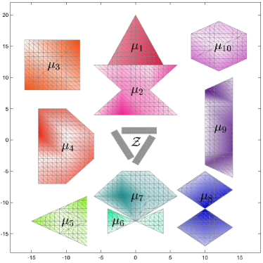
Figure 4.1. Experiment 1 – Probability density functions of the probability measures $\mu_{1}\in\mathcal{P}(\mathcal{X}_{1}),\ldots,$ $\mu_{N}\in\mathcal{P}(\mathcal{X}_{N})$ and the triangulations used for defining the test functions $\mathcal{G}_{1},\ldots,\mathcal{G}_{N},\mathcal{H}$.

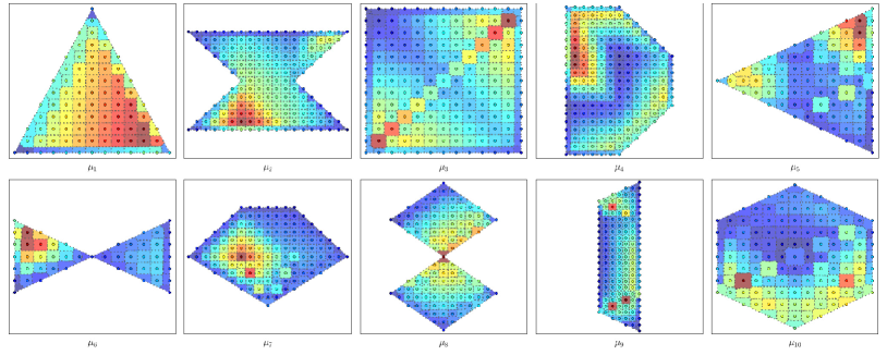
Figure 4.2. Experiment 1 – Laguerre diagrams characterizing the computed optimal couplings between the probability measures $\hat{\mu}_{i}\in\mathcal{P}(\mathcal{X}_{i})$ and $\mu_{i}\in\mathcal{P}(\mathcal{X}_{i})$ for $i=1,\ldots,N$. The color of each cell shows the probability mass contained in the cell, where blue indicates low probability and red indicates high probability.

Due to the structure of the cost functions $c_{1},\ldots,c_{N}$, we can derive the following proposition.

Proposition 4.2.

Let Assumption 4.1 hold. Then, for $i=1,\ldots,N$ and for any ${\bm{y}}_{i}\in\mathbb{R}^{m_{i}}$, ${\bm{w}}_{i}\in\mathbb{R}^{k}$, it holds that

$$\inf_{{\bm{x}}_{i}\in\mathcal{X}_{i},\,{\bm{z}}_{i}\in\mathcal{Z}}\big{\{}c_{i}({\bm{x}}_{i},{\bm{z}}_{i})-\langle{\bm{g}}_{i}({\bm{x}}_{i}),{\bm{y}}_{i}\rangle-\langle{\bm{h}}({\bm{z}}_{i}),{\bm{w}}_{i}\rangle\big{\}}$$

$$\qquad\qquad=\min_{{\bm{x}}_{i}\in V(\mathfrak{C}_{i}),\,{\bm{z}}_{i}\in\mathcal{Z}}\big{\{}c_{i}({\bm{x}}_{i},{\bm{z}}_{i})-\langle{\bm{g}}_{i}({\bm{x}}_{i}),{\bm{y}}_{i}\rangle-\langle{\bm{h}}({\bm{z}}_{i}),{\bm{w}}_{i}\rangle\big{\}}.$$

Proof of Proposition 4.2.

See Appendix A.2. ∎

In Algorithm 1, it follows from Proposition 4.2 that we may restrict the set $\mathcal{C}_{i}^{\star(r)}$ in Line 1 to be a subset of $V(\mathfrak{C}_{i})\times\mathcal{Z}$ while preserving its correctness. Subsequently, for $i=1\ldots,N$, the output $\hat{\theta}_{i}$ of Algorithm 1 will be a discrete probability measure with support in $V(\mathfrak{C}_{i})\times\mathcal{Z}$. Since the marginal of $\hat{\theta}_{i}$ on $\mathcal{X}_{i}$ is required to be in $[\mu_{i}]_{\mathcal{G}_{i}}$ by Proposition 3.5(v), one can check that the marginal of $\hat{\theta}_{i}$ on $\mathcal{X}_{i}$ must be equal to $\hat{\mu}_{i}$, given by:

$$\hat{\mu}_{i}=\sum_{j=0}^{m_{i}}\bigg{(}\int_{\mathcal{X}_{i}}g_{i,{\bm{v}}_{i,j}}\,\mathrm{d}{\mu_{i}}\bigg{)}\delta_{{\bm{v}}_{i,j}},$$

which only depends on $\mu_{i}$ and $\mathcal{G}_{i}$. In Line 2 of Algorithm 2, an optimal coupling of $\hat{\mu}_{i}$ and $\mu_{i}$ is constructed via Lemma 3.1. Since $\hat{\mu}_{i}$ is discrete and $\mu_{i}$ is continuous, this corresponds to the discrete-to-continuous case (C2) in Lemma 3.1. Thus, an optimal coupling of $\hat{\mu}_{i}$ and $\mu_{i}$ can be characterized by (3.3) via subsets of $\mathcal{X}_{i}$ defined in (3.2), which are referred to as cells in a Laguerre diagram. Figure 4.2 shows the Laguerre diagrams characterizing the computed optimal couplings of $\hat{\mu}_{i}$ and $\mu_{i}$ for $i=1,\ldots,N$, where the partitions $\mathfrak{C}_{1},\ldots,\mathfrak{C}_{N}$ of $\mathcal{X}_{1},\ldots,\mathcal{X}_{N}$ are identical to those shown in Figure 4.1. In Figure 4.2, each circle represents an atom in the discrete measure $\hat{\mu}_{i}$, where the color of the circle represents the probability of that atom. The cell surrounding each atom corresponds to the cell in the computed Laguerre diagram that the atom is coupled with. These Laguerre diagrams allow independent random samples to be efficiently generated from the couplings $(\hat{\gamma}_{i})_{i=1:N}$ and $(\tilde{\gamma}_{i})_{i=1:N}$ via (3.3) in Lemma 3.1 and rejection sampling. This subsequently allows $\hat{\alpha}_{\mathsf{MT}}^{\mathsf{U}\mathsf{B}}$ and $\tilde{\alpha}_{\mathsf{MT}}^{\mathsf{U}\mathsf{B}}$ in Line 2 of Algorithm 2 to be efficiently and accurately approximated via Monte Carlo integration.

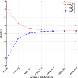
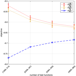
Figure 4.3. Experiment 1 – Left: the computed upper and lower bounds for the optimal value of ($\mathsf{M}\mathsf{T}$). Center: magnification of the rightmost part of the left panel. Right: the computed sub-optimality estimates of Algorithm 2.

In order to compute approximate matching equilibria for this matching for teams problem, we fix $\epsilon=0.005$ and test 7 different combinations of test functions resulted from partitions $\mathfrak{C}_{0},\mathfrak{C}_{1},\ldots,\mathfrak{C}_{N}$ of the sets $\mathcal{Z},\mathcal{X}_{1},\ldots,\mathcal{X}_{N}$. Specifically, the test functions in $\mathcal{G}_{1},\ldots,\mathcal{G}_{N}$ are defined based on increasingly finer partitions of $\mathcal{X}_{1},\ldots,\mathcal{X}_{N}$, and the value of $|\mathcal{G}_{1}|+\cdots+|\mathcal{G}_{N}|$ ranges between 60 and 4800. Moreover, the test functions in $\mathcal{H}$ are defined based on increasingly finer partitions of $\mathcal{Z}$, and the value of $|\mathcal{H}|$ ranges between 35 and 863. The values of $\hat{\alpha}_{\mathsf{MT}}^{\mathsf{U}\mathsf{B}}$, $\tilde{\alpha}_{\mathsf{MT}}^{\mathsf{U}\mathsf{B}}$ in Line 2 of Algorithm 2 are computed via Monte Carlo integration using $10^{6}$ independent random samples. Moreover, each Monte Carlo integration is repeated 100 times in order to examine the Monte Carlo error.

Figure 4.3 shows the computed upper and lower bounds for ($\mathsf{M}\mathsf{T}$), the sub-optimality estimates $\hat{\epsilon}_{\mathsf{MT}}$, $\tilde{\epsilon}_{\mathsf{MT}}$, and their a priori theoretical upper bound $\epsilon^{\ddagger}_{\overline{\overline{W}}_{1}}$ given by

$$\epsilon^{\ddagger}_{\overline{\overline{W}}_{1}} :=\epsilon+\frac{4}{N}\max_{{\bm{z}}\in\mathcal{Z}}\big{\{}\|{\bm{z}}\|_{2}\big{\}}\Bigg{(}\sum_{i=1}^{N}\max_{C\in\mathfrak{C}_{i}}\max_{{\bm{x}},{\bm{x}}^{\prime}\in C}\big{\{}\|{\bm{x}}-{\bm{x}}^{\prime}\|_{2}\big{\}}\Bigg{)}$$

$$\qquad\qquad+\Bigg{[}\frac{4(N-1)}{N}\max_{{\bm{z}}\in\mathcal{Z}}\big{\{}\|{\bm{z}}\|_{2}\big{\}}+\frac{4}{N}\sum_{i\neq\hat{i}}\max_{{\bm{x}}_{i}\in\mathcal{X}_{i}}\big{\{}\|{\bm{x}}_{i}\|_{2}\big{\}}\Bigg{]}\max_{C\in\mathfrak{C}_{0}}\max_{{\bm{z}},{\bm{z}}^{\prime}\in C}\big{\{}\|{\bm{z}}-{\bm{z}}^{\prime}\|_{2}\big{\}}.$$

Note that the a priori theoretical upper bound $\epsilon^{\ddagger}_{\overline{\overline{W}}_{1}}$ is derived from Theorem 3.7(vi) with

$$L_{c_{i}}^{(1)} :=\frac{2}{N}\max_{{\bm{z}}\in\mathcal{Z}}\big{\{}\|{\bm{z}}\|_{2}\big{\}}\hskip 124.0pt\qquad\forall 1\leq i\leq N,$$

$$L_{c_{i}}^{(2)} :=\frac{2}{N}\Big{(}\max_{{\bm{z}}\in\mathcal{Z}}\big{\{}\|{\bm{z}}\|_{2}\big{\}}+\max_{{\bm{x}}\in\mathcal{X}_{i}}\big{\{}\|{\bm{x}}\|_{2}\big{\}}\Big{)}\hskip 39.5pt\qquad\forall 1\leq i\leq N,$$

$$\overline{\overline{W}}_{1,\mu_{i}} :=2\max_{C\in\mathfrak{C}_{i}}\max_{{\bm{x}},{\bm{x}}^{\prime}\in C}\big{\{}\|{\bm{x}}-{\bm{x}}^{\prime}\|_{2}\big{\}}\geq\overline{W}_{1,\mu_{i}}\big{(}[\mu_{i}]_{\mathcal{G}_{i}}\big{)}\qquad\forall 1\leq i\leq N,$$

$$\overline{\overline{W}}_{1,\mathcal{Z}} :=2\max_{C\in\mathfrak{C}_{0}}\max_{{\bm{z}},{\bm{z}}^{\prime}\in C}\big{\{}\|{\bm{z}}-{\bm{z}}^{\prime}\|_{2}\big{\}}\geq\sup\Big{\{}W_{1}(\nu,\nu^{\prime}):\nu,\nu^{\prime}\in\mathcal{P}(\mathcal{Z}),\;\nu\overset{\mathcal{H}}{\sim}\nu^{\prime}\Big{\}}.$$

The left panel of Figure 4.3 shows the upper bounds $\hat{\alpha}_{\mathsf{MT}}^{\mathsf{U}\mathsf{B}}$, $\tilde{\alpha}_{\mathsf{MT}}^{\mathsf{U}\mathsf{B}}$ and the lower bound $\alpha_{\mathsf{MT}}^{\mathsf{L}\mathsf{B}}$ computed by Algorithm 2. The horizontal axis shows the number of test functions used, i.e., each tuple corresponds to ${\big{(}|\mathcal{G}_{1}|+\cdots+|\mathcal{G}_{N}|,|\mathcal{H}|\big{)}}$. It can be seen that the differences between the upper bounds and the lower bound are initially large when $|\mathcal{G}_{1}|+\cdots+|\mathcal{G}_{N}|=60$ and $|\mathcal{H}|=35$. When $|\mathcal{G}_{1}|+\cdots+|\mathcal{G}_{N}|$ and $|\mathcal{H}|$ both increase, the difference between the bounds decreases. When $|\mathcal{G}_{1}|+\cdots+|\mathcal{G}_{N}|=4800$ and $|\mathcal{H}|=863$, the values of the computed sub-optimality estimates $\hat{\epsilon}_{\mathsf{MT}}$ and $\tilde{\epsilon}_{\mathsf{MT}}$ are $0.0633$ and $0.0582$, respectively. By Theorem 2.15, this shows that $\big{(}(\tilde{\varphi}_{i})_{i=1:N}$, $(\hat{\gamma}_{i})_{i=1:N}$, $\hat{\nu}\big{)}$ and $\big{(}(\tilde{\varphi}_{i})_{i=1:N}$, $(\tilde{\gamma}_{i})_{i=1:N}$, $\tilde{\nu}\big{)}$ computed by Algorithm 2 are approximate matching equilibria that are close to true matching equilibria. The center panel of Figure 4.3 shows a magnification of the left panel, with error bars indicating the 95% intervals of Monte Carlo integration. From the results, it can be observed that the differences between the two upper bounds $\hat{\alpha}_{\mathsf{MT}}^{\mathsf{U}\mathsf{B}}$ and $\tilde{\alpha}_{\mathsf{MT}}^{\mathsf{U}\mathsf{B}}$ are small. The right panel of Figure 4.3 compares the computed sub-optimality estimates $\hat{\epsilon}_{\mathsf{MT}}$ and $\tilde{\epsilon}_{\mathsf{MT}}$ with their a priori theoretical upper bound $\epsilon^{\ddagger}_{\overline{\overline{W}}_{1}}$ on the log-scale. The results show that the value of $\epsilon^{\ddagger}_{\overline{\overline{W}}_{1}}$ is one to two orders of magnitude larger than $\hat{\epsilon}_{\mathsf{MT}}$ and $\tilde{\epsilon}_{\mathsf{MT}}$. This demonstrates that not only does Algorithm 2 produce feasible solutions of ($\mathsf{M}\mathsf{T}$), ($\mathsf{M}\mathsf{T}^{*}$), and ($\mathsf{M}\mathsf{T}_{\mathsf{cp}}$), it also produces sub-optimality estimates $\hat{\epsilon}_{\mathsf{MT}}$, $\tilde{\epsilon}_{\mathsf{MT}}$ of these feasible solutions that are much less conservative than suggested by an a priori theoretical analysis, as discussed in Remark 3.8. Specifically, when $|\mathcal{G}_{1}|+\cdots+|\mathcal{G}_{N}|=4800$ and $|\mathcal{H}|=863$, the value of $\epsilon^{\ddagger}_{\overline{\overline{W}}_{1}}$ is equal to $28.8769$, which indicates that the solutions computed by Algorithm 2 could be poor. Despite that, the sub-optimality estimates $\hat{\epsilon}_{\mathsf{MT}}$ and $\tilde{\epsilon}_{\mathsf{MT}}$ computed by Algorithm 2 are equal to $0.0633$ and $0.0582$, respectively, indicating that $\big{(}(\tilde{\varphi}_{i})_{i=1:N},(\hat{\gamma}_{i})_{i=1:N},\hat{\nu}\big{)}$ and $\big{(}(\tilde{\varphi}_{i})_{i=1:N},(\tilde{\gamma}_{i})_{i=1:N},\tilde{\nu}\big{)}$ are close to being optimal.

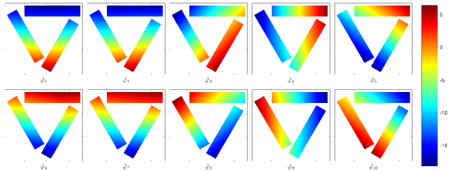
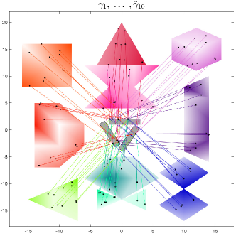
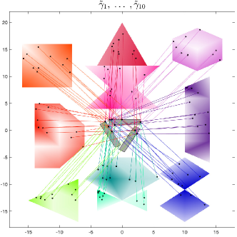
Figure 4.4. Experiment 1 – Top: heat maps showing the approximately optimal transfer functions $(\tilde{\varphi}_{i})_{i=1:N}$. Bottom: random samples from the approximately optimal couplings $(\hat{\gamma}_{i})_{i=1:N}$, $(\tilde{\gamma}_{i})_{i=1:N}$ computed by Algorithm 2. The solid lines in the bottom panel indicate the coupling between sample points in $\mathcal{X}_{1},\ldots,\mathcal{X}_{N},\mathcal{Z}$.

Finally, Figure 4.4 shows the approximately optimal transfer functions $(\tilde{\varphi}_{i})_{i=1:N}$ and the approximately optimal couplings $(\hat{\gamma}_{i})_{i=1:N}$, $(\tilde{\gamma}_{i})_{i=1:N}$ computed by Algorithm 2 when $|\mathcal{G}_{1}|+\cdots+|\mathcal{G}_{N}|=4800$ and $|\mathcal{H}|=863$. The top panel of Figure 4.4 shows the values of the functions $(\tilde{\varphi}_{i})_{i=1:N}$ in color plots. The bottom-left panel shows independent realizations from the random variable $(\bar{X}_{1},\ldots,\bar{X}_{N},Z)$ constructed by Algorithm 2. They can be seen as coupled random samples from the probability measures $(\hat{\gamma}_{i})_{i=1:N}$. The bottom-right panel shows independent realizations from the random variable $(\bar{X}_{1},\ldots,\bar{X}_{N},\bar{Z})$ constructed by Algorithm 2. They can be seen as coupled random samples from the probability measures $(\tilde{\gamma}_{i})_{i=1:N}$. These samples also demonstrate how agents from the 10 categories are matched together to form teams.

When we adopt the interpretation of the matching for teams problem as an economic game of locating business outlets described in Example 1.3, up to additions of constants that sum up to 0, the functions $\tilde{\varphi}_{1},\ldots,\tilde{\varphi}_{N-1}$ represent the amount of salary earned by the employees from the categories $1,\ldots,N-1$ working at each location of business outlet, and the function $\tilde{\varphi}_{N}$ represents the negative of the total amount of salary paid out at each location of business outlet. Since for $i=1,\ldots,N-1$, the commuting cost $c_{i}({\bm{x}}_{i},{\bm{z}}):=\frac{1}{N}\big{(}\|{\bm{z}}\|_{2}^{2}-2\langle{\bm{x}}_{i},{\bm{z}}\rangle\big{)}=\frac{1}{N}\|{\bm{x}}_{i}-{\bm{z}}\|_{2}^{2}-\frac{1}{N}\|{\bm{x}}_{i}\|_{2}^{2}$ is equal to the scaled squared Euclidean distance $\frac{1}{N}\|{\bm{x}}_{i}-{\bm{z}}\|_{2}^{2}$ minus a term $\frac{1}{N}\|{\bm{x}}_{i}\|_{2}^{2}$ that does not affect the matching, employees working at business outlets that are further from home will be paid more salary compared to employees working at business outlets closer to home. This can be observed from Figure 4.4. For example, since $\mathcal{X}_{1}$ is located to the north of $\mathcal{Z}$ (see Figure 4.1), for an employee from category 1, the south part of $\mathcal{Z}$ is further away compared to the north part of $\mathcal{Z}$. Therefore, it can be observed from Figure 4.4 that the value of $\tilde{\varphi}_{1}$ is larger in the south part of $\mathcal{Z}$ compared to the north part of $\mathcal{Z}$. Similarly, since the restocking cost $c_{N}({\bm{x}}_{N},{\bm{z}}):=\frac{1}{N}\big{(}\|{\bm{z}}\|_{2}^{2}-2\langle{\bm{x}}_{N},{\bm{z}}\rangle\big{)}=\frac{1}{N}\|{\bm{x}}_{N}-{\bm{z}}\|_{2}^{2}-\frac{1}{N}\|{\bm{x}}_{N}\|_{2}^{2}$ is also equal to the scaled squared Euclidean distance $\frac{1}{N}\|{\bm{x}}_{N}-{\bm{z}}\|_{2}^{2}$ minus a term $\frac{1}{N}\|{\bm{x}}_{N}\|_{2}^{2}$ that does not affect the matching, business outlets that are closer to the suppliers will pay more salary to their employees compared to business outlets that are further from the suppliers at an approximate matching equilibrium. This can also be observed from the relative positions of $\mathcal{X}_{10}$ and $\mathcal{Z}$ in Figure 4.1 and the values of $\tilde{\varphi}_{10}$ in Figure 4.4. These experimental results can not only provide insights for the business owners to decide where to locate the business outlets, but also aid city planners in building future public transportation systems in the city.

4.2. Experiment 2

In the second numerical experiment, we examine the scalability of Algorithm 1 in terms of how its running time changes with the number $N$ of agent categories in the matching for teams problem. Specifically, we consider the following setting.

Assumption 4.3 (Numerical experiment with one-dimensional type spaces).

We assume that the following statements hold.

• For $i=1,\ldots,N$, $\mathcal{X}_{i}=[\underline{\kappa}_{i},\overline{\kappa}_{i}]\subset\mathbb{R}$, where $-\infty<\underline{\kappa}_{i}<\overline{\kappa}_{i}<\infty$. Moreover, $d_{\mathcal{X}_{i}}(x_{i},x^{\prime}_{i}):=|x_{i}-x^{\prime}_{i}|$.

• $\mathcal{Z}=\bigcup_{C\in\mathfrak{C}_{0}}C\subset\mathbb{R}^{2}$ is a polytope, where $\mathfrak{C}_{0}$ is a finite collection of triangles such that whenever $C_{1}\cap C_{2}\neq\emptyset$ for distinct $C_{1},C_{2}\in\mathfrak{C}_{0}$ then $C_{1}\cap C_{2}$ is a face (i.e., a vertex or an edge) of $C_{1}$ and $C_{2}$. Moreover, $d_{\mathcal{Z}}({\bm{z}},{\bm{z}}^{\prime}):=\|{\bm{z}}-{\bm{z}}^{\prime}\|_{2}$.

• For $i=1,\ldots,N$, $\mu_{i}\in\mathcal{P}(\mathcal{X}_{i})$ is absolutely continuous with respect to the Lebsegue measure on $\mathcal{X}_{i}$ and $\mathrm{supp}(\mu_{i})=\mathcal{X}_{i}$.

• For $i=1,\ldots,N$, $c_{i}:\mathcal{X}_{i}\times\mathcal{Z}\to\mathbb{R}$ is given by $c_{i}(x_{i},{\bm{z}}):=l_{i}\big{(}x_{i}-\langle{\bm{s}}_{i},{\bm{z}}\rangle\big{)}$ where ${\bm{s}}_{i}\in\mathbb{R}^{2}$ and $l_{i}:[\lambda_{i,0},\lambda_{i,n_{i}}]\to\mathbb{R}$ is a continuous function that is piece-wise affine on $[\lambda_{i,0},\lambda_{i,1}],\ldots,[\lambda_{i,n_{i}-1},\lambda_{i,n_{i}}]$ for $n_{i}\in\mathbb{N}$, $-\infty<\lambda_{i,0}<\lambda_{i,1}<\cdots<\lambda_{i,n_{i}}<\infty$, satisfying $\lambda_{i,0}\leq\underline{\kappa}_{i}-\max_{{\bm{z}}\in\mathcal{Z}}\big{\{}\langle{\bm{s}}_{i},{\bm{z}}\rangle\big{\}}$, $\lambda_{i,n_{i}}\geq\overline{\kappa}_{i}-\min_{{\bm{z}}\in\mathcal{Z}}\big{\{}\langle{\bm{s}}_{i},{\bm{z}}\rangle\big{\}}$.

• For $i=1,\ldots,N$, $\underline{\kappa}_{i}=\kappa_{i,0}<\kappa_{i,1}<\cdots<\kappa_{i,m_{i}}=\overline{\kappa}_{i}$, and $g_{i,0},g_{i,1},\ldots,g_{i,m_{i}}:\mathcal{X}_{i}\to\mathbb{R}$ are defined as follows:

  $$g_{i,0}(x_{i}) :=\frac{(\kappa_{i,1}-x_{i})^{+}}{\kappa_{i,1}-\kappa_{i,0}},$$

  $$g_{i,j}(x_{i}) :=\min\left\{\frac{(x_{i}-\kappa_{i,j-1})^{+}}{\kappa_{i,j}-\kappa_{i,j-1}},\frac{(\kappa_{i,j+1}-x_{i})^{+}}{\kappa_{i,j+1}-\kappa_{i,j}}\right\}\qquad\forall 1\leq j\leq m_{i}-1,$$

  $$g_{i,m_{i}}(x_{i}) :=\frac{(x_{i}-\kappa_{i,m_{i}-1})^{+}}{\kappa_{i,m_{i}}-\kappa_{i,m_{i}-1}}.$$

  Let $\mathcal{G}_{i}:=\{g_{i,1},\ldots,g_{i,m_{i}}\}$ and let ${\bm{g}}_{i}(x_{i}):=\big{(}g_{i,1}(x_{i}),\ldots,g_{i,m_{i}}(x_{i})\big{)}^{\mathsf{T}}$ for all $x_{i}\in\mathcal{X}_{i}$.

• Let $\{{\bm{v}}_{0,0},{\bm{v}}_{0,1},\ldots,{\bm{v}}_{0,k}\}$ be an arbitrary enumeration of the finite set $V(\mathfrak{C}_{0}):=\big{\{}{\bm{v}}\in\mathbb{R}^{2}:{\bm{v}}$ is an extreme point of some $C\in\mathfrak{C}_{0}\big{\}}$ (i.e., the cardinality of this set is $k+1\in\mathbb{N}$), let $\mathcal{H}:=\big{\{}h_{{\bm{v}}_{0,1}},\ldots,h_{{\bm{v}}_{0,k}}\big{\}}$, and let ${\bm{h}}({\bm{z}}):=\big{(}h_{{\bm{v}}_{0,1}}({\bm{z}}),\ldots,h_{{\bm{v}}_{0,k}}({\bm{z}})\big{)}^{\mathsf{T}}$ for all ${\bm{z}}\in\mathcal{Z}$, where the functions $(h_{{\bm{v}}_{0,l}}:\mathcal{Z}\to\mathbb{R})_{l=1:k}$ are defined in Theorem 2.17(vii).

In particular, these statements imply that Assumption 3.2 is satisfied.

Thus, under Assumption 4.3, the spaces $\mathcal{X}_{1},\ldots,\mathcal{X}_{N}$ representing agent types are all one-dimensional, while the quality space $\mathcal{Z}$ is two-dimensional. In order to investigate the performance of our method, we independently randomly generate 10 problem instances (or scenarios) as follows:

• each $\mu_{i}$ is a probability measure on the closed interval $[0,1]$ with a probability density function that is continuous and piece-wise affine on the intervals $\big{[}0,\frac{1}{4}\big{]}$, $\big{[}\frac{1}{4},\frac{1}{2}\big{]}$, $\big{[}\frac{1}{2},\frac{3}{4}\big{]}$, $\big{[}\frac{3}{4},1\big{]}$, where the values of the density function at the points $0,\frac{1}{4},\frac{1}{2},\frac{3}{4},1$ are randomly generated;

• $\mathcal{Z}=\mathrm{conv}\Big{(}\Big{\{}\big{(}\begin{smallmatrix}0\\ 0\end{smallmatrix}\big{)},\big{(}\begin{smallmatrix}1\\ 0\end{smallmatrix}\big{)},\big{(}\begin{smallmatrix}0\\ 1\end{smallmatrix}\big{)}\Big{\}}\Big{)}$;

• each ${\bm{s}}_{i}\in\mathbb{R}^{2}$ is a random point on the unit circle and each $l_{i}(\cdot)$ is defined by

  $$l_{i}(t):=\begin{cases}0&\text{if }|t|\leq\theta_{i,1},\\ \frac{1}{N}\big{(}|t|-\theta_{i,1}\big{)}&\text{if }\theta_{i,1}<|t|\leq\theta_{i,2},\\ \frac{1}{N}(\theta_{i,2}-\theta_{i,1})&\text{if }|t|>\theta_{i,2},\end{cases}$$

  where $\theta_{i,2}>\theta_{i,1}>0$ are randomly generated constants;

• for each $i$, $m_{i}=49$ and $\kappa_{i,0}<\kappa_{i,1}<\cdots<\kappa_{i,m_{i}}$ are 50 evenly-spaced points in $[0,1]$;

• $k=560$ and $\{{\bm{v}}_{0,0},{\bm{v}}_{0,1},\ldots,{\bm{v}}_{0,k}\}$ form an evenly-spaced two-dimensional grid of 561 points in $\mathcal{Z}$.

The choice of the function $l_{i}$ reflects a practical interpretation of the matching for teams problem under Assumption 4.3. In this problem, each unit of good is characterized by its two qualities in $\mathcal{Z}$. For each $i$, each agent within the $i$-th category has a randomly distributed latent preference variable $x_{i}\in\mathcal{X}_{i}$, and the vector ${\bm{s}}_{i}\in\mathbb{R}^{2}$ represents the weights these agents use to assess the qualities of goods. The cost function $c_{i}(x_{i},{\bm{z}})$ depends on the absolute difference between the agent’s preference $x_{i}$ and the agent’s assessment $\langle{\bm{s}}_{i},{\bm{z}}\rangle$, where the cost is 0 if $\big{|}x_{i}-\langle{\bm{s}}_{i},{\bm{z}}\rangle\big{|}$ is below a threshold $\theta_{i,1}$, the cost grows linearly when $\big{|}x_{i}-\langle{\bm{s}}_{i},{\bm{z}}\rangle\big{|}$ is above the threshold $\theta_{i,1}$ but below a second threshold $\theta_{i,2}$, and the cost remains constant when $\big{|}x_{i}-\langle{\bm{s}}_{i},{\bm{z}}\rangle\big{|}$ exceeds the second threshold $\theta_{i,2}$.

In this experiment, we fix $\epsilon=5\times 10^{-5}$. It follows from the definition that $c_{i}$ is $\frac{1}{N}$-Lipschitz continuous (with respect to the 1-product metric on $\mathcal{X}_{i}\times\mathcal{Z}$). Therefore, we define the a priori theoretical upper bound $\epsilon^{\ddagger}_{\overline{\overline{W}}_{1}}$ by

$$\epsilon^{\ddagger}_{\overline{\overline{W}}_{1}} :=\epsilon+\left(\sum_{i=1}^{N}\frac{2}{N}\max_{1\leq j\leq m_{i}}\{\kappa_{i,j}-\kappa_{i,j-1}\}\right)+\left(\sum_{i=1}^{N}\frac{1}{N}\right)2\max_{C\in\mathfrak{C}_{0}}\max_{{\bm{z}},{\bm{z}}^{\prime}\in C}\big{\{}\|{\bm{z}}-{\bm{z}}^{\prime}\|_{2}\big{\}}$$

$$\phantom{:}=\epsilon+\frac{2}{m_{1}}+2\max_{C\in\mathfrak{C}_{0}}\max_{{\bm{z}},{\bm{z}}^{\prime}\in C}\big{\{}\|{\bm{z}}-{\bm{z}}^{\prime}\|_{2}\big{\}}$$

$$\phantom{:}=0.1293,$$

which remains constant for all values of $N$.

In Algorithm 1 The global minimization problem $\mathtt{Oracle}(\cdot,\,\cdot,\,\cdot)$ in Definition 2.1 is formulated into a mixed-integer programming problem and are subsequently solved by the mixed-integer solver of Gurobi [43]. We would like to remark that the global minimization problems $\mathtt{Oracle}\big{(}1,{\bm{y}}_{1}^{(r)},{\bm{w}}_{1}^{(r)}\big{)},\ldots,\mathtt{Oracle}\big{(}N,{\bm{y}}_{N}^{(r)},{\bm{w}}_{N}^{(r)}\big{)}$ in Line 1 of Algorithm 1 can be solved in parallel. However, we choose to solve them sequentially in our implementation of Algorithm 1 in order not to over-complicate the running time analysis.

We apply Algorithm 2 to the 10 randomly generated problem instances and record the computed values of the sub-optimality estimate $\hat{\epsilon}_{\mathsf{MT}}$ as well as the running time of Algorithm 1 for $N=4,6,8,10,12,14,16,18,20,50,80,100$ agent categories. $\hat{\epsilon}_{\mathsf{MT}}$ is computed via Monte Carlo integration using $10^{7}$ independent samples. We only examine the values of $\hat{\epsilon}_{\mathsf{MT}}$ here because $\tilde{\epsilon}_{\mathsf{MT}}\leq\hat{\epsilon}_{\mathsf{MT}}$ and the computation of $\tilde{\epsilon}_{\mathsf{MT}}$ requires us to solve a global minimization problem (2.5), which is more computationally costly than the computation of $\hat{\epsilon}_{\mathsf{MT}}$. In addition, we only examine the running time of Line 2 in Algorithm 2, i.e., the running time of Algorithm 1. The running time of the rest of Algorithm 2 consists mostly of time spent computing $\hat{\alpha}_{\mathsf{MT}}^{\mathsf{U}\mathsf{B}}$ via Monte Carlo integration in Line 2, which can be parallelized and is negligible compared to the running time of Line 2 when $N$ is large.

Table 4.1. Experiment 2 – Computed sub-optimality estimate, running time of Algorithm 1, and support sparsity (note that $\epsilon^{\ddagger}_{\overline{\overline{W}}_{1}}=0.1293$).

	Avg. $\hat{\epsilon}_{\mathsf{MT}}$	Max. $\hat{\epsilon}_{\mathsf{MT}}$	Avg.	Max.	Avg.	Max.	$\min_{1\leq i\leq N}\{m_{i}\}$
$N$	[$\times 10^{-4}$]	[$\times 10^{-4}$]	time [s]	time [s]	$|\mathrm{supp}(\hat{\nu})|$	$|\mathrm{supp}(\hat{\nu})|$	$+k+2$
4	9.771	26.625	537	1123	87.1	104	611
6	10.636	23.440	1283	2438	104.8	137	611
8	7.319	11.492	1958	2781	99.9	132	611
10	8.419	16.667	2820	3542	113.0	161	611
12	8.557	20.180	3834	4377	114.8	168	611
14	8.291	17.612	4695	5513	118.3	176	611
16	7.461	15.005	5826	7629	116.1	170	611
18	6.999	12.227	6462	7398	109.3	164	611
20	6.869	12.815	6884	8009	120.6	203	611
50	5.464	6.968	17462	19717	140.1	175	611
80	4.927	6.355	33949	38496	151.1	187	611
100	4.822	6.412	42348	49769	156.8	205	611

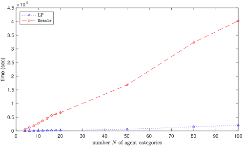
Figure 4.5. Experiment 2 – Running time of the LP solver (Line 1) and the global minimization oracle (Line 1) in Algorithm 1.

The left part of Table 4.1 shows the average and maximum sub-optimality estimates and the average and maximum running time of Algorithm 1 when $N=4,6,8,10,12,14,16,18,20,50,80,100$. From the results, it can be seen that the values of the sub-optimality estimate $\hat{\epsilon}_{\mathsf{MT}}$ computed by our algorithm are about two orders of magnitude smaller than the a priori theoretical upper bound $\epsilon^{\ddagger}_{\overline{\overline{W}}_{1}}=0.1293$.

Figure 4.5 shows the total running time of the LP solver in Line 1 of Algorithm 1, and the total running time of $\mathtt{Oracle}(\cdot,\,\cdot,\,\cdot)$ in Line 1 of Algorithm 1. It can be seen that the total running time of $\mathtt{Oracle}(\cdot,\,\cdot,\,\cdot)$ in Algorithm 1 is much longer relative to the LP solver for all values of $N$, showing that almost all of the running time is spent on computing $\mathtt{Oracle}(\cdot,\,\cdot,\,\cdot)$. An interesting observation is that the total running time of $\mathtt{Oracle}(\cdot,\,\cdot,\,\cdot)$ seems to grow approximately linearly in $N$. This is in line with our discussion in Remark 2.4. Under Assumption 4.3, for $i=1,\ldots,N$ and for ${\bm{y}}_{i}\in\mathbb{R}^{m_{i}}$, ${\bm{w}}_{i}\in\mathbb{R}^{k}$, the global minimization problem $\mathtt{Oracle}(\cdot,\,\cdot,\,\cdot)$ is given by

$$\operatorname*{\mathrm{minimize}}_{x_{i},\,{\bm{z}}_{i}}\quad l_{i}\big{(}x_{i}-\langle{\bm{s}}_{i},{\bm{z}}_{i}\rangle\big{)}-\langle{\bm{g}}_{i}(x_{i}),{\bm{y}}_{i}\rangle-\langle{\bm{h}}({\bm{z}}_{i}),{\bm{w}}_{i})\rangle$$

subject to $$\underline{\kappa}_{i}\leq x_{i}\leq\overline{\kappa}_{i},$$

$${\bm{z}}_{i}\in\mathcal{Z},$$

which corresponds to minimizing a continuous piece-wise affine function with 3 variables, since $\mathcal{X}_{i}\times\mathcal{Z}\subset\mathbb{R}^{3}$. Thus, the computational cost of this minimization indeed does not depend on $N$. Since each iteration of Algorithm 1 solves $N$ such minimization problems, the total running time of $\mathtt{Oracle}(\cdot,\,\cdot,\,\cdot)$ in each iteration of Algorithm 1 increases linearly in $N$. In addition, in Algorithm 1, the number of iterations till convergence grows slowly relative to the growth of $N$, which makes the total running time of $\mathtt{Oracle}(\cdot,\,\cdot,\,\cdot)$ in Algorithm 1 grow approximately linearly in $N$. Moreover, this shows that in a computing environment with sufficient parallelization capabilities, a suitable parallel implementation of the for-loop in Line 1 can drastically reduce the running time of Algorithm 1.

Remark 4.4.

The LP problem ($\mathsf{M}\mathsf{T}^{*(r)}_{\mathsf{par}}$) that is solved in Line 1 of Algorithm 1 has a structure which allows it to be efficiently solved by parallel algorithms based on operator splitting methods; see, e.g., [33]. In this experiment, we use the standard LP solver provided by Gurobi [43] since it is reasonably efficient. The investigation of the parallelization aspects of Algorithm 1 is left as future work.

Furthermore, recall that we have shown in Corollary 2.13 the existence of an approximate optimizer $\hat{\nu}$ of ($\mathsf{M}\mathsf{T}$) with $|\mathrm{supp}(\hat{\nu})|\leq\min_{1\leq i\leq N}\{m_{i}\}+k+2$. The right part of Table 4.1 shows the average and maximum values of $|\mathrm{supp}(\hat{\nu})|$, where $\hat{\nu}$ is the discrete approximate optimizer of ($\mathsf{M}\mathsf{T}$) computed by Algorithm 2. It shows that $\hat{\nu}$ computed by Algorithm 2 is even more sparse than what Corollary 2.13 suggests, even though $|\mathrm{supp}(\hat{\nu})|$ still increases with $N$. A possible explanation of the latter phenomenon is as follows. As discussed by Carlier et al. [24, Section 2.2], one can restrict the quality space $\mathcal{Z}$ to any subset $\mathcal{Z}^{\prime}\subseteq\mathcal{Z}$ satisfying $\mathcal{Z}^{\prime}\supseteq\tilde{z}({\bm{\mathcal{X}}})$ without affecting the optimal value of ($\mathsf{M}\mathsf{T}$). This suggests that there could be many test functions in $\mathcal{H}$ that are redundant since they are identical when their domains are restricted to a suitable choice of $\mathcal{Z}^{\prime}$.

Appendix A Proof of theoretical results

A.1. Proof of results in Section 2

Proof of Theorem 2.

This proof is based on the theoretical computational complexity of the cutting-plane algorithm of Vaidya [66]. In order to apply the theory of Vaidya [66], we will need the superlevel sets of ($\mathsf{M}\mathsf{T}^{*}_{\mathsf{par}}$) to contain a Euclidean ball, which is prevented by the presence of the equality constraint $\sum_{i=1}^{N}{\bm{w}}_{i}=\mathbf{0}_{k}$. Therefore, we will first show that, under the assumption that the functions $h_{1},\ldots,h_{k}$ are all non-negative, we can relax the equality constraint into an inequality constraint $\sum_{i=1}^{N}{\bm{w}}_{i}\geq\mathbf{0}_{k}$, that is, we will show that the optimal value of ($\mathsf{M}\mathsf{T}^{*}_{\mathsf{par}}$) is equal to the optimal value of the following problem:

$$\begin{split}\operatorname*{\mathrm{maximize}}_{(y_{i,0},{\bm{y}}_{i},{\bm{w}}_{i})}\quad&\sum_{i=1}^{N}y_{i,0}+\langle\bar{{\bm{g}}}_{i},{\bm{y}}_{i}\rangle\\ \text{subject to}\quad&y_{i,0}+\langle{\bm{g}}_{i}(x_{i}),{\bm{y}}_{i}\rangle+\langle{\bm{h}}(z_{i}),{\bm{w}}_{i}\rangle\leq c_{i}(x_{i},z_{i})\\ &\hskip 100.0pt\forall(x_{i},z_{i})\in\mathcal{X}_{i}\times\mathcal{Z},\;\forall 1\leq i\leq N,\\ &\sum_{i=1}^{N}{\bm{w}}_{i}\geq\mathbf{0}_{k},\\ &y_{i,0}\in\mathbb{R},\;{\bm{y}}_{i}\in\mathbb{R}^{m_{i}},\;{\bm{w}}_{i}\in\mathbb{R}^{k}\quad\forall 1\leq i\leq N.\end{split}$$ (A.1)

Suppose that $(y_{i,0},{\bm{y}}_{i},{\bm{w}}_{i})_{i=1:N}$ is feasible for (A.1), and let $\hat{{\bm{w}}}_{i}:={\bm{w}}_{i}$ for $i=1,\ldots,N-1$, $\hat{{\bm{w}}}_{N}:=-\sum_{i=1}^{N-1}{\bm{w}}_{i}$. Since $\sum_{i=1}^{N}{\bm{w}}_{i}\geq\mathbf{0}_{k}$, we have $\hat{{\bm{w}}}_{N}\leq{\bm{w}}_{N}$. For any $x_{N}\in\mathcal{X}_{N}$ and any $z_{N}\in\mathcal{Z}$, since ${\bm{h}}(z_{N})\geq\mathbf{0}_{k}$, we have

$$y_{N,0}+\langle{\bm{g}}_{N}(x_{N}),{\bm{y}}_{N}\rangle+\langle{\bm{h}}(z_{N}),\hat{{\bm{w}}}_{N}\rangle\leq y_{N,0}+\langle{\bm{g}}_{N}(x_{N}),{\bm{y}}_{N}\rangle+\langle{\bm{h}}(z_{N}),{\bm{w}}_{N}\rangle\leq c_{N}(x_{N},z_{N}).$$

It follows that $(y_{i,0},{\bm{y}}_{i},\hat{{\bm{w}}}_{i})_{i=1:N}$ is feasible for ($\mathsf{M}\mathsf{T}^{*}_{\mathsf{par}}$) and that its corresponding objective value is equal to the objective value of $(y_{i,0},{\bm{y}}_{i},{\bm{w}}_{i})_{i=1:N}$. This shows that each feasible solution of (A.1) can be modified into a feasible solution of ($\mathsf{M}\mathsf{T}^{*}_{\mathsf{par}}$) with equal objective value. In particular, ($\mathsf{M}\mathsf{T}^{*}_{\mathsf{par}}$) and (A.1) have identical optimal values.

In the following, for notational simplicity, let $\alpha^{\star}\in\mathbb{R}$ denote the optimal value of (A.1), let $S\subset\mathbb{R}^{m+N(k+1)}$ denote the feasible set of (A.1), i.e.,

$$S :=\Big{\{}(y_{1,0},{\bm{y}}_{1}^{\mathsf{T}},{\bm{w}}_{1}^{\mathsf{T}},\ldots,y_{N,0},{\bm{y}}_{N}^{\mathsf{T}},{\bm{w}}_{N}^{\mathsf{T}})^{\mathsf{T}}\in\mathbb{R}^{m+N(k+1)}:\textstyle\sum_{i=1}^{N}{\bm{w}}_{i}\geq\mathbf{0}_{k},$$

$$\qquad\qquad y_{i,0}+\langle{\bm{g}}_{i}(x_{i}),{\bm{y}}_{i}\rangle+\langle{\bm{h}}(z_{i}),{\bm{w}}_{i}\rangle\leq c_{i}(x_{i},z_{i})\;\forall(x_{i},z_{i})\in\mathcal{X}_{i}\times\mathcal{Z}\;\forall 1\leq i\leq N\Big{\}},$$

and let $S_{\alpha}\subseteq S$ denote the $\alpha$-superlevel set of (A.1) for all $\alpha\in\mathbb{R}$, i.e.,

$$S_{\alpha} :=\Big{\{}(y_{1,0},{\bm{y}}_{1}^{\mathsf{T}},{\bm{w}}_{1}^{\mathsf{T}},\ldots,y_{N,0},{\bm{y}}_{N}^{\mathsf{T}},{\bm{w}}_{N}^{\mathsf{T}})^{\mathsf{T}}\in S:\textstyle\sum_{i=1}^{N}y_{i,0}+\langle\bar{{\bm{g}}}_{i},{\bm{y}}_{i}\rangle\geq\alpha\Big{\}}.$$

Moreover, for $r>0$, let $B(r)\subset\mathbb{R}^{m+N(k+1)}$ denote the Euclidean ball with radius $r$ centered at the origin. In the remainder of this proof, we apply the cutting-plane algorithm of Vaidya [66], where we consider the maximization of the linear objective function

$$\mathbb{R}^{m+N(k+1)}\ni(y_{1,0},{\bm{y}}_{1}^{\mathsf{T}},{\bm{w}}_{1}^{\mathsf{T}},\ldots,y_{N,0},{\bm{y}}_{N}^{\mathsf{T}},{\bm{w}}_{N}^{\mathsf{T}})^{\mathsf{T}}\mapsto\sum_{i=1}^{N}y_{i,0}+\langle\bar{{\bm{g}}}_{i},{\bm{y}}_{i}\rangle\in\mathbb{R}$$

over the feasible set $S\cap B(L+1)$. By assumption, restricting the feasible set of (A.1) to $B(L+1)$ does not affect its optimal value. In order to apply the theory of Vaidya [66], we need to establish the two following statements.

1. For any $0<\epsilon<1$, the set $S_{\alpha^{\star}-\epsilon}\cap B(L+1)$ contains a Euclidean ball with radius $\frac{\epsilon}{4\sqrt{3k}N}$.

2. There exists a so-called separation oracle, which, given any $(\hat{y}_{i,0}\in\mathbb{R},\hat{{\bm{y}}}_{i}\in\mathbb{R}^{m_{i}},\hat{{\bm{w}}}_{i}\in\mathbb{R}^{k})_{i=1:N}$, either outputs that $(\hat{y}_{1,0},\hat{{\bm{y}}}_{1}^{\mathsf{T}},\hat{{\bm{w}}}_{1}^{\mathsf{T}},\ldots,\hat{y}_{N,0},\hat{{\bm{y}}}_{N}^{\mathsf{T}},\hat{{\bm{w}}}_{N}^{\mathsf{T}})^{\mathsf{T}}\in S\cap B(L+1)$ or outputs a vector $(\hat{g}_{1,0},\hat{{\bm{g}}}_{1}^{\mathsf{T}},\hat{{\bm{h}}}_{1}^{\mathsf{T}},\ldots,\hat{g}_{N,0},\hat{{\bm{g}}}_{N}^{\mathsf{T}},\hat{{\bm{h}}}_{N}^{\mathsf{T}})\in\mathbb{R}^{m+N(k+1)}$ such that

   $$\sum_{i=1}^{N}\hat{g}_{i,0}y_{i,0}+\langle\hat{{\bm{g}}}_{i},{\bm{y}}_{i}\rangle+\langle\hat{{\bm{h}}}_{i},{\bm{w}}_{i}\rangle\leq\sum_{i=1}^{N}\hat{g}_{i,0}\hat{y}_{i,0}+\langle\hat{{\bm{g}}}_{i},\hat{{\bm{y}}}_{i}\rangle+\langle\hat{{\bm{h}}}_{i},\hat{{\bm{w}}}_{i}\rangle$$

   $$\hskip 140.0pt\forall(y_{1,0},{\bm{y}}_{1}^{\mathsf{T}},{\bm{w}}_{1}^{\mathsf{T}},\ldots,y_{N,0},{\bm{y}}_{N}^{\mathsf{T}},{\bm{w}}_{N}^{\mathsf{T}})^{\mathsf{T}}\in S\cap B(L+1).$$

   Moreover, the cost of each call to this separation oracle is $O(NT)$.

To prove statement (i), let $(y^{\star}_{1,0},{\bm{y}}_{1}^{\star\mathsf{T}},{\bm{w}}_{1}^{\star\mathsf{T}},\ldots,y^{\star}_{N,0},{\bm{y}}_{N}^{\star\mathsf{T}},{\bm{w}}_{N}^{\star\mathsf{T}})^{\mathsf{T}}$ be the optimizer of ($\mathsf{M}\mathsf{T}^{*}_{\mathsf{par}}$) in the statement of the theorem. For $i=1,\ldots,N$, let $\hat{y}_{i,0}:=y^{\star}_{i,0}-\frac{\epsilon}{2N}$, $\hat{{\bm{y}}}_{i}:={\bm{y}}_{i}^{\star}$, $\hat{{\bm{w}}}_{i}:={\bm{w}}_{i}^{\star}+\frac{\epsilon}{4\sqrt{k}N}\mathbf{1}_{k}$, where $\mathbf{1}_{k}$ denotes the vector in $\mathbb{R}^{k}$ with all entries equal to 1. For $i=1,\ldots,N$, the definition of $\bar{{\bm{g}}}_{i}$ in (2.3) and the assumption $\|{\bm{g}}_{i}(x_{i})\|_{2}\leq 1$ for all $x_{i}\in\mathcal{X}_{i}$ imply that $\|\bar{{\bm{g}}}_{i}\|_{2}\leq 1$. Let $(u_{1,0},{\bm{u}}_{1}^{\mathsf{T}},{\bm{s}}_{1}^{\mathsf{T}},\ldots,u_{N,0},{\bm{u}}_{N}^{\mathsf{T}},{\bm{s}}_{N}^{\mathsf{T}})^{\mathsf{T}}\in\mathbb{R}^{m+N(k+1)}$ be an arbitrary vector with $\|(u_{1,0},{\bm{u}}_{1}^{\mathsf{T}},{\bm{s}}_{1}^{\mathsf{T}},\ldots,u_{N,0},{\bm{u}}_{N}^{\mathsf{T}},{\bm{s}}_{N}^{\mathsf{T}})^{\mathsf{T}}\|_{2}\leq 1$. We have

$$\begin{split}&\sum_{i=1}^{N}\hat{y}_{i,0}+{\textstyle\frac{\epsilon}{4\sqrt{3k}N}}u_{i,0}+\big{\langle}\bar{{\bm{g}}}_{i},\hat{{\bm{y}}}_{i}+{\textstyle\frac{\epsilon}{4\sqrt{3k}N}}{\bm{u}}_{i}\big{\rangle}\\ &\quad=\Bigg{(}\sum_{i=1}^{N}y^{\star}_{i,0}+\langle\bar{{\bm{g}}}_{i},{\bm{y}}_{i}^{\star}\rangle\Bigg{)}-\Bigg{(}\sum_{i=1}^{N}\frac{\epsilon}{2N}\Bigg{)}+\frac{\epsilon}{4\sqrt{3k}N}\Bigg{(}\sum_{i=1}^{N}u_{i,0}+\langle\bar{{\bm{g}}}_{i},{\bm{u}}_{i}\rangle\Bigg{)}\\ &\quad=\alpha^{\star}-\frac{\epsilon}{2}+\frac{\epsilon}{4\sqrt{3k}N}\Bigg{(}\sum_{i=1}^{N}u_{i,0}+\langle\bar{{\bm{g}}}_{i},{\bm{u}}_{i}\rangle\Bigg{)}\\ &\quad\geq\alpha^{\star}-\frac{\epsilon}{2}-\frac{\epsilon}{4\sqrt{3k}N}\big{\|}(1,\bar{{\bm{g}}}_{1}^{\mathsf{T}},\ldots,1,\bar{{\bm{g}}}_{N}^{\mathsf{T}})^{\mathsf{T}}\big{\|}_{2}\big{\|}(u_{1,0},{\bm{u}}_{1}^{\mathsf{T}},\ldots,u_{N,0},{\bm{u}}_{N}^{\mathsf{T}})^{\mathsf{T}}\big{\|}_{2}\\ &\quad=\alpha^{\star}-\frac{\epsilon}{2}-\frac{\epsilon}{4\sqrt{3k}N}\Bigg{(}\sum_{i=1}^{N}1+\|\bar{{\bm{g}}}_{i}\|_{2}^{2}\Bigg{)}^{\frac{1}{2}}\big{\|}(u_{1,0},{\bm{u}}_{1}^{\mathsf{T}},\ldots,u_{N,0},{\bm{u}}_{N}^{\mathsf{T}})^{\mathsf{T}}\big{\|}_{2}\\ &\quad>\alpha^{\star}-\epsilon.\end{split}$$ (A.2)

In addition, for $i=1,\ldots,N$ and for any $(x_{i},z_{i})\in\mathcal{X}_{i}\times\mathcal{Z}$, we have

$$\begin{split}&\hat{y}_{i,0}+{\textstyle\frac{\epsilon}{4\sqrt{3k}N}}u_{i,0}+\big{\langle}{\bm{g}}_{i}(x_{i}),\hat{{\bm{y}}}_{i}+{\textstyle\frac{\epsilon}{4\sqrt{3k}N}}{\bm{u}}_{i}\big{\rangle}+\big{\langle}{\bm{h}}(z_{i}),\hat{{\bm{w}}}_{i}+{\textstyle\frac{\epsilon}{4\sqrt{3k}N}}{\bm{s}}_{i}\big{\rangle}\\ &\quad=\big{(}y^{\star}_{i,0}+\langle{\bm{g}}_{i}(x_{i}),{\bm{y}}_{i}^{\star}\rangle+\langle{\bm{h}}(z_{i}),{\bm{w}}_{i}^{\star}\rangle\big{)}-\frac{\epsilon}{2N}+\frac{\epsilon}{4\sqrt{k}N}\langle{\bm{h}}(z_{i}),\mathbf{1}_{k}\rangle\\ &\quad\qquad+\frac{\epsilon}{4\sqrt{3k}N}\big{(}u_{i,0}+\langle{\bm{g}}_{i}(x_{i}),{\bm{u}}_{i}\rangle+\langle{\bm{h}}(z_{i}),{\bm{s}}_{i}\rangle\big{)}\\ &\quad\leq c_{i}(x_{i},z_{i})-\frac{\epsilon}{2N}+\frac{\epsilon}{4\sqrt{k}N}\|{\bm{h}}(z_{i})\|_{2}\|\mathbf{1}_{k}\|_{2}\\ &\quad\qquad+\frac{\epsilon}{4\sqrt{3k}N}\big{\|}(1,{\bm{g}}_{i}(x_{i})^{\mathsf{T}},{\bm{h}}(z_{i})^{\mathsf{T}})^{\mathsf{T}}\big{\|}_{2}\|(u_{i,0},{\bm{u}}_{i}^{\mathsf{T}},{\bm{s}}_{i}^{\mathsf{T}})\|_{2}\\ &\quad\leq c_{i}(x_{i},z_{i})-\frac{\epsilon}{2N}+\frac{\epsilon}{4N}+\frac{\epsilon}{4\sqrt{3k}N}\big{(}1+\|{\bm{g}}_{i}(x_{i})\|_{2}^{2}+\|{\bm{h}}(z_{i})\|_{2}^{2}\big{)}^{\frac{1}{2}}\|(u_{i,0},{\bm{u}}_{i}^{\mathsf{T}},{\bm{s}}_{i}^{\mathsf{T}})\|_{2}\\ &\quad\leq c_{i}(x_{i},z_{i})-\frac{\epsilon}{2N}+\frac{\epsilon}{4N}+\frac{\epsilon}{4\sqrt{k}N}\\ &\quad\leq c_{i}(x_{i},z_{i}).\end{split}$$ (A.3)

Furthermore, we have

$$\begin{split}\sum_{i=1}^{N}\hat{{\bm{w}}}_{i}+\frac{\epsilon}{4\sqrt{3k}N}{\bm{s}}_{i}&=\Bigg{(}\sum_{i=1}^{N}{\bm{w}}_{i}^{\star}\Bigg{)}+\frac{\epsilon}{4\sqrt{k}N}N\mathbf{1}_{k}+\frac{\epsilon}{4\sqrt{3k}N}\Bigg{(}\sum_{i=1}^{N}{\bm{s}}_{i}\Bigg{)}\\ &=\mathbf{0}_{k}+\frac{\epsilon}{4\sqrt{k}N}\Bigg{(}N\mathbf{1}_{k}+\frac{1}{\sqrt{3}}\sum_{i=1}^{N}{\bm{s}}_{i}\Bigg{)}\\ &\geq\mathbf{0}_{k}.\end{split}$$ (A.4)

Lastly, we have

$$\begin{split}&\big{\|}(\hat{y}_{1,0},\hat{{\bm{y}}}_{1}^{\mathsf{T}},\hat{{\bm{w}}}_{1}^{\mathsf{T}},\ldots,\hat{y}_{N,0},\hat{{\bm{y}}}_{N}^{\mathsf{T}},\hat{{\bm{w}}}_{N}^{\mathsf{T}})^{\mathsf{T}}+{\textstyle\frac{\epsilon}{4\sqrt{3k}N}}(u_{1,0},{\bm{u}}_{1}^{\mathsf{T}},{\bm{s}}_{1}^{\mathsf{T}},\ldots,u_{N,0},{\bm{u}}_{N}^{\mathsf{T}},{\bm{s}}_{N}^{\mathsf{T}})^{\mathsf{T}}\big{\|}_{2}\\ &\quad\leq\big{\|}(y^{\star}_{1,0},{\bm{y}}_{1}^{\star\mathsf{T}},{\bm{w}}_{1}^{\star\mathsf{T}},\ldots,y^{\star}_{N,0},{\bm{y}}_{N}^{\star\mathsf{T}},{\bm{w}}_{N}^{\star\mathsf{T}})^{\mathsf{T}}\big{\|}_{2}\\ &\quad\qquad+\Big{\|}\big{(}{\textstyle\frac{\epsilon}{2N}},\mathbf{0}_{m_{1}}^{\mathsf{T}},{\textstyle\frac{\epsilon}{4\sqrt{k}N}\mathbf{1}_{k}^{\mathsf{T}}},\ldots,{\textstyle\frac{\epsilon}{2N}},\mathbf{0}_{m_{N}}^{\mathsf{T}},{\textstyle\frac{\epsilon}{4\sqrt{k}N}\mathbf{1}_{k}^{\mathsf{T}}}\big{)}^{\mathsf{T}}\Big{\|}_{2}\\ &\quad\qquad+\frac{\epsilon}{4\sqrt{3k}N}\big{\|}(u_{1,0},{\bm{u}}_{1}^{\mathsf{T}},{\bm{s}}_{1}^{\mathsf{T}},\ldots,u_{N,0},{\bm{u}}_{N}^{\mathsf{T}},{\bm{s}}_{N}^{\mathsf{T}})^{\mathsf{T}}\big{\|}_{2}\\ &\quad\leq L+\Bigg{(}N\bigg{(}\frac{\epsilon}{2N}\bigg{)}^{2}+Nk\bigg{(}\frac{\epsilon}{4\sqrt{k}N}\bigg{)}^{2}\Bigg{)}^{\frac{1}{2}}+\frac{\epsilon}{4\sqrt{3k}N}\\ &\quad<L+1.\end{split}$$ (A.5)

We combine (A.2), (A.3), (A.4), and (A.5) to conclude that the set $S_{\alpha^{\star}-\epsilon}\cap B(L+1)$ contains a Euclidean ball with radius $\frac{\epsilon}{4\sqrt{3k}N}$ centered at $(\hat{y}_{1,0},\hat{{\bm{y}}}_{1}^{\mathsf{T}},\hat{{\bm{w}}}_{1}^{\mathsf{T}},\ldots,\hat{y}_{N,0},\hat{{\bm{y}}}_{N}^{\mathsf{T}},\hat{{\bm{w}}}_{N}^{\mathsf{T}})^{\mathsf{T}}$.

To prove statement (ii), let us fix arbitrary $(\hat{y}_{i,0},\hat{{\bm{y}}}_{i},\hat{{\bm{w}}}_{i})_{i=1:N}$ and consider the three following cases separately.

Case 1: $\|(\hat{y}_{1,0},\hat{{\bm{y}}}_{1}^{\mathsf{T}},\hat{{\bm{w}}}_{1}^{\mathsf{T}},\ldots,\hat{y}_{N,0},\hat{{\bm{y}}}_{N}^{\mathsf{T}},\hat{{\bm{w}}}_{N}^{\mathsf{T}})^{\mathsf{T}}\|_{2}>L+1$. In this case, we let $\hat{g}_{i,0}:=\hat{y}_{i,0}$, $\hat{{\bm{g}}}_{i}:=\hat{{\bm{y}}}_{i}$, $\hat{{\bm{h}}}_{i}:=\hat{{\bm{w}}}_{i}$ for $i=1,\ldots,N$. Thus, it holds for all $(y_{1,0},{\bm{y}}_{1}^{\mathsf{T}},{\bm{w}}_{1}^{\mathsf{T}},\ldots,y_{N,0},{\bm{y}}_{N}^{\mathsf{T}},{\bm{w}}_{N}^{\mathsf{T}})^{\mathsf{T}}\in S\cap B(L+1)$ that

$$\sum_{i=1}^{N}\hat{g}_{i,0}y_{i,0}+\langle\hat{{\bm{g}}}_{i},{\bm{y}}_{i}\rangle+\langle\hat{{\bm{h}}}_{i},{\bm{w}}_{i}\rangle \leq\sum_{i=1}^{N}\hat{g}_{i,0}\hat{y}_{i,0}+\langle\hat{{\bm{g}}}_{i},\hat{{\bm{y}}}_{i}\rangle+\langle\hat{{\bm{h}}}_{i},\hat{{\bm{w}}}_{i}\rangle$$

$$=\|(\hat{y}_{1,0},\hat{{\bm{y}}}_{1}^{\mathsf{T}},\hat{{\bm{w}}}_{1}^{\mathsf{T}},\ldots,\hat{y}_{N,0},\hat{{\bm{y}}}_{N}^{\mathsf{T}},\hat{{\bm{w}}}_{N}^{\mathsf{T}})^{\mathsf{T}}\|_{2}^{2}.$$

The computational cost incurred in this case is $O(NT)$.

Case 2: $\|(\hat{y}_{1,0},\hat{{\bm{y}}}_{1}^{\mathsf{T}},\hat{{\bm{w}}}_{1}^{\mathsf{T}},\ldots,\hat{y}_{N,0},\hat{{\bm{y}}}_{N}^{\mathsf{T}},\hat{{\bm{w}}}_{N}^{\mathsf{T}})^{\mathsf{T}}\|_{2}\leq L+1$ but $\sum_{i=1}^{N}\hat{{\bm{w}}}_{i}\geq\mathbf{0}_{k}$ fails to hold. In this case, let $l\in\{1,\ldots,k\}$ be such that the $l$-th entry of the vector $\sum_{i=1}^{N}\hat{{\bm{w}}}_{i}$ is negative. Moreover, let ${\bm{e}}_{l}$ be the $l$-th standard basis vector in $\mathbb{R}^{k}$, and let $\hat{g}_{i,0}:=0$, $\hat{{\bm{g}}}_{i}:=\mathbf{0}_{m_{i}}$, $\hat{{\bm{h}}}_{i}:=-{\bm{e}}_{l}$ for $i=1,\ldots,N$. Then, it holds for all $(y_{1,0},{\bm{y}}_{1}^{\mathsf{T}},{\bm{w}}_{1}^{\mathsf{T}},\ldots,y_{N,0},{\bm{y}}_{N}^{\mathsf{T}},{\bm{w}}_{N}^{\mathsf{T}})^{\mathsf{T}}\in S\cap B(L+1)$ that

$$\sum_{i=1}^{N}\hat{g}_{i,0}y_{i,0}+\langle\hat{{\bm{g}}}_{i},{\bm{y}}_{i}\rangle+\langle\hat{{\bm{h}}}_{i},{\bm{w}}_{i}\rangle =-\Bigg{(}\sum_{i=1}^{N}\langle{\bm{e}}_{l},{\bm{w}}_{i}\rangle\Bigg{)}$$

$$=-\big{\langle}{\bm{e}}_{l},{\textstyle\sum_{i=1}^{N}{\bm{w}}_{i}}\big{\rangle}$$

$$\leq 0$$

$$\leq-\big{\langle}{\bm{e}}_{l},{\textstyle\sum_{i=1}^{N}\hat{{\bm{w}}}_{i}}\big{\rangle}$$

$$=\sum_{i=1}^{N}\hat{g}_{i,0}\hat{y}_{i,0}+\langle\hat{{\bm{g}}}_{i},\hat{{\bm{y}}}_{i}\rangle+\langle\hat{{\bm{h}}}_{i},\hat{{\bm{w}}}_{i}\rangle.$$

The computational cost incurred in this case is $O(NT)$.

Case 3: $\|(\hat{y}_{1,0},\hat{{\bm{y}}}_{1}^{\mathsf{T}},\hat{{\bm{w}}}_{1}^{\mathsf{T}},\ldots,\hat{y}_{N,0},\hat{{\bm{y}}}_{N}^{\mathsf{T}},\hat{{\bm{w}}}_{N}^{\mathsf{T}})^{\mathsf{T}}\|_{2}\leq L+1$ and $\sum_{i=1}^{N}\hat{{\bm{w}}}_{i}\geq\mathbf{0}_{k}$ both hold. In this case, we call $\mathtt{Oracle}(i,\hat{{\bm{y}}}_{i},\hat{{\bm{w}}}_{i})$ for $i=1,\ldots,N$ and denote their outputs by $(x_{i}^{\star},z_{i}^{\star},\beta_{i}^{\star})_{i=1:N}$, where $(x_{i}^{\star},z_{i}^{\star})$ is a minimizer of $\inf_{x_{i}\in\mathcal{X}_{i},z_{i}\in\mathcal{Z}}\big{\{}c_{i}(x_{i},z_{i})-\langle{\bm{g}}_{i}(x_{i}),\hat{{\bm{y}}}_{i}\rangle-\langle{\bm{h}}(z_{i}),\hat{{\bm{w}}}_{i}\rangle\big{\}}$ and $\beta_{i}^{\star}=c_{i}(x_{i}^{\star},z_{i}^{\star})-\langle{\bm{g}}_{i}(x_{i}^{\star}),\hat{{\bm{y}}}_{i}\rangle-\langle{\bm{h}}(z_{i}^{\star}),\hat{{\bm{w}}}_{i}\rangle$. Subsequently, if $\beta_{i}^{\star}\geq\hat{y}_{i,0}$ holds for $i=1,\ldots,N$, then we have $c_{i}(x_{i},z_{i})\geq\hat{y}_{i,0}+\langle{\bm{g}}_{i}(x_{i}),\hat{{\bm{y}}}_{i}\rangle+\langle{\bm{h}}(z_{i}),\hat{{\bm{w}}}_{i}\rangle$ for all $(x_{i},z_{i})\in\mathcal{X}_{i}\times\mathcal{Z}$ and for $i=1,\ldots,N$. The separation oracle will thus return $(\hat{y}_{1,0},\hat{{\bm{y}}}_{1}^{\mathsf{T}},\hat{{\bm{w}}}_{1}^{\mathsf{T}},\ldots,\hat{y}_{N,0},\hat{{\bm{y}}}_{N}^{\mathsf{T}},\hat{{\bm{w}}}_{N}^{\mathsf{T}})^{\mathsf{T}}\in S\cap B(L+1)$. On the other hand, if $\beta_{\hat{i}}^{\star}<\hat{y}_{\hat{i},0}$ for some $\hat{i}\in\{1,\ldots,N\}$, then we have $c_{\hat{i}}(x_{\hat{i}}^{\star},z_{\hat{i}}^{\star})<\hat{y}_{\hat{i},0}+\langle{\bm{g}}_{\hat{i}}(x_{\hat{i}}^{\star}),\hat{{\bm{y}}}_{\hat{i}}\rangle+\langle{\bm{h}}(z_{\hat{i}}^{\star}),\hat{{\bm{w}}}_{\hat{i}}\rangle$, and we let $\hat{g}_{\hat{i},0}:=1$, $\hat{{\bm{g}}}_{\hat{i}}:={\bm{g}}_{\hat{i}}(x_{\hat{i}}^{\star})$, $\hat{{\bm{h}}}_{\hat{i}}:={\bm{h}}(z_{\hat{i}}^{\star})$, and $\hat{g}_{i,0}:=0$, $\hat{{\bm{g}}}_{i}:=\mathbf{0}_{m_{i}}$, $\hat{{\bm{h}}}_{i}:=\mathbf{0}_{k}$ for $i\neq\hat{i}$. Then, it holds for all $(y_{1,0},{\bm{y}}_{1}^{\mathsf{T}},{\bm{w}}_{1}^{\mathsf{T}},\ldots,y_{N,0},{\bm{y}}_{N}^{\mathsf{T}},{\bm{w}}_{N}^{\mathsf{T}})^{\mathsf{T}}\in S\cap B(L+1)$ that

$$\sum_{i=1}^{N}\hat{g}_{i,0}y_{i,0}+\langle\hat{{\bm{g}}}_{i},{\bm{y}}_{i}\rangle+\langle\hat{{\bm{h}}}_{i},{\bm{w}}_{i}\rangle =y_{\hat{i},0}+\langle{\bm{g}}_{\hat{i}}(x_{\hat{i}}^{\star}),{\bm{y}}_{\hat{i}}\rangle+\langle{\bm{h}}(z_{\hat{i}}^{\star}),{\bm{w}}_{i}\rangle$$

$$\leq c_{\hat{i}}(x_{\hat{i}}^{\star},z_{\hat{i}}^{\star})$$

$$\leq\hat{y}_{\hat{i},0}+\langle{\bm{g}}_{\hat{i}}(x_{\hat{i}}^{\star}),\hat{{\bm{y}}}_{\hat{i}}\rangle+\langle{\bm{h}}(z_{\hat{i}}^{\star}),\hat{{\bm{w}}}_{i}\rangle$$

$$=\sum_{i=1}^{N}\hat{g}_{i,0}\hat{y}_{i,0}+\langle\hat{{\bm{g}}}_{i},\hat{{\bm{y}}}_{i}\rangle+\langle\hat{{\bm{h}}}_{i},\hat{{\bm{w}}}_{i}\rangle.$$

The computational cost incurred in this case involves the cost of $N$ calls to $\mathtt{Oracle}(\cdot,\,\cdot,\,\cdot)$, the cost of comparing $N$ pairs of numbers, and the cost of evaluating ${\bm{g}}_{\hat{i}}(x_{\hat{i}}^{\star})$ and ${\bm{h}}(z_{\hat{i}}^{\star})$. Therefore, the total cost incurred in this case is $O(NT)$.

We would like to remark that Vaidya’s algorithm assumes that given any $(\hat{y}_{i,0}\in\mathbb{R},\hat{{\bm{y}}}_{i}\in\mathbb{R}^{m_{i}},\hat{{\bm{w}}}_{i}\in\mathbb{R}^{k})_{i=1:N}$, the separation oracle can compute a vector $(\hat{g}_{1,0},\hat{{\bm{g}}}_{1}^{\mathsf{T}},\hat{{\bm{h}}}_{1}^{\mathsf{T}},\ldots,\hat{g}_{N,0},\hat{{\bm{g}}}_{N}^{\mathsf{T}},\hat{{\bm{h}}}_{N}^{\mathsf{T}})\in\mathbb{R}^{m+N(k+1)}$ that satisfies

$$\Big{\{}(y_{1,0},{\bm{y}}_{1}^{\mathsf{T}},{\bm{w}}_{1}^{\mathsf{T}},\ldots,y_{N,0},{\bm{y}}_{N}^{\mathsf{T}},{\bm{w}}_{N}^{\mathsf{T}})^{\mathsf{T}}\in\mathbb{R}^{m+N(k+1)}:{\textstyle\sum_{i=1}^{N}}y_{i,0}+\langle\bar{{\bm{g}}}_{i},{\bm{y}}_{i}\rangle\geq{\textstyle\sum_{i=1}^{N}}\hat{y}_{i,0}+\langle\bar{{\bm{g}}}_{i},\hat{{\bm{y}}}_{i}\rangle\Big{\}}$$

$$\quad\subseteq\Big{\{}(y_{1,0},{\bm{y}}_{1}^{\mathsf{T}},{\bm{w}}_{1}^{\mathsf{T}},\ldots,y_{N,0},{\bm{y}}_{N}^{\mathsf{T}},{\bm{w}}_{N}^{\mathsf{T}})^{\mathsf{T}}\in\mathbb{R}^{m+N(k+1)}:$$

$$\quad\hskip 30.0pt{\textstyle\sum_{i=1}^{N}}\hat{g}_{i,0}y_{i,0}+\langle\hat{{\bm{g}}}_{i},{\bm{y}}_{i}\rangle+\langle\hat{{\bm{h}}}_{i},{\bm{w}}_{i}\rangle\geq{\textstyle\sum_{i=1}^{N}}\hat{g}_{i,0}\hat{y}_{i,0}+\langle\hat{{\bm{g}}}_{i},\hat{{\bm{y}}}_{i}\rangle+\langle\hat{{\bm{h}}}_{i},\hat{{\bm{w}}}_{i}\rangle\Big{\}}.$$

Notice that since we are maximizing over a linear objective function, choosing the vector $(\hat{g}_{1,0},\hat{{\bm{g}}}_{1}^{\mathsf{T}},\hat{{\bm{h}}}_{1}^{\mathsf{T}},\ldots,$ $\hat{g}_{N,0},\hat{{\bm{g}}}_{N}^{\mathsf{T}},\hat{{\bm{h}}}_{N}^{\mathsf{T}})^{\mathsf{T}}:=(1,\bar{{\bm{g}}}_{1}^{\mathsf{T}},\mathbf{0}_{k}^{\mathsf{T}},\ldots,1,\bar{{\bm{g}}}_{N}^{\mathsf{T}},\mathbf{0}_{k}^{\mathsf{T}})^{\mathsf{T}}$ satisfies the assumption above. Thus, the cutting-plane algorithm of Vaidya [66] is able to compute an $\epsilon$-optimizer of (A.1) with computational complexity $O\big{(}(m+N(k+1))\log_{2}(4\sqrt{3k}N(L+1)/\epsilon)(NT+(m+N(k+1))^{\omega})\big{)}=O\big{(}(m+Nk)\log(N\sqrt{k}L/\epsilon)(NT+(m+Nk)^{\omega})\big{)}$. It follows from the argument at the beginning of the proof that an $\epsilon$-optimizer of (A.1) can be modified into an $\epsilon$-optimizer of ($\mathsf{M}\mathsf{T}^{*}_{\mathsf{par}}$), and the computation cost of this step is $O(Nk)$. The proof is now complete. ∎

Proof of Theorem 2.6.

Let us first establish the weak duality between ($\mathsf{M}\mathsf{T}^{*}_{\mathsf{par}}$) and ($\mathsf{M}\mathsf{T}_{\mathsf{par}}$). It follows from the compactness of $\mathcal{X}_{1},\ldots,\mathcal{X}_{N}$ and $\mathcal{Z}$ that ($\mathsf{M}\mathsf{T}^{*}_{\mathsf{par}}$) is feasible. In addition, observe that ($\mathsf{M}\mathsf{T}_{\mathsf{par}}$) is also feasible. Let us fix an arbitrary feasible solution $(y_{i,0},{\bm{y}}_{i},{\bm{w}}_{i})_{i=1:N}$ of ($\mathsf{M}\mathsf{T}^{*}_{\mathsf{par}}$) as well as an arbitrary feasible solution $(\theta_{i})_{i=1:N}$ of ($\mathsf{M}\mathsf{T}_{\mathsf{par}}$). By the constraints of ($\mathsf{M}\mathsf{T}^{*}_{\mathsf{par}}$), it holds that $\sum_{i=1}^{N}{\bm{w}}_{i}=\mathbf{0}_{k}$, and $y_{i,0}+\langle{\bm{g}}_{i}(x_{i}),{\bm{y}}_{i}\rangle+\langle{\bm{h}}(z_{i}),{\bm{w}}_{i}\rangle\leq c_{i}(x_{i},z_{i})$ for all $(x_{i},z_{i})\in\mathcal{X}_{i}\times\mathcal{Z}$, for $i=1,\ldots,N$. Moreover, by the constraints of ($\mathsf{M}\mathsf{T}_{\mathsf{par}}$), it holds that $\theta_{i}\in\Gamma(\bar{\mu}_{i},\bar{\nu}_{i})$ for some $(\bar{\mu}_{i})_{i=1:N}$, $(\bar{\nu}_{i})_{i=1:N}$ satisfying $\bar{\mu}_{i}\overset{\mathcal{G}_{i}}{\sim}\mu_{i}$ and $\bar{\nu}_{i}\overset{\mathcal{H}}{\sim}\bar{\nu}_{1}$, for $i=1,\ldots,N$. Consequently, we obtain

$$\sum_{i=1}^{N}\int_{\mathcal{X}_{i}\times\mathcal{Z}}c_{i}(x_{i},z_{i})\,{\theta_{i}}\!\left({\mathrm{d}x_{i},\mathrm{d}z_{i}}\right)\!$$

$$\quad\geq\sum_{i=1}^{N}\int_{\mathcal{X}_{i}\times\mathcal{Z}}y_{i,0}+\langle{\bm{g}}_{i}(x_{i}),{\bm{y}}_{i}\rangle+\langle{\bm{h}}(z_{i}),{\bm{w}}_{i}\rangle\,{\theta_{i}}\!\left({\mathrm{d}x_{i},\mathrm{d}z_{i}}\right)\!$$

$$\quad=\left(\sum_{i=1}^{N}\int_{\mathcal{X}_{i}}y_{i,0}+\langle{\bm{g}}_{i}(x_{i}),{\bm{y}}_{i}\rangle\,{\bar{\mu}_{i}}\!\left({\mathrm{d}x_{i}}\right)\!\right)+\left(\sum_{i=1}^{N}\int_{\mathcal{Z}}\langle{\bm{h}}(z_{i}),{\bm{w}}_{i}\rangle\,{\bar{\nu}_{i}}\!\left({\mathrm{d}z_{i}}\right)\!\right)$$

$$\quad=\left(\sum_{i=1}^{N}\int_{\mathcal{X}_{i}}y_{i,0}+\langle{\bm{g}}_{i}(x_{i}),{\bm{y}}_{i}\rangle\,{\mu_{i}}\!\left({\mathrm{d}x_{i}}\right)\!\right)+\int_{\mathcal{Z}}\big{\langle}\textstyle\sum_{i=1}^{N}{\bm{h}}(z),{\bm{w}}_{i}\big{\rangle}\,{\bar{\nu}_{1}}\!\left({\mathrm{d}z}\right)\!$$

$$\quad=\sum_{i=1}^{N}y_{i,0}+\langle{\bm{y}}_{i},\bar{{\bm{g}}}_{i}\rangle.$$

Taking the supremum over all feasible $(y_{i,0},{\bm{y}}_{i},{\bm{w}}_{i})_{i=1:N}$ and taking the infimum over all feasible $(\theta_{i})_{i=1:N}$ in the inequality above proves ($\mathsf{M}\mathsf{T}^{*}_{\mathsf{par}}$) $\leq$ ($\mathsf{M}\mathsf{T}_{\mathsf{par}}$).

Next, let us show that the strong duality ($\mathsf{M}\mathsf{T}^{*}_{\mathsf{par}}$) $=$ ($\mathsf{M}\mathsf{T}_{\mathsf{par}}$) holds. To that end, let $m:=\sum_{i=1}^{N}m_{i}$, let the decision variables of the LSIP problem ($\mathsf{M}\mathsf{T}^{*}_{\mathsf{par}}$) be arranged into a vector ${\bm{q}}:=\big{(}y_{1,0},{\bm{y}}_{1}^{\mathsf{T}},{\bm{w}}_{1}^{\mathsf{T}},\ldots,y_{N,0},{\bm{y}}_{N}^{\mathsf{T}},{\bm{w}}_{N}^{\mathsf{T}}\big{)}^{\mathsf{T}}\in\mathbb{R}^{m+N(k+1)}$, and let the corresponding objective vector be denoted by

$${\bm{r}}:=\big{(}1,\bar{{\bm{g}}}_{1}^{\mathsf{T}},\mathbf{0}_{k}^{\mathsf{T}},\ldots,1,\bar{{\bm{g}}}_{N}^{\mathsf{T}},\mathbf{0}_{k}^{\mathsf{T}}\big{)}^{\mathsf{T}}\in\mathbb{R}^{m+N(k+1)}.$$ (A.6)

For $i=1,\ldots,N$, let us define $\mathbf{0}^{(i)}:=\mathbf{0}_{1+m_{i}+k}$ for notational simplicity. Let ${\bm{a}}_{i}:\mathcal{X}_{i}\times\mathcal{Z}\to\mathbb{R}^{m+N(k+1)}$ be defined as follows:

$$\begin{split}{\bm{a}}_{1}(x_{1},z_{1})&:=\Big{(}1,{\bm{g}}_{1}(x_{1})^{\mathsf{T}},{\bm{h}}(z_{1})^{\mathsf{T}},\mathbf{0}^{(2)\mathsf{T}},\ldots,\mathbf{0}^{(N)\mathsf{T}}\Big{)}^{\mathsf{T}}\hskip 17.50002pt\quad\;\;\forall(x_{1},z_{1})\in\mathcal{X}_{1}\times\mathcal{Z},\\ {\bm{a}}_{2}(x_{2},z_{2})&:=\Big{(}\mathbf{0}^{(1)\mathsf{T}},1,{\bm{g}}_{2}(x_{2})^{\mathsf{T}},{\bm{h}}(z_{2})^{\mathsf{T}},\mathbf{0}^{(3)\mathsf{T}},\ldots,\mathbf{0}^{(N)\mathsf{T}}\Big{)}^{\mathsf{T}}\;\;\,\forall(x_{2},z_{2})\in\mathcal{X}_{2}\times\mathcal{Z},\\ &\;\;\;\vdots\\ {\bm{a}}_{N}(x_{N},z_{N})&:=\Big{(}\mathbf{0}^{(1)\mathsf{T}},\ldots,\mathbf{0}^{(N-1)\mathsf{T}},1,{\bm{g}}_{N}(x_{N})^{\mathsf{T}},{\bm{h}}(z_{N})^{\mathsf{T}}\Big{)}^{\mathsf{T}}\hskip 13.00005pt\forall(x_{N},z_{N})\in\mathcal{X}_{N}\times\mathcal{Z}.\end{split}$$ (A.7)

For $l=1,\ldots,k$, let ${\bm{e}}_{l}$ denote the $l$-th standard basis vector of $\mathbb{R}^{k}$. Let us define ${\bm{u}}^{(l)}\in\mathbb{R}^{m+N(k+1)}$ as follows:

$${\bm{u}}^{(l)}:=\Big{(}0,\mathbf{0}_{m_{1}}^{\mathsf{T}},{\bm{e}}_{l}^{\mathsf{T}},0,\mathbf{0}_{m_{2}}^{\mathsf{T}},{\bm{e}}_{l}^{\mathsf{T}},\ldots,0,\mathbf{0}_{m_{N}}^{\mathsf{T}},{\bm{e}}_{l}^{\mathsf{T}}\Big{)}^{\mathsf{T}}\qquad\forall 1\leq l\leq k.$$ (A.8)

Thus, with the newly introduced notations, we can now express ($\mathsf{M}\mathsf{T}^{*}_{\mathsf{par}}$) concisely as follows:

$$\begin{split}\operatorname*{\mathrm{maximize}}_{{\bm{q}}}\quad&\langle{\bm{r}},{\bm{q}}\rangle\\ \text{subject to}\quad&\langle{\bm{a}}_{i}(x_{i},z_{i}),{\bm{q}}\rangle\leq c_{i}(x_{i},z_{i})\quad\forall(x_{i},z_{i})\in\mathcal{X}_{i}\times\mathcal{Z},\;\forall 1\leq i\leq N,\\ &\langle{\bm{u}}^{(l)},{\bm{q}}\rangle=0\quad\forall 1\leq l\leq k,\\ &{\bm{q}}\in\mathbb{R}^{m+N(k+1)}.\end{split}$$ (A.9)

The so-called Haar’s dual optimization problem of (A.9) (see, e.g., [41, p.49]) is given by:

$$\begin{split}\operatorname*{\mathrm{minimize}}_{(\theta_{i,j},x_{i,j},z_{i,j}),\,(\xi_{l})}\quad&\sum_{i=1}^{N}\sum_{j=1}^{n_{i}}\theta_{i,j}c_{i}(x_{i,j},z_{i,j})\\ \text{subject to}\quad&\left(\sum_{i=1}^{N}\sum_{j=1}^{n_{i}}\theta_{i,j}{\bm{a}}_{i}(x_{i,j},z_{i,j})\right)+\left(\sum_{l=1}^{k}\xi_{l}{\bm{u}}^{(l)}\right)={\bm{r}},\\ &\begin{cases}n_{i}\in\mathbb{N},\\ (\theta_{i,j})_{j=1:n_{i}}\subset\mathbb{R}_{+},\\ (x_{i,j})_{j=1:n_{i}}\subset\mathcal{X}_{i},\\ (z_{i,j})_{j=1:n_{i}}\subset\mathcal{Z}\end{cases}\quad\forall 1\leq i\leq N,\\ &(\xi_{l})_{l=1:k}\subset\mathbb{R}.\end{split}$$ (A.10)

In the following, we prove the strong duality between (A.9) and (A.10) by characterizing the so-called second-moment cone of (A.9) (see, e.g., [41, p.81]). For $i=1,\ldots,N$, let us define

$$\begin{split}C_{1,i}&:=\mathrm{cone}\big{(}\big{\{}{\bm{a}}_{i}(x_{i},z_{i}):x_{i}\in\mathcal{X}_{i},\;z_{i}\in\mathcal{Z}\big{\}}\big{)}\subset\mathbb{R}^{m+N(k+1)},\\ \widetilde{K}_{1,i}&:=\mathrm{conv}\left(\left\{\big{(}{\bm{a}}_{i}(x_{i},z_{i})^{\mathsf{T}},c_{i}(x_{i},z_{i})\big{)}^{\mathsf{T}}:x_{i}\in\mathcal{X}_{i},\;z_{i}\in\mathcal{Z}\right\}\right)\subset\mathbb{R}^{m+N(k+1)+1},\\ \widetilde{C}_{1,i}&:=\mathrm{cone}(\widetilde{K}_{1,i})\subset\mathbb{R}^{m+N(k+1)+1},\end{split}$$ (A.11)

and define

$$\begin{split}C_{2}&:=\mathrm{cone}\big{(}\big{\{}\iota{\bm{u}}^{(l)}:\iota\in\{-1,1\},\;1\leq l\leq k\big{\}}\big{)}\subset\mathbb{R}^{m+N(k+1)},\\ \widetilde{C}_{2}&:=\mathrm{cone}\Big{(}\Big{\{}\big{(}\iota{\bm{u}}^{(l)\mathsf{T}},0\big{)}^{\mathsf{T}}:\iota\in\{-1,1\},\;1\leq l\leq k\Big{\}}\Big{)}\subset\mathbb{R}^{m+N(k+1)+1}.\end{split}$$ (A.12)

The second-moment cone of (A.9) is given by $\widetilde{C}:=\widetilde{C}_{1,1}+\cdots+\widetilde{C}_{1,N}+\widetilde{C}_{2}$. Notice that for $i=1,\ldots,N$, the continuity of ${\bm{g}}_{i}(\cdot)$, ${\bm{h}}(\cdot)$, and $c_{i}(\cdot,\cdot)$, the compactness of $\mathcal{X}_{i}\times\mathcal{Z}$, and [61, Theorem 17.2] imply that $\widetilde{K}_{1,i}$ is a compact set. In addition, observe that $\widetilde{K}_{1,i}$ does not contain the origin. It thus follows from [61, Corollary 9.6.1] that $\widetilde{C}_{1,i}$ is closed. Moreover, $\widetilde{C}_{2}$ is also closed since it is a subspace of $\mathbb{R}^{m+N(k+1)+1}$ by definition. Now, let $s_{1}:=1$ and let $s_{i}:=s_{i-1}+1+m_{i-1}+k$ for $i=2,\ldots,N$. For every $i\in\{1,\ldots,N\}$ and every ${\bm{b}}_{1,i}\in\widetilde{K}_{1,i}$, it follows from the definition of ${\bm{a}}_{i}(\cdot,\cdot)$ in (A.7) that the $s_{i}$-th component of ${\bm{b}}_{1,i}$ is equal to $1$ and that the $s_{i^{\prime}}$-th component of ${\bm{b}}_{1,i}$ is equal to $0$ for every $i^{\prime}\neq i$. Moreover, for any ${\bm{b}}_{2}\in\widetilde{C}_{2}$, it follows from the definition of $\big{(}{\bm{u}}^{(l)}\big{)}_{l=1:k}$ in (A.8) that the $s_{i}$-th component of ${\bm{b}}_{2}$ is equal to $0$ for $i=1,\ldots,N$. Consequently, if ${\bm{b}}_{1,1}+\cdots+{\bm{b}}_{1,N}+{\bm{b}}_{2}=\mathbf{0}$ for ${\bm{b}}_{1,1}\in\widetilde{C}_{1,1}$, $\ldots$, ${\bm{b}}_{1,N}\in\widetilde{C}_{1,N}$, and ${\bm{b}}_{2}\in\widetilde{C}_{2}$, then it necessarily holds that ${\bm{b}}_{1,1}=\cdots={\bm{b}}_{1,N}={\bm{b}}_{2}=\mathbf{0}$. Therefore, since ${\widetilde{C}_{1,1},\ldots}$, $\widetilde{C}_{1,N}$, $\widetilde{C}_{2}$ are all closed sets, it holds by [61, Corollary 9.1.3] that $\widetilde{C}$ is closed. It then follows from [41, Theorem 4.5] (with $M\leftarrow C_{1,1}+\cdots+C_{1,N}+C_{2}$, $N\leftarrow\widetilde{C}$, and $K\leftarrow\mathrm{cone}\big{(}\widetilde{C}\cup(\mathbf{0}_{m+N(k+1)}^{\mathsf{T}},1)^{\mathsf{T}}\big{)}$ in the notation of [41]) that $\mathrm{cone}\big{(}\widetilde{C}\cup(\mathbf{0}_{m+N(k+1)}^{\mathsf{T}},1)^{\mathsf{T}}\big{)}$ is closed. Subsequently, it follows from [41, Theorem 8.2] that the optimal values of (A.9) and (A.10) are identical (see the last three cases in [41, Table 8.1]).

Summarizing the results we have derived so far in this proof, we have $\eqref{eqn:mt-tf-dual}\geq\eqref{eqn:mt-tf-lsip}=(\ref{eqn:mt-tf-lsip-concise})=(\ref{eqn:mt-tf-lsip-concise-dual})$. Therefore, to prove the strong duality $\eqref{eqn:mt-tf-dual}=\eqref{eqn:mt-tf-lsip}$, it remains to show that $(\ref{eqn:mt-tf-lsip-concise-dual})\geq\eqref{eqn:mt-tf-dual}$. Since ($\mathsf{M}\mathsf{T}_{\mathsf{par}}$) is feasible and $\eqref{eqn:mt-tf-lsip}=(\ref{eqn:mt-tf-lsip-concise-dual})$, (A.10) is also feasible. Thus, let us fix an arbitrary feasible solution $(\theta_{i,j},x_{i,j},z_{i,j})_{j=1:n_{i},i=1:N}$, $(\xi_{l})_{l=1:k}$ of (A.10) and characterize its properties. We know by the constraints in the problem (A.10) that the following equality holds:

$$\left(\sum_{i=1}^{N}\sum_{j=1}^{n_{i}}\theta_{i,j}{\bm{a}}_{i}(x_{i,j},z_{i,j})\right)+\left(\sum_{l=1}^{k}\xi_{l}{\bm{u}}^{(l)}\right)={\bm{r}}.$$ (A.13)

Consequently, it follows from the definitions of ${\bm{r}}$, $({\bm{a}}(\cdot,\,\cdot))_{i=1:N}$, $({\bm{u}}^{(l)})_{l=1:k}$ in (A.6), (A.7), (A.8), and an entry-wise expansion of (A.13), that the following equalities hold:

$$\sum_{j=1}^{n_{i}}\theta_{i,j} =1\;\;\qquad\forall 1\leq i\leq N,$$ (A.14)

$$\sum_{j=1}^{n_{i}}\theta_{i,j}{\bm{g}}_{i}(x_{i,j}) =\bar{{\bm{g}}}_{i}\qquad\,\forall 1\leq i\leq N,$$ (A.15)

$$\sum_{j=1}^{n_{i}}\theta_{i,j}{\bm{h}}(z_{i,j})+\sum_{l=1}^{k}\xi_{l}{\bm{e}}_{l} =\mathbf{0}_{k}\qquad\forall 1\leq i\leq N.$$ (A.16)

Subsequently, let us define $\theta_{i}:=\sum_{j=1}^{n_{i}}\theta_{i,j}\delta_{(x_{i,j},z_{i,j})}$ for $i=1,\ldots,N$, where $\delta_{(x_{i,j},z_{i,j})}\in\mathcal{P}(\mathcal{X}_{i}\times\mathcal{Z})$ denotes the Dirac measure at $(x_{i,j},z_{i,j})$. By (A.14) and by $(\theta_{i,j})_{j=1:n_{i}}\subset\mathbb{R}_{+}$, it holds that $\theta_{i}\in\mathcal{P}(\mathcal{X}_{i}\times\mathcal{Z})$. Let $\bar{\mu}_{i}$ and $\bar{\nu}_{i}$ denote the marginals of $\theta_{i}$ on $\mathcal{X}_{i}$ and $\mathcal{Z}$, respectively. Then, for $i=1,\ldots,N$, $j=1,\ldots,m_{i}$, (A.15), (2.1), and (2.3) imply that

$$\int_{\mathcal{X}_{i}}g_{i,j}\,\mathrm{d}{\bar{\mu}_{i}}=\int_{\mathcal{X}_{i}\times\mathcal{Z}}g_{i,j}(x)\,{\theta_{i}}\!\left({\mathrm{d}x,\mathrm{d}z}\right)\!=\sum_{t=1}^{n_{i}}\theta_{i,t}g_{i,j}(x_{i,t})=\int_{\mathcal{X}_{i}}g_{i,j}\,\mathrm{d}{\mu_{i}}.$$

Hence, it holds that $\bar{\mu}_{i}\overset{\mathcal{G}_{i}}{\sim}\mu_{i}$ for $i=1,\ldots,N$. Moreover, for $i=1,\ldots,N$, $l=1,\ldots,k$, (A.16) and (2.2) imply that

$$\int_{\mathcal{Z}}h_{l}\,\mathrm{d}{\bar{\nu}_{i}}=\int_{\mathcal{X}_{i}\times\mathcal{Z}}h_{l}(z)\,{\theta_{i}}\!\left({\mathrm{d}x,\mathrm{d}z}\right)\!=\sum_{t=1}^{n_{i}}\theta_{i,t}h_{l}(z_{i,t})=-\xi_{l}.$$

This shows that $\int_{\mathcal{Z}}h_{l}\,\mathrm{d}{\bar{\nu}_{1}}=\cdots=\int_{\mathcal{Z}}h_{l}\,\mathrm{d}{\bar{\nu}_{N}}=-\xi_{l}$ for $l=1,\ldots,k$ and hence $\bar{\nu}_{1}\overset{\mathcal{H}}{\sim}\cdots\overset{\mathcal{H}}{\sim}\bar{\nu}_{N}$. The above analysis shows that $(\theta_{i})_{i=1:N}$ is a feasible solution of ($\mathsf{M}\mathsf{T}_{\mathsf{par}}$). Furthermore, it holds that

$$\sum_{i=1}^{N}\int_{\mathcal{X}_{i}\times\mathcal{Z}}c_{i}(x,z)\,{\theta_{i}}\!\left({\mathrm{d}x,\mathrm{d}z}\right)\!=\sum_{i=1}^{N}\sum_{t=1}^{n_{i}}\theta_{i,t}c_{i}(x_{i,t},z_{i,t}).$$

Therefore, we have shown that $(\ref{eqn:mt-tf-lsip-concise-dual})\geq\eqref{eqn:mt-tf-dual}$. The proof is now complete. ∎

Proof of Proposition 2.7.

In this proof, we again work with the concise representation of ($\mathsf{M}\mathsf{T}^{*}_{\mathsf{par}}$) in (A.9), and let ${\bm{r}}$, $(\mathbf{0}^{(i)})_{i=1:N}$, $({\bm{a}}_{i}(\cdot,\,\cdot))_{i=1:N}$, $({\bm{u}}^{(l)})_{l=1:k}$, $(C_{1,i})_{i=1:N}$, $C_{2}$ be defined as in the proof of Theorem 2.6 (see (A.6)–(A.12)). Specifically, let us consider the so-called first-moment cone of (A.9) (see, e.g., [41, p.81]), which is given by $C:=C_{1,1}+\cdots+C_{1,N}+C_{2}$. Moreover, let us define the following sets:

$$\begin{split}K_{{\bm{g}}_{i}}&:=\mathrm{conv}\big{(}\big{\{}{\bm{g}}_{i}(x_{i}):x_{i}\in\mathcal{X}_{i}\big{\}}\big{)}\in\mathbb{R}^{m_{i}}\qquad\hskip 111.00023pt\forall 1\leq i\leq N,\\ K_{{\bm{h}}}&:=\mathrm{conv}\big{(}\big{\{}{\bm{h}}(z):z\in\mathcal{Z}\big{\}}\big{)}\in\mathbb{R}^{k},\\ \widehat{C}_{1,i}&:=\mathrm{cone}\big{(}\big{\{}\big{(}1,{\bm{g}}_{i}(x_{i})^{\mathsf{T}},{\bm{h}}(z)^{\mathsf{T}}\big{)}^{\mathsf{T}}:x_{i}\in\mathcal{X}_{i},\;z\in\mathcal{Z}\big{\}}\big{)}\in\mathbb{R}^{1+m_{i}+k}\qquad\forall 1\leq i\leq N.\end{split}$$ (A.17)

Let us first assume that $\mathrm{supp}(\mu_{i})=\mathcal{X}_{i}$ for $i=1,\ldots,N$ and prove statement (i). We will first prove the following claim:

$$\bar{{\bm{g}}}_{i}\in\mathrm{relint}(K_{{\bm{g}}_{i}})\qquad\forall 1\leq i\leq N.$$ (A.18)

To that end, let us fix an arbitrary $i\in\{1,\ldots,N\}$ and suppose for the sake of contradiction that $\bar{{\bm{g}}}_{i}\notin\mathrm{relint}(K_{{\bm{g}}_{i}})$. By the convexity of $K_{{\bm{g}}_{i}}$ and [61, Theorem 20.2], there exists a hyperplane

$$H:=\big{\{}{\bm{w}}\in\mathbb{R}^{m_{i}}:\langle{\bm{y}}_{i},{\bm{w}}\rangle=\alpha\big{\}},$$

with ${\bm{y}}_{i}=(y_{i,1},\ldots,y_{i,m_{i}})\neq\mathbf{0}$ and $\alpha\in\mathbb{R}$, that separates $K_{{\bm{g}}_{i}}$ and $\{\bar{{\bm{g}}}_{i}\}$ properly and that $K_{{\bm{g}}_{i}}\nsubseteq H$. Suppose without loss of generality that $\bar{{\bm{g}}}_{i}$ is contained in the closed half-space $\big{\{}{\bm{w}}\in\mathbb{R}^{m_{i}}:\langle{\bm{y}}_{i},{\bm{w}}\rangle\leq\alpha\big{\}}$. Then, it follows that $\langle{\bm{y}}_{i},{\bm{g}}_{i}(x_{i})\rangle\geq\alpha\geq\langle{\bm{y}}_{i},\bar{{\bm{g}}}_{i}\rangle$ for all $x_{i}\in\mathcal{X}_{i}$, which implies that

$$\sum_{j=1}^{m_{i}}y_{i,j}\Big{(}g_{i,j}(x_{i})-{\textstyle\int_{\mathcal{X}_{i}}}g_{i,j}\,\mathrm{d}{\mu_{i}}\Big{)}\geq 0\qquad\forall x_{i}\in\mathcal{X}_{i}.$$

Since it holds that

$$\int_{\mathcal{X}_{i}}\textstyle{\sum_{j=1}^{m_{i}}}y_{i,j}\Big{(}g_{i,j}(x_{i})-{\textstyle\int_{\mathcal{X}_{i}}}g_{i,j}\,\mathrm{d}{\mu_{i}}\Big{)}\,{\mu_{i}}\!\left({\mathrm{d}x_{i}}\right)\!=0,$$

and that the integrand is non-negative and is continuous by assumption, it follows that the integrand is identically equal to 0 on $\mathcal{X}_{i}$. This shows that $\langle{\bm{y}}_{i},{\bm{g}}_{i}(x_{i})\rangle=\langle{\bm{y}}_{i},\bar{{\bm{g}}}_{i}\rangle=\alpha$ for all $x_{i}\in\mathcal{X}_{i}$, which implies that $\langle{\bm{y}}_{i},{\bm{w}}\rangle=\langle{\bm{y}}_{i},\bar{{\bm{g}}}_{i}\rangle=\alpha$ for all ${\bm{w}}\in K_{{\bm{g}}_{i}}$. Consequently, $K_{{\bm{g}}_{i}}\subseteq H$, which contradicts $K_{{\bm{g}}_{i}}\nsubseteq H$. We have thus proved (A.18).

Next, since $K_{{\bm{h}}}\subset\mathbb{R}^{k}$ is convex, its relative interior is non-empty. Let us fix an arbitrary $\hat{{\bm{h}}}=(\hat{h}_{1},\ldots,\hat{h}_{k})^{\mathsf{T}}\in\mathrm{relint}(K_{{\bm{h}}})$. Since it holds by [61, Corollary 6.8.1] that

$$\begin{split}\mathrm{relint}(\widehat{C}_{1,i})&=\Big{\{}(\lambda,\lambda{\bm{k}}_{{\bm{g}}_{i}}^{\mathsf{T}},\lambda{\bm{k}}_{{\bm{h}}}^{\mathsf{T}})^{\mathsf{T}}:\lambda>0,\;{\bm{k}}_{{\bm{g}}_{i}}\in\mathrm{relint}(K_{{\bm{g}}_{i}}),\;{\bm{k}}_{{\bm{h}}}\in\mathrm{relint}(K_{{\bm{h}}})\Big{\}}\\ &\hskip 250.0pt\forall 1\leq i\leq N,\end{split}$$ (A.19)

we have

$$(1,\bar{{\bm{g}}}_{i}^{\mathsf{T}},\hat{{\bm{h}}}^{\mathsf{T}})^{\mathsf{T}}\in\mathrm{relint}(\widehat{C}_{1,i})\qquad\forall 1\leq i\leq N.$$ (A.20)

Moreover, it follows from the definitions of $(C_{1,i})_{i=1:N}$ and $({\bm{a}}_{i}(\cdot,\,\cdot))_{i=1:N}$ in (A.11) and (A.7) that $C_{1,1}{+\cdots}+C_{1,N}=\widehat{C}_{1,1}\times\cdots\times\widehat{C}_{1,N}$ and thus

$$\begin{split}(1,\bar{{\bm{g}}}_{1}^{\mathsf{T}},\hat{{\bm{h}}}^{\mathsf{T}},\ldots,1,\bar{{\bm{g}}}_{N}^{\mathsf{T}},\hat{{\bm{h}}}^{\mathsf{T}})^{\mathsf{T}}&\in\mathrm{relint}(\widehat{C}_{1,1})\times\cdots\times\mathrm{relint}(\widehat{C}_{1,N})\\ &=\mathrm{relint}(C_{1,1}+\cdots+C_{1,N}).\end{split}$$ (A.21)

On the other hand, since the set $C_{2}$ is a subspace of $\mathbb{R}^{m+N(k+1)}$ by definition, we have $\mathrm{relint}(C_{2})=C_{2}$. Moreover, it follows from the definitions of $({\bm{u}}^{(l)})_{l=1:k}$, $C_{2}$, and ${\bm{r}}$ in (A.8), (A.12), and (A.6) that

$$\sum_{l=1}^{k}(-\hat{h}_{l}){\bm{u}}^{(l)}\in C_{2}=\mathrm{relint}(C_{2})$$ (A.22)

and

$$\begin{split}&(1,\bar{{\bm{g}}}_{1}^{\mathsf{T}},\hat{{\bm{h}}}^{\mathsf{T}},\ldots,1,\bar{{\bm{g}}}_{N}^{\mathsf{T}},\hat{{\bm{h}}}^{\mathsf{T}})^{\mathsf{T}}+\sum_{l=1}^{k}(-\hat{h}_{l}){\bm{u}}^{(l)}\\ &\quad=\Big{(}1,\bar{{\bm{g}}}_{1}^{\mathsf{T}},\Big{(}\hat{{\bm{h}}}-{\textstyle\sum_{l=1}^{k}\hat{h}_{l}{\bm{e}}_{l}}\Big{)}^{\mathsf{T}},\ldots,1,\bar{{\bm{g}}}_{N}^{\mathsf{T}},\Big{(}\hat{{\bm{h}}}-{\textstyle\sum_{l=1}^{k}\hat{h}_{l}{\bm{e}}_{l}}\Big{)}^{\mathsf{T}}\Big{)}^{\mathsf{T}}\\ &\quad={\bm{r}}.\end{split}$$ (A.23)

Finally, it follows from [61, Corollary 6.6.2], (A.21), (A.22), (A.23) that

$${\bm{r}}\in\mathrm{relint}(C_{1,1}{+\cdots}+C_{1,N})+\mathrm{relint}(C_{2})=\mathrm{relint}(C).$$

Hence, it follows from [41, Theorem 8.1(v)] (with $c\leftarrow{\bm{r}}$, $M\leftarrow C$ in the notation of [41]) that the set of optimizers of ($\mathsf{M}\mathsf{T}^{*}_{\mathsf{par}}$) is non-empty. This proves statement (i).

To prove statement (ii), let us assume in addition that for $i=1,\ldots,N$, there exist $m_{i}+1$ points $x_{i,1},\ldots,x_{i,m_{i}+1}{\in\mathcal{X}_{i}}$ such that the $m_{i}+1$ vectors ${\bm{g}}_{i}(x_{i,1}),\ldots,{\bm{g}}_{i}(x_{i,m_{i}+1})\in\mathbb{R}^{m_{i}}$ are affinely independent, and that there exist $k+1$ points $z_{1},\ldots,z_{k+1}\in\mathcal{Z}$ such that the $k+1$ vectors ${\bm{h}}(z_{1}),\ldots,{\bm{h}}(z_{k+1})\in\mathbb{R}^{k}$ are affinely independent. Subsequently, one may check that, for $i=1,\ldots,N$, the following $2+m_{i}+k$ vectors

$$(0,\mathbf{0}_{m_{i}}^{\mathsf{T}},\mathbf{0}_{k}^{\mathsf{T}})^{\mathsf{T}},$$

$$(1,{\bm{g}}_{i}(x_{i,1})^{\mathsf{T}},{\bm{h}}(z_{k+1})^{\mathsf{T}})^{\mathsf{T}},(1,{\bm{g}}_{i}(x_{i,2})^{\mathsf{T}},{\bm{h}}(z_{k+1})^{\mathsf{T}})^{\mathsf{T}},\ldots,(1,{\bm{g}}_{i}(x_{i,m_{i}+1})^{\mathsf{T}},{\bm{h}}(z_{k+1})^{\mathsf{T}})^{\mathsf{T}},$$

$$(1,{\bm{g}}_{i}(x_{i,m_{i}+1})^{\mathsf{T}},{\bm{h}}(z_{k})^{\mathsf{T}})^{\mathsf{T}},(1,{\bm{g}}_{i}(x_{i,m_{i}+1})^{\mathsf{T}},{\bm{h}}(z_{k-1})^{\mathsf{T}})^{\mathsf{T}},\ldots,(1,{\bm{g}}_{i}(x_{i,m_{i}+1})^{\mathsf{T}},{\bm{h}}(z_{1})^{\mathsf{T}})^{\mathsf{T}}$$

are elements of $\widehat{C}_{1,i}\subset\mathbb{R}^{1+m_{i}+k}$ that are affinely independent. This shows that $\dim(\widehat{C}_{1,i})=1+m_{i}+k$ for $i=1,\ldots,N$, and thus $\dim(C_{1,1}+\cdots+C_{1,N})=\dim(\widehat{C}_{1,1}\times\cdots\times\widehat{C}_{1,N})=\sum_{i=1}^{N}1+m_{i}+k=m+N(k+1)$. Therefore, $\mathrm{aff}(C)=\mathbb{R}^{m+N(k+1)}$ and ${\bm{r}}\in\mathrm{relint}(C)=\mathrm{int}(C)$. It then follows from [41, Theorem 8.1(vi)] (with $c\leftarrow{\bm{r}}$, $M\leftarrow C$ in the notation of [41]) that the set of optimizers of ($\mathsf{M}\mathsf{T}^{*}_{\mathsf{par}}$) is bounded. The proof is now complete. ∎

Proof of Lemma 2.10.

This proof follows from repeated applications of the gluing lemma (see, e.g., [68, Lemma 7.6]). Let $\gamma^{(1)}:=\gamma_{1}\in\mathcal{P}(\mathcal{X}_{1}\times\mathcal{Z})$. For $i=2,\ldots,N$, let $\gamma^{(i)}\in\mathcal{P}(\mathcal{X}_{1}\times\cdots\times\mathcal{X}_{i}\times\mathcal{Z})$ be formed by “gluing together” $\gamma^{(i-1)}\in\mathcal{P}(\mathcal{X}_{1}\times\cdots\times\mathcal{X}_{i-1}\times\mathcal{Z})$ and $\gamma_{i}\in\mathcal{P}(\mathcal{X}_{i}\times\mathcal{Z})$, that is, $\gamma^{(i)}$ satisfies the properties that its marginal on $\mathcal{X}_{1}\times\cdots\times\mathcal{X}_{i-1}\times\mathcal{Z}$ is $\gamma^{(i-1)}$ and its marginal on $\mathcal{X}_{i}\times\mathcal{Z}$ is $\gamma_{i}$. Notice that this is possible due to the assumption that the marginals of $\gamma_{1},\ldots,\gamma_{N}$ on $\mathcal{Z}$ are all identical. Finally, let $\gamma:=\gamma^{(N)}$ and let $\tilde{\mu}\in\mathcal{P}(\mathcal{X}_{1}\times\cdots\times\mathcal{X}_{N})$ be the marginal of $\gamma$ on $\mathcal{X}_{1}\times\cdots\times\mathcal{X}_{N}$. It follows from Definition 2.9 that $\tilde{\mu}\in B(\gamma_{1},\ldots,\gamma_{N})$. The proof is complete. ∎

Proof of Theorem 2.12.

To prove statement (i), we have by Theorem 2.6 that

$$\sum_{i=1}^{N}\hat{y}_{i,0}+\langle\bar{{\bm{g}}}_{i},\hat{{\bm{y}}}_{i}\rangle \leq\inf\left\{\sum_{i=1}^{N}\int_{\mathcal{X}_{i}\times\mathcal{Z}}c_{i}\,\mathrm{d}{\theta_{i}}:\theta_{i}\in\Gamma(\bar{\mu}_{i},\bar{\nu}_{i}),\;\bar{\mu}_{i}\overset{\mathcal{G}_{i}}{\sim}\mu_{i},\;\bar{\nu}_{i}\overset{\mathcal{H}}{\sim}\bar{\nu}_{1}\;\forall 1\leq i\leq N\right\}$$

$$=\inf\left\{\sum_{i=1}^{N}W_{c_{i}}(\bar{\mu}_{i},\bar{\nu}_{i}):\bar{\mu}_{i}\overset{\mathcal{G}_{i}}{\sim}\mu_{i},\;\bar{\nu}_{i}\overset{\mathcal{H}}{\sim}\bar{\nu}_{1}\;\forall 1\leq i\leq N\right\}$$

$$\leq\inf\left\{\sum_{i=1}^{N}W_{c_{i}}(\mu_{i},\nu):\nu\in\mathcal{P}(\mathcal{Z})\right\}.$$

Thus, $\sum_{i=1}^{N}\hat{y}_{i,0}+\langle\bar{{\bm{g}}}_{i},\hat{{\bm{y}}}_{i}\rangle$ is a lower bound for the optimal value of ($\mathsf{M}\mathsf{T}$).

Next, let us prove statements (ii), (iii), and (iv). For $i=1,\ldots,N$, let $\psi_{i}:\mathcal{X}_{i}\to\mathbb{R}$ be defined by

$$\psi_{i}(x_{i}):=\hat{y}_{i,0}+\langle{\bm{g}}_{i}(x_{i}),\hat{{\bm{y}}}_{i}\rangle\qquad\forall x_{i}\in\mathcal{X}_{i}.$$

It thus holds for $i=1,\ldots,N-1$ and all $z\in\mathcal{Z}$ that $\tilde{\varphi}_{i}(z)=\inf_{x_{i}\in\mathcal{X}_{i}}\big{\{}c_{i}(x_{i},z)-\psi_{i}(x_{i})\big{\}}-\tilde{\varphi}_{i,0}$. Hence, we have

$$\begin{split}\tilde{\varphi}^{c_{i}}_{i}(x_{i})&=\inf_{z\in\mathcal{Z}}\bigg{\{}c_{i}(x_{i},z)-\inf_{x_{i}^{\prime}\in\mathcal{X}_{i}}\big{\{}c_{i}(x_{i}^{\prime},z)-\psi_{i}(x_{i}^{\prime})\big{\}}\bigg{\}}+\tilde{\varphi}_{i,0}\geq\psi_{i}(x_{i})+\tilde{\varphi}_{i,0}\\ &\hskip 200.0003pt\forall x_{i}\in\mathcal{X}_{i},\;\forall 1\leq i\leq N-1.\end{split}$$ (A.24)

Moreover, it follows from the constraints of ($\mathsf{M}\mathsf{T}^{*}_{\mathsf{par}}$) that

$$\begin{split}\langle{\bm{h}}(z),\hat{{\bm{w}}}_{i}\rangle&\leq\inf_{x_{i}\in\mathcal{X}_{i}}\big{\{}c_{i}(x_{i},z)-\psi_{i}(x_{i})\big{\}}=\tilde{\varphi}_{i}(z)+\tilde{\varphi}_{i,0}\qquad\forall z\in\mathcal{Z},\;\forall 1\leq i\leq N-1,\\ \langle{\bm{h}}(z),\hat{{\bm{w}}}_{N}\rangle&\leq\inf_{x_{N}\in\mathcal{X}_{N}}\big{\{}c_{N}(x_{N},z)-\psi_{N}(x_{N})\big{\}}\hskip 41.5pt\qquad\forall z\in\mathcal{Z}.\end{split}$$ (A.25)

Summing up the inequalities in (A.25) over $i=1,\ldots,N$, using the constraint $\sum_{i=1}^{N}\hat{{\bm{w}}}_{i}=\mathbf{0}_{k}$, and then taking the infimum over $z\in\mathcal{Z}$ on both sides lead to

$$\begin{split}0&\leq\inf_{z\in\mathcal{Z}}\left\{\inf_{x_{N}\in\mathcal{X}_{N}}\big{\{}c_{N}(x_{N},z)-\psi_{N}(x_{N})\big{\}}+\left(\sum_{i=1}^{N-1}\tilde{\varphi}_{i}(z)+\tilde{\varphi}_{i,0}\right)\right\}\\ &=\inf_{z\in\mathcal{Z}}\left\{\inf_{x_{N}\in\mathcal{X}_{N}}\big{\{}c_{N}(x_{N},z)-\psi_{N}(x_{N})\big{\}}-\tilde{\varphi}_{N}(z)\right\}+\left(\sum_{i=1}^{N-1}\tilde{\varphi}_{i,0}\right)\\ &=\inf_{x_{N}\in\mathcal{X}_{N}}\left\{\inf_{z\in\mathcal{Z}}\big{\{}c_{N}(x_{N},z)-\tilde{\varphi}_{N}(z)\big{\}}-\psi_{N}(x_{N})\right\}+\left(\sum_{i=1}^{N-1}\tilde{\varphi}_{i,0}\right)\\ &=\inf_{x_{N}\in\mathcal{X}_{N}}\big{\{}\tilde{\varphi}_{N}^{c_{N}}(x_{N})-\psi_{N}(x_{N})\big{\}}+\left(\sum_{i=1}^{N-1}\tilde{\varphi}_{i,0}\right).\end{split}$$

This implies that

$$\tilde{\varphi}_{N}^{c_{N}}(x_{N})\geq\psi_{N}(x_{N})-\left(\sum_{i=1}^{N-1}\tilde{\varphi}_{i,0}\right)\qquad\forall x_{N}\in\mathcal{X}_{N}.$$ (A.26)

Notice that $\big{(}\tilde{\varphi}_{i}\big{)}_{i=1:N}$ and $\big{(}\tilde{\varphi}^{c_{i}}_{i}\big{)}_{i=1:N}$ are continuous functions by the continuity of $(c_{i})_{i=1:N}$ and functions in $(\mathcal{G}_{i})_{i=1:N}$ and by the compactness of $(\mathcal{X}_{i})_{i=1:N}$ and $\mathcal{Z}$. Subsequently, combining (A.24), (A.26), (2.1), (2.3), and denoting $\hat{{\bm{y}}}_{i}=(\hat{y}_{i,1},\ldots,\hat{y}_{i,m_{i}})^{\mathsf{T}}$, we get

$$\begin{split}\sum_{i=1}^{N}\int_{\mathcal{X}_{i}}\tilde{\varphi}^{c_{i}}_{i}\,\mathrm{d}{\mu_{i}}&\geq\sum_{i=1}^{N}\int_{\mathcal{X}_{i}}\psi_{i}\,\mathrm{d}{\mu_{i}}\\ &=\sum_{i=1}^{N}\left(\hat{y}_{i,0}+\sum_{j=1}^{m_{i}}\hat{y}_{i,j}\int_{\mathcal{X}_{i}}g_{i,j}\,\mathrm{d}{\mu_{i}}\right)\\ &=\sum_{i=1}^{N}\hat{y}_{i,0}+\langle\bar{{\bm{g}}}_{i},\hat{{\bm{y}}}_{i}\rangle.\end{split}$$ (A.27)

Moreover, since $\sum_{i=1}^{N}\tilde{\varphi}_{i}=0$ by definition, $(\tilde{\varphi}_{i})_{i=1:N}$ is a feasible solution of ($\mathsf{M}\mathsf{T}^{*}$) with objective value $\sum_{i=1}^{N}\int_{\mathcal{X}_{i}}\tilde{\varphi}^{c_{i}}_{i}\,\mathrm{d}{\mu_{i}}$. Furthermore, for $i=1,\ldots,N-1$, the $L^{(2)}_{c_{i}}$-Lipschitz continuity of $\tilde{\varphi}_{i}$ can be established as follows. For any $z,z^{\prime}\in\mathcal{Z}$, there exists $x_{i}^{\star}\in\mathcal{X}_{i}$ such that $\tilde{\varphi}_{i}(z^{\prime})=c_{i}(x_{i}^{\star},z^{\prime})-\psi_{i}(x_{i}^{\star})-\tilde{\varphi}_{i,0}$, and thus it follows from the assumption (A4+) that

$$\begin{split}\tilde{\varphi}_{i}(z)-\tilde{\varphi}_{i}(z^{\prime})&=\inf_{x_{i}\in\mathcal{X}_{i}}\big{\{}c_{i}(x_{i},z)-\psi_{i}(x_{i})\big{\}}-c_{i}(x_{i}^{\star},z^{\prime})+\psi_{i}(x_{i}^{\star})\\ &\leq c_{i}(x_{i}^{\star},z)-c_{i}(x_{i}^{\star},z^{\prime})\\ &\leq L^{(2)}_{c_{i}}d_{\mathcal{Z}}(z,z^{\prime}).\end{split}$$ (A.28)

Exchanging the roles of $z$ and $z^{\prime}$ in (A.28) proves the $L^{(2)}_{c_{i}}$-Lipschitz continuity of $\tilde{\varphi}_{i}$ for $i=1,\ldots,N-1$.

Now, let us first fix an arbitrary $i\in\{1,\ldots,N\}$ and let $\bar{\mathcal{X}}_{i}:=\mathcal{X}_{i}$, $\bar{\mathcal{Z}}:=\mathcal{Z}$ in order to differentiate copies of the same space. Then, since $\hat{\gamma}_{i}\in R(\hat{\theta}_{i};\mu_{i},\hat{\nu})$, there exists $\rho_{i}\in\mathcal{P}(\mathcal{X}_{i}\times\mathcal{Z}\times\bar{\mathcal{X}}_{i}\times\bar{\mathcal{Z}})$ such that the marginal $\eta_{i}\in\Gamma(\hat{\mu}_{i},\mu_{i})$ of $\rho_{i}$ on $\mathcal{X}_{i}\times\bar{\mathcal{X}}_{i}$ satisfies $\int_{\mathcal{X}_{i}\times\bar{\mathcal{X}}_{i}}d_{\mathcal{X}_{i}}(x_{i},\bar{x}_{i})\,{\eta_{i}}\!\left({\mathrm{d}x_{i},\mathrm{d}\bar{x}_{i}}\right)\!=W_{1}(\hat{\mu}_{i},\mu_{i})$, the marginal $\zeta_{i}\in\Gamma(\hat{\nu}_{i},\hat{\nu})$ of $\rho_{i}$ on $\mathcal{Z}\times\bar{\mathcal{Z}}$ satisfies $\int_{\mathcal{Z}\times\bar{\mathcal{Z}}}d_{\mathcal{Z}}(z,\bar{z})\,{\zeta_{i}}\!\left({\mathrm{d}z,\mathrm{d}\bar{z}}\right)\!=W_{1}(\hat{\nu}_{i},\hat{\nu})$, the marginal of $\rho_{i}$ on $\mathcal{X}_{i}\times\mathcal{Z}$ is $\hat{\theta}_{i}$, and the marginal of $\rho_{i}$ on $\bar{\mathcal{X}}_{i}\times\bar{\mathcal{Z}}$ is $\hat{\gamma}_{i}$. Subsequently, by the assumption (A4+), we have

$$\begin{split}W_{c_{i}}(\mu_{i},\hat{\nu})&\leq\int_{\bar{\mathcal{X}}_{i}\times\bar{\mathcal{Z}}}c_{i}(\bar{x}_{i},\bar{z})\,{\hat{\gamma}_{i}}\!\left({\mathrm{d}\bar{x}_{i},\mathrm{d}\bar{z}}\right)\!\\ &=\int_{\mathcal{X}_{i}\times\mathcal{Z}\times\bar{\mathcal{X}}_{i}\times\bar{\mathcal{Z}}}c_{i}(\bar{x}_{i},\bar{z})\,{\rho_{i}}\!\left({\mathrm{d}x_{i},\mathrm{d}z,\mathrm{d}\bar{x}_{i},\mathrm{d}\bar{z}}\right)\!\\ &\leq\int_{\mathcal{X}_{i}\times\mathcal{Z}\times\bar{\mathcal{X}}_{i}\times\bar{\mathcal{Z}}}c_{i}(x_{i},z)+L^{(1)}_{c_{i}}\big{(}d_{\mathcal{X}_{i}}(x_{i},\bar{x}_{i})+d^{(2)}_{\mathcal{Z}}(z,\bar{z})\big{)}\,{\rho_{i}}\!\left({\mathrm{d}x_{i},\mathrm{d}z,\mathrm{d}\bar{x}_{i},\mathrm{d}\bar{z}}\right)\!\\ &=\int_{\mathcal{X}_{i}\times\mathcal{Z}}c_{i}(x,z)\,{\hat{\theta}_{i}}\!\left({\mathrm{d}x_{i},\mathrm{d}z}\right)\!+L^{(1)}_{c_{i}}\int_{\mathcal{X}_{i}\times\bar{\mathcal{X}}_{i}}d_{\mathcal{X}_{i}}(x_{i},\bar{x}_{i})\,{\eta_{i}}\!\left({\mathrm{d}x_{i},\mathrm{d}\bar{x}_{i}}\right)\!\\ &\qquad+L^{(2)}_{c_{i}}\int_{\mathcal{Z}\times\bar{\mathcal{Z}}}d_{\mathcal{Z}}(z,\bar{z})\,{\zeta_{i}}\!\left({\mathrm{d}z,\mathrm{d}\bar{z}}\right)\!\\ &=\int_{\mathcal{X}_{i}\times\mathcal{Z}}c_{i}\,\mathrm{d}{\hat{\theta}_{i}}+L^{(1)}_{c_{i}}W_{1}(\hat{\mu}_{i},\mu_{i})+L^{(2)}_{c_{i}}W_{1}(\hat{\nu}_{i},\hat{\nu})\\ &\leq\int_{\mathcal{X}_{i}\times\mathcal{Z}}c_{i}\,\mathrm{d}{\hat{\theta}_{i}}+L^{(1)}_{c_{i}}\overline{W}_{1,\mu_{i}}([\mu_{i}]_{\mathcal{G}_{i}})+L^{(2)}_{c_{i}}W_{1}(\hat{\nu}_{i},\hat{\nu}).\end{split}$$ (A.29)

Summing (A.29) over $i=1,\ldots,N$, denoting $L^{(2)}_{\bar{c}}:=\max_{1\leq i\leq N}\big{\{}L^{(2)}_{c_{i}}\big{\}}$, and using the assumption (2.8), we obtain

$$\begin{split}&\sum_{i=1}^{N}W_{c_{i}}(\mu_{i},\hat{\nu})\\ &\quad\leq\sum_{i=1}^{N}\int_{\mathcal{X}_{i}\times\mathcal{Z}}c_{i}\,\mathrm{d}{\hat{\gamma}_{i}}\\ &\quad\leq\left(\sum_{i=1}^{N}\int_{\mathcal{X}_{i}\times\mathcal{Z}}c_{i}\,\mathrm{d}{\hat{\theta}_{i}}\right)+\left(\sum_{i=1}^{N}L^{(1)}_{c_{i}}\overline{W}_{1,\mu_{i}}([\mu_{i}]_{\mathcal{G}_{i}})\right)+\left(\sum_{i=1}^{N}L^{(2)}_{c_{i}}W_{1}(\hat{\nu}_{i},\hat{\nu})\right)\\ &\quad\leq\left(\sum_{i=1}^{N}\int_{\mathcal{X}_{i}\times\mathcal{Z}}c_{i}\,\mathrm{d}{\hat{\theta}_{i}}\right)+\left(\sum_{i=1}^{N}L^{(1)}_{c_{i}}\overline{W}_{1,\mu_{i}}([\mu_{i}]_{\mathcal{G}_{i}})\right)+L^{(2)}_{\bar{c}}\left(\sum_{i=1}^{N}W_{1}(\hat{\nu}_{i},\hat{\nu})\right)\\ &\quad\leq\left(\sum_{i=1}^{N}\int_{\mathcal{X}_{i}\times\mathcal{Z}}c_{i}\,\mathrm{d}{\hat{\theta}_{i}}\right)+\left(\sum_{i=1}^{N}L^{(1)}_{c_{i}}\overline{W}_{1,\mu_{i}}([\mu_{i}]_{\mathcal{G}_{i}})\right)\\ &\quad\qquad+L^{(2)}_{\bar{c}}(N-1)\sup\Big{\{}W_{1}(\nu,\nu^{\prime}):\nu,\nu^{\prime}\in\mathcal{P}(\mathcal{Z}),\;\nu\overset{\mathcal{H}}{\sim}\nu^{\prime}\Big{\}}.\end{split}$$ (A.30)

Subsequently, we combine (A.30), (2.7), and (A.27) to obtain

$$\begin{split}\sum_{i=1}^{N}W_{c_{i}}(\mu_{i},\hat{\nu})&\leq\left(\sum_{i=1}^{N}\int_{\mathcal{X}_{i}}\tilde{\varphi}_{i}^{c_{i}}\,\mathrm{d}{\mu_{i}}\right)+\epsilon+\left(\sum_{i=1}^{N}L^{(1)}_{c_{i}}\overline{W}_{1,\mu_{i}}([\mu_{i}]_{\mathcal{G}_{i}})\right)\\ &\qquad+L^{(2)}_{\bar{c}}(N-1)\sup\Big{\{}W_{1}(\nu,\nu^{\prime}):\nu,\nu^{\prime}\in\mathcal{P}(\mathcal{Z}),\;\nu\overset{\mathcal{H}}{\sim}\nu^{\prime}\Big{\}}\\ &=\left(\sum_{i=1}^{N}\int_{\mathcal{X}_{i}}\tilde{\varphi}_{i}^{c_{i}}\,\mathrm{d}{\mu_{i}}\right)+\epsilon^{\ddagger}.\end{split}$$ (A.31)

Therefore, since $\hat{\nu}$ is a feasible solution of ($\mathsf{M}\mathsf{T}$) with objective value $\sum_{i=1}^{N}W_{c_{i}}(\mu_{i},\hat{\nu})$ and $(\tilde{\varphi}_{i})_{i=1:N}$ is a feasible solution of ($\mathsf{M}\mathsf{T}^{*}$) with objective value $\sum_{i=1}^{N}\int_{\mathcal{X}_{i}}\tilde{\varphi}_{i}^{c_{i}}\,\mathrm{d}{\mu_{i}}$, Theorem 1.5(iii) and (A.31) imply that $\hat{\nu}$ is an $\epsilon^{\ddagger}$-optimizer of ($\mathsf{M}\mathsf{T}$) and $(\tilde{\varphi}_{i})_{i=1:N}$ is an $\epsilon^{\ddagger}$-optimizer of ($\mathsf{M}\mathsf{T}^{*}$). This completes the proof of statements (ii) and (iii). Furthermore, combining (A.30), (2.7), and statement (i) yields

$$\begin{split}\sum_{i=1}^{N}\left(\int_{\mathcal{X}_{i}\times\mathcal{Z}}c_{i}\,\mathrm{d}{\hat{\gamma}_{i}}-W_{c_{i}}(\mu_{i},\hat{\nu})\right)&\leq\left(\sum_{i=1}^{N}\hat{y}_{i,0}+\langle\bar{{\bm{g}}}_{i},\hat{{\bm{y}}}_{i}\rangle\right)-\left(\sum_{i=1}^{N}W_{c_{i}}(\mu_{i},\hat{\nu})\right)+\epsilon^{\ddagger}\\ &\leq\epsilon^{\ddagger}.\end{split}$$ (A.32)

Since $\hat{\gamma}_{i}\in\Gamma(\mu_{i},\hat{\nu})$, every term in the sum in the leftmost term of (A.32) is non-negative, which shows that $\int_{\mathcal{X}_{i}\times\mathcal{Z}}c_{i}\,\mathrm{d}{\hat{\gamma}_{i}}\leq W_{c_{i}}(\mu_{i},\hat{\nu})+\epsilon^{\ddagger}$ for $i=1,\ldots,N$. This completes the proof of statement (iv).

Finally, let us prove statements (v) and (vi). Let $\bar{c}$ be given by (2.5). By Definition 2.9, there exists $\gamma\in\mathcal{P}(\mathcal{X}_{1}\times\cdots\times\mathcal{X}_{N}\times\mathcal{Z})$ such that for $i=1,\ldots,N$, the marginal of $\gamma$ on $\mathcal{X}_{i}\times\mathcal{Z}$ is $\hat{\gamma}_{i}$, and that the marginal of $\gamma$ on $\mathcal{X}_{1}\times\cdots\times\mathcal{X}_{N}$ is $\tilde{\mu}$. Thus, we have

$$\begin{split}\int_{{\bm{\mathcal{X}}}}\bar{c}\,\mathrm{d}{\tilde{\mu}}&=\int_{{\bm{\mathcal{X}}}}\inf_{z\in\mathcal{Z}}\left\{\textstyle{\sum_{i=1}^{N}c_{i}(x_{i},z)}\right\}\,{\tilde{\mu}}\!\left({\mathrm{d}x_{1},\ldots,\mathrm{d}x_{N}}\right)\!\\ &\leq\int_{{\bm{\mathcal{X}}}\times\mathcal{Z}}\textstyle{\sum_{i=1}^{N}c_{i}(x_{i},z)}\,{\gamma}\!\left({\mathrm{d}x_{1},\ldots,\mathrm{d}x_{N},\mathrm{d}z}\right)\!\\ &=\sum_{i=1}^{N}\int_{\mathcal{X}_{i}\times\mathcal{Z}}c_{i}(x_{i},z)\,{\hat{\gamma}_{i}}\!\left({\mathrm{d}x_{i},\mathrm{d}z}\right)\!.\end{split}$$ (A.33)

Moreover, let us define $\tilde{\theta}:=\tilde{\mu}\circ(\mathrm{i}\mathrm{d},\tilde{z})^{-1}\in\mathcal{P}({\bm{\mathcal{X}}}\times\mathcal{Z})$ where $\mathrm{i}\mathrm{d}:{\bm{\mathcal{X}}}\ni{\bm{x}}\mapsto{\bm{x}}\in{\bm{\mathcal{X}}}$ denotes the identity mapping on ${\bm{\mathcal{X}}}$. Thus, the marginal of $\tilde{\theta}$ on ${\bm{\mathcal{X}}}$ is $\tilde{\mu}$ and the marginal of $\tilde{\theta}$ on $\mathcal{Z}$ is $\tilde{\nu}$. Subsequently, for $i=1,\ldots,N$, it follows from the definition of $\tilde{\gamma}_{i}$ in statement (vi) that the marginal of $\tilde{\theta}$ on $\mathcal{X}_{i}\times\mathcal{Z}$ is exactly $\tilde{\gamma}_{i}$. We thus have

$$\begin{split}\int_{{\bm{\mathcal{X}}}}\bar{c}\,\mathrm{d}{\tilde{\mu}}&=\int_{{\bm{\mathcal{X}}}}\textstyle{\sum_{i=1}^{N}c_{i}\big{(}x_{i},\tilde{z}(x_{1},\ldots,x_{N})\big{)}}\,{\tilde{\mu}}\!\left({\mathrm{d}x_{1},\ldots,\mathrm{d}x_{N}}\right)\!\\ &=\int_{{\bm{\mathcal{X}}}\times\mathcal{Z}}\textstyle{\sum_{i=1}^{N}c_{i}(x_{i},z)}\,{\tilde{\theta}}\!\left({\mathrm{d}x_{1},\ldots,\mathrm{d}x_{N},\mathrm{d}z}\right)\!\\ &=\sum_{i=1}^{N}\int_{\mathcal{X}_{i}\times\mathcal{Z}}c_{i}\,\mathrm{d}{\tilde{\gamma}_{i}}.\end{split}$$ (A.34)

Furthermore, for $i=1,\ldots,N$, since $\tilde{\gamma}_{i}\in\Gamma(\mu_{i},\tilde{\nu})$, we have

$$\int_{\mathcal{X}_{i}\times\mathcal{Z}}c_{i}\,\mathrm{d}{\tilde{\gamma}_{i}}\geq W_{c_{i}}(\mu_{i},\tilde{\nu}).$$ (A.35)

Let us now combine (A.35), (A.34), (A.33), (A.30), (2.7), and (A.27) to obtain

$$\begin{split}\sum_{i=1}^{N}W_{c_{i}}(\mu_{i},\tilde{\nu})&\leq\left(\sum_{i=1}^{N}\int_{\mathcal{X}_{i}}\tilde{\varphi}_{i}^{c_{i}}\,\mathrm{d}{\mu_{i}}\right)+\epsilon+\left(\sum_{i=1}^{N}L^{(1)}_{c_{i}}\overline{W}_{1,\mu_{i}}([\mu_{i}]_{\mathcal{G}_{i}})\right)\\ &\qquad+L^{(2)}_{\bar{c}}(N-1)\sup\Big{\{}W_{1}(\nu,\nu^{\prime}):\nu,\nu^{\prime}\in\mathcal{P}(\mathcal{Z}),\;\nu\overset{\mathcal{H}}{\sim}\nu^{\prime}\Big{\}}\\ &=\sum_{i=1}^{N}\int_{\mathcal{X}_{i}}\tilde{\varphi}_{i}^{c_{i}}\,\mathrm{d}{\mu_{i}}+\epsilon^{\ddagger}.\end{split}$$ (A.36)

Therefore, by the same argument in the proof of statement (iii), $\tilde{\nu}$ is an $\epsilon^{\ddagger}$-optimizer of ($\mathsf{M}\mathsf{T}$). This proves statement (v). Moreover, combining (A.34), (A.33), (2.7), and statement (i) yields

$$\begin{split}\sum_{i=1}^{N}\left(\int_{\mathcal{X}_{i}\times\mathcal{Z}}c_{i}\,\mathrm{d}{\tilde{\gamma}_{i}}-W_{c_{i}}(\mu_{i},\tilde{\nu})\right)&\leq\left(\sum_{i=1}^{N}\hat{y}_{i,0}+\langle\bar{{\bm{g}}}_{i},\hat{{\bm{y}}}_{i}\rangle\right)-\left(\sum_{i=1}^{N}W_{c_{i}}(\mu_{i},\tilde{\nu})\right)+\epsilon^{\ddagger}\\ &\leq\epsilon^{\ddagger}.\end{split}$$ (A.37)

By (A.35), every term in the sum in the leftmost term of (A.37) is non-negative, which shows that $\int_{\mathcal{X}_{i}\times\mathcal{Z}}c_{i}\,\mathrm{d}{\tilde{\gamma}_{i}}\leq W_{c_{i}}(\mu_{i},\tilde{\nu})+\epsilon^{\ddagger}$ for $i=1,\ldots,N$. This completes the proof of statement (vi). The proof is now complete. ∎

Before proving Corollary 2.13, let us first prove the following lemma.

Lemma A.1.

Let Assumption 1.1 hold. For $i=1,\ldots,N$, let $m_{i}\in\mathbb{N}$ and let $\mathcal{G}_{i}:=\big{\{}g_{i,1},\ldots,g_{i,m_{i}}\big{\}}\subset\mathcal{C}(\mathcal{X}_{i})$. Let $k\in\mathbb{N}$ and let $\mathcal{H}:=\{h_{1},\ldots,h_{k}\}\subset\mathcal{C}(\mathcal{Z})$. Then, there exist $(q_{i}\in\mathbb{N})_{i=1:N}$ with $1\leq q_{i}\leq 2+m_{i}+k$, $\alpha_{i,1}>0,\ldots,\alpha_{i,q_{i}}>0$ satisfying $\sum_{l=1}^{q_{i}}\alpha_{i,l}=1$, $x_{i,1}\in\mathcal{X}_{i},\ldots,x_{i,q_{i}}\in\mathcal{X}_{i}$, $z_{i,1}\in\mathcal{Z},\ldots,z_{i,q_{i}}\in\mathcal{Z}$ for $i=1,\ldots,N$, such that by letting $\hat{\theta}_{i}:=\sum_{l=1}^{q_{i}}\alpha_{i,l}\delta_{(x_{i,l},z_{i,l})}\in\mathcal{P}(\mathcal{X}_{i}\times\mathcal{Z})$ for $i=1,\ldots,N$, $(\hat{\theta}_{i})_{i=1:N}$ is an optimizer of ($\mathsf{M}\mathsf{T}_{\mathsf{par}}$).

Proof of Lemma A.1.

Since all test functions in $\mathcal{G}_{1},\ldots,\mathcal{G}_{N},\mathcal{H}$ are assumed to be continuous, the feasible set of ($\mathsf{M}\mathsf{T}_{\mathsf{par}}$) is a closed subset of the compact metric space ${}_{i=1}^{N}\mathcal{P}(\mathcal{X}_{i}\times\mathcal{Z})$ (see, e.g., [69, Remark 6.19]). Thus, an optimizer of ($\mathsf{M}\mathsf{T}_{\mathsf{par}}$) is attained. Let us fix an arbitrary optimizer $(\theta^{\star}_{i})_{i=1:N}$ of ($\mathsf{M}\mathsf{T}_{\mathsf{par}}$). For $i=1,\ldots,N$, let $\bar{\mu}^{\star}_{i}$ and $\bar{\nu}^{\star}_{i}$ denote the marginals of $\theta^{\star}_{i}$ on $\mathcal{X}_{i}$ and $\mathcal{Z}$, respectively, and let us denote $\beta_{i}:=\int_{\mathcal{X}_{i}\times\mathcal{Z}}c_{i}\,\mathrm{d}{\theta^{\star}_{i}}$. We thus have

$$\sum_{i=1}^{N}\beta_{i}=\inf\left\{\sum_{i=1}^{N}\int_{\mathcal{X}_{i}\times\mathcal{Z}}c_{i}\,\mathrm{d}{\theta_{i}}:\theta_{i}\in\Gamma(\bar{\mu}_{i},\bar{\nu}_{i}),\;\bar{\mu}_{i}\overset{\mathcal{G}_{i}}{\sim}\mu_{i},\;\bar{\nu}_{i}\overset{\mathcal{H}}{\sim}\bar{\nu}_{1}\;\forall 1\leq i\leq N\right\}.$$ (A.38)

For $i=1,\ldots,N$, let ${\bm{\phi}}_{i}:\mathcal{X}_{i}\times\mathcal{Z}\to\mathbb{R}^{2+m_{i}+k}$ be given by

$${\bm{\phi}}_{i}(x_{i},z_{i}) :=\big{(}1,g_{i,1}(x_{i}),\ldots,g_{i,m_{i}}(x_{i}),\ldots,h_{1}(z_{i}),\ldots,h_{k}(z_{i}),c_{i}(x_{i},z_{i})\big{)}^{\mathsf{T}}\quad\forall x_{i}\in\mathcal{X}_{i},\;\forall z_{i}\in\mathcal{Z}.$$

By an application of Tchakaloff’s theorem in [9, Corollary 2], there exist $q_{i}\in\mathbb{N}$ with $1\leq q_{i}\leq 2+m_{i}+k$, $\alpha_{i,1}>0,\ldots,\alpha_{i,q_{i}}>0$ satisfying $\sum_{l=1}^{q_{i}}\alpha_{i,l}=1$, $x_{i,1}\in\mathcal{X}_{i},\ldots,x_{i,q_{i}}\in\mathcal{X}_{i}$, $z_{i,1}\in\mathcal{Z},\ldots,z_{i,q_{i}}\in\mathcal{Z}$, such that

$$\sum_{l=1}^{q_{i}}\alpha_{i,l} =\int_{\mathcal{X}_{i}\times\mathcal{Z}}1\,\mathrm{d}{\theta^{\star}_{i}}=1,$$ (A.39)

$$\begin{split}\sum_{l=1}^{q_{i}}\alpha_{i,l}g_{i,j}(x_{i,l})&=\int_{\mathcal{X}_{i}\times\mathcal{Z}}g_{i,j}(x)\,{\theta^{\star}_{i}}\!\left({\mathrm{d}x,\mathrm{d}z}\right)\!\\ &=\int_{\mathcal{X}_{i}}g_{i,j}\,\mathrm{d}{\bar{\mu}^{\star}_{i}}=\int_{\mathcal{X}_{i}}g_{i,j}\,\mathrm{d}{\mu_{i}}\qquad\qquad\forall 1\leq j\leq m_{i},\end{split}$$ (A.40)

$$\begin{split}\sum_{l=1}^{q_{i}}\alpha_{i,l}h_{l}(z_{i,l})&=\int_{\mathcal{X}_{i}\times\mathcal{Z}}h_{l}(z)\,{\theta^{\star}_{i}}\!\left({\mathrm{d}x,\mathrm{d}z}\right)\!\\ &=\int_{\mathcal{Z}}h_{l}\,\mathrm{d}{\bar{\nu}^{\star}_{i}}=\int_{\mathcal{Z}}h_{l}\,\mathrm{d}{\bar{\nu}^{\star}_{1}}\hskip 15.0pt\qquad\qquad\forall 1\leq l\leq k,\end{split}$$ (A.41)

$$\sum_{l=1}^{q_{i}}\alpha_{i,l}c_{i}(x_{i,l},z_{i,l}) =\int_{\mathcal{X}_{i}\times\mathcal{Z}}c_{i}\,\mathrm{d}{\theta^{\star}_{i}}=\beta_{i}.$$ (A.42)

Let $\hat{\theta}_{i}:=\sum_{l=1}^{q_{i}}\alpha_{i,l}\delta_{(x_{i,l},z_{i,l})}$. Then, it follows from (A.39) that $\hat{\theta}_{i}\in\mathcal{P}(\mathcal{X}_{i}\times\mathcal{Z})$. Let $\hat{\mu}_{i}$ and $\hat{\nu}_{i}$ denote the marginals of $\hat{\theta}_{i}$ on $\mathcal{X}_{i}$ and $\mathcal{Z}$, respectively. Then, (A.40) guarantees that $\int_{\mathcal{X}_{i}}g_{i,j}\,\mathrm{d}{\hat{\mu}_{i}}=\int_{\mathcal{X}_{i}\times\mathcal{Z}}g_{i,j}(x)\,{\hat{\theta}_{i}}\!\left({\mathrm{d}x,\mathrm{d}z}\right)\!=\sum_{l=1}^{q_{i}}\alpha_{i,l}g_{i,j}(x_{i,l})=\int_{\mathcal{X}_{i}}g_{i,j}\,\mathrm{d}{\mu_{i}}$ for $j=1,\ldots,m_{i}$. Moreover, (A.41) guarantees that $\int_{\mathcal{Z}}h_{l}\,\mathrm{d}{\hat{\nu}_{i}}=\int_{\mathcal{X}_{i}\times\mathcal{Z}}h_{l}(x)\,{\hat{\theta}_{i}}\!\left({\mathrm{d}x,\mathrm{d}z}\right)\!=\sum_{l=1}^{q_{i}}\alpha_{i,l}h_{l}(z_{i,l})=\int_{\mathcal{Z}}h_{l}\,\mathrm{d}{\bar{\nu}^{\star}_{1}}$ for $l=1,\ldots,k$. This shows that $\hat{\mu}_{i}\overset{\mathcal{G}}{\sim}\mu_{i}$ and $\hat{\nu}_{i}\overset{\mathcal{H}}{\sim}\hat{\nu}_{1}$ for $i=1,\ldots,N$. Finally, (A.42) implies that $\sum_{i=1}^{N}\int_{\mathcal{X}_{i}\times\mathcal{Z}}c_{i}\,\mathrm{d}{\hat{\theta}_{i}}=\sum_{i=1}^{N}\sum_{l=1}^{q_{i}}\alpha_{i,l}c_{i}(x_{i,l},z_{i,l})=\sum_{i=1}^{N}\beta_{i}$, which, by (A.38), shows that $(\hat{\theta}_{i})_{i=1:N}$ is an optimizer of ($\mathsf{M}\mathsf{T}_{\mathsf{par}}$). The proof is now complete. ∎

Proof of Corollary 2.13.

By Lemma A.1, one can choose $(\hat{\theta}_{i})_{i=1:N}$ in the statement of Theorem 2.12 such that $\big{|}\mathrm{supp}(\hat{\theta}_{i})\big{|}\leq 2+m_{i}+k$ for $i=1,\ldots,N$. Let $\hat{\nu}_{i}$ denote the marginal of $\hat{\theta}_{i}$ on $\mathcal{Z}$ for $i=1,\ldots,N$. Moreover, let $\hat{i}\in\{1,\ldots,N\}$ be such that $m_{\hat{i}}=\min_{1\leq i\leq N}\{m_{i}\}$ and let $\hat{\nu}:=\hat{\nu}_{\hat{i}}$. Thus, there exist $q\in\mathbb{N}$ with $1\leq q\leq m_{\hat{i}}+k+2$, $\alpha_{1}>0,\ldots,\alpha_{q}>0$ satisfying $\sum_{l=1}^{q}\alpha_{l}=1$, $z_{1}\in\mathcal{Z},\ldots,z_{q}\in\mathcal{Z}$ such that $\hat{\nu}=\sum_{l=1}^{q}\alpha_{l}\delta_{z_{l}}$. Moreover, since this choice of $\hat{\nu}$ satisfies (2.8), it follows from Theorem 2.12(iii) that $\hat{\nu}$ is an $\epsilon^{\ddagger}$-optimizer of ($\mathsf{M}\mathsf{T}$). The proof is complete. ∎

Proof of Theorem 2.15.

For $i=1,\ldots,N-1$ and for all $l\in\mathbb{N}$, Theorem 2.12(ii) states that $\tilde{\varphi}^{(l)}_{i}$ is $L^{(2)}_{c_{i}}$-Lipschitz continuous. Moreover, since $\mathcal{Z}$ in compact and that for every $l\in\mathbb{N}$, there exists $z_{0}^{(l)}\in\mathcal{Z}$ such that $\tilde{\varphi}_{1}^{(l)}\big{(}z_{0}^{(l)}\big{)}=\cdots=\tilde{\varphi}_{N-1}^{(l)}\big{(}z_{0}^{(l)}\big{)}=0$, there exists $M>0$ such that $\big{|}\tilde{\varphi}_{i}^{(l)}(z)\big{|}\leq M$ for all $z\in\mathcal{Z}$, all $l\in\mathbb{N}$, and all $i\in\{1,\ldots,N-1\}$. Consequently, it follows from the Arzelà–Ascoli theorem that $\big{(}\tilde{\varphi}_{i}^{(l)}\big{)}_{l\in\mathbb{N}}$ has a uniformly convergent subsequence for $i=1,\ldots,N-1$. Moreover, since $\tilde{\varphi}_{N}^{(l)}=-\sum_{i=1}^{N-1}\tilde{\varphi}_{i}^{(l)}$ for all $l\in\mathbb{N}$, $\big{(}\tilde{\varphi}_{N}^{(l)}\big{)}_{l\in\mathbb{N}}$ also has a uniformly convergent subsequence by the Arzelà–Ascoli theorem. This proves statement (i). Statements (ii) and (iii) follow from the compactness of the metric spaces $\big{(}\mathcal{P}(\mathcal{Z}),W_{1}\big{)},\big{(}\mathcal{P}(\mathcal{X}_{1}\times\mathcal{Z}),W_{1}\big{)},\ldots,\big{(}\mathcal{P}(\mathcal{X}_{N}\times\mathcal{Z}),W_{1}\big{)}$ (see, e.g., [69, Remark 6.19]).

Next, let us prove statements (iv) and (v). It follows from [22, Corollary 1] that for $i=1,\ldots,N$, the mapping $\mathcal{C}(\mathcal{Z})\ni\varphi\mapsto\int_{\mathcal{X}_{i}}\varphi^{c_{i}}\,\mathrm{d}{\mu_{i}}\in\mathbb{R}$ is continuous. Thus, since $\big{(}\tilde{\varphi}_{i}^{(l)}\big{)}_{i=1:N}$ is an $\epsilon^{\ddagger(l)}$-optimizer of ($\mathsf{M}\mathsf{T}^{*}$) for all $l\in\mathbb{N}$ by Theorem 2.12(ii) and $\lim_{l\to\infty}\epsilon^{\ddagger(l)}=0$, we have

$$\begin{split}\sum_{i=1}^{N}\int_{\mathcal{X}_{i}}{\left.\tilde{\varphi}^{(\infty)}_{i}\right.}^{c_{i}}\,\mathrm{d}{\mu_{i}}&=\lim_{k\to\infty}\sum_{i=1}^{N}\int_{\mathcal{X}_{i}}{\left.\tilde{\varphi}^{(l_{k})}_{i}\right.}^{c_{i}}\,\mathrm{d}{\mu_{i}}\\ &=\sup\left\{\sum_{i=1}^{N}\int_{\mathcal{X}_{i}}\varphi_{i}^{c_{i}}\,\mathrm{d}{\mu_{i}}:(\varphi_{i})_{i=1:N}\subset\mathcal{C}(\mathcal{Z}),\;\sum_{i=1}^{N}\varphi_{i}=0\right\},\end{split}$$ (A.43)

which shows that $\big{(}\tilde{\varphi}_{i}^{(\infty)}\big{)}_{i=1:N}$ is an optimizer of ($\mathsf{M}\mathsf{T}^{*}$). Moreover, since $\big{|}W_{c_{i}}(\mu_{i},\nu)-W_{c_{i}}(\mu_{i},\nu^{\prime})\big{|}\leq L^{(2)}_{c_{i}}W_{1}(\nu,\nu^{\prime})$ for all $\nu,\nu^{\prime}\in\mathcal{P}(\mathcal{Z})$, the mapping $\mathcal{P}(\mathcal{Z})\ni\nu\mapsto W_{c_{i}}(\mu_{i},\nu)\in\mathbb{R}$ is a continuous mapping. Therefore, since $\hat{\nu}^{(l)}$ is an $\epsilon^{\ddagger(l)}$-optimizer of ($\mathsf{M}\mathsf{T}$) by Theorem 2.12(iii) and $\lim_{l\to\infty}\epsilon^{\ddagger(l)}=0$, we have

$$\sum_{i=1}^{N}W_{c_{i}}\big{(}\mu_{i},\hat{\nu}^{(\infty)}\big{)}=\lim_{k\to\infty}\sum_{i=1}^{N}W_{c_{i}}\big{(}\mu_{i},\hat{\nu}^{(l_{k})}\big{)}=\inf_{\nu\in\mathcal{P}(\mathcal{Z})}\left\{\sum_{i=1}^{N}W_{c_{i}}(\mu_{i},\nu)\right\},$$ (A.44)

which shows that $\hat{\nu}^{(\infty)}$ is an optimizer of ($\mathsf{M}\mathsf{T}$). Finally, for $i=1,\ldots,N$, since $\hat{\gamma}_{i}^{(l_{k})}\in\Gamma(\mu_{i},\hat{\nu}^{(l_{k})})$ for all $k\in\mathbb{N}$, $\big{(}\hat{\gamma}_{i}^{(l_{k})}\big{)}_{k\in\mathbb{N}}$ converges in $\big{(}\mathcal{P}(\mathcal{X}_{i}\times\mathcal{Z}),W_{1}\big{)}$ to $\hat{\gamma}^{(\infty)}_{i}$, and $\big{(}\hat{\nu}^{(l_{k})}\big{)}_{k\in\mathbb{N}}$ converges in $\big{(}\mathcal{P}(\mathcal{Z}),W_{1}\big{)}$ to $\hat{\nu}^{(\infty)}$, it holds that $\hat{\gamma}_{i}^{(\infty)}\in\Gamma(\mu_{i},\hat{\nu}^{(\infty)})$. Moreover, we have by the continuity of the mapping $\mathcal{P}(\mathcal{X}_{i}\times\mathcal{Z})\ni\gamma\mapsto\int_{\mathcal{X}_{i}\times\mathcal{Z}}c_{i}\,\mathrm{d}{\gamma}\in\mathbb{R}$, Theorem 2.12(iv), (A.44), and $\lim_{l\to\infty}\epsilon^{\ddagger(l)}=0$ that

$$\begin{split}\int_{\mathcal{X}_{i}\times\mathcal{Z}}c_{i}\,\mathrm{d}{\hat{\gamma}_{i}^{(\infty)}}&=\lim_{k\to\infty}\int_{\mathcal{X}_{i}\times\mathcal{Z}}c_{i}\,\mathrm{d}{\hat{\gamma}_{i}^{(l_{k})}}\\ &\leq\liminf_{k\to\infty}\Big{(}W_{c_{i}}\big{(}\mu_{i},\hat{\nu}^{(l_{k})}\big{)}+\epsilon^{\ddagger(l_{k})}\Big{)}\\ &=W_{c_{i}}\big{(}\mu_{i},\hat{\nu}^{(\infty)}\big{)}.\end{split}$$ (A.45)

It follows from (A.43), (A.44), (A.45), and Theorem 1.5(ii) that $\big{(}\tilde{\varphi}^{(\infty)}_{i}\big{)}_{i=1:N}$, $\big{(}\hat{\gamma}_{i}^{(\infty)}\big{)}_{i=1:N}$, $\hat{\nu}^{(\infty)}$ is indeed a matching equilibrium. This completes the proof of statement (iv). The proof of statement (v) follows from Theorem 2.12(v) and Theorem 2.12(vi) by the same argument. ∎

Proof of Theorem 2.17.

For $i=1,\ldots,N$, the compactness of $\mathcal{X}_{i}$ and Proposition 2.16 imply that there exists a finite collection of test functions $\mathcal{G}_{i}$ such that $\overline{W}_{1,\mu_{i}}\big{(}[\mu_{i}]_{\mathcal{G}_{i}}\big{)}\leq\sup\big{\{}W_{1}(\mu,\mu^{\prime}):\mu,\mu^{\prime}\in\mathcal{P}(\mathcal{X}_{i}),$ $\mu\overset{\mathcal{G}_{i}}{\sim}\mu^{\prime}\big{\}}\leq\frac{\tilde{\epsilon}-\epsilon}{2NL^{(1)}_{c_{i}}}$. Moreover, since $\mathcal{Z}$ is also compact, Proposition 2.16 implies that there exists a finite collection of test functions $\mathcal{H}$ such that $\sup\big{\{}W_{1}(\nu,\nu^{\prime}):\nu,\nu^{\prime}\in\mathcal{P}(\mathcal{Z}),\;\nu\overset{\mathcal{H}}{\sim}\nu^{\prime}\big{\}}\leq\frac{\tilde{\epsilon}-\epsilon}{2(N-1)L^{(2)}_{\bar{c}}}$. Subsequently, it follows from Theorem 2.12 that $(\tilde{\varphi}_{i})_{i=1:N}$ is an $\epsilon^{\ddagger}$-optimizer of ($\mathsf{M}\mathsf{T}^{*}$), $\hat{\nu}$ is an $\epsilon^{\ddagger}$-optimizer of ($\mathsf{M}\mathsf{T}$), $\tilde{\nu}$ is an $\epsilon^{\ddagger}$-optimizer of ($\mathsf{M}\mathsf{T}$), and for $i=1,\ldots,N$, $\hat{\gamma}_{i}\in\Gamma(\mu_{i},\hat{\nu})$ satisfies $\int_{\mathcal{X}_{i}\times\mathcal{Z}}c_{i}\,\mathrm{d}{\hat{\gamma}_{i}}\leq W_{c_{i}}(\mu_{i},\hat{\nu})+\epsilon^{\ddagger}$, $\tilde{\gamma}_{i}\in\Gamma(\mu_{i},\tilde{\nu})$ satisfies $\int_{\mathcal{X}_{i}\times\mathcal{Z}}c_{i}\,\mathrm{d}{\tilde{\gamma}_{i}}\leq W_{c_{i}}(\mu_{i},\tilde{\nu})+\epsilon^{\ddagger}$, with

$$\epsilon^{\ddagger} :=\epsilon+(N-1)L^{(2)}_{\bar{c}}\sup\big{\{}W_{1}(\nu,\nu^{\prime}):\nu,\nu^{\prime}\in\mathcal{P}(\mathcal{Z}),\;\nu\overset{\mathcal{H}}{\sim}\nu^{\prime}\big{\}}+\sum_{i=1}^{N}L^{(1)}_{c_{i}}\overline{W}_{1,\mu_{i}}\big{(}[\mu_{i}]_{\mathcal{G}_{i}}\big{)}$$

$$\phantom{:}\leq\epsilon+\frac{(N-1)L^{(2)}_{\bar{c}}(\tilde{\epsilon}-\epsilon)}{2(N-1)L^{(2)}_{\bar{c}}}+\sum_{i=1}^{N}\frac{L^{(1)}_{c_{i}}(\tilde{\epsilon}-\epsilon)}{2NL^{(1)}_{c_{i}}}$$

$$\phantom{:}=\epsilon+\frac{\tilde{\epsilon}-\epsilon}{2}+\frac{\tilde{\epsilon}-\epsilon}{2}$$

$$\phantom{:}=\tilde{\epsilon}.$$

The properties (i)–(v) thus follow.

To prove statement (vi), let $\mathcal{G}_{i}$ be a collection of functions on $\mathcal{X}_{i}$ constructed via Proposition 2.16 with $\mathcal{Y}\leftarrow\mathcal{X}_{i}$, $d_{\mathcal{Y}}\leftarrow d_{\mathcal{X}_{i}}$, $d\leftarrow d_{i}$, $\theta\leftarrow\theta_{i}$, $(\underline{M}_{j},\overline{M}_{j})_{j=1:d}\leftarrow(\underline{M}_{i,j},\overline{M}_{i,j})_{j=1:d_{i}}$, $\epsilon\leftarrow\frac{\tilde{\epsilon}-\epsilon}{2NL^{(1)}_{c_{i}}}$, $\mathcal{G}\leftarrow\mathcal{G}_{i}$. Similarly, let $\mathcal{H}$ be a collection of functions on $\mathcal{Z}$ constructed via Proposition 2.16 with $\mathcal{Y}\leftarrow\mathcal{Z}$, $d_{\mathcal{Y}}\leftarrow d_{\mathcal{Z}}$, $d\leftarrow d_{0}$, $\theta\leftarrow\theta_{0}$, $(\underline{M}_{j},\overline{M}_{j})_{j=1:d}\leftarrow(\underline{M}_{0,j},\overline{M}_{0,j})_{j=1:d_{0}}$, $\epsilon\leftarrow\frac{\tilde{\epsilon}-\epsilon}{2(N-1)L^{(2)}_{\bar{c}}}$, $\mathcal{G}\leftarrow\mathcal{H}$. We thus have $\overline{W}_{1,\mu_{i}}\big{(}[\mu_{i}]_{\mathcal{G}_{i}}\big{)}\leq\frac{\tilde{\epsilon}-\epsilon}{2NL^{(1)}_{c_{i}}}$ and $|\mathcal{G}_{i}|=\prod_{j=1}^{d_{i}}\Big{(}1+\Big{\lceil}\frac{4NL^{(1)}_{c_{i}}(\overline{M}_{i,j}-\underline{M}_{i,j})\theta_{i}\sqrt{d_{i}}}{\tilde{\epsilon}-\epsilon}\Big{\rceil}\Big{)}$ for $i=1,\ldots,N$, as well as $\sup\big{\{}W_{1}(\nu,\nu^{\prime}):\nu,\nu^{\prime}\in\mathcal{P}(\mathcal{Z}),\;\nu\overset{\mathcal{H}}{\sim}\nu^{\prime}\big{\}}\leq\frac{\tilde{\epsilon}-\epsilon}{2(N-1)L^{(2)}_{\bar{c}}}$ and $|\mathcal{H}|=\prod_{j=1}^{d_{0}}\Big{(}1+\Big{\lceil}\frac{4(N-1)L^{(2)}_{\bar{c}}(\overline{M}_{0,j}-\underline{M}_{0,j})\theta_{0}\sqrt{d_{0}}}{\tilde{\epsilon}-\epsilon}\Big{\rceil}\Big{)}$.

In statement (vii), the existence of the finite collections $\mathfrak{C}_{0},\mathfrak{C}_{1},\ldots,\mathfrak{C}_{N}$ follows from the discussion before Proposition 3.2.6 in [56]. Subsequently, it follows from [56, Proposition 3.2.6(iii)] and [56, Theorem 3.2.9] that $\overline{W}_{1,\mu_{i}}\big{(}[\mu_{i}]_{\mathcal{G}_{i}}\big{)}\leq\frac{\tilde{\epsilon}-\epsilon}{2NL^{(1)}_{c_{i}}}$ for $i=1,\ldots,N$ and that $\sup\big{\{}W_{1}(\nu,\nu^{\prime}):\nu,\nu^{\prime}\in\mathcal{P}(\mathcal{Z}),\;\nu\overset{\mathcal{H}}{\sim}\nu^{\prime}\big{\}}\leq\frac{\tilde{\epsilon}-\epsilon}{2(N-1)L^{(2)}_{\bar{c}}}$. Finally, statement (viii) follows from [56, Proposition 3.2.7]. The proof is now complete. ∎

A.2. Proof of results in Section 3 and Section 4

Proof of Lemma 3.1.

In the discrete-to-discrete case, the linear programming formulation of the optimal transport problem is well-known (see, e.g., [58, Section 2.3] and [10, Section 1.3]). Subsequently, by the definition of the random variable $\bar{Y}$, we have $\gamma^{\star}=\sum_{i=1}^{n}\sum_{j=1}^{n_{2}}\delta_{(x_{i},y_{j})}$, which is an optimal coupling between $\nu_{1}$ and $\nu_{2}$ under the cost $d_{\mathcal{Y}}$. In the discrete-to-continuous case, it follows from the arguments in the proofs of [56, Lemma 3.1.1] and [56, Proposition 3.1.2] that $\gamma^{\star}\in\Gamma(\nu_{1},\nu_{2})$ and $\int_{\mathcal{Y}\times\mathcal{Y}}d_{\mathcal{Y}}(x,y)\,{\gamma^{\star}}\!\left({\mathrm{d}x,\mathrm{d}y}\right)\!=W_{1}(\nu_{1},\nu_{2})$.

Finally, let us prove that $\gamma^{\star}\in\Gamma(\nu_{1},\nu_{2})$ and $\int_{\mathcal{Y}\times\mathcal{Y}}d_{\mathcal{Y}}(x,y)\,{\gamma^{\star}}\!\left({\mathrm{d}x,\mathrm{d}y}\right)\!=W_{1}(\nu_{1},\nu_{2})$ in the one-dimensional case. Let $F_{\nu_{1}}(y):=\nu_{1}\big{(}\mathcal{Y}\cap(-\infty,y]\big{)}$ for $y\in\mathbb{R}\cup\{-\infty,\infty\}$ and let $F_{\nu_{1}}^{-1}(t):=\inf\big{\{}y\in\mathcal{Y}:F_{\nu_{1}}(y)\geq t\big{\}}$ for $t\in[0,1]$. It thus follows from the argument in the proof of [55, Proposition 3.7] that $UF(\sigma(X))+(1-U)F(\sigma(X)-1)$ is uniformly distributed on $[0,1]$, and that $Y=F^{-1}_{\nu_{1}}\Big{(}UF(\sigma(X))+(1-U)F(\sigma(X)-1)\Big{)}$ holds $\mathbb{P}$-almost surely. Consequently, $\gamma^{\star}\in\Gamma(\nu_{1},\nu_{2})$ and $\int_{\mathcal{Y}\times\mathcal{Y}}d_{\mathcal{Y}}(x,y)\,{\gamma^{\star}}\!\left({\mathrm{d}x,\mathrm{d}y}\right)\!=W_{1}(\nu_{1},\nu_{2})$ follow from [55, Lemma EC.2.1(iv)]. The proof is now complete. ∎

Proof of Proposition 3.5.

Statement (i) follows from Assumption 3.2, Proposition 2.7(ii), and the equivalence between (i) and (iii) of [41, Corollary 9.3.1]. Due to the compactness of $\mathcal{X}_{1},\ldots,\mathcal{X}_{N},\mathcal{Z}$ and the continuity of the functions in $\mathcal{G}_{1},\ldots,\mathcal{G}_{N},\mathcal{H}$, the set $\big{\{}{\bm{g}}_{i}(x_{i}):x_{i}\in\mathcal{X}_{i}\big{\}}$ is bounded for $i=1,\ldots,N$ and so is the set $\big{\{}{\bm{h}}(z):z\in\mathcal{Z}\big{\}}$. Moreover, the global minimization problem in Line 1 is always bounded from below. Therefore, statement (ii) follows from [41, Theorem 11.2] with

$$g\big{(}(i,x_{i},z_{i}),(y_{{i^{\prime}},0},{\bm{y}}_{i^{\prime}},{\bm{w}}_{i^{\prime}})_{i^{\prime}=1:N}\big{)} \leftarrow c_{i}(x_{i},z_{i})-y_{i,0}-\langle{\bm{y}}_{i},{\bm{g}}_{i}(x_{i})\rangle-\langle{\bm{w}}_{i},{\bm{h}}(z_{i})\rangle$$

$$\hskip 100.0pt\forall(x_{i},z_{i})\in\mathcal{X}_{i}\times\mathcal{Z},\;\forall 1\leq i\leq N.$$

Next, to prove statements (iii), (iv), and (v), we will show that $(\hat{y}_{i,0},\hat{{\bm{y}}}_{i},\hat{{\bm{w}}}_{i})_{i=1:N}$ is a feasible solution of ($\mathsf{M}\mathsf{T}^{*}_{\mathsf{par}}$) whose objective value is equal to $\alpha_{\mathsf{MT}_{\mathsf{par}}}^{\mathsf{L}\mathsf{B}}$ and that $(\hat{\theta}_{i})_{i=1:N}$ is a feasible solution of ($\mathsf{M}\mathsf{T}_{\mathsf{par}}$) whose objective value is equal to $\alpha_{\mathsf{MT}_{\mathsf{par}}}^{\mathsf{U}\mathsf{B}}$. Subsequently, since Line 1, Line 1, and Line 1 guarantee that $\alpha_{\mathsf{MT}_{\mathsf{par}}}^{\mathsf{U}\mathsf{B}}-\alpha_{\mathsf{MT}_{\mathsf{par}}}^{\mathsf{L}\mathsf{B}}=\sum_{i=1}^{N}y_{i,0}^{(r)}-{\beta}_{i}^{(r)}\leq\epsilon$, statements (iii), (iv), and (v) will follow from the strong duality in Theorem 2.6. On one hand, by Line 1 and Line 1, it holds for $i=1,\ldots,N$ and any $(x_{i},z_{i})\in\mathcal{X}_{i}\times\mathcal{Z}$ that

$$c_{i}(x_{i},z_{i})-\hat{y}_{i,0}-\langle{\bm{g}}_{i}(x_{i}),\hat{{\bm{y}}}_{i}\rangle-\langle{\bm{h}}(z_{i}),\hat{{\bm{w}}}_{i}\rangle$$

$$\quad=c_{i}(x_{i},z_{i})-\beta_{i}^{(r)}-\langle{\bm{g}}_{i}(x_{i}),{\bm{y}}_{i}^{(r)}\rangle-\langle{\bm{h}}(z_{i}),{\bm{w}}_{i}^{(r)}\rangle$$

$$\quad=c_{i}(x_{i},z_{i})-\langle{\bm{g}}_{i}(x_{i}),{\bm{y}}_{i}^{(r)}\rangle-\langle{\bm{h}}(z_{i}),{\bm{w}}_{i}^{(r)}\rangle$$

$$\quad\qquad-\inf_{x^{\prime}_{i}\in\mathcal{X}_{i},\,z^{\prime}_{i}\in\mathcal{Z}}\big{\{}c_{i}(x^{\prime}_{i},z^{\prime}_{i})-\langle{\bm{g}}_{i}(x^{\prime}_{i}),{\bm{y}}_{i}^{(r)}\rangle-\langle{\bm{h}}(z^{\prime}_{i}),{\bm{w}}_{i}^{(r)}\rangle\big{\}}$$

$$\quad\geq 0.$$

Moreover, since $\big{(}y_{i,0}^{(r)},{\bm{y}}_{i}^{(r)},{\bm{w}}_{i}^{(r)}\big{)}_{i=1:N}$ is feasible for ($\mathsf{M}\mathsf{T}^{*(r)}_{\mathsf{par}}$) by Line 1, it holds by Line 1 that $\sum_{i=1}^{N}\hat{{\bm{w}}}_{i}=\sum_{i=1}^{N}{\bm{w}}_{i}^{(r)}=\mathbf{0}_{k}$. Furthermore, it follows from Line 1, Line 1, and Line 1 that

$$\sum_{i=1}^{N}\hat{y}_{i,0}+\langle\bar{{\bm{g}}}_{i},\hat{{\bm{y}}}_{i}\rangle =\sum_{i=1}^{N}\beta_{i}^{(r)}+\langle\bar{{\bm{g}}}_{i},{\bm{y}}_{i}^{(r)}\rangle$$

$$=\Bigg{(}\sum_{i=1}^{N}y_{i,0}^{(r)}+\langle\bar{{\bm{g}}}_{i},{\bm{y}}_{i}^{(r)}\rangle\Bigg{)}-\Bigg{(}\sum_{i=1}^{N}y_{i,0}^{(r)}-\beta_{i}^{(r)}\Bigg{)}$$

$$=\alpha^{(r)}-\Bigg{(}\sum_{i=1}^{N}y_{i,0}^{(r)}-\beta_{i}^{(r)}\Bigg{)}$$

$$=\alpha_{\mathsf{MT}_{\mathsf{par}}}^{\mathsf{L}\mathsf{B}}.$$

This shows that $(\hat{y}_{i,0},\hat{{\bm{y}}}_{i},\hat{{\bm{w}}}_{i})_{i=1:N}$ is a feasible solution of ($\mathsf{M}\mathsf{T}^{*}_{\mathsf{par}}$) with objective value $\alpha_{\mathsf{MT}_{\mathsf{par}}}^{\mathsf{L}\mathsf{B}}$. On the other hand, by Line 1, $\big{(}\theta^{(r)}_{i,x,z}\big{)}_{(x,z)\in\mathcal{C}_{i}^{(r)}\!\!,\,i=1:N}$, ${\bm{\xi}}^{(r)}$ is an optimizer of ($\mathsf{M}\mathsf{T}^{(r)}_{\mathsf{par}}$). Let us denote ${\bm{\xi}}^{(r)}=\big{(}\xi^{(r)}_{1},\ldots,\xi^{(r)}_{k}\big{)}^{\mathsf{T}}$. Consequently, it holds by Line 1, (2.1), (2.3), and (2.2) that, for $i=1,\ldots,N$, $\hat{\theta}_{i}$ is a positive Borel measure on $\mathcal{X}_{i}\times\mathcal{Z}$ with finite support which satisfies

$$\begin{split}\hat{\theta}_{i}(\mathcal{X}_{i}\times\mathcal{Z})&=\sum_{(x,z)\in\mathcal{C}_{i}^{(r)}}\theta^{(r)}_{i,x,z}=1,\\ \int_{\mathcal{X}_{i}\times\mathcal{Z}}g_{i,j}(x_{i})\,{\hat{\theta}_{i}}\!\left({\mathrm{d}x_{i},\mathrm{d}z_{i}}\right)\!&=\sum_{(x,z)\in\mathcal{C}_{i}^{(r)}}\theta^{(r)}_{i,x,z}g_{i,j}(x)=\int_{\mathcal{X}_{i}}g_{i,j}\,\mathrm{d}{\mu_{i}}\qquad\forall 1\leq j\leq m_{i},\\ \int_{\mathcal{X}_{i}\times\mathcal{Z}}h_{l}(z_{i})\,{\hat{\theta}_{i}}\!\left({\mathrm{d}x_{i},\mathrm{d}z_{i}}\right)\!&=\sum_{(x,z)\in\mathcal{C}_{i}^{(r)}}\theta^{(r)}_{i,x,z}h_{l}(z)=\xi^{(r)}_{l}\hskip 38.0pt\qquad\forall 1\leq l\leq k.\end{split}$$ (A.46)

Thus, $\hat{\theta}_{i}\in\mathcal{P}(\mathcal{X}_{i}\times\mathcal{Z})$ for $i=1,\ldots,N$. For $i=1,\ldots,N$, let $\hat{\mu}_{i}$ and $\hat{\nu}_{i}$ denote the marginals of $\hat{\theta}_{i}$ on $\mathcal{X}_{i}$ and $\mathcal{Z}$, respectively. It hence follows from (A.46) that $\hat{\mu}_{i}\overset{\mathcal{G}_{i}}{\sim}\mu_{i}$ and $\hat{\nu}_{i}\overset{\mathcal{H}}{\sim}\hat{\nu}_{1}$ for $i=1,\ldots,N$. Moreover, it follows from Line 1, Line 1, Line 1, and the strong duality of LP problems that

$$\sum_{i=1}^{N}\int_{\mathcal{X}_{i}\times\mathcal{Z}}c_{i}\,\mathrm{d}{\hat{\theta}_{i}}=\sum_{i=1}^{N}\sum_{(x,z)\in\mathcal{C}_{i}^{(r)}}\theta^{(r)}_{i,x,z}c_{i}(x,z)=\alpha^{(r)}=\alpha_{\mathsf{MT}_{\mathsf{par}}}^{\mathsf{U}\mathsf{B}}.$$

Therefore, $(\hat{\theta}_{i})_{i=1:N}$ is a feasible solution of ($\mathsf{M}\mathsf{T}_{\mathsf{par}}$) with objective value $\alpha_{\mathsf{MT}_{\mathsf{par}}}^{\mathsf{U}\mathsf{B}}$. The proof is now complete. ∎

Proof of Theorem 3.7.

It follows from Line 2, Line 2, and Proposition 3.5 that $(\hat{y}_{i,0},\hat{{\bm{y}}}_{i},\hat{{\bm{w}}}_{i})_{i=1:N}$ is feasible for ($\mathsf{M}\mathsf{T}^{*}_{\mathsf{par}}$), $(\hat{\theta}_{i})_{i=1:N}$ is feasible for ($\mathsf{M}\mathsf{T}_{\mathsf{par}}$), and that

$$\sum_{i=1}^{N}\int_{\mathcal{X}_{i}\times\mathcal{Z}}c_{i}\,\mathrm{d}{\hat{\theta}_{i}}=\alpha_{\mathsf{MT}_{\mathsf{par}}}^{\mathsf{U}\mathsf{B}}\leq\alpha_{\mathsf{MT}_{\mathsf{par}}}^{\mathsf{L}\mathsf{B}}+\epsilon=\Bigg{(}\sum_{i=1}^{N}\hat{y}_{i,0}+\langle\bar{{\bm{g}}}_{i},\hat{{\bm{y}}}_{i}\rangle\Bigg{)}+\epsilon.$$ (A.47)

It then follows from Line 2 and Theorem 2.12(ii) that $(\tilde{\varphi}_{i})_{i=1:N}$ is feasible for ($\mathsf{M}\mathsf{T}^{*}$) and for $i=1,\ldots,{N-1}$, $\tilde{\varphi}_{i}$ is $L^{(2)}_{c_{i}}$-Lipschitz continuous. Moreover, it follows from (A.47), (A.27), and Line 2 that

$$\sum_{i=1}^{N}\int_{\mathcal{X}_{i}}\tilde{\varphi}^{c_{i}}_{i}\,\mathrm{d}{\mu_{i}}\geq\sum_{i=1}^{N}\hat{y}_{i,0}+\langle\bar{{\bm{g}}}_{i},\hat{{\bm{y}}}_{i}\rangle=\alpha_{\mathsf{MT}_{\mathsf{par}}}^{\mathsf{L}\mathsf{B}}=\alpha_{\mathsf{MT}}^{\mathsf{L}\mathsf{B}}.$$ (A.48)

Next, by letting $\bar{\mathcal{Z}}:=\mathcal{Z}$, $\mathcal{Z}_{i}:=\mathcal{Z}$, $\bar{\mathcal{X}}_{i}:=\mathcal{X}_{i}$ for $i=1,\ldots,N$ and letting $\tau\in\mathcal{P}(\mathcal{X}_{1}{\times\cdots}\times\mathcal{X}_{N}\times$ $\mathcal{Z}_{1}\times\cdots\times\mathcal{Z}_{N}\times\mathcal{Z}\times\bar{\mathcal{X}}_{1}\times\cdots$ $\times\bar{\mathcal{X}}_{N}\times\bar{\mathcal{Z}})$ denote the law of the random variable $(X_{1},\ldots,X_{N},Z_{1},\ldots,Z_{N},Z,$ $\bar{X}_{1},\ldots,\bar{X}_{N},\bar{Z})$, the following statements hold.

1. It holds by Line 2 that $\hat{\nu}=\hat{\nu}_{\hat{i}}$. For $i=1,\ldots,N$, it follows from Line 2 that the marginal $\zeta_{i}$ of $\tau$ on $\mathcal{Z}_{i}\times\mathcal{Z}$ satisfies $\zeta_{i}\in\Gamma(\hat{\nu}_{i},\hat{\nu})$ and $\int_{\mathcal{Z}_{i}\times\mathcal{Z}}d_{\mathcal{Z}}(z_{i},z)\,{\zeta_{i}}\!\left({\mathrm{d}z_{i},\mathrm{d}z}\right)\!=W_{1}(\hat{\nu}_{i},\hat{\nu})$, and it follows from Line 2 that the marginal of $\tau$ on $\mathcal{X}_{i}\times\mathcal{Z}_{i}$ is $\hat{\theta}_{i}$.

2. For $i=1,\ldots,N$, let $\hat{\mu}_{i}$ denote the marginal of $\tau$ on $\mathcal{X}_{i}$. Then, it follows from Line 2 that the marginal of $\tau$ on $\bar{\mathcal{X}}_{i}$ is $\mu_{i}$ and the marginal $\eta_{i}$ of $\tau$ on $\mathcal{X}_{i}\times\bar{\mathcal{X}}_{i}$ satisfies $\eta_{i}\in\Gamma(\hat{\mu}_{i},\mu_{i})$ and $\int_{\mathcal{X}_{i}\times\bar{\mathcal{X}}_{i}}d_{\mathcal{X}_{i}}(x_{i},\bar{x}_{i})\,{\eta_{i}}\!\left({\mathrm{d}x_{i},\mathrm{d}\bar{x}_{i}}\right)\!=W_{1}(\hat{\mu}_{i},\mu_{i})$.

3. Let $\tilde{\mu}$ denote the marginal of $\tau$ on $\bar{\mathcal{X}}_{1}\times\cdots\times\bar{\mathcal{X}}_{N}$. Then, it holds by Line 2 that $\tilde{\nu}=\tilde{\mu}\circ\tilde{z}^{-1}$, and for $i=1,\ldots,N$, the marginal of $\tau$ on $\bar{\mathcal{X}}_{i}\times\bar{\mathcal{Z}}$ is $\tilde{\gamma}_{i}=\tilde{\mu}\circ(\pi_{i},\tilde{z})^{-1}\in\Gamma(\mu_{i},\tilde{\nu})$.

Subsequently, it follows from (S1), (S2), and Line 2 that $\hat{\gamma}_{i}\in R\big{(}\hat{\theta}_{i};\mu_{i},\hat{\nu}\big{)}\subset\Gamma(\mu_{i},\hat{\nu})$ for $i=1,\ldots,N$. We thus get from Line 2 and Line 2 that

$$\begin{split}\hat{\alpha}_{\mathsf{MT}}^{\mathsf{U}\mathsf{B}}=\sum_{i=1}^{N}\hat{\alpha}_{i}&=\sum_{i=1}^{N}\mathbb{E}[c_{i}(\bar{X}_{i},Z)]=\sum_{i=1}^{N}\int_{\mathcal{X}_{i}\times\mathcal{Z}}c_{i}\,\mathrm{d}{\hat{\gamma}_{i}}\geq\sum_{i=1}^{N}W_{c_{i}}(\mu_{i},\hat{\nu}).\end{split}$$ (A.49)

It thus follows from (A.48), (A.49), and Line 2 that

$$\Bigg{(}\sum_{i=1}^{N}W_{c_{i}}(\mu_{i},\hat{\nu})\Bigg{)}-\Bigg{(}\sum_{i=1}^{N}\int_{\mathcal{X}_{i}}\tilde{\varphi}^{c_{i}}_{i}\,\mathrm{d}{\mu_{i}}\Bigg{)}\leq\hat{\alpha}_{\mathsf{MT}}^{\mathsf{U}\mathsf{B}}-\alpha_{\mathsf{MT}}^{\mathsf{LB}}=\hat{\epsilon}_{\mathsf{MT}}.$$

This and Theorem 1.5(iii) show that $\hat{\nu}$ is an $\hat{\epsilon}_{\mathsf{MT}}$-optimizer of ($\mathsf{M}\mathsf{T}$) and prove statement (ii). Moreover, Theorem 1.5(iii), (A.48), (A.49), and Line 2 imply that

$$\begin{split}\sum_{i=1}^{N}\bigg{(}\int_{\mathcal{X}_{i}\times\mathcal{Z}}c_{i}\,\mathrm{d}{\hat{\gamma}_{i}}-W_{c_{i}}(\mu_{i},\hat{\nu})\bigg{)}&\leq\Bigg{(}\sum_{i=1}^{N}\int_{\mathcal{X}_{i}\times\mathcal{Z}}c_{i}\,\mathrm{d}{\hat{\gamma}_{i}}\Bigg{)}-\Bigg{(}\sum_{i=1}^{N}\int_{\mathcal{X}_{i}}\tilde{\varphi}^{c_{i}}_{i}\,\mathrm{d}{\mu_{i}}\Bigg{)}\\ &\leq\hat{\alpha}_{\mathsf{MT}}^{\mathsf{U}\mathsf{B}}-\alpha_{\mathsf{MT}}^{\mathsf{L}\mathsf{B}}\\ &=\hat{\epsilon}_{\mathsf{MT}}.\end{split}$$ (A.50)

Since $\int_{\mathcal{X}_{i}\times\mathcal{Z}}c_{i}\,\mathrm{d}{\hat{\gamma}_{i}}\geq W_{c_{i}}(\mu_{i},\hat{\nu})$ for $i=1,\ldots,N$, (A.50) shows that $\int_{\mathcal{X}_{i}\times\mathcal{Z}}c_{i}\,\mathrm{d}{\hat{\gamma}_{i}}\leq W_{c_{i}}(\mu_{i},\hat{\nu})+\hat{\epsilon}_{\mathsf{MT}}$ for $i=1,\ldots,N$ and proves statement (iii).

On the other hand, it follows from (S3), Line 2, and Line 2 that

$$\tilde{\alpha}_{\mathsf{MT}}^{\mathsf{U}\mathsf{B}}=\sum_{i=1}^{N}\tilde{\alpha}_{i} =\sum_{i=1}^{N}\mathbb{E}[c_{i}(\bar{X}_{i},\bar{Z})]=\sum_{i=1}^{N}\int_{\mathcal{X}_{i}\times\mathcal{Z}}c_{i}\,\mathrm{d}{\tilde{\gamma}_{i}}\geq\sum_{i=1}^{N}W_{c_{i}}(\mu_{i},\tilde{\nu}).$$ (A.51)

It thus follows from (A.48), (A.51), and Line 2 that

$$\Bigg{(}\sum_{i=1}^{N}W_{c_{i}}(\mu_{i},\tilde{\nu})\Bigg{)}-\Bigg{(}\sum_{i=1}^{N}\int_{\mathcal{X}_{i}}\tilde{\varphi}^{c_{i}}_{i}\,\mathrm{d}{\mu_{i}}\Bigg{)}\leq\tilde{\alpha}_{\mathsf{MT}}^{\mathsf{U}\mathsf{B}}-\alpha_{\mathsf{MT}}^{\mathsf{LB}}=\tilde{\epsilon}_{\mathsf{MT}}.$$

This and Theorem 1.5(iii) show that $(\tilde{\varphi}_{i})_{i=1:N}$ is an $\tilde{\epsilon}_{\mathsf{MT}}$-optimizer of ($\mathsf{M}\mathsf{T}^{*}$) and that $\tilde{\nu}$ is an $\tilde{\epsilon}_{\mathsf{MT}}$-optimizer of ($\mathsf{M}\mathsf{T}$), which prove statement (i) and statement (iv). Moreover, Theorem 1.5(iii), (A.48), (A.51), and Line 2 imply that

$$\begin{split}\sum_{i=1}^{N}\bigg{(}\int_{\mathcal{X}_{i}\times\mathcal{Z}}c_{i}\,\mathrm{d}{\tilde{\gamma}_{i}}-W_{c_{i}}(\mu_{i},\tilde{\nu})\bigg{)}&\leq\Bigg{(}\sum_{i=1}^{N}\int_{\mathcal{X}_{i}\times\mathcal{Z}}c_{i}\,\mathrm{d}{\tilde{\gamma}_{i}}\Bigg{)}-\Bigg{(}\sum_{i=1}^{N}\int_{\mathcal{X}_{i}}\tilde{\varphi}^{c_{i}}_{i}\,\mathrm{d}{\mu_{i}}\Bigg{)}\\ &\leq\tilde{\alpha}_{\mathsf{MT}}^{\mathsf{U}\mathsf{B}}-\alpha_{\mathsf{MT}}^{\mathsf{LB}}\\ &=\tilde{\epsilon}_{\mathsf{MT}}.\end{split}$$ (A.52)

Since $\int_{\mathcal{X}_{i}\times\mathcal{Z}}c_{i}\,\mathrm{d}{\tilde{\gamma}_{i}}\geq W_{c_{i}}(\mu_{i},\tilde{\nu})$ for $i=1,\ldots,N$, (A.52) shows that $\int_{\mathcal{X}_{i}\times\mathcal{Z}}c_{i}\,\mathrm{d}{\tilde{\gamma}_{i}}\leq W_{c_{i}}(\mu_{i},\tilde{\nu})+\tilde{\epsilon}_{\mathsf{MT}}$ for $i=1,\ldots,N$ and proves statement (v).

Next, since $\hat{\nu}=\hat{\nu}_{\hat{i}}$ satisfies (2.8), combining Line 2, Line 2, (A.30), and (A.47) leads to

$$\begin{split}\hat{\epsilon}_{\mathsf{MT}}&=\hat{\alpha}_{\mathsf{MT}}^{\mathsf{U}\mathsf{B}}-\alpha_{\mathsf{MT}}^{\mathsf{LB}}\\ &=\Bigg{(}\sum_{i=1}^{N}\int_{\mathcal{X}_{i}\times\mathcal{Z}}c_{i}\,\mathrm{d}{\hat{\gamma}_{i}}\Bigg{)}-\alpha_{\mathsf{MT}}^{\mathsf{LB}}\\ &\leq\Bigg{(}\sum_{i=1}^{N}\int_{\mathcal{X}_{i}\times\mathcal{Z}}c_{i}\,\mathrm{d}{\hat{\theta}_{i}}\Bigg{)}-\alpha_{\mathsf{MT}_{\mathsf{par}}}^{\mathsf{LB}}\\ &\qquad+\left(\sum_{i=1}^{N}L^{(1)}_{c_{i}}\overline{W}_{1,\mu_{i}}([\mu_{i}]_{\mathcal{G}_{i}})\right)+\left(\sum_{i=1}^{N}L^{(2)}_{c_{i}}W_{1}(\hat{\nu}_{i},\hat{\nu}_{\hat{i}})\right)\\ &\leq\epsilon+\left(\sum_{i=1}^{N}L^{(1)}_{c_{i}}\overline{W}_{1,\mu_{i}}([\mu_{i}]_{\mathcal{G}_{i}})\right)\\ &\qquad+\left(\sum_{i\neq\hat{i}}L^{(2)}_{c_{i}}\right)\sup\Big{\{}W_{1}(\nu,\nu^{\prime}):\nu,\nu^{\prime}\in\mathcal{P}(\mathcal{Z}),\;\nu\overset{\mathcal{H}}{\sim}\nu^{\prime}\Big{\}}\\ &\leq\epsilon+\left(\sum_{i=1}^{N}L^{(1)}_{c_{i}}\overline{\overline{W}}_{1,\mu_{i}}\right)+\left(\sum_{i\neq\hat{i}}L^{(2)}_{c_{i}}\right)\overline{\overline{W}}_{1,\mathcal{Z}}\\ &=\epsilon^{\ddagger}_{\overline{\overline{W}}_{1}}.\end{split}$$ (A.53)

Moreover, (S3) and Line 2 show that $\tilde{\mu}\in B(\hat{\gamma}_{1},\ldots,\hat{\gamma}_{N})$. Thus, combining Line 2, Line 2, (A.34), and (A.33) yields

$$\begin{split}\tilde{\epsilon}_{\mathsf{MT}}&=\tilde{\alpha}_{\mathsf{MT}}^{\mathsf{U}\mathsf{B}}-\alpha_{\mathsf{MT}}^{\mathsf{LB}}=\Bigg{(}\sum_{i=1}^{N}\int_{\mathcal{X}_{i}\times\mathcal{Z}}c_{i}\,\mathrm{d}{\tilde{\gamma}_{i}}\Bigg{)}-\alpha_{\mathsf{MT}}^{\mathsf{LB}}\\ &\leq\Bigg{(}\sum_{i=1}^{N}\int_{\mathcal{X}_{i}\times\mathcal{Z}}c_{i}\,\mathrm{d}{\hat{\gamma}_{i}}\Bigg{)}-\alpha_{\mathsf{MT}}^{\mathsf{LB}}=\hat{\epsilon}_{\mathsf{MT}}.\end{split}$$ (A.54)

Combining (A.48), (A.49), (A.51), (A.53), and (A.54) proves statement (vi).

Finally, statement (vii) can be proved applying the same argument in the proof of Theorem 2.17 with $\tilde{\epsilon}\leftarrow\epsilon^{\ddagger}$. The proof is now complete. ∎

Proof of Proposition 4.2.

Let us fix an arbitrary $i\in\{1,\ldots,N\}$, an arbitrary ${\bm{y}}_{i}\in\mathbb{R}^{m_{i}}$, and an arbitrary ${\bm{w}}_{i}\in\mathbb{R}^{k}$. We have

$$\inf_{{\bm{x}}_{i}\in\mathcal{X}_{i},\,{\bm{z}}_{i}\in\mathcal{Z}}\big{\{}c_{i}({\bm{x}}_{i},{\bm{z}}_{i})-\langle{\bm{g}}_{i}({\bm{x}}_{i}),{\bm{y}}_{i}\rangle-\langle{\bm{h}}({\bm{z}}_{i}),{\bm{w}}_{i}\rangle\big{\}}$$

$$\quad=\inf_{{\bm{z}}_{i}\in\mathcal{Z}}\bigg{\{}\inf_{{\bm{x}}_{i}\in\mathcal{X}_{i}}\bigg{\{}\frac{1}{N}\big{(}\|{\bm{z}}_{i}\|_{2}^{2}-2\langle{\bm{x}}_{i},{\bm{z}}_{i}\rangle\big{)}-\langle{\bm{g}}_{i}({\bm{x}}_{i}),{\bm{y}}_{i}\rangle-\langle{\bm{h}}({\bm{z}}_{i}),{\bm{w}}_{i}\rangle\bigg{\}}\bigg{\}}$$

$$\quad=\inf_{{\bm{z}}_{i}\in\mathcal{Z}}\bigg{\{}\frac{1}{N}\|{\bm{z}}_{i}\|_{2}^{2}-\langle{\bm{h}}({\bm{z}}_{i}),{\bm{w}}_{i}\rangle+\inf_{{\bm{x}}_{i}\in\mathcal{X}_{i}}\bigg{\{}\frac{-2}{N}\langle{\bm{x}}_{i},{\bm{z}}_{i}\rangle-\langle{\bm{g}}_{i}({\bm{x}}_{i}),{\bm{y}}_{i}\rangle\bigg{\}}\bigg{\}}.$$

Notice that, for $j=1,\ldots,m_{i}$, it follows from the definition of $g_{i,{\bm{v}}_{i,j}}$ in Theorem 2.17(vii) that $g_{i,{\bm{v}}_{i,j}}$ is a continuous function that is piece-wise affine on each triangle $C\in\mathfrak{C}_{i}$. Thus, for any ${\bm{z}}_{i}\in\mathcal{Z}$, the mapping $\mathcal{X}_{i}\ni{\bm{x}}_{i}\mapsto\frac{-2}{N}\langle{\bm{x}}_{i},{\bm{z}}_{i}\rangle-\langle{\bm{g}}_{i}({\bm{x}}_{i}),{\bm{y}}_{i}\rangle\in\mathbb{R}$ is continuous and piece-wise affine on each triangle $C\in\mathfrak{C}_{i}$. Consequently, for any ${\bm{z}}_{i}\in\mathcal{Z}$, $\inf_{{\bm{x}}_{i}\in\mathcal{X}_{i}}\Big{\{}\frac{-2}{N}\langle{\bm{x}}_{i},{\bm{z}}_{i}\rangle-\langle{\bm{g}}_{i}({\bm{x}}_{i}),{\bm{y}}_{i}\rangle\Big{\}}$ can be attained at an extreme point of a triangle $C\in\mathfrak{C}_{i}$. It hence holds that

$$\inf_{{\bm{x}}_{i}\in\mathcal{X}_{i},\,{\bm{z}}_{i}\in\mathcal{Z}}\big{\{}c_{i}({\bm{x}}_{i},{\bm{z}}_{i})-\langle{\bm{g}}_{i}({\bm{x}}_{i}),{\bm{y}}_{i}\rangle-\langle{\bm{h}}({\bm{z}}_{i}),{\bm{w}}_{i}\rangle\big{\}}$$

$$\quad=\inf_{{\bm{z}}_{i}\in\mathcal{Z}}\bigg{\{}\frac{1}{N}\|{\bm{z}}_{i}\|_{2}^{2}-\langle{\bm{h}}({\bm{z}}_{i}),{\bm{w}}_{i}\rangle+\inf_{{\bm{x}}_{i}\in\mathcal{X}_{i}}\bigg{\{}\frac{-2}{N}\langle{\bm{x}}_{i},{\bm{z}}_{i}\rangle-\langle{\bm{g}}_{i}({\bm{x}}_{i}),{\bm{y}}_{i}\rangle\bigg{\}}\bigg{\}}$$

$$\quad=\inf_{{\bm{z}}_{i}\in\mathcal{Z}}\bigg{\{}\frac{1}{N}\|{\bm{z}}_{i}\|_{2}^{2}-\langle{\bm{h}}({\bm{z}}_{i}),{\bm{w}}_{i}\rangle+\min_{{\bm{x}}_{i}\in V(\mathfrak{C}_{i})}\bigg{\{}\frac{-2}{N}\langle{\bm{x}}_{i},{\bm{z}}_{i}\rangle-\langle{\bm{g}}_{i}({\bm{x}}_{i}),{\bm{y}}_{i}\rangle\bigg{\}}\bigg{\}}$$

$$\quad=\inf_{{\bm{z}}_{i}\in\mathcal{Z}}\bigg{\{}\min_{{\bm{x}}_{i}\in V(\mathfrak{C}_{i})}\big{\{}c_{i}({\bm{x}}_{i},{\bm{z}}_{i})-\langle{\bm{g}}_{i}({\bm{x}}_{i}),{\bm{y}}_{i}\rangle-\langle{\bm{h}}({\bm{z}}_{i}),{\bm{w}}_{i}\rangle\big{\}}\bigg{\}}$$

$$\quad=\min_{{\bm{x}}_{i}\in V(\mathfrak{C}_{i}),\,{\bm{z}}_{i}\in\mathcal{Z}}\big{\{}c_{i}({\bm{x}}_{i},{\bm{z}}_{i})-\langle{\bm{g}}_{i}({\bm{x}}_{i}),{\bm{y}}_{i}\rangle-\langle{\bm{h}}({\bm{z}}_{i}),{\bm{w}}_{i}\rangle\big{\}},$$

where the minimum over ${\bm{z}}_{i}\in\mathcal{Z}$ is attained due to the continuity of $c_{i}(\cdot,\;\cdot)$, ${\bm{h}}(\cdot)$ and the compactness of $\mathcal{Z}$. The proof is now complete. ∎

References

- Agueh and Carlier [2011] M. Agueh and G. Carlier. Barycenters in the Wasserstein space. SIAM J. Math. Anal., 43(2):904–924, 2011.
- Alfonsi et al. [2021] A. Alfonsi, R. Coyaud, V. Ehrlacher, and D. Lombardi. Approximation of optimal transport problems with marginal moments constraints. Math. Comp., 90(328):689–737, 2021.