Carbon-Aware Optimal Power Flow

Abstract

To facilitate effective decarbonization of the electric power sector, this paper introduces the generic Carbon-aware Optimal Power Flow (C-OPF) method for power system decision-making that considers demand-side carbon accounting and emission management. Built upon the classic optimal power flow (OPF) model, the C-OPF method incorporates carbon emission flow equations and constraints, as well as carbon-related objectives, to jointly optimize power flow and carbon flow. In particular, this paper establishes the invertibility of the carbon flow matrix and proposes modeling and linearization techniques to address the issues of undetermined power flow directions and bilinear terms in the C-OPF model. Additionally, two novel carbon emission models, together with the carbon accounting schemes, for energy storage systems are developed and integrated into the C-OPF model. Numerical simulations demonstrate the characteristics and effectiveness of the C-OPF method, in comparison with OPF solutions.

Nomenclature

-A Parameters

$\mathcal{N}_{i}$

Set of neighbor nodes of node $i$.

$\mathcal{N}_{i}^{+},\mathcal{N}_{i}^{-}$

Set of neighbor nodes that send power to (receive power from) node $i$.

$\mathcal{G}_{i}$

Set of generators at node $i$.

$\mathcal{L}_{i}$

Set of loads at node $i$.

$\mathcal{T}$

Set of time steps with the time interval $\delta_{t}$.

$w_{i,g}^{\mathrm{G}}$

Generation carbon emission factor of generator $g$ at node $i$.

-B Variables

$R_{ij}^{i},R_{ij}^{j}$

Carbon flow rate of branch $ij$ from node $i$ to node $j$ measured at node $i$ (node $j$).

$R_{ij}^{\mathrm{loss}}$

Carbon flow rate associated with the power loss of branch $ij$.

$R_{i,g}^{\mathrm{G}}$

Carbon flow rate from generator $g$ at node $i$.

$R_{i,l}^{\mathrm{L}}$

Carbon flow rate injected to load $l$ at node $i$.

$P_{ij}^{i},P_{ij}^{j}$

Active power flow of branch $ij$ from node $i$ to node $j$ measured at node $i$ (node $j$).

$P_{ij}^{\mathrm{loss}}$

Power loss of branch $ij$.

$P_{i,g}^{\mathrm{G}},Q_{i,g}^{\mathrm{G}}$

Active (reactive) power output of generator $g$ at node $i$.

$P_{i,l}^{\mathrm{L}},Q_{i,l}^{\mathrm{L}}$

Active (reactive) power of load $l$ at node $i$.

$P_{i,t}^{\mathrm{ch}},P_{i,t}^{\mathrm{dc}}$

Charging (discharging) power of the ES system at node $i$ at time $t$.

$e_{i,t}^{\mathrm{es}}$

Energy of the ES system at node $i$ at time $t$.

$E_{i,t}^{\mathrm{es}}$

Virtually stored carbon emissions of the ES system at node $i$ at time $t$.

$w_{i,t}^{\mathrm{es}}$

Internal carbon emission intensity of the ES system at node $i$ at time $t$.

$w_{i}$

Nodal carbon intensity of node $i$.

Notes: 1) Notations with an additional subscript $t$ denote the values at time $t$. For example, $w_{i,t}$ denotes the nodal carbon intensity of node $i$ at time $t$. 2) For a matrix $\bm{A}$, $\bm{A}[i,j]$ denotes the element in $i$-th row and $j$-th column.

I Introduction

Decarbonization of the electric power sector is essential and time-critical to combat climate change. In 2022, the U.S. electric power sector emitted 1539 million tons of carbon dioxide ($\mathrm{CO_{2}}$), which accounts for over 30% of the total U.S. energy-related carbon emissions [1]. Although carbon emissions are physically generated by power plants due to the burning of fossil fuels, electricity consumption intrinsically drives the need for power generation and directly impacts system-level carbon emissions. Therefore, in addition to implementing decarbonization measures and regulations on the generation side, it is crucial to leverage the extensive resources, actions, and technologies on the demand side to effectively decarbonize the power sector.

Quantifying the carbon emission responsibility of electricity users, known as demand-side carbon accounting [2], is a prerequisite to involve users in decarbonization programs and carbon-electricity markets. Specifically, demand-side carbon accounting is to attribute generation-side carbon emissions to end-users based on their electricity consumption and calculate the associated amount of carbon emissions. The Greenhouse Gas (GHG) Protocol [3, 2] establishes two categories of emissions, i.e., Scope 1 and Scope 2, to distinguish direct emissions from power generators and indirect (or attributed) emissions of electricity users for carbon accounting and reporting. Integrating demand-side carbon accounting and emission reduction targets (or obligations) into power system decision-making facilitates the development of carbon-aware optimal schemes. Such schemes enable active management of carbon emission footprints across the grid and ensure compliance with regional emission regulations and policies.

Hence, this paper aims to establish the theoretical foundation for integrating carbon accounting and emission management into power system decision-making. The optimal power flow (OPF) technique [4, 5] is a fundamental and predominant tool for optimizing power system planning, operation, control, and market activities. In terms of demand-side carbon accounting, the carbon (emission) flow method introduced in [6] takes into account the physical power flow delivery and the network features of power grids, which can elaborately characterize the nodal carbon intensities and carbon footprints across the grid; see [6, 7] and Section II for more details. Therefore, we incorporate the carbon flow model into the OPF method and develop the Carbon-aware Optimal Power Flow (C-OPF) method as a fundamental tool to facilitate carbon-aware power system decision-making.

I-A Related Work and Key Issues

Most existing demand-side carbon accounting approaches employ grid average emission factors [3] or market-based instruments [8, 9] to attribute generation-side emissions to end-users, which neglect the physical power grids and system operation. In contrast, the carbon flow method [6] aligns carbon accounting with the power flow delivery and enables precise and granular accounting results. The concept of carbon flow is introduced by [10], which treats carbon emissions as “virtual” network flows that are embodied in energy flows and transmitted from producers to consumers. Reference [6] formulates the mathematical model to calculate carbon flow in power networks, and the carbon flow model is extended to multi-energy systems in [11].

There have been a number of recent studies that consider carbon emission flow in power system planning and operation. Reference [12] proposes a transmission expansion planning method that defines an index to quantify the equity performance of demand-side carbon emission allocation based on the carbon flow model. In [13], a multi-objective power network transition model is built to plan the retirement and replacement of aging coal-fired power plants, while one of the objectives is to minimize the demand-side carbon emissions. In [14, 15, 16, 17], carbon-aware expansion planning models are established for multi-energy systems under carbon emission constraints on electric devices and energy hubs. In addition, the carbon flow model and constraints are taken into account in optimal power scheduling [18], optimal energy management [19, 20], carbon-electricity trading and pricing [21], etc.

The existing works above focus on specific power system applications, while a comprehensive elaboration of the generic C-OPF method is still lacking. Similar to OPF, C-OPF represents a fundamental theory for carbon-aware decision-making that deserves more attention and further research. Moreover, there are several unresolved modeling and optimization issues regarding C-OPF that need to be addressed:

• Power Flow Directions: The carbon flow model [6] necessitates the pre-determination of power flow directions for all branches, specifically identifying power inflows for each node, in order to calculate nodal carbon intensities. However, the directions of branch power flows are typically unknown prior to solving the (C-)OPF model.

• Nonlinear Carbon Flow Model: The carbon flow model presents a nonlinear relation between nodal power injections and attributed carbon emissions. It results in many bilinear terms in the C-OPF model and jeopardizes the solution efficiency. Recent works [18] and [19] propose a linear regression model and a sparse neural network model to approximate the nonlinear carbon flow model for simplicity. In [17], auxiliary variables are introduced to reformulate the bilinear terms as nonconvex quadratic equality constraints.

• Carbon Accounting and Emission Model for Energy Storage: Due to the switching between charging and discharging, energy storage (ES) systems can shift system-wise carbon emissions across time, resulting in time-coupled carbon flow results. The subject of carbon accounting for ES is new and there is limited related work to date, while it has attracted a great deal of recent attention from the industry [22, 23]. References [18, 17, 24] propose three different carbon emission models for ES systems. However, these models do not consider carbon emission leakage associated with ES energy loss, and the carbon accounting for ES owners remains unclear.

I-B Our Contributions

In this paper, we introduce the generic C-OPF method (see model (6)) that considers demand-side carbon accounting and emission management in power system decision-making. Built upon the OPF method, the C-OPF method incorporates the carbon flow model as well as carbon-related constraints and objectives to co-optimize power flow and carbon flow. C-OPF thus can be viewed as a generalization of the classic OPF. Consequently, the C-OPF method is applicable to a variety of OPF-based problems, such as long-term expansion planning, short-term operation scheduling (e.g., economic dispatch and demand response), real-time control, carbon-electricity market, etc. Compared with OPF, C-OPF generates a carbon-aware “version” of decisions that satisfy carbon emission constraints and balance the power-related and carbon-related costs. The main contributions of this paper are threefold:

• To our knowledge, this is the first work that introduces the generic C-OPF method and presents its theoretical properties. In particular, this paper rigorously establishes the invertibility of the carbon flow matrix (see Theorem 1) and presents the key properties of C-OPF. This paper lays theoretical foundations that facilitate carbon-aware power grid applications and advances the decision-making theory for decarbonizing the power sector.

• We propose modeling and linearization schemes to address the issues of power flow directions and bilinear terms in the C-OPF model and to enhance the solution efficiency. As a result, the C-OPF model can be reformulated as a mixed integer linear programming problem.

• We develop two new carbon emission models for ES systems: the “water tank” model and the “load/carbon-free generator” model. The former precisely models the dynamics of virtually stored carbon emissions and internal carbon intensity of ES units, as well as carbon leakage associated with ES energy loss. The latter presents a simple model that treats ES as a load during charging and a carbon-free generator during discharging. See Remark 3 for the comparison between our models and other existing carbon emission models for ES systems. In addition, we present the corresponding carbon accounting schemes for ES owners based on the proposed ES models.

Furthermore, we build a carbon-aware economic dispatch model as an example based on the proposed C-OPF method, and demonstrate the effectiveness of C-OPF through numerical experiments in comparison with OPF solutions.

The remainder of this paper is organized as follows: Section II introduces the concept and model of carbon flow as well as the use for carbon accounting. Section III presents the C-OPF method with the reformulation and linearization approaches. Section IV introduces the carbon emission models for energy storage. Numerical experiments are conducted in Section V, and conclusions are drawn in Section VI.

II Carbon Emission Flow and Carbon Accounting

This section introduces the concept and model of carbon (emission) flow, and then establishes the condition to ensure the invertibility of the carbon flow matrix. Next, we present its application to demand-side carbon accounting.

II-A Concept and Model of Carbon Emission Flow

The concept of carbon flow views the carbon emissions produced on the generator side as virtual attachments to the power flow, which are transported from generators through power networks to end-users. The virtual carbon emissions accompanying power flows are analogous to invisible particles contained in water flows, and the carbon emission intensity defined below is analogous to the particle concentration.

Consider a power network described by a connected graph $G(\mathcal{N},\mathcal{E})$, where $\mathcal{N}\!:=\!\{1,\cdots,N\}$ denotes the set of nodes and $\mathcal{E}\subset\mathcal{N}\!\times\!\mathcal{N}$ denotes the set of branches. As illustrated in Figure 1, the notations with $P$ denote the active power flow values (in the unit of MW), while the notations with $R$ represent the associated carbon flow rates (in the unit of ton$\mathrm{CO_{2}}$/h). The carbon emission intensity $w=R/P$ (in the unit of ton$\mathrm{CO_{2}}$/MWh) can be defined to describe the amount of carbon flow associated with one unit of power flow. The carbon flow model is built upon two basic principles [6]:

• Conservation Law of Carbon Mass: Similar to the power flow balance, the total carbon inflows equal the total carbon outflows at each node $i\in\mathcal{N}$, i.e.,

  $$\sum_{k\in\mathcal{N}_{i}^{+}}\!\!R_{ki}^{i}+\sum_{g\in\mathcal{G}_{i}}\!R_{i,g}^{\mathrm{G}}=\sum_{j\in\mathcal{N}_{i}^{-}}\!\!R_{ij}^{i}+\sum_{l\in\mathcal{L}_{i}}\!R_{i,l}^{\mathrm{L}}.$$ (1)

  and $R_{ij}^{i}=R_{ij}^{\mathrm{loss}}+R_{ij}^{j},P_{ij}^{i}=P_{ij}^{\mathrm{loss}}+P_{ij}^{j}$ for each branch $ij\in\mathcal{E}$. In (1), $R_{i,g}^{\mathrm{G}}\!=\!w_{i,g}^{\mathrm{G}}P_{i,g}^{\mathrm{G}}$ is the generation carbon emission rate of generator-$g$ at node $i$.

• Proportional Sharing Principle: At each node $i\in\mathcal{N}$, the allocation of total carbon inflows among all outflows is proportional to their active power flow values, i.e.,

  $$R_{ij}^{i}=\frac{R_{i}^{\mathrm{in}}}{P_{i}^{\mathrm{in}}}\cdot P_{ij}^{i},\ \ R_{i,l}^{\mathrm{L}}=\frac{R_{i}^{\mathrm{in}}}{P_{i}^{\mathrm{in}}}\cdot P_{i,l}^{\mathrm{L}},$$ (2)

  where $P_{i}^{\mathrm{in}}:=\sum_{g\in\mathcal{G}_{i}}\!P_{i,g}^{\mathrm{G}}+\sum_{k\in\mathcal{N}_{i}^{+}}\!P_{ki}^{i}$ and $R_{i}^{\mathrm{in}}:=\sum_{g\in\mathcal{G}_{i}}\!R_{i,g}^{\mathrm{G}}+\sum_{k\in\mathcal{N}_{i}^{+}}\!R_{ki}^{i}$ denote the total power inflow and total carbon inflow at node $i\in\mathcal{N}$.

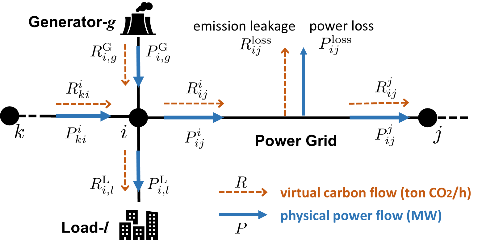
Figure 1: Illustration of virtual carbon emission flow and physical power flow.

The nodal carbon intensity of each node $i$ is calculated as (3):

$$w_{i}\!=\!\frac{R_{i}^{\mathrm{in}}}{P_{i}^{\mathrm{in}}}\!=\!\frac{\sum_{g\in\mathcal{G}_{i}}w_{i,g}^{\mathrm{G}}P_{i,g}^{\mathrm{G}}+\sum_{k\in\mathcal{N}_{i}^{+}}w_{k}P_{ki}^{i}}{\sum_{g\in\mathcal{G}_{i}}P_{i,g}^{\mathrm{G}}+\sum_{k\in\mathcal{N}_{i}^{+}}P_{ki}^{i}},\ \forall i\in\mathcal{N},$$ (3)

which is essentially the total carbon inflow divided by the total power inflow. Equation (3) indicates that the power flow and power loss of each branch $ij\in\mathcal{E}$ share the same carbon emission intensity that equals to the nodal carbon intensity of the sending node, i.e., $\frac{R_{ij}^{i}}{P_{ij}^{i}}=\frac{R_{ij}^{j}}{P_{ij}^{j}}=\frac{R_{ij}^{\mathrm{loss}}}{P_{ij}^{\mathrm{loss}}}=w_{i}$.

Equation (3) is referred to as the carbon flow model or carbon flow equation, and it can be equivalently reformulated as the matrix form (4):

$$\bm{w}_{\mathrm{N}}=(\bm{P}_{\mathrm{N}}-\bm{P}_{\mathrm{B}})^{-1}\bm{r}_{\mathrm{G}},$$ (4)

where $\bm{w}_{\mathrm{N}}\!:=\!(w_{i})_{i\in\mathcal{N}}\!\in\!\mathbb{R}^{N}$ and $\bm{r}_{\mathrm{G}}\!:=\!(\sum_{g\in\mathcal{G}_{i}}\!\!w_{i,g}^{\mathrm{G}}P_{i,g}^{\mathrm{G}})_{i\in\mathcal{N}}\!\in\!\mathbb{R}^{N}$ denote the column vectors that collect the nodal carbon intensities and nodal generation carbon flows, respectively. $\bm{P}_{\mathrm{N}}\!:=\!\text{diag}(P_{i}^{\mathrm{in}})\!\in\!\mathbb{R}^{N\times N}$ is the diagonal matrix whose $i$-th diagonal entry is the total active power inflow to node $i$. $\bm{P}_{\mathrm{B}}\!\in\!\mathbb{R}^{N\times N}$ is the power inflow matrix with $\bm{P}_{\mathrm{B}}[i,k]\!=\!P_{ki}^{i}$ and $\bm{P}_{\mathrm{B}}[k,i]\!=\!0$ if node $k$ sends power flow $P_{ki}^{i}$ to node $i$. See [6] for more explanations.

II-B Properties of Carbon Flow Matrix

We study the properties of the carbon flow matrix $\bm{P}_{\mathrm{C}}:=\bm{P}_{\mathrm{N}}-\bm{P}_{\mathrm{B}}$ below. By definition, the matrix $\bm{P}_{\mathrm{C}}$ is diagonally dominant, and we define the set $\mathcal{J}$:

$$\mathcal{J}:=\Big{\{}i\in\mathcal{N}\,\Big{\rvert}\,|\bm{P}_{\mathrm{C}}[i,i]|>\!\!\sum_{j=1;j\neq i}^{N}\!|\bm{P}_{\mathrm{C}}[i,j]|\Big{\}}.$$ (5)

In practice, $\mathcal{J}\neq\emptyset$, i.e., there exist some rows $i\in\mathcal{J}$ of $\bm{P}_{\mathrm{C}}$ that are strictly diagonally dominant; such rows correspond to the nodes with generation power injections $P_{i,g}^{\mathrm{G}}$. Then, we establish the invertibility property of $\bm{P}_{\mathrm{C}}$ with Theorem 1.

Theorem 1.

Assume that for each $i\notin\mathcal{J}$ of the matrix $\bm{P}_{\mathrm{C}}$, there is a sequence of nonzero elements of $\bm{P}_{\mathrm{C}}$ of the form $\bm{P}_{\mathrm{C}}[i,i_{1}],\bm{P}_{\mathrm{C}}[i_{1},i_{2}],\cdots,\bm{P}_{\mathrm{C}}[i_{r},j]$ with $j\in\mathcal{J}$. Then, $\bm{P}_{\mathrm{C}}$ is invertible, and $\bm{P}_{\mathrm{C}}$ is an M-matrix.

Proof.

According to [25, Theorem], the matrix $\bm{P}_{\mathrm{C}}$ is nonsingular and thus invertible. Since $\bm{P}_{\mathrm{C}}$ is diagonally dominant and all its off-diagonal elements $\{\bm{P}_{\mathrm{C}}[i,j]\}_{i\neq j}$ are non-positive, $\bm{P}_{\mathrm{C}}$ is an M-matrix [26] according to [25, Corollary 4]. ∎

Discussions. The assumption in Theorem 1 can be interpreted as that for any node $i$ with no generation power injection, one can find a power flow path $i\leftarrow i_{1}\leftarrow i_{2}\leftarrow\cdots\leftarrow i_{r}\leftarrow j$ in the power network that traces upstream to a node $j$ that has generation power injection. This assumption generally holds for practical connected power networks. This assumption also implies that every node has non-zero power flux, i.e., $\bm{P}_{\mathrm{C}}[i,i]>0$ for all $i\in[N]$. However, non-zero nodal power flux does not sufficiently guarantee that $\bm{P}_{\mathrm{C}}$ is invertible. For example, consider a simple 3-node circular network case shown in Figure 2. In this case, every node has 1 unit of power flowing through it, but the matrix $\bm{P}_{\mathrm{C}}$ is singular. Nevertheless, this case violates the assumption in Theorem 1. In addition, $\bm{P}_{\mathrm{C}}$ possesses all the properties of being an M-matrix. For example, all the elements of $\bm{P}_{\mathrm{C}}^{-1}$ are non-negative and every eigenvalue of $\bm{P}_{\mathrm{C}}$ has positive real part [26, Theorem 1.1].

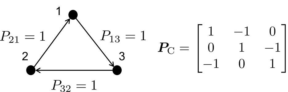
Figure 2: A simple 3-node network case example.

II-C Use of Carbon Emission Flow for Carbon Accounting

Given power flow results, one can solve the set of carbon flow equations (3) or (4) to obtain the nodal carbon intensities $\bm{w}_{\mathrm{N}}$, and then calculate all carbon flow values. Based on the carbon emission categories in the GHG Protocol [3, 2],

• Generator-$g$ at node $i$ shall account for the (Scope 1) direct carbon emission rate $R_{i,g}^{\mathrm{G}}=w_{i,g}^{\mathrm{G}}P_{i,g}^{\mathrm{G}}$;

• Load-$l$ at node $i$ shall account for the (Scope 2) attributed carbon emission rate $R_{i,l}^{\mathrm{L}}=w_{i}P_{i,l}^{\mathrm{L}}$;

• The power grid owner shall account for the (Scope 2) attributed carbon emission rate associated with the network power loss, i.e., $\sum_{ij\in\mathcal{E}}\!R_{ij}^{\mathrm{loss}}=\sum_{ij\in\mathcal{E}}\!w_{i}P_{ij}^{\mathrm{loss}}$.

The generation fuel mix and power flow change over time, leading to time-varying carbon flow profiles. In addition, the carbon emission amounts over a time period $\mathcal{T}$ (e.g., one day or one year) are the time accumulation of $R$. For example, the attributed carbon emission amount for the load-$l$ at node $i$ is calculated as $\hat{E}_{i,l,\mathcal{T}}:=\sum_{t\in\mathcal{T}}\delta_{t}w_{i,t}P_{i,l,t}^{\mathrm{L}}$, where $\delta_{t}$ is the time interval (e.g., 1 hour or 15 minutes).

III Carbon-Aware Optimal Power Flow Method

This section presents the generic C-OPF model that integrates the carbon flow model and constraints into the OPF method. Then, the reformulation and linearization techniques are introduced to tackle the modeling issues of C-OPF.

III-A Generic C-OPF Model

To enable the optimal management of carbon emissions in power system decision-making, we propose the generic C-OPF model (6) to co-optimize power flow and carbon flow.

Obj. $$\min_{\bm{x}\in\mathcal{X}}\ f_{\mathrm{power}}(\bm{x},\bm{y})+f_{\mathrm{carbon}}(\bm{x},\bm{y},\bm{z})$$ (6a)

s.t. $$\text{Power Flow Equations }(\bm{x},\bm{y})=\bm{0},$$ (6b)

$$\text{Power Flow Constraints }(\bm{y})\leq\bm{0},$$ (6c)

$$\text{Carbon Flow Equations }(\bm{x},\bm{y},\bm{z})=\bm{0},$$ (6d)

$$\text{Carbon Flow Constraints }(\bm{x},\bm{y},\bm{z})\leq\bm{0}.$$ (6e)

Here, $\bm{x}$ denotes the decision variables that are subject to the feasible set $\mathcal{X}$. The specification of $\bm{x}$ and $\mathcal{X}$ depends on the practical applications. For instance, in economic dispatch [27], $\bm{x}$ denotes the generation decisions of various generators and $\mathcal{X}$ represents the generation capacity limits and ramping constraints. $\bm{x}$ can also be the load management decisions in demand response [28], or the site and size decisions of new renewable generators in grid expansion planning [29]. $\bm{y}$ denotes the power flow-related variables, such as the network voltage profiles and branch power flows. $\bm{z}$ represents the carbon flow-related variables, such as the nodal carbon intensities $\bm{w}_{\mathrm{N}}$ and carbon flow values.

III-A1 Objective Function

The objective (6a) aims to minimize the overall cost that consists of two components: the power-related cost denoted as $f_{\mathrm{power}}$ and the carbon emission-related cost $f_{\mathrm{carbon}}$. Depending on the specific applications, $f_{\mathrm{power}}$ can be the generation cost, network loss, grid expansion investment cost, etc. $f_{\mathrm{carbon}}$ is defined to capture the externality of carbon emissions and regulatory penalty on generation-side or demand-side emissions (or the bonus on emission reduction). An example of these cost functions is given by (7):

$$f_{\mathrm{power}} :=\sum_{i\in\mathcal{N}}\sum_{g\in\mathcal{G}_{i}}\Big{(}c_{i,g}^{2}(P_{i,g}^{\mathrm{G}})^{2}+c_{i,g}^{1}{P_{i,g}^{\mathrm{G}}}+c_{i,g}^{0}\Big{)},$$ (7a)

$$f_{\mathrm{carbon}} :=c^{\mathrm{emi}}\cdot\sum_{i\in\mathcal{N}}\sum_{g\in\mathcal{G}_{i}}{w_{i,g}^{\mathrm{G}}}{P_{i,g}^{\mathrm{G}}},$$ (7b)

where (7a) denotes the total generation cost in a quadratic form with the parameters $c_{i,g}^{2},c_{i,g}^{2},c_{i,g}^{0}$, and (7b) is the penalty on generation-side emissions with the cost coefficient $c^{\mathrm{emi}}$.

III-A2 Power Flow Equations and Constraints

The power flow equations (6b) and power flow constraints (6c) remain the same as them in classic OPF models [30, 5, 4]. The full power flow equations (6b) can be formulated as (8):

$$P_{ij}^{i}=(V_{i}^{2}-V_{i}V_{j}\cos(\theta_{i}-\theta_{j}))g_{ij}$$

$$\qquad\qquad\qquad-V_{i}V_{j}\sin(\theta_{i}-\theta_{j})b_{ij}, \forall ij\in\mathcal{E},$$ (8a)

$$Q_{ij}^{i}=(V_{i}V_{j}\cos(\theta_{i}-\theta_{j})-V_{i}^{2})b_{ij}$$

$$\qquad\qquad\qquad-V_{i}V_{j}\sin(\theta_{i}-\theta_{j})g_{ij}, \forall ij\in\mathcal{E},$$ (8b)

$$\sum_{j\in\mathcal{N}_{i}}P_{ij}^{i}\,=\sum_{g\in\mathcal{G}_{i}}P_{i,g}^{\mathrm{G}}-\sum_{l\in\mathcal{L}_{i}}P_{i,l}^{\mathrm{L}}, \forall i\in\mathcal{N},$$ (8c)

$$\sum_{j\in\mathcal{N}_{i}}Q_{ij}^{i}=\sum_{g\in\mathcal{G}_{i}}Q_{i,g}^{\mathrm{G}}-\sum_{l\in\mathcal{L}_{i}}Q_{i,l}^{\mathrm{L}}, \forall i\in\mathcal{N},$$ (8d)

where $V_{i}$ and $\theta_{i}$ are the voltage magnitude and phase angle at node $i$. $Q_{ij}^{i}$ denotes the reactive power flow of branch $ij$ from node $i$ to node $j$ measured at node $i$. $g_{ij}$ and $b_{ij}$ are the conductance and susceptance of branch $ij$.

The power flow constraints (6c) generally involve the line thermal constraints (9a) and voltage limits (9b).

$$\qquad-\bar{P}_{ij}\leq \,P_{ij}^{i}\leq\bar{P}_{ij}, \forall ij\in\mathcal{E},$$ (9a)

$$\qquad\underline{V}_{i}\leq \,V_{i}\leq\bar{V}_{i}, \forall i\in\mathcal{N},$$ (9b)

where $\bar{P}_{ij}$ is the line thermal capacity, and $\bar{V}_{i},\underline{V}_{i}$ are the upper and lower limits of voltage magnitude at node $i$.

Since the power flow equations and constraints remain the same, the linearization or convexification methods developed for them are still applicable. For instance, the classic DC power flow model (10) [30] can be used in the C-OPF model to replace the complete power flow equations (8) for simplicity. In (10a), the superscript “$i$” is omitted since $P_{ij}^{i}=P_{ij}^{j}$ in the DC power flow model due to neglecting power loss.

$$P_{ij}=-b_{ij}\cdot(\theta_{i}-\theta_{j}), \forall ij\in\mathcal{E},$$ (10a)

$$\text{Equation }\eqref{eq:full:p}.$$ (10b)

III-A3 Carbon Flow Equations and Constraints

The carbon flow equations (6d) are given by (III-A3):

$$w_{i} \big{(}\sum_{g\in\mathcal{G}_{i}}\!P_{i,g}^{\mathrm{G}}+\sum_{j\in\mathcal{N}_{i}^{+}}\!\!P_{ji}^{i}\big{)}$$

$$\qquad=\!\sum_{g\in\mathcal{G}_{i}}\!w_{i,g}^{\mathrm{G}}P_{i,g}^{\mathrm{G}}+\!\!\sum_{j\in\mathcal{N}_{i}^{+}}\!\!\!w_{j}P_{ji}^{i},\qquad\forall i\in\mathcal{N},$$ (11)

which is simply an equivalent reformulation of (3).

The carbon flow constraints (6e) can take various forms depending on practical requirements. For example, an upper limit $\bar{\bm{w}}_{\mathrm{N}}:=(\bar{w}_{i})_{i\in\mathcal{N}}$ can be imposed on the nodal carbon intensities, i.e. (12), to ensure that the users at these nodes are supplied with low-carbon electricity. By adjusting this upper limit $\bar{\bm{w}}_{\mathrm{N}}$, one can control the level of “cleanness” of the supplied electricity at a certain location. In particular, letting $\bar{w}_{i}=0$ enforces that the electricity supply at node $i$ is completely carbon-free. We note that the definition of “node” can vary in terms of geographical scales, which can represent a district grid, a distribution feeder, or a balancing area.

$$\qquad\qquad w_{i} \leq\bar{w}_{i}, \forall i\in\mathcal{N}.$$ (12)

An alternative carbon flow constraint (6e) can impose a cap $\bar{R}_{i,l}^{\mathrm{L}}$ on individual user-side carbon emissions as (13):

$$\qquad\qquad w_{i}\cdot P_{i,l}^{\mathrm{L}} \leq\bar{R}_{i,l}^{\mathrm{L}}, \forall l\in\mathcal{L}_{i},i\in\mathcal{N}.$$ (13)

Besides, instead of an emission cap on individual users, a cap $\bar{R}_{i}^{\mathrm{L}}$ on the nodal level emissions can be imposed as (14):

$$\qquad\qquad w_{i}\cdot\big{(}\sum_{l\in\mathcal{L}_{i}}P_{i,l}^{\mathrm{L}}\big{)} \leq\bar{R}_{i}^{\mathrm{L}}, \forall i\in\mathcal{N}.$$ (14)

When the loads $P_{i,l}^{\mathrm{L}}$ are given parameters rather than variables, constraints (13) and (14) are equivalent to (12) by letting $\bar{w}_{i}=\min_{l\in\mathcal{L}_{i}}\bar{R}_{i,l}^{\mathrm{L}}/P_{i,l}^{\mathrm{L}}$ and $\bar{w}_{i}=\bar{R}_{i}^{\mathrm{L}}/(\sum_{l\in\mathcal{L}_{i}}\!P_{i,l}^{\mathrm{L}})$. Other carbon flow constraints, such as the requirement on carbon emissions fairness and equity [12], can also be employed.

Remark 1.

Due to the propositional sharing principle in the carbon flow model, a natural limit on nodal carbon intensities is that $w_{i}\in[0,w^{\mathrm{G}}_{\max}]$ for all $i\in\mathcal{N}$, where $w_{\max}^{\mathrm{G}}:=\max_{i,g}\{w_{i,g}^{\mathrm{G}}\}$ is the largest generation carbon emission factor. Hence, if we set $\bar{w}_{i}$ in (12) to be larger than $w_{\max}^{\mathrm{G}}$ for some nodes $i$, (12) imposes no actual constraint on these nodes.

Another critical issue is that if the carbon flow constraints are not appropriately designed, they may render the C-OPF model (6) infeasible, e.g., when the caps in (12)-(14) are too small to be achievable. To address this issue, the hard constraints (12)-(14) can be converted to be soft constraints by adding slack variables with corresponding penalties in the objective. For example, one can replace constraint (14) with (15) and add a penalty term $\sum_{i\in\mathcal{N}}(c_{i}^{\mathrm{R}}\cdot\tilde{R}_{i}^{\mathrm{L}})$ to the carbon-related cost function $f_{\mathrm{carbon}}$ in objective (6a):

$$\quad w_{i}\cdot\big{(}\sum_{l\in\mathcal{L}_{i}}P_{i,l}^{\mathrm{L}}\big{)} \leq\bar{R}_{i}^{\mathrm{L}}+\tilde{R}_{i}^{\mathrm{L}},\ \ \tilde{R}_{i}^{\mathrm{L}}\geq 0, \forall i\in\mathcal{N},$$ (15)

where $\tilde{R}_{i}^{\mathrm{L}}$ is the slack variable and $c_{i}^{\mathrm{R}}$ denotes the penalty cost coefficient for excessive demand-side emissions. ∎

Essentially, the C-OPF model (6) is a generalization of the OPF method, and it reduces to an OPF model if the carbon-related objective function $f_{\mathrm{carbon}}$, carbon flow equations (6d) and constraints (6e) are removed or inactive. It also implies that existing OPF techniques, such as linearization, convexification, decomposition, stochastic modeling, etc., can still be applied to the power flow components in C-OPF (6). Moreover, the C-OPF model (6) naturally extends to the multi-time period setting with time-coupling constraints.

III-B Reformulation for Power Flow Directions

As mentioned in the introduction section and indicated by the set $\mathcal{N}_{i}^{+}$, the carbon flow equation $\eqref{eq:mcieq}$ requires the pre-determination of branch power flow directions to identify the power inflows for each node. However, the directions of branch power flows are generally unknown prior to solving the C-OPF problem. To address this issue, we introduce two non-negative power flow variables $\hat{P}_{ji}^{i}\!\geq\!0$ and $\hat{P}_{ij}^{i}\!\geq\!0$ for each branch $ij\in\mathcal{E}$ with $P_{ij}^{i}=\hat{P}_{ij}^{i}-\hat{P}_{ji}^{i}$. Specifically, $\hat{P}_{ji}^{i}$ and $\hat{P}_{ij}^{i}$ denote the power flow components from node $j$ to node $i$ and from node $i$ to node $j$, respectively, both of which are measured on the side of node $i$. Then, we can equivalently reformulate the carbon flow equation (III-A3) as (16), and also need to replace $P_{ij}^{i}$ with $\hat{P}_{ij}^{i}-\hat{P}_{ji}^{i}$ in the power flow equations (8) (or the DC power flow model (10)) and constraints (9a).

$$w_{i}(\sum_{g\in\mathcal{G}_{i}}\!P_{i,g}^{\mathrm{G}}+\!\sum_{j\in\mathcal{N}_{i}}\!\hat{P}_{ji}^{i})$$

$$\qquad=\sum_{g\in\mathcal{G}_{i}}\!\!w_{i,g}^{\mathrm{G}}P_{i,g}^{\mathrm{G}}+\!\!\sum_{j\in\mathcal{N}_{i}}\!\!\!w_{j}\hat{P}_{ji}^{i}, \forall i\in\mathcal{N}$$ (16a)

$$\hat{P}_{ji}^{i}\geq 0,\ \hat{P}_{ij}^{i}\geq 0, \forall ij\in\mathcal{E}$$ (16b)

$$\hat{P}_{ji}^{i}\cdot\hat{P}_{ij}^{i}=0, \forall ij\in\mathcal{E}.$$ (16c)

In (16a), we replace $\mathcal{N}_{i}^{+}$ (the set of neighbor nodes that send power to node $i$) by $\mathcal{N}_{i}$ (the set of all neighbor nodes of node $i$). In addition, the complementarity constraint (16c) is added to ensure either $\hat{P}_{ji}^{i}$ or $\hat{P}_{ij}^{i}$ must be zero for each branch $ij$. Here, a useful trick to facilitate the nonlinear optimization is to replace the complementarity constraint (16c) by the relaxed constraint (17) [31], and this relaxation is exact due to (16b).

$$\qquad\hat{P}_{ji}^{i}\cdot\hat{P}_{ij}^{i}\leq 0,\qquad\forall ij\in\mathcal{E}.$$ (17)

Alternatively, we can introduce a binary variable $\gamma_{ij}$ for $ij\in\mathcal{E}$ and replace the complementarity constraint (16c) by

$$\gamma_{ij}\in\{0,1\},\ \hat{P}_{ji}^{i}\leq(1-\gamma_{ij})\bar{P}_{ij},\ \hat{P}_{ij}^{i}\leq\gamma_{ij}\bar{P}_{ij}.$$ (18)

Note that both reformulations via (16) or (18) are equivalent to the original carbon flow equation (III-A3), but they do not need to know the branch flow directions in advance.

III-C Linearization to Handle Bilinear Terms

In the C-OPF model, the generation power $P_{i,g}^{\mathrm{G}}$, power flow $P_{ji}^{i}$, and nodal carbon intensities $w_{i}$ are typically variables. Therefore, there are many bilinear terms in the carbon flow equations (III-A3) (or (16a)), such as $w_{i}P_{ji}^{i}$ and $w_{i}P_{i,g}^{\mathrm{G}}$, making the C-OPF model nonlinear and nonconvex. In this subsection, we present inner and outer linearization approaches to handle these bilinear terms.

III-C1 Inner Linearization Method

Consider the case when the carbon flow constraints (6e) take the form of (12), i.e., $\bm{w}_{\mathrm{N}}\leq\bar{\bm{w}}_{\mathrm{N}}$. As mentioned above, carbon flow constraints (13) and (14) can also be reformulated as (12) when the loads $P_{i,l}^{\mathrm{L}}$ are given parameters. Recall that the carbon flow equations (III-A3) can be written as the matrix form (4). Then, one can eliminate the nodal carbon intensity variable $\bm{w}_{\mathrm{N}}$ and equivalently reformulate the carbon flow equations (III-A3) and constraints (12) as (19):

$$(\bm{P}_{\mathrm{N}}-\bm{P}_{\mathrm{B}})^{-1}\bm{r}_{\mathrm{G}}\leq\bar{\bm{w}}_{\mathrm{N}}.$$ (19)

Constraint (19) is generally nonlinear and nonconvex due to the matrix inverse. It motivates us to multiply $\bm{P}_{\mathrm{N}}-\bm{P}_{\mathrm{B}}$ to both sides of (19) and results in a new constraint (20):

$$\bm{r}_{\mathrm{G}}\leq(\bm{P}_{\mathrm{N}}-\bm{P}_{\mathrm{B}})\bar{\bm{w}}_{\mathrm{N}},$$ (20)

which represents a set of linear constraints on the power flow variables. In addition, we have the following proposition on the relation between (19) and (20).

Proposition 1.

Suppose that the assumption in Theorem 1 holds. In terms of the feasible set $\mathcal{F}_{1}$ defined as (21) and the feasible set $\mathcal{F}_{2}$ defined as (22), we have $\mathcal{F}_{2}\subseteq\mathcal{F}_{1}$.

$$\mathcal{F}_{1} :=\big{\{}(\bm{r}_{\mathrm{G}},\bm{P}_{\mathrm{N}},\bm{P}_{\mathrm{B}})|\text{ Constraint \eqref{eq:combine1}}\,\big{\}},$$ (21)

$$\mathcal{F}_{2} :=\big{\{}(\bm{r}_{\mathrm{G}},\bm{P}_{\mathrm{N}},\bm{P}_{\mathrm{B}})|\text{ Constraint \eqref{eq:combine2}}\,\big{\}}.$$ (22)

Proof.

For any solution $(\bm{r}_{\mathrm{G}},\bm{P}_{\mathrm{N}},\bm{P}_{\mathrm{B}})$ that satisfies (20), we have $\bm{r}_{\mathrm{G}}-(\bm{P}_{\mathrm{N}}-\bm{P}_{\mathrm{B}})\bar{\bm{w}}_{\mathrm{N}}\leq 0$, and we multiply both sides by $(\bm{P}_{\mathrm{N}}-\bm{P}_{\mathrm{B}})^{-1}$. Since all elements of $(\bm{P}_{\mathrm{N}}-\bm{P}_{\mathrm{B}})^{-1}$ are non-negative according to Theorem 1, it leads to (19). Therefore, any $(\bm{r}_{\mathrm{G}},\bm{P}_{\mathrm{N}},\bm{P}_{\mathrm{B}})$ that satisfies (20) must satisfy (19). ∎

Proposition 1 indicates that the linear constraint (20) is an inner approximation to the original nonlinear constraint (19). Hence, any solutions that satisfy (20) must be feasible for (19), and replacing (19) with (20) in the C-OPF model provides an upper bound of the original optimal objective value.

III-C2 Outer Linearization Method

In addition to the proposed linearization method above, which leverages a special property of the carbon flow model, there are many other general linearization and relaxation techniques [32, 33] that can be employed to handle the bilinear terms. One such well-known approach is the McCormick envelope method [32] that replaces each bilinear term with a new variable and a set of relaxed linear constraints. For example, considering the bilinear term $w_{i}P_{i,g}^{G}$ with the given lower and upper bounds $w_{i}\in[\underline{w}_{i},\bar{w}_{i}]$ and $P_{i,g}^{G}\in[\underline{P}_{i,g}^{G},\bar{P}_{i,g}^{G}]$, one can define a new variable $y_{i,g}=w_{i}P_{i,g}^{G}$ to replace it and add the following linear constraints (23):

$$y_{i,g} \geq\underline{P}_{i,g}^{G}w_{i}+\underline{w}_{i}{P}_{i,g}^{G}-\underline{w}_{i}\underline{P}_{i,g}^{G},$$ (23a)

$$y_{i,g} \geq\bar{P}_{i,g}^{G}w_{i}+\bar{w}_{i}{P}_{i,g}^{G}-\bar{w}_{i}\bar{P}_{i,g}^{G},$$ (23b)

$$y_{i,g} \leq\underline{P}_{i,g}^{G}w_{i}+\bar{w}_{i}{P}_{i,g}^{G}-\bar{w}_{i}\underline{P}_{i,g}^{G},$$ (23c)

$$y_{i,g} \leq\bar{P}_{i,g}^{G}w_{i}+\underline{w}_{i}{P}_{i,g}^{G}-\underline{w}_{i}\bar{P}_{i,g}^{G}.$$ (23d)

The McCormick envelope method provides linear relaxation of the bilinear terms and results in a lower bound of the original optimal objective value. The relaxation gap depends on the tightness of the given lower and upper bounds. Moreover, piecewise McCormick relaxation can be used to further tighten the relaxation; see [34, 33] for details.

When the proposed binary reformulation (18) and linearization methods above are adopted, together with linearized power flow equations and objective function, the C-OPF model (6) becomes a mixed integer linear programming (MILP) problem, which can be solved via many available optimizers, such as Gurobi and IBM CPLEX. Otherwise, nonlinear optimizers, such as Ipopt [35], can be used to solve the C-OPF model.

IV Carbon Emission Model for Energy Storage

Energy storage (ES) systems play an important role in power system decarbonization, as they can charge when the grid is mainly supplied by renewable generation and discharge when the grid relies on high-emission generation sources. In this section, we develop two carbon emission models as well as carbon accounting methods for ES systems.

Consider that an ES system is connected to node $i\!\in\!\mathcal{N}$. For time $t\in\mathcal{T}:=\{1,2,\cdots,T\}$ with the time interval $\delta_{t}$, the dynamic ES power model [36] is formulated as (24):

$$0\leq P_{i,t}^{\mathrm{ch}}\leq\bar{P}_{i}^{\mathrm{ch}},\ \ 0\leq P_{i,t}^{\mathrm{dc}}\leq\bar{P}_{i}^{\mathrm{dc}},$$ (24a)

$$P_{i,t}^{\mathrm{ch}}\cdot P_{i,t}^{\mathrm{dc}}=0,$$ (24b)

$$e_{i,t+1}^{\mathrm{es}}=\kappa_{i}e_{i,t}^{\mathrm{es}}+\delta_{t}\big{(}\eta_{i}^{\mathrm{ch}}P_{i,t}^{\mathrm{ch}}-\frac{1}{\eta_{i}^{\mathrm{dc}}}P_{i,t}^{\mathrm{dc}}\big{)},$$ (24c)

$$\underline{e}_{i}\leq e_{i,t}^{\mathrm{es}}\leq\bar{e}_{i},\quad e_{i,T+1}^{\mathrm{es}}=e_{i,1}^{\mathrm{es}},\quad\forall i\in\mathcal{N},t\in\mathcal{T}.$$ (24d)

Here, $\bar{P}_{i}^{\mathrm{ch}}$ and $\bar{P}_{i}^{\mathrm{dc}}$ are the charging and discharging power capacities. $\eta_{i}^{\mathrm{ch}}\!\in\!(0,1]$ and $\eta_{i}^{\mathrm{dc}}\!\in\!(0,1]$ denote the charging and discharging efficiency coefficients, respectively. $\kappa_{i}\!\in\!(0,1]$ denotes the storage efficiency factor that models the loss of stored energy over time. $\bar{e}_{i}$ and $\underline{e}_{i}$ are the upper and lower bounds of the energy level of the ES system. The complementarity constraint (24b) is used to enforce that an ES unit can not charge and discharge at the same time.

Below, we develop two carbon emission models for ES systems: the “water tank” model and the “load/carbon-free generator” model. We also present the corresponding carbon accounting schemes for ES owners based on these models.

IV-A “Water Tank” Carbon Emission Model

The “water tank” model is conceptually consistent with the analogy of “water flow” used to explain the carbon flow model in Section II-A. Analogous to a water tank that stores both water and invisible particles, an ES system is viewed to store both electric energy $e_{i,t}^{\mathrm{es}}$ (in the unit of MWh) and virtual carbon emissions $E_{i,t}^{\mathrm{es}}$ (in the unit of ton$\mathrm{CO_{2}}$). We then define the internal ES carbon intensity $w_{i,t}^{\mathrm{es}}$ as (25):

$$w_{i,t}^{\mathrm{es}}=E_{i,t}^{\mathrm{es}}/e_{i,t}^{\mathrm{es}}.$$ (25)

Note that $e_{i,t}^{\mathrm{es}}$ should not be zero to make $w_{i,t}^{\mathrm{es}}$ well-defined. This can be achieved by setting the lower energy bound $\underline{e}_{i}$ in (24d) to be a small positive value rather than zero. It can also prevent the numerical issues that may arise during the optimization process.

Based on the ES power model (24), we develop the dynamic carbon emission model of ES as (26) for $t\in\mathcal{T}$:

$$E_{i,t+1}^{\mathrm{es}}=\kappa_{i}E_{i,t}^{\mathrm{es}}+\delta_{t}\big{(}w_{i,t}\eta_{i}^{\mathrm{ch}}P_{i,t}^{\mathrm{ch}}-w_{i,t}^{\mathrm{es}}\frac{1}{\eta_{i}^{\mathrm{dc}}}P_{i,t}^{\mathrm{dc}}\big{)}.$$ (26)

Model (26) implies that (virtual) carbon emissions are injected into the ES unit when it charges with the electricity in the nodal carbon intensity $w_{i,t}$; and it releases the stored emissions back to the grid when it discharges with the electricity in the ES carbon intensity $w_{i,t}^{\mathrm{es}}$. In particular, (26) models the carbon emission leakage associated with the energy loss during the storage, charging, and discharging processes of the ES unit, as shown in Figure 3.

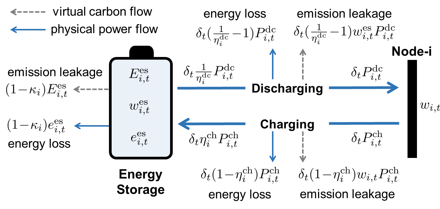
Figure 3: Power flow and carbon flow under the “water tank” ES model.

Alternatively, we can plug in the ES carbon intensity (25) into (26) to eliminate the variable $E_{i,t}^{\mathrm{es}}$ and reformulate the ES carbon emission model equivalently as (27):

$$w_{i,t+1}^{\mathrm{es}}\!=\!\frac{\kappa_{i}e_{i,t}^{\mathrm{es}}}{\kappa_{i}e_{i,t}^{\mathrm{es}}\!+\!\delta_{t}\eta_{i}^{\mathrm{ch}}P_{i,t}^{\mathrm{ch}}}\cdot w_{i,t}^{\mathrm{es}}\!+\!\frac{\delta_{t}\eta_{i}^{\mathrm{ch}}P_{i,t}^{\mathrm{ch}}}{\kappa_{i}e_{i,t}^{\mathrm{es}}\!+\!\delta_{t}\eta_{i}^{\mathrm{ch}}P_{i,t}^{\mathrm{ch}}}\cdot w_{i,t},$$ (27)

which describes the dynamics of the ES carbon intensity $w_{i,t}^{{\mathrm{es}}}$ and is the alternate form of the proposed ES carbon emission model. An intuitive property of this model (27) is:

• When discharging, the ES carbon intensity remains unchanged with $w_{i,t+1}^{\mathrm{es}}=w_{i,t}^{\mathrm{es}}$;

• When charging, the ES carbon intensity at the next time $w_{i,t+1}^{\mathrm{es}}$ is a convex combination of the current ES carbon intensity $w_{i,t}^{\mathrm{es}}$ and the nodal carbon intensity $w_{i,t}$ with the weight coefficient $\frac{\kappa_{i}e_{i,t}^{\mathrm{es}}}{\kappa_{i}e_{i,t}^{\mathrm{es}}\!+\!\delta_{t}\eta_{i}^{\mathrm{ch}}P_{i,t}^{\mathrm{ch}}}\in(0,1)$.

Accordingly, the carbon flow equation (16a) in the C-OPF model is modified as (IV-A) to integrate the ES system.

$$w_{i,t}\big{(}P_{i,t}^{\mathrm{dc}}+\sum_{g\in\mathcal{G}_{i}}\!\!P_{i,g,t}^{\mathrm{G}}+\!\!\!\sum_{j\in\mathcal{N}_{i}}\!\!\!\hat{P}_{ji,t}^{i}\big{)}=w_{i,t}^{\mathrm{es}}P_{i,t}^{\mathrm{dc}}$$

$$\quad+\!\sum_{g\in\mathcal{G}_{i}}\!\!w_{i,g,t}^{\mathrm{G}}P_{i,g,t}^{\mathrm{G}}+\!\!\sum_{j\in\mathcal{N}_{i}}\!\!\!w_{j,t}\hat{P}_{ji,t}^{i},\quad\forall i\in\mathcal{N},t\in\mathcal{T}.$$ (28)

From (IV-A), it is seen that an ES unit affects the nodal carbon intensities and carbon flow only when it discharges.

Remark 2.

(Carbon Accounting for ES Owner). Under the “water tank” carbon emission model, for the time period $\mathcal{T}$, the owner of the ES unit shall account for the (Scope 2) attributed carbon emission $\hat{E}_{i,\mathcal{T}}^{\mathrm{es}}$ calculated by (29):

$$\quad\hat{E}_{i,\mathcal{T}}^{\mathrm{es}}=\sum_{t=1}^{T}\delta_{t}(w_{i,t}P_{i,t}^{\mathrm{ch}}-w_{i,t}^{\mathrm{es}}P_{i,t}^{\mathrm{dc}}),\quad\forall i\in\mathcal{N},$$ (29)

which is the net carbon emissions withdrawn from the grid. Intuitively, the attributed carbon emissions $\hat{E}_{i,\mathcal{T}}^{\mathrm{es}}$ can be interpreted as two components: 1) the change of virtually stored carbon emissions, i.e., $E_{i,T+1}^{\mathrm{es}}\!-\!E_{i,1}^{\mathrm{es}}$, and 2) the carbon emission leakage associated with ES energy loss during storage, charging, and discharging, i.e., $E_{i,1}^{\mathrm{es}}+\sum_{t=1}^{T}\delta_{t}(w_{i,t}P_{i,t}^{\mathrm{ch}}-w_{i,t}^{\mathrm{es}}P_{i,t}^{\mathrm{dc}})-E_{i,T+1}^{\mathrm{es}}$. To make it more clear, we consider a lossless ES unit with $\kappa_{i}\!=\!\eta_{i}^{\mathrm{ch}}\!=\!\eta_{i}^{\mathrm{dc}}\!=\!1$. If this ES unit recovers the initially stored emission level in the final time step, namely $E_{i,T+1}^{\mathrm{es}}\!=\!E_{i,1}^{\mathrm{es}}$, we have $\hat{E}_{i,\mathcal{T}}^{\mathrm{es}}=E_{i,T+1}^{\mathrm{es}}-E_{i,1}^{\mathrm{es}}=0$ from (26). It implies that in this case, the ES owner accounts for zero carbon emissions, regardless of the number of charging and discharging cycles during the time period $\mathcal{T}$. This outcome aligns with the role of an ES system, which does not directly produce or consume electricity (carbon emissions) itself but rather enables the temporal shifts. ∎

Remark 3.

(Comparison with Existing ES Carbon Emission Models). Similar to the “water tank” model, existing carbon emissions models for ES systems [18, 17, 24] formulate the dynamics of virtually stored emissions. However, these models do not consider the carbon emission leakage associated with energy loss during ES operation. This issue renders the ES carbon emission models not rigorous or even problematic. For instance, consider an ES unit that stays unused, i.e., neither charging nor discharging. As time passes, its stored energy $e_{t}$ gradually diminishes to zero. If the emission leakage associated with the energy loss is neglected, its virtually stored carbon emission $E_{t}$ remains constant. Consequently, the internal carbon intensity $E_{t}/e_{t}$ of the ES unit would tend towards an infinitely large value. Moreover, to ensure the credibility of carbon accounting, the attribution of carbon emissions should be consistent with where the energy goes. ∎

IV-B “Load/Carbon-Free Generator” Carbon Emission Model

The proposed “water tank” model and other existing ES carbon emission models [18, 17, 24] maintain a dynamic tracking of the virtually stored carbon emissions, which may be arduous to apply in practice. To this end, we propose the “load/carbon-free generator” model to characterize the carbon emissions of ES systems. This model treats an ES unit as a load when charging and as a carbon-free clean generator when discharging. Thus, this “load/carbon-free generator” model does not need to model ES carbon emission dynamics, and it is straightforward and easy to implement. Accordingly, the carbon flow equation (16a) in the C-OPF model is modified as (IV-A) with $w_{i,t}^{\mathrm{es}}\equiv 0$, as the ES unit is regarded as a carbon-free generator during discharging.

Under the “load/carbon-free generator” model, for the time period $\mathcal{T}$, the owner of the ES unit shall account for the (Scope 2) attributed carbon emissions $\hat{E}_{i,\mathcal{T}}^{\mathrm{es}}$ calculated by (30):

$$\hat{E}_{i,\mathcal{T}}^{\mathrm{es}}=\sum_{t=1}^{T}\delta_{t}w_{i,t}P_{i,t}^{\mathrm{ch}},\qquad\forall i\in\mathcal{N}.$$ (30)

It implies that the virtual carbon emissions absorbed from the grid during the charging period accumulate locally at the ES unit and are not released back to the grid. Thus, the ES owner bears more Scope-2 carbon emissions compared with the carbon accounting scheme (29) in the “water tank” model. Nevertheless, under the “load/carbon-free generator” model, ES owners can make profits by acting as clean energy suppliers in the carbon-electricity market, e.g., selling renewable energy certificates (RECs) [37], since the ES discharging power is considered carbon-free. As a result, ES owners are incentivized to charge their units when the grid is “clean” with low carbon emission intensities, to reduce their own carbon emissions inventories (30); and they are incentivized to discharge when the grid is in a high emission status to make more profit, as the price of clean electricity or RECs is expected to be higher at that time. In this way, the “load/carbon-free generator” scheme is easy to use in practice and naturally incentivizes the low-carbon operation of ES systems.

Besides the two proposed carbon emission models for ES systems, alternative valid models can also be employed. The use of different carbon emission models may yield discrepancies in carbon accounting outcomes, operational decision-making, and market design for ES. Hence, it is crucial to assess the impact and select an appropriate ES emission model that aligns with the practical objectives and requirements.

V Numerical Experiments

In this section, we build a carbon-aware economic dispatch model based on the C-OPF method as an example for numerical tests. We compare the simulation results with OPF-based economic dispatch schemes.

Figure 4: The modified 39-bus New England test system.

V-A Carbon-Aware Economic Dispatch and Test Settings

Based on the C-OPF method (6), we develop the carbon-aware economic dispatch (C-ED) model (31) for $t\in\mathcal{T}:=\{1,2,\cdots,T\}$ as an application example. It involves the multi-period optimal power scheduling of various generators and ES systems. The C-ED model (31) is formulated as a nonlinear optimization and we solve it using the Ipopt optimizer [35].

Obj. $$\ \min\sum_{i\in\mathcal{N}}\sum_{t\in\mathcal{T}}\Big{[}\sum_{g\in\mathcal{G}_{i}}\!\big{(}c_{i,g}^{2}(P_{i,g,t}^{\mathrm{G}})^{2}+c_{i,g}^{1}{P_{i,g,t}^{\mathrm{G}}}+c_{i,g}^{0}\big{)}$$

$$\qquad\qquad\qquad\quad+c_{i}^{\mathrm{es}}(P_{i,t}^{\mathrm{dc}}+P_{i,t}^{\mathrm{ch}})\Big{]},$$ (31a)

s.t. $$\underline{P}_{i,g,t}^{\mathrm{G}}\leq{P}_{i,g,t}^{\mathrm{G}}\leq\bar{P}_{i,g,t}^{\mathrm{G}}, \forall i\!\in\!\mathcal{N},g\!\in\!\mathcal{G}_{i},$$ (31b)

$$\underline{\Delta}_{i,g}^{\mathrm{G}}\leq{P}_{i,g,t}^{\mathrm{G}}\!-\!{P}_{i,g,t\!-\!1}^{\mathrm{G}}\leq\bar{\Delta}_{i,g}^{\mathrm{G}}, \forall i\!\in\!\mathcal{N},g\!\in\!\mathcal{G}_{i},$$ (31c)

$$\hat{P}_{ij,t}-\hat{P}_{ji,t}=-b_{ij}\cdot(\theta_{i,t}-\theta_{i,j}), \hskip 11.0pt\forall ij\!\in\!\mathcal{E},$$ (31d)

$$\sum_{j\in\mathcal{N}_{i}}(\hat{P}_{ij,t}-\hat{P}_{ji,t})=\sum_{g\in\mathcal{G}_{i}}P_{i,g,t}^{\mathrm{G}}$$

$$\qquad\qquad\quad-P_{i,t}^{\mathrm{L}}+P_{i,t}^{\mathrm{dc}}-P_{i,t}^{\mathrm{ch}}, \hskip 11.0pt\forall i\!\in\!\mathcal{N},$$ (31e)

$$0\leq\hat{P}_{ij,t}\leq\bar{P}_{ij},\ 0\leq\hat{P}_{ji,t}\leq\bar{P}_{ij}, \hskip 11.0pt\forall ij\!\in\!\mathcal{E},$$ (31f)

$$\hat{P}_{ij,t}\cdot\hat{P}_{ji,t}\leq 0, \hskip 11.0pt\forall ij\!\in\!\mathcal{E},$$ (31g)

$$w_{i,t}\leq\bar{w}_{i,t}, \hskip 11.0pt\forall i\!\in\!\mathcal{N},$$ (31h)

$$\text{Equations \eqref{eq:ESpower} \eqref{eq:ES:dyn2} \eqref{eq:cf:ES1}}.$$ (31i)

Equations (31b) and (31c) are the generation capacity and ramping constraints for various generators. Constraints (31d)-(31g) represents the DC power flow equations and line thermal limits using the bi-directional power flow model introduced in Section III-B. Equation (31h) is the carbon flow constraint that imposes a cap on the nodal carbon intensities; it enables the active management of nodal carbon intensities and ensures that the utilities supply clean power to users with a carbon intensity no greater than $\bar{w}_{i,t}$. Equations (31i) include the energy model and the “water tank” carbon emission model of ES systems, as well as the carbon flow equations. The objective (31a) consists of the generation cost and the degradation cost of ES systems. As a comparison, the OPF-based ED model is a reduced version of the C-ED model (31) which removes the carbon-related constraints (31h) (27) (IV-A) and does not need to model the bi-directional power flow variables. We solve the OPF-based ED model using the Gurobi optimizer [38].

In the simulations, we consider day-ahead economic dispatch with $T=12$ time steps and 2-hour intervals. The modified 39-bus New England system, as shown in Figure 4, is used as the test system, which includes 3 coal power plants, 3 natural gas power plants, 2 wind farms, 2 solar farms, 3 ES systems, and 21 loads. The generation carbon emission factors $w_{i,g}^{\mathrm{G}}$ are 2.26, 0.97, and 0 (lbs/kWh) for coal plants, natural gas plants, and renewable generators, respectively. The carbon flow constraint (31h) is imposed for all the load nodes and all $t\in\mathcal{T}$, and we set the cap $\bar{w}_{i,t}=1.2$ lbs/kWh. Other detailed system parameters and settings are provided in [39].

V-B Simulation Results

As illustrated in Figure 5, simulation results show that the C-OPF-based C-ED model (31) can generate effective power dispatch schemes that maintain the nodal carbon intensities of load nodes below the upper bound $\bar{w}_{i,t}=1.2$ lbs/kWh. Figure 6 shows the total generation-side and attributed load-side carbon emission rates over time. Differences between the generation-side and load-side emissions at each time $t$ are caused by the operation of ES systems. The time-varying energy level $e_{i,t}^{\mathrm{es}}$ and virtually stored carbon emissions $E_{i,t}^{\mathrm{es}}$ of the ES system at node-38 are shown in Figure 7.

TABLE I: Operational Cost of OPF-based and C-OPF-based ED schemes.

Cost (k$)	Coal	Natural Gas	Renewable	Energy Storage	Total
OPF	4414.3	6322.3	50.7	15.5	10802.8
C-OPF	1551.9	10977.7	50.7	23.3	12603.6

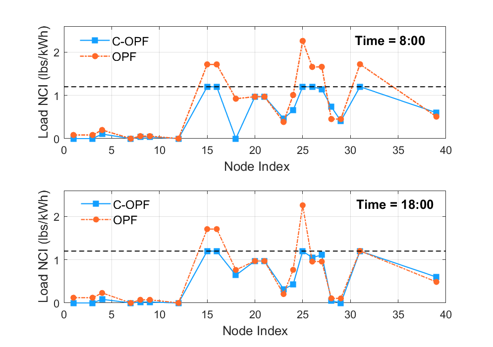
Figure 5: The nodal carbon intensities (NCI) for load nodes under C-OPF-based and OPF-based economic dispatch schemes at 8:00 and 18:00.

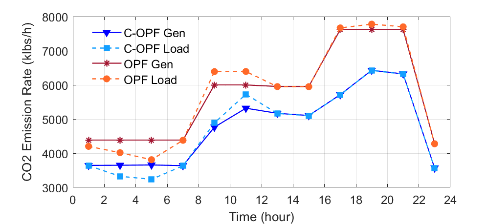
Figure 6: The total (Scope 1) generation-side carbon emission rate and the total (Scope 2) attributed load-side carbon emission rate over time under the C-OPF-based and OPF-based economic dispatch schemes.

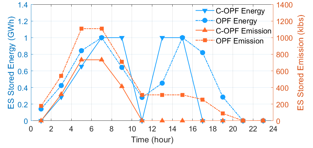
Figure 7: The stored energy and virtual carbon emissions of the ES system at node-38 under the C-OPF-based and OPF-based economic dispatch schemes.

From Figure 6, it is seen that the C-OPF-based ED scheme yields reduced carbon emissions on both the generation side and load side, in comparison to the OPF-based ED scheme. That is because the carbon flow constraint (31h) necessitates a larger share of power supply from clean generators to meet the nodal carbon intensity cap. Consequently, C-OPF leads to increased generation from expensive yet clean natural gas plants and reduced generation from cheap yet high-emission coal plants, as illustrated in Figure 8. In both the C-OPF and OPF dispatch schemes, renewable generations are fully utilized without curtailment. The operational costs of the ED schemes are presented in Table I. Essentially, the COPF-based C-ED method achieves an effective and physically meaningful trade-off between the operation cost and carbon emissions.

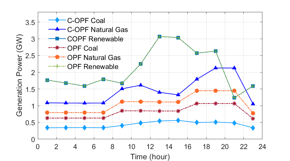
Figure 8: The generation outputs of various power plants over 24 hours under the C-OPF-based and OPF-based economic dispatch schemes.

VI Conclusion

This paper introduces the Carbon-aware Optimal Power Flow (C-OPF) method as a theoretical foundation for decarbonization decision-making in electric power systems. Building upon the OPF approach, C-OPF incorporates generation-side and demand-side carbon emission accounting into power grid decision-making, which enables the optimal management of both energy and carbon emissions. Simulation results demonstrate that C-OPF is an effective tool for carbon-aware power system decision-making that ensures compliance with carbon emissions requirements, especially on the demand side. This paper is a preliminary work that throws some light on the field of the carbon-electricity nexus, and there are still many aspects regarding C-OPF to explore. Three potential future research directions are as follows:

• Theoretical advances in the C-OPF modeling and optimization, such as efficient linearization and convexification of the C-OPF model;

• Adaptation of C-OPF to different settings, such as robust, stochastic, distributed, and online versions;

• Practical applications of C-OPF to power grid decision-making problems, such as carbon-aware grid expansion planning and carbon-electricity pricing.

References

- [1] U.S. Energy Information Administration, “Monthly energy review: May 2023,” 2023.
- [2] World Resources Institute, “GHG protocol scope 2 guidance: An amendment to the GHG protocol corporate standard,” 2015.
- [3] ——, “The greenhouse gas protocol: A corporate accounting and reporting standard,” 2004.
- [4] S. Frank, I. Steponavice, and S. Rebennack, “Optimal power flow: a bibliographic survey i,” Energy systems, vol. 3, no. 3, pp. 221–258, 2012.
- [5] M. B. Cain, R. P. O’neill, A. Castillo et al., “History of optimal power flow and formulations,” Federal Energy Regulatory Commission, vol. 1, pp. 1–36, 2012.
- [6] C. Kang, T. Zhou, Q. Chen, J. Wang, Y. Sun, Q. Xia, and H. Yan, “Carbon emission flow from generation to demand: A network-based model,” IEEE Transactions on Smart Grid, vol. 6, no. 5, pp. 2386–2394, 2015.
- [7] X. Chen, H. Chao, W. Shi, and N. Li, “Towards carbon-free electricity: A comprehensive flow-based framework for power grid carbon accounting and decarbonization,” 2023.
- [8] M. Brander, M. Gillenwater, and F. Ascui, “Creative accounting: A critical perspective on the market-based method for reporting purchased electricity (scope 2) emissions,” Energy Policy, vol. 112, pp. 29–33, 2018.
- [9] A. Bjorn, S. Lloyd, M. Brander, and D. Matthews, “Renewable energy certificates allow companies to overstate their emission reductions,” Nature Climate Change, 2022.
- [10] C. Kang, T. Zhou, Q. Chen, Q. Xu, Q. Xia, and Z. Ji, “Carbon emission flow in networks,” Scientific reports, vol. 2, no. 1, p. 479, 2012.
- [11] Y. Cheng, N. Zhang, Y. Wang, J. Yang, C. Kang, and Q. Xia, “Modeling carbon emission flow in multiple energy systems,” IEEE Transactions on Smart Grid, vol. 10, no. 4, pp. 3562–3574, 2018.
- [12] Y. Sun, C. Kang, Q. Xia, Q. Chen, N. Zhang, and Y. Cheng, “Analysis of transmission expansion planning considering consumption-based carbon emission accounting,” Applied energy, vol. 193, pp. 232–242, 2017.
- [13] W. Shen, J. Qiu, K. Meng, X. Chen, and Z. Y. Dong, “Low-carbon electricity network transition considering retirement of aging coal generators,” IEEE Transactions on Power Systems, vol. 35, no. 6, pp. 4193–4205, 2020.
- [14] Y. Cheng, N. Zhang, and C. Kang, “Bi-level expansion planning of multiple energy systems under carbon emission constraints,” in 2018 IEEE Power & Energy Society General Meeting (PESGM). IEEE, 2018, pp. 1–5.
- [15] T. Wu, X. Wei, X. Zhang, G. Wang, J. Qiu, and S. Xia, “Carbon-oriented expansion planning of integrated electricity-natural gas systems with ev fast-charging stations,” IEEE Transactions on Transportation Electrification, vol. 8, no. 2, pp. 2797–2809, 2022.
- [16] X. Wei, K. W. Chan, T. Wu, G. Wang, X. Zhang, and J. Liu, “Wasserstein distance-based expansion planning for integrated energy system considering hydrogen fuel cell vehicles,” Energy, vol. 272, p. 127011, 2023.
- [17] C. Gu, Y. Liu, J. Wang, Q. Li, and L. Wu, “Carbon-oriented planning of distributed generation and energy storage assets in power distribution network with hydrogen-based microgrids,” IEEE Transactions on Sustainable Energy, 2022.
- [18] Y. Wang, J. Qiu, and Y. Tao, “Optimal power scheduling using data-driven carbon emission flow modelling for carbon intensity control,” IEEE Transactions on Power Systems, vol. 37, no. 4, pp. 2894–2905, 2021.
- [19] L. Sang, Y. Xu, and H. Sun, “Encoding carbon emission flow in energy management: A compact constraint learning approach,” IEEE Transactions on Sustainable Energy, 2023.
- [20] Y. Wang, J. Qiu, and Y. Tao, “Robust energy systems scheduling considering uncertainties and demand side emission impacts,” Energy, vol. 239, p. 122317, 2022.
- [21] Z. Lu, L. Bai, J. Wang, J. Wei, Y. Xiao, and Y. Chen, “Peer-to-peer joint electricity and carbon trading based on carbon-aware distribution locational marginal pricing,” IEEE transactions on power systems, vol. 38, no. 1, pp. 835–852, 2022.
- [22] Washington Department of Commerce, “Energy storage accounting issues,” 2021.
- [23] Federal Energy Regulatory Commission, “Accounting and reporting treatment of certain renewable energy assets,” 2022.
- [24] Y. Gu, J. Li, X. Xing, Z. Cai, G. Deng, T. Sun, and Z. Li, “Carbon emission flow calculation of power systems considering energy storage equipment,” in 2023 8th Asia Conference on Power and Electrical Engineering (ACPEE). IEEE, 2023, pp. 1268–1272.
- [25] P. Shivakumar and K. H. Chew, “A sufficient condition for nonvanishing of determinants,” Proceedings of the American mathematical society, pp. 63–66, 1974.
- [26] T. Ando, “Inequalities for m-matrices,” Linear and Multilinear algebra, vol. 8, no. 4, pp. 291–316, 1980.
- [27] D. Streiffert, “Multi-area economic dispatch with tie line constraints,” IEEE Transactions on Power Systems, vol. 10, no. 4, pp. 1946–1951, 1995.
- [28] B. Hayes, I. Hernando-Gil, A. Collin, G. Harrison, and S. Djokić, “Optimal power flow for maximizing network benefits from demand-side management,” IEEE Transactions on Power Systems, vol. 29, no. 4, pp. 1739–1747, 2014.
- [29] X. Chen, W. Wu, B. Zhang, and C. Lin, “Data-driven dg capacity assessment method for active distribution networks,” IEEE Transactions on Power Systems, vol. 32, no. 5, pp. 3946–3957, 2017.
- [30] G. B. Giannakis, V. Kekatos, N. Gatsis, S.-J. Kim, H. Zhu, and B. F. Wollenberg, “Monitoring and optimization for power grids: A signal processing perspective,” IEEE Signal Processing Magazine, vol. 30, no. 5, pp. 107–128, 2013.
- [31] R. Fletcher* and S. Leyffer, “Solving mathematical programs with complementarity constraints as nonlinear programs,” Optimization Methods and Software, vol. 19, no. 1, pp. 15–40, 2004.
- [32] G. P. McCormick, “Computability of global solutions to factorable nonconvex programs: Part i—convex underestimating problems,” Mathematical programming, vol. 10, no. 1, pp. 147–175, 1976.
- [33] A. Bärmann, R. Burlacu, L. Hager, and T. Kleinert, “On piecewise linear approximations of bilinear terms: structural comparison of univariate and bivariate mixed-integer programming formulations,” Journal of Global Optimization, vol. 85, no. 4, pp. 789–819, 2023.
- [34] P. M. Castro, “Tightening piecewise mccormick relaxations for bilinear problems,” Computers & Chemical Engineering, vol. 72, pp. 300–311, 2015.
- [35] L. T. Biegler and V. M. Zavala, “Large-scale nonlinear programming using ipopt: An integrating framework for enterprise-wide dynamic optimization,” Computers & Chemical Engineering, vol. 33, no. 3, pp. 575–582, 2009.
- [36] X. Chen and N. Li, “Leveraging two-stage adaptive robust optimization for power flexibility aggregation,” IEEE Transactions on Smart Grid, vol. 12, no. 5, pp. 3954–3965, 2021.
- [37] C. Lau and J. Aga, “Bottom line on renewable energy certificates.” 2008.
- [38] Gurobi Optimization, LLC, “Gurobi Optimizer Reference Manual,” 2023. [Online]. Available: https://www.gurobi.com
- [39] X. Chen, “Configuration and parameters of modified 39-bus New England test system,” 2023, [Online]: https://drive.google.com/file/d/1eihAAtEtpxWqY0NvGeX--CVNZZZCDE_B/view?usp=drive_link.