Serverless Federated AUPRC Optimization for Multi-Party Collaborative Imbalanced Data Mining

Abstract.

To address the big data challenges, multi-party collaborative training, such as distributed learning and federated learning, has recently attracted attention. However, traditional multi-party collaborative training algorithms were mainly designed for balanced data mining tasks and are intended to optimize accuracy (e.g., cross-entropy). The data distribution in many real-world applications is skewed and classifiers, which are trained to improve accuracy, perform poorly when applied to imbalanced data tasks since models could be significantly biased toward the primary class. Therefore, the Area Under Precision-Recall Curve (AUPRC) was introduced as an effective metric. Although single-machine AUPRC maximization methods have been designed, multi-party collaborative algorithm has never been studied. The change from the single-machine to the multi-party setting poses critical challenges. For example, existing single-machine-based AUPRC maximization algorithms maintain an inner state for local each data point, thus these methods are not applicable to large-scale online multi-party collaborative training due to the dependence on each local data point.

To address the above challenge, we study serverless multi-party collaborative AUPRC maximization problem since serverless multi-party collaborative training can cut down the communications cost by avoiding the server node bottleneck, and reformulate it as a conditional stochastic optimization problem in a serverless multi-party collaborative learning setting and propose a new ServerLess biAsed sTochastic gradiEnt (SLATE) algorithm to directly optimize the AUPRC. After that, we use the variance reduction technique and propose ServerLess biAsed sTochastic gradiEnt with Momentum-based variance reduction (SLATE-M) algorithm to improve the convergence rate, which matches the best theoretical convergence result reached by the single-machine online method. To the best of our knowledge, this is the first work to solve the multi-party collaborative AUPRC maximization problem. Finally, extensive experiments show the advantages of directly optimizing the AUPRC with distributed learning methods and also verify the efficiency of our new algorithms (i.e., SLATE and SLATE-M).

1. Introduction

Multi-party collaborative learning, such as distributed learning (Dean et al., 2012; Li et al., 2014; Bao et al., 2022) (typically focus on IID data and train learning model using the gradients from different parties) and federated learning (McMahan et al., 2017) (focus on non-IID data and train model via periodically averaging model parameters from different parties coordinated by the server), have been actively studied at past decades to train large-scale deep learning models in a variety of real-world applications, such as computer vision (Goyal et al., 2017; Wu et al., 2022d), natural language processing (Devlin et al., 2018), generative modeling (Brock et al., 2018) and other areas (Li et al., 2023; Ma, 2022; Li et al., 2022; Zhang et al., 2022d). In literature, multi-party collaborative learning is also often called decentralized learning (compared to centralized learning in the single-machine setting). With different network topology, serverless algorithms could be converted into different multi-party collaborative algorithms (seen in 3.1). On the other hand, although there are many ground-breaking studies with DNN in data classification (Goyal et al., 2017; Wei et al., 2021; Wu et al., 2022a; Sun et al., 2022), most works focus on balanced data sets, optimize the cross entropy, and use accuracy to measure model performance. From the viewpoint of optimization, the cross entropy between the estimated probability distribution based on the output of deep learning models and encoding ground-truth labels is a surrogate loss function of the misclassification rate/accuracy. However, in many real-world applications, such as healthcare and biomedicine (Joachims, 2005; Davis and Goadrich, 2006; Zhang et al., 2022a), where patients make up a far smaller percentage of the population than healthy individuals, the data distribution is frequently skewed due to the scarce occurrence of positive samples. The data from the majority class essentially define the result, and the accuracy fails to be an appropriate metric to assess classifiers’ performance. As a result, areas under the curves (AUC), including area under the receiver operating curve (AUROC) and area under precision-recall curves (AUPRC) are given much attention since it excels at discovering models with strong predictive power in imbalanced binary classification (Cortes and Mohri, 2003; Ji et al., 2023).

The prediction performance of models, which are trained with cross entropy as the loss function for imbalanced binary classification, may be subpar because cross-entropy is not the surrogate function of AUC, which call for the study of AUC maximization. Recent works have achieved remarkable progress in directly optimizing AUROC with single-machine and multi-party training algorithms (Zhao et al., 2011; Liu et al., 2019). Liu et al. (2019) constructed deep AUC as a minimax problem and resolved the stochastic AUC maximization problem with a deep neural network as the classifier. Recently, Yuan et al. (2021) and Guo et al. (2020) extended the single-machine training to federated learning and proposed a PL-strongly-concave minimax optimization method to maximize AUROC.

However, AUROC is not suitable for data with a much larger number of negative examples than positive examples, and AUPRC can address this issue because it doesn’t rely on true negatives. Given that an algorithm that maximizes AUROC does not necessarily maximize AUPRC (Davis and Goadrich, 2006) and matching of loss and metric is important (Dou et al., 2022a; Ma et al., 2020; Dou et al., 2022b), the design of AUPRC maximization algorithms has attracted attention (Qi et al., 2021; Wang et al., 2021; Wu et al., 2022b; Jiang et al., 2022; Wang and Yang, 2022). Nonetheless, the multi-party algorithm for AUPRC maximization problems has not been studied. Existing AUPRC optimization methods cannot be directly applied to multi-party collaborative training, since they mainly focus on the finite-sum problem and maintain an inner state for each positive data point, which is not permitted in a multi-party online environment. In addition, to improve communication efficiency, serverless multi-party collaborative learning algorithms are needed to avoid the server node bottleneck in model training. Thus, it is desired to develop efficient stochastic optimization algorithms for serverless multi-party AUPRC maximization for deep learning to meet the challenge of large-scale imbalanced data mining.

The challenges to design serverless multi-party collaborative AUPRC maximization algorithm are three-fold. The first difficulty lies in the complicated integral definition. To overcome the problem of the continuous integral, we can use some point estimators. The average precision (AP) estimator is one of the most popularly used estimators. AP can be directly calculated based on the sample prediction scores and is not subject to sampling bias. It is ideally suited to be used in stochastic optimization problems due to these advantages.

The second difficulty lies in the nested structure and the non-differential ranking functions in the AP. Traditional gradient-based gradient descent techniques cannot directly be used with the original concept of AP. Most existing optimization works use the surrogate function to replace the ranking function in the AP function (Liu et al., 2019; Guo et al., 2020; Qi et al., 2021; Wang et al., 2021; Wu et al., 2022b; Jiang et al., 2022). We can follow these works and substitute a surrogate loss for the ranking function in the AP function.

The third difficulty is that existing algorithms only focus on finite-sum settings and maintain inner estimators $u_{t}$ for each positive data point, which is not permitted in multi-party collaborative online learning. Therefore, despite recent developments, it is still unclear if there is a strategy to optimize AUPRC for multi-party collaborative imbalanced data mining. It is natural to ask the following question: Can we design multi-party stochastic optimization algorithms to directly maximize AUPRC with guaranteed convergence?

In this paper, we provide an affirmative answer to the aforementioned question. We propose the new algorithms for multi-party collaborative AUPRC maximization and provide systematic analysis. Our main contributions can be summarized as follows:

• We cast the AUPRC maximization problem into non-convex conditional stochastic optimization problem by substituting a surrogate loss for the indicator function in the definition of AP. Unlike existing methods that just focus on finite-sum settings, we consider the stochastic online setting.

• We propose the first multi-party collaborative learning algorithm, ServerLess biAsed sTochastic gradiEnt (SLATE), to solve our new objective. It can be used in an online environment and has no reliance on specific local data points. In addition, with different network topologies, our algorithm can also be used for distributed learning and federated learning.

• Furthermore, we propose a stochastic method (i.e., SLATE-M) based on the momentum-based variance-reduced technique to reduce the convergence complexity in multi-party collaborative learning. Our method can reach iteration complexity of $O\left(1/\epsilon^{5}\right)$, which matches the lower bound proposed in the single-machine conditional stochastic optimization.

• Extensive experiments on various datasets compared with baselines verify the effectiveness of our methods.

2. Related work

2.1. AUROC Maximization

There is a long line of research that investigated the imbalanced data mining with AUROC metric (Zhao et al., 2011; Ying et al., 2016; Liu et al., 2019; Yuan et al., 2021; Guo et al., 2020), which highlight the value of the AUC metric in imbalanced data mining. Earlier works about AUROC focused on linear models with pairwise surrogate losses (Joachims, 2005). Furthermore, Ying et al. (2016) solved the AUC square surrogate loss using a stochastic gradient descent ascending approach and provided a minimax reformulation of the loss to address the scaling problem of AUC optimization. Later, Liu et al. (2019) studied the application of AUROC in deep learning and reconstructed deep AUC as a minimax problem, which offers a strategy to resolve the stochastic AUC maximization problem with a deep neural network as the predictive model. Furthermore, some methods were proposed for multi-party AUROC maximization. Yuan et al. (2021) and Guo et al. (2020) reformulated the federated deep AUROC maximization as non-convex-strongly-concave problem in the federated setting. However, the analyses of methods in (Yuan et al., 2021) and (Guo et al., 2020) rely on the assumption of PL condition on the deep models. Recently, (Yuan et al., 2022) developed the compositional deep AUROC maximization model and (Zhang et al., 2023) extend it to federated learning.

2.2. AUPRC Maximization

Early works about AUPRC optimization mainly depend on traditional optimization techniques. Recently, Qi et al. (2021) analyzed AUPRC maximization with deep models in the finite-sum setting. They use a surrogate loss to replace the ranking function in the AP function and maintain biased estimators of the surrogate ranking functions for each positive data point. They proposed the algorithm to directly optimize AUPRC and show a guaranteed convergence. Afterward, Wang et al. (2021) presented adaptive and non-adaptive methods (i.e. ADAP and MOAP) with a new strategy to update the biased estimators for each data point. The momentum average is applied to both the outer and inner estimators to track individual ranking scores. More recently, algorithms proposed in (Wang and Yang, 2022) reduce convergence complexity with the parallel speed-up and Wu et al. (2022b); Jiang et al. (2022) introduced the momentum-based variance-reduction technology into AUPRC maximization to reduce the convergence complexity. While we developed distributed AUPRC optimization concurrently with (Guo et al., 2022), they pay attention to X-Risk Optimization in federated learning. Because X-Risk optimization is a sub-problem in conditional stochastic optimization and federated learning could be regarded as decentralized learning with a specific network topology (seen 3.1), our methods could also be applied to their problem.

Overall, existing methods mainly focus on finite-sum single-machine setting (Qi et al., 2021; Wang et al., 2021; Wu et al., 2022b; Wang and Yang, 2022; Jiang et al., 2022). To solve the biased stochastic gradient, they maintain an inner state for local each data point. However, this strategy limits methods to be applied to real-world big data applications because we cannot store an inner state for each data sample in the online environment. In addition, we cannot extend them directly from the single-machine setting to multi-party setting, because under non-IID assumption, the data point on each machine is different and this inner state can only contain the local data information and make it difficult to train a global model.

In the perspective of theoretical analysis, Hu et al. (2020) studied the general condition stochastic optimization and proposed two single-machine algorithms with and without using the variance-reduction technique (SpiderBoost) named BSGD and BSpiderboost, and established the lower bound at $\varepsilon^{-5}$ in the online setting.

AUPRC is widely utilized in binary classification tasks. It is simple to adapt it for multi-class classifications. If a task has multiple classes, we can assume that each class has a binary classification task and adopt the one vs. the rest classification strategy. We can then calculate average precision based on all classification results.

2.3. Serverless Multi-Party Collaborative Learning

Multi-party collaborative learning (i.e, distributed and federated learning) has wide applications in data mining and machine learning problems (Wang et al., 2023; Zhang et al., 2021c; Mei et al., 2023; Zhang et al., 2022c; Liu et al., 2022a; Luo et al., 2022; He et al., 2023). Multi-party collaborative learning in this paper has a more general definition that does not rely on the IID assumption of data to guarantee the convergence analysis. In the last years, many serverless multi-party collaborative learning approaches have been put out because they avoid the communication bottlenecks or constrained bandwidth between each worker node and the central server, and also provide some level of data privacy (Yuan et al., 2016). Lian et al. (2017) offered the first theoretical backing for serverless multi-party collaborative training. Then serverless multi-party collaborative training attracts attention (Tang et al., 2018; Lu et al., 2019; Liu et al., 2020; Xin et al., 2021) and the convergence rate has been improved using many different strategies, including variance extension (Tang et al., 2018), variance reduction (Pan et al., 2020; Zhang et al., 2021b), gradient tracking (Lu et al., 2019), and many more. In addition, serverless multi-party collaborative learning has been applied to various applications, such as reinforcement learning (Zhang et al., 2021a; He et al., 2020), robust training (Xian et al., 2021), generative adversarial nets (GAN) (Liu et al., 2020), robust principal component analysis (Wu et al., 2023) and other optimization problems (Liu et al., 2022b; Zhang et al., 2022b, 2019, 2020). However, none of them focus on imbalanced data mining. In application, the serverless multi-party collaborative learning setting in this paper is different from federated learning (McMahan et al., 2017) which uses a central server with different communication mechanisms to periodically average the model parameters for indirectly aggregating data from numerous devices. However, with a specific network topology (seen 3.1), federated learning could be regarded as multi-party collaborative learning. Thus, our algorithms could be regarded as a general federated AUPRC maximization.

3. Preliminary

3.1. Serverless Multi-Party Collaborative Learning

Notations: We use $\mathbf{x}$ to denote a collection of all local model parameters $\mathbf{x}_{n}$, where $n\in[N]$, i.e., $\mathbf{x}=[x_{1}^{\top},x_{2}^{\top},\dots,x_{N}^{\top}]^{\top}\in\mathbb{R}^{Nd}$. Similarly, we define $\mathbf{u},\mathbf{v}$ as the concatenation of $\mathbf{u}_{n},\mathbf{v}_{n}$ for $n\in[N]$. In addition, $\otimes$ denotes the Kronecker product, and $\|\cdot\|$ denotes the $\ell_{2}$ norm for vectors, respectively. $\mathcal{D}_{n}^{+}$ denotes the positive dataset on the $N$ worker nodes and $\mathcal{D}$ denotes the whole dataset on the $n$ worker nodes. In multi-party collaborative training, the network system of N worker nodes $\mathcal{G}=(\mathcal{V},\mathcal{E})$ is represented by double stochastic matrix $\underline{\mathbf{W}}=\{\underline{w}_{ij}\}\in\mathbb{R}^{N\times N}$, which is defined as follows: (1) if there exists a link between node i and node j, then $\underline{w}_{ij}>0$, otherwise $\underline{w}_{ij}$ = 0, (2) $\underline{\mathbf{W}}=\underline{\mathbf{W}}^{\top}$ and (3) $\underline{\mathbf{W}}\mathbf{1}=\mathbf{1}$ and $\mathbf{1}^{\top}\underline{\mathbf{W}}=\mathbf{1}^{\top}$. We define the second-largest eigenvalue of $\mathbf{W}$ as $\lambda$ and $\mathbf{W}:=\underline{\mathbf{W}}\otimes\mathbf{I}_{d}$. We denote the exact averaging matrix as $\mathbf{J}=\frac{1}{N}(\mathbf{1}_{n}\mathbf{1}_{n}^{\top})\otimes\mathbf{I}_{d}$ and $\lambda=\|\mathbf{W}-\mathbf{J}\|$. Taking ring network topology as an example, where each node can only exchange information with its two neighbors. The corresponding W is in the form of

(7) $$\small\underline{\mathbf{W}}=\left(\begin{array}[]{cccccc}1/3&1/3&&&&1/3\\ 1/3&1/3&1/3&&&\\ &1/3&1/3&\ddots&&\\ &&\ddots&\ddots&1/3&\\ &&&1/3&1/3&1/3\\ 1/3&&&&1/3&1/3\end{array}\right)\in\mathbb{R}^{N\times N}$$

If we change the network topology, multi-Party collaborative learning could become different types of multi-party collaborative training. If $\mathbf{W}$ is $\frac{1}{N}\mathbf{1}\mathbf{1}^{\top}$, it is converted to distributed learning with the average operation in each iteration. If we choose $\mathbf{W}$ as the Identity matrix and change it to $\frac{1}{N}\mathbf{1}\mathbf{1}^{\top}$ every q iteration, it would be federated learning.

3.2. AUPRC

AUPRC can be defined as the following integral problem (Bamber, 1975):

$$\mathrm{AUPRC}=\int_{-\infty}^{\infty}\operatorname{Pr}(y=1\mid h(\mathbf{x};\mathbf{z})\geq c)d\operatorname{Pr}(h(\mathbf{x};\mathbf{z})\leq c\mid y=1)$$

where $h(\mathbf{x};\mathbf{z})$ is the prediction score function, $\mathbf{x}$ is the model parameter, $\mathbf{\xi}=\left(\mathbf{z},y\right)$ is the data point, and $Pr(y=1|h(\mathbf{x};\mathbf{z})\geq c)$ is the precision at the threshold value of c.

To overcome the problem of the continuous integral, we use AP as the estimator to approximate AUPRC, which is given by (Boyd et al., 2013):

(8) $$\mathrm{AP}=\mathbb{E}_{\mathbf{\xi}\sim\mathcal{D}^{+}}Precision\left(h\left(\mathbf{x};\mathbf{z}\right)\right)=\mathbb{E}_{\mathbf{\xi}\sim\mathcal{D}^{+}}\frac{\mathrm{r}^{+}\left(\mathbf{x};\mathbf{z}\right)}{\mathrm{r}\left(\mathbf{x};\mathbf{z}\right)}$$

where $\mathcal{D}^{+}$ denotes the positive dataset, and samples $\mathbf{\xi}=\left(\mathbf{z},y\right)$ are drawn from positive dataset $\mathcal{D}^{+}$ where $\mathbf{z}\in\mathcal{Z}$ represents the data features and $y=+1$ is the positive label. $\mathrm{r}^{+}$ denotes the positive data rank ratio of prediction score (i.e., the number of positive data points with no less prediction score than that of $\mathbf{\xi}$ including itself over total data number) and $\mathrm{r}$ denotes its prediction score rank ratio among all data points (i.e., the number of data points with no less prediction score than that of $\mathbf{\xi}$ including itself over total data number). $\mathcal{D}$ denotes the whole datasets and $\mathbf{\xi}^{\prime}=(\mathbf{z}^{\prime},y^{\prime})\sim\mathcal{D}$ denote a random data drawn from an unknown distribution $\mathcal{D}$, where $\mathbf{z}^{\prime}\in\mathcal{Z}$ represents the data features and $y^{\prime}\in\mathcal{Y}=\{-1,+1\}$. Therefore, (8) is the same as:

$$\mathrm{AP}=\mathbb{E}_{\mathbf{\xi}\sim\mathcal{D}^{+}}\frac{\mathbb{E}_{\mathbf{\xi}^{\prime}\sim\mathcal{D}}\mathbf{I}(h(\mathbf{x};\mathbf{z}^{\prime})\geq h(\mathbf{x};\mathbf{z}))\cdot\mathbf{I}\left(y^{\prime}=1\right)}{\mathbb{E}_{\mathbf{\xi}^{\prime}\sim\mathcal{D}}\mathbf{I}(h(\mathbf{x};\mathbf{z}^{\prime})\geq h(\mathbf{x};\mathbf{z}))}$$

We employ the following squared hinge loss:

(9) $$\ell\left(\mathbf{x};\mathbf{z},\mathbf{z}^{\prime}\right)=(max\{s-h(\mathbf{x};\mathbf{z})+h(\mathbf{x};\mathbf{z}^{\prime}),0\})^{2}$$

as the surrogate for the indicator function $\mathbf{I}(h(\mathbf{x};\mathbf{z}^{\prime})\geq h(\mathbf{x};\mathbf{z}))$, where $s$ is a margin parameter, that is a common choice used by previous studies (Qi et al., 2021; Wang et al., 2021; Jiang et al., 2022). As a result, the AUPRC maximization problem can be formulated as:

$$AP=\mathbb{E}_{\mathbf{\xi}\sim\mathcal{D}^{+}}\frac{\mathbb{E}_{\mathbf{\xi}^{\prime}\sim\mathcal{D}}\mathbf{I}\left(y^{\prime}=1\right)\ell\left(\mathbf{x};\mathbf{z},\mathbf{z}^{\prime}\right)}{\mathbb{E}_{\mathbf{\xi}^{\prime}\sim\mathcal{D}}\quad\ell\left(\mathbf{x};\mathbf{z},\mathbf{z}^{\prime}\right)}$$

In the finite-sum setting, it is defined as :

$$AP=\frac{1}{|\mathcal{D}^{+}|}\sum_{\mathbf{x}_{i},y_{i}=1}\frac{\mathrm{r}^{+}\left(\mathbf{x}_{i}\right)}{\mathrm{r}\left(\mathbf{x}_{i}\right)}=\frac{1}{|\mathcal{D}^{+}|}\sum_{\mathbf{\xi}\sim\mathcal{D}^{+}}\frac{\frac{1}{|\mathcal{D}|}\sum_{\mathbf{\xi}\sim\mathcal{D}}\mathbf{I}\left(y^{\prime}=1\right)\ell\left(\mathbf{x};\mathbf{z},\mathbf{z}^{\prime}\right)}{\frac{1}{|\mathcal{D}|}\sum_{\mathbf{\xi}\sim\mathcal{D}}\quad\ell\left(\mathbf{x};\mathbf{z},\mathbf{z}^{\prime}\right)}$$

For convenience, we define the elements in $g(\mathbf{x})$ as the surrogates of the two prediction score ranking function $\mathrm{r}^{+}\left(\mathbf{x}\right)$ and $\mathrm{r}\left(\mathbf{x}\right)$ respectively. Define the following equation:

$$g\left(\mathbf{x};\mathbf{\xi},\mathbf{\xi}^{\prime}\right)=\begin{bmatrix}g^{1}\left(\mathbf{x};\mathbf{\xi},\mathbf{\xi}^{\prime}\right)\\ g^{2}\left(\mathbf{x};\mathbf{\xi},\mathbf{\xi}^{\prime}\right)\end{bmatrix}=\begin{bmatrix}\ell\left(\mathbf{x};\mathbf{z},\mathbf{z}^{\prime}\right)\mathbf{I}\left(y^{\prime}=1\right)\\ \ell\left(\mathbf{x};\mathbf{z},\mathbf{z}^{\prime}\right)\end{bmatrix}$$

and $g(\mathbf{x};\mathbf{\xi})=\mathbb{E}_{\mathbf{\xi}^{\prime}\sim\mathcal{D}}g\left(\mathbf{x};\mathbf{\xi},\mathbf{\xi}^{\prime}\right)\in\mathbb{R}^{2}$, and assume $f(\mathbf{u})=-\frac{u_{1}}{u_{2}}:\mathbb{R}^{2}\mapsto\mathbb{R}$ for any $\mathbf{u}=[u_{1},u_{2}]^{\top}\in\mathbb{R}^{2}$. We reformulate the optimization objective into the following stochastic optimization problem:

$$\min_{\mathbf{x}}F(\mathbf{x}) =\mathrm{E}_{\mathbf{\xi}\sim\mathcal{D}^{+}}\left[f(g(\mathbf{x};\mathbf{\xi})\right]$$

(10) $$=\mathrm{E}_{\mathbf{\xi}\sim\mathcal{D}^{+}}\left[f(\mathrm{E}_{\mathbf{\xi}^{\prime}\sim\mathcal{D}}g(\mathbf{x};\mathbf{\xi},\mathbf{\xi}^{\prime}))\right]$$

It is similar to the two-level conditional stochastic optimization (Hu et al., 2020), where the inner layer function depends on the data points sampled from both inner and outer layer functions. Given that $f(\cdot)$ is a nonconvex function, problem (3.2) is a noncvonex optimiztion problem. In this paper, we considers serverless multi-party collaborative non-convex optimization where N worker nodes cooperate to solve the following problem:

(11) $$\min_{\mathbf{x}}F(\mathbf{x}) =\min_{\mathbf{x}}\frac{1}{N}\sum_{n=1}^{n}F_{n}(\mathbf{x})$$

where $F_{n}(\mathbf{x})=\mathbb{E}_{\xi_{n}\sim\mathcal{D}_{n}^{+}}f(\mathbb{E}_{\xi^{\prime}_{n}\sim\mathcal{D}_{n}}g_{n}(\mathbf{x};\xi_{n},\xi^{\prime}_{n}))$ where $\mathbf{\xi}_{n}^{\prime}=(\mathbf{z}_{n}^{\prime},y_{n}^{\prime})\sim\mathcal{D}_{n}$ and $\mathbf{\xi}_{n}=(\mathbf{z}_{n},y_{n})\sim\mathcal{D}^{+}$ We consider heterogeneous data setting in this paper, which refers to a situation where $\mathcal{D}_{i}$ and $\mathcal{D}_{j}$ are different ($i\neq j$ ) on different worker nodes.

In order to design the method, we first consider how to compute the gradient of $F(\mathbf{x})$.

$$\nabla F_{n}(\mathbf{x})= \mathbb{E}_{\xi_{n}\sim\mathcal{D}_{n}^{+}}\nabla g_{n}(\mathbf{x};\xi_{n})^{\top}\nabla f\left(g_{n}(\mathbf{x};\xi_{n})\right)$$

$$= \mathbb{E}_{\xi_{n}\sim\mathcal{D}_{n}^{+}}\nabla g_{n}(\mathbf{x};\xi_{n})^{\top}\left(\frac{-1}{g^{2}_{n}(\mathbf{x};\xi_{n})},\frac{g^{1}_{n}(\mathbf{x};\xi_{n})}{\left(g^{2}_{n}(\mathbf{x};\xi_{n})\right)^{2}}\right)^{\top}$$

where

$$\nabla g_{n}(\mathbf{x};\xi_{n}) =\begin{bmatrix}\nabla g^{1}_{n}(\mathbf{x};\xi_{n})\\ \nabla g^{2}_{n}(\mathbf{x};\xi_{n})\end{bmatrix}$$

$$=\begin{bmatrix}\mathbb{E}_{\xi^{\prime}_{n}\sim\mathcal{D}_{n}}\mathbf{I}\left(y_{n}^{\prime}=1\right)\nabla\ell\left(\mathbf{x};\mathbf{z}_{n},\mathbf{z}_{n}^{\prime}\right)\\ \mathbb{E}_{\xi^{\prime}_{n}\sim\mathcal{D}_{n}}\nabla\ell\left(\mathbf{x};\mathbf{z}_{n},\mathbf{z}_{n}^{\prime}\right)\end{bmatrix}$$

We can notice that it is different from the standard gradient since there are two levels of functions and the inner function also depends on the sample data from the outer layer. Therefore, the stochastic gradient estimator is not an unbiased estimation for the full gradient. Instead of constructing an unbiased stochastic estimator of the gradient (Sun et al., 2023), we consider a biased estimator of $\nabla F_{n}(x)$ using one sample $\xi$ from $\mathcal{D}^{+}_{n}$ and $m$ sample $\xi^{\prime}$ from $\mathcal{D}_{n}$ as $\mathcal{B}_{n}$ in the following form:

(12) $$\nabla\hat{F}_{n}\left(\mathbf{x};\xi_{n},\mathcal{B}_{n}\right)$$

$$= (\frac{1}{m}\sum_{\xi^{\prime}\in\mathcal{B}_{n}}\nabla g_{n}(\mathbf{x};\xi_{n},\xi^{\prime}_{n}))^{\top}\nabla f(\frac{1}{m}\sum_{\xi^{\prime}_{n}\in\mathcal{B}_{n}}g_{n}(\mathbf{x};\xi_{n},\xi^{\prime}_{n}))$$

where $\mathcal{B}_{n}=\left\{\xi^{\prime j}\right\}_{j=1}^{m}$. It is observed that $\nabla\hat{F}_{n}\left(\mathbf{x};\xi_{n},\mathcal{B}_{n}\right)$ is the gradient of an empirical objective such that

$$\hat{F}_{n}\left(\mathbf{x};\xi_{n},\mathcal{B}_{n}\right):=f_{n}\left(\frac{1}{m}\sum_{\xi^{\prime}_{n}\in\mathcal{B}_{n}}g_{n}(\mathbf{x};\xi_{n},\xi^{\prime}_{n})\right)\,.$$

4. Algorithms

In this section, we propose the new serverless multi-party collaborative learning algorithms for solving the problem (11). Specifically, we use the gradient tracking technique ( which could be ignored in practice) and propose a ServerLess biAsed sTochastic gradiEnt (SLATE). We further propose an accelerated version of SLATE with momentum-based variance reduction (Cutkosky and Orabona, 2019) technology (SLATE-M).

4.1. Serverless Biased Stochastic Gradient (SLATE)

Based on the above analysis, we design a serverless multi-party collaborative algorithms with biased stochastic gradient and is named SLATE. Algorithm 1 shows the algorithmic framework of the SLATE. Step 8 could be ignored in practice.

Algorithm 1 SLATE Algorithm

1:  Input: $T$, step size $\eta$ inner batch size $m$ and mini-batch size $b$; $\mathbf{u}_{n,0}=0$ and $\mathbf{v}_{n,0}=0$ for $n\in\{1,\cdots,N\}$

2:  Initialize: $x_{n,0}=\frac{1}{N}\sum_{k=1}^{N}x_{n,0}$.

3:  for $t=0,1,\ldots,T$ do

4:     for $n=1,2,\ldots,N$ do

5:        Draw $b$ samples $\mathcal{B}^{+}_{n,t}=\{\xi^{i}_{n,t}\}_{i=1}^{b}$ from $\mathcal{D}^{+}_{n}$

6:        Draw $m$ samples $\mathcal{B}_{n,t}=\left\{\xi^{\prime j}_{n,t}\right\}_{j=1}^{m}$ from $\mathcal{D}_{n}$,

7:        $\mathbf{u}_{n,t}=\frac{1}{b}\sum_{i=1}^{b}\nabla\hat{F}_{n}(\mathbf{x}_{n,t};\xi^{i}_{n,t},\mathcal{B}_{n,t})$ as in (13)

8:        $\mathbf{v}_{n,t}=\sum_{r=1}^{N}\underline{w}_{nr}(\mathbf{v}_{t-1}^{r}+\mathbf{u}_{t}^{r}-\mathbf{u}_{t-1}^{r})$

9:        $\mathbf{x}_{n,t+1}=\sum_{r=1}^{N}\underline{w}_{nr}(\mathbf{x}_{t}^{n}-\eta\mathbf{v}_{n,t})$

10:     end for

11:  end for

12:  Output: $x$ chosen uniformly random from $\{\bar{\mathbf{x}}_{t}\}_{t=1}^{T}$.

At the beginning of Algorithm 1, one simply initializes local model parameters $\mathbf{x}$ for all worker nodes. Given the couple structure of problem (11). We can assign the value of gradient estimator $\mathbf{u}_{n,0}$ and gradient tracker $\mathbf{v}_{n,0}$ as 0.

At the Lines 5-6 of Algorithm 1, we draw $b$ samples as $\mathcal{B}^{+}_{n,t}$ from positive dataset $\mathcal{D}_{n}^{+}$ and $m$ samples as $\mathcal{B}_{n,t}$from full data sets $\mathcal{D}_{n}$ on each node, respectively. We use a biased stochastic gradient to update the gradient estimator $\mathbf{u}_{n,t}$ according to the (13).

(13) $$\mathbf{u}_{n,t}=$$

$$\sum_{\mathbf{\xi}\in\mathcal{B}^{+}_{n,t}}\sum_{\mathbf{\xi}^{\prime}\in\mathcal{B}_{n,t}}\frac{\left(g^{1}\left(\mathbf{x}_{n,t};\mathbf{\xi},\mathbf{\xi}^{\prime}\right)-g^{2}\left(\mathbf{x}_{n,t};\mathbf{\xi},\mathbf{\xi}^{\prime}\right)\mathbf{I}\left(\mathbf{y}^{\prime}=1\right)\right)\nabla\ell\left(\mathbf{x}_{n,t};\mathbf{z},\mathbf{z}^{\prime}\right)}{bm\left(g^{2}\left(\mathbf{x}_{n,t};\mathbf{\xi},\mathbf{\xi}^{\prime}\right)\right)^{2}}$$

where $\mathbf{\xi}=\left(\mathbf{z},y\right)$ and $\mathbf{\xi}^{\prime}=\left(\mathbf{z}^{\prime},y^{\prime}\right)$

Afterward, at the Line 8 of Algorithm 1 (optional), we adopt the gradient tracking technique (Lu et al., 2019) to reduce network consensus error, where we update the $\mathbf{v}_{n,t}$ and then do the consensus step with double stochastic matrix $\mathbf{W}$ as:

$$\mathbf{v}_{n,t}=\sum_{r=1}^{N}\underline{w}_{nr}(\mathbf{v}_{t-1}^{r}+\mathbf{u}_{t}^{r}-\mathbf{u}_{t-1}^{r})$$

Finally, at the Line 9 of Algorithm 1, we update the model with gradient tracker $\mathbf{v}_{n,t}$, following the consensus step among worker nodes with double stochastic matrix $\mathbf{W}$:

$$\mathbf{x}_{n,t+1}=\sum_{r=1}^{N}\underline{w}_{nr}(\mathbf{x}_{r,t}-\eta\mathbf{v}_{r,t})$$

The output $\bar{\mathbf{x}}_{t}$ is defined as: $\bar{\mathbf{x}}_{t}=\frac{1}{N}\sum_{n=1}^{N}\mathbf{x}_{n,t}\,.$

4.2. SLATE-M

Furthermore, we further propose an accelerated version of SLATE (SLATE-M) based on the momentum-based variance reduced technique, which has the better convergence complexity. The algorithm is shown in Algorithm 2. Step 11 could be ignored in practice.

Algorithm 2 SLATE-M Algorithm

1:  Input: $T$, step size $\eta$, momentum coefficient $\alpha$, inner batch size $m$ and mini-batch size $b$, and initial batch size $B$;

2:  Initialize: $\mathbf{x}_{n,0}=\frac{1}{N}\sum_{k=1}^{N}\mathbf{x}_{n,0}$

3:  Draw $B$ samples of $\{\xi^{i}_{n,0}\}_{i=1}^{B}$ from $\mathcal{D}^{+}_{n}$, and draw $m$ samples $\mathcal{B}_{n,0}=\left\{\xi_{n,0}^{\prime j}\right\}_{j=1}^{m}$ from $\mathcal{D}_{n}$, $\mathbf{u}_{n,0}=\frac{1}{B}\sum_{i=1}^{B}\nabla\hat{F}_{n}(\mathbf{x}_{n,0};\xi^{i}_{n,0},\mathcal{B}_{n,0})\forall n\in[N]$

4:  $\mathbf{v}_{n,0}=\sum_{r=1}^{N}\underline{w}_{nr}\mathbf{u}_{r,0}\forall n\in[N]$

5:  $\mathbf{x}_{n,1}=\sum_{r=1}^{N}\underline{w}_{nr}(\mathbf{x}_{n,0}-\eta\mathbf{v}_{n,0})\forall n\in[N]$

6:  for $t=1,2,\ldots,T$ do

7:     for $n=1,2,\ldots,N$ do

8:        Draw $b$ samples $\mathcal{B}^{+}_{n,t}=\{\xi^{0}_{n,1},\cdots,\xi^{b}_{n,1}\}$ from $\mathcal{D}^{+}_{n}$

9:        Draw $m$ samples $\mathcal{B}_{n,t}=\left\{\xi_{n,t}^{\prime j}\right\}_{j=1}^{m}$ from $\mathcal{D}_{n}$,

10:        $\mathbf{u}_{n,t}=\frac{1}{b}\sum_{i=1}^{b}\nabla\hat{F}_{n}(\mathbf{x}_{n,t};\xi^{i}_{n,t},\mathcal{B}_{n,t})+(1-\alpha)(\mathbf{u}_{n,t-1}-\frac{1}{b}\sum_{i=1}^{b}\nabla\hat{F}_{n}(\mathbf{x}_{n,t-1};\xi^{i}_{n,t},\mathcal{B}_{n,t}))$

11:        $\mathbf{v}_{n,t}=\sum_{r=1}^{N}\underline{w}_{nr}(\mathbf{v}_{t-1}^{r}+\mathbf{u}_{t}^{r}-\mathbf{u}_{t-1}^{r})$

12:        $\mathbf{x}_{n,t+1}=\sum_{r=1}^{N}\underline{w}_{nr}(\mathbf{x}_{t}^{n}-\eta\mathbf{v}_{n,t})$

13:     end for

14:  end for

15:  Output: $x$ chosen uniformly random from $\{\bar{\mathbf{x}}_{t}\}_{t=1}^{T}$.

At the beginning, similar to the SLATE, worker nodes initialize local model parameters $\mathbf{x}$ as seen in Lines 1-2 in Algorithm 2.

Different from SLATE, we initialize the $\mathbf{u}_{n,0}$ with initial batch size $B$ and $\mathbf{v}_{n,0}\forall n\in[N]$, which can be seen in Lines 3-4 in Algorithm 2. Then we do the consensus step to update the model parameters $\mathbf{x}_{n}$. The definition of $\hat{F}_{n}(\mathbf{x}_{n,0};\xi^{i}_{n,0},\mathcal{B}_{n,0})$ is similar to (13) as below:

(14) $$\frac{1}{|\mathcal{B}^{+}_{n,t}|}\hat{F}_{n}(\mathbf{x}_{n,t};\xi^{i}_{n,t},\mathcal{B}_{n,t})=$$

$$\sum_{\mathbf{\xi}\in\mathcal{B}^{+}_{n,t}}\sum_{\mathbf{\xi}^{\prime}\in\mathcal{B}_{n,t}}\frac{\left(g^{1}\left(\mathbf{x}_{n,t};\mathbf{\xi},\mathbf{\xi}^{\prime}\right)-g^{2}\left(\mathbf{x}_{n,t};\mathbf{\xi},\mathbf{\xi}^{\prime}\right)\mathbf{I}\left(\mathbf{y}^{\prime}=1\right)\right)\nabla\ell\left(\mathbf{x}_{n,t};\mathbf{z},\mathbf{z}^{\prime}\right)}{|\mathcal{B}^{+}_{n,t}|m\left(g^{2}\left(\mathbf{x}_{n,t};\mathbf{\xi},\mathbf{\xi}^{\prime}\right)\right)^{2}}$$

where $|\mathcal{B}_{n,t}|$ denotes the size of batch $\mathcal{B}_{n,t}$ and $\mathbf{\xi}=\left(\mathbf{z},y\right)$ and $\mathbf{\xi}^{\prime}=\left(\mathbf{z}^{\prime},y^{\prime}\right)$.

Afterwards, similar to SLATE, each iteration, we draw $b$ samples from positive dataset $\mathcal{D}_{n}^{+}$ and $m$ samples from full data sets $\mathcal{D}_{n}$ on each worker node, respectively to construct the biased stochastic gradient, seen in Line 8-9 of Algorithm 2.

The key different between SLATE and SLATE-M is that we update gradient estimator $\mathbf{u}_{n,t}$ in SLATE-M with the following variance reduction method:

$$\mathbf{u}_{n,t}=\frac{1}{b}\sum_{i=1}^{b}\nabla\hat{F}_{n}(\mathbf{x}_{n,t};\xi^{i}_{n,t},\mathcal{B}_{n,t})+(1-\alpha)(\mathbf{u}_{n,t-1}$$

$$-\frac{1}{b}\sum_{i=1}^{b}\nabla\hat{F}_{n}(\mathbf{x}_{n,t-1};\xi^{i}_{n,t},\mathcal{B}_{n,t}))$$

where $\frac{1}{b}\sum_{i=1}^{b}\nabla\hat{F}_{n}(\mathbf{x}_{n,t};\xi^{i}_{n,t},\mathcal{B}_{n,t})$ and $\frac{1}{b}\sum_{i=1}^{b}\nabla\hat{F}_{n}(\mathbf{x}_{n,t-1};\xi^{i}_{n,t},\mathcal{B}_{n,t})$ are defined in (14)

Finally, we update gradient tracker $\mathbf{v}_{n,t}$ and model parameters $\mathbf{x}_{n,t}$ as in Lines 11-12 in Algorithm 2.

5. Theoretical Analysis

We will discuss some mild assumptions and present the convergence results of our algorithms (SLATE and SLATE-M).

5.1. Assumptions

In this section, we introduce some basic assumptions used for theoretical analysis.

Assumption 1.

$\forall n\in[N]$, we assume (i) there is $C(>0)$ that $\ell(x;z_{n},z_{n})>C$; (ii) there is $M(>0)$ that $0<\ell(x;z_{n},z_{n}^{\prime})<M$; (iii) $\ell(x;z_{n},z_{n}^{\prime})$ is Lipschitz continuous and smooth with respect to model $\mathbf{x}$ for any $\xi_{n}=(z_{n},y_{n})\sim\mathcal{D}^{+},\xi^{\prime}_{n}=(z^{\prime}_{n},y^{\prime}_{n})\sim\mathcal{D}$.

Assumption 2.

$\forall n\in[N]$, we assume there exists a positive constant $\sigma$, such that $\|\nabla g(\mathbf{x};\xi,\xi^{\prime})\|^{2}\leq\sigma^{2},\forall\xi\sim\mathcal{D}_{n}^{+},\xi^{\prime}\sim\mathcal{D}_{n}$

Assumptions 1 and 2 are a widely used assumption in optimization analysis of AUPRC maximization (Qi et al., 2021; Wang et al., 2021; Jiang et al., 2022). They can be easily satisfied when we choose a smooth surrogate loss function $\ell(\mathbf{x};\mathbf{z},\mathbf{z}^{\prime})$ and a bounded score function model $h(\mathbf{x};\cdot)$.

Furthermore, based on Assumptions 1 and 2, we can build the smoothness and lipschitz continuity of objective function in the problem (11).

Lemma 0.

(Lemma 1 in (Wang et al., 2021)) Suppose Assumptions 1 and 2 hold, then $\forall\mathbf{x},\|g_{n}(\mathbf{x};\mathbf{\xi})\|^{2}\leq\sigma_{g}^{2}$, $g_{n}(\mathbf{x};\mathbf{\xi})$ is $L_{g}$-Lipschitz and $S_{g}$-smooth for $\mathbf{xi}\sim\mathcal{D}_{n}^{+}$, and $\forall u\in\Omega,f(u)$ is $L_{f}$-Lipschitz and $S_{f}$-smooth. $\forall\mathbf{x},F_{n}(\mathbf{x})$ is $L_{F}$-Lipschiz and $S_{F}$-smooth.

From the Lemma 1, we have $f_{n}$ and $g_{n}$ are $S_{f}$-smooth and $S_{h}$-smooth. This implies that for an samgle $\mathbf{\xi}_{n}\sim\mathcal{D}_{n}^{+}$ there exist $S_{f}>0$ and $S_{g}>0$ such that

$$\mathbb{E}\|\nabla f_{n}(x_{1})-\nabla f_{n}(x_{2})\|\leq S_{f}\|x_{1}-x_{2}\|$$

$$\mathbb{E}\|\nabla g_{n}(y_{1},\xi_{n})-\nabla g_{n}(y_{2},\xi_{n})\|\leq S_{g}\|y_{1}-y_{2}\|$$

And $f_{n}$ and $g_{n}$ are $L_{f}$-Lipchitz continuous and $L_{g}$-Lipchitz continuous. This implies that there exist $L_{f}>0$ and $L_{g}>0$ such that

$$\mathbb{E}\|\nabla f_{n}(x)\|^{2}\leq L^{2}_{f}$$

$$\mathbb{E}\|\nabla g_{n}(y_{1},\xi_{n})\|^{2}\leq S^{2}_{g}$$

In addition, we also have bounded variance of $g_{n}$. There exist $\sigma_{g}>0$ such that

$$\mathbb{E}_{\xi_{n}\sim\mathcal{D}_{n}^{+}}\|g_{n}(\mathbf{x};\mathbf{\xi}_{n},\mathbf{\xi}^{\prime}_{n})-\mathbb{E}_{\xi_{n}^{\prime}\sim\mathcal{D}_{n}}g_{n}(\mathbf{x};\mathbf{\xi}_{n},\mathbf{\xi}^{\prime}_{n})\|^{2}\leq\sigma_{g}^{2}$$

which indicates that the inner function $g_{n}$ has bounded variance. To control the estimation bias, we follow the analysis in single-machine conditional stochastic optimization (Hu et al., 2020).

Lemma 0.

(Proposition B.1 in (Hu et al., 2020)) Under Assumptions 1 and 2, on the $n$-th worker node, for a sample $\mathbf{\xi}_{n}\sim\mathcal{D}_{n}^{+}$ and $m$ samples $\mathcal{B}_{n}$ from $\mathcal{D}_{n}$,
(a) $\mathcal{B}_{n}=\left\{\xi^{\prime j}\right\}_{j=1}^{m}$ and we have

(15) $$\|\mathbb{E}\nabla\hat{F}_{n}(x;\xi_{n},\mathcal{B}_{n})-\nabla F_{n}(x)\|^{2}\leq\frac{L_{g}^{2}S_{f}^{2}\sigma_{g}^{2}}{m}$$

.
(b) $\mathbb{E}\nabla\hat{F}_{n}(x;\xi_{n},\mathcal{B}_{n})$ are $S_{F}$-Lipschitz smooth
(c)

(16) $$\left\|\nabla\left(f(\hat{g}_{n}(\mathbf{x},\xi_{n}))\right)-\nabla\hat{F}(x)\right\|_{2}^{2}\leq L_{f}^{2}L_{g}^{2}$$

Lemma 2 (a) provide a bound of biased stochastic gradient, which will be used in the following theoretical analysis.

Assumption 3.

The function $F_{n}(x)$ is bounded below, i.e., $\inf_{x}F_{n}(x)>-\infty$.

5.2. The Communication Mechanism in Serverless Multi-Party Collaborative Training

The network system of N worker nodes $\mathcal{G}=(\mathcal{V},\mathcal{E})$ is represented by double stochastic matrix $\underline{\mathbf{W}}=\{\underline{w}_{ij}\}\in\mathbb{R}^{N\times N}$ in the analysis.

For the ease of exposition, we write the $\mathbf{x}_{t}$ and $\mathbf{v}_{t}$-update in Algorithm 1 and Algorithm 2 in the following equivalent matrix form: $\forall t\geq 0$,

$$\mathbf{v}_{t}=\mathbf{W}(\mathbf{v}_{t-1}+\mathbf{u}_{t}-\mathbf{u}_{t-1}),\;\;\mathbf{x}_{t+1}=\mathbf{W}(\mathbf{x}_{t-1}-\eta\mathbf{v}_{t})$$

where $\mathbf{W}:=\underline{\mathbf{W}}\otimes\mathbf{I}_{d}$ and $\mathbf{x}_{t},\mathbf{u}_{t},\mathbf{v}_{t}$ are random vectors in $\mathbb{R}^{Nd}$ that respectively concatenate the local estimates $\{\mathbf{x}_{n,t}\}_{n=1}^{N}$ of a stationary point of $F$ , gradient trackers $\{\mathbf{v}_{n,t}\}_{n=1}^{N}$ , gradient estimators $\{\mathbf{u}_{n,t}\}_{n=1}^{N}$. With the exact averaging matrix $\mathbf{J}$, we have following quantities:

$$\mathbf{1}\otimes\mathbf{\bar{x}}_{t}:=\mathbf{J}\mathbf{x}_{t},\;\mathbf{1}\otimes\bar{\mathbf{u}}_{t}:=\mathbf{J}\mathbf{u}_{t},\;\mathbf{1}\otimes\bar{\mathbf{v}}_{t}:=\mathbf{J}\mathbf{v}_{t}\,$$

Next, we enlist some useful results of gradient tracking-based algorithms for serveress multi-party collaborative stochastic optimization

Lemma 0.

(Lemma 1 in (Xin et al., 2021)) For double stochastic matrix, we have the following:
(a) $\|\mathbf{W}\mathbf{x}-\mathbf{J}\mathbf{x}\|\leq\lambda\|\mathbf{x}-\mathbf{J}\mathbf{x}\|,\forall\mathbf{x}\in\mathbb{R}^{nd}$.
(b) $\bar{\mathbf{v}}_{t}=\bar{\mathbf{u}}_{t},\forall t\geq 0$. As the update step in 1 and 2, we have

$$\bar{\mathbf{x}}_{t+1}=\bar{\mathbf{x}}_{t}-\eta\bar{\mathbf{v}}_{t}=\bar{\mathbf{x}}_{t}-\eta\bar{\mathbf{u}}_{t}$$

(c) According to the definition of network $\mathbf{W}$, we have the following inequalities: $\forall k\geq 0$,

(17) $$\left\|\mathbf{x}_{t+1}-\mathbf{J}\mathbf{x}_{t+1}\right\|^{2}\leq\frac{1+\lambda^{2}}{2}\left\|\mathbf{x}_{t}-\mathbf{J}\mathbf{x}_{t}\right\|^{2}+\frac{2\eta^{2}\lambda^{2}}{1-\lambda^{2}}\left\|\mathbf{v}_{t}-\mathbf{Jv}_{t}\right\|^{2}$$

(18) $$\left\|\mathbf{x}_{t+1}-\mathbf{J}\mathbf{x}_{t+1}\right\|^{2}\leq 2\lambda^{2}\left\|\mathbf{x}_{t}-\mathbf{J}\mathbf{x}_{t}\right\|^{2}+2\eta^{2}\lambda^{2}\left\|\mathbf{v}_{t}-\mathbf{J}\mathbf{v}_{t}\right\|^{2}$$

(19) $$\left\|\mathbf{x}_{t+1}-\mathbf{J}\mathbf{x}_{t+1}\right\|\leq\lambda\left\|\mathbf{x}_{t}-\mathbf{J}\mathbf{x}_{t}\right\|^{2}+\eta\lambda\left\|\mathbf{v}_{t}-\mathbf{J}\mathbf{v}_{t}\right\|$$

Then, we study the convergence properties of SLATE and SLATEM. We first discus the metric to measure convergence of our algorithms. Given that the loss function is nonconvex, we are unable to demonstrate convergence to an global minimum point. Instead, we establish convergence to an approximate stationary point, defined below:

Definition 0.

A point $x$ is called $\epsilon$-stationary point if $\|\nabla f(x)\|\leq\epsilon$. Generally, a stochastic algorithm is defined to achieve an $\epsilon$-stationary point in $T$ iterations if $\mathbb{E}\|\nabla f(x_{T})\|\leq\epsilon$.

5.3. Convergence Analysis of SLATE Algorithm

First, we study the convergence properties of our SLATE algorithm. The detailed proofs are provided in the supplementary materials.

Theorem 5.

Suppose the sequence $\{\mathbf{\bar{x}}_{t}\}_{t=1}^{T}$ be generated from Algorithm 1 and Assumptions 1, 2, and 3 hold, $0<\eta\leq\min\{\frac{1-\lambda^{2}}{24\lambda^{2}S_{F}},\frac{1}{6S_{F}}\}$, SLATE in algorithm 1 has the following

$$\frac{1}{T}\sum_{t=0}^{T-1}\mathbb{E}\|\nabla F(\bar{\mathbf{x}}_{t})\|^{2}\leq\frac{2\mathbb{E}[F(\bar{\mathbf{x}}_{0})-F(\bar{\mathbf{x}}_{T})]}{\eta T}$$

$$+\left(\frac{1}{\lambda^{2}}+5N\right)\frac{32\lambda^{2}\eta^{2}L_{f}^{2}L_{g}^{2}S_{F}^{2}}{(1-\lambda^{2})^{2}N}+\frac{2L_{g}^{2}S_{f}^{2}\sigma_{g}^{2}}{m}+\frac{2\eta S_{F}L_{f}^{2}L_{g}^{2}}{N}$$

Corollary 0.

Based on the analysis in Theorem 5, by setting $\eta=O(\sqrt{\frac{N}{T}})$ , SLATE in Algorithm 1 has the following

$$\frac{1}{T}\sum_{t=0}^{T-1}\mathbb{E}\|\nabla F(\bar{\mathbf{x}}_{t})\|^{2}\leq O(\frac{\mathbb{E}[F(\bar{\mathbf{x}}_{0})-F(\bar{\mathbf{x}}_{T})]}{(NT)^{1/2}})$$

$$+\left(\frac{1}{\lambda^{2}}+5\right)\frac{24\lambda^{2}L_{f}^{2}L_{g}^{2}S_{F}^{2}}{(1-\lambda^{2})^{2}}O(\frac{N}{T})+\frac{2L_{g}^{2}S_{f}^{2}\sigma_{g}^{2}}{m}+O(\frac{2S_{F}L_{f}^{2}L_{g}^{2}}{(NT)^{1/2}})$$

Based on the result in Theorem 5 and Corollary 6, we can get the convergence result of SLATE.

Remark 1.

According to Corollary 6, without loss of generality, we let $m=O(\varepsilon^{-2})$, $b=O(1)$ and $\sqrt{T}>N$, we know to make $\frac{1}{T}\sum_{t=0}^{T-1}\mathbb{E}\|\nabla F(\bar{\mathbf{x}}_{t})\|^{2}\leq\varepsilon^{2}$, we have iterations $T$ should be as large as $O(N^{-1}\varepsilon^{-4})$.

In Algorithm 1, we sample $b+m$ data points to build the biased stochastic gradients $\mathbf{u}_{n,t}$, and need $T$ iterations. Thus, our SLATE algorithm has a sample complexity of $m\cdot T=O(N^{-1}\varepsilon^{-6})$, for finding an $\epsilon$-stationary point. In addition, the result also indicates the linear speedup of our algorithm with respect to the number of worker nodes.

5.4. Convergence Analysis of SLATE-M

In the subsection, we study the convergence properties of our SLATE-M algorithm. The details about proofs are provided in the supplementary materials.

Theorem 7.

Suppose the sequence $\{\mathbf{\bar{x}}_{t}\}_{t=1}^{T}$ be generated from Algorithm 2 and Assumptions 1, 2, and 3 hold, $0<\eta\leq min\{\frac{1}{4},\\ \frac{\left(1-\lambda^{2}\right)^{2}}{90\lambda^{2}},\frac{\sqrt{1-\lambda^{2}}}{12\sqrt{7}\lambda}\}\frac{1}{S_{F}}$ and $\alpha=\frac{72S^{2}_{F}\eta^{2}}{Nb}$ , SLATE-M in Algorithm 2 has the following

$$\frac{1}{T}\sum_{t=0}^{T-1}\mathbb{E}\|\nabla\mathbf{F}(\bar{\mathbf{x}}_{t})\|^{2}\leq\frac{2(\mathbf{F}(\bar{\mathbf{x}}_{0})-\mathbf{F}(\bar{\mathbf{x}}_{T}))}{\eta T}+\frac{3L_{g}^{2}S_{f}^{2}\sigma_{g}^{2}}{m}+3\frac{L_{g}^{2}L_{f}^{2}}{\alpha NBT}$$

$$+\frac{6\alpha L_{g}^{2}L_{f}^{2}}{Nb}+\frac{96\lambda^{2}L_{g}^{2}L_{f}^{2}}{\left(1-\lambda^{2}\right)^{3}BT}+\frac{256\lambda^{2}\alpha^{2}L_{f}^{2}L_{g}^{2}}{(1-\lambda^{2})^{3}}+\frac{64\lambda^{4}\mathbb{E}\left\|\nabla\hat{\mathbf{F}}_{0}\right\|^{2}}{(1-\lambda^{2})^{3}NT}$$

Corollary 0.

Based on the analysis in the theorem 7, we choose $b=O(1),\eta=O(\frac{N^{2/3}}{T^{1/3}}),\alpha=O(\frac{N^{1/3}}{T^{2/3}}),B=O(\frac{T^{1/3}}{N^{2/3}})$, SLATE-M in Algorithm 2 has the following

$$\frac{1}{T}\sum_{t=0}^{T-1}\mathbb{E}\|\nabla\mathbf{F}(\bar{\mathbf{x}}_{t})\|^{2}\leq O(\frac{2(\mathbf{F}(\bar{\mathbf{x}}_{0})-\mathbf{F}(\bar{\mathbf{x}}_{T}))}{(NT)^{2/3}}+\frac{3L_{g}^{2}S_{f}^{2}\sigma_{g}^{2}}{m}$$

$$+O(\frac{3L_{g}^{2}L_{f}^{2}}{(NT)^{2/3}})+O(\frac{6L_{g}^{2}L_{f}^{2}}{(NT)^{2/3}})+\frac{352\lambda^{2}L_{f}^{2}L_{g}^{2}}{(1-\lambda^{2})^{3}}O(\frac{N^{2/3}}{T^{4/3}})$$

(20) $$+\frac{64\lambda^{4}\mathbb{E}\left\|\nabla\hat{\mathbf{F}}_{0}\right\|^{2}}{(1-\lambda^{2})^{3}NT}$$

Based on the result in theorem 7, we can get the convergence result of SLATE-M.

Remark 2.

According to Corollary 8, without loss of generality, Let $m=O(\varepsilon^{-2})$, $b=O(1)$ $\eta=O(\frac{N^{2/3}}{T^{1/3}}),\alpha=O(\frac{N^{1/3}}{T^{2/3}})$, and $B=O(\frac{T^{1/3}}{N^{2/3}})$, we know to make $\frac{1}{T}\sum_{t=0}^{T-1}\mathbb{E}\|\nabla F(\bar{\mathbf{x}}_{t})\|^{2}\leq\varepsilon^{2}$, we have iterations $T$ should be as large as $O(N^{-1}\varepsilon^{-3})$.

In Algorithm 2, in each iteration, we sample $b+m$ data points to build the biased stochastic gradients $\mathbf{u}_{n,t}$, and need $T$ iterations. Thus, our SLATE-M algorithm has a sample complexity of $m\cdot T=O(N^{-1}\varepsilon^{-5})$, for finding an $\epsilon$-stationary point, which also achieves the linear speedup of our algorithm with respect to the number of worker nodes.

Remark 3.

The sample complexity of $O(N^{-1}\varepsilon^{-5})$ in SLATE-M matches the best convergence complexity achieved by the single-machine stochastic method for conditional stochastic optimization in the online setting, and also match the lower bound for the online stochastic algorithms (Hu et al., 2020).

6. Experiments

In this section, we conduct extensive experiments on imbalanced benchmark datasets to show the efficiency of our algorithms. All experiments are run over a machine with AMD EPYC 7513 32-Core Processors and NVIDIA RTX A6000 GPU. The source code is available at https://github.com/xidongwu/D-AUPRC.

The goal of our experiments is two-fold: (1) to verify that (11) is the surrogate function of AUPRC and illustrate that directly optimizing the AUPRC in the multi-party collaborative training would improve the model performance compared with traditional loss optimization, and (2) to show the efficiency of our methods for AUPRC maximization.

Table 1. Statistics of benchmark datasets

Data Set	Training examples	Testing examples	Feature Size	Proportion of positive data
w7a	24692	25057	300	2.99%
w8a	49749	14951	300	2.97 %
MNIST	60000	10000	$28\times 28$	16.7%
Fashion MNIST	60000	10000	$28\times 28$	16.7 %
CIFAR-10	50000	10000	$3\times 32\times 32$	16.7 %
Tiny-ImageNet	100000	10000	$3\times 64\times 64$	16.7 %

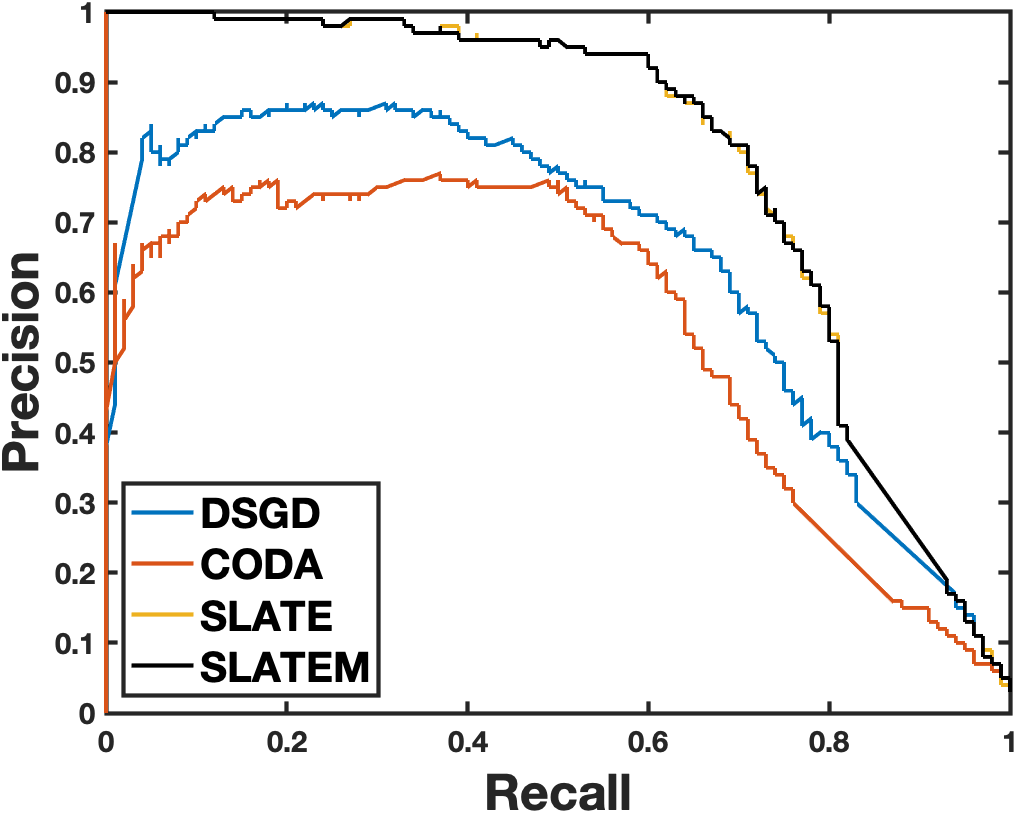
(a) w7a dataset

(b) MNIST dataset

(c) CIFAR-10 dataset

Figure 1. Precision-Recall curves of the models on the testing set

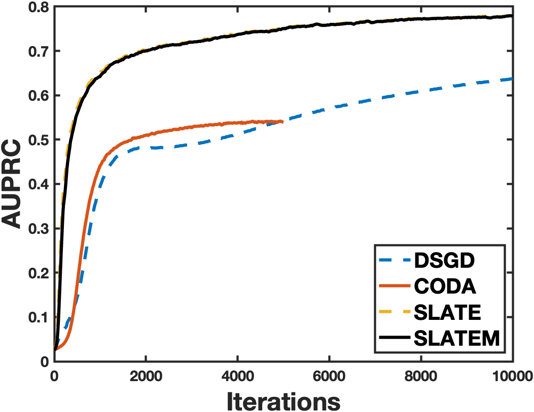
(a) w7a dataset

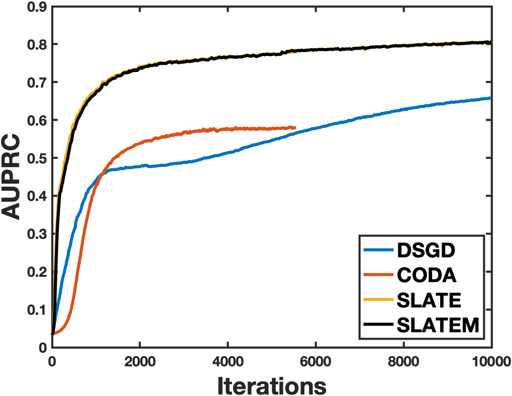
(b) w8a dataset

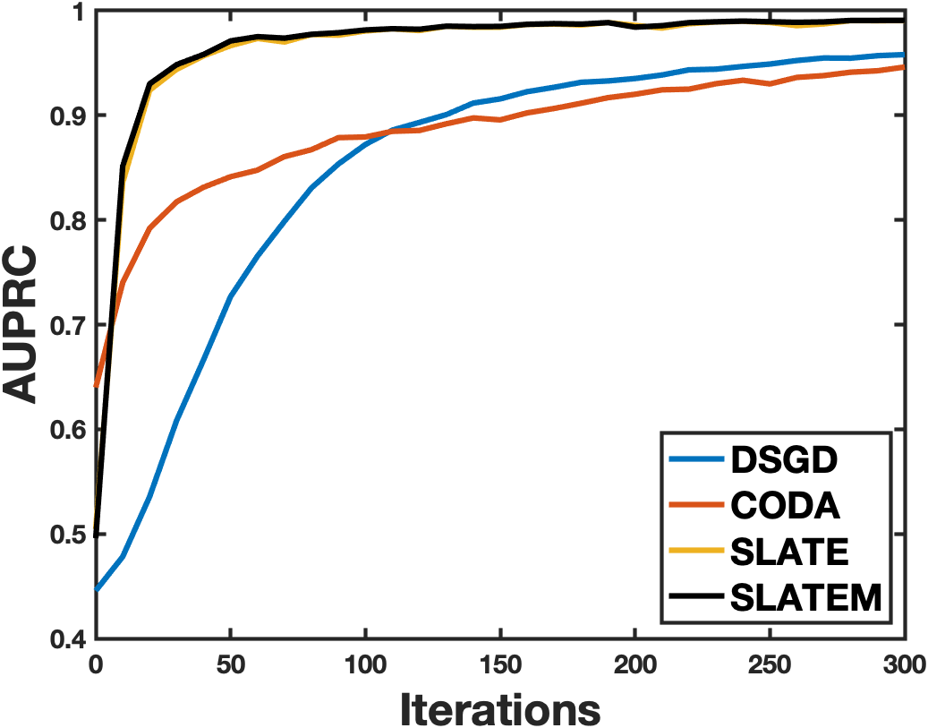
(c) MNIST dataset

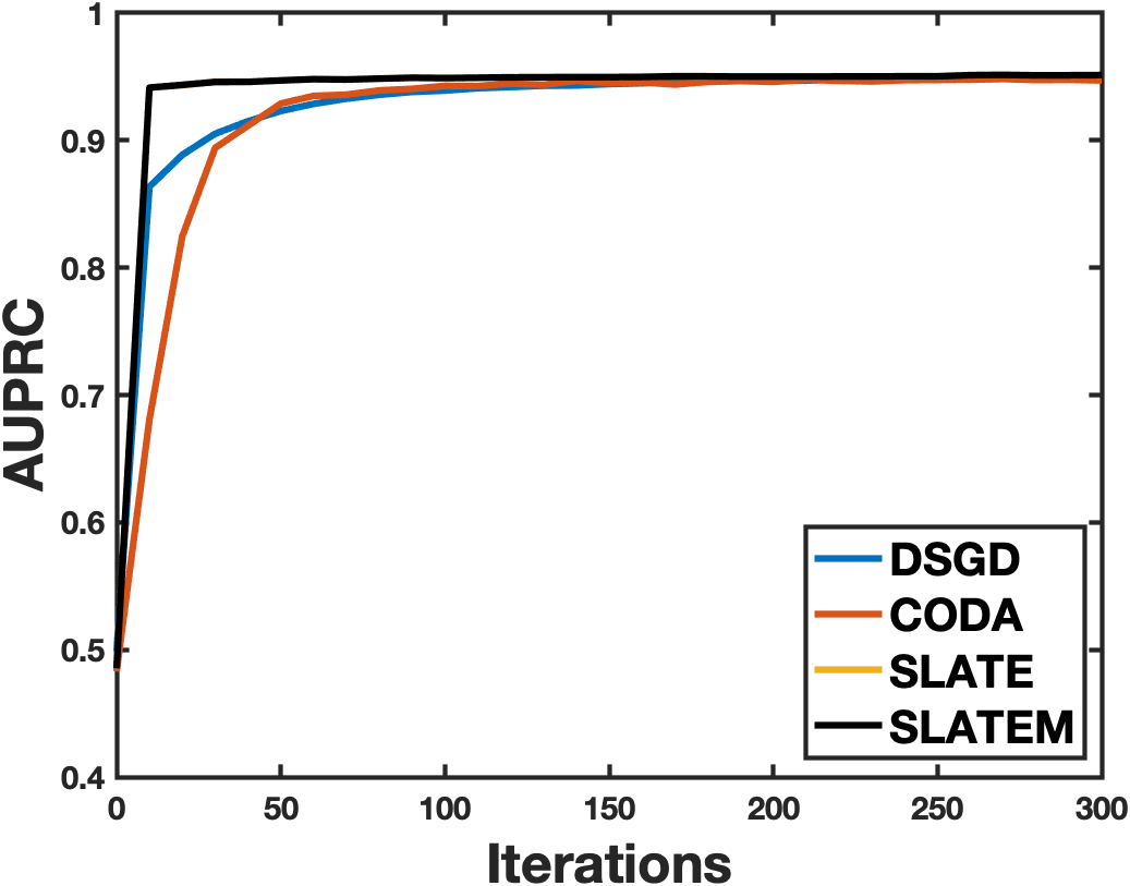
(d) Fashion MNIST dataset

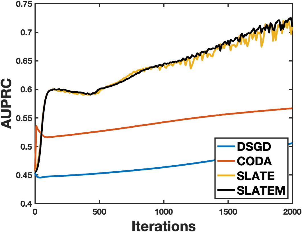
(e) CIFAR-10 dataset

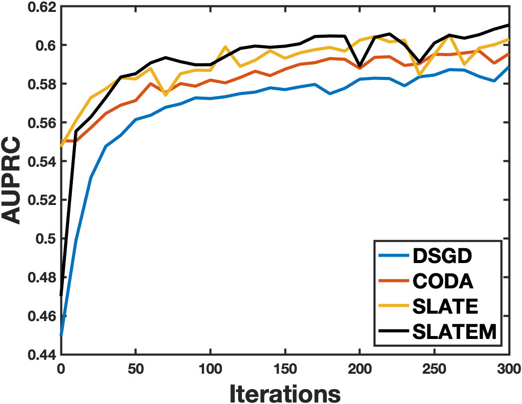
(f) Tiny-ImageNet dataset

Figure 2. AP vs Iterations on the test set

Table 2. Final averaged AP scores on the testing data

Method	w7a	w8a	MNIST	Fashion MNIST	CIFAR-10	Tiny-ImageNet
D-PSGD	0.6372	0.6585	0.9592	0.9497	0.5058	0.5906
CODA	0.5414	0.5786	0.9460	0.9474	0.5668	0.5971
SLATE	0.7788	0.8072	0.9911	0.9515	0.7279	0.6032
SLATEM	0.7778	0.8063	0.9913	0.9515	0.7285	0.6131

6.1. Configurations

Datasets: We conduct experiments on imbalanced benchmark datasets from LIBSVM data : w7a and w8a, and four typical image datasets: MNIST dataset, Fashion-MNIST dataset, CIFAR-10, and Tiny-ImageNet dataset (seen in Table 1). For w7a and w8a, we scale features to [0, 1]. For image datasets, following (Qi et al., 2021; Wang et al., 2021), we construct the imbalanced binary-class versions as follows: Firstly, the first half of the classes (0 - 4) in the original MNIST, Fashion-MNIST, and CIFAR-10, and (0 - 99) in Tiny-ImageNet datasets are converted to be the negative class, and another half of classes are considered to be the positive class. Because the original distributions of image datasets are balanced, we randomly drop 80% of the positive examples in the training set to make them imbalanced and keep test sets of image datasets unchanged. Finally, we evenly partition each datasets into disjoint sets and distribute datasets among worker nodes.

Models: For w7a and w8a, we use two layers of neural networks with the dimension of the hidden layer as 28. The RELU is used as the activation function. For MNIST, Fashion MNIST and Cifar-10 data sets, we choose model architectures from (Wu et al., 2022c) for our imbalanced binary image classification task. For Tiny-ImageNet, we choose ResNet-18 (He et al., 2016) as the classifier. In our algorithms, We modify the output of all models to 1 and the sigmoid function is followed since we consider binary classification tasks.

In the experiments, the number of worker nodes is set as N = 20 and we use the ring-based topology as the communication network structure. (Lian et al., 2017).

6.2. Comparison with Existing Multi-Party Stochastic Methods

Baselines: We compare our algorithms with two baselines: 1) D-PSGD (Lian et al., 2017), a SGD-like serverless multi-party collaborative algorithm with the Cross-Entropy loss as the optimization objective. D-PSGD runs SGD locally and then computes the neighborhood weighted average by fetching model parameters from neighbors; 2) CODA, a typical federated learning algorithm for optimizing minimax formulated AUROC loss (Guo et al., 2020; Yuan et al., 2021). CODA runs local SGDA with the periodic model average in the federated learning setting. We convert it into the serverless multi-party setting and run local SGDA, following the consensus step to update the models. Gradient tracking steps are ignored. In the experiments, we ignore the gradient tracking steps to reduce computation and communication costs.

Parameter tuning: We perform a grid search to tune all methods carefully. The total batch size m drawn from $\mathcal{D}$ is chosen in the set $\{20,20,20,20,60,200\}$. For SLATE and SLATE-M, the positive batch size b in the total batch size is chosen in the set $\{2,2,3,5,20,35\}$, and m - b negative data points. The squared hinge loss is used as (9), $\alpha$ is chosen from $\{0.1,0.9\}$ and the margin parameter s is selected from $\{0.1,0.3,0.5,0.7,0.9\}$. The step size is selected from the set $\{0.01,0.005,0.001\}$. For the D-PSGD, the step size is chosen in the set $\{0.01,0.005,0.001\}$. For the CODA, the step size for minimum variable is chose from the set $\{0.01,0.005,0.001\}$ and that for the maximum variable is chosen from the set $\{0.0001,0.0005,0.001\}$. Moreover, we use Xavier normal to initialize models.

Table 3. SLATE test accuracy on CIFAR-10 with margin parameter $s$, and positive batch size b (B=60)

Margin	0.1	0.3	0.5	0.7	0.9
b = 5	0.6270	0.5971	0.5992	0.5928	0.5765
b = 10	0.6910	0.5887	0.5956	0.5986	0.5989
b = 15	0.7248	0.5895	0.5902	0.5952	0.5979
b = 20	0.7279	0.6001	0.5870	0.5929	0.5962
b = 25	0.7216	0.6038	0.5876	0.5933	0.5962

Table 4. SLATE-M test accuracy on CIFAR-10 with margin parameter $s$, positive batch size b (B = 60), and $\alpha$

Margin	0.1 ($\alpha$ = 0.1)	0.1 ($\alpha$ = 0.9)	0.3 ($\alpha$ = 0.1)	0.3 ($\alpha$ = 0.9)
b = 15	0.7273	0.7272	0.5853	0.5895
b = 20	0.7285	0.7289	0.5986	0.6001
b = 25	0.7167	0.7206	0.6024	0.6036

Experimental results: Table 2 summarizes the final results on the test sets. In order to present the advantage of optimization of AUPRC, we plot the Precision-Recall curves of final models on testing sets of W7A, MNIST, and CIFAR-10 when training stop in Figure 1. Then we illustrate the convergence curve on test sets in Figure 2. Results show that our algorithms (i.e., SLATE, SLATE-M) can outperform baselines in terms of AP with a great margin across each benchmark, regardless of model structure. The experiments verify that 1) the objective function (11) is a good surrogate loss function of AUPRC and directly optimizing the AUPRC in the multi-party collaborative training would improve the model performance compared with traditional loss optimization in the imbalanced data mining. 2) Although CODA, with minimax formulated AUROC loss, has a relatively better performance compared with D-PSGD in large-scale datasets (CIFAR-10 and Tiny-ImageNet), the results verify the previous results that an algorithm that maximizes AUROC does not necessarily maximize AUPRC. Therefore, designing the algorithms for AUPRC in multi-party collaborative training is necessary. 3) our algorithms can efficiently optimize the (11) and largely improve the performance in terms of AUPRC in multi-party collaborative imbalanced data mining. 4) In datasets CIFAR-10 and Tiny-ImageNet, SLATE-M has better performance compared with SLATE.

Ablation study: In this part, we study the effect of margin parameters, positive batch size, and $\alpha$ of SLATE-M. The results are listed in Table 3 and Table 4.

7. Conclusion

In this paper, we systematically studied how to design serverless multi-party collaborative learning algorithms to directly maximize AUPRC and also provided the theoretical guarantee on algorithm convergence. To the best of our knowledge, this is the first work to optimize AUPRC in the multi-party collaborative training. We cast the AUPRC maximization problem into non-convex two-level stochastic optimization functions under the multi-party collaborative learning settings as the problem (11), and proposed the first multi-party collaborative learning algorithm, ServerLess biAsed sTochastic gradiEnt (SLATE). Theoretical analysis shows that SLATE has a sample complexity of $O(\varepsilon^{-6})$ and shows a linear speedup respective to the number of worker nodes. Furthermore, we proposed a stochastic method (i.e., SLATE-M) based on the momentum-based variance-reduced technique to reduce the convergence complexity for maximizing AP in multi-party collaborative optimization. Our methods reach iteration complexity of $O\left(1/\epsilon^{5}\right)$, which matches the best convergence complexity achieved by the single-machine stochastic method for conditional stochastic optimization in the online setting, and also matches the lower bound for the online stochastic algorithms. Unlike existing single-machine methods that just focus on finite-sum settings and must keep an inner state for each positive data point, we consider the stochastic online setting. The extensive experiments on various data sets compared with previous stochastic multi-party collaborative optimization algorithms validate the effectiveness of our methods. Experimental results also demonstrate that directly optimizing the AUPRC in the multi-party collaborative training would largely improve the model performance compared with traditional loss optimization.

Appendix A Supplementary material

A.1. Basic Lemma

We draw one sample $\xi_{n}$ from $\mathcal{D}^{+}_{n}$ and $m$ sample $\xi^{\prime}_{n}$ from $\mathcal{D}_{n}$ as $\mathcal{B}_{n}$. We define

$$g_{n}(x;\mathbf{\xi}_{n})=\mathbb{E}_{\mathbf{\xi}_{n}^{\prime}\sim\mathcal{D}_{n}}g_{n}\left(x;\mathbf{\xi}_{n},\mathbf{\xi}_{n}^{\prime}\right)$$

$$\hat{g}_{n}(x,\xi_{n})=\frac{1}{m}\sum_{\xi_{n}^{\prime}\in\mathcal{B}_{n}}g_{n}(x,\xi_{n};\xi_{n}^{\prime})$$

$$\hat{F}_{n}(x;\xi_{n},\mathcal{B}_{n})=f(\hat{g}_{n}(x,\xi_{n}))$$

We also define

$$\nabla F_{n}(x)=\nabla\mathbb{E}_{\xi_{n}}f(g_{n}(x,\xi_{n}))=\mathbb{E}_{\xi_{n}}\left[\nabla\left(f(g_{n}(x,\xi_{n}))\right)\right]=\mathbb{E}_{\xi_{n}}\left[\nabla f(g_{n}(x,\xi_{n}))\cdot\nabla g_{n}(x,\xi_{n})\right]$$

$$\hat{F}_{n}(x)=\mathbb{E}\hat{F}_{n}(x;\xi_{n},\mathcal{B}_{n})=\mathbb{E}\left[f(\hat{g}_{n}(x,\xi_{n}))\right]$$

(21) $$\nabla\hat{F}_{n}(x)=\mathbb{E}\nabla\hat{F}_{n}(x;\xi_{n},\mathcal{B}_{n})$$

For convenience, we denote

(22) $$\bar{\mathbf{x}}_{t}=\frac{1}{N}\sum_{n=1}^{N}\mathbf{x}_{n,t},\quad\bar{\mathbf{v}}_{t}=\frac{1}{N}\sum_{n=1}^{N}\mathbf{v}_{n,t},\quad\bar{\mathbf{u}}_{t}=\frac{1}{N}\sum_{n=1}^{N}\mathbf{u}_{n,t}\quad F(\bar{\mathbf{x}})=\frac{1}{N}\sum_{n=1}^{N}F_{n}(\bar{\mathbf{x}}),\nabla\hat{F}(\bar{\mathbf{x}})=\frac{1}{N}\sum_{n=1}^{N}\nabla\hat{F}_{n}(\bar{\mathbf{x}})$$

and $\nabla\hat{\mathbf{F}}_{t}=[\nabla\hat{F}_{1}(\mathbf{x}_{1})^{\top},\nabla\hat{F}_{2}(\mathbf{x}_{2})^{\top},\dots,\nabla\hat{F}_{N}(\mathbf{x}_{N})^{\top}]^{\top}\in\mathbb{R}^{nd}$.

Lemma 0.

(Lemma 6 in (Xin et al., 2021)) Let $\{V_{t}\}_{t\geq 0},\{R_{t}\}_{t\geq 0}$ and $\{Q_{t}\}_{t\geq 0}$ be non-negative sequences and $C\geq 0$ be some constant such that $V_{t}\leq qV_{t-1}+qR_{t-1}+Q_{t}+C,\forall t\geq 1$, where $q\in(0,1)$ Then the following inequality holds: $\forall T\geq 1$,

(23) $$\sum_{t=0}^{T-1}V_{t}\leq\frac{V_{0}}{1-q}+\frac{1}{1-q}\sum_{t=0}^{T-2}R_{t}+\frac{1}{1-q}\sum_{t=1}^{T-1}Q_{t}+\frac{CT}{1-q}$$

Appendix B SLATE

B.1. Proofs of the Intermediate Lemmas

Lemma 0.

Let Assumptions 1, 2 hold, and $F$ is $S_{F}$-smooth, we have

$$\mathbb{E}F(\bar{\mathbf{x}}_{t+1}) \leq\mathbb{E}F(\bar{\mathbf{x}}_{t})-(\frac{\eta}{2}-\eta^{2}S_{F})\mathbb{E}\|\nabla\hat{F}(\bar{\mathbf{x}}_{t})\|^{2}-\frac{\eta}{2}\mathbb{E}\|\nabla F(\bar{\mathbf{x}}_{t})\|^{2}$$

(24) $$+\frac{\eta S_{F}^{2}}{N}\sum_{n=1}^{N}\|x_{n,t}-\bar{\mathbf{x}}_{t}\|^{2}+\frac{\eta L_{g}^{2}S_{f}^{2}\sigma_{g}^{2}}{m}+\frac{\eta^{2}S_{F}L_{f}^{2}L_{g}^{2}}{N}$$

Proof.

Based on the smoothness of F, we have

$$\mathbb{E}F(\bar{\mathbf{x}}_{t+1}) \stackrel{{\scriptstyle(a)}}{{\leq}}\mathbb{E}F(\bar{\mathbf{x}}_{t})+\mathbb{E}\langle\nabla F(\bar{\mathbf{x}}_{t}),\bar{\mathbf{x}}_{t+1}-\bar{\mathbf{x}}_{t}\rangle+\frac{S_{F}}{2}\mathbb{E}\left\|\bar{\mathbf{x}}_{t+1}-\bar{\mathbf{x}}_{t}\right\|^{2}$$

$$\stackrel{{\scriptstyle(b)}}{{\leq}}\mathbb{E}F(\bar{\mathbf{x}}_{t})-\eta\mathbb{E}\langle\nabla F(\bar{\mathbf{x}}_{t}),\bar{\mathbf{u}}_{t}\rangle+\frac{\eta^{2}S_{F}}{2}\mathbb{E}\|\bar{\mathbf{u}}_{t}\|^{2}$$

$$\stackrel{{\scriptstyle(c)}}{{\leq}}\mathbb{E}F(\bar{\mathbf{x}}_{t})-\eta\mathbb{E}\langle\nabla F(\bar{\mathbf{x}}_{t}),\frac{1}{N}\sum_{n=1}^{N}\nabla\hat{F}_{n}(\mathbf{x}_{n,t})\rangle+\eta^{2}S_{F}\mathbb{E}[\|\bar{\mathbf{u}}_{t}-\frac{1}{N}\sum_{n=1}^{N}\nabla\hat{F}_{n}(\mathbf{x}_{n,t})\|^{2}+\|\frac{1}{N}\sum_{n=1}^{N}\nabla\hat{F}_{n}(\mathbf{x}_{n,t})\|^{2}]$$

$$\stackrel{{\scriptstyle(d)}}{{=}}\mathbb{E}F(\bar{\mathbf{x}}_{t})-(\frac{\eta}{2}-\eta^{2}S_{F})\mathbb{E}\|\frac{1}{N}\sum_{n=1}^{N}\nabla\hat{F}_{n}(\mathbf{x}_{n,t})\|^{2}-\frac{\eta}{2}\mathbb{E}\|\nabla F(\bar{\mathbf{x}}_{t})\|^{2}+\frac{\eta}{2}\mathbb{E}\|\nabla F(\bar{\mathbf{x}}_{t})-\frac{1}{N}\sum_{n=1}^{N}\nabla\hat{F}_{n}(\mathbf{x}_{n,t})\|^{2}+\eta^{2}S_{F}\mathbb{E}\|\bar{\mathbf{u}}_{t}-\frac{1}{N}\sum_{n=1}^{N}\nabla\hat{F}_{n}(\mathbf{x}_{n,t})\|^{2}$$

$$\leq\mathbb{E}F(\bar{\mathbf{x}}_{t})-(\frac{\eta}{2}-\eta^{2}S_{F})\|\frac{1}{N}\sum_{n=1}^{N}\nabla\hat{F}_{n}(\mathbf{x}_{n,t})\|^{2}-\frac{\eta}{2}\mathbb{E}\|\nabla F(\bar{\mathbf{x}}_{t})\|^{2}+\eta\mathbb{E}\|\nabla F(\bar{\mathbf{x}}_{t})-\frac{1}{N}\sum_{n=1}^{N}\nabla F_{n}(\mathbf{x}_{n,t})\|^{2}$$

(25) $$+\eta\mathbb{E}\|\frac{1}{N}\sum_{n=1}^{N}\nabla F_{n}(\mathbf{x}_{n,t})-\frac{1}{N}\sum_{n=1}^{N}\nabla\hat{F}_{n}(\mathbf{x}_{n,t})\|^{2}+\eta^{2}S_{F}\mathbb{E}\|\frac{1}{N}\sum_{n=1}^{N}\nabla\hat{F}_{n}(\mathbf{x}_{n,t})-\bar{\mathbf{u}}_{t}\|^{2}$$

where inequality (a) holds by the smoothness of $F$; equality (b) follows from update step in Step 9 of Algorithm 1 and lemma 2 (b); (c) uses the fact that $\mathbb{E}u_{n,t}=\nabla\hat{F}_{n}(\mathbf{x}_{n,t})$ and $\|a+b\|^{2}\leq 2\|a\|^{2}+2\|b\|^{2}$; (d) holds since the inequality $\langle a,b\rangle=\frac{1}{2}[\|a\|^{2}+\|a\|^{2}-\|a-b\|^{2}]$. Taking expectation on both sides and considering the last third term

$$\mathbb{E}\|\nabla F(\bar{\mathbf{x}}_{t})-\frac{1}{N}\sum_{n=1}^{N}\nabla F_{n}(\mathbf{x}_{n,t})\|^{2} \leq\frac{1}{N}\sum_{i=1}^{N}\mathbb{E}\|\nabla F_{n}(\bar{\mathbf{x}}_{t})-\nabla F_{n}(\mathbf{x}_{n,t})\|^{2}$$

(26) $$\leq\frac{S_{F}^{2}}{N}\sum_{i=1}^{N}\|x_{n,t}-\bar{\mathbf{x}}_{t}\|^{2}$$

Considering the last second term and Lemma 2 (a), we have

$$\mathbb{E}\|\frac{1}{N}\sum_{n=1}^{N}\nabla F_{n}(\mathbf{x}_{n,t})-\frac{1}{N}\sum_{n=1}^{N}\nabla\hat{F}_{n}(\mathbf{x}_{n,t})\|^{2} \leq\frac{1}{N}\sum_{n=1}^{N}\mathbb{E}\|\nabla F_{n}(\mathbf{x}_{n,t})-\nabla\hat{F}_{n}(\mathbf{x}_{n,t})\|^{2}$$

(27) $$\leq\frac{L_{g}^{2}S_{f}^{2}\sigma_{g}^{2}}{m}$$

Given that $\mathbb{E}u_{n,t}=\nabla\hat{F}_{n}(\mathbf{x}_{n,t})$ and Lemma 2 (c), for the last term, we have

(28) $$\mathbb{E}\|\frac{1}{N}\sum_{n=1}^{N}\nabla\hat{F}_{n}(\mathbf{x}_{n,t})-\bar{\mathbf{u}}_{t}\|^{2}\leq\frac{1}{N^{2}}\sum_{n=1}^{N}\mathbb{E}\|\nabla\hat{F}_{n}(\mathbf{x}_{n,t})-\mathbf{u}_{n,t}\|^{2}\leq\frac{L_{f}^{2}L_{g}^{2}}{N}$$

Therefore, we obtain

$$\mathbb{E}F(\bar{\mathbf{x}}_{t+1}) \leq\mathbb{E}F(\bar{\mathbf{x}}_{t})-(\frac{\eta}{2}-\eta^{2}S_{F})\mathbb{E}\|\nabla\hat{F}(\bar{\mathbf{x}}_{t})\|^{2}-\frac{\eta}{2}\mathbb{E}\|\nabla F(\bar{\mathbf{x}}_{t})\|^{2}+\frac{\eta S_{F}^{2}}{N}\sum_{n=1}^{N}\|x_{n,t}-\bar{\mathbf{x}}_{t}\|^{2}$$

(29) $$+\frac{\eta L_{g}^{2}S_{f}^{2}\sigma_{g}^{2}}{m}+\frac{\eta^{2}S_{F}L_{f}^{2}L_{g}^{2}}{N}$$

∎

Lemma 0.

Let Assumptions 1, 2 hold. We have: $\forall t\geq 0$,

$$\mathbb{E}\left[\left\|\mathbf{v}_{t+1}-\mathbf{J}\mathbf{v}_{t+1}\right\|^{2}\right]\leq\frac{1+\lambda^{2}}{2}\mathbb{E}\left[\left\|\mathbf{v}_{t}-\mathbf{J}\mathbf{v}_{t}\right\|^{2}\right]+\frac{6\lambda^{2}\eta^{2}S_{F}^{2}N}{1-\lambda^{2}}\mathbb{E}\left\|\nabla\hat{F}_{t}\right\|^{2}$$

(30) $$+\frac{24\lambda^{2}S_{F}^{2}}{1-\lambda^{2}}\mathbb{E}\left[\left\|\mathbf{x}_{t}-\mathbf{J}\mathbf{x}_{t}\right\|^{2}\right]+\left(\frac{6\lambda^{2}\eta^{2}S_{F}^{2}N}{1-\lambda^{2}}+3N+2\right)L_{f}^{2}L_{g}^{2}$$

Proof.

Using the gradient tracking update step in Algorithm 1, and the fact that $\mathbf{WJ}=\mathbf{J}\mathbf{W}=\mathbf{J}$, we have: $\forall t\geq 0$,

$$\mathbb{E}\left\|\mathbf{v}_{t+1}-\mathbf{J}\mathbf{v}_{t+1}\right\|^{2}$$

$$= \mathbb{E}\left\|\mathbf{W}\left(\mathbf{v}_{t}+\mathbf{u}_{t+1}-\mathbf{u}_{t}\right)-\mathbf{J}\left(\mathbf{v}_{t}+\mathbf{u}_{t+1}-\mathbf{u}_{t}\right)\right\|^{2}$$

$$= \mathbb{E}\left\|\mathbf{W}\mathbf{v}_{t}-\mathbf{J}\mathbf{v}_{t}+(\mathbf{W}-\mathbf{J})\left(\mathbf{u}_{t+1}-\mathbf{u}_{t}\right)\right\|^{2}$$

$$= \mathbb{E}\left\|\mathbf{W}\mathbf{v}_{t}-\mathbf{J}\mathbf{v}_{t}\right\|^{2}+\mathbb{E}\left\|(\mathbf{W}-\mathbf{J})\left(\mathbf{u}_{t+1}-\mathbf{u}_{t}\right)\right\|^{2}$$

$$+2\mathbb{E}\left\langle(\mathbf{W}-\mathbf{J})\mathbf{v}_{t},(\mathbf{W}-\mathbf{J})\left(\mathbf{u}_{t+1}-\mathbf{u}_{t}\right)\right\rangle$$

$$\leq \lambda^{2}\mathbb{E}\left\|\mathbf{v}_{t}-\mathbf{J}\mathbf{v}_{t}\right\|^{2}+\lambda^{2}\mathbb{E}\left\|\mathbf{u}_{t+1}-\mathbf{u}_{t}\right\|^{2}$$

(31) $$+2\mathbb{E}\left\langle(\mathbf{W}-\mathbf{J})\mathbf{v}_{t},(\mathbf{W}-\mathbf{J})\left(\mathbf{u}_{t+1}-\mathbf{u}_{t}\right)\right\rangle$$

where the last inequality is due to Lemma 3 (a). since $u_{t+1}$ and $v_{t+1}$ are $\mathcal{F}_{t+1}$ -measurable.

For the second term in (B.1), we have

$$\mathbb{E}\left\|\mathbf{u}_{t+1}-\mathbf{u}_{t}\right\|^{2}$$

$$\stackrel{{\scriptstyle(a)}}{{=}} \mathbb{E}[\|\mathbf{u}_{t+1}-\nabla\hat{\mathbf{F}}_{t+1}\|^{2}+\|\nabla\hat{\mathbf{F}}_{t+1}-\mathbf{u}_{t}\|^{2}]$$

$$= \mathbb{E}[\|\mathbf{u}_{t+1}-\nabla\hat{\mathbf{F}}_{t+1}\|^{2}+2\|\nabla\hat{\mathbf{F}}_{t+1}-\nabla\hat{\mathbf{F}}_{t}\|^{2}+2\|\mathbf{u}_{t}-\nabla\hat{\mathbf{F}}_{t}\|^{2}]$$

(32) $$\leq 3NL_{f}^{2}L_{g}^{2}+2S_{F}^{2}\mathbb{E}\left[\left\|\mathbf{x}_{t+1}-\mathbf{x}_{t}\right\|^{2}\right]$$

where the equality (a) follows that $\mathbb{E}[\mathbf{u}_{t+1}\mid\mathcal{F}_{t+1}]=\nabla\hat{\mathbf{F}}_{t+1}$ and the last inequality uses Lemma 2 (b) and (c). $\forall t\geq 0$,

$$\mathbb{E}\left\|\mathbf{x}_{t+1}-\mathbf{x}_{t}\right\|^{2}= \mathbb{E}\left\|\mathbf{x}_{t+1}-\mathbf{J}\mathbf{x}_{t+1}+\mathbf{J}\mathbf{x}_{t+1}-\mathbf{J}\mathbf{x}_{t}+\mathbf{J}\mathbf{x}_{t}-\mathbf{x}_{t}\right\|^{2}$$

$$\stackrel{{\scriptstyle(a)}}{{\leq}} 3\mathbb{E}\left\|\mathbf{x}_{t+1}-\mathbf{J}\mathbf{x}_{t+1}\right\|^{2}+3N\eta^{2}\mathbb{E}\left\|\bar{\mathbf{u}}_{t}\right\|^{2}+3\mathbb{E}\left\|\mathbf{x}_{t}-\mathbf{J}\mathbf{x}_{t}\right\|^{2}$$

(33) $$\stackrel{{\scriptstyle(b)}}{{\leq}} 9\mathbb{E}\left[\left\|\mathbf{x}_{t}-\mathbf{J}\mathbf{x}_{t}\right\|^{2}\right]+3N\eta^{2}\mathbb{E}\left[\left\|\bar{\mathbf{u}}_{t}\right\|^{2}\right]+6\eta^{2}\lambda^{2}\mathbb{E}\left[\left\|\mathbf{v}_{t}-\mathbf{J}\mathbf{v}_{t}\right\|^{2}\right]$$

where (b) holds due to Lemma 3 (b), and (c) holds due to (18) and $\lambda\leq 1$. Putting the (B.1) into (B.1), we have

(34) $$\mathbb{E}\left\|\mathbf{u}_{t+1}-\mathbf{u}_{t}\right\|^{2}\leq 3NL_{f}^{2}L_{g}^{2}+18S_{F}^{2}\mathbb{E}\left\|\mathbf{x}_{t}-\mathbf{J}\mathbf{x}_{t}\right\|^{2}+6N\eta^{2}S_{F}^{2}\mathbb{E}\left\|\bar{\mathbf{u}}_{t}\right\|^{2}+12\eta^{2}\lambda^{2}S_{F}^{2}\mathbb{E}\left\|\mathbf{v}_{t}-\mathbf{J}\mathbf{v}_{t}\right\|^{2}$$

For the last term in (B.1), we have,

$$\mathbb{E}\left[\left\langle(\mathbf{W}-\mathbf{J})\mathbf{v}_{t},(\mathbf{W}-\mathbf{J})\left(\mathbf{u}_{t+1}-\mathbf{u}_{t}\right)\right\rangle\mid\mathcal{F}_{t+1}\right]$$

$$= \mathbb{E}\left\langle(\mathbf{W}-\mathbf{J})\mathbf{v}_{t},(\mathbf{W}-\mathbf{J})\left(\nabla\hat{\mathbf{F}}_{t+1}-\mathbf{u}_{t}\right)\right\rangle$$

(35) $$= \mathbb{E}\left\langle(\mathbf{W}-\mathbf{J})\mathbf{v}_{t},(\mathbf{W}-\mathbf{J})\left(\nabla\hat{\mathbf{F}}_{t}-\mathbf{u}_{t}\right)\right\rangle+\mathbb{E}\left\langle(\mathbf{W}-\mathbf{J})\mathbf{v}_{t},(\mathbf{W}-\mathbf{J})\left(\nabla\hat{\mathbf{F}}_{t+1}-\nabla\hat{\mathbf{F}}_{t}\right)\right\rangle$$

Furthermore, we have

$$\mathbb{E}\left[\left\langle(\mathbf{W}-\mathbf{J})\mathbf{v}_{t},(\mathbf{W}-\mathbf{J})\left(\nabla\hat{\mathbf{F}}_{t}-\mathbf{u}_{t}\right)\right\rangle\mid\mathcal{F}_{t}\right]$$

$$\stackrel{{\scriptstyle(a)}}{{=}} \mathbb{E}\left[\left\langle\mathbf{W}\mathbf{v}_{t},(\mathbf{W}-\mathbf{J})\left(\nabla\hat{\mathbf{F}}_{t}-\mathbf{u}_{t}\right)\right\rangle\mid\mathcal{F}_{t}\right]$$

$$\stackrel{{\scriptstyle(b)}}{{=}} \mathbb{E}\left[\left\langle\mathbf{W}^{2}\left(\mathbf{v}_{t-1}+\mathbf{u}_{t}-\mathbf{u}_{t-1}\right),(\mathbf{W}-\mathbf{J})\left(\nabla\hat{\mathbf{F}}_{t}-\mathbf{u}_{t}\right)\right\rangle\mid\mathcal{F}_{t}\right]$$

$$\stackrel{{\scriptstyle(c)}}{{=}} \mathbb{E}\left[\left\langle\mathbf{W}^{2}\mathbf{u}_{t},(\mathbf{W}-\mathbf{J})\left(\nabla\hat{\mathbf{F}}_{t}-\mathbf{u}_{t}\right)\right\rangle\mid\mathcal{F}_{t}\right]$$

$$= \mathbb{E}\left[\left\langle\mathbf{W}^{2}\left(\mathbf{u}_{t}-\nabla\hat{\mathbf{F}}_{t}\right),(\mathbf{W}-\mathbf{J})\left(\nabla\hat{\mathbf{F}}_{t}-\mathbf{u}_{t}\right)\right\rangle\mid\mathcal{F}_{t}\right]$$

$$= \mathbb{E}\left[\left(\mathbf{u}_{t}-\nabla\hat{\mathbf{F}}_{t}\right)^{\top}\left(\mathbf{J}-\mathbf{W}^{\top}\mathbf{W}^{2}\right)\left(\mathbf{u}_{t}-\nabla\hat{\mathbf{F}}_{t}\right)\mid\mathcal{F}_{t}\right]$$

$$= \mathbb{E}\left[\left(\mathbf{u}_{t}-\nabla\hat{\mathbf{F}}_{t}\right)^{\top}\operatorname{diag}\left(\mathbf{J}-\mathbf{W}^{\top}\mathbf{W}^{2}\right)\left(\mathbf{u}_{t}-\nabla\hat{\mathbf{F}}_{t}\right)\mid\mathcal{F}_{t}\right]$$

(36) $$\leq \mathbb{E}\left[\left\|\mathbf{u}_{t}-\nabla\hat{\mathbf{F}}_{t}\right\|^{2}\mid\mathcal{F}_{t}\right]/N\leq L_{f}^{2}L_{g}^{2}$$

where (a) holds since $\mathbf{J}(\mathbf{W}-\mathbf{J})=\mathbf{O}_{np}$, (b) because the update step of $\mathbf{v}_{t}$; (c) because $\mathbb{E}\mathbf{u}_{t}=\nabla\hat{F}_{t}$ and $\mathbf{v}_{t-1}$ and $\mathbf{u}_{t-1}$ are independently.

For the second term in (B.1), we have

$$\mathbb{E}\left\langle(\mathbf{W}-\mathbf{J})\mathbf{v}_{t},(\mathbf{W}-\mathbf{J})\left(\nabla\hat{\mathbf{F}}_{t+1}-\nabla\hat{\mathbf{F}}_{t}\right)\right\rangle$$

$$\stackrel{{\scriptstyle(a)}}{{=}} \mathbb{E}\left\langle(\mathbf{W}-\mathbf{J})\left(\mathbf{v}_{t}-\mathbf{J}\mathbf{v}_{t}\right),(\mathbf{W}-\mathbf{J})\left(\nabla\hat{\mathbf{F}}_{t}-\nabla\hat{\mathbf{F}}_{t-1}\right)\right\rangle$$

(37) $$\stackrel{{\scriptstyle(b)}}{{\leq}} \lambda^{2}S_{F}\left\|\mathbf{v}_{t}-\mathbf{J}\mathbf{v}_{t}\right\|\left\|\mathbf{x}_{t+1}-\mathbf{x}_{t}\right\|$$

where (a) follows $(\mathbf{W}-\mathbf{J})\mathbf{J}=\mathbf{O}_{np}$ and (b) the Cauchy-Schwarz inequality and smooth of $\hat{F}(x)$, we have: $\forall k\geq 0$, where the last inequality uses $\|\mathbf{W}-\mathbf{J}\|=\lambda$ and the $S_{F}$ smoothness of $\hat{F}_{n,t}$.

Furthermore, $\forall t\geq 0$,

$$\left\|\mathbf{x}_{t+1}-\mathbf{x}_{t}\right\|$$

$$= \left\|\mathbf{x}_{t+1}-\mathbf{J}\mathbf{x}_{t+1}+\mathbf{J}\mathbf{x}_{t+1}-\mathbf{J}\mathbf{x}_{t}+\mathbf{J}\mathbf{x}_{t}-\mathbf{x}_{t}\right\|$$

$$\leq \left\|\mathbf{x}_{t+1}-\mathbf{J}\mathbf{x}_{t+1}\right\|+\eta\sqrt{N}\left\|\bar{\mathbf{u}}_{t}\right\|+\left\|\mathbf{x}_{t}-\mathbf{J}\mathbf{x}_{t}\right\|$$

(38) $$\leq 2\left\|\mathbf{x}_{t}-\mathbf{J}\mathbf{x}_{t}\right\|+\eta\sqrt{N}\left\|\bar{\mathbf{u}}_{t}\right\|+\eta\lambda\left\|\mathbf{v}_{t}-\mathbf{J}\mathbf{v}_{t}\right\|$$

where the last inequality uses (19). Combining the above two inequalities, we have

$$\left\langle(\mathbf{W}-\mathbf{J})\mathbf{v}_{t},(\mathbf{W}-\mathbf{J})\left(\nabla\hat{\mathbf{F}}_{t+1}-\nabla\hat{\mathbf{F}}_{t}\right)\right\rangle$$

$$\leq \lambda^{3}\eta S_{F}\left\|\mathbf{v}_{t}-\mathbf{J}\mathbf{v}_{t}\right\|^{2}+\left(\lambda\left\|\mathbf{v}_{t}-\mathbf{Jv}_{t}\right\|\right)\left(\lambda\eta S_{F}\sqrt{N}\left\|\bar{\mathbf{u}}_{t}\right\|\right)+2\left(\lambda\left\|\mathbf{v}_{t}-\mathbf{Jv}_{t}\right\|\right)\left(\lambda S_{F}\left\|\mathbf{x}_{k}-\mathbf{J}\mathbf{x}_{k}\right\|\right)$$

$$\stackrel{{\scriptstyle(a)}}{{\leq}} \lambda^{3}\eta S_{F}\left\|\mathbf{v}_{t}-\mathbf{J}\mathbf{v}_{t}\right\|^{2}+\frac{c_{0}\lambda^{2}}{2}\left\|\mathbf{v}_{t}-\mathbf{Jv}_{t}\right\|^{2}+\frac{\lambda^{2}\eta^{2}S_{F}^{2}N}{2c_{0}}\left\|\bar{\mathbf{u}}_{t}\right\|^{2}+c_{1}\lambda^{2}\left\|\mathbf{v}_{t}-\mathbf{J}\mathbf{v}_{t}\right\|^{2}+\frac{\lambda^{2}S_{F}^{2}}{c_{1}}\left\|\mathbf{x}_{t}-\mathbf{J}\mathbf{x}_{t}\right\|^{2}$$

(39) $$\leq (\lambda^{3}\eta S_{F}+\frac{c_{0}\lambda^{2}}{2}+c_{1}\lambda^{2})\left\|\mathbf{v}_{t}-\mathbf{J}\mathbf{v}_{t}\right\|^{2}+\frac{\lambda^{2}\eta^{2}S_{F}^{2}N}{2c_{0}}\left\|\bar{\mathbf{u}}_{t}\right\|^{2}+\frac{\lambda^{2}S_{F}^{2}}{c_{1}}\left\|\mathbf{x}_{t}-\mathbf{J}\mathbf{x}_{t}\right\|^{2}$$

where (a) holds due to the Young’s inequality and $c_{0},c_{1}(>0)$ are arbitrary.

Then putting (34), (B.1), (B.1) and (B.1) into (B.1), we have

$$\mathbb{E}\|\mathbf{v}_{t+1}-\mathbf{Jv}_{t+1}\|^{2}\leq \lambda^{2}(1+12\lambda^{2}\eta^{2}S_{F}^{2}+2\lambda\eta S_{F}+c_{0}+2c_{1})\mathbb{E}\|\mathbf{v}_{t}-\mathbf{Jv}_{t}\|^{2}+3\lambda^{2}NL_{f}^{2}L_{g}^{2}$$

(40) $$+2L_{f}^{2}L_{g}^{2} +(18+\frac{2}{c_{1}})\lambda^{2}S_{F}^{2}\mathbb{E}\|\mathbf{x}_{t}-\mathbf{Jx}_{t}\|^{2}+(6+\frac{1}{c_{0}})\lambda^{2}\eta^{2}S_{F}^{2}N\mathbb{E}\|\bar{\mathbf{u}}_{t}\|^{2}.$$

We set $c_{0}=\frac{1-\lambda^{2}}{6\lambda^{2}}$ and $c_{1}=\frac{1-\lambda^{2}}{12\lambda^{2}}$. When $0<\eta\leq\min\{\frac{1-\lambda^{2}}{24\lambda^{2}S_{F}},\frac{1}{6S_{F}}\}$, we have $\lambda^{2}(1+12\lambda^{2}\eta^{2}S_{F}^{2}+2\lambda\eta S_{F}+c_{0}+2c_{1})\leq\frac{1+\lambda^{2}}{2}$, and the fact

$$\mathbb{E}\|\bar{\mathbf{u}}_{t}\|= \mathbb{E}\|\frac{1}{N}\sum_{n=1}^{N}\nabla\hat{F}_{n}(\mathbf{x}_{n,t})\|^{2}+\mathbb{E}\|\frac{1}{N}\sum_{n=1}^{N}\nabla\hat{F}_{n}(\mathbf{x}_{n,t})-\bar{\mathbf{u}}_{t}\|^{2}$$

$$\leq 2\mathbb{E}\|\frac{1}{N}\sum_{n=1}^{N}\nabla\hat{F}_{n}(\mathbf{x}_{n,t})-\frac{1}{N}\sum_{n=1}^{N}\nabla\hat{F}_{n}(\mathbf{\bar{x}}_{t})\|^{2}+2\mathbb{E}\|\frac{1}{N}\sum_{n=1}^{N}\nabla\hat{F}_{n}(\mathbf{\bar{x}}_{t})\|^{2}+\frac{L_{f}^{2}L_{g}^{2}}{N}$$

$$\leq \frac{2S_{F}^{2}}{N}\sum_{n=1}^{N}\mathbb{E}\|\mathbf{x}_{n,t}-\mathbf{\bar{x}}_{t}\|^{2}+2\mathbb{E}\|\nabla\hat{F}(\mathbf{\bar{x}}_{t})\|^{2}+\frac{L_{f}^{2}L_{g}^{2}}{N}$$

then we have

$$\mathbb{E}\left[\left\|\mathbf{v}_{t+1}-\mathbf{J}\mathbf{v}_{t+1}\right\|^{2}\right]\leq \frac{1+\lambda^{2}}{2}\mathbb{E}\left[\left\|\mathbf{v}_{t}-\mathbf{J}\mathbf{v}_{t}\right\|^{2}\right]+\left(\frac{6\lambda^{2}\eta^{2}S_{F}^{2}N}{1-\lambda^{2}}+3N+2\right)L_{f}^{2}L_{g}^{2}$$

(41) $$+\frac{36\lambda^{2}S_{F}^{2}}{1-\lambda^{2}}\mathbb{E}\left[\left\|\mathbf{x}_{t}-\mathbf{J}\mathbf{x}_{t}\right\|^{2}\right]+\frac{12\lambda^{2}\eta^{2}S_{F}^{2}N}{1-\lambda^{2}}\mathbb{E}\left\|\nabla\hat{F}(\bar{\mathbf{x}}_{t})\right\|^{2}$$

where

∎

B.2. Proofs of Theorem

Based on previous lemmas, we start to prove the convergence of Theorem.

Proof.

Recall Lemma 3, we have

(42) $$\left\|\mathbf{x}_{t+1}-\mathbf{J}\mathbf{x}_{t+1}\right\|^{2}\leq \frac{1+\lambda^{2}}{2}\left\|\mathbf{x}_{t}-\mathbf{J}\mathbf{x}_{t}\right\|^{2}+\frac{2\eta^{2}\lambda^{2}}{1-\lambda^{2}}\left\|\mathbf{v}_{t}-\mathbf{J}\mathbf{v}_{t}\right\|^{2}$$

Putting (42) and lemma 2 into lemma 1, then we have

(43) $$\sum_{t=0}^{T}\|\mathbf{x}_{t}-\mathbf{Jx}_{t}\|^{2}\leq\frac{4\lambda^{2}\eta^{2}}{(1-\lambda^{2})^{2}}\sum_{t=0}^{T}\|\mathbf{v}_{t}-\mathbf{Jv}_{t}\|^{2}$$

$$\sum_{t=0}^{T}\|\mathbf{v}_{t}-\mathbf{Jv}_{t}\|^{2}\leq\frac{2}{1-\lambda^{2}}\|\mathbf{v}_{0}-\mathbf{Jv}_{0}\|^{2}+\left(\frac{6\lambda^{2}\eta^{2}S_{F}^{2}}{1-\lambda^{2}}+5N\right)\frac{2L_{f}^{2}L_{g}^{2}T}{1-\lambda^{2}}$$

(44) $$+\frac{72\lambda^{2}S_{F}^{2}}{(1-\lambda^{2})^{2}}\sum_{t=0}^{T}\mathbb{E}\left[\left\|\mathbf{x}_{t}-\mathbf{J}\mathbf{x}_{t}\right\|^{2}\right]+\frac{24\lambda^{2}\eta^{2}S_{F}^{2}N}{(1-\lambda^{2})^{2}}\sum_{t=0}^{t=T}\mathbb{E}\left\|\nabla\hat{F}(\bar{\mathbf{x}}_{t})\right\|^{2}$$

Then putting (43) into (B.2), we get

$$\sum_{t=0}^{T}\|\mathbf{x}_{t}-\mathbf{Jx}_{t}\|^{2}\leq\frac{4\lambda^{2}\eta^{2}}{(1-\lambda^{2})^{2}}\frac{2}{1-\lambda^{2}}\|\mathbf{v}_{0}-\mathbf{Jv}_{0}\|^{2}+\frac{96\lambda^{4}\eta^{4}S_{F}^{2}N}{(1-\lambda^{2})^{4}}\sum_{t=0}^{t=T}\mathbb{E}\left\|\nabla\hat{F}(\bar{\mathbf{x}}_{t})\right\|^{2}$$

$$+\frac{288\lambda^{4}\eta^{2}S_{F}^{2}}{(1-\lambda^{2})^{4}}\sum_{t=0}^{T}\mathbb{E}\left\|\mathbf{x}_{t}-\mathbf{J}\mathbf{x}_{t}\right\|^{2}+\left(\frac{6\lambda^{2}\eta^{2}S_{F}^{2}}{1-\lambda^{2}}+5N\right)\frac{8\lambda^{2}\eta^{2}L_{f}^{2}L_{g}^{2}T}{(1-\lambda^{2})^{3}}$$

Then we have

(45) $$[1-\frac{288\lambda^{4}\eta^{2}S_{F}^{2}}{(1-\lambda^{2})^{4}}]\sum_{t=0}^{T}\|\mathbf{x}_{t}-\mathbf{Jx}_{t}\|^{2}\leq\left(\frac{6\lambda^{2}\eta^{2}S_{F}^{2}}{1-\lambda^{2}}+5N\right)\frac{8\lambda^{2}\eta^{2}L_{f}^{2}L_{g}^{2}T}{(1-\lambda^{2})^{3}}+\frac{96\lambda^{4}\eta^{4}S_{F}^{2}N}{(1-\lambda^{2})^{4}}\sum_{t=0}^{t=T}\mathbb{E}\left\|\nabla\hat{F}(\bar{\mathbf{x}}_{t})\right\|^{2}$$

When $0<\eta\leq\min\{\frac{1-\lambda^{2}}{24\lambda^{2}S_{F}},\frac{1}{6S_{F}}\}$, we have $[1-\frac{192\lambda^{4}\eta^{2}S_{F}^{2}}{(1-\lambda^{2})^{4}}]\geq\frac{1}{2}$, Therefore, we have

(46) $$\sum_{t=0}^{T}\|\mathbf{x}_{t}-\mathbf{Jx}_{t}\|^{2}\leq\left(\frac{1}{\lambda^{2}}+5N\right)\frac{16\lambda^{2}\eta^{2}L_{f}^{2}L_{g}^{2}T}{(1-\lambda^{2})^{2}}+\frac{192\lambda^{4}\eta^{4}S_{F}^{2}N}{(1-\lambda^{2})^{4}}\sum_{t=0}^{t=T}\mathbb{E}\left\|\nabla\hat{F}_{t}\right\|^{2}$$

Putting (46) into lemma 1, we have

$$\frac{1}{T}\sum_{t=0}^{T-1}\mathbb{E}\|\nabla F(\bar{\mathbf{x}}_{t})\|^{2}\leq\frac{2\mathbb{E}[F(\bar{\mathbf{x}}_{0})-F(\bar{\mathbf{x}}_{T})]}{\eta T}+\frac{2\eta S_{F}L_{f}^{2}L_{g}^{2}}{N}$$

$$+\frac{2S_{F}^{2}}{NT}\sum_{t=0}^{T-1}\sum_{n=1}^{N}\|x_{n,t}-\bar{\mathbf{x}}_{t}\|^{2}+\frac{2L_{g}^{2}S_{f}^{2}\sigma_{g}^{2}}{m}-\frac{(1-2\eta S_{F})}{T}\sum_{t=0}^{T-1}\mathbb{E}\|\nabla\hat{F}(\bar{\mathbf{x}}_{t})\|^{2}$$

$$\leq\frac{2\mathbb{E}[F(\bar{\mathbf{x}}_{0})-F(\bar{\mathbf{x}}_{T})]}{\eta T}-\frac{1}{T}[1-2\eta S_{F}-\frac{384\lambda^{4}\eta^{4}S_{F}^{4}}{(1-\lambda^{2})^{4}}]\sum_{t=0}^{T-1}\|\nabla\hat{F}(\bar{\mathbf{x}}_{t})\|^{2}$$

$$+\left(\frac{1}{\lambda^{2}}+5N\right)\frac{32\lambda^{2}\eta^{2}L_{f}^{2}L_{g}^{2}S_{F}^{2}}{(1-\lambda^{2})^{2}N}+\frac{2L_{g}^{2}S_{f}^{2}\sigma_{g}^{2}}{m}+\frac{2\eta S_{F}L_{f}^{2}L_{g}^{2}}{N}$$

$$\leq\frac{2\mathbb{E}[F(\bar{\mathbf{x}}_{0})-F(\bar{\mathbf{x}}_{T})]}{\eta T}+\left(\frac{1}{\lambda^{2}}+5N\right)\frac{32\lambda^{2}\eta^{2}L_{f}^{2}L_{g}^{2}S_{F}^{2}}{(1-\lambda^{2})^{2}N}+\frac{2L_{g}^{2}S_{f}^{2}\sigma_{g}^{2}}{m}+\frac{2\eta S_{F}L_{f}^{2}L_{g}^{2}}{N}$$

∎

Then we discuss the convergence rate of the algorithm 1. Setting $\eta=O(\sqrt{\frac{N}{T}})$ , we have final

(47) $$\frac{1}{T}\sum_{t=0}^{T-1}\mathbb{E}\|\nabla F(\bar{\mathbf{x}}_{t})\|^{2}\leq O(\frac{\mathbb{E}[F(\bar{\mathbf{x}}_{0})-F(\bar{\mathbf{x}}_{T})]}{(NT)^{1/2}})+\left(\frac{1}{\lambda^{2}}+5N\right)\frac{32\lambda^{2}L_{f}^{2}L_{g}^{2}S_{F}^{2}}{(1-\lambda^{2})^{2}}O(\frac{1}{T})+\frac{2L_{g}^{2}S_{f}^{2}\sigma_{g}^{2}}{m}+O(\frac{2S_{F}L_{f}^{2}L_{g}^{2}}{(NT)^{1/2}})$$

Let $m=O(\varepsilon^{-2})$ and $\sqrt{T}>N$, we know to make $\frac{1}{T}\sum_{t=0}^{T-1}\mathbb{E}\|\nabla F(\bar{\mathbf{x}}_{t})\|^{2}\leq\varepsilon^{2}$, we have $T\leq N^{-1}\varepsilon^{-4}$.

Appendix C Proof of SLATE-M Algorithm

C.1. Proofs of the Intermediate Lemmas

Lemma 0.

Suppose the sequence $\{x_{t}\}_{0}^{T}$ are generated from SLATE-M in algorithm 2, we have

$$F(\bar{\mathbf{x}}_{t+1}) \leq F(\bar{\mathbf{x}}_{t})-(\frac{\eta}{2}-\frac{\eta^{2}S_{F}}{2})\|\bar{\mathbf{u}}_{t}\|^{2}-\frac{\eta}{2}\|\nabla F(\bar{\mathbf{x}}_{t})\|^{2}+\frac{3\eta S_{F}^{2}}{2N}\|\mathbf{x}_{t}-\bar{\mathbf{x}}_{t}\|^{2}$$

(48) $$+\frac{3\eta L_{g}^{2}S_{f}^{2}\sigma_{g}^{2}}{2m}+\frac{3\eta}{2}\|\frac{1}{N}\sum_{n=1}^{N}\nabla\hat{F}_{n}(\mathbf{x}_{n,t})-\bar{\mathbf{u}}_{t}\|^{2}$$

Proof.

$$F(\bar{\mathbf{x}}_{t+1}) \stackrel{{\scriptstyle(a)}}{{\leq}}F(\bar{\mathbf{x}}_{t})+\langle\nabla F(\bar{\mathbf{x}}_{t}),\bar{\mathbf{x}}_{t+1}-\bar{\mathbf{x}}_{t}\rangle+\frac{S_{F}}{2}\left\|\bar{\mathbf{x}}_{t+1}-\bar{\mathbf{x}}_{t}\right\|^{2}$$

$$\stackrel{{\scriptstyle(b)}}{{=}}F(\bar{\mathbf{x}}_{t})-\eta\langle\nabla F(\bar{\mathbf{x}}_{t}),\bar{\mathbf{u}}_{t}\rangle+\frac{\eta^{2}S_{F}}{2}\|\bar{\mathbf{u}}_{t}\|^{2}$$

$$\stackrel{{\scriptstyle(c)}}{{=}}F(\bar{\mathbf{x}}_{t})-(\frac{\eta}{2}-\frac{\eta^{2}S_{F}}{2})\|\bar{\mathbf{u}}_{t}\|^{2}-\frac{\eta}{2}\|\nabla F(\bar{\mathbf{x}}_{t})\|^{2}+\frac{\eta}{2}\|\nabla F(\bar{\mathbf{x}}_{t})-\bar{\mathbf{u}}_{t}\|^{2}$$

$$\leq F(\bar{\mathbf{x}}_{t})-(\frac{\eta}{2}-\frac{\eta^{2}S_{F}}{2})\|\bar{\mathbf{u}}_{t}\|^{2}-\frac{\eta}{2}\|\nabla F(\bar{\mathbf{x}}_{t})\|^{2}+\frac{3\eta}{2}\|\nabla F(\bar{\mathbf{x}}_{t})-\frac{1}{N}\sum_{n=1}^{N}\nabla F_{n}(\mathbf{x}_{n,t})\|^{2}$$

(49) $$+\frac{3\eta}{2}\|\frac{1}{N}\sum_{n=1}^{N}\nabla F(\mathbf{x}_{n,t})-\frac{1}{N}\sum_{n=1}^{N}\nabla\hat{F}_{n}(\mathbf{x}_{n,t})\|^{2}+\frac{3\eta}{2}\|\frac{1}{N}\sum_{n=1}^{N}\nabla\hat{F}_{n}(\mathbf{x}_{n,t})-\bar{\mathbf{u}}_{t}\|^{2}$$

where inequality (a) holds by the smoothness of F(x); equality (b) follows from update step in Step 9 of Algorithm 1; (c) uses the fact that $\langle a,b\rangle=\frac{1}{2}[\|a\|^{2}+\|a\|^{2}-\|a-b\|^{2}]$. Taking expectation on both sides and considering the last third term

(50) $$\mathbb{E}\|\nabla F(\bar{\mathbf{x}}_{t})-\frac{1}{N}\sum_{n=1}^{N}\nabla F_{n}(\mathbf{x}_{n,t})\|^{2}\leq\frac{1}{N}\sum_{n=1}^{N}\mathbb{E}\|\nabla F_{n}(\bar{\mathbf{x}}_{t})-\nabla F_{n}(\mathbf{x}_{n,t})\|^{2}\leq\frac{S_{F}^{2}}{N}\sum_{n=1}^{N}\|x_{n,t}-\bar{\mathbf{x}}_{t}\|^{2}$$

Considering the last second term, we have

(51) $$\mathbb{E}\|\frac{1}{N}\sum_{n=1}^{N}\nabla F_{n}(\mathbf{x}_{t})-\frac{1}{N}\sum_{n=1}^{N}\nabla\hat{F}_{n}(\mathbf{x}_{t})\|^{2}\leq\frac{1}{N}\sum_{n=1}^{N}\mathbb{E}\|\nabla F_{n}(\mathbf{x}_{n,t})-\nabla\hat{F}_{n}(\mathbf{x}_{n,t})\|^{2}\leq\frac{L_{g}^{2}S_{f}^{2}\sigma_{g}^{2}}{m}$$

Therefore, we obtain

$$F(\bar{\mathbf{x}}_{t+1}) \leq F(\bar{\mathbf{x}}_{t})-(\frac{\eta}{2}-\frac{\eta^{2}S_{F}}{2})\|\bar{\mathbf{u}}_{t}\|^{2}-\frac{\eta}{2}\|\nabla F(\bar{\mathbf{x}}_{t})\|^{2}+\frac{3\eta S_{F}^{2}}{2N}\sum_{n=1}^{N}\|x_{n,t}-\bar{\mathbf{x}}_{t}\|^{2}$$

(52) $$+\frac{3\eta L_{g}^{2}S_{f}^{2}\sigma_{g}^{2}}{2m}+\frac{3\eta}{2}\|\frac{1}{N}\sum_{n=1}^{N}\nabla\hat{F}_{n}(\mathbf{x}_{n,t})-\bar{\mathbf{u}}_{t}\|^{2}$$

∎

Lemma 0.

Assume that the stochastic partial derivatives $u_{t}$ be generated from SLATE-M in Algorithm 2, we have

$$\mathbb{E}\|\bar{\mathbf{u}}_{t+1}-\frac{1}{N}\sum_{n=1}^{N}\nabla\hat{F}_{n}(\mathbf{x}_{n,t+1})\|^{2}\leq(1\alpha)^{2}\mathbb{E}\|\bar{\mathbf{u}}_{t}-\frac{1}{N}\sum_{n=1}^{N}\nabla\hat{F}_{n}(\mathbf{x}_{n,t})\|^{2}+\frac{2(1-\alpha)^{2}S_{F}^{2}}{N^{2}b}\mathbb{E}\|\mathbf{x}_{t+1}-\mathbf{x}_{t}\|^{2}+\frac{2\alpha^{2}L_{g}^{2}L_{f}^{2}}{Nb}$$

(53) $$\mathbb{E}\|u_{n,t+1}-\nabla\hat{F}_{n}(\mathbf{x}_{n,t+1})\|^{2}\leq(1-\alpha)^{2}\mathbb{E}\|\mathbf{u}_{n,t}-\nabla\hat{F}(\mathbf{x}_{n,t})\|^{2}+\frac{2(1-\alpha)^{2}S_{F}^{2}}{b}\mathbb{E}\|x_{n,t+1}-\mathbf{x}_{n,t}\|^{2}+\frac{2\alpha^{2}L_{g}^{2}L_{f}^{2}}{b}$$

Proof.

Recall that $\bar{\mathbf{u}}_{t+1}=\frac{1}{N}\sum_{n=1}^{N}[\frac{1}{b}\sum_{i=1}^{b}\nabla\hat{F}_{n}(\mathbf{x}_{n,t+1};\xi^{i}_{n,t+1},\mathcal{B}_{n,t+1})+(1-\alpha)(u_{n,t}-\frac{1}{b}\sum_{i=1}^{b}\nabla\hat{F}_{n}(\mathbf{x}_{n,t};\xi^{i}_{n,t+1},\mathcal{B}_{n,t+1}))]$,
and $\nabla\hat{F}_{n}(x_{n,t})=\mathbb{E}\nabla\hat{F}_{n}(x_{n,t};\xi_{n,t},\mathcal{B}_{n,t})$, we have

$$\mathbb{E}\|\bar{\mathbf{u}}_{t+1}-\frac{1}{N}\sum_{n=1}^{N}\nabla\hat{F}_{n}(\mathbf{x}_{n,t+1})\|^{2}$$

$$= \mathbb{E}\|\frac{1}{N}\sum_{n=1}^{N}[\frac{1}{b}\sum_{i=1}^{b}\nabla\hat{F}_{n}(\mathbf{x}_{n,t+1};\xi^{i}_{n,t+1},\mathcal{B}_{n,t+1})+(1-\alpha)(u_{n,t}-\frac{1}{b}\sum_{i=1}^{b}\nabla\hat{F}_{n}(\mathbf{x}_{n,t};\xi^{i}_{n,t+1},\mathcal{B}_{n,t+1}))-\nabla\hat{F}_{n}(\mathbf{x}_{n,t+1})]\|^{2}$$

$$= \mathbb{E}\|\frac{1}{N}\sum_{i=1}^{N}[(\frac{1}{b}\sum_{i=1}^{b}\nabla\hat{F}_{n}(\mathbf{x}_{n,t+1};\xi^{i}_{n,t+1},\mathcal{B}_{n,t+1})-\nabla\hat{F}_{n}(\mathbf{x}_{n,t+1}))-(1-\alpha)(\frac{1}{b}\sum_{i=1}^{b}\nabla\hat{F}_{n}(\mathbf{x}_{n,t};\xi^{i}_{n,t+1},\mathcal{B}_{n,t+1})-\nabla\hat{F}_{n}(\mathbf{x}_{n,t}))+(1-\alpha)(\bar{\mathbf{u}}_{t}-\nabla\hat{F}(\mathbf{x}_{n,t})]\|^{2}$$

$$\stackrel{{\scriptstyle(a)}}{{=}} (1-\alpha)^{2}\mathbb{E}\|\bar{\mathbf{u}}_{t}-\frac{1}{N}\sum_{n=1}^{N}\nabla\hat{F}_{n}(\mathbf{x}_{n,t})\|^{2}+\frac{1}{N^{2}}\sum_{i=1}^{N}\mathbb{E}\|(\frac{1}{b}\sum_{i=1}^{b}\nabla\hat{F}_{n}(\mathbf{x}_{n,t+1};\xi^{i}_{n,t+1},\mathcal{B}_{n,t+1})-\nabla\hat{F}_{n}(\mathbf{x}_{n,t+1}))$$

$$-(1-\alpha)(\frac{1}{b}\sum_{i=1}^{b}\nabla\hat{F}_{n}(\mathbf{x}_{n,t};\xi^{i}_{n,t+1},\mathcal{B}_{n,t+1})-\nabla\hat{F}_{n}(\mathbf{x}_{n,t}))\|^{2}$$

$$= (1-\alpha)^{2}\mathbb{E}\|\bar{\mathbf{u}}_{t}-\frac{1}{N}\sum_{n=1}^{N}\nabla\hat{F}_{n}(\mathbf{x}_{n,t})\|^{2}+\frac{1}{N^{2}}\sum_{i=1}^{N}\mathbb{E}\|(1-\alpha)[(\frac{1}{b}\sum_{i=1}^{b}\nabla\hat{F}_{n}(\mathbf{x}_{n,t+1};\xi^{i}_{n,t+1},\mathcal{B}_{n,t+1})-\nabla\hat{F}_{n}(\mathbf{x}_{n,t+1}))$$

$$-(\frac{1}{b}\sum_{i=1}^{b}\nabla\hat{F}_{n}(\mathbf{x}_{n,t};\xi^{i}_{n,t+1},\mathcal{B}_{n,t+1})-\nabla\hat{F}_{n}(\mathbf{x}_{n,t}))]+\alpha(\frac{1}{b}\sum_{i=1}^{b}\nabla\hat{F}_{n}(\mathbf{x}_{n,t+1};\xi^{i}_{n,t+1},\mathcal{B}_{n,t+1})-\nabla\hat{F}_{n}(\mathbf{x}_{n,t+1}))\|^{2}$$

$$\leq (1-\alpha)^{2}\mathbb{E}\|\bar{\mathbf{u}}_{t}-\frac{1}{N}\sum_{n=1}^{N}\nabla\hat{F}_{n}(\mathbf{x}_{n,t})\|^{2}+\frac{2(1-\alpha)^{2}}{N^{2}}\sum_{i=1}^{N}\mathbb{E}\|(\frac{1}{b}\sum_{i=1}^{b}\nabla\hat{F}_{n}(\mathbf{x}_{n,t+1};\xi^{i}_{n,t+1},\mathcal{B}_{n,t+1})-\nabla\hat{F}_{n}(\mathbf{x}_{n,t+1}))$$

$$-(\frac{1}{b}\sum_{i=1}^{b}\nabla\hat{F}_{n}(\mathbf{x}_{n,t};\xi^{i}_{n,t+1},\mathcal{B}_{n,t+1})-\nabla\hat{F}_{n}(\mathbf{x}_{n,t+1}))\|^{2}+\frac{2\alpha^{2}}{N^{2}}\sum_{i=1}^{N}\mathbb{E}\|(\frac{1}{b}\sum_{i=1}^{b}\nabla\hat{F}_{n}(\mathbf{x}_{n,t+1};\xi^{i}_{n,t+1},\mathcal{B}_{n,t+1})-\nabla\hat{F}_{n}(\mathbf{x}_{n,t+1}))\|^{2}$$

(54) $$\stackrel{{\scriptstyle(b)}}{{\leq}} (1-\alpha)^{2}\mathbb{E}\|\bar{\mathbf{u}}_{t}-\frac{1}{N}\sum_{n=1}^{N}\nabla\hat{F}_{n}(\mathbf{x}_{n,t}))\|^{2}+\frac{2(1-\alpha)^{2}S_{F}^{2}}{N^{2}b}\mathbb{E}\|\mathbf{x}_{t+1}-\mathbf{x}_{t}\|^{2}+\frac{2\alpha^{2}L_{g}^{2}L_{f}^{2}}{Nb}$$

where (a) holds due to $\mathbb{E}[(\frac{1}{b}\sum_{i=1}^{b}\nabla\hat{F}_{n}(\mathbf{x}_{n,t+1};\xi^{i}_{n,t+1},\mathcal{B}_{n,t+1})-\nabla\hat{F}_{n}(\mathbf{x}_{n,t+1}))-(1-\alpha)(\frac{1}{b}\sum_{i=1}^{b}\nabla\hat{F}_{n}(\mathbf{x}_{n,t};\xi^{i}_{n,t+1},\mathcal{B}_{n,t+1})-\nabla\hat{F}_{n}(\mathbf{x}_{n,t}))]=0$ and (b) is due to the lemma 2 (b).Similarly, we have

$$\mathbb{E}\|u_{n,t+1}-\nabla\hat{F}_{n}(\mathbf{x}_{n,t+1})\|^{2}$$

$$= \mathbb{E}\|[\frac{1}{b}\sum_{i=1}^{b}\nabla\hat{F}_{n}(\mathbf{x}_{n,t+1};\xi^{i}_{n,t+1},\mathcal{B}_{n,t+1})-\nabla\hat{F}_{n}(\mathbf{x}_{n,t+1})]$$

$$-(1-\alpha)(\frac{1}{b}\sum_{i=1}^{b}\nabla\hat{F}_{n}(\mathbf{x}_{n,t+1};\xi^{i}_{n,t+1},\mathcal{B}_{n,t+1})-\nabla\hat{F}_{n}(x_{n,t+1}))+(1-\alpha)(u_{n,t}-\nabla\hat{F}_{n}(\mathbf{x}_{n,t})\|^{2}$$

$$= (1-\alpha)^{2}\mathbb{E}\|u_{n,t}-\nabla\hat{F}_{n}(\mathbf{x}_{n,t})\|^{2}+\mathbb{E}\|(\frac{1}{b}\sum_{i=1}^{b}\nabla\hat{F}_{n}(\mathbf{x}_{n,t+1};\xi^{i}_{n,t+1},\mathcal{B}_{n,t+1})-\nabla\hat{F}_{n}(\mathbf{x}_{n,t+1}))$$

$$-(1-\alpha)(\frac{1}{b}\sum_{i=1}^{b}\nabla\hat{F}_{n}(\mathbf{x}_{n,t};\xi^{i}_{n,t+1},\mathcal{B}_{n,t+1})-\nabla\hat{F}_{n}(\mathbf{x}_{n,t}))\|^{2}$$

$$\leq (1-\alpha)^{2}\mathbb{E}\|u_{n,t}-\nabla\hat{F}_{n}(\mathbf{x}_{n,t})\|^{2}+2(1-\alpha)^{2}\mathbb{E}\|(\frac{1}{b}\sum_{i=1}^{b}\nabla\hat{F}_{n}(\mathbf{x}_{n,t+1};\xi^{i}_{n,t+1},\mathcal{B}_{n,t+1})-\nabla\hat{F}_{n}(\mathbf{x}_{n,t+1}))$$

$$-(\frac{1}{b}\sum_{i=1}^{b}\nabla\hat{F}_{n}(\mathbf{x}_{n,t};\xi^{i}_{n,t+1},\mathcal{B}_{n,t+1})-\nabla\hat{F}_{n}(\mathbf{x}_{n,t}))\|^{2}+2\alpha^{2}\mathbb{E}\|(\frac{1}{b}\sum_{i=1}^{b}\nabla\hat{F}_{n}(\mathbf{x}_{n,t+1};\xi^{i}_{n,t+1},\mathcal{B}_{n,t+1})-\nabla\hat{F}_{n}(\mathbf{x}_{n,t+1}))\|^{2}$$

(55) $$\leq (1-\alpha)^{2}\mathbb{E}\|\mathbf{u}_{n,t}-\nabla\hat{F}(\mathbf{x}_{n,t})\|^{2}+\frac{2(1-\alpha)^{2}S_{F}^{2}}{b}\mathbb{E}\|x_{n,t+1}-\mathbf{x}_{n,t}\|^{2}+\frac{2\alpha^{2}L_{g}^{2}L_{f}^{2}}{b}$$

∎

Lemma 0.

Suppose sequence $\mathbf{v}_{t}$ are generated by Algorithm 2 and if $0<\eta\leq\frac{1-\lambda^{2}}{2\sqrt{24}\lambda^{2}S_{F}}$, we have

$$\mathbb{E}\left\|\mathbf{v}_{t+1}-\mathbf{J}\mathbf{v}_{t+1}\right\|^{2}\leq\frac{3+\lambda^{2}}{4}\mathbb{E}\left\|\mathbf{v}_{t}-\mathbf{J}\mathbf{v}_{t}\right\|^{2}+\frac{21\lambda^{2}NS_{F}^{2}\eta^{2}}{1-\lambda^{2}}\mathbb{E}\left\|\bar{\mathbf{u}}_{t}\right\|^{2}$$

$$+\frac{63\lambda^{2}S_{F}^{2}}{1-\lambda^{2}}\mathbb{E}\left\|\mathbf{x}_{t}-\mathbf{J}\mathbf{x}_{t}\right\|^{2}+\frac{7\lambda^{2}\alpha^{2}}{1-\lambda^{2}}\mathbb{E}\left\|\mathbf{u}_{t}-\nabla\hat{\mathbf{F}}_{t}\right\|^{2}+3\lambda^{2}N\alpha^{2}L_{f}^{2}L_{g}^{2}$$

$$\mathbb{E}\left\|\mathbf{v}_{0}-\mathbf{Jv}_{0}\right\|^{2}\leq\lambda^{2}\mathbb{E}\left\|\mathbf{u}_{0}-\nabla\hat{\mathbf{F}}_{0}\right\|^{2}+\lambda^{2}\mathbb{E}\left\|\nabla\hat{\mathbf{F}}_{0}\right\|^{2}$$

Proof.

Similar to (B.1), we have

(56) $$\left\|\mathbf{v}_{t+1}-\mathbf{J}\mathbf{v}_{t+1}\right\|^{2}\leq\lambda^{2}\left\|\mathbf{v}_{t}-\mathbf{J}\mathbf{v}_{t}\right\|^{2}+\lambda^{2}\left\|\mathbf{u}_{t+1}-\mathbf{u}_{t}\right\|^{2}+2\left\langle(\mathbf{W}-\mathbf{J})\mathbf{v}_{t},(\mathbf{W}-\mathbf{J})\left(\mathbf{u}_{t+1}-\mathbf{u}_{t}\right)\right\rangle$$

To bound the above terms, we recall the update of each local stochastic gradient estimator $\mathbf{u}_{n,t}$ in Algorithm 2: $\forall t\geq 0$,

$$u_{n,t+1}=\frac{1}{b}\sum_{i=1}^{b}\nabla\hat{F}_{n}(\mathbf{x}_{n,t+1};\xi^{i}_{n,t+1},\mathcal{B}_{n,t+1})+(1-\alpha)(u_{n,t}-\frac{1}{b}\sum_{i=1}^{b}\nabla\hat{F}_{n}(\mathbf{x}_{n,t};\xi^{i}_{n,t+1},\mathcal{B}_{n,t+1}))$$

Firstly, we consider the second term in (56), We have that $\forall t\geq 0$ and $\forall n\in[N]$

$$\mathbf{u}_{n,t+1}-\mathbf{u}_{n,t} =\frac{1}{b}\sum_{i=1}^{b}\nabla\hat{F}_{n}(\mathbf{x}_{n,t+1};\xi^{i}_{n,t+1},\mathcal{B}_{n,t+1})-\alpha u_{n,t}-(1-\alpha)\frac{1}{b}\sum_{i=1}^{b}\nabla\hat{F}_{n}(\mathbf{x}_{n,t};\xi^{i}_{n,t+1},\mathcal{B}_{n,t+1}))$$

$$=\frac{1}{b}\sum_{i=1}^{b}\nabla\hat{F}_{n}(\mathbf{x}_{n,t+1};\xi^{i}_{n,t+1},\mathcal{B}_{n,t+1})-\frac{1}{b}\sum_{i=1}^{b}\nabla\hat{F}_{n}(\mathbf{x}_{n,t};\xi^{i}_{n,t+1},\mathcal{B}_{n,t+1})-\alpha(\mathbf{u}_{n,t}-\nabla\hat{F}_{n}(\mathbf{x}_{n,t}))$$

(57) $$+\alpha(\frac{1}{b}\sum_{i=1}^{b}\nabla\hat{F}_{n}(\mathbf{x}_{n,t};\xi^{i}_{n,t+1},\mathcal{B}_{n,t+1})-\nabla\hat{F}_{n}(\mathbf{x}_{n,t}))$$

We take the expectation to obtain: $\forall t\geq 1$ and $\forall i\in[1,N]$,

$$\mathbb{E}\left\|\mathbf{u}_{n,t+1}-\mathbf{u}_{n,t}\right\|^{2}\leq 3\mathbb{E}\|\frac{1}{b}\sum_{i=1}^{b}\nabla\hat{F}_{n}(\mathbf{x}_{n,t+1};\xi^{i}_{n,t+1},\mathcal{B}_{n,t+1})-\frac{1}{b}\sum_{i=1}^{b}\nabla\hat{F}_{n}(\mathbf{x}_{n,t};\xi^{i}_{n,t+1},\mathcal{B}_{n,t+1})\|^{2}$$

$$+3\alpha^{2}\mathbb{E}\|u_{n,t} -\nabla\hat{F}_{n}(\mathbf{x}_{n,t})\|^{2}+3\alpha^{2}\mathbb{E}\left\|\frac{1}{b}\sum_{i=1}^{b}\nabla\hat{F}_{n}(\mathbf{x}_{n,t};\xi^{i}_{n,t+1},\mathcal{B}_{n,t+1})-\nabla\hat{F}_{n}(\mathbf{x}_{n,t})\right\|^{2}$$

(58) $$\leq 3S_{F}^{2}\mathbb{E}\left\|\mathbf{x}_{n,t+1}-\mathbf{x}_{n,t}\right\|^{2}+3\alpha^{2}\mathbb{E}\left\|u_{n,t}-\nabla\hat{F}_{n}(\mathbf{x}_{n,t})\right\|^{2}+3\alpha^{2}L_{g}^{2}L_{f}^{2}$$

Next, towards the last term in (56). Then we take expectation on the both sides of (C.1), we have that $\forall t\geq 1$,

(59) $$\mathbb{E}\left[\mathbf{u}_{t+1}-\mathbf{u}_{t}\mid\mathcal{F}_{t+1}\right]=\nabla\hat{\mathbf{F}}_{t+1}-\nabla\hat{\mathbf{F}}_{t}-\alpha(\mathbf{u}_{t}-\nabla\hat{\mathbf{F}}_{t})$$

Then we discuss the bound of the third term with $\mathcal{F}_{t+1}$-measurability of $\mathbf{v}_{t+1}$, we have: $\forall t\geq 1$,

$$2\left\langle(\mathbf{W}-\mathbf{J})\mathbf{v}_{t},(\mathbf{W}-\mathbf{J})\mathbb{E}\left[\mathbf{u}_{t+1}-\mathbf{u}_{t}\mid\mathcal{F}_{t+1}\right]\right\rangle$$

$$\stackrel{{\scriptstyle(a)}}{{=}} 2\left\langle(\mathbf{W}-\mathbf{J})\mathbf{v}_{t},(\mathbf{W}-\mathbf{J})\left(\nabla\hat{\mathbf{F}}_{t+1}-\nabla\hat{\mathbf{F}}_{t}-\alpha(\mathbf{u}_{t}-\nabla\hat{\mathbf{F}}_{t})\right)\right\rangle$$

$$\stackrel{{\scriptstyle(b)}}{{\leq}} 2\lambda\left\|\mathbf{v}_{t}-\mathbf{J}\mathbf{v}_{t}\right\|\cdot\lambda\left\|\nabla\hat{\mathbf{F}}_{t+1}-\nabla\hat{\mathbf{F}}_{t}-\alpha(\mathbf{u}_{t}-\nabla\hat{\mathbf{F}}_{t})\right\|$$

$$\stackrel{{\scriptstyle(c)}}{{\leq}} \frac{1-\lambda^{2}}{2}\left\|\mathbf{v}_{t}-\mathbf{J}\mathbf{v}_{t}\right\|^{2}+\frac{2\lambda^{4}}{1-\lambda^{2}}\left\|\nabla\hat{\mathbf{F}}_{t+1}-\nabla\hat{\mathbf{F}}_{t}-\alpha(\mathbf{u}_{t}-\nabla\hat{\mathbf{F}}_{t})\right\|^{2},$$

(60) $$\stackrel{{\scriptstyle(d)}}{{\leq}} \frac{1-\lambda^{2}}{2}\left\|\mathbf{v}_{t}-\mathbf{J}\mathbf{v}_{t}\right\|^{2}+\frac{4\lambda^{4}S_{F}^{2}}{1-\lambda^{2}}\|\mathbf{x}_{t+1}-\mathbf{x}_{t}\|^{2}+\frac{4\lambda^{4}\alpha^{2}}{1-\lambda^{2}}\|\mathbf{u}_{t}-\nabla\hat{\mathbf{F}}_{t}\|^{2}$$

where (a) uses (59), (b) is due to the Cauchy-Schwarz inequality and $\|\mathbf{W}-\mathbf{J}\|=\lambda$, (c) uses the elementary inequality that $2ab\leq c_{0}a^{2}+b^{2}/c_{0}$, with $c_{0}=\frac{1-\lambda^{2}}{2\lambda^{2}}$ for any $a,b\in\mathbb{R}$, and $(d)$ holds since each $\hat{F}(x)$ is $L$-smooth.

Putting (C.1) and (C.1) into to (56) obtain: $\forall t\geq 1$,

$$\mathbb{E}\left\|\mathbf{v}_{t+1}-\mathbf{J}\mathbf{v}_{t+1}\right\|^{2}\leq \frac{1+\lambda^{2}}{2}\mathbb{E}\left\|\mathbf{v}_{t}-\mathbf{J}\mathbf{v}_{t}\right\|^{2}+\frac{7\lambda^{2}S_{F}^{2}}{1-\lambda^{2}}\mathbb{E}\left\|\mathbf{x}_{t+1}-\mathbf{x}_{t}\right\|^{2}+\frac{7\lambda^{2}\alpha^{2}}{1-\lambda^{2}}\mathbb{E}\left\|\mathbf{u}_{t}-\nabla\hat{\mathbf{F}}_{t}\right\|^{2}+3\lambda^{2}N\alpha^{2}L_{f}^{2}L_{g}^{2}$$

$$\stackrel{{\scriptstyle(a)}}{{\leq}} \left(\frac{1+\lambda^{2}}{2}+\frac{42\lambda^{4}S_{F}^{2}\eta^{2}}{1-\lambda^{2}}\right)\mathbb{E}\left\|\mathbf{v}_{t}-\mathbf{J}\mathbf{v}_{t}\right\|^{2}+\frac{21\lambda^{2}NS_{F}^{2}\eta^{2}}{1-\lambda^{2}}\mathbb{E}\left\|\bar{\mathbf{u}}_{t}\right\|^{2}$$

$$+\frac{63\lambda^{2}S_{F}^{2}}{1-\lambda^{2}}\mathbb{E}\left\|\mathbf{x}_{t}-\mathbf{J}\mathbf{x}_{t}\right\|^{2}+\frac{7\lambda^{2}\alpha^{2}}{1-\lambda^{2}}\mathbb{E}\left\|\mathbf{u}_{t}-\nabla\hat{\mathbf{F}}_{t}\right\|^{2}+3\lambda^{2}N\alpha^{2}L_{f}^{2}L_{g}^{2}$$

$$\stackrel{{\scriptstyle(b)}}{{\leq}} \frac{3+\lambda^{2}}{4}\mathbb{E}\left\|\mathbf{v}_{t}-\mathbf{J}\mathbf{v}_{t}\right\|^{2}+\frac{21\lambda^{2}NS_{F}^{2}\eta^{2}}{1-\lambda^{2}}\mathbb{E}\left\|\bar{\mathbf{u}}_{t}\right\|^{2}$$

(61) $$+\frac{63\lambda^{2}S_{F}^{2}}{1-\lambda^{2}}\mathbb{E}\left\|\mathbf{x}_{t}-\mathbf{J}\mathbf{x}_{t}\right\|^{2}+\frac{7\lambda^{2}\alpha^{2}}{1-\lambda^{2}}\mathbb{E}\left\|\mathbf{u}_{t}-\nabla\hat{\mathbf{F}}_{t}\right\|^{2}+3\lambda^{2}N\alpha^{2}L_{f}^{2}L_{g}^{2}$$

where (a) follows the (B.1) and (b) holds due to $\frac{1+\lambda^{2}}{2}+\frac{42\lambda^{4}S_{F}^{2}\eta^{2}}{1-\lambda^{2}}\leq\frac{3+\lambda^{2}}{4}$ if $0<\alpha\leq\frac{1-\lambda^{2}}{2\sqrt{42}\lambda^{2}S_{F}}$. In addition,

$$\mathbb{E}\left\|\mathbf{v}_{0}-\mathbf{Jv}_{0}\right\|^{2} =\mathbb{E}\left\|\mathbf{W}\left(\mathbf{u}_{0}\right)-\mathbf{J}\mathbf{W}\left(\mathbf{u}_{0}\right)\right\|^{2}=\mathbb{E}\left\|(\mathbf{W}-\mathbf{J})\mathbf{u}_{1}\right\|^{2}$$

$$\leq\lambda^{2}\mathbb{E}\left\|\mathbf{u}_{0}-\nabla\hat{\mathbf{F}}(\mathbf{x}_{0})+\nabla\hat{\mathbf{F}}(\mathbf{x}_{0})\right\|^{2}$$

$$\leq\lambda^{2}\mathbb{E}\left\|\mathbf{u}_{0}-\nabla\hat{\mathbf{F}}_{0}\right\|^{2}+\lambda^{2}\mathbb{E}\left\|\nabla\hat{\mathbf{F}}_{0}\right\|^{2}$$

∎

C.2. proof of Theorem

Then we start the proof of Theorem 7.

Proof.

Recall that

(62) $$\mathbb{E}\|\bar{\mathbf{u}}_{t+1}-\frac{1}{N}\sum_{n=1}^{N}\nabla\hat{F}(x_{n,t+1})\|^{2}\leq(1-\alpha)^{2}\mathbb{E}\|\bar{\mathbf{u}}_{t}-\frac{1}{N}\sum_{n=1}^{N}\nabla\hat{F}(\mathbf{x}_{n,t})\|^{2}+\frac{2(1-\alpha)^{2}S_{F}^{2}}{N^{2}b}\mathbb{E}\|\mathbf{x}_{t+1}-\mathbf{x}_{t}\|^{2}+\frac{2\alpha^{2}L_{g}^{2}L_{f}^{2}}{Nb}$$

We know that $\frac{1}{1-(1-\alpha)^{2}}\leq\frac{1}{\alpha}$ for $\alpha\in(0,1)$. Based on Lemma 1, we have: $\forall T\geq 2$,

(63) $$\sum_{t=0}^{T-1}\mathbb{E}\left\|\bar{\mathbf{u}}_{t}-\frac{1}{N}\sum_{n=1}^{N}\nabla\hat{F}(x_{n,0})\right\|^{2}$$

$$\leq \frac{\mathbb{E}\left\|\bar{\mathbf{u}}_{0}-\frac{1}{N}\sum_{n=1}^{N}\nabla\hat{F}(x_{n,0})\right\|^{2}}{\alpha}+\sum_{t=0}^{T-2}\frac{2S_{F}^{2}}{N^{2}\alpha b}\mathbb{E}\|\mathbf{x}_{t+1}-\mathbf{x}_{t}\|^{2}+\frac{2\alpha L_{g}^{2}L_{f}^{2}}{Nb}T$$

$$\leq \frac{\mathbb{E}\left\|\bar{\mathbf{u}}_{0}-\frac{1}{N}\sum_{n=1}^{N}\nabla\hat{F}(x_{n,0})\right\|^{2}}{\alpha}+\frac{6S_{F}^{2}}{N^{2}\alpha b}\sum_{t=0}^{T-2}[\mathbb{E}\|\mathbf{x}_{t+1}-\mathbf{Jx}_{t+1}\|^{2}+\|\mathbf{Jx}_{t+1}-\mathbf{Jx}_{t}\|^{2}+\|\mathbf{x}_{t}-\mathbf{J}\mathbf{x}_{t}\|^{2}]+\frac{2\alpha L_{g}^{2}L_{f}^{2}}{Nb}T$$

$$\leq \frac{\mathbb{E}\left\|\bar{\mathbf{u}}_{0}-\frac{1}{N}\sum_{n=1}^{N}\nabla\hat{F}(x_{n,0})\right\|^{2}}{\alpha}+\frac{12S_{F}^{2}}{N^{2}\alpha b}\sum_{t=0}^{T-1}\mathbb{E}\|\mathbf{x}_{t}-\mathbf{Jx}_{t}\|^{2}+\frac{6\eta^{2}S_{F}^{2}}{N\alpha b}\sum_{t=0}^{T-1}\|\bar{\mathbf{u}}_{t}\|^{2}+\frac{2\alpha L_{g}^{2}L_{f}^{2}}{Nb}T$$

$$\leq \frac{L_{g}^{2}L_{f}^{2}}{\alpha NB}+\frac{12S_{F}^{2}}{N^{2}\alpha b}\sum_{t=0}^{T-1}\mathbb{E}\|\mathbf{x}_{t}-\mathbf{Jx}_{t}\|^{2}+\frac{6\eta^{2}S_{F}^{2}}{N\alpha b}\sum_{t=0}^{T-1}\|\bar{\mathbf{u}}_{t}\|^{2}+\frac{2\alpha L_{g}^{2}L_{f}^{2}}{Nb}T$$

where $B$ is the initial batch size. Recall that

(64) $$\mathbb{E}\|u_{n,t+1}-\nabla\hat{F}_{n}(\mathbf{x}_{n,t+1})\|^{2}\leq(1-\alpha)^{2}\mathbb{E}\|\mathbf{u}_{n,t}-\nabla\hat{F}(\mathbf{x}_{n,t})\|^{2}+\frac{2(1-\alpha)^{2}S_{F}^{2}}{b}\mathbb{E}\|x_{n,t+1}-\mathbf{x}_{n,t}\|^{2}+\frac{2\alpha^{2}L_{g}^{2}L_{f}^{2}}{b}$$

Similarly, we have the following: $\forall T\geq 2$,

(65) $$\sum_{n=1}^{N}\sum_{t=0}^{T-1}\mathbb{E}\left\|\mathbf{u}_{n,t}-\nabla\hat{F}_{n}(\mathbf{x}_{n,t})\right\|^{2}$$

$$\leq \sum_{n=1}^{N}\frac{\mathbb{E}\left\|\mathbf{u}_{n,0}-\nabla\hat{F}_{n}(x_{n,0})\right\|^{2}}{\alpha}+\frac{2S_{F}^{2}}{\alpha b}\sum_{t=0}^{T-2}\mathbb{E}\|x_{t+1}-x_{t}\|^{2}+\frac{2\alpha NL_{g}^{2}L_{f}^{2}}{b}T$$

$$\leq \sum_{n=1}^{N}\frac{\mathbb{E}\left\|\mathbf{u}_{n,0}-\nabla\hat{F}_{n}(x_{n,0})\right\|^{2}}{\alpha}+\frac{6NS_{F}^{2}\eta^{2}}{\alpha}\sum_{t=1}^{T-1}\mathbb{E}\left\|\bar{\mathbf{u}}_{t}\right\|^{2}+\frac{12S_{F}^{2}}{\alpha b}\sum_{t=1}^{T}\mathbb{E}\left\|\mathbf{x}_{t}-\mathbf{J}\mathbf{x}_{t}\right\|^{2}+\frac{2\alpha NL_{g}^{2}L_{f}^{2}}{b}T$$

$$\leq \frac{NL_{f}^{2}L_{g}^{2}}{\alpha B}+\frac{6NS_{F}^{2}\eta^{2}}{\alpha}\sum_{t=0}^{T-2}\mathbb{E}\left\|\bar{\mathbf{u}}_{t}\right\|^{2}+\frac{12S_{F}^{2}}{\alpha b}\sum_{t=0}^{T-1}\mathbb{E}\left\|\mathbf{x}_{t}-\mathbf{J}\mathbf{x}_{t}\right\|^{2}+\frac{2\alpha NL_{g}^{2}L_{f}^{2}}{b}T$$

where the last inequality follows that

(66) $$\mathbb{E}\left\|\mathbf{u}_{n,0}-\nabla\hat{F}(\mathbf{x}_{n,0})\right\|^{2} =\mathbb{E}\left\|\frac{1}{B}\sum_{i=1}^{B}\nabla\hat{F}_{n}(\mathbf{x}_{n,0};\xi^{i}_{n,0},\mathcal{B}_{n,0}))-\nabla\hat{F}_{n}(\mathbf{x}_{n,0})\right\|^{2}$$

(67) $$\stackrel{{\scriptstyle(a)}}{{=}}\frac{1}{B^{2}}\sum_{i=1}^{B}\mathbb{E}\left\|\nabla\hat{F}_{n}(\mathbf{x}_{n,0};\xi^{i}_{n,0},\mathcal{B}_{n,0}))-\nabla\hat{F}_{n}(\mathbf{x}_{n,0})\right\|^{2}\leq\frac{L_{g}^{2}L_{f}^{2}}{B},$$

where $(a)$ follows from $\mathbb{E}[\frac{1}{b}\sum_{i=1}^{b}\nabla\hat{F}_{n}(\mathbf{x}_{n,0};\xi^{i}_{n,0},\mathcal{B}_{n,0}))-\nabla\hat{F}_{n}(\mathbf{x}_{n,0})]=0$.

To further bound $\sum_{t=0}^{T-1}\left\|\mathbf{v}_{t}-\mathbf{Jy}_{t}\right\|^{2}$, we obtain: if $0<\alpha\leq\frac{1-\lambda^{2}}{2\sqrt{24}\lambda^{2}S_{F}}$, then $\forall T\geq 2$,

$$\sum_{t=0}^{T-1}\mathbb{E}\left[\left\|\mathbf{v}_{t}-\mathbf{J}\mathbf{v}_{t}\right\|^{2}\right]$$

$$\leq \frac{4\mathbb{E}\left\|\mathbf{v}_{0}-\mathbf{J}\mathbf{v}_{0}\right\|^{2}}{1-\lambda^{2}}+\frac{84\lambda^{2}NS_{F}^{2}\eta^{2}}{\left(1-\lambda^{2}\right)^{2}}\sum_{t=0}^{T-2}\mathbb{E}\left\|\bar{\mathbf{u}}_{t}\right\|^{2}+\frac{252\lambda^{2}S_{F}^{2}}{\left(1-\lambda^{2}\right)^{2}}\sum_{t=0}^{T-2}\mathbb{E}\left\|\mathbf{x}_{t}-\mathbf{J}\mathbf{x}_{t}\right\|^{2}+\frac{28\lambda^{2}\alpha^{2}}{\left(1-\lambda^{2}\right)^{2}}\sum_{t=1}^{T-1}\mathbb{E}\left\|\mathbf{u}_{t}-\nabla\hat{\mathbf{F}}\left(\mathbf{x}_{t}\right)\right\|^{2}+\frac{12\lambda^{2}N\alpha^{2}L_{f}^{2}L_{g}^{2}T}{1-\lambda^{2}}$$

$$\leq \frac{4\lambda^{2}\mathbb{E}\left\|\nabla\hat{\mathbf{F}}_{0}\right\|^{2}}{1-\lambda^{2}}+\frac{4\lambda^{2}NL_{f}^{2}L_{g}^{2}}{\left(1-\lambda^{2}\right)B}+\frac{84\lambda^{2}NS_{F}^{2}\eta^{2}}{\left(1-\lambda^{2}\right)^{2}}\sum_{t=0}^{T-1}\mathbb{E}\left\|\bar{\mathbf{u}}_{t}\right\|^{2}+\frac{252\lambda^{2}S_{F}^{2}}{\left(1-\lambda^{2}\right)^{2}}\sum_{t=0}^{T-1}\mathbb{E}\left\|\mathbf{x}_{t}-\mathbf{J}\mathbf{x}_{t}\right\|^{2}+\frac{12\lambda^{2}N\alpha^{2}L_{f}^{2}L_{g}^{2}T}{1-\lambda^{2}}+\frac{28\lambda^{2}\alpha^{2}}{\left(1-\lambda^{2}\right)^{2}}\sum_{t=0}^{T-1}\sum_{n=1}^{N}\mathbb{E}\left\|\mathbf{u}_{n,t}-\nabla\hat{\mathbf{F}}_{n}\left(\mathbf{x}_{n,t}\right)\right\|^{2}$$

Furthermore, we use (65) and if $0<\eta\leq\frac{1-\lambda^{2}}{2\sqrt{42}\lambda^{2}L}$ and $\alpha\in(0,1)$, then $\forall T\geq 2$,

$$\sum_{t=0}^{T-1}\mathbb{E}\left\|\mathbf{v}_{t}-\mathbf{J}\mathbf{v}_{t}\right\|^{2}\leq \frac{252\lambda^{2}NS_{F}^{2}\eta^{2}}{\left(1-\lambda^{2}\right)^{2}}\sum_{t=0}^{T-1}\mathbb{E}\left\|\bar{\mathbf{u}}_{t}\right\|^{2}+\frac{588\lambda^{2}S_{F}^{2}}{\left(1-\lambda^{2}\right)^{2}}\sum_{t=0}^{T-1}\mathbb{E}\left[\left\|\mathbf{x}_{t}-\mathbf{J}\mathbf{x}_{t}\right\|^{2}\right]$$

(68) $$+\frac{28\lambda^{2}N\alpha L_{g}^{2}L_{f}^{2}}{\left(1-\lambda^{2}\right)^{2}B}+\frac{56\lambda^{2}N\alpha^{3}L_{f}^{2}L_{F}^{2}T}{\left(1-\lambda^{2}\right)^{2}}+\frac{12\lambda^{2}N\alpha^{2}L_{f}^{2}L_{g}^{2}T}{1-\lambda^{2}}+\frac{4\lambda^{2}\mathbb{E}\left\|\nabla\hat{\mathbf{F}}_{0}\right\|^{2}}{1-\lambda^{2}}+\frac{4\lambda^{2}NL_{f}^{2}L_{g}^{2}}{\left(1-\lambda^{2}\right)B}$$

Finally, we use Lemma 1 in (17) to obtain: $\forall T\geq 2$,

$$\sum_{t=0}^{T-1}\mathbb{E}\left\|\mathbf{x}_{t}-\mathbf{J}\mathbf{x}_{t}\right\|^{2}\leq \frac{4\lambda^{2}\eta^{2}}{(1-\lambda^{2})^{2}}\sum_{t=0}^{T-2}\|\mathbf{v}_{t}-\mathbf{J}\mathbf{y}_{t}\|$$

$$\leq \frac{1008\lambda^{4}NS_{F}^{2}\eta^{4}}{\left(1-\lambda^{2}\right)^{4}}\sum_{t=0}^{T-1}\mathbb{E}\left\|\bar{\mathbf{u}}_{t}\right\|^{2}+\frac{2352\lambda^{4}S_{F}^{2}\eta^{2}}{\left(1-\lambda^{2}\right)^{4}}\sum_{t=0}^{T-1}\mathbb{E}\left\|\mathbf{x}_{t}-\mathbf{J}\mathbf{x}_{t}\right\|^{2}$$

(69) $$+(\frac{7\alpha}{1-\lambda^{2}}+1)\frac{16\lambda^{4}NL_{g}^{2}L_{f}^{2}\eta^{2}}{\left(1-\lambda^{2}\right)^{3}B}+(\frac{14\alpha}{1-\lambda^{2}}+3)\frac{16\lambda^{2}N\alpha^{2}L_{f}^{2}L_{g}^{2}T\eta^{2}}{(1-\lambda^{2})^{3}}+\frac{16\lambda^{4}\eta^{2}\left\|\nabla\hat{\mathbf{F}}_{0}\right\|^{2}}{(1-\lambda^{2})^{3}}$$

which may be written equivalently as

$$\left(1-\frac{2352\lambda^{4}S_{F}^{2}\eta^{2}}{\left(1-\lambda^{2}\right)^{4}}\right)\sum_{t=1}^{T}\mathbb{E}\left[\left\|\mathbf{x}_{t}-\mathbf{J}\mathbf{x}_{t}\right\|^{2}\right]\leq \frac{1008\lambda^{4}NS_{F}^{2}\eta^{4}}{\left(1-\lambda^{2}\right)^{4}}\sum_{t=0}^{T-1}\mathbb{E}\left\|\bar{\mathbf{u}}_{t}\right\|^{2}+(\frac{7\alpha}{1-\lambda^{2}}+1)\frac{16\lambda^{4}NL_{g}^{2}L_{f}^{2}\eta^{2}}{\left(1-\lambda^{2}\right)^{3}B}$$

(70) $$+(\frac{14\alpha}{1-\lambda^{2}}+3)\frac{16\lambda^{2}N\alpha^{2}L_{f}^{2}L_{g}^{2}T\eta^{2}}{(1-\lambda^{2})^{3}}+\frac{16\lambda^{4}\eta^{2}\mathbb{E}\left\|\nabla\hat{\mathbf{F}}\left(\mathbf{x}_{0}\right)\right\|^{2}}{(1-\lambda^{2})^{3}}$$

We observe in (C.2) that $\frac{2352\lambda^{4}S_{F}^{2}\alpha^{2}}{\left(1-\lambda^{2}\right)^{4}}\leq\frac{1}{2}$ if $0<\eta\leq\frac{\left(1-\lambda^{2}\right)^{2}}{90\lambda^{2}S_{F}}$. Based on Lemma 1, we have

$$\frac{1}{T}\sum_{t=0}^{T-1}\mathbb{E}\|\nabla\mathbf{F}(\bar{\mathbf{x}}_{t})\|^{2}\leq \frac{2(\mathbf{F}(\bar{\mathbf{x}}_{0})-\mathbf{F}(\bar{\mathbf{x}}_{T}))}{\eta T}-(1-\eta S_{F})\frac{1}{T}\sum_{t=0}^{T-1}\|\bar{\mathbf{u}}_{t}\|^{2}+\frac{3S_{F}^{2}}{NT}\sum_{t=0}^{T-1}\sum_{n=1}^{N}\|\mathbf{x}_{n,t}-\bar{\mathbf{x}}_{t}\|^{2}$$

$$+\frac{3L_{g}^{2}S_{f}^{2}\sigma_{g}^{2}}{m}+3\frac{1}{T}\sum_{t=0}^{T-1}\|\frac{1}{N}\sum_{n=1}^{N}\nabla\hat{F}_{n}(\mathbf{x}_{n,t})-\bar{\mathbf{u}}_{t}\|^{2}$$

$$\stackrel{{\scriptstyle(a)}}{{\leq}}\frac{2(\mathbf{F}(\bar{\mathbf{x}}_{0})-\mathbf{F}(\bar{\mathbf{x}}_{T}))}{\eta T}-(1-\eta S_{F})\frac{1}{T}\sum_{t=0}^{T-1}\|\bar{\mathbf{u}}_{t}\|^{2}+\frac{3S_{F}^{2}}{NT}\sum_{t=0}^{T-1}\sum_{n=1}^{N}\|\mathbf{x}_{n,t}-\bar{\mathbf{x}}_{t}\|^{2}$$

$$+\frac{3L_{g}^{2}S_{f}^{2}\sigma_{g}^{2}}{m}+3\frac{L_{g}^{2}L_{f}^{2}}{\alpha NBT}+\frac{36S_{F}^{2}}{N^{2}\alpha bT}\sum_{t=0}^{T-1}\mathbb{E}\|\mathbf{x}_{t}-\mathbf{Jx}_{t}\|^{2}+\frac{18\eta^{2}S_{F}^{2}}{N\alpha bT}\sum_{t=0}^{T-1}\|\bar{\mathbf{u}}_{t}\|^{2}+\frac{6\alpha L_{g}^{2}L_{f}^{2}}{Nb}$$

$$\stackrel{{\scriptstyle(b)}}{{\leq}} \frac{2(\mathbf{F}(\bar{\mathbf{x}}_{0})-\mathbf{F}(\bar{\mathbf{x}}_{T}))}{\eta T}-(1-\eta S_{F}-\frac{18\eta^{2}S_{F}^{2}}{N\alpha b})\frac{1}{T}\sum_{t=0}^{T-1}\|\bar{\mathbf{u}}_{t}\|^{2}+\frac{2}{N\eta^{2}T}\sum_{t=0}^{T-1}\mathbb{E}\|\mathbf{x}_{t}-\mathbf{Jx}_{t}\|^{2}$$

$$+\frac{3L_{g}^{2}S_{f}^{2}\sigma_{g}^{2}}{m}+3\frac{L_{g}^{2}L_{f}^{2}}{\alpha NBT}+\frac{6\alpha L_{g}^{2}L_{f}^{2}}{Nb}$$

$$\stackrel{{\scriptstyle(c)}}{{\leq}} \frac{2(\mathbf{F}(\bar{\mathbf{x}}_{0})-\mathbf{F}(\bar{\mathbf{x}}_{T}))}{\eta T}-(1-\eta S_{F}-\frac{18\eta^{2}S_{F}^{2}}{N\alpha b})\frac{1}{T}\sum_{t=0}^{T-1}\|\bar{\mathbf{u}}_{t}\|^{2}+\frac{3L_{g}^{2}S_{f}^{2}\sigma_{g}^{2}}{m}+3\frac{L_{g}^{2}L_{f}^{2}}{\alpha NBT}+\frac{6\alpha L_{g}^{2}L_{f}^{2}}{Nb}$$

$$+\frac{4032\lambda^{4}S_{F}^{2}\eta^{2}}{\left(1-\lambda^{2}\right)^{4}T}\sum_{t=0}^{T-1}\mathbb{E}\left\|\bar{\mathbf{u}}_{t}\right\|^{2}+(\frac{7\alpha}{1-\lambda^{2}}+1)\frac{64\lambda^{4}L_{g}^{2}L_{f}^{2}}{\left(1-\lambda^{2}\right)^{3}BT}+(\frac{14\alpha}{1-\lambda^{2}}+3)\frac{64\lambda^{2}\alpha^{2}L_{f}^{2}L_{g}^{2}}{(1-\lambda^{2})^{3}}+\frac{64\lambda^{4}\mathbb{E}\left\|\nabla\hat{\mathbf{F}}_{0}\right\|^{2}}{(1-\lambda^{2})^{3}NT}$$

$$= \frac{2(\mathbf{F}(\bar{\mathbf{x}}_{0})-\mathbf{F}(\bar{\mathbf{x}}_{T}))}{\eta T}-(1-\eta S_{F}-\frac{18\eta^{2}S_{F}^{2}}{N\alpha b}-\frac{4032\lambda^{4}S_{F}^{2}\eta^{2}}{\left(1-\lambda^{2}\right)^{4}})\frac{1}{T}\sum_{t=0}^{T-1}\|\bar{\mathbf{u}}_{t}\|^{2}+\frac{3L_{g}^{2}S_{f}^{2}\sigma_{g}^{2}}{m}+3\frac{L_{g}^{2}L_{f}^{2}}{\alpha NBT}+\frac{6\alpha L_{g}^{2}L_{f}^{2}}{Nb}$$

$$+(\frac{7\alpha}{1-\lambda^{2}}+1)\frac{64\lambda^{4}L_{g}^{2}L_{f}^{2}}{\left(1-\lambda^{2}\right)^{3}BT}+(\frac{14\alpha}{1-\lambda^{2}}+3)\frac{64\lambda^{2}\alpha^{2}L_{f}^{2}L_{g}^{2}}{(1-\lambda^{2})^{3}}+\frac{64\lambda^{4}\mathbb{E}\left\|\nabla\hat{\mathbf{F}}_{0}\right\|^{2}}{(1-\lambda^{2})^{3}NT}$$

$$\stackrel{{\scriptstyle(d)}}{{\leq}} \frac{2(\mathbf{F}(\bar{\mathbf{x}}_{0})-\mathbf{F}(\bar{\mathbf{x}}_{T}))}{\eta T}+\frac{3L_{g}^{2}S_{f}^{2}\sigma_{g}^{2}}{m}+3\frac{L_{g}^{2}L_{f}^{2}}{\alpha NBT}+\frac{6\alpha L_{g}^{2}L_{f}^{2}}{Nb}+\frac{96\lambda^{2}L_{g}^{2}L_{f}^{2}}{\left(1-\lambda^{2}\right)^{3}BT}+\frac{256\lambda^{2}\alpha^{2}L_{f}^{2}L_{g}^{2}}{(1-\lambda^{2})^{3}}+\frac{64\lambda^{4}\mathbb{E}\left\|\nabla\hat{\mathbf{F}}_{0}\right\|^{2}}{(1-\lambda^{2})^{3}NT}$$

where (a) holds due to (63); (b) uses the $\alpha=\frac{72S^{2}_{F}\eta^{2}}{Nb}$ and $S_{F}\eta\leq\frac{1}{4}\leq\frac{1}{2}$; (c) follows the (C.2) and (d) holds due to the fact that $1-\eta S_{F}-\frac{18\eta^{2}S_{F}^{2}}{N\alpha b}-\frac{4032\lambda^{4}S_{F}^{2}\eta^{2}}{\left(1-\lambda^{2}\right)^{4}}\geq 0$ if $0<\eta\leq min\{\frac{1}{4},\frac{\left(1-\lambda^{2}\right)^{2}}{90\lambda^{2}}\}\frac{1}{S_{F}}$, and $\alpha=\frac{72S^{2}_{F}\eta^{2}}{Nb}\leq\frac{1-\lambda^{2}}{14\lambda^{2}}$ if $\eta\leq\frac{\sqrt{1-\lambda^{2}}}{12\sqrt{7}\lambda S_{F}}$ ∎

Then, we choose $b=O(1),\eta=O(\frac{N^{2/3}}{T^{1/3}}),\alpha=\frac{N^{1/3}}{T^{2/3}},B=\frac{T^{1/3}}{N^{2/3}}$

$$\frac{1}{T}\sum_{t=0}^{T-1}\mathbb{E}\|\nabla\mathbf{F}(\bar{\mathbf{x}}_{t})\|^{2}\leq O(\frac{2(\mathbf{F}(\bar{\mathbf{x}}_{0})-\mathbf{F}(\bar{\mathbf{x}}_{T}))}{(NT)^{2/3}}+\frac{3L_{g}^{2}S_{f}^{2}\sigma_{g}^{2}}{m}$$

$$+O(\frac{3L_{g}^{2}L_{f}^{2}}{(NT)^{2/3}})+O(\frac{6L_{g}^{2}L_{f}^{2}}{(NT)^{2/3}})+\frac{352\lambda^{2}L_{f}^{2}L_{g}^{2}}{(1-\lambda^{2})^{3}}O(\frac{N^{2/3}}{T^{4/3}})+\frac{64\lambda^{4}\mathbb{E}\left\|\nabla\hat{\mathbf{F}}_{0}\right\|^{2}}{(1-\lambda^{2})^{3}NT}$$

References

• (1)
• Bamber (1975) Donald Bamber. 1975. The area above the ordinal dominance graph and the area below the receiver operating characteristic graph. Journal of mathematical psychology 12, 4 (1975), 387–415.
• Bao et al. (2022) Runxue Bao, Xidong Wu, Wenhan Xian, and Heng Huang. 2022. Doubly sparse asynchronous learning for stochastic composite optimization. In Thirty-First International Joint Conference on Artificial Intelligence (IJCAI). 1916–1922.
• Boyd et al. (2013) Kendrick Boyd, Kevin H Eng, and C David Page. 2013. Area under the precision-recall curve: point estimates and confidence intervals. In Joint European conference on machine learning and knowledge discovery in databases. Springer, 451–466.
• Brock et al. (2018) Andrew Brock, Jeff Donahue, and Karen Simonyan. 2018. Large scale GAN training for high fidelity natural image synthesis. arXiv preprint arXiv:1809.11096 (2018).
• Cortes and Mohri (2003) Corinna Cortes and Mehryar Mohri. 2003. AUC optimization vs. error rate minimization. Advances in neural information processing systems 16 (2003).
• Cutkosky and Orabona (2019) Ashok Cutkosky and Francesco Orabona. 2019. Momentum-based variance reduction in non-convex sgd. Advances in neural information processing systems 32 (2019).
• Davis and Goadrich (2006) Jesse Davis and Mark Goadrich. 2006. The relationship between Precision-Recall and ROC curves. In Proceedings of the 23rd international conference on Machine learning. 233–240.
• Dean et al. (2012) Jeffrey Dean, Greg Corrado, Rajat Monga, Kai Chen, Matthieu Devin, Mark Mao, Marc’aurelio Ranzato, Andrew Senior, Paul Tucker, Ke Yang, et al. 2012. Large scale distributed deep networks. Advances in neural information processing systems 25 (2012).
• Devlin et al. (2018) Jacob Devlin, Ming-Wei Chang, Kenton Lee, and Kristina Toutanova. 2018. Bert: Pre-training of deep bidirectional transformers for language understanding. arXiv preprint arXiv:1810.04805 (2018).
• Dou et al. (2022a) Jason Xiaotian Dou, Minxue Jia, Nika Zaslavsky, Runxue Bao, Shiyi Zhang, Ke Ni, Paul Pu Liang, Haiyi Mao, and Zhihong Mao. 2022a. Learning More Effective Cell Representations Efficiently. In NeurIPS 2022 Workshop on Learning Meaningful Representations of Life.
• Dou et al. (2022b) Jason Xiaotian Dou, Alvin Qingkai Pan, Runxue Bao, Haiyi Harry Mao, Lei Luo, and Zhihong Mao. 2022b. Sampling through the lens of sequential decision making. arXiv preprint arXiv:2208.08056 (2022).
• Goyal et al. (2017) Priya Goyal, Piotr Dollár, Ross Girshick, Pieter Noordhuis, Lukasz Wesolowski, Aapo Kyrola, Andrew Tulloch, Yangqing Jia, and Kaiming He. 2017. Accurate, large minibatch sgd: Training imagenet in 1 hour. arXiv preprint arXiv:1706.02677 (2017).
• Guo et al. (2022) Zhishuai Guo, Rong Jin, Jiebo Luo, and Tianbao Yang. 2022. FeDXL: Provable Federated Learning for Deep X-Risk Optimization. arXiv preprint arXiv:2210.14396 (2022).
• Guo et al. (2020) Zhishuai Guo, Mingrui Liu, Zhuoning Yuan, Li Shen, Wei Liu, and Tianbao Yang. 2020. Communication-efficient distributed stochastic auc maximization with deep neural networks. In International Conference on Machine Learning. PMLR, 3864–3874.
• He et al. (2016) Kaiming He, Xiangyu Zhang, Shaoqing Ren, and Jian Sun. 2016. Deep residual learning for image recognition. In Proceedings of the IEEE conference on computer vision and pattern recognition. 770–778.
• He et al. (2023) Sihong He, Songyang Han, Sanbao Su, Shuo Han, Shaofeng Zou, and Fei Miao. 2023. Robust Multi-Agent Reinforcement Learning with State Uncertainty. Transactions on Machine Learning Research (2023).
• He et al. (2020) Sihong He, Lynn Pepin, Guang Wang, Desheng Zhang, and Fei Miao. 2020. Data-driven distributionally robust electric vehicle balancing for mobility-on-demand systems under demand and supply uncertainties. In 2020 IEEE/RSJ International Conference on Intelligent Robots and Systems (IROS). IEEE, 2165–2172.
• Hu et al. (2020) Yifan Hu, Siqi Zhang, Xin Chen, and Niao He. 2020. Biased stochastic first-order methods for conditional stochastic optimization and applications in meta learning. Advances in Neural Information Processing Systems 33 (2020), 2759–2770.
• Ji et al. (2023) Yuelyu Ji, Yuhe Gao, Runxue Bao, Qi Li, Disheng Liu, Yiming Sun, and Ye Ye. 2023. Prediction of COVID-19 Patients’ Emergency Room Revisit using Multi-Source Transfer Learning. In 2023 IEEE 11th International Conference on Healthcare Informatics (ICHI). IEEE.
• Jiang et al. (2022) Wei Jiang, Gang Li, Yibo Wang, Lijun Zhang, and Tianbao Yang. 2022. Multi-block-Single-probe Variance Reduced Estimator for Coupled Compositional Optimization. arXiv preprint arXiv:2207.08540 (2022).
• Joachims (2005) Thorsten Joachims. 2005. A support vector method for multivariate performance measures. In Proceedings of the 22nd international conference on Machine learning.
• Li et al. (2022) Jizhizi Li, Jing Zhang, Stephen J Maybank, and Dacheng Tao. 2022. Bridging composite and real: towards end-to-end deep image matting. International Journal of Computer Vision 130, 2 (2022), 246–266.
• Li et al. (2023) Jizhizi Li, Jing Zhang, and Dacheng Tao. 2023. Referring image matting. In Proceedings of the IEEE/CVF conference on computer vision and pattern recognition. 22448–22457.
• Li et al. (2014) Mu Li, David G Andersen, Jun Woo Park, Alexander J Smola, Amr Ahmed, Vanja Josifovski, James Long, Eugene J Shekita, and Bor-Yiing Su. 2014. Scaling distributed machine learning with the parameter server. In 11th $\{$USENIX$\}$ Symposium on Operating Systems Design and Implementation ($\{$OSDI$\}$ 14). 583–598.
• Lian et al. (2017) Xiangru Lian, Ce Zhang, Huan Zhang, Cho-Jui Hsieh, Wei Zhang, and Ji Liu. 2017. Can decentralized algorithms outperform centralized algorithms? a case study for decentralized parallel stochastic gradient descent. Advances in Neural Information Processing Systems 30 (2017).
• Liu et al. (2019) Mingrui Liu, Zhuoning Yuan, Yiming Ying, and Tianbao Yang. 2019. Stochastic auc maximization with deep neural networks. arXiv preprint arXiv:1908.10831 (2019).
• Liu et al. (2020) Mingrui Liu, Wei Zhang, Youssef Mroueh, Xiaodong Cui, Jarret Ross, Tianbao Yang, and Payel Das. 2020. A decentralized parallel algorithm for training generative adversarial nets. Advances in Neural Information Processing Systems 33 (2020), 11056–11070.
• Liu et al. (2022a) Weidong Liu, Xiaojun Mao, and Xin Zhang. 2022a. Fast and Robust Sparsity Learning Over Networks: A Decentralized Surrogate Median Regression Approach. IEEE Transactions on Signal Processing 70 (2022), 797–809.
• Liu et al. (2022b) Zhuqing Liu, Xin Zhang, Prashant Khanduri, Songtao Lu, and Jia Liu. 2022b. INTERACT: achieving low sample and communication complexities in decentralized bilevel learning over networks. In Proceedings of the Twenty-Third International Symposium on Theory, Algorithmic Foundations, and Protocol Design for Mobile Networks and Mobile Computing. 61–70.
• Lu et al. (2019) Songtao Lu, Xinwei Zhang, Haoran Sun, and Mingyi Hong. 2019. GNSD: A gradient-tracking based nonconvex stochastic algorithm for decentralized optimization. In 2019 IEEE Data Science Workshop (DSW). IEEE, 315–321.
• Luo et al. (2022) Xiaoling Luo, Xiaobo Ma, Matthew Munden, Yao-Jan Wu, and Yangsheng Jiang. 2022. A multisource data approach for estimating vehicle queue length at metered on-ramps. Journal of Transportation Engineering, Part A: Systems 148, 2 (2022), 04021117.
• Ma (2022) Xiaobo Ma. 2022. Traffic Performance Evaluation Using Statistical and Machine Learning Methods. Ph. D. Dissertation. The University of Arizona.
• Ma et al. (2020) Xiaobo Ma, Abolfazl Karimpour, and Yao-Jan Wu. 2020. Statistical evaluation of data requirement for ramp metering performance assessment. Transportation Research Part A: Policy and Practice 141 (2020), 248–261.
• McMahan et al. (2017) Brendan McMahan, Eider Moore, Daniel Ramage, Seth Hampson, and Blaise Aguera y Arcas. 2017. Communication-efficient learning of deep networks from decentralized data. In Artificial intelligence and statistics. PMLR.
• Mei et al. (2023) Yongsheng Mei, Hanhan Zhou, Tian Lan, Guru Venkataramani, and Peng Wei. 2023. MAC-PO: Multi-agent experience replay via collective priority optimization. arXiv preprint arXiv:2302.10418 (2023).
• Pan et al. (2020) Taoxing Pan, Jun Liu, and Jie Wang. 2020. D-SPIDER-SFO: A decentralized optimization algorithm with faster convergence rate for nonconvex problems. In Proceedings of the AAAI Conference on Artificial Intelligence, Vol. 34. 1619–1626.
• Qi et al. (2021) Qi Qi, Youzhi Luo, Zhao Xu, Shuiwang Ji, and Tianbao Yang. 2021. Stochastic Optimization of Areas Under Precision-Recall Curves with Provable Convergence. Advances in Neural Information Processing Systems 34 (2021).
• Sun et al. (2022) Jianhui Sun, Mengdi Huai, Kishlay Jha, and Aidong Zhang. 2022. Demystify hyperparameters for stochastic optimization with transferable representations. In Proceedings of the 28th ACM SIGKDD Conference on Knowledge Discovery and Data Mining. 1706–1716.
• Sun et al. (2023) Jianhui Sun, Ying Yang, Guangxu Xun, and Aidong Zhang. 2023. Scheduling Hyperparameters to Improve Generalization: From Centralized SGD to Asynchronous SGD. ACM Transactions on Knowledge Discovery from Data 17, 2 (2023).
• Tang et al. (2018) Hanlin Tang, Xiangru Lian, Ming Yan, Ce Zhang, and Ji Liu. 2018. $D^{2}$: Decentralized training over decentralized data. In International Conference on Machine Learning. PMLR, 4848–4856.
• Wang and Yang (2022) Bokun Wang and Tianbao Yang. 2022. Finite-Sum Coupled Compositional Stochastic Optimization: Theory and Applications. In International Conference on Machine Learning, ICML 2022, 17-23 July 2022, Baltimore, Maryland, USA (Proceedings of Machine Learning Research, Vol. 162). PMLR, 23292–23317.
• Wang et al. (2021) Guanghui Wang, Ming Yang, Lijun Zhang, and Tianbao Yang. 2021. Momentum Accelerates the Convergence of Stochastic AUPRC Maximization. arXiv preprint arXiv:2107.01173 (2021).
• Wang et al. (2023) Tongnian Wang, Yan Du, Yanmin Gong, Kim-Kwang Raymond Choo, and Yuanxiong Guo. 2023. Applications of Federated Learning in Mobile Health: Scoping Review. Journal of Medical Internet Research 25 (2023), e43006.
• Wei et al. (2021) Yadi Wei, Rishit Sheth, and Roni Khardon. 2021. Direct loss minimization for sparse gaussian processes. In International Conference on Artificial Intelligence and Statistics. PMLR, 2566–2574.
• Wu et al. (2023) Xidong Wu, Zhengmian Hu, and Heng Huang. 2023. Decentralized Riemannian Algorithm for Nonconvex Minimax Problems. In Proceedings of the AAAI Conference on Artificial Intelligence.
• Wu et al. (2022c) Xidong Wu, Feihu Huang, Zhengmian Hu, and Heng Huang. 2022c. Faster Adaptive Federated Learning. arXiv preprint arXiv:2212.00974 (2022).
• Wu et al. (2022b) Xidong Wu, Feihu Huang, and Heng Huang. 2022b. Fast Stochastic Recursive Momentum Methods for Imbalanced Data Mining. In 2021 IEEE International Conference on Data Mining (ICDM). IEEE.
• Wu et al. (2022a) Yihan Wu, Aleksandar Bojchevski, and Heng Huang. 2022a. Adversarial Weight Perturbation Improves Generalization in Graph Neural Network. arXiv preprint arXiv:2212.04983 (2022).
• Wu et al. (2022d) Yihan Wu, Hongyang Zhang, and Heng Huang. 2022d. RetrievalGuard: Provably Robust 1-Nearest Neighbor Image Retrieval. In International Conference on Machine Learning. PMLR, 24266–24279.
• Xian et al. (2021) Wenhan Xian, Feihu Huang, Yanfu Zhang, and Heng Huang. 2021. A faster decentralized algorithm for nonconvex minimax problems. Advances in Neural Information Processing Systems 34 (2021), 25865–25877.
• Xin et al. (2021) Ran Xin, Usman Khan, and Soummya Kar. 2021. A hybrid variance-reduced method for decentralized stochastic non-convex optimization. In International Conference on Machine Learning. PMLR, 11459–11469.
• Ying et al. (2016) Yiming Ying, Longyin Wen, and Siwei Lyu. 2016. Stochastic online AUC maximization. Advances in neural information processing systems 29 (2016).
• Yuan et al. (2016) Kun Yuan, Qing Ling, and Wotao Yin. 2016. On the convergence of decentralized gradient descent. SIAM Journal on Optimization 26, 3 (2016), 1835–1854.
• Yuan et al. (2022) Zhuoning Yuan, Zhishuai Guo, Nitesh Chawla, and Tianbao Yang. 2022. Compositional training for end-to-end deep AUC maximization. In International Conference on Learning Representations.
• Yuan et al. (2021) Zhuoning Yuan, Zhishuai Guo, Yi Xu, Yiming Ying, and Tianbao Yang. 2021. Federated deep AUC maximization for hetergeneous data with a constant communication complexity. In International Conference on Machine Learning. PMLR, 12219–12229.
• Zhang et al. (2022d) Hongyang Zhang, Yihan Wu, and Heng Huang. 2022d. How Many Data Are Needed for Robust Learning? arXiv preprint arXiv:2202.11592 (2022).
• Zhang et al. (2020) Xin Zhang, Minghong Fang, Jia Liu, and Zhengyuan Zhu. 2020. Private and communication-efficient edge learning: a sparse differential gaussian-masking distributed SGD approach. In Proceedings of the Twenty-First International Symposium on Theory, Algorithmic Foundations, and Protocol Design for Mobile Networks and Mobile Computing. 261–270.
• Zhang et al. (2022b) Xin Zhang, Minghong Fang, Zhuqing Liu, Haibo Yang, Jia Liu, and Zhengyuan Zhu. 2022b. Net-fleet: Achieving linear convergence speedup for fully decentralized federated learning with heterogeneous data. In Proceedings of the Twenty-Third International Symposium on Theory, Algorithmic Foundations, and Protocol Design for Mobile Networks and Mobile Computing. 71–80.
• Zhang et al. (2022c) Xin Zhang, Jia Liu, and Zhengyuan Zhu. 2022c. Learning Coefficient Heterogeneity over Networks: A Distributed Spanning-Tree-Based Fused-Lasso Regression. J. Amer. Statist. Assoc. (2022), 1–13.
• Zhang et al. (2019) Xin Zhang, Jia Liu, Zhengyuan Zhu, and Elizabeth S Bentley. 2019. Compressed distributed gradient descent: Communication-efficient consensus over networks. In IEEE INFOCOM 2019-IEEE Conference on Computer Communications. IEEE, 2431–2439.
• Zhang et al. (2021b) Xin Zhang, Jia Liu, Zhengyuan Zhu, and Elizabeth Serena Bentley. 2021b. Gt-storm: Taming sample, communication, and memory complexities in decentralized non-convex learning. In Proceedings of the Twenty-second International Symposium on Theory, Algorithmic Foundations, and Protocol Design for Mobile Networks and Mobile Computing. 271–280.
• Zhang et al. (2021c) Xin Zhang, Jia Liu, Zhengyuan Zhu, and Elizabeth Serena Bentley. 2021c. Low Sample and Communication Complexities in Decentralized Learning: A Triple Hybrid Approach. In IEEE INFOCOM 2021-IEEE Conference on Computer Communications. IEEE, 1–10.
• Zhang et al. (2021a) Xin Zhang, Zhuqing Liu, Jia Liu, Zhengyuan Zhu, and Songtao Lu. 2021a. Taming Communication and Sample Complexities in Decentralized Policy Evaluation for Cooperative Multi-Agent Reinforcement Learning. Advances in Neural Information Processing Systems 34 (2021), 18825–18838.
• Zhang et al. (2023) Xinwen Zhang, Yihan Zhang, Tianbao Yang, Richard Souvenir, and Hongchang Gao. 2023. Federated Compositional Deep AUC Maximization. arXiv preprint arXiv:2304.10101 (2023).
• Zhang et al. (2022a) Yanfu Zhang, Runxue Bao, Jian Pei, and Heng Huang. 2022a. Toward Unified Data and Algorithm Fairness via Adversarial Data Augmentation and Adaptive Model Fine-tuning. In 2022 IEEE International Conference on Data Mining (ICDM). IEEE.
• Zhao et al. (2011) Peilin Zhao, Steven CH Hoi, Rong Jin, and Tianbo YANG. 2011. Online AUC maximization. (2011).