Stellar Structures admitting Noether Symmetries in $f(\mathcal{R},\mathcal{T})$ Gravity

Abstract

This paper investigates the geometry of compact stellar objects via Noether symmetry strategy in the framework of curvature-matter coupled gravity. For this purpose, we assume the specific model of this theory to evaluate Noether equations, symmetry generators and corresponding conserved parameters. We use conserved parameters to examine some fascinating attributes of the compact objects for suitable values of the model parameters. It is analyzed that compact objects in this theory depend on the conserved quantities and model parameters. We find that the obtained solutions provide the viability of this process as they are compatible with the astrophysical data.

Keywords: $f(\mathcal{R},\mathcal{T})$ theory; Compact stellar structures; Noether symmetries; Conserved quantities.
PACS: 04.20.Jb; 04.50.Kd; 98.35.Ac; 98.80.Jk

1 Introduction

The current cosmic acceleration has been the most stunning and dazzling consequence for the scientific community over the last two decades. Scientists claim that this expansion is the outcome of some cryptic force named dark energy which has antigravitational effects. This ambiguous force has inspired many scientists to uncover its hidden aspects. In this regard, alternative gravitational theories are assumed as the most elegant and significant approaches to reveal the dark universe. These proposals can be established by modifying the geometric and matter part of the Einstein-Hilbert action. The simplest modification of general relativity (GR) is $f(\mathcal{R})$ theory which is established by inserting the function of Ricci scalar $(\mathcal{R})$ in the geometric part of the generic action. To comprehend the viability of this theory, a significant literature has been made available in [1].

The $f(\mathcal{R})$ gravity has further been generalized by establishing some coupling between curvature and matter parts. These couplings explain the rotation curves of galaxies and different cosmic stages. These proposals are non-conserved that yield the existence of an extra force. These interaction proposals are extremely helpful to comprehend mysterious aspects of the cosmos.[2]. Harko et al. [3] constructed these couplings in $f(\mathcal{R})$ theory named $f(\mathcal{R},\mathcal{T})$ gravity. The non-minimal coupling of geometry with matter was formulated in [4], dubbed as $f(\mathcal{R},\mathcal{T},\mathcal{R}_{\alpha\beta}T^{\alpha\beta})$ theory. Another interaction provides $f(\mathcal{R},\mathcal{T}^{\phi})$ theory [5]. The metric-affine $f(\mathcal{R},\mathcal{T})$ theories of gravity and their applications has been discussed in [6].

Symmetry plays a crucial role in the study of cosmology and gravitational physics. Accordingly, the Noether symmetry (NS) technique is considered the most efficient approach that describes a correlation between symmetry generators and conserved parameters of a physical system. This method minimizes the complexity of the system and generates new solutions which are then discussed in terms of cosmic features. These symmetries are not just a method to deal with the dynamical solutions but their presence can also provide some viable conditions so that cosmological models can be selected according to current observations [7]. The NS approach is also used to investigate the nature of dark components [8]. Moreover, this technique is an important and systematic way to evaluate the conserved parameters. Conservation laws play an important role in studying different physical phenomena. These laws are the specific cases of the Noether theorem which states that any differentiable symmetry of the action corresponds to some conservation law. This theorem is most significant because it gives information about the conservation laws in physical theories. The conservation laws of linear and angular momentum determine the translational and rotational symmetry of any object. The Noether charges are important in the literature as they are used to examine some important cosmological problems in different contexts. [9].

In modified gravitational theories, the NS approach has many significant applications. Capozziello et al. [10] established the analytic solutions of spherical metric in $f(\mathcal{R})$ theory admitting NS methodology. The exact cosmological solutions by NS technique in $f(\mathcal{R},\mathcal{G})$ theory has been found in [11]. The NS of FRW universe for different matter configuration in $f(\mathcal{G})$ theory has been studied in [12]. Shamir and Ahmad [13] investigate various cosmological models through NS approach in $f(\mathcal{G},\mathcal{T})$ theory. Sharif et al [14] used this strategy in a different context to analyze the dark universe. Recently, we have obtained exact cosmological solutions in energy-momentum squared gravity and analyzed their behavior through various physical parameters [15]. We have also investigated wormhole solutions and geometry of compact stellar objects in this background [16].

Researchers are fascinated by the properties and consequences of celestial objects due to their interesting characteristics and relativistic structures in cosmology and astrophysics. Gravitational collapse is the result of this event and it is responsible for the production of new dense stars known as compact objects. Because of their large masses and small radii, these objects are thought to be extremely dense. Alternative gravitational theories and GR adequately characterize these compact objects [17]. Abbas et al. [18] examined the physical aspects and stable state of compact objects in $f(\mathcal{G})$ theory. The structure of anisotropic compact objects in $f(\mathcal{R})$ theory has been examined in [19]. The geometry of compact objects through NS strategy in the modified theory has been investigated in [20]. The effect of alternative gravitational theories is familiar to examine the structure of compact objects and fluid configuration [21]-[24].

This article examines symmetry generators and associated conserved parameters for a specific $f(\mathcal{R},\mathcal{T})$ model. We then analyze the most important characteristics of compact objects for various values of model variables. The manuscript is planned as follows. Section 2 establishes the equations of motion of spherical spacetime in $f(\mathcal{R},\mathcal{T})$ theory. Section 3 examines the NS technique. In section 4, we use conserved parameters and appropriate conditions to identify the expression of metric elements. Section 5 analyzes physical attributes of the compact stars to investigate the viability of the model through graphical interpretation. A brief summary and discussion of the results are given in the last section.

2 Basic Formalism of $f(\mathcal{R},\mathcal{T})$ Gravity

The action of this theory is determined as [3]

$$S=\int{\left(\frac{f(\mathcal{R},\mathcal{T})}{2\kappa^{2}}+L_{m}\right)\sqrt{-g}d^{4}x},$$ (1)

where $g$ and $\kappa^{2}$ determine the determinant of the metric tensor and coupling constant, respectively. We assume $\kappa^{2}$ as a unity for our convenience. The following equations of motion are formulated by varying the action corresponding to the metric tensor

$$\mathcal{R}_{\alpha\beta}f_{\mathcal{R}}+g_{\alpha\beta}\Box f_{\mathcal{R}}-\nabla_{\alpha}\nabla_{\beta}f_{\mathcal{R}}-\frac{1}{2}g_{\alpha\beta}f=T_{\alpha\beta}-(T_{\alpha\beta}+\Theta_{\alpha\beta})f_{\mathcal{T}},$$ (2)

where $\Box=\nabla_{\alpha}\nabla^{\alpha}$, $f\equiv f(\mathcal{R},\mathcal{T})$, $f_{\mathcal{T}}=\frac{\partial f}{\partial\mathcal{T}}$, $f_{\mathcal{R}}=\frac{\partial f}{\partial\mathcal{R}}$ and

$$\Theta_{\alpha\beta}=g_{\alpha\beta}L_{m}-2T_{\alpha\beta}-2g^{\vartheta\eta}\frac{\partial^{2}L_{m}}{\partial g^{\alpha\beta}\partial g^{\vartheta\eta}}.$$ (3)

It is noted that, this theory takes the form of $f(\mathcal{R})$ theory for $f(\mathcal{R},\mathcal{T})=f(\mathcal{R})$ and reduces to GR when $f(\mathcal{R},\mathcal{T})=\mathcal{R}$. The stress-energy tensor demonstrates the matter configuration in gravitational physics and provides dynamical parameters with some physical characteristics.

We consider matter configuration as an isotropic fluid

$$T^{m}_{\alpha\beta}=\emph{U}_{\alpha}\emph{U}_{\beta}\left(\mathrm{p}_{m}+\mathrm{\rho}_{m}\right)+g_{\alpha\beta}\mathrm{p}_{m},$$ (4)

where energy density, pressure and four velocity of the matter is represented by , and $\mathrm{\rho}_{m}$, $\mathrm{p}_{m}$ and $\emph{U}_{\alpha}$, respectively. Manipulating Eq.(3), we get

$$\Theta_{\alpha\beta}=-2T^{m}_{\alpha\beta}+\mathrm{p}_{m}g_{\alpha\beta}.$$

By using Eq.(2), we have

$$G_{\alpha\beta}=\frac{1}{f_{\mathcal{R}}}\left(T_{\alpha\beta}^{c}+T_{\alpha\beta}^{m}\right)=T_{\alpha\beta}^{eff},$$ (5)

where $T_{\alpha\beta}^{c}$ are the additional effects of modified theory and $T_{\alpha\beta}^{eff}$ determines the effective energy-momentum tensor defined as

$$T_{\alpha\beta}^{eff} = \frac{1}{f_{\mathcal{R}}}\bigg{\{}\left(1+f_{\mathcal{T}}\right)T_{\alpha\beta}^{m}+\left(\nabla_{\alpha}\nabla_{\beta}-g_{\alpha\beta}\Box\right)f_{\mathcal{R}}-\mathrm{p}_{m}g_{\alpha\beta}f_{\mathcal{T}}$$ (6)

$$+ \frac{1}{2}g_{\alpha\beta}\left(f-\mathcal{R}f_{\mathcal{R}}\right)\bigg{\}}.$$

We take into account static spherical spacetime to examine the characteristics of compact objects [25].

$$ds^{2}=-e^{a\left(\emph{r}\right)}dt^{2}+e^{b\left(\emph{r}\right)}dr^{2}+\emph{r}^{2}\left(d\theta^{2}+\sin^{2}\theta d\phi^{2}\right).$$ (7)

The respective field equations are

$$\mathrm{\rho}^{eff} = \frac{1}{f_{\mathcal{R}}}\left\{\left(1+f_{\mathcal{T}}\right)\mathrm{\rho}_{m}-\frac{1}{2}\left(f-\mathcal{R}f_{\mathcal{R}}\right)+\mathrm{p}_{m}f_{\mathcal{T}}+e^{-b}\left\{f_{\mathcal{R}}^{\prime\prime}\right.\right.$$ (8)

$$- \left.\left.\left(\frac{a^{\prime}}{2}-\frac{2}{r}\right)f_{\mathcal{R}}^{\prime}\right\}\right\},$$

$$\mathrm{p}^{eff} = \frac{1}{f_{\mathcal{R}}}\left\{\left(1+f_{\mathcal{T}}\right)\mathrm{p}_{m}+\frac{1}{2}\left(f-\mathcal{R}f_{\mathcal{R}}\right)-e^{-b}\left(\frac{a^{\prime}}{2}+\frac{2}{r}\right)f_{\mathcal{R}}^{\prime}\right.$$ (9)

$$- \left.\mathrm{p}_{m}f_{\mathcal{T}}\right\}.$$

The field equations (8) and (9) are very complicated due to the inclusion of multivariate function and their derivatives. The direct solution of these equations is very difficult. There are two possible ways to solve these equations. One is to solve them by applying a suitable exact or numeric method whereas 2nd is to obtain exact solutions by NS technique. As this theory is non-conserved but we achieved conserved parameters through the NS approach which are then used to analyze the geometry of compact objects. Thus the latter approach appears to be more interesting and we adopt it in this article.

3 Point-like Lagrangian and Noether Symmetry

Here, we develop the point-like Lagrangian for static spherical spacetime in the context of $f(\mathcal{R},\mathcal{T})$ theory. The canonical form of the action (1) is determined as

$$S=\int\mathcal{L}\left(a,b,\mathcal{R},\mathcal{T},a^{\prime},b^{\prime},\mathcal{R}^{\prime},\mathcal{T}^{\prime}\right)dr.$$ (10)

To obtain point-like Lagrangian, we use the Lagrange multiplier technique as

$$S=\int\sqrt{-g}\Big{\{}f-(\mathcal{R}-\bar{\mathcal{R}})\mu_{1}-\left(\mathcal{T}-\bar{\mathcal{T}}\right)\mu_{2}+\mathrm{p}_{m}\left(a,b\right)\Big{\}}dr,$$ (11)

where

$$\sqrt{-g}=e^{\frac{a+b}{2}}\emph{r}^{2},\quad\mathcal{\bar{T}}=3\mathrm{p}_{m}-\mathcal{\rho}_{m},\quad\mu_{1}=f_{\mathcal{R}},\quad\mu_{2}=f_{\mathcal{T}},$$

$$\bar{\mathcal{R}}=-\frac{1}{e^{b}}\Big{(}a^{\prime\prime}+\frac{a^{\prime 2}}{2}+\frac{2a^{\prime}}{\emph{r}}-\frac{2b^{\prime}}{\emph{r}}-\frac{a^{\prime}b^{\prime}}{2}-\frac{2e^{b}}{\emph{r}^{2}}+\frac{2}{\emph{r}^{2}}\Big{)}.$$ (12)

We observe that the action (11) reduces to action (1) when $\mathcal{R}-\bar{\mathcal{R}}=0$ and $\mathcal{T}-\bar{\mathcal{T}}=0$. The corresponding Lagrangian turns out to be

$$\mathcal{L}\left(a,b,\mathcal{R},\mathcal{T},a^{\prime},b^{\prime},\mathcal{R}^{\prime},\mathcal{T}^{\prime}\right)=\emph{r}^{2}e^{\frac{a+b}{2}}\Big{(}f+\mathrm{p}_{m}-\mathcal{R}f_{\mathcal{R}}+\frac{2f_{\mathcal{R}}}{\emph{r}^{2}}$$

$$+f_{\mathcal{T}}\left(3\mathrm{p}_{m}-\mathrm{\rho}_{m}-\mathcal{T}\right)\Big{)}+\emph{r}^{2}e^{\frac{a-b}{2}}\bigg{\{}\left(\frac{2b^{\prime}}{\emph{r}}-\frac{2}{\emph{r}^{2}}\right)f_{\mathcal{R}}+a^{\prime}\mathcal{R}^{\prime}f_{\mathcal{R}\mathcal{R}}$$

$$+a^{\prime}\mathcal{T}^{\prime}f_{\mathcal{R}\mathcal{T}}\bigg{\}}.$$ (13)

The corresponding Euler-Lagrange equations ($\frac{\partial\mathcal{L}}{\partial q^{i}}-\frac{d}{dr}\left(\frac{\partial\mathcal{L}}{\partial q^{i^{\prime}}}\right)=0$) give

$$f-\mathcal{R}f_{\mathcal{R}}+\mathrm{p}_{m}+f_{\mathcal{T}}\left(3\mathrm{p}_{m}-\mathrm{\rho}_{m}+6\mathrm{p}_{m_{,a}}-2\mathrm{\rho}_{m_{,a}}-\mathcal{T}\right)+2\mathrm{p}_{m_{,a}}$$

$$+\frac{1}{e^{b}}\Bigg{\{}-2\mathcal{R}^{\prime 2}f_{\mathcal{R}\mathcal{R}\mathcal{R}}-4\mathcal{R}^{\prime}\mathcal{T}^{\prime}f_{\mathcal{R}\mathcal{R}\mathcal{T}}+\left(\frac{2b^{\prime}}{\emph{r}}+\frac{2e^{b}}{\emph{r}^{2}}-\frac{2}{\emph{r}^{2}}\right)f_{\mathcal{R}}$$

$$+\left(b^{\prime}\mathcal{R}^{\prime}-2\mathcal{R}^{\prime\prime}-\frac{4\mathcal{R}^{\prime}}{\emph{r}}\right)f_{\mathcal{R}\mathcal{R}}+\left(b^{\prime}\mathcal{T}^{\prime}-2\mathcal{T}^{\prime\prime}-\frac{4\mathcal{T}^{\prime}}{r}\right)f_{\mathcal{R}\mathcal{T}}$$

$$-2\mathcal{T}^{\prime}f_{\mathcal{R}\mathcal{T}\mathcal{T}}\Bigg{\}}=0,$$ (14)

$$f-\mathcal{R}f_{\mathcal{R}}+\mathrm{p}_{m}+f_{\mathcal{T}}\left(3\mathrm{p}_{m}-\mathrm{\rho}_{m}+6\mathrm{p}_{m_{,b}}-2\mathrm{\rho}_{m_{,b}}-\mathcal{T}\right)+2\mathrm{p}_{m_{,b}}$$

$$+\frac{1}{e^{b}}\Bigg{\{}\left(\frac{2e^{b}}{\emph{r}^{2}}-\frac{2a^{\prime}}{\emph{r}}-\frac{2}{\emph{r}^{2}}\right)f_{\mathcal{R}}-\left(a^{\prime}\mathcal{R}^{\prime}+\frac{4\mathcal{R}^{\prime}}{\emph{r}}\right)f_{\mathcal{R}\mathcal{R}}-a^{\prime}\mathcal{T}^{\prime}f_{\mathcal{R}\mathcal{T}}$$

$$-\frac{4\mathcal{T}^{\prime}}{r}f_{\mathcal{R}\mathcal{T}}\Bigg{\}}=0,$$ (15)

$$e^{b}\bigg{\{}\left(\mathcal{R}-\frac{2}{\emph{r}^{2}}\right)f_{\mathcal{R}\mathcal{R}}-\left(3\mathrm{p}_{m}-\mathrm{\rho}_{m}-\mathcal{T}\right)f_{\mathcal{R}\mathcal{T}}\bigg{\}}+\left(a^{\prime\prime}+\frac{a^{\prime 2}}{2}\right.$$

$$\left.+\frac{2a^{\prime}}{\emph{r}}-\frac{2b^{\prime}}{\emph{r}}-\frac{a^{\prime}b^{\prime}}{2}+\frac{2}{\emph{r}^{2}}\right)f_{\mathcal{R}\mathcal{R}}=0,$$ (16)

$$e^{b}\bigg{\{}\left(\mathcal{R}-\frac{2}{\emph{r}^{2}}\right)f_{\mathcal{R}\mathcal{T}}-\left(3\mathrm{p}_{m}-\mathrm{\rho}_{m}-\mathcal{T}\right)f_{\mathcal{T}\mathcal{T}}\bigg{\}}+\left(a^{\prime\prime}+\frac{a^{\prime 2}}{2}\right.$$

$$\left.+\frac{2a^{\prime}}{\emph{r}}-\frac{2b^{\prime}}{\emph{r}}-\frac{a^{\prime}b^{\prime}}{2}+\frac{2}{\emph{r}^{2}}\right)f_{\mathcal{R}\mathcal{T}}=0.$$ (17)

The Hamiltonian is determined as

$$H = -e^{\frac{a-b}{2}}\emph{r}^{2}\Big{\{}e^{b}\left(f+\mathrm{p}_{m}+\left(3\mathrm{p}_{m}-\mathrm{\rho}_{m}-\mathcal{T}\right)f_{\mathcal{T}}-\mathcal{R}f_{\mathcal{R}}\right.$$ (18)

$$+ \left.2\emph{r}^{-2}f_{\mathcal{R}}\right)-2\emph{r}^{-2}f_{\mathcal{R}}-a^{\prime}\mathcal{R}^{\prime}f_{\mathcal{R}\mathcal{R}}-a^{\prime}\mathcal{T}^{\prime}f_{\mathcal{R}\mathcal{T}}\Big{\}}.$$

The symmetry generators are given by

$$Y=\varrho(a,b,\mathcal{R},\mathcal{T})\frac{\partial}{\partial\emph{r}}+\xi(a,b,\mathcal{R},\mathcal{T})^{i}\frac{\partial}{\partial q^{i}},$$ (19)

where undetermined coefficients of $Y$ are represented by $\varrho$ and $\xi$, respectively. For the presence of Noether symmetries, the Lagrangian must fulfill the invariance condition defined as

$$Y^{[1]}\mathcal{L}+(D\varrho)\mathcal{L}=D\psi,$$ (20)

where $D$ demonstrates the total rate of change, $Y^{[1]}$ defines the first order prolongation and $\psi$ is the boundary term. This can also be defined as

$$Y^{[1]}=Y+{\xi^{i}}^{\prime}\frac{\partial}{\partial{q^{i}}^{\prime}},~{}~{}~{}D=\frac{\partial}{\partial\emph{r}}+{q^{i}}^{\prime}\frac{\partial}{\partial{q^{i}}},$$ (21)

here ${\xi^{i}}^{\prime}=D{\xi^{i}}^{\prime}-{q^{i}}^{\prime}D\varrho$. The corresponding conserved quantities are defined as

$$I=-\varrho H+\xi^{i}\frac{\partial\mathcal{L}}{\partial q^{i}}-\psi.$$ (22)

This is also dubbed as the first integral of motion and considered the most crucial part of NS which play a significant role to determine viable cosmological solutions and determine the attributes of compact objects in modified theories. We have the following system of equations by comparing the coefficients of Eq. (20).

$$\varrho_{,a}=0,\quad\varrho_{,b}=0,\quad\varrho_{,\mathcal{R}}=0,\quad\varrho_{,\mathcal{T}}=0,$$ (23)

$$a_{,b}=0,\quad a_{,\mathcal{R}}=0,\quad a_{,\mathcal{T}}=0,$$ (24)

$$\xi^{3}_{,b}f_{\mathcal{R}\mathcal{R}}+\xi^{4}_{,b}f_{\mathcal{R}\mathcal{T}}=0,\quad\xi^{3}_{,a}f_{\mathcal{R}\mathcal{R}}+\xi^{4}_{,a}f_{\mathcal{R}\mathcal{T}}=0,$$ (25)

$$r^{2}\xi^{1}_{,\emph{r}}f_{\mathcal{R}\mathcal{R}}+2\emph{r}\xi^{2}_{,\mathcal{R}}f_{\mathcal{R}}-e^{\frac{b-a}{2}}\psi_{,\mathcal{R}}=0,$$ (26)

$$r^{2}\xi^{1}_{,\emph{r}}f_{\mathcal{R}\mathcal{T}}+2\emph{r}\xi^{2}_{,\mathcal{T}}f_{\mathcal{R}}-e^{\frac{b-a}{2}}\psi_{,\mathcal{T}}=0,$$ (27)

$$2\emph{r}\xi^{2}_{,a}f_{\mathcal{R}}+\emph{r}^{2}\xi^{3}_{,\emph{r}}f_{\mathcal{R}\mathcal{R}}+r^{2}\xi^{4}_{,\emph{r}}f_{\mathcal{R}\mathcal{T}}-e^{\frac{b-a}{2}}\psi_{,a}=0,$$ (28)

$$\left(a-b+2\xi^{2}_{,b}\right)\emph{r}f_{\mathcal{R}}+2\emph{r}\xi^{3}f_{\mathcal{R}\mathcal{R}}+2\emph{r}\xi^{4}f_{\mathcal{R}\mathcal{T}}-e^{\frac{b-a}{2}}\psi_{,b}=0,$$ (29)

$$2\emph{r}^{2}\xi^{3}f_{\mathcal{R}\mathcal{R}\mathcal{R}}+2\emph{r}^{2}\xi^{4}f_{\mathcal{R}\mathcal{R}\mathcal{T}}+2\emph{r}^{2}\xi^{4}_{,\mathcal{R}}f_{\mathcal{R}\mathcal{T}}$$

$$+\left(a-b+2\xi^{1}_{,a}+2\xi^{3}_{,\mathcal{R}}-2\varrho_{,\emph{r}}\right)r^{2}f_{\mathcal{R}\mathcal{R}}=0,$$ (30)

$$2\emph{r}^{2}\xi^{3}f_{\mathcal{R}\mathcal{R}\mathcal{T}}+2\emph{r}^{2}\xi^{4}f_{\mathcal{R}\mathcal{T}\mathcal{T}}+2\emph{r}^{2}\xi^{3}_{,\mathcal{T}}f_{\mathcal{R}\mathcal{R}}$$

$$+\left(a-b+2\xi^{1}_{,a}+2\xi^{4}_{,\mathcal{T}}-2\varrho_{,\emph{r}}\right)\emph{r}^{2}f_{\mathcal{R}\mathcal{T}}=0,$$ (31)

$$e^{\frac{a+b}{2}}r^{2}\bigg{\{}\left(f+\mathrm{p}_{m}-\left(\mathcal{R}-2\emph{r}^{-2}\right)f_{\mathcal{R}}+\left(3\mathrm{p}_{m}-\mathrm{\rho}_{m}-\mathcal{T}\right)f_{\mathcal{T}}\right)$$

$$\times\frac{1}{2}\left(\xi^{1}+\xi^{2}+2\varrho_{,\emph{r}}\right)+\xi^{1}\left(\mathrm{p}_{m_{,a}}+\left(3\mathrm{p}_{m_{,a}}-\mathrm{\rho}_{m_{,a}}\right)f_{\mathcal{T}}\right)$$

$$+\xi^{2}\left(\mathrm{p}_{m_{,b}}+\left(3\mathrm{p}_{m_{,b}}-\mathrm{\rho}_{m_{,b}}\right)f_{\mathcal{T}}\right)-\xi^{3}\left(\left(\mathcal{R}-2\emph{r}^{-2}\right)f_{\mathcal{R}\mathcal{R}}\right.$$

$$\left.+\left(3\mathrm{p}_{m}-\mathrm{\rho}_{m}-\mathcal{T}\right)f_{\mathcal{R}\mathcal{T}}\right)-\xi^{4}\left(\left(3\mathrm{p}_{m}-\mathrm{\rho}_{m}-\mathcal{T}\right)f_{\mathcal{T}\mathcal{T}}\right.$$

$$\left.+\left(\mathcal{R}-2\emph{r}^{-2}\right)f_{\mathcal{R}\mathcal{T}}\right)+\frac{2f_{\mathcal{R}}}{\emph{r}e^{b}}\psi_{,\emph{r}}\bigg{\}}-\psi_{,\emph{r}}=0.$$ (32)

The NS technique minimizes the system’s complexity and helps to derive the analytic solutions. Nonetheless, its difficult to formulate viable solutions without considering any particular $f(\mathcal{R},\mathcal{T})$ model. In the curvature-matter interaction, the study of compact objects using the NS strategy would yield fascinating results. To examine the geometry of compact objects, we examine the presence of symmetry generators and conserved parameters.

In the present cosmic era, it is analyzed that several celestial objects lie in the nonlinear phase. To obtain a veritable picture of their structural formation and evolution, we have to look at their linear behavior. Therefore, we take into account a minimal model defined as [3]

$$f(\mathcal{R},\mathcal{T})=f_{1}\left(\mathcal{R}\right)+f_{2}\left(\mathcal{T}\right).$$ (33)

This cosmological model can include an appropriate extension of $f(\mathcal{R})$ theory. The feasible $f(\mathcal{R},\mathcal{T})$ gravity models can be established from Eq.(33) by considering distinct forms of $f_{1}\left(\mathcal{R}\right)$ and $f_{2}\left(\mathcal{T}\right)$. In the present work, we take into account $f_{1}\left(\mathcal{R}\right)=\mathcal{R}+\mu\mathcal{R}^{2}$ known as Starobinsky model [26] and $f_{2}\left(\mathcal{T}\right)=\nu\mathcal{T}$, where $\mu$ and $\nu$ are constants [27]. In this regard, the $f(\mathcal{R},\mathcal{T})$ gravity model (33) turns out to be

$$f(\mathcal{R},\mathcal{T})=\mathcal{R}+\mu\mathcal{R}^{2}+\nu\mathcal{T}.$$ (34)

This model efficiently explains the radiation-dominated era and considered as an alternative candidate for dark energy [28]. For $\nu=0$, this model reduces to the Starobinsky model and GR is recovered when $\mu=0=\nu$. In this paper, we take into account the above model (34) to examine the geometry of compacts objects. This model has been deeply discussed in the literature to study the geometry of compact objects and collapsing phenomenon [29].

A dust fluid can also explain the exact matter configuration of different celestial objects. Here, we analyze the attributes of compact objects and formulate analytic solutions for dust matter distribution, i.e., $T^{m}_{\alpha\beta}=\mathcal{\rho}_{m}\emph{U}_{\alpha}\emph{U}_{\beta}$. The exact solutions of Eqs.(23)-(32) yield

$$\varrho=c_{3}\emph{r},\quad\xi^{1}=c_{1},\quad\xi^{2}=c_{1}+2c_{2},\quad\xi^{3}=\frac{2c_{2}(1+\mathcal{R}\mu)}{\mu},$$

$$\mathrm{\rho}_{m}=\frac{1}{\left(c_{1}+c_{2}+c_{3}\right)\nu\emph{r}^{2}}\{(2c_{1}+4c_{2}+2c_{3})(1+2\mu\mathcal{R})$$

$$-(c_{1}+3c_{2}+c_{3})\mu\emph{r}^{2}\mathcal{R}^{2}-c_{2}\emph{r}^{2}\mathcal{R}\},\quad\xi^{4}=0=\psi,$$

where $c_{i}$ represent the arbitrary constants. The symmetry generators and associated conserved quantities turn out to be

$$Y_{1}=\frac{\partial}{\partial a}+\frac{\partial}{\partial b},\quad Y_{2}=\frac{\partial}{\partial b}+\mathcal{R}\frac{\partial}{\partial\mathcal{R}},\quad Y_{3}=r\frac{\partial}{\partial r},$$

$$I_{1}=2\emph{r}e^{\frac{a-b}{2}}\left(1+2\mu\mathcal{R}+\mu\emph{r}\mathcal{R}^{\prime}\right),~{}I_{2}=2\emph{r}e^{\frac{a-b}{2}}(1+2\mu\mathcal{R})(4+a^{\prime}\emph{r}),$$ (35)

$$I_{3}=-e^{2}\emph{r}\{2+4\mu\mathcal{R}+2\mu\emph{r}^{2}a^{\prime}\mathcal{R}^{\prime}-\left(2+4\mu\mathcal{R}-\mu\emph{r}^{2}\mathcal{R}^{2}\right)e^{b}\}.$$ (36)

4 Metric Elements and Boundary Conditions

The conserved parameters derived using the NS strategy are useful for studying a variety of physical properties of compact objects. This method has been studied in both axial/spherical spacetimes [30]. The smooth matching of inner and outer geometries is used to investigate the solutions at the surface boundary. The metric elements are linked as

$$e^{a(\emph{r})}=e^{-b(\emph{r})}.$$ (37)

We take into account the above conserved quantities (36) and (37) to formulate the metric elements that provide useful consequences to examine the viable characteristics of compact objects. Using Eq.(37) in (35) and (36), we have

$$I_{1}=2\emph{r}e^{a}\left(1+2\mu\mathcal{R}+\mu\emph{r}\mathcal{R}^{\prime}\right),\quad I_{2}=2\emph{r}e^{a}(1+2\mu\mathcal{R})(4+a^{\prime}\emph{r}),$$ (38)

$$I_{3}=\emph{r}\{2+4\mu\mathcal{R}-\mu\emph{r}^{2}\mathcal{R}^{2}-(2+4\mu\mathcal{R}+2\mu\emph{r}^{2}a^{\prime}\mathcal{R}^{\prime})e^{a}\}.$$ (39)

We can not solve the above equations analytically as these are in complex forms. Therefore, we use a numeric approach to analyze the viable behavior of metric potentials.

The metric elements inside the compact objects must be non-singular, monotonically increasing and regular to analyze the physically realistic cosmological model. The graphical representation of metric potentials obtained by $I_{1}$, $I_{2}$ and $I_{3}$ are shown in Figures (1, 2, 3), respectively, which show that metric potentials satisfy all the required conditions. The following conditions must be fulfilled for physically realistic compact stars.

• The effective fluid parameters must be positive inside the stellar geometry as well as on the surface boundary whereas pressure should be zero at the surface boundary.

• The gradient of effective matter variables should be negative for $0\leq r\leq\mathrm{R}$, i.e., $\bigg{\{}\left(\frac{d\mathrm{\rho}^{eff}}{d\emph{r}}\right)_{\emph{r}=0}=0$ , $\left(\frac{d^{2}\mathrm{\rho}^{eff}}{d\emph{r}^{2}}\right)_{\emph{r}=0}<0$ , $\left(\frac{d\mathrm{p}^{eff}}{d\emph{r}}\right)_{\emph{r}=0}=0$ and $\left(\frac{d^{2}\mathrm{p}^{eff}}{d\emph{r}^{2}}\right)_{\emph{r}=0}<0\bigg{\}}$. This condition determines that the effective fluid variables must be decreasing at the boundary of surface.

• The speed of light must be greater than sound speed.

The geometry of compact objects is determined by these physical features. Here, we study the physical characteristics of celestial objects for metric potentials attained by $I_{1}$ as the fluid parameters become undefined for metric elements obtained by the $I_{2}$ while $I_{3}$ is in the complex form and we can not obtain the suitable value of metric potentials.

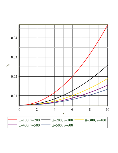
Figure 1: Graph of metric potential versus r.

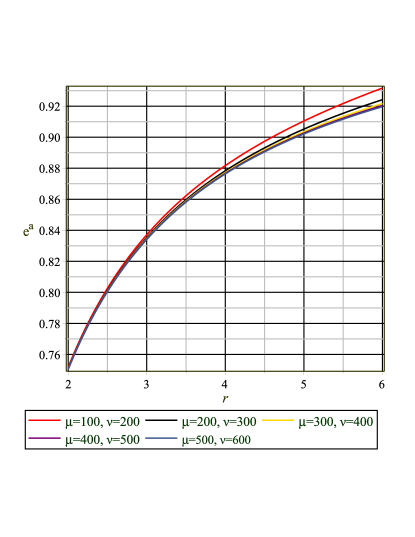
Figure 2: Graph of metric potential versus r.

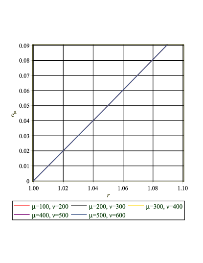
Figure 3: Graph of metric potential versus r.

5 Physical Aspects of Compact Objects

Here, we examine the physical features of compact objects by graphical interpretation of fluid parameters, energy conditions, stability analysis and speed of sound.

5.1 Effective Fluid Parameters

The fluid parameters should be maximum at the center. For this reason, we consider small radii to analyze the smooth behavior of compact stars. The plots of the effective matter variables are given in Figure 4, which shows positive behavior inside the compact object and decreasing nature at the surface boundary. This represents the compact behavior of the star at the center. Furthermore, we examine that the gradient of effective fluid parameters is negative which shows the high compactness of the compact object. Here, we observe that stellar structures depend upon the conserved quantities.

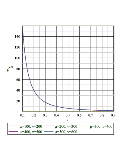
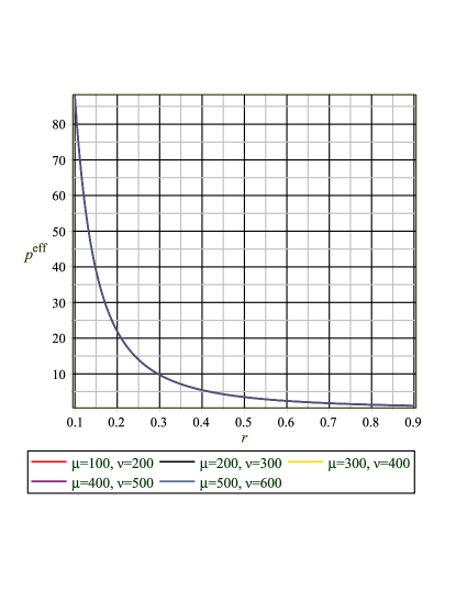
Figure 4: Behavior of effective fluid parameters versus r.

5.2 Energy conditions

The energy bounds are the key aspect in determining the physical presence of cosmic geometries and viable fluid configuration. These bounds must be satisfied for compact objects to have a physically viable geometry. These bounds are the key aspects to investigate the nature of the matter in the compact object determined as [31]

$$\mathbb{NEC}:\quad\mathrm{\rho}^{eff}+\mathrm{p}^{eff}-\textit{A}\geq 0,$$

$$\mathbb{WEC}:\quad\mathrm{\rho}^{eff}-\textit{A}\geq 0,\quad\mathrm{\rho}^{eff}+\mathrm{p}^{eff}-\textit{A}\geq 0,$$

$$\mathbb{SEC}:\quad\mathrm{\rho}^{eff}+\mathrm{p}^{eff}-\textit{A}\geq 0,\quad\mathrm{\rho}^{eff}+3\mathrm{p}^{eff}-\textit{A}\geq 0,$$

$$\mathbb{DEC}:\quad\mathrm{\rho}^{eff}-\textit{A}\geq 0,\quad\mathrm{\rho}^{eff}\pm\mathrm{p}^{eff}-\textit{A}\geq 0,$$

where $\mathbb{NEC}$, $\mathbb{WEC}$, $\mathbb{SEC}$ and $\mathbb{DEC}$ define the null, weak, strong and dominant energy conditions, respectively, while $\textit{A}=\frac{1}{4e^{b}}\left(a^{\prime 2}+2a^{\prime\prime}+4a^{\prime}\emph{r}^{-1}-a^{\prime}b^{\prime}\right)$ is an acceleration term that appears due to the matter source.

The energy density must be positive inside the compact star and maximum at the center for the physically viable geometry. The graphical behavior of energy bounds for various values of $\mu$ and $\nu$ is shown in Figure 5, which shows the viability and consistency of our considered $f(\mathcal{R},\mathcal{T})$ model.

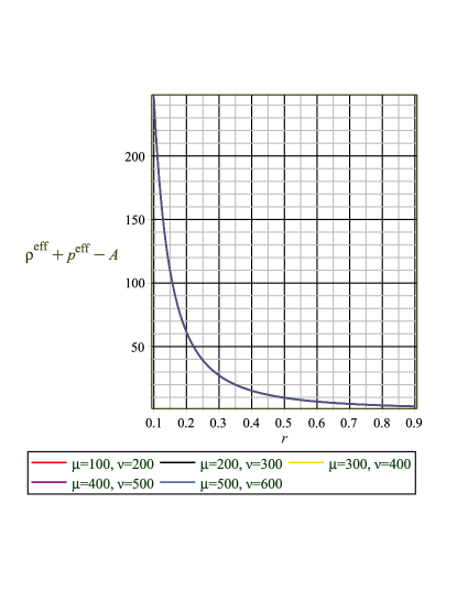
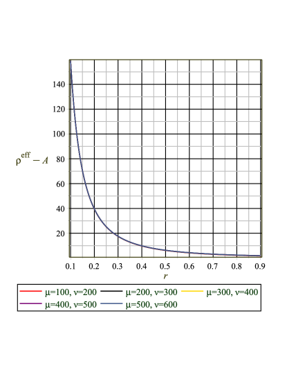
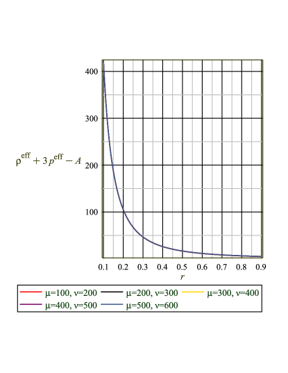
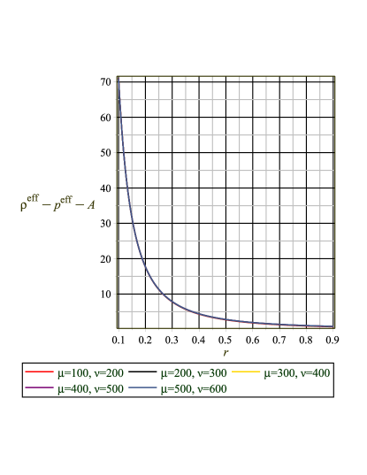
Figure 5: Behavior of energy bounds.

5.3 The Modified TOV Equation

The conserved equation is expressed as

$$\nabla^{\alpha}T^{eff}_{\alpha\beta}=0.$$ (40)

We use a modified TOV equation with dust fluid distribution to examine the equilibrium state of compact objects.

$$-\frac{d\mathrm{p}^{eff}}{d\emph{r}}-\frac{a^{\prime}}{2}(\mathrm{\rho}^{eff}+\mathrm{p}^{eff})=0.$$ (41)

This describes the relation of gravitational $\left(\mathcal{F}_{\mathfrak{g}}\right)$ and hydrostatic $\left(\mathcal{F}_{\mathfrak{h}}\right)$ force that describe the stable state of stellar structure. In the view of Eq.(41), these forces can be divided as $\mathcal{F}_{\mathfrak{g}}=-\frac{a^{\prime}}{2}(\mathrm{\rho}^{eff}+\mathrm{p}^{eff})$ and $\mathcal{F}_{\mathfrak{h}}=-\frac{d\mathrm{p}^{eff}}{d\emph{r}}$. The null impact of these forces $\left(\mathcal{F}_{\mathfrak{h}}+\mathcal{F}_{\mathfrak{g}}=0\right)$ determine the presence of viable compact stars [32]. The graphical behavior of $\mathcal{F}_{\mathfrak{h}}$ and $\mathcal{F}_{\mathfrak{g}}$ for different values of $\mu$ and $\nu$ is presented in Figure 6, which shows the equilibrium state of the stellar system.

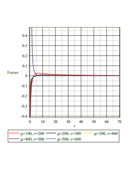
Figure 6: Behavior of hydrostatic and gravitational forces ($\mathcal{F}_{\mathfrak{h}}$, $\mathcal{F}_{\mathfrak{g}}$).

5.4 Stability Analysis

5.4.1 Sound Speed

The physical viability and consistency of a model are dependent on the stability of compact objects. We assume Herrera’s cracking method [33] to examine the stability of our proposed model. This approach stated that sound speed $(v_{s}^{2})$ must satisfy the given condition $(0\leq v_{s}^{2}\leq 1)$ and it is defined as

$$v_{s}^{2}=\frac{d\mathrm{p}^{eff}}{d\mathrm{\rho}^{eff}}.$$ (42)

Figure 7 shows that $v_{s}^{2}$ satisfies the required condition and hence matter configuration is stable.

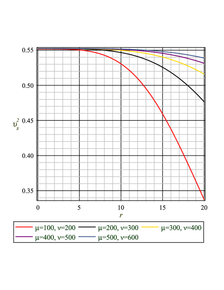
Figure 7: Variation of speed of sound.

5.4.2 Adiabatic Index

Chandrasekhar [34] introduced the formalism to examine the stability of the celestial object against radial perturbation. Many researchers has been established and used this approach on the astrophysical level [35]. The adiabatic index is defined as

$$\Omega=\left(\frac{\mathrm{\rho}^{eff}+\mathrm{p}^{eff}}{\mathrm{p}^{eff}}\right)\left(\frac{d\mathrm{p}^{eff}}{d\mathrm{\rho}^{eff}}\right).$$

For a stable configuration, the adiabatic index should be greater than 4/3 within the isotropic stellar system. The graphical behavior of the adiabatic index is given in Figure 8, which shows that our system is in a stable state.

Figure 8: Graph of adiabatic index corresponding to r.

5.5 Compactness and Surface Redshift

The compactness factor is the ratio of mass and radius of a celestial object. The mass of the star is directly proportional to the radius as shown in Figure 9 and $M(\emph{r})\rightarrow 0$ as $\emph{r}\rightarrow 0$, which determines that the mass is an increasing function and regular at the core of a star. The compactness factor is defined in the following form

$$\gamma=\frac{M(\emph{r})}{\emph{r}}.$$

The gravitational redshift plays a key role to examine the smooth relation between particles in the stellar object. The gravitational redshift is expressed as

$$Z_{s}=\frac{1}{\sqrt{1-2\gamma}}-1.$$

The graphical behavior of the compactness factor and surface redshift is given in Figure 10. These plots manifest that the behavior of $\gamma$ and $Z_{s}$ is increasing as required.

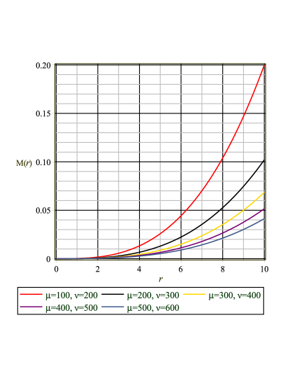
Figure 9: Behavior of the mass function versus r.

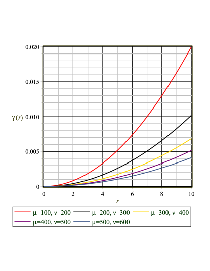
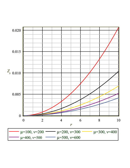
Figure 10: Graphs of the compactness parameter and surface redshift versus r.

6 Concluding Remarks

Noether symmetries are very useful to determine the exact solutions of the physical system. The Lagrange multipliers reduce the complex structure that eventually assists in evaluating the exact solutions. In this article, we have examined the physical features of compact stars through the NS technique. We have established Lagrangian of this theory and formulated symmetry generators and corresponding conserved parameters. The exact solutions of the field equations have been analyzed for a specific model of this theory. The major consequences of this paper are bestowed as follows.

• The metric elements must be positive, finite and non-singular at every point in the geometry of the star to obtain the physically viable model. Figures 1, 2 and 3 shows the viability and the consistency of our metric elements.

• The effective fluid parameters should be maximum at the core of compact objects. The graphs for small radius have been plotted to show the smooth behavior of compact objects. These fluid parameters have a maximum value at the center and decrease towards the boundary that represents the viable behavior (Figure 4).

• All energy constraints are well satisfied for a proposed model which determine the viable matter (Figure 5).

• We have examined the equilibrium state (Figure 6) through TOV equation and found that our model is compatible with stability condition (Figures 7 and 8).

• The graphical analysis of the mass function is found to be increasing and regular at the center of the star (Figure 9).

• Finally, we have found (Figure 10) that the behavior of compactness parameter and gravitational redshift function is increasing as required.

We have concluded that compact objects in this theory through the NS technique depend on the conserved and model parameters. We have investigated that all physical attributes of stellar objects fulfill the physically viable pattern. We found that the NS technique in $f(\mathcal{R},\mathcal{T})$ gravity yields a more realistic and stable model.

References

• [1] Felice, A.D. and Tsujikawa, S.R.: Living Rev. Relativ. 13(2010)3; Nojiri, S. and Odintsov, S.D.: Phys. Rep. 505(2011)59; Bamba, et al.: Astrophys. Space Sci. 342(2012)155.
• [2] Harko, T. and Lobo, F.S.N.: Galaxies 2(2014)410.
• [3] Harko, T. et al.: Phys. Rev. D 84(2011)024020.
• [4] Haghani, Z. et al.: Phys. Rev. D 88(2013)044023.
• [5] Moraes, P.H.R.S. and Santos, J.R.L.: Eur. Phys. J. C 76(2016)60.
• [6] Barrientos, E. et al. Phys. Rev. D 97(2018)104041; Barrientos, E. and Mendoza, S.: Phys. Rev. D 98(2018)084033.
• [7] Capozziello, S., De Laurentis, M. and Odintsov, S.D.: Eur. Phys. J. C 72(2012)1434.
• [8] Basilakos, S., Tsamparlis, M. and Paliathanasis, A.: Phys. Rev. D 83(2011)103512; Paliathanasis, A., Tsamparlis, M. and Basilakos, S.: Phys. Rev. D 84(2011)123514; Basilakos, S. et al.: Phys. Rev. D 88(2013)103526; Paliathanasis, A. et al.: Phys. Rev. D 89(2014)063532.
• [9] Capozziello, S., Stabile, A. and Troisi, A.: Class. Quantum Grav. 25(2008)085004; Roshan, M. and Shojai, F.: Phys. Lett. B 668(2008)238; Cosmol. J.: Astropart. Phys. 2(2013)043; Shamir, M.F. and Ahmad, M.: Eur. Phys. J. C 77(2017)55; Mod. Phys. Lett. A 32(2017)1750086.
• [10] Capozziello, S., Stabile, A. and Troisi, A.: Class. Quantum Grav. 25(2008)085004.
• [11] Roshan, M. and Shojai, F.: Phys. Lett. B 668(2008)238.
• [12] Sharif, M. and Fatima, H.I.: J. Exp. Theor. Phys. 122(2016)104.
• [13] Shamir, M.F. and Ahmad, M.: Eur. Phys. J. C 77(2017)55; Mod. Phys. Lett. A 32(2017)1750086.
• [14] Sharif, M. and Nawazish, I.: J. Exp. Theor. Phys. 120(2014)49; Sharif, M. and Shafique, I.: Phys. Rev. D 90(2014)084033. Sharif, M. and Gul, M.Z.: Eur. Phys. J. Plus 133(2018)345; Int. J. Mod. Phys. D 28(2019)1950054; Chin. J. Phys. 57(2019)329; Int. J. Mod. Phys. A 36(2021)2150004; Chin. J. Phys. 71(2021)365; Universe 07(2021)154; Phys. Scr. 96(2021)105001.
• [15] Sharif, M. and Gul, M.Z.: Phys. Scr. 96(2020)025002.
• [16] Sharif, M. and Gul, M.Z.: Eur. Phys. J. Plus 136(2021)503; Adv. Astron. 2021(2021)6663502.
• [17] Camenzind, M.: Compact Objects in Astrophysics (Springer, Berlin, 2007); Abbas, G., Nazeer, S. and Meraj, M.A.: Astrophys. Space Sci. 354(2014)449; Abbas, G., Kanwal, A. and Zubair, M.: Astrophys. Space Sci. 357(2015)109.
• [18] Abbas, G. et al.: Astrophys. Space Sci. 357(2015)158.
• [19] Zubair, M. and Abbas, G.: Astrophys. Space Sci. 361(2016)342.
• [20] Shamir, M.F. and Naz, N.: Phys. Lett. B 806(2020)135519.
• [21] Astashenok, A.V., Capozziello, S. and Odintsov, S.D.: Phys. Lett. B 742(2015)160.
• [22] Momeni, D.: Int. J. Mod. Phys. A 30(2015)1550093.
• [23] Capozziello, S. et al.: Phys. Rev. D 93(2016)023501.
• [24] Momeni, D. et al.: Int. J. Geom. Methods Mod. Phys. 15(2018)1850091.
• [25] Krori, K.D. and Barua, J.: J. Phys. A 8(1975)508.
• [26] Starobinsky, A. A.: Phys. Lett. B 91(1980)99.
• [27] Ilyas, M. et al.: Astrophys. Space Sci. 362(2017)237.
• [28] Moraes, P.H.R.S., Correa, R.A.C. and Ribeiro, G. arXiv:1701.01027.
• [29] Sharif, M. and Siddiqa, A.: Int. J. Mod. Phys. D 27(2018)1850065. Sharif, M. and Waseem, A.: Eur. Phys. J. C 78(2018)868; Int. J. Mod. Phys. D 2(2019)1950033; Sharif, M. and Gul, M.Z.: Eur. Phys. J. Plus 133(2018)345; Int. J. Mod. Phys. D 28(2019)1950054; Chin. J. Phys. 57(2019)329.
• [30] Capozziello, S,. Stabile, A. and Troisi, A.: Class. Quantum Grav. 24(2007)2153; Capozziello, S., De Laurentis, M. and Stabile, A.: 27(2010)165008.
• [31] Santos, J. et al.: Phys. Rev. D 76(2007)083513.
• [32] Oppenheimer, J.R. and Volkoff, G.M.: Phys. Rev. 55(1939)374; Tolman, R.C.: Phys. Rev. 55(1939)364.
• [33] Herrera, L.: Phys. Lett. A 165(1992)206.
• [34] Chandrasekhar, S.: Phys. Rev. Lett. 12(1964)114.
• [35] Bardeen, J.M., Thorne, K.S. and Meltzer, D.W.: Astrophys. J. 145(1966)505; Knutsen, H.: Mon. Not. R. Astron. Soc. 232(1988)163; Mak, M.K. and Harko, T.: Eur. Phys. J. C 73(2013)2585.