SimTeG: A Frustratingly Simple Approach Improves Textual Graph Learning

Abstract

Textual graphs (TGs) are graphs whose nodes correspond to text (sentences or documents), which are widely prevalent. The representation learning of TGs involves two stages: $(i)$ unsupervised feature extraction and $(ii)$ supervised graph representation learning. In recent years, extensive efforts have been devoted to the latter stage, where Graph Neural Networks (GNNs) have dominated. However, the former stage for most existing graph benchmarks still relies on traditional feature engineering techniques. More recently, with the rapid development of language models (LMs), researchers have focused on leveraging LMs to facilitate the learning of TGs, either by jointly training them in a computationally intensive framework (merging the two stages), or designing complex self-supervised training tasks for feature extraction (enhancing the first stage). In this work, we present SimTeG, a frustratingly Simple approach for Textual Graph learning that does not innovate in frameworks, models, and tasks. Instead, we first perform supervised parameter-efficient fine-tuning (PEFT) on a pre-trained LM on the downstream task, such as node classification. We then generate node embeddings using the last hidden states of finetuned LM. These derived features can be further utilized by any GNN for training on the same task. We evaluate our approach on two fundamental graph representation learning tasks: node classification and link prediction. Through extensive experiments, we show that our approach significantly improves the performance of various GNNs on multiple graph benchmarks. Remarkably, when additional supporting text provided by large language models (LLMs) is included, a simple two-layer GraphSAGE trained on an ensemble of SimTeG achieves an accuracy of 77.48% on OGBN-Arxiv, comparable to state-of-the-art (SOTA) performance obtained from far more complicated GNN architectures. Furthermore, when combined with a SOTA GNN, we achieve a new SOTA of $78.04\%$ on OGBN-Arxiv. Our code is publicly available at https://github.com/vermouthdky/SimTeG and the generated node features for all graph benchmarks can be accessed at https://huggingface.co/datasets/vermouthdky/SimTeG.

1 Introduction

Textual Graphs (TGs) offer a graph-based representation of text data where relationships between phrases, sentences, or documents are depicted through edges. TGs are ubiquitous in real-world applications, including citation graphs (Hu et al., 2020; Yang et al., 2016), knowledge graphs (Wang et al., 2021), and social networks (Zeng et al., 2019; Hamilton et al., 2017), provided that each entity can be represented as text. Different from traditional NLP tasks, instances in TGs are correlated with each other, which provides non-trivial and specific information for downstream tasks. In general, graph benchmarks are usually task-specific (Hu et al., 2020), and most TGs are designed for two fundamental tasks: node classification and link prediction. For the first one, we aim to predict the category of unlabeled nodes while for the second one, our goal is to predict missing links among nodes. For both tasks, text attributes offer critical information.

In recent years, TG representation learning follows a two-stage paradigm: $(i)$ upstream: unsupervised feature extraction that encodes text into numeric embeddings, and $(ii)$ downstream: supervised graph representation learning that further transform the embeddings utilizing the graph structure. While Graph Neural Networks (GNNs) have dominated the latter stage, with an extensive body of academic research published, the former stage surprisingly still relies on traditional feature engineering techniques. For example, in most existing graph benchmarks (Hu et al., 2020; Yang et al., 2016; Zeng et al., 2019), node features are constructed using bag-of-words (BoW) or skip-gram (Mikolov et al., 2013). This intuitively limits the performance of downstream GNNs, as it fails to fully capture textual semantics, fostering an increasing number of GNN models with more and more complex structures. More recently, researchers have begun to leverage the power of language models (LMs) for TG representation learning. Their efforts involve $(i)$ designing complex tasks for LMs to generate powerful node representations (Chien et al., 2021); $(ii)$ jointly training LMs and GNNs in a specific framework (Zhao et al., 2022; Mavromatis et al., 2023); or $(iii)$ fusing the architecture of LM and GNN for end-to-end training (Yang et al., 2021). These works focus on novel training tasks, model architectures, or training frameworks, which generally require substantially modifying the training procedure. However, we argue that such complexity is not actually needed. As a response, in this paper, we present a frustratingly simple yet highly effective method that does not innovate in any of the above aspects but significantly improves the performance of GNNs on TGs.

We are curious about several research questions: $(i)$ How much could language models’ features generally improve the learning of GNN: is the improvement specific for certain GNNs? $(ii)$ What kind of language models fits the needs of textual graph representation learning best? $(iii)$ How important are text attributes on various graph tasks: though previous efforts have shown improvement in node classification, is it also beneficial for link prediction, an equivalently fundamental task that intuitively emphasizes more on graph structures? To the end of answering the above questions, we take an initial step forwards by introducing a simple, effective, yet surprisingly neglected method on TGs and empirically evaluating it on two fundamental graph tasks: node classification and link prediction. Intuitively, when omitting the graph structures, the two tasks are equivalent to text classification and text similarity (retrieval) tasks in NLP, respectively. This intuition motivates us to propose our method: SimTeG. We first parameter-efficiently finetune (PEFT) an LM on the textual corpus of a TG with task-specific labels and then use the finetuned LM to generate node representations given its text by removing the head layer. Afterward, a GNN is trained with the derived node embeddings on the same downstream task for final evaluation. Though embarrassingly simple, SimTeG shows remarkable performance on multiple graph benchmarks w.r.t. node classification and link prediction. Particularly, we find several key observations:

❶ Good language modeling could generally improve the learning of GNNs on both node classification and link prediction. We evaluate SimTeG on three prestigious graph benchmarks for either node classification or link prediction, and find that SimTeG consistently outperforms the official features and the features generated by pretrained LMs (without finetuning) by a large margin. Notably, backed with SOTA GNN, we achieve new SOTA performance of $78.02\%$ on OGBN-Arxiv. See Sec. 5.1 and Appendix A1 for details.

❷ SimTeG significantly complements the margin between GNN backbones on multiple graph benchmarks by improving the performance of simple GNNs. Notably, a simple two-layer GraphSAGE (Hamilton et al., 2017) trained on SimTeG with proper LM backbones achieves on-par SOTA performance of $77.48\%$ on OGBN-Arxiv (Hu et al., 2020).

❸ PEFT are crucial when finetuning LMs to generate representative embeddings, because full-finetuning usually leads to extreme overfitting due to its large parameter space and the caused fitting ability. The overfitting in the LM finetuning stage will hinder the training of downstream GNNs with a collapsed feature space. See Sec. 5.3 for details.

❹ SimTeG is moderately sensitive to the selection of LMs. Generally, the performance of SimTeG is positively correlated with the corresponding LM’s performance on text embedding tasks, e.g. classification and retrieval. We refer to Sec. 5.4 for details. Based on this, we expect further improvement of SimTeG once more powerful LMs for text embedding are available.

2 Related Works

In this section, we first present several works that are closely related to ours and further clarify several concepts and research lines that are plausibly related to ours in terms of similar terminology.

Leveraging LMs on TGs. Focusing on leveraging the power of LMs to TGs, there are several works that are existed and directly comparable with ours. For these works, they either focus on $(i)$ designing specific strategies to generate node embeddings using LMs (He et al., 2023; Chien et al., 2021) or $(ii)$ jointly training LMs and GNNs within a framework (Zhao et al., 2022; Mavromatis et al., 2023). Representatively, for the former one, Chien et al. (2021) proposed a self-supervised graph learning task integrating XR-Transformers (Zhang et al., 2021b) to extract node representation, which shows superior performance on multiple graph benchmarks, validating the necessity for acquiring high-quality node features for attributed graphs. Besides, He et al. (2023) utilizes ChatGPT (OpenAI, 2023) to generate additional supporting text with LLMs. For the latter mechanism, Zhao et al. (2022) proposed a variational expectation maximization joint-training framework for LMs and GNNs to learn powerful graph representations. Mavromatis et al. (2023) designs a graph structure-aware framework to distill the knowledge from GNNs to LMs. Generally, the joint-training framework requires specific communication between LMs and GNNs, e.g. pseudo labels (Zhao et al., 2022) or hidden states (Mavromatis et al., 2023). It is worth noting that the concurrent work He et al. (2023) proposed a close method to ours. However, He et al. (2023) focuses on generating additional informative texts for nodes with LLMs, which is specifically for citation networks on node classification task. In contrast, we focus on generally investigating the effectiveness of our proposed method, which could be widely applied to unlimited datasets and tasks. Utilizing the additional text provided by He et al. (2023), we further show that our method could achieve now SOTA on OGBN-Arxiv. In addition to the main streams, there are related works trying to fuse the architecture of LM and GNN for end-to-end training. Yang et al. (2021) proposed a nested architecture by injecting GNN layers into LM layers. However, due to the natural incompatibleness regarding training batch size, this architecture only allows $1$-hop message passing, which significantly reduce the learning capability of GNNs.

More “Related” Works. ❶ Graph Transformers (Wu et al., 2021; Ying et al., 2021; Hussain et al., 2022; Park et al., 2022; Chen et al., 2022): Nowadays, Graph Transformers are mostly used to denote Transformer-based architectures that embed both topological structure and node features. Different from our work, these models focus on graph-level problems (e.g. graph classification and graph generation) and specific domains (e.g. molecular datasets and protein association networks), which cannot be adopted on TGs. ❷ Leveraging GNNs on Texts (Zhu et al., 2021; Huang et al., 2019; Zhang et al., 2020): Another seemingly related line on integrating GNNs and LMs is conversely applying GNNs to textual documents. Different from TGs, GNNs here do not rely on ground-truth graph structures but the self-constructed or synthetic ones.

3 Preliminaries

Notations. To make notations consistent, we use bold uppercase letters to denote matrices and vectors, and calligraphic font types (e.g. $\mathcal{T}$) to denote sets. We denote a textual graph as a set $\mathcal{G}=(\mathcal{V},\mathcal{E},\mathcal{T})$, where $\mathcal{V}$ and $\mathcal{E}$ are a set of nodes and edges, respectively. $\mathcal{T}$ is a set of text and each textual item is aligned with a node $v\in\mathcal{V}$. For practical usage, we usually rewrite $\mathcal{E}$ into $\mathbf{A}\in\{0,1\}^{|\mathcal{V}|\times|\mathcal{V}|}$, which is a sparse matrix, where entry $\mathbf{A}_{i,j}$ denotes the link between node $v_{i},v_{j}\in\mathcal{V}$.

Problem Formulations. We focus on two fundamental tasks in TGs: $(i)$ node classification and $(ii)$ link prediction. For node classification, given a TG $\mathcal{G}$, we aim to learn a model $\Phi:\mathcal{V}\rightarrow\mathcal{Y}$, where $\mathcal{Y}$ is the ground truth labels. For link prediction, given a TG $\mathcal{G}$, we aim to learn a model $\Phi:\mathcal{V}\times\mathcal{V}\rightarrow\{0,1\}$, where $f(v_{i},v_{j})=1$ if there is a link between $v_{i}$ and $v_{j}$, otherwise $f(v_{i},v_{j})=0$. Different from traditional tasks that are widely explored by the graph learning community, evolving original text into learning is non-trivial. Particularly, when ablating the graphs structure, node classification and link prediction problem are collapsed to text classification and text similarity problem, respectively. This sheds light on how to leverage LMs for TG representation learning.

Node-level Graph Neural Networks. Nowadays, GNNs have dominated graph-related tasks. Here we focus on GNN models working on node-level tasks (i.e. node classification and link prediction). These models work on generating node representations by recursively aggregating features from their multi-hop neighbors, which is usually noted as message passing. Generally, one can formulate a graph convolution layer as: ${\bm{X}}_{l+1}=\Psi_{l}({\bm{C}}{\bm{X}}_{l})$, where ${\bm{C}}$ is the graph convolution matrix (e.g. ${\bm{C}}={\bm{D}}^{-1/2}{\bm{A}}{\bm{D}}^{-1/2}$ in Vanilla GCN (Kipf & Welling, 2016)) and $\Psi_{l}$ is the feature transformation matrix. For the node classification problem, a classifier (e.g., an MLP) is usually appended to the output of a $k$-layer GNN model; while for link prediction, a similarity function is applied to the final output to compute the similarity between two node embeddings. As shown above, as GNNs inherently evolve the whole graph structure for convolution, it is notoriously challenging for scaling it up. It is worth noting that evolving sufficient neighbors during training is crucial for GNNs. Many studies (Duan et al., 2022; Zou et al., 2019) have shown that full-batch training generally outperforms mini-batch for GNNs on multi graph benchmarks. In practice, the lower borderline of batch size for training GNNs is usually thousands. However, when applying it to LMs, it makes the GNN-LM end-to-end training intractable, as a text occupies far more GPU memories than an embedding.

Text Embeddings and Language Models. Transforming text in low-dimensional dense embeddings serves as the upstream of textual graph representation learning and has been widely explored in the literature. To generate sentence embeddings with LMs, two commonly-used methods are $(i)$ average pooling (Reimers & Gurevych, 2019) by taking the average of all word embeddings along with attention mask and $(ii)$ taking the embedding of the [CLS] token (Devlin et al., 2018). With the development of pre-trained language models (Devlin et al., 2018; Liu et al., 2019), particular language models (Li et al., 2020; Reimers & Gurevych, 2019) for sentence embeddings have been proposed and shown promising results in various benchmarks (Muennighoff et al., 2022).

4 SimTeG: Methodology

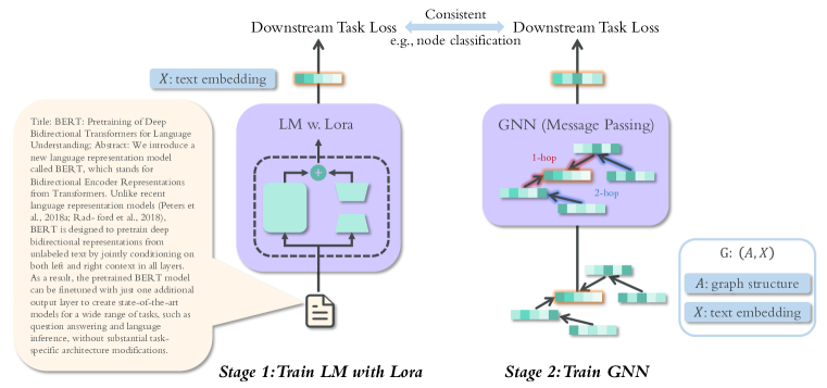
Figure 1: The overview of SimTeG. In stage 1, we train a LM with lora (Hu et al., 2022) and then generate the embeddings ${\bm{X}}$ as the representation of text. In stage 2, we train a GNN on top of the embeddings ${\bm{X}}$, along with the graph structure. The two stages are guided with consistent loss function, e.g., link prediction or node classification.

We propose an extremely simple two-stage training manner that decouples the training of $gnn(\cdot)$ and $lm(\cdot)$. We first finetune $lm$ on $\mathcal{T}$ with the downstream task loss:

$$Loss_{cls}=\mathcal{L}_{\theta}\big{(}\phi(lm(\mathcal{T})),\mathbf{Y}\big{)},\quad Loss_{link}=\mathcal{L}_{\theta}\big{(}\phi\big{(}lm(\mathcal{T}_{src}),lm(\mathcal{T}_{dst})\big{)},\mathbf{Y}\big{)},$$ (1)

where $\phi(\cdot)$ is the classifier (left for node classification) or similarity function (right for link prediction) and $\mathbf{Y}$ is the label. After finetuning, we generate node representations ${\bm{X}}$ with the finetuned LM $\hat{lm}$. In practice, we follow Reimers & Gurevych (2019) to perform mean pooling over the output of the last layer of the LM and empirically find that such a strategy is more stable and converges faster than solely taking the <cls> token embedding as representation (Zhao et al., 2022). In the second stage, we train $gnn$ on $({\bm{A}},{\bm{X}})$ with the same task. The corresponding loss is computed by replacing $lm(\mathcal{T})$ with $gnn({\bm{A}},{\bm{X}})$. The two stage is fully decoupled and one can take advantage of any existing GNN and LM models. We illustrate the two stages in Fig. 1 and the pseudo code is presented in Appendix A2.1.

Regularization with PEFT. When fully finetuning a LM, the inferred features are prone to overfit the training labels, which results in collapsed feature space and thus hindering the generalization in GNN training. Though PEFT was proposed to accelerate the finetuning process without loss of performance, in our two-stage finetuning stage, we empirically find PEFT (Hu et al., 2022; Houlsby et al., 2019; He et al., 2022) could alleviate the overfitting issue to a large extent and thus provide well-regularized node features. See Sec. 5.3 for empirical analysis. In this work, We take the popular PEFT method, lora (Hu et al., 2022), as the instantiation.

Selection of LM. As the revolution induced by LMs, a substantial number of valuable pre-trained LMs have been proposed. As mentioned before, when ablating graph structures of TG, the two fundamental tasks, node classification and link prediction, are simplified into two well-established NLP tasks, text classification and text similarity (retrieval). Based on this motivation, we select LMs pretrained for information retrieval as the backbone of SimTeG. Concrete models are selected based on the benchmark MTEB considering the model size and the performance on both retrieval and classification tasks. An ablation study regarding this motivation is presented in Sec. 5.4.

A Finetuned LM Provides A More Distinguishable Feature Space. We plot the two-dimensional feature space computed by T-SNE (Van der Maaten & Hinton, 2008) of ${\bm{X}}$-SimTeG, ${\bm{X}}$-Fix (features generated by pretrained LM without finetuning), and ${\bm{X}}$-OGB regarding labels on OGBN-Arxiv and OGBN-Products in Fig. 2. In detail, we randomly select 100 nodes each with various labels and use T-SNE to compute its two-dimensional features. As shown below, ${\bm{X}}$-SimTeG has a significantly more distinguishable feature space as it captures more semantic information and is finetuned on the downstream dataset. Besides, we find that ${\bm{X}}$-Fix is more distinguishable than ${\bm{X}}$-OGB, which illustrates the inner semantic capture ability of LMs. Furthermore, in comparison with OGBN-Arixv, features in OGBN-Products is visually indifferentiable, indicating the weaker correlation between semantic information and task-specific labels. It accounts for the less improvement of SimTeG on OGBN-Products in Sec. 5.1.

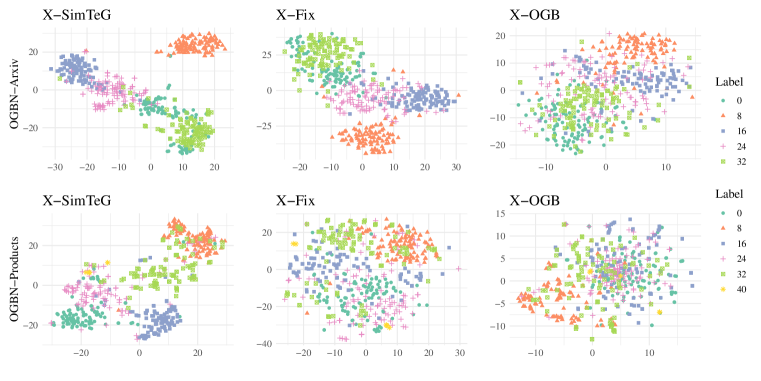
Figure 2: The two-dimensional feature space of ${\bm{X}}$-SimTeG, ${\bm{X}}$-Fix, and ${\bm{X}}$-OGB for OGBN-Arixv, and OGBN-Products. different values and shapes refer to different labels on the specific dataset. The feature values are computed by T-SNE. The LM backbone is e5-large.

5 Experiments

In the experiments, we aim at answering three research questions as proposed in the introduction (Sec. 1). For a clear statement, we split and reformat them into the following research questions. Q1: How much could SimTeG generally improve the learning of GNNs on node classification and link prediction? Q2: Does X-SimTeG facilitate better convergence for GNNs? Q3: Is PEFT a necessity for LM finetuning stage? Q4: How sensitive is GNN training sensitive to the selection of LMs?

Datasets. Focusing on two fundamental tasks node classification and link prediction, we conduct experiments on three prestigious benchmarks: OGBN-Arxiv (Arxiv), OGBN-Products (Products), and OGBL-Citation2 (Hu et al., 2020). The former two are for node classification while the latter one is for link prediction. For the former two, we follow the public split, and all text resources are provided by the officials. For the latter one, OGBL-Citation2, as no official text resources are provided, we take the intersection of it and another dataset ogbn-papers100M w.r.t. unified paper ids, which results in a subset of OGBL-Citation2 with about 2.7M nodes. The public split is further updated according to this subset. In comparison, the original OGBL-Citation2 has about 2.9M nodes, which is on par with the TG version, as the public valid and test split occupies solely 2% overall. As a result, we expect roughly consistent performance for methods on the TG version of OGBL-Citation2 and the original one. We introduce the statistics of the three datasets in Table. A8 and the details in Appendix A2.2.

Baselines. We compare SimTeG with the official features ${\bm{X}}$-OGB (Hu et al., 2020), which is the mean of word embeddings generated by skip-gram (Mikolov et al., 2013). In addition, for node classification, we include another two SOTA methods: ${\bm{X}}$-GIANT (Chien et al., 2021) and GLEM (Zhao et al., 2022). Particularly, ${\bm{X}}$-* are methods are different at learning node embeddings and any GNN model could be applied in the downstream task for a fair comparison. To make things consistent, we denote our method as ${\bm{X}}$-SimTeG without further specification.

GNN Backbones. Aiming at investigating the general improvement of SimTeG, for each dataset, we select two commonly-used baselines GraphSAGE and MLP besides one corresponding SOTA GNN models based on the official leaderboard. For OGBN-Arxiv, we select RevGAT (Li et al., 2021); for OGBN-Products, we select SAGN+SCR (Sun et al., 2021; Zhang et al., 2021a); and for ogbn-citation2, we select SEAL (Zhang & Chen, 2018).

LM Backbones. For retrieval LM backbones, we select three popular LMs on MTEB (Muennighoff et al., 2022) leaderboard w.r.t. model size and performance on classification and retrieval: all-MiniLM-L6-v2 (Reimers & Gurevych, 2019), all-roberta-large-v1 (Reimers & Gurevych, 2019), and e5-large-v1 (Wang et al., 2022). We present the properties of the three LMs in Table. A10.

Hyperparameter search. We utilize optuna (Akiba et al., 2019) to perform hyperparameter search on all tasks. The search space for LMs and GNNs on all datasets is presented in Appendix A2.4.

5.1 Q1: How much could SimTeG generally improve the learning of GNNs on node classification and link prediction?

In this section, we conduct experiments to show the superiority of SimTeG on improving the learning of GNNs on node classification and link prediction. The reported results are selected based on the validation dataset. We present the results based on e5-large backbone in Table. 1 and present the comprehensive results of node classification and link prediction with all the three selected backbones in Table A5 and Table A6. Specifically, in Table 1, we present two comparison metric $\Delta_{\textit{MLP}}$ and $\Delta_{\textit{GNN}}$ to describe the performance margin of (SOTA GNN, MLP) (SOTA GNN, GraphSAGE), respectively. The smaller the value is, even negative, the better the performance of simple models is. In addition, we ensemble the GNNs with multiple node embeddings generated by various LMs and text resources on OGBN-Arxiv and show the results in Table 2. We find several interesting observations as follows.

Table 1: The performance of SOTA GNN, GraphSAGE and MLP on OGBN-Arxiv, OGBN-Products, OGBL-Citation2, which are averaged over $10$ runs (Please note the we solely train LM once to generate the node embeddings). The results of GLEM is from the orignal paper. We bold the best results w.r.t. the same GNN backbone and red color the smallest $\Delta_{\textit{MLP}}$ and $\Delta_{\textit{GNN}}$.

Dataset	Metric	Method	SOTA GNN	A $2$-layer Simple MLP / GNN
			RevGAT	MLP	$\Delta_{\textit{MLP}}$	GraphSAGE	$\Delta_{\textit{GNN}}$
Arxiv	Acc. (%)	${\bm{X}}$-OGB	74.01 $\pm$ 0.29	47.73 $\pm$ 0.29	25.24	71.80 $\pm$ 0.20	3.40
		${\bm{X}}$-GIANT	75.93 $\pm$ 0.22	71.08 $\pm$ 0.22	4.85	73.70 $\pm$ 0.09	2.23
		GLEM	76.97 $\pm$ 0.19	-	-	75.50 $\pm$ 0.24	1.47
		${\bm{X}}$-SimTeG	77.04 $\pm$ 0.13	74.06 $\pm$ 0.13	2.98	76.84 $\pm$ 0.34	0.20
Dataset	Metric	Method	SOTA GNN	A $2$-layer Simple MLP / GNN
			SAGN+SCR	MLP	$\Delta_{\textit{MLP}}$	GraphSAGE	$\Delta_{\textit{GNN}}$
Products	Acc. (%)	${\bm{X}}$-OGB	81.82 $\pm$ 0.44	50.86 $\pm$ 0.26	30.96	78.81 $\pm$ 0.23	3.01
		${\bm{X}}$-GIANT	86.12 $\pm$ 0.34	77.58 $\pm$ 0.24	8.54	82.84 $\pm$ 0.29	3.28
		GLEM	87.36 $\pm$ 0.07	-	-	83.16 $\pm$ 0.19	4.20
		${\bm{X}}$-SimTeG	85.40 $\pm$ 0.28	76.73 $\pm$ 0.44	8.67	84.59 $\pm$ 0.44	0.81
Dataset	Metric	Method	SOTA GNN	A $2$-layer Simple MLP / GNN
			SEAL	MLP	$\Delta_{\textit{MLP}}$	GraphSAGE	$\Delta_{\textit{GNN}}$
Citation2	MRR (%)	${\bm{X}}$-OGB	86.14 $\pm$ 0.40	25.44 $\pm$ 0.01	60.70	77.31 $\pm$ 0.90	8.83
		${\bm{X}}$-SimTeG	86.66 $\pm$ 1.21	72.90 $\pm$ 0.14	13.76	85.13 $\pm$ 0.73	1.53
	Hits@3 (%)	${\bm{X}}$-OGB	90.92 $\pm$ 0.32	28.22 $\pm$ 0.02	62.70	85.56 $\pm$ 0.69	5.36
		${\bm{X}}$-SimTeG	91.42 $\pm$ 0.19	80.55 $\pm$ 0.13	10.87	91.62 $\pm$ 0.87	-0.20

Observation 1: SimTeG generally improves the performance of GNNs on node classification and link prediction by a large margin. As shown in Table 1, SimTeG consistently outperforms the original features on all datasets and backbones. Besides, in comparison with ${\bm{X}}$-GIANT, a LM pretraining method that utilizes the graph structures, SimTeG still achieves better performance on OGBN-Arxiv with all backbones and on OGBN-Products with GraphSAGE, which further indicates the importance of text attributes per se.

Observation 2: (${\bm{X}}$-SimTeG + GraphSAGE) consistently outperforms (${\bm{X}}$-OGB + SOTA GNN) on all the three datasets. This finding implies that the incorporation of advanced text features can bypass the necessity of complex GNNs, which is why we perceive our method to be frustratingly simple. Furthermore, when replacing GraphSAGE with the corresponding SOTA GNN in ${\bm{X}}$-SimTeG, although the performance is improved moderately, this margin of improvement is notably smaller compared to the performance gap on ${\bm{X}}$-OGB. Particularly, we show that the simple 2-layer GraphSAGE achieves comparable performance with the dataset-specific SOTA GNNs. Particularly, on OGBN-Arxiv, GraphSAGE achieves $76.84\%$, taking the 4-th place in the corresponding leaderboard (by 2023-08-01). Besides, on OGBL-Citation2, GraphSAGE even outperforms the SOTA GNN method SEAL on Hits@3.

Observation 3: With additional text attributes, SimTeG with Ensembling achieves new SOTA performance on OGBN-Arxiv. We further demonstrate the effectiveness of SimTeG by ensembling the node embeddings generated by different LMs and texts. For text, we use both the original text provided by Hu et al. (2020) and the additional text attributes provided by He et al. (2023), which is generated by ChatGPT. For LMs, we use both e5-large and all-roberta-large-v1. We train GraphSAGE or RevGAT on those node embeddings generated by various LMs and texts, and make the final predictions with weighted ensembling (taking the weighted average of all predictions). As shown in Table 2, with RevGAT, we achieve new SOTA performance on OGBN-Arxiv with 78.03% test accuracy, more than 0.5 % higher than the previous SOTA performance (77.50%) achieved by He et al. (2023). It further validates the importance of text features and the effectiveness of SimTeG.

Table 2: The performance of GraphSAGE and RevGAT trained on OGBN-Arxiv with additional text attributes provided by He et al. (2023). LMs for ensembling are e5-large and all-roberta-large-v1. We select the top-3 SOTA methods from the leaderboard of OGBN-Arxiv (accessed on 2023-07-18) for comparison and gray color our results (reported over 10 runs).

. Rank Method GNN Backbone Valid Acc. (%) Test Acc. (%) 1 TAPE + SimTeG (ours) RevGAT 78.46 $\pm$ 0.04 78.03 $\pm$ 0.07 2 TAPE (He et al., 2023) RevGAT 77.85 $\pm$ 0.16 77.50 $\pm$ 0.12 3 TAPE + SimTeG (Ours) GraphSAGE 77.89 $\pm$ 0.08 77.48 $\pm$ 0.11 4 GraDBERT (Mavromatis et al., 2023) RevGAT 77.57 $\pm$ 0.09 77.21 $\pm$ 0.31 5 GLEM (Zhao et al., 2022) RevGAT 77.46 $\pm$ 0.18 76.94 $\pm$ 0.25

Observation 4: Text attributes are unequally important for different datasets. As shown in Table 1, we compute $\Delta_{\textit{MLP}}$ which is the performance gap between MLP and SOTA GNNs. Empirically, this value indicates the importance of text attributes on the corresponding dataset, as MLP is solely trained on the texts (integrated with SOTA LMs) while SOTA GNN additionally takes advantage of graph structures. Therefore, approximately, the less $\Delta_{\textit{MLP}}$ is, the more important text attributes are. As presented in Table 1, $\Delta_{\textit{MLP}}$ on OGBN-Arxiv is solely $2.98$, indicating the text attributes are more important, in comparison with the ones in OGBN-Products and OGBL-Citation2. This empirically indicates why the performance of SimTeG in OGBN-Products does not perform as well as the one in OGBN-Arxiv. We show a sample of text in OGBN-Arxiv and OGBN-Products respectively in Appendix A2.2. We find that the text in OGBN-products resembles more a bag of words, which account for the less improvement when using LM features.

5.2 Q2: Does X-SimTeG facilitate better convergence for GNNs?

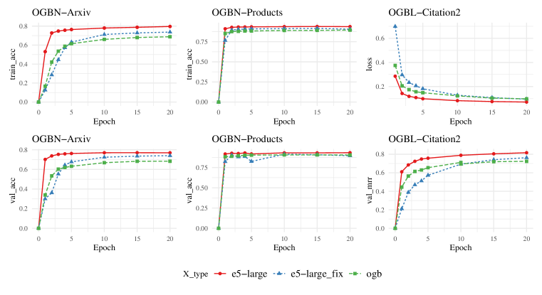
Figure 3: Training convergence and validation results of GNNs with ${\bm{X}}$-SimTeG, ${\bm{X}}$-OGB, and ${\bm{X}}$-FIX. The LM backbone is e5-large. The learning rate and batch size are consistent.

Towards a comprehensive understanding of the effectiveness of SimTeG, we further investigate the convergence of GNNs with SimTeG. We compare the training convergence and the corresponding validation performance of GNNs trained on SimTeG, ${\bm{X}}$-OGB, and ${\bm{X}}$-FIX, where ${\bm{X}}$-FIX denotes the node embeddings generated by the pretrained LMs without finetuning. The illustration is placed in Fig. 3. It is worth noting that we use the training accuracy on OGBN-Arxiv and OGBN-Products to denote their convergence since we utilize label smoothing during training which make the training loss not directly comparable on them. Based on Fig. 3, we have the following observation:

Observation 5: SimTeG moderately speeds up and stabilizes the training of GNNs. As shown in Fig. 3, GNNs with SimTeG generally converge faster than the ones with ${\bm{X}}$-OGB and ${\bm{X}}$-FIX. With SimTeG, GraphSAGE could converge within 2 epochs on OGBN-Arxiv and OGBN-Products. In contrast, training on the features directly generated by the pretrained LMs (i.e., ${\bm{X}}$-FIX) converges much slower, even slower than one of ${\bm{X}}$-OGB (possibly due to a larger hidden dimension). This further indicates the benefits of SimTeG.

5.3 Q3: Is PEFT a necessity for LM finetuning stage?

In this ablation study, we analyze the effectiveness of PEFT for LM finetuning stage in SimTeG. Besides the accelerating finetuning, we also find notable contribution of PEFT to the effectiveness. We summarize the training, validation, and test accuracy of two stages: LM finetuning stage and GNN training stage. The results of node classification are presented in Table 3.

Table 3: The training results of finetuning LM (LM stage) and further training GNN on top of derived features (GNN stage). We compare the results of PEFT (SimTeG) with full-finetuning (${\bm{X}}$-FULL). The LM backbone is e5-large and the GNN backbone is GraphSAGE. We bold the better results on each comparison. $\Delta_{\textit{overfit}}$ computes (Train Acc. - Test Acc.) to measure the overfitting.

datasets	Stage	X_type	Train Acc.	Valid Acc	Test Acc.	$\Delta_{\textit{overfit}}$
Arxiv	LM	${\bm{X}}$-FULL	82.33	75.85	74.77	7.56
		${\bm{X}}$-SimTeG	75.72	75.40	74.31	1.41
	GNN	${\bm{X}}$-FULL	84.39	76.73	75.28	9.11
		${\bm{X}}$-SimTeG	79.37	77.47	76.85	2.52
Products	LM	${\bm{X}}$-FULL	95.46	91.70	78.70	16.76
		${\bm{X}}$-SimTeG	89.45	88.85	77.81	11.64
	GNN	${\bm{X}}$-FULL	96.42	93.18	81.80	14.62
		${\bm{X}}$-SimTeG	95.37	93.57	84.58	10.79

Observation 6: PEFT could significantly alleviate the overfitting problem during finetuning LM and further facilitate the training of GNNs with regularized features. As shown in Table 3, due to the excessively strong learning capacity of LMs, finetuning LMs on the downstream task causes a severe overfitting problem. Although full-finetuning outperforms PEFT in LM stage, training GNNs on the derived features gains notably less improvement. In contrast, PEFT could significantly mitigate the overfitting issue according to $\Delta_{\textit{overfit}}$ in LM finetuning stage and assist the training of GNNs with regularized features to gain considerable improvement compared with full-finetuning.

5.4 Q4: How sensitive is GNN training sensitive to the selection of LMs?

In this experiment, we investigate the effects of the selection of LMs. In detail, we aim at answering two questions: $(i)$ Is the training of GNN sensitive to the selection of LMs? $(ii)$ is retrieval LM a better choice than generally pretrained LMs, e.g. masked language modeling (MLM)? To answer the above questions, we conduct experiments on multiple LM backbones. Particularly, to answer the second question, besides the three retrieval LMs introduced in Table A10, we also consider a LM pretrained with MLM, i.e., roberta-large (Liu et al., 2019), which has exactly the same architecture with all-roberta-large-v1. Based on the results, we have the following observations.

Table 4: The performance of GraphSAGE and MLP trained on SimTeGwith different LM backbones. The former three LMs are finetuned with searched hyperparameters. For each row, we bold the best result and underline the runner-up. all results are reported based on 10 runs.

datasets	Metric	LM backbone	all-MiniLM-L6-v2	all-roberta-large-v1	e5-large
		#Params.	22M	355M	335M
Arxiv	Acc.	MLP	70.56 $\pm$ 0.09	74.32 $\pm$ 0.12	74.06 $\pm$ 0.13
		GraphSAGE	75.14 $\pm$ 0.30	76.18 $\pm$ 0.37	76.84 $\pm$ 0.34
Products	Acc.	MLP	72.36 $\pm$ 0.12	77.48 $\pm$ 0.19	76.73 $\pm$ 0.44
		GraphSAGE	82.04 $\pm$ 0.57	83.68 $\pm$ 0.32	84.59 $\pm$ 0.44
Citation2	MRR	MLP	64.49 $\pm$ 0.18	70.32 $\pm$ 0.22	72.90 $\pm$ 0.14
		GraphSAGE	83.09 $\pm$ 0.75	85.29 $\pm$ 0.70	85.13 $\pm$ 0.73

Observation 7: GNN’s training is moderately sensitive to the selection of LMs. We select three retrieval LMs based on their rank in MTEB leaderboard in terms of the classification and retrieval performance. Interestingly, based on the leaderboard, the performance ranking is e5-large $>$ all-roberta-large-v1 $>$ all-MiniLM-L6-v2, which is consistent with their overall performance in Table 4. We conjecture that with more powerful retrieval LMs, the performance of GNNs will be further improved. In addition, we perform an ablation study regarding the comparison between retrieval LMs and MLM LMs. The results are shown in Table A7. We observe that given the same architecture, the models specifically pretrained for retrieval tasks (all-roberta-large-v1) generally perform better on tasks of TG representation learning.

6 Conclusion

In this work, we propose a frustratingly simple, yet highly effective approach SimTeG for TG representation learning. We show that with a parameter-efficiently finetuned LM on the same downstream task first, a simple two-layer GraphSAGE trained on the generated node embeddings can achieve on-par state-of-the-art (SOTA) performance on OGBN-Arxiv (77.48 %). Furthermore, with SOTA GNN, we achieve new SOTA of $78.04\%$ on OGBN-Arxiv. It is worth noting this simple baseline complements any LMs and GNNs, and we expect further performance improvement given more powerful LMs and GNNs.

Appendix A1 More Experiment Results

Table A5: Node Classification Accuracy of $\mathbf{X}$-SimTeG on ogbn-arxiv (Arxiv) and ogbn-products (Products). All reported results are averaged over $10$ runs in the format of mean $\pm$ std. We red color the best results and blue color the runner-ups with the same GNN backbone. $\uparrow(\%)$ denotes the improvement of $\mathbf{X}$-SimTeG over the original feature ${\bm{X}}$-OGB. $\Delta_{\textit{MLP}}$ and $\Delta_{\textit{GNN}}$ denotes the extreme value difference among all methods (including MLP) and GNNs, respectively.

Datasets	GNN	Acc. (%)	Baselines			$\mathbf{X}$-SimTeG
			$\mathbf{X}$-OGB	$\mathbf{X}$-GIANT	GLEMa	MiniLM-L6	$\uparrow$ (%)	e5-large	$\uparrow$ (%)	roberta-large	$\uparrow$ (%)
Arxiv	MLP	val	49.14 $\pm$ 0.27	72.02 $\pm$ 0.16	-	71.59 $\pm$ 0.07	22.45	75.08 $\pm$ 0.09	26.66	74.80 $\pm$ 0.07	25.66
		test	47.73 $\pm$ 0.29	71.08 $\pm$ 0.22	-	70.56 $\pm$ 0.09	22.83	74.06 $\pm$ 0.13	26.33	74.32 $\pm$ 0.12	26.59
	GraphSAGE	val	72.80 $\pm$ 0.18	74.58 $\pm$ 0.20	76.45 $\pm$ 0.05	75.92 $\pm$ 0.17	3.12	77.47 $\pm$ 0.14	4.67	76.86 $\pm$ 0.13	4.06
		test	71.80 $\pm$ 0.20	73.70 $\pm$ 0.09	75.50 $\pm$ 0.24	75.14 $\pm$ 0.30	3.34	76.84 $\pm$ 0.34	5.04	76.18 $\pm$ 0.37	4.38
	GAMLP	val	71.49 $\pm$ 0.41	76.36 $\pm$ 0.09	76.95 $\pm$ 0.14	76.75 $\pm$ 0.11	5.26	77.90 $\pm$ 0.12	6.41	77.57 $\pm$ 0.15	6.08
		test	70.61 $\pm$ 0.52	75.26 $\pm$ 0.15	75.62 $\pm$ 0.23	75.46 $\pm$ 0.17	4.85	76.92 $\pm$ 0.10	6.31	76.72 $\pm$ 0.19	6.11
	SAGN	val	72.74 $\pm$ 0.39	75.76 $\pm$ 0.21	-	76.84 $\pm$ 0.08	4.10	78.03 $\pm$ 0.05	5.29	77.63 $\pm$ 0.16	4.89
		test	71.76 $\pm$ 0.41	74.39 $\pm$ 0.38	-	75.50 $\pm$ 0.23	3.74	76.85 $\pm$ 0.12	5.09	76.59 $\pm$ 0.17	4.83
	RevGAT	val	75.10 $\pm$ 0.15	76.97 $\pm$ 0.08	77.49 $\pm$ 0.17	76.86 $\pm$ 0.24	1.76	77.68 $\pm$ 0.07	2.58	76.32 $\pm$ 0.18	1.22
		test	74.01 $\pm$ 0.29	75.93 $\pm$ 0.22	76.97 $\pm$ 0.19	75.96 $\pm$ 0.21	1.95	77.04 $\pm$ 0.13	3.03	75.88 $\pm$ 0.58	1.87
	$\Delta_{\textit{MLP}}$/$\Delta_{\textit{GNN}}$		25.24 / 3.40	4.85 / 2.23	-	5.40 / 0.82	-	2.98 / 0.20	-	2.40 / 0.84	-
Products	MLP	val	63.44 $\pm$ 0.30	89.67 $\pm$ 0.07	-	86.82 $\pm$ 0.02	23.38	88.75 $\pm$ 0.04	25.31	90.01 $\pm$ 0.03	26.57
		test	50.86 $\pm$ 0.26	77.58 $\pm$ 0.24	-	72.36 $\pm$ 0.12	21.50	76.73 $\pm$ 0.44	25.87	77.48 $\pm$ 0.19	26.62
	GraphSAGE	val	90.03 $\pm$ 0.08	93.49 $\pm$ 0.09	93.84 $\pm$ 0.12	93.49 $\pm$ 0.08	3.46	93.57 $\pm$ 0.20	3.54	93.34 $\pm$ 0.09	3.31
		test	78.81 $\pm$ 0.23	82.84 $\pm$ 0.29	83.16 $\pm$ 0.19	82.04 $\pm$ 0.57	3.23	84.59 $\pm$ 0.44	5.78	83.68 $\pm$ 0.32	4.87
	SAGN+SCR	val	91.83 $\pm$ 0.24	94.04 $\pm$ 0.12	94.00 $\pm$ 0.03	92.89 $\pm$ 0.07	1.06	94.12 $\pm$ 0.10	2.29	94.13 $\pm$ 0.12	2.30
		test	81.82 $\pm$ 0.44	86.12 $\pm$ 0.34	87.36 $\pm$ 0.07	82.43 $\pm$ 0.40	0.61	85.40 $\pm$ 0.28	3.58	85.23 $\pm$ 0.32	3.41
	$\Delta_{\textit{MLP}}$/$\Delta_{\textit{GNN}}$		30.96 / 3.01	8.54 / 3.28	-	10.07 / 0.39		8.67 / 0.81	-	7.75 / 1.55	-
a results are from the original papers.

Table A6: Link prediction results on OGBL-Citation2-2.7M (Citation2). All reported results are averaged over 5 runs. We red color the best results and blue color the runner-ups with the same GNN backbone. $\uparrow(\%)$ denotes the improvement of $\mathbf{X}$-SimTeG over the original feature ${\bm{X}}$-OGB. $\Delta_{\textit{MLP}}$ and $\Delta_{\textit{GNN}}$ denotes the margin of (MLP, SEAL) and (GraphSAGE, SEAL), respectively. We use blue color denoting the negative values and red denoting positive. Specifically, in the context of $\Delta$, positives indicate MLP/GraphSAGE performs better than SEAL.

Metrics	GNN	Split	Baselines	${\bm{X}}$-SimTeG
			${\bm{X}}$-OGB	MiniLM-L6	$\uparrow(\%)$	roberta-large	$\uparrow(\%)$	e5-large	$\uparrow(\%)$
MRR	MLP	val	25.37 $\pm$ 0.09	64.56 $\pm$ 0.15	39.19	70.20 $\pm$ 0.19	44.83	72.79 $\pm$ 0.17	47.42
		test	25.44 $\pm$ 0.01	64.49 $\pm$ 0.18	39.05	70.32 $\pm$ 0.22	44.88	72.90 $\pm$ 0.14	47.46
	GraphSAGE	val	77.40 $\pm$ 0.88	83.13 $\pm$ 0.72	5.73	85.27 $\pm$ 0.78	7.87	85.20 $\pm$ 0.69	7.80
		test	77.31 $\pm$ 0.90	83.09 $\pm$ 0.75	5.78	85.29 $\pm$ 0.70	7.98	85.13 $\pm$ 0.73	7.82
	SEAL	val	87.21 $\pm$ 0.03	88.33 $\pm$ 0.30	1.12	88.29 $\pm$ 0.45	1.08	88.56 $\pm$ 0.38	1.35
		test	86.14 $\pm$ 0.40	86.69 $\pm$ 0.43	0.55	87.02 $\pm$ 0.46	0.88	86.66 $\pm$ 1.21	0.52
	$\Delta_{\textit{MLP}}$/$\Delta_{\textit{GNN}}$		-60.70 / -8.83	-22.20 / -3.60	-	-16.70 /-1.73	-	-13.76 / -1.53	-
Hits@1	MLP	val	15.04 $\pm$ 0.09	52.29 $\pm$ 0.18	37.25	59.46 $\pm$ 0.19	44.42	62.21 $\pm$ 0.23	47.17
		test	15.11 $\pm$ 0.06	52.18 $\pm$ 0.25	37.07	59.66 $\pm$ 0.26	44.55	62.31 $\pm$ 0.19	47.20
	GraphSAGE	val	67.28 $\pm$ 1.20	74.83 $\pm$ 1.02	7.55	77.98 $\pm$ 1.20	10.70	77.73 $\pm$ 0.89	10.45
		test	67.09 $\pm$ 1.25	74.79 $\pm$ 1.10	7.70	77.99 $\pm$ 0.89	10.90	77.66 $\pm$ 0.91	10.57
	SEAL	val	82.76 $\pm$ 0.14	84.35 $\pm$ 0.42	1.59	84.25 $\pm$ 0.79	1.49	84.70 $\pm$ 0.58	1.94
		test	81.74 $\pm$ 0.46	81.40 $\pm$ 0.96	-0.34	82.34 $\pm$ 0.79	0.60	81.15 $\pm$ 2.04	-0.59
	$\Delta_{\textit{MLP}}$/$\Delta_{\textit{GNN}}$		-66.63 / -14.65	-29.22 /-6.61	-	-22.68 / -4.35	-	-18.84 / -3.39	-
Hits@3	MLP	val	28.06 $\pm$ 0.10	72.60 $\pm$ 0.16	44.54	77.56 $\pm$ 0.23	49.50	80.42 $\pm$ 0.15	52.36
		test	28.22 $\pm$ 0.02	72.62 $\pm$ 0.19	44.40	77.66 $\pm$ 0.24	49.44	80.55 $\pm$ 0.13	52.33
	GraphSAGE	val	85.54 $\pm$ 0.69	90.17 $\pm$ 0.61	4.63	91.55 $\pm$ 0.98	6.01	91.72 $\pm$ 0.90	6.18
		test	85.56 $\pm$ 0.69	90.16 $\pm$ 0.51	4.60	91.57 $\pm$ 1.10	6.01	91.62 $\pm$ 0.87	6.06
	SEAL	val	91.36 $\pm$ 0.44	92.00 $\pm$ 0.07	0.64	92.15 $\pm$ 0.19	0.79	91.75 $\pm$ 0.18	0.39
		test	90.92 $\pm$ 0.32	91.42 $\pm$ 0.60	0.50	91.52 $\pm$ 0.56	0.60	91.42 $\pm$ 0.19	0.50
	$\Delta_{\textit{MLP}}$/$\Delta_{\textit{GNN}}$		-62.70 / -5.36	-18.80 / -1.26	-	-13.86 / 0.05	-	-10.87 / 0.20	-
Hits@10	MLP	val	46.73 $\pm$ 0.14	87.62 $\pm$ 0.06	40.89	89.80 $\pm$ 0.20	43.07	91.74 $\pm$ 0.08	45.01
		test	46.59 $\pm$ 0.11	87.57 $\pm$ 0.12	40.98	89.66 $\pm$ 0.14	43.07	91.74 $\pm$ 0.10	45.15
	GraphSAGE	val	94.29 $\pm$ 0.19	96.25 $\pm$ 0.13	1.96	96.61 $\pm$ 0.12	2.32	96.71 $\pm$ 0.09	2.42
		test	94.37 $\pm$ 0.17	96.30 $\pm$ 0.13	1.93	96.64 $\pm$ 0.12	2.27	96.74 $\pm$ 0.11	2.37
	SEAL	val	94.59 $\pm$ 0.14	94.88 $\pm$ 0.25	0.29	95.08 $\pm$ 0.12	0.49	95.08 $\pm$ 0.21	0.49
		test	93.90 $\pm$ 0.49	94.40 $\pm$ 0.07	0.50	93.95 $\pm$ 0.37	0.05	94.54 $\pm$ 0.25	0.64
	$\Delta_{\textit{MLP}}$/$\Delta_{\textit{GNN}}$		-47.31 / -0.47	-6.83 /1.90	-	-4.29 / 2.66	-	-2.80 / 2.20	-

Table A7: The performance of Graph and MLP trained on SimTeG backed with all-roberta-large-v1 and roberta-large, which have the same model architecture and differs from the pretraining strategy. we bold the best results for each comparison in ${\bm{X}}$-Fix and ${\bm{X}}$-SimTeG. all results are reported based on 10 runs

datasets	Metric	X_type	${\bm{X}}$-Fix		${\bm{X}}$-SimTeG
		LM Backbone	roberta-large	all-roberta-large-v1	roberta-large	all-roberta-large-v1
Arxiv	Acc.	MLP	61.15 $\pm$ 0.83	72.58 $\pm$ 0.25	71.55 $\pm$ 0.24	74.32 $\pm$ 0.12
		GraphSAGE	72.15 $\pm$ 0.59	75.51 $\pm$ 0.23	75.48 $\pm$ 0.16	76.18 $\pm$ 0.37
Products	Acc.	MLP	68.14 $\pm$ 0.23	70.10 $\pm$ 0.08	78.45 $\pm$ 0.14	77.48 $\pm$ 0.19
		GraphSAGE	77.65 $\pm$ 0.34	82.38 $\pm$ 0.60	83.56 $\pm$ 0.21	83.68 $\pm$ 0.32
Citation2	MRR	MLP	00.20 $\pm$ 0.01	70.12 $\pm$ 0.12	63.15 $\pm$ 0.20	72.90 $\pm$ 0.14
		GraphSAGE	79.71 $\pm$ 0.27	83.20 $\pm$ 0.40	84.37 $\pm$ 0.34	85.13 $\pm$ 0.73

Appendix A2 Reproducibility Statement

To ensure the reproducibility of our experiments and benefit the community for further research, we provide the source code at https://github.com/vermouthdky/SimTeG and all node features of SimTeG at https://huggingface.co/datasets/vermouthdky/SimTeG.

A2.1 pseudo code of SimTeG

⬇

# f_lm: language model wrapped with PEFT method, f_mlp: mlp model, f_gnn: gnn model

# inputs: A textual graph (adj_t (A), input_ids (T), att_mask (M)) and task-specific labels (Y)

# outputs: node representations

⬇ # Node Classification for T, M, Y in train_loader: X = f_lm(T, M) logits = f_mlp(X) loss = CrossEntropyLoss(logits, Y) loss.backward() lm_optimizer.step() with torch.no_grad(): X = f_lm(T, M) f_mlp.reset_parameters() for A, X, Y in train_loader: X = f_gnn(A, X) logits = f_mlp(X) loss = CrossEntropyLoss(logits, Y) loss.backward() gnn_optimizer.step() ⬇ # Link Prediction for (T_src, T_dst), (M_src, M_dst), Y in train_loader: X_src, X_dst = f_lm((T_src, M_src), (T_dst, M_dst)) logits = f_mlp(X_src, X_dst) loss = BCEWithLogitsLoss(logits, Y) loss.backward() lm_optimizer.step() with torch.no_grad(): X = lm(T, M) f_mlp.reset_parameters() for A, (X_src, X_dst), Y in train_loader: X_src, X_dst = f_gnn(A, (X_src, X_dst)) logits = f_mlp(X_src, X_dst) loss = BCEWithLogitsLoss(logits, Y) loss.backward() gnn_optimizer.step()

Algorithm 1 PyTorch-style code of SimTeG. Left: node classification; Right: link prediction.

A2.2 Details of TG Version for the three OGB datasets

In this section, we present the details of the TG version of OGBN-Arxiv, OGBN-Products, and OGBL-Citation2. The statistics of the three datasets are shown in Table A8 and the text resources are shown in Table A9.

Table A8: Statistics of OGBN-Arxiv, OGBN-Products, and OGBL-Citation2-2.7M

Datasets	#Nodes	#Edges	Avg. Degree	#Task	Metric
OGBN-Arxiv (Arxiv)	$169,343$	$1,166,243$	13.7	node classification	Accuracy
OGBN-Products (Products)	$2,449,029$	$61,859,140$	50.5	node classification	Accuracy
OGBL-Citation2-2.7M (Citation2)	$2,728,032$	$27,731,705$	10.2	link prediction	MRR / Hits

OGBN-Arxiv. OGBN-Arxiv is a directed academic graph, where node denotes papers and edge denotes directed citation. The task is to predict the category of each paper as listed in https://arxiv.org. For its TG version, we use the same split as Hu et al. (2020). The text for each node is its title and abstract. We concatenate them for each node with the format of "title: {title}; abstract: {abstract}" as the corresponding node’s text. For example, "title: multi view metric learning for multi view video summarization; abstract: Traditional methods on video summarization are designed to generate summaries for single-view video records; and thus they cannot fully exploit the redundancy in multi-view video records. In this paper, we present a multi-view metric learning framework for multi-view video summarization that combines the advantages of maximum margin clustering with the disagreement minimization criterion. …"

OGBN-Products. OGBN-Products is a co-purchase graph, where node denotes a product on Amazon and an edge denotes the co-purchase relationship between two products. The task is to predict the category of each product (node classification). We follow the public split as Hu et al. (2020) and the text processing strategy of GLEM (Zhao et al., 2022). For each node, the corresponding text is its item description. For example, "My Fair Pastry (Good Eats Vol. 9)" "Disc 1: Flour Power (Scones; Shortcakes; Southern Biscuits; Salmon Turnovers; Fruit Tart; Funnel Cake; Sweet or Savory; Pte Choux) Disc 2: Super Sweets 4 (Banana Spitsville; Burned Peach Ice Cream; Chocolate Taffy; Acid Jellies; Peanut Brittle; Chocolate Fudge; Peanut Butter Fudge) …"

OGBL-Citation2-2.7M. OGBL-Citation2-2.7M is a citation graph, where nodes denote papers and edges denote the citations. The task is to predict the missing citation among papers (link prediction). All papers are collected by the official from Mircrosoft Academic Graph whereas the text resources are not provided. Though MAG IDs for all papers are provided, we cannot find all corresponding text resources due to the close of MAG project . Hence, we take an intersection of OGBL-Citation2 and OGBN-Papers100M whose text resources are provided by the official, and build a subgraph, namely OGBL-Citation2-2.7M. It contains 93% nodes of OGBL-Citation2 and offers a roughly on-par performance for baselines.

Table A9: The URLs of text resources for ogbn-arxiv, ogbn-products, and OGBL-Citation2.

Dataset	Text Resource URL
OGBN-Arxiv	https://snap.stanford.edu/ogb/data/misc/ogbn_arxiv/titleabs.tsv.gz
OGBN-Products	https://drive.google.com/u/0/uc?id=1gsabsx8KR2N9jJz16jTcA0QASXsNuKnN&export=download
OGBL-Citation2-2.7M	https://drive.google.com/u/0/uc?id=19_hkbBUDFZTvQrM0oMbftuXhgz5LbIZY&export=download

A2.3 Properties of Language Models

Table A10: Statistics of OGBN-Arxiv, OGBN-Products, and OGBL-Citation2-2.7M

Datasets	#Nodes	#Edges	Avg. Degree	#Task	Metric
OGBN-Arxiv (Arxiv)	$169,343$	$1,166,243$	13.7	node classification	Accuracy
OGBN-Products (Products)	$2,449,029$	$61,859,140$	50.5	node classification	Accuracy
OGBL-Citation2-2.7M (Citation2)	$2,728,032$	$27,731,705$	10.2	link prediction	MRR / Hits

A2.4 Hyperparameter Search Space

For language models, we design the hyperparameter (HP) search space as in Table A11. Please note that for link prediction, the label smoothing factor is omitted. For HP searching, we utilize optuna (Akiba et al., 2019) to search the best HPs for each dataset and each model. For LMs, we take 10 trials. For GNNs, we take 20 trials. The final HP setting for LMs and GNNs are placed as shell scripts in our repository.

Table A11: The search space of LMs and GNNs.

LM			GNN
hyperparameter	search space	type	hyperparameter	search space	type
learning rate	[1e-6, 1e-4]	continual	learning rate	[1e-4, 1e-2]	continual
weight decay	[1e-7, 1e-4]	continual	weight decay	[1e-7, 1e-4]	continual
label smoothing	[0.1, 0.7]	continual	label smoothing	[0.1, 0.7]	continual
header dropout	[0.1, 0.8]	continual	dropout	[0.1, 0.8]	continual
lora r	[1, 2, 4, 8]	descrete	num of layers	[2, 3, 4, 6, 8]	descrete
lora alpha	[4, 8, 16, 32]	descrete
lora dropout	[0.1, 0.8]	continual

References

- Akiba et al. (2019) Takuya Akiba, Shotaro Sano, Toshihiko Yanase, Takeru Ohta, and Masanori Koyama. Optuna: A next-generation hyperparameter optimization framework. In Proceedings of the 25th ACM SIGKDD international conference on knowledge discovery & data mining, pp. 2623–2631, 2019.
- Chen et al. (2022) Dexiong Chen, Leslie O’Bray, and Karsten Borgwardt. Structure-aware transformer for graph representation learning. In International Conference on Machine Learning, pp. 3469–3489. PMLR, 2022.
- Chien et al. (2021) Eli Chien, Wei-Cheng Chang, Cho-Jui Hsieh, Hsiang-Fu Yu, Jiong Zhang, Olgica Milenkovic, and Inderjit S Dhillon. Node feature extraction by self-supervised multi-scale neighborhood prediction. arXiv preprint arXiv:2111.00064, 2021.
- Devlin et al. (2018) Jacob Devlin, Ming-Wei Chang, Kenton Lee, and Kristina Toutanova. Bert: Pre-training of deep bidirectional transformers for language understanding. arXiv preprint arXiv:1810.04805, 2018.
- Duan et al. (2022) Keyu Duan, Zirui Liu, Peihao Wang, Wenqing Zheng, Kaixiong Zhou, Tianlong Chen, Xia Hu, and Zhangyang Wang. A comprehensive study on large-scale graph training: Benchmarking and rethinking. In Advances in Neural Information Processing Systems, volume 35, pp. 5376–5389, 2022.
- Hamilton et al. (2017) Will Hamilton, Zhitao Ying, and Jure Leskovec. Inductive representation learning on large graphs. In NeuIPS, pp. 1024–1034, 2017.
- He et al. (2022) Junxian He, Chunting Zhou, Xuezhe Ma, Taylor Berg-Kirkpatrick, and Graham Neubig. Towards a unified view of parameter-efficient transfer learning. In International Conference on Learning Representations, 2022. URL https://openreview.net/forum?id=0RDcd5Axok.
- He et al. (2023) Xiaoxin He, Xavier Bresson, Thomas Laurent, and Bryan Hooi. Explanations as features: Llm-based features for text-attributed graphs. arXiv preprint arXiv:2305.19523, 2023.
- Houlsby et al. (2019) Neil Houlsby, Andrei Giurgiu, Stanislaw Jastrzebski, Bruna Morrone, Quentin De Laroussilhe, Andrea Gesmundo, Mona Attariyan, and Sylvain Gelly. Parameter-efficient transfer learning for nlp. In International Conference on Machine Learning, pp. 2790–2799. PMLR, 2019.
- Hu et al. (2022) Edward J Hu, Yelong Shen, Phillip Wallis, Zeyuan Allen-Zhu, Yuanzhi Li, Shean Wang, Lu Wang, and Weizhu Chen. LoRA: Low-rank adaptation of large language models. In International Conference on Learning Representations, 2022. URL https://openreview.net/forum?id=nZeVKeeFYf9.
- Hu et al. (2020) Weihua Hu, Matthias Fey, Marinka Zitnik, Yuxiao Dong, Hongyu Ren, Bowen Liu, Michele Catasta, and Jure Leskovec. Open graph benchmark: Datasets for machine learning on graphs. Advances in neural information processing systems, 33:22118–22133, 2020.
- Huang et al. (2019) Lianzhe Huang, Dehong Ma, Sujian Li, Xiaodong Zhang, and Houfeng Wang. Text level graph neural network for text classification. arXiv preprint arXiv:1910.02356, 2019.
- Hussain et al. (2022) Md Shamim Hussain, Mohammed J Zaki, and Dharmashankar Subramanian. Global self-attention as a replacement for graph convolution. In Proceedings of the 28th ACM SIGKDD Conference on Knowledge Discovery and Data Mining, pp. 655–665, 2022.
- Kipf & Welling (2016) Thomas N Kipf and Max Welling. Semi-supervised classification with graph convolutional networks. arXiv preprint arXiv:1609.02907, 2016.
- Li et al. (2020) Bohan Li, Hao Zhou, Junxian He, Mingxuan Wang, Yiming Yang, and Lei Li. On the sentence embeddings from pre-trained language models. arXiv preprint arXiv:2011.05864, 2020.
- Li et al. (2021) Guohao Li, Matthias Müller, Bernard Ghanem, and Vladlen Koltun. Training graph neural networks with 1000 layers. In International conference on machine learning, pp. 6437–6449. PMLR, 2021.
- Liu et al. (2019) Yinhan Liu, Myle Ott, Naman Goyal, Jingfei Du, Mandar Joshi, Danqi Chen, Omer Levy, Mike Lewis, Luke Zettlemoyer, and Veselin Stoyanov. Roberta: A robustly optimized bert pretraining approach. arXiv preprint arXiv:1907.11692, 2019.
- Mavromatis et al. (2023) Costas Mavromatis, Vassilis N Ioannidis, Shen Wang, Da Zheng, Soji Adeshina, Jun Ma, Han Zhao, Christos Faloutsos, and George Karypis. Train your own gnn teacher: Graph-aware distillation on textual graphs. arXiv preprint arXiv:2304.10668, 2023.
- Mikolov et al. (2013) Tomas Mikolov, Ilya Sutskever, Kai Chen, Greg S Corrado, and Jeff Dean. Distributed representations of words and phrases and their compositionality. Advances in neural information processing systems, 26, 2013.
- Muennighoff et al. (2022) Niklas Muennighoff, Nouamane Tazi, Loïc Magne, and Nils Reimers. Mteb: Massive text embedding benchmark. arXiv preprint arXiv:2210.07316, 2022.
- OpenAI (2023) OpenAI. Introducing chatgpt. https://openai.com/blog/chatgpt, 2023. Accessed: 2023-07-18.
- Park et al. (2022) Wonpyo Park, Woong-Gi Chang, Donggeon Lee, Juntae Kim, et al. Grpe: Relative positional encoding for graph transformer. In ICLR2022 Machine Learning for Drug Discovery, 2022.
- Reimers & Gurevych (2019) Nils Reimers and Iryna Gurevych. Sentence-bert: Sentence embeddings using siamese bert-networks. arXiv preprint arXiv:1908.10084, 2019.
- Sun et al. (2021) Chuxiong Sun, Hongming Gu, and Jie Hu. Scalable and adaptive graph neural networks with self-label-enhanced training. arXiv preprint arXiv:2104.09376, 2021.
- Van der Maaten & Hinton (2008) Laurens Van der Maaten and Geoffrey Hinton. Visualizing data using t-sne. Journal of machine learning research, 9(11), 2008.
- Wang et al. (2022) Liang Wang, Nan Yang, Xiaolong Huang, Binxing Jiao, Linjun Yang, Daxin Jiang, Rangan Majumder, and Furu Wei. Text embeddings by weakly-supervised contrastive pre-training. arXiv preprint arXiv:2212.03533, 2022.
- Wang et al. (2021) Luyu Wang, Yujia Li, Ozlem Aslan, and Oriol Vinyals. Wikigraphs: A wikipedia text-knowledge graph paired dataset. arXiv preprint arXiv:2107.09556, 2021.
- Wu et al. (2021) Zhanghao Wu, Paras Jain, Matthew Wright, Azalia Mirhoseini, Joseph E Gonzalez, and Ion Stoica. Representing long-range context for graph neural networks with global attention. Advances in Neural Information Processing Systems, 34:13266–13279, 2021.
- Yang et al. (2021) Junhan Yang, Zheng Liu, Shitao Xiao, Chaozhuo Li, Defu Lian, Sanjay Agrawal, Amit Singh, Guangzhong Sun, and Xing Xie. Graphformers: Gnn-nested transformers for representation learning on textual graph. Advances in Neural Information Processing Systems, 34:28798–28810, 2021.
- Yang et al. (2016) Zhilin Yang, William Cohen, and Ruslan Salakhudinov. Revisiting semi-supervised learning with graph embeddings. In International conference on machine learning, pp. 40–48. PMLR, 2016.
- Ying et al. (2021) Chengxuan Ying, Tianle Cai, Shengjie Luo, Shuxin Zheng, Guolin Ke, Di He, Yanming Shen, and Tie-Yan Liu. Do transformers really perform badly for graph representation? Advances in Neural Information Processing Systems, 34:28877–28888, 2021.
- Zeng et al. (2019) Hanqing Zeng, Hongkuan Zhou, Ajitesh Srivastava, Rajgopal Kannan, and Viktor Prasanna. Graphsaint: Graph sampling based inductive learning method. arXiv preprint arXiv:1907.04931, 2019.
- Zhang et al. (2021a) Chenhui Zhang, Yufei He, Yukuo Cen, Zhenyu Hou, and Jie Tang. Improving the training of graph neural networks with consistency regularization. arXiv preprint arXiv:2112.04319, 2021a.
- Zhang et al. (2021b) Jiong Zhang, Wei-Cheng Chang, Hsiang-Fu Yu, and Inderjit Dhillon. Fast multi-resolution transformer fine-tuning for extreme multi-label text classification. Advances in Neural Information Processing Systems, 34:7267–7280, 2021b.
- Zhang & Chen (2018) Muhan Zhang and Yixin Chen. Link prediction based on graph neural networks. In Advances in Neural Information Processing Systems, pp. 5165–5175, 2018.
- Zhang et al. (2020) Yufeng Zhang, Xueli Yu, Zeyu Cui, Shu Wu, Zhongzhen Wen, and Liang Wang. Every document owns its structure: Inductive text classification via graph neural networks. arXiv preprint arXiv:2004.13826, 2020.
- Zhao et al. (2022) Jianan Zhao, Meng Qu, Chaozhuo Li, Hao Yan, Qian Liu, Rui Li, Xing Xie, and Jian Tang. Learning on Large-scale Text-attributed Graphs via Variational Inference. arXiv preprint arXiv:2210.14709, 2022.
- Zhu et al. (2021) Jason Zhu, Yanling Cui, Yuming Liu, Hao Sun, Xue Li, Markus Pelger, Tianqi Yang, Liangjie Zhang, Ruofei Zhang, and Huasha Zhao. Textgnn: Improving text encoder via graph neural network in sponsored search. In Proceedings of the Web Conference 2021, pp. 2848–2857, 2021.
- Zou et al. (2019) Difan Zou, Ziniu Hu, Yewen Wang, Song Jiang, Yizhou Sun, and Quanquan Gu. Layer-dependent importance sampling for training deep and large graph convolutional networks. Advances in neural information processing systems, 32, 2019.