Adapting to Change: Robust Counterfactual Explanations in Dynamic Data Landscapes

Abstract

We introduce a novel semi-supervised Graph Counterfactual Explainer (GCE) methodology, Dynamic GRAph Counterfactual Explainer (DyGRACE). It leverages initial knowledge about the data distribution to search for valid counterfactuals while avoiding using information from potentially outdated decision functions in subsequent time steps. Employing two graph autoencoders (GAEs), DyGRACE learns the representation of each class in a binary classification scenario. The GAEs minimise the reconstruction error between the original graph and its learned representation during training. The method involves (i) optimising a parametric density function (implemented as a logistic regression function) to identify counterfactuals by maximising the factual autoencoder’s reconstruction error, (ii) minimising the counterfactual autoencoder’s error, and (iii) maximising the similarity between the factual and counterfactual graphs. This semi-supervised approach is independent of an underlying black-box oracle. A logistic regression model is trained on a set of graph pairs to learn weights that aid in finding counterfactuals. At inference, for each unseen graph, the logistic regressor identifies the best counterfactual candidate using these learned weights, while the GAEs can be iteratively updated to represent the continual adaptation of the learned graph representation over iterations. DyGRACE is quite effective and can act as a drift detector, identifying distributional drift based on differences in reconstruction errors between iterations. It avoids reliance on the oracle’s predictions in successive iterations, thereby increasing the efficiency of counterfactual discovery. DyGRACE, with its capacity for contrastive learning and drift detection, will offer new avenues for semi-supervised learning and explanation generation.

Keywords Graph Counterfactual Explainability  $\cdot$ Dynamic Explainability  $\cdot$ Time-dependent Explanations

1 Introduction

In the era of big data and complex Machine Learning models, explainability and interpretability have emerged as critical aspects, not only for the technical merits of transparency and robustness but also from a regulatory perspective. With regulations such as the European Union’s General Data Protection Regulation (GDPR)and the proposed Artificial Intelligence Act, there is a growing demand for models that perform well and provide interpretable and actionable insights into their predictions. A key element of meeting these regulatory demands in a human-centred way is using counterfactual explanations, which illuminate model decisions by illustrating alternative scenarios that would lead to different outcomes.

However, as shown by recent work Pawelczyk et al. (2023), a significant challenge arises when we consider the dynamic and ever-evolving nature of the data these models interact with. Data undergoes continuous changes and distribution shifts, which can critically impact the robustness, relevance, and, therefore, the validity of counterfactual explanations. Existing solutions have yet to adequately address this complex interplay between robust counterfactual generation and dynamic data landscapes.

We dive into the challenge of generating robust counterfactual explanations under data changes and distribution shifts by providing a novel technique for representing and tracking data throughout temporal changes. This under-researched area is increasingly important, as meeting compliance needs in rapidly evolving real-world scenarios is paramount. Our research outlines and empirically evaluates a novel approach that adaptively generates robust counterfactual explanations, which meets the demands of model transparency and understanding and provides a basis for current regulatory requirements. This work aims to contribute to the discourse on AI interpretability, ethics, and regulation, helping to create Machine Learning models that remain transparent, accountable, and compliant, even amidst changing data landscapes.

2 Related Work

To the best of our knowledge, this is the first work on Graph Counterfactual Explainability (GCE)considering distributional drift happening in time. While updating (or even retraining) the prediction model under distributional drifts has been extensively explored Bashir et al. (2017); Haug and Kasneci (2021); Lughofer et al. (2016); Sethi and Kantardzic (2017), aligning counterfactual explanations after a drift happens is yet to be covered. Only Pawelczyk et al. Pawelczyk et al. (2023) tackle the problem of recourse (i.e., counterfactual) fragility when data is deleted in the future. The authors pinpoint the most influential data points such that their deletion at time $t+\delta$ ensures the obsoleteness of generated counterfactuals at a previous time $t$. Here, we propose a semi-supervised explanation approach that produces counterfactuals in a data-driven and principled way and integrates a drift detection mechanism to signal counterfactual invalidity, thus updating the explainer to produce valid counterfactuals again.

We provide the reader with the most recent time-unaware GCE approaches for completeness. Recently, time-unaware GCE has received more attention due to the upsurging phenomenon of the need for explainability in graph domains such as fraud detection in bank transactions Dumitrescu et al. (2022), drug-disease comorbidity prediction Madeddu et al. (2020), and community detection Wu et al. (2022). Prado-Romero et al. Prado-Romero et al. (2022) provide a thorough survey on GCE and categorise the methods according to three classes: i.e., search-, heuristic-, and learning-based approaches.

Search- and heuristic-based approaches rely on a specific criterion, such as the similarity between instances, to search for a suitable counterfactual within the dataset. Contrarily, heuristic-based methods adopt a systematic approach to modify the input graph until a valid counterfactual is obtained.

DCE Faber et al. (2020) aims to find a counterfactual graph $G^{\prime}$ similar to the input graph $G$ but belonging to a different class. In the realm of graph counterfactuality Abrate and Bonchi (2021), DDBS and OBS are two heuristic approaches used in brain networks. These methods represent the brain as a graph with vertices denoting regions of interest (ROIs) and edges representing connections between co-activated ROIs. Both DDBS and OBS employ a bidirectional search heuristic. Initially, they perturb the edges of the input graph $G$ until a counterfactual graph $G^{\prime}$ is achieved. Subsequently, they refine the perturbations to reduce the distance between $G$ and $G^{\prime}$ while ensuring the counterfactual condition.

RCExplainer Bajaj et al. (2021) utilizes a GNN to define decision regions with linear boundaries, capturing shared characteristics of instances within each class. Unsupervised methods identify these regions, preventing overfitting due to potential noise or peculiarities in specific instances. A loss function based on these boundaries then trains a network to select a small subset of edges $E^{*}$ from the original graph $G$. The resulting graph $G^{*}=(V^{*},E^{*})$, belonging to the same class as $G$, can be transformed into a counterfactual graph $G^{\prime}$ outside this decision region, satisfying the counterfactual condition.

We point the reader to Huang et al. (2023); Liu et al. (2021); Wellawatte et al. (2022) for other search- and heuristic-based methods.

Learning-based approaches share a three-step pipeline: 1) generating masks that indicate the relevant features given a specific input graph $G$; 2) combining the mask with $G$ to derive a new graph $G^{\prime}$; 3) feeding $G^{\prime}$ to the prediction model (oracle) $\Phi$ and updating the mask based on the outcome $\Phi(G^{\prime})$. Generally, learning-based strategies for generating counterfactual explanations can be categorised into three main groups: i.e., perturbation matrix Cai et al. (2022); Lucic et al. (2022); Tan et al. (2022); Wellawatte et al. (2022); Wu et al. (2021), Reinforcement Learning (RL) Nguyen et al. (2023); Numeroso and Bacciu (2021), and generative approaches Ma et al. (2022); Sun et al. (2021). Here, we describe the most interesting for each category.

CF² Tan et al. (2022) produces factual explanations by balancing factual and counterfactual reasoning. It generates a factual subgraph, a subset of the original input graph, and then derives a counterfactual by removing this factual subgraph, following a similar approach as described in Bajaj et al. (2021).

MEG Numeroso and Bacciu (2021) and MACCS Wellawatte et al. (2022) use multi-objective RL to generate molecule counterfactuals. However, their domain-specificity limits their applicability to other domains. The reward function includes a task-specific regularisation term to guide perturbation actions. Similarly, MACDA Nguyen et al. (2023) employs RL for counterfactual generation in drug-target affinity prediction.

CLEAR Ma et al. (2022) is a generative method that utilises a Variational Autoencoder (VAE)to generate counterfactuals. The counterfactuals produced are complete graphs with stochastic edge weights. To obtain valid counterfactuals, a sampling procedure is employed. Graph matching between $G$ and $G^{\prime}$ is required due to potential differences in vertex order, which can be time-consuming Livi and Rizzi (2013).

A recent paper on generative approaches for GCE Prado-Romero et al. (2023) explored the adaptation of CounteRGAN Nemirovsky et al. (2022) in the graph domain. The authors show how generative strategies are useful to generate multiple counterfactuals without relying on the oracle at inference time. However, these approaches need to be further explored since they do not reach satisfactory performances.

3 Problem Formulation

We consider prediction problems $\Phi\colon G\rightarrow Y$ where $G=\left(V,E\right)$ is a graph with vertex and edge sets $V=\left\{v_{1},\dots,v_{n}\right\}$ and $E=\left\{\left(v_{i},v_{j}\right)\;\middle|\;v_{i},v_{j}\in V\right\}$, respectively, and $Y$ is the set of classes; w.l.o.g., we assume $Y\in\left\{0,1\right\}$. We denote with $\mathcal{G}=\left\{G_{1},\dots,G_{k}\right\}$ the dataset containing different graphs $G_{i}\;\forall i\in\left[1,k\right]$. According to Prado-Romero et al. Prado-Romero et al. (2022), the “closest” counterfactual $\mathcal{E}_{\Phi}\left(G_{i}\right)$ of $G_{i}$, given the classifier (oracle) $\Phi$, can be defined as in Eq. 1.

$$\mathcal{E}_{\Phi}\left(G_{i}\right)=\underset{G_{j}^{\prime}\in\mathcal{G}^{\prime},G_{i}\neq G_{j}^{\prime},\Phi\left(G_{i}\right)\neq\Phi\left(G_{j}{\prime}\right)}{\arg\max}\mathcal{S}\left(G_{i},G_{j}^{\prime}\right)$$ (1)

where $\mathcal{G}^{\prime}$ is the set of all possible graphs, and $\mathcal{S}\left(G_{i},G_{j}^{\prime}\right)$ measures the similarity between the graph $G_{i}$ and its counterfactual $G^{\prime}_{j}$. Notice that Eq. 1 produces a single counterfactual instance $G_{j}^{\prime}$ that is the most similar to $G_{i}$. The search for the counterfactuals is conditioned such that the returned instance $G_{j}^{\prime}$ is different from the original $G_{i}$.

Although Eq. 1 has been widely adopted in the literature, the usage of the similarity metric to produce counterfactuals is loosely defined because different metrics might produce different counterfactuals for the same input graph $G_{i}$. To this end, we take a probabilistic perspective and aim to generate a counterfactual instance that is quite likely within the distribution of valid counterfactuals by maximising Eq. 2.

$$\mathcal{E}_{\Phi}\left(G_{i}\right)=\underset{G_{j}\in\mathcal{G}}{\arg\max}\;P_{cf}\left(G_{j},\;\middle|\;G_{i},\Phi\left(G_{i}\right),\neg\Phi\left(G_{i}\right)\right)$$ (2)

Here, we use the notation $\neg\Phi\left(G_{i}\right)$ to indicate any other class from the one predicted for $G_{i}$, thus supporting also multi-class classification problems. In a binary classification scenario, $\neg\Phi\left(G_{i}\right)$ becomes $1-\Phi\left(G_{i}\right)$.

As anticipated in Sec. 2, counterfactual validity is defied when distributional drifts happen in time. Now, for different time stamps, we have different snapshots of the same dataset, $\mathcal{G}^{t}=\left\{G_{1}^{t},\dots,G_{k}^{t}\right\}$ where $t\in\left[0,T\right]$ and $T$ is the maximum monitoring time. At any particular time $t+1$, it might happen that the oracle wrongly predicts the class for $G_{i}^{t}$, i.e., $\Phi\left(G_{i}^{t}\right)\neq\Phi\left(G_{i}^{t+1}\right)$. This means that $G_{i}^{t}$ has experienced changes in its structure, which led to a change of its class at time $t+1$. If $\Phi\left(G^{t}_{i}\right)\neq\Phi\left(G^{t+1}_{i}\right)$, we expect that the counterfactual for $G_{i}^{t+1}$ to change w.r.t. that of $G^{t}_{i}$. Therefore, we take into account the time factor to redefine Eq. 2 as follows:

$$\mathcal{E}_{\Phi}\left(G_{i}^{t}\right)=\underset{G_{j}^{t}\in\mathcal{G}}{\arg\max}\;P_{cf}^{t}\left(G_{j}^{t},\;\middle|\;G_{i}^{t},\Phi\left(G_{i}^{t}\right),\neg\Phi\left(G_{i}^{t}\right)\right)$$ (3)

To the best of our knowledge, this is the first work that tries to integrate drift detection with counterfactuality change in time. In other words, we can signal a drift happening if $\mathcal{E}_{\Phi}\left(G_{i}^{t}\right)\neq\mathcal{E}_{\Phi}\left(G_{i}^{t+1}\right)$ because it means that the original graph $G_{i}^{t}$ has moved beyond the decision boundary of $\Phi$ at time $t+1$ (see Fig. 1). In these scenarios, we can trigger an update of $\Phi$ to reflect the changes after the drift and regenerate the counterfactuals accordingly. However, in cases where $G_{i}$ has changed from $t$ to $t+1$ but has $\Phi\left(G_{i}^{t}\right)=\Phi\left(G_{i}^{t+1}\right)$, then, even though its counterfactual might change structure (see Eq. 3), it still remains valid, maintaining the opposite class. Here, a full update of $\Phi$ could be avoided in real-world scenarios.

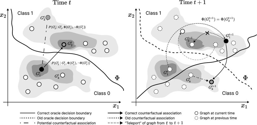
Figure 1: Counterfactuality under distributional drifts. (left) Given the decision boundary of the oracle $\Phi$ trained on the data at time $t$, graph $G_{2}^{t}$ is correctly associated as the counterfactual of $G_{1}^{t}$ since it satisfies Eq. 3. (right) Drift happens and $G^{t}_{1}$ is "teleported" at $G_{1}^{t+1}$ crossing the old (dotted red line) decision boundary. Here, $G_{2}^{t+1}$ cannot be a counterfactual for $G_{1}^{t+1}$ since $\Phi\left(G_{1}^{t+1}\right)=\Phi\left(G_{2}^{t+1}\right)$. Assuming that $G_{k}^{t+1}$ satisfies Eq. 3 at time $t+1$, we can signal a drift and potentially update $\Phi$’s decision boundary (green full line), thus changing the counterfactuals where applicable.

4 Methodology

Here, we describe our method, Dynamic GRAph Counterfactual Explainer, namely DyGRACE . DyGRACE is a semi-supervised GCE method that uses $\Phi$ in the first time step $t_{0}$ to obtain knowledge about the data distribution and search for valid counterfactuals while avoiding getting hints from its (possibly) outdated decision function for $t_{i}>t_{0}\;\forall i\in\left[1,T\right]$. To favour readability, we omit the time superscript from the formulas unless necessary for disambiguation.

Recall that we are in a binary classification scenario. However, the following observations can be easily extended to a multi-class classification problem. Here, we rely on two graph autoencoder s (GAE s) Kipf and Welling (2016), i.e., $f_{y},f_{\neg y}:\mathcal{G}\rightarrow\mathcal{G}$ that are responsible for learning how to represent each class in $Y$, respectively. At each time step, $G_{i}\in\mathcal{G}$ gets directed through one of the autoencoders based on $y=\Phi\left(G_{i}\right)$. The objective of each autoencoder during the training phase is to minimise the reconstruction error between the original graph $G_{i}$ and its learned representation $\hat{G}_{i}$. Generally, the reconstruction score is a function $h:\mathcal{G}\times\mathcal{G}\rightarrow\mathbb{R}$. For a pair of instances $\left(G_{i},G_{j}\right)$ s.t. $\Phi\left(G_{i}\right)\neq\Phi\left(G_{j}\right)$, we expect $h(G_{j},f_{y}\left(G_{j}\right))\geq h(G_{j},f_{\neg y}\left(G_{j}\right))$. This is the case since the autoencoder corresponding to the counterfactual class should know how to represent $G_{j}$, thus having a low reconstruction error. Contrarily, the autoencoder corresponding to the factual class should not be able to (at least not easily) reconstruct a counterfactual.

Once $f_{y}$ and $f_{\neg y}$ are trained, DyGRACE maximises the probability in Eq. 3 to find counterfactuals for all $G_{i}\in\mathcal{G}$. We model $P_{cf}$ by the parametric density function in Eq. 4 where $\alpha$, $\beta$, and $\gamma$ are learned weights.

$$\begin{gathered}\underset{G_{j}\in\mathcal{G}}{\arg\max}\;P_{cf}\left(G_{j}\;\middle|\;G_{i},\Phi\left(G_{i}\right),\neg\Phi\left(G_{i}\right)\right)\\ =\underset{G_{j}\in\mathcal{G}}{\arg\max}\left(\alpha h(G_{j},f_{y}\left(G_{j}\right))-\beta h(G_{j},f_{\neg y}\left(G_{j}\right))+\gamma g\left(G_{i},G_{j}\right)\right)\end{gathered}$$ (4)

where $y=\Phi\left(G_{i}\right)$, $g:\mathcal{G}\times\mathcal{G}\rightarrow\mathbb{R}$ measures the similarity between two graphs, and $\alpha$, $\beta$, and $\gamma$ are learned weights. Eq. 4 maximises the reconstruction error of $G_{j}$ from the factual autoencoder, minimise - hence the negation - the error of $G_{j}$ from the counterfactual autoencoder, and maximises the similarity of $G_{j}$ w.r.t. $G_{i}$. In other words, we search for counterfactuals that are far away from other factual graphs besides $G_{i}$.

Notice that the weights $\alpha$, $\beta$, and $\gamma$ in Eq. 4 can be solved via a logistic regression trained on a set of graph pairs. We assign pairs of graphs with $\left(G_{i},G_{j}\right)$ a label of $1$ if $\Phi\left(G_{j}\right)\neq\Phi\left(G_{i}\right)$, and $0$ otherwise. By solving this objective function, we can interpret the learned weights and assess the contribution of each component in the equation of finding the counterfactuals for each $G_{i}$. At inference time, we get a never-seen before graph $G^{*}$, and for all $G_{i}\in\mathcal{G}$, we calculate the reconstruction errors $h(G_{i},f_{0}\left(G_{i}\right))$ and $h(G_{i},f_{1}\left(G_{i}\right))$, and the similarity $g\left(G^{*},G_{i}\right)$. We use these values as input to the trained logistic regressor to find the “best” counterfactual candidate for $G^{*}$.

In the next iterations, we do not rely on $\Phi$’s predictions since they might not represent the reality of the new incoming data (see Fig. 1). Instead, we exploit the learned representation of the two GAE s from the previous iteration. In other words, for each $G_{i}^{t}\in\mathcal{G}$ s.t. $t\in[1,T]$, we exploit the reconstruction errors $h(G_{i}^{t},f_{0}(G_{i}^{t}))$ and $h(G_{i}^{t},f_{1}(G_{i}^{t}))$ to find the label of $G_{i}^{t}$. Notice that one of the GAE s embodies the latent representation of $G_{i}^{t}$, thus producing a smaller reconstruction error and playing the role of the factual autoencoder. Now, we can use the logistic regressor trained in at time $t-1$ to return the counterfactual $G_{j}^{t}\in\mathcal{G}$.

In practice, to support a continual adaptation of the learned graph representation of the GAE s, we find the top $k$ counterfactuals via the logistic regressor. We use these instances to update the knowledge of the counterfactual GAE and minimise the reconstruction error. Contrarily, we can use the same counterfactual candidates to maximise their reconstruction error by the factual GAE, thus steering it away from the counterfactual representation space. This goes in hand with the intuition of contrastive learning since the factual GAE, at each iteration, learns to be specific about the factual instances and is drawn away from potential counterfactuals. The same reasoning applies to the counterfactual GAE. After each iteration, the logistic regressor can be updated (or even trained from scratch) on the “newly gained” knowledge of the GAE s. In this way, the prediction decision function gets mimicked by the autoencoders instead of an external (possibly) black-box oracle $\Phi$.

Recall that we do not rely on the oracle $\Phi$ predictions in successive iterations but on the learned representation of the GAE s at previous ones. Nevertheless, DyGRACE can play the role of a drift detector based on the reconstruction errors at iteration $t$ and those at $t-1$. In other words, $f_{y}$ and $f_{\neg y}$ can be used to measure the reconstruction errors for $G_{i}^{t-1}\in\mathcal{G}$ based on $y=\Phi\left(G_{i}^{t-1}\right)$. Then, we can do the same for $G_{i}^{t}\in\mathcal{G}$ based on $y=\Phi\left(G_{i}^{t}\right)$. If the distributions of the reconstruction errors at $t$ and $t-1$ are different according to a statistic test (e.g., Kolmogorov-Smirnov test), then we can signal a distributional drift and update $\Phi$ accordingly. Afterwards, $f_{y}$ and $f_{\neg y}$ are retrained according to the updated $\Phi$, and Eq. 4 is optimised. However, notice that this procedure is supervised and depends on $\Phi$, which does not guarantee satisfactory performances at each iteration to guide the search for valid counterfactuals. Exploiting the learned representation of the GAE s in a semi-supervised manner as described above is more efficient and decouples itself from the underlying oracle $\Phi$.

5 DyGRACE’s performance analysis

Here, we assess the performances of DyGRACE and the other SoTA methods. First, we describe the adopted benchmarking datasets providing the details on their generation process (see Sec. 5.1). Then, we describe the evaluation metrics and the hyperparameters used to run each method (see Sec. 5.2). Finally, in Sec. 5.3, we provide a discussion of the performance of DyGRACE.

5.1 Benchmarking Datasets

Table 1: The dataset characteristics. $|\mathcal{G}|$ is the number of instances; $\mu(|V|)$ and $\sigma(|V|)$ represent the mean and std of the number of vertices per instance; $\mu(|E|)$ and $\sigma(|E|)$ represent the mean and std of the number of edges per instance; $|C_{i}|$ is the number of instances in class $i\in\{0,1\}$. $|T|$ represents the number of snapshots.

	$|T|$	$|\mathcal{G}|$		$\mu(|V|)\pm\sigma(|V|)$		$\mu(|E|)\pm\sigma(|E|)$		$|C_{0}|$		$|C_{1}|$
DynTree-Cycles	4	100		28 $\pm$ 0.00		27.62 $\pm$ 0.645		45.75		54.25
DBLP-Coauthors	10	36		13 $\pm$ 0.00		41.26 $\pm$ 6.69		27.27		8.73

We test DyGRACE on a synthetic dataset, namely Tree-Cycles, generated according to Prado-Romero and Stilo (2022); Ying et al. (2019), and a real dataset, namely DBLP-Coauthors Benson et al. (2018). See Table 1 for the dataset characteristics averaged over the different time snapshots.

Tree-Cycles Ying et al. (2019) contains cyclic (1) and acyclic (0) graphs. We extend this dataset by introducing the time dimension, allowing graphs to evolve while maintaining class membership. We repeat the dataset generation in Prado-Romero et al. (2022) at each time step. In this way, a particular graph $G_{i}^{t}$ can change its structure in $t+1$ and remain in the same class or move to the opposite one. This emulates a synthetic process of tracing the evolution of the graphs in the dataset according to time. Here, we guarantee that the number of instances per snapshot is the same.

The DBLP-Coauthors dataset comprises graphs representing authors, where edges denote co-authorship relationships, and edge weights signify the number of collaborations in a given year. We focus on the time frame [2000, 2010] and consider ego-networks of authors with at least ten collaborations in 2000. From this set, we randomly sample 1% due to the dataset’s scale. To trace the ego-network evolution from 2000 to 2010, we propagate ego-networks from the previous year whenever an author has no collaborations in a specific year $t$. Ego-networks are labelled 1 if their mean sum of edge weights is in the 75th percentile of average collaborations for a particular year $t$, otherwise labelled as 0.

5.2 Evaluation metrics and hyperparameter choice

We follow the suggestion in Prado-Romero et al. (2022) to evaluate each method and use multiple metrics to show a complete and fair assessment. To this end, we exploit Runtime, Oracle calls Abrate and Bonchi (2021), Correctness Guidotti (2022); Prado-Romero and Stilo (2022), Sparsity Prado-Romero and Stilo (2022); Yuan et al. (2023), and Graph Edit Distance Prado-Romero et al. (2022) as evaluation metrics. Since we return a list of counterfactuals for each input graph, we evaluate DyGRACE by reporting values of the previous metrics $@1,\dots,@k$.

Notice that DyGRACE is a flexible framework which can take any encoder-decoder combination to learn meaningful graph representations. Here, we rely on a 2-layer GCN encoder interleaved with ReLU activation functions. The output dimension of each convolution operation is 8. The decoder is a simple inner product between the learned graph representation $z$, as in Kipf and Welling (2016). We train each GAE for 50 and 150 epochs, respectively, for DTC and DBLP, and use the Adam optimiser with a learning rate of $10^{-3}$ and $10^{-4}$. We rely on L2 regularisation for the logistic regressor and use the default parameters of the scikit-learn package. We implement DyGRACE based on the GRETEL framework Prado-Romero et al. (2023); Prado-Romero and Stilo (2022). We did not perform any hyperparameter optimisation for DyGRACE.

5.3 Discussion

Table 2 depicts the performance of DyGRACE. We report averages on 10-fold cross-validation. We reserve $10\%$ of the first snapshot as test data and adapt the GAEs and the logistic regressor in an online fashion for the other snapshots. As a preliminary assessment of the performances of DyGRACE, we employ omniscient oracles for both datasets such that the correctness refers to the accuracy of the explainer w.r.t. the ground truth. Excluding the oracles’ performances allows the reader to understand each explainer’s limitations and benefits better. Where applicable, we report metrics $@1$ and $@k=10$. As anticipated in Sec. 4, DyGRACE accesses the oracle only in the first snapshot while relying on the GAE s in the successive snapshots.

In both datasets, DyGRACE has satisfactory results regarding correctness $@k$. Notice, however, that DBLP, being a real-world scenario, is far more complex than DTC. In DBLP, the ego networks belonging to the two classes share a similar structure, with the sole difference in the edge weights. Therefore, the correctness $@1$ in this scenario fluctuates (i.e., increasing until $t_{3}$, $t_{6}$, and decreasing afterwards). We believe this happens due to similar latent spaces that the two GAEs learn, which cannot completely distinguish between factual and counterfactual graphs.

It is interesting to notice that the correctness $@k$ has a non-decreasing trend for DTC, meaning that valid counterfactuals might not be the most probable w.r.t. the input graph. However, they get captured by the underlying logistic regressor. Meanwhile, in DBLP, the correctness $@1$ and $@k$ degrades after iteration $t_{7}$, meaning that the structure of the graphs mutates heavily, making the two GAEs unable to correctly represent the two classes. The GED follows a similar trend throughout the iterations, indicating that the logistic regressor does not need to go far away from the separating hyperplane to fetch valid counterfactuals. Additionally, this phenomenon suggests that the logistic regressor "pays attention" to the first two components of Eq. 4 to produce counterfactuals rather than concentrating more on the similarity of the instance with its potential counterfactual.

One drawback that could hinder DyGRACE’s usability is the running time, especially in successive iterations (see DBLP) where there are distributional shifts and the two GAEs need to update. However, one could implement an update trigger mechanism only in those scenarios where substantial drifts happen, which can get signalled according to a statistical test w.r.t. the reconstruction errors of the current and previous iterations (see Sec. 4).

Table 2: Average of DyGRACE’s performance on DynTree-Cycles (DTC) and DBLP-Coauthors (DBLP) on 10-fold cross-validation.

				Runtime (s) $\downarrow$		Correctness $\uparrow$				Sparsity $\downarrow$				GED $\downarrow$					Oracle Calls $\downarrow$
						@1		@k		@1		@k		@1		@k
DTC		$t_{0}$		$24.73^{\pm 70.419}$		$0.40^{\pm 0.490}$		$1.00^{\pm 0.000}$		$0.65^{\pm 0.109}$		$0.72^{\pm 0.114}$		$36.90^{\pm 5.839}$		$40.04^{\pm 6.272}$			$9000.00^{\pm 0.00}$
		$t_{1}$		$73.35^{\pm 3.622}$		$0.60^{\pm 0.490}$		$1.00^{\pm 0.000}$		$0.69^{\pm 0.087}$		$0.73^{\pm 0.085}$		$38.60^{\pm 4.652}$		$40.46^{\pm 4.725}$			$0.00^{\pm 0.00}$
		$t_{2}$		$74.62^{\pm 6.225}$		$0.70^{\pm 0.458}$		$1.00^{\pm 0.000}$		$0.73^{\pm 0.038}$		$0.75^{\pm 0.079}$		$40.50^{\pm 2.291}$		$41.68^{\pm 4.366}$			$0.00^{\pm 0.00}$
		$t_{3}$		$65.99^{\pm 8.409}$		$0.40^{\pm 0.490}$		$1.00^{\pm 0.000}$		$0.76^{\pm 0.065}$		$0.74^{\pm 0.090}$		$42.50^{\pm 3.775}$		$41.16^{\pm 4.983}$			$0.00^{\pm 0.00}$
DBLP		$t_{0}$		$12.83^{\pm 32.599}$		$0.38^{\pm 0.484}$		$1.00^{\pm 0.000}$		$0.67^{\pm 0.186}$		$0.71^{\pm 0.194}$		$28.50^{\pm 8.617}$		$30.04^{\pm 9.499}$			$9900.00^{\pm 0.00}$
		$t_{1}$		$140.21^{\pm 53.821}$		$0.25^{\pm 0.433}$		$0.88^{\pm 0.331}$		$0.54^{\pm 0.315}$		$0.62^{\pm 0.238}$		$35.25^{\pm 47.872}$		$40.24^{\pm 48.264}$			$0.000^{\pm 0.00}$
		$t_{2}$		$121.29^{\pm 57.151}$		$0.12^{\pm 0.331}$		$0.88^{\pm 0.331}$		$1.52^{\pm 2.709}$		$3.59^{\pm 6.178}$		$18.88^{\pm 15.070}$		$34.82^{\pm 33.389}$			$0.000^{\pm 0.00}$
		$t_{3}$		$150.73^{\pm 20.020}$		$0.38^{\pm 0.484}$		$0.88^{\pm 0.331}$		$0.85^{\pm 0.489}$		$0.81^{\pm 0.384}$		$63.12^{\pm 51.033}$		$57.86^{\pm 44.450}$			$0.000^{\pm 0.00}$
		$t_{4}$		$161.89^{\pm 10.609}$		$0.25^{\pm 0.433}$		$0.62^{\pm 0.484}$		$0.63^{\pm 0.261}$		$0.58^{\pm 0.263}$		$21.62^{\pm 15.337}$		$20.51^{\pm 15.186}$			$0.000^{\pm 0.00}$
		$t_{5}$		$162.77^{\pm 13.782}$		$0.50^{\pm 0.500}$		$1.00^{\pm 0.000}$		$1.01^{\pm 1.388}$		$0.75^{\pm 0.835}$		$21.12^{\pm 10.361}$		$21.71^{\pm 12.553}$			$0.000^{\pm 0.00}$
		$t_{6}$		$165.39^{\pm 15.160}$		$0.50^{\pm 0.500}$		$1.00^{\pm 0.000}$		$2.26^{\pm 3.125}$		$2.21^{\pm 4.238}$		$55.00^{\pm 39.528}$		$53.36^{\pm 42.852}$			$0.000^{\pm 0.00}$
		$t_{7}$		$81.22^{\pm 82.797}$		$0.12^{\pm 0.331}$		$0.50^{\pm 0.500}$		$1.44^{\pm 3.244}$		$3.13^{\pm 5.679}$		$11.62^{\pm 19.118}$		$23.80^{\pm 32.100}$			$0.000^{\pm 0.00}$
		$t_{8}$		$76.85^{\pm 75.487}$		$0.12^{\pm 0.331}$		$0.50^{\pm 0.500}$		$0.45^{\pm 0.535}$		$0.84^{\pm 0.671}$		$17.88^{\pm 23.861}$		$33.32^{\pm 24.627}$			$0.000^{\pm 0.00}$
		$t_{9}$		$66.97^{\pm 67.959}$		$0.25^{\pm 0.433}$		$0.50^{\pm 0.500}$		$0.44^{\pm 0.450}$		$0.67^{\pm 0.257}$		$33.75^{\pm 34.387}$		$51.85^{\pm 20.576}$			$0.000^{\pm 0.00}$
		$t_{10}$		$63.07^{\pm 65.097}$		$0.25^{\pm 0.433}$		$0.38^{\pm 0.484}$		$0.90^{\pm 1.310}$		$0.97^{\pm 0.685}$		$57.62^{\pm 69.611}$		$77.09^{\pm 62.334}$			$0.000^{\pm 0.00}$

6 Conclusion

We demonstrated the effectiveness of our semi-supervised Graph Counterfactual Explainer across synthetic and real-world datasets. Deployed on the synthetic Tree-Cycles dataset and the real-world DBLP-Coauthors dataset, DyGRACE showcased satisfactory results in terms of correctness. Despite the complexity of the DBLP dataset due to its real-world nature, DyGRACE managed to discern between factual and counterfactual graphs to a large extent.

The continual trend of increasing correctness in both datasets asserts DyGRACE’s ability to capture valid counterfactuals, even when they may not be the most probable concerning the input graph. This is particularly impressive given that GED remained stable throughout iterations, indicating that the model doesn’t have to deviate significantly from the separating hyperplane to identify valid counterfactuals. Nonetheless, DyGRACE’s potential downside lies in its extensive runtime during consecutive iterations, particularly visible in datasets with significant distributional shifts. We suggest implementing an update trigger mechanism that activates only when substantial drifts occur to alleviate this issue. This approach would rely on a statistical test concerning the reconstruction errors of current and previous iterations.

Our findings support DyGRACE as a promising, flexible framework that can learn meaningful graph representations for counterfactual explanations. Thus, DyGRACE offers exciting new opportunities for future research.

References

- Pawelczyk et al. [2023] Martin Pawelczyk, Tobias Leemann, Asia Biega, and Gjergji Kasneci. On the trade-off between actionable explanations and the right to be forgotten. In Proceedings of the Eleventh International Conference on Learning Representations, 2023.
- Bashir et al. [2017] Sulaimon Adebayo Bashir, Andrei Petrovski, and Daniel Doolan. A framework for unsupervised change detection in activity recognition. International journal of pervasive computing and communications, 13(2):157–175, 2017.
- Haug and Kasneci [2021] Johannes Haug and Gjergji Kasneci. Learning parameter distributions to detect concept drift in data streams. In 2020 25th International Conference on Pattern Recognition (ICPR), pages 9452–9459. IEEE, 2021.
- Lughofer et al. [2016] Edwin Lughofer, Eva Weigl, Wolfgang Heidl, Christian Eitzinger, and Thomas Radauer. Recognizing input space and target concept drifts in data streams with scarcely labeled and unlabelled instances. Information Sciences, 355:127–151, 2016.
- Sethi and Kantardzic [2017] Tegjyot Singh Sethi and Mehmed Kantardzic. On the reliable detection of concept drift from streaming unlabeled data. Expert Systems with Applications, 82:77–99, 2017.
- Dumitrescu et al. [2022] Bogdan Dumitrescu, Andra Băltoiu, and Stefania Budulan. Anomaly detection in graphs of bank transactions for anti money laundering applications. IEEE Access, 10:47699–47714, 2022. doi:10.1109/ACCESS.2022.3170467.
- Madeddu et al. [2020] Lorenzo Madeddu, Giovanni Stilo, and Paola Velardi. A feature-learning-based method for the disease-gene prediction problem. International Journal of Data Mining and Bioinformatics, 24(1):16–37, 2020.
- Wu et al. [2022] Xixi Wu, Yun Xiong, Yao Zhang, Yizhu Jiao, Caihua Shan, Yiheng Sun, Yangyong Zhu, and Philip S Yu. Clare: A semi-supervised community detection algorithm. In Proceedings of the 28th ACM SIGKDD Conference on Knowledge Discovery and Data Mining, pages 2059–2069, 2022.
- Prado-Romero et al. [2022] Mario Alfonso Prado-Romero, Bardh Prenkaj, Giovanni Stilo, and Fosca Giannotti. A survey on graph counterfactual explanations: Definitions, methods, evaluation. arXiv preprint arXiv:2210.12089, 2022.
- Faber et al. [2020] Lukas Faber, Amin K Moghaddam, and Roger Wattenhofer. Contrastive graph neural network explanation. In Proceedings of the 37th Graph Representation Learning and Beyond Workshop at ICML 2020, page 28. International Conference on Machine Learning, 2020.
- Abrate and Bonchi [2021] Carlo Abrate and Francesco Bonchi. Counterfactual graphs for explainable classification of brain networks. In Proceedings of the 27th ACM SIGKDD Conference on Knowledge Discovery & Data Mining, pages 2495–2504, 2021.
- Bajaj et al. [2021] Mohit Bajaj, Lingyang Chu, Zi Yu Xue, Jian Pei, Lanjun Wang, Peter Cho-Ho Lam, and Yong Zhang. Robust counterfactual explanations on graph neural networks. Advances in Neural Information Processing Systems, 34:5644–5655, 2021.
- Huang et al. [2023] Zexi Huang, Mert Kosan, Sourav Medya, Sayan Ranu, and Ambuj Singh. Global counterfactual explainer for graph neural networks. In Proceedings of the Sixteenth ACM International Conference on Web Search and Data Mining, pages 141–149, 2023.
- Liu et al. [2021] Yifei Liu, Chao Chen, Yazheng Liu, Xi Zhang, and Sihong Xie. Multi-objective explanations of gnn predictions. In 2021 IEEE International Conference on Data Mining (ICDM), pages 409–418. IEEE, 2021.
- Wellawatte et al. [2022] Geemi P Wellawatte, Aditi Seshadri, and Andrew D White. Model agnostic generation of counterfactual explanations for molecules. Chemical science, 13(13):3697–3705, 2022.
- Cai et al. [2022] Ruichu Cai, Yuxuan Zhu, Xuexin Chen, Yuan Fang, Min Wu, Jie Qiao, and Zhifeng Hao. On the probability of necessity and sufficiency of explaining graph neural networks: A lower bound optimization approach. arXiv preprint arXiv:2212.07056, 2022.
- Lucic et al. [2022] Ana Lucic, Maartje A Ter Hoeve, Gabriele Tolomei, Maarten De Rijke, and Fabrizio Silvestri. Cf-gnnexplainer: Counterfactual explanations for graph neural networks. In International Conference on Artificial Intelligence and Statistics, pages 4499–4511. PMLR, 2022.
- Tan et al. [2022] Juntao Tan, Shijie Geng, Zuohui Fu, Yingqiang Ge, Shuyuan Xu, Yunqi Li, and Yongfeng Zhang. Learning and evaluating graph neural network explanations based on counterfactual and factual reasoning. In Proceedings of the ACM Web Conference 2022, WWW ’22, page 1018–1027, New York, NY, USA, 2022. Association for Computing Machinery. ISBN 9781450390965. URL https://doi.org/10.1145/3485447.3511948.
- Wu et al. [2021] Haoran Wu, Wei Chen, Shuang Xu, and Bo Xu. Counterfactual supporting facts extraction for explainable medical record based diagnosis with graph network. In Proceedings of the 2021 Conference of the North American Chapter of the Association for Computational Linguistics: Human Language Technologies, pages 1942–1955, 2021.
- Nguyen et al. [2023] T. Nguyen, T. P. Quinn, T. Nguyen, and T. Tran. Explaining black box drug target prediction through model agnostic counterfactual samples. IEEE/ACM Transactions on Computational Biology and Bioinformatics, 20(02):1020–1029, mar 2023. ISSN 1557-9964. doi:10.1109/TCBB.2022.3190266.
- Numeroso and Bacciu [2021] Danilo Numeroso and Davide Bacciu. Meg: Generating molecular counterfactual explanations for deep graph networks. In 2021 International Joint Conference on Neural Networks (IJCNN), pages 1–8. IEEE, 2021.
- Ma et al. [2022] Jing Ma, Ruocheng Guo, Saumitra Mishra, Aidong Zhang, and Jundong Li. CLEAR: generative counterfactual explanations on graphs. In NeurIPS, 2022. URL http://papers.nips.cc/paper_files/paper/2022/hash/a69d7f3a1340d55c720e572742439eaf-Abstract-Conference.html.
- Sun et al. [2021] Yi Sun, Abel Valente, Sijia Liu, and Dakuo Wang. Preserve, promote, or attack? gnn explanation via topology perturbation. arXiv preprint arXiv:2103.13944, 2021.
- Livi and Rizzi [2013] Lorenzo Livi and Antonello Rizzi. The graph matching problem. Pattern Analysis and Applications, 16:253–283, 2013.
- Prado-Romero et al. [2023] Mario Alfonso Prado-Romero, Bardh Prenkaj, and Giovanni Stilo. Revisiting countergan for counterfactual explainability of graphs. In Krystal Maughan, Rosanne Liu, and Thomas F. Burns, editors, The First Tiny Papers Track at ICLR 2023, Tiny Papers @ ICLR 2023, Kigali, Rwanda, May 5, 2023. OpenReview.net, 2023. URL https://openreview.net/pdf?id=d0m0Rl15q3g.
- Nemirovsky et al. [2022] Daniel Nemirovsky, Nicolas Thiebaut, Ye Xu, and Abhishek Gupta. Countergan: Generating counterfactuals for real-time recourse and interpretability using residual gans. In James Cussens and Kun Zhang, editors, Uncertainty in Artificial Intelligence, Proceedings of the Thirty-Eighth Conference on Uncertainty in Artificial Intelligence, UAI 2022, 1-5 August 2022, Eindhoven, The Netherlands, volume 180 of Proceedings of Machine Learning Research, pages 1488–1497. PMLR, 2022. URL https://proceedings.mlr.press/v180/nemirovsky22a.html.
- Kipf and Welling [2016] Thomas N Kipf and Max Welling. Variational graph auto-encoders. In NeurIPS Workshop on Bayesian Deep Learning, 2016.
- Prado-Romero and Stilo [2022] Mario Alfonso Prado-Romero and Giovanni Stilo. Gretel: Graph counterfactual explanation evaluation framework. In Proceedings of the 31st ACM International Conference on Information & Knowledge Management, pages 4389–4393, 2022.
- Ying et al. [2019] Zhitao Ying, Dylan Bourgeois, Jiaxuan You, Marinka Zitnik, and Jure Leskovec. Gnnexplainer: Generating explanations for graph neural networks. In Hanna M. Wallach, Hugo Larochelle, Alina Beygelzimer, Florence d’Alché-Buc, Emily B. Fox, and Roman Garnett, editors, Advances in Neural Information Processing Systems 32: Annual Conference on Neural Information Processing Systems 2019, NeurIPS 2019, December 8-14, 2019, Vancouver, BC, Canada, pages 9240–9251, 2019. URL https://proceedings.neurips.cc/paper/2019/hash/d80b7040b773199015de6d3b4293c8ff-Abstract.html.
- Benson et al. [2018] Austin R Benson, Rediet Abebe, Michael T Schaub, Ali Jadbabaie, and Jon Kleinberg. Simplicial closure and higher-order link prediction. Proceedings of the National Academy of Sciences, 115(48):E11221–E11230, 2018.
- Guidotti [2022] R. Guidotti. Counterfactual explanations and how to find them: literature review and benchmarking. Data Mining and Knowledge Discovery, pages 1–55, 2022.
- Yuan et al. [2023] Hao Yuan, Haiyang Yu, Shurui Gui, and Shuiwang Ji. Explainability in graph neural networks: A taxonomic survey. IEEE Transactions Pattern Analaysis and Machine Intelligence, 45(5):5782–5799, 2023. doi:10.1109/TPAMI.2022.3204236. URL https://doi.org/10.1109/TPAMI.2022.3204236.
- Prado-Romero et al. [2023] Mario Alfonso Prado-Romero, Bardh Prenkaj, and Giovanni Stilo. Developing and evaluating graph counterfactual explanation with gretel. In Proceedings of the Sixteenth ACM International Conference on Web Search and Data Mining, pages 1180–1183, 2023.