A Quantize-then-Estimate Protocol for CSI Acquisition in IRS-Aided Downlink Communication

Abstract

For intelligent reflecting surface (IRS) aided downlink communication in frequency division duplex (FDD) systems, the overhead for the base station (BS) to acquire channel state information (CSI) is extremely high under the conventional “estimate-then-quantize” scheme, where the users first estimate and then feed back their channels to the BS. Recently, [1] revealed a strong correlation in different users’ cascaded channels stemming from their common BS-IRS channel component, and leveraged such a correlation to significantly reduce the pilot transmission overhead in IRS-aided uplink communication. In this paper, we aim to exploit the above channel property for reducing the overhead of both pilot transmission and feedback transmission in IRS-aided downlink communication. Different from the uplink counterpart where the BS possesses the pilot signals containing the CSI of all the users, in downlink communication, the distributed users merely receive the pilot signals containing their own CSI and cannot leverage the correlation in different users’ channels revealed in [1]. To tackle this challenge, this paper proposes a novel “quantize-then-estimate” protocol in FDD IRS-aided downlink communication. Specifically, the users first quantize their received pilot signals, instead of the channels estimated from the pilot signals, and then transmit the quantization bits to the BS. After de-quantizing the pilot signals received by all the users, the BS estimates all the cascaded channels by leveraging the correlation embedded in them, similar to the uplink scenario. Under this protocol, we propose efficient methods for quantization at the user side and channel estimation at the BS side. Furthermore, we manage to show both analytically and numerically the great overhead reduction in terms of pilot transmission and feedback transmission arising from our proposed “quantize-then-estimate” protocol.

I Introduction

Channel state information (CSI) acquisition is of paramount importance to fully reap the beamforming gain promised by intelligent reflecting surface (IRS). However, such a task is challenging due to the vast number of channel coefficients associated with the IRS. This paper considers IRS-assisted downlink communication in a frequency division duplex (FDD) system, where a multi-antenna base station (BS) needs to know the BS-IRS-user cascaded channels of all the users for designing its own and the IRS’s beamforming vectors. Note that CSI acquisition in IRS-aided downlink communication is essentially a distributed source coding (DSC) problem [2], where the core question is what information should be fed back by the users after they receive the pilot signals from the BS, such that the BS can acquire the CSI with the shortest pilot signals transmitted in the downlink and the minimum quantization bits transmitted in the uplink.

In [3, 4], the “estimate-then-quantize” protocol [5, 6, 7] was utilized to solve the above DSC problem, where each user first estimates its BS-IRS-user cascaded channels based on its received pilot signals, and then feeds back the quantized channels to the BS. Specifically, [3] utilizes the sparsity in the IRS-BS channel to reduce the dimension of the channels for feedback. Moreover, [4] focused on the feedback of the channel gains and proposed a novel cascaded codebook that is synthesized by two sub-codebooks whose codewords are cascaded by line-of-sight and non-line-of-sight components.

Merely focusing on reducing the feedback overhead, the above works did not consider how to reduce the overhead in the pilot transmission phase, which is also huge in IRS-aided communication. Moreover, the “estimate-then-quantize” protocol adopted in these works performs well for conventional downlink communication without IRSs, but is not theoretically optimal for IRS-aided downlink communication. The reason is as follows. Users’ channels are independent without IRSs, and according to DSC theory, estimating the independent channels in a distributed manner at the user side will not cause information loss. However, [1] revealed a strong correlation among different users’ cascaded channels in IRS-aided systems, which arises from the common BS-IRS channel to all the users. With this correlation, the classic DSC theory implies that each user should not independently estimate its cascaded channels.

To take advantage of the above channel correlation for reducing CSI acquisition overhead in both the pilot transmission phase and the feedback transmission phase, even if the users are distributed and cannot cooperate with each other, this paper proposes a novel “quantize-then-estimate” protocol in FDD IRS-aided downlink communication. In sharp contrast to the “estimate-then-quantize” counterpart, our strategy makes each user first quantize its received pilot signals and then feed back the quantized pilots to the BS. After de-quantization, the BS knows the pilot signals received by all the users, which contain the global CSI. Therefore, the BS can exploit the channel correlation revealed in [1] to efficiently estimate the cascaded channels of all the users. The benefits of the proposed protocol for overhead reduction are two-fold. First, the BS is able to estimate the channels based on shorter pilot signals as shown in [1], i.e., the number of time slots for BS’s pilot transmission can be reduced. Second, because each user receives fewer pilot symbols, the number of quantization bits for feedback transmission is also reduced. In this paper, we will analytically and numerically verify the above overhead reduction for CSI acquisition in IRS-aided systems.

II System Model

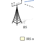
Figure 1: An IRS-aided downlink communication system.

We study the downlink communication in an FDD system which consists of a BS with $M$ antennas, $K$ single-antenna users, and an IRS with $N$ passive reflecting elements, as shown in Fig. 1. However, the overhead to acquire CSI in IRS-assisted communication systems is high due to the large number of IRS elements $N$. To tackle this challenge, we adopt an IRS element grouping strategy as in [8, 9]. Specifically, the IRS elements are divided into $D$ sub-surfaces to reduce the number of channels to be estimated, and the IRS elements within each sub-surface share a common reflection coefficient. Let ${\phi}_{d,i}=\nu_{d,i}e^{j\theta_{d,i}}\in\mathbb{C}$ denote the reflection coefficient of the $d$-th IRS sub-surface at time slot $i$, where $\nu_{d,i}\in[0,1]$ and $\theta_{d,i}\in[0,2\pi)$ denote the amplitude and the phase shift of $\phi_{d,i}$, respectively.

We assume a quasi-static block fading channel model, where the channels remain approximately constant in each coherence block. In addition, as shown in Fig. 1, we assume that the direct channels between the BS and users are blocked, and the signals can only be transmitted through the IRS reflecting channels to the users. The baseband equivalent channels from the BS to the $d$-th IRS sub-surface, and from the $d$-th IRS sub-surface to user $k$ are denoted by ${\bm{r}}_{d}\in\mathbb{C}^{M\times 1}$ and ${t}_{k,d}\in\mathbb{C},k=1,\cdots,K,d=1,\cdots,D$, respectively. For convenience, define ${\bm{R}}=[{\bm{r}}_{1},\cdots,{\bm{r}}_{D}]$ as the overall channels from the BS to the IRS, and ${\bm{t}}_{k}=[{t}_{k,1},\cdots,{t}_{k,D}]^{T}$ as the channels from the IRS to user $k$. Moreover, the cascaded reflecting channels from the BS to user $k$ through the $d$-th IRS sub-surface is expressed as

$${\bm{g}}_{k,d}={t}_{k,d}{\bm{r}}_{d}\in\mathbb{C}^{M\times 1},~{}~{}\forall d,k.$$ (1)

In the downlink communication, the pilot symbols transmitted from the BS at time slot $i$ are denoted by ${\bm{x}}_{i}=[x_{i,1},\cdots,x_{i,M}]^{T}\in\mathbb{C}^{M\times 1},i=1,\cdots,T$, where $T$ is the number of time slots to transmit the pilots. Then, the received signal of user $k$ at time slot $i$ is expressed as

$$y_{k,i} =\sum_{d=1}^{D}{\phi}_{d,i}{\bm{g}}_{k,d}^{T}\sqrt{p}{\bm{x}}_{i}+z_{k,i},~{}~{}\forall k,i,$$ (2)

where $p$ denotes the transmit power at the BS, and $z_{k,i}\sim\mathcal{CN}(0,\sigma_{z}^{2})$ denotes the additive white Gaussian noise (AWGN) of user $k$ at time slot $i$.

III A Novel Quantize-then-Estimate Protocol

In this paper, we aim to propose a low-overhead channel estimation and feedback scheme such that the BS can efficiently acquire the cascaded channels ${\bm{g}}_{k,d}$’s, $\forall k,d$, to design the downlink beamforming vectors. In this section, we will first overview the conventional method for channel estimation and feedback in our considered IRS-assisted FDD systems, and show its disadvantages. Then, we will propose a novel strategy that can exploit the unique channel property in IRS-assisted communication to reduce the channel estimation and feedback overhead.

III-A Traditional Estimate-then-Quantize Scheme

Without IRS, channel estimation and feedback have been widely studied for downlink FDD systems [5, 6, 7]. In the IRS-assisted network, we may apply the following ”estimate-then-quantize” strategy for channel estimation and feedback.

• Phase I (Estimation): In the first phase, each user $k$ first receives the pilot signals from the BS as shown in (2) and then estimates its cascaded channel ${\bm{g}}_{k,d}$’s, $\forall d$, based on the existing method proposed in [8, 9, 10, 11].

• Phase II (Feedback): In the second phase, each user quantizes its estimated channels and feeds back the quantization bits to the BS. The BS de-quantizes the quantization bits to recover the cascaded channels of all the users.

Although the above estimate-then-quantize strategy works well in conventional systems without IRS, its performance is poor in our considered IRS-assisted systems. Specifically, under the above scheme, the minimum number of time slots for user $k$ to estimate ${\bm{g}}_{k,d}$’s, $d=1,\cdots,D$, in Phase I is $T_{min}=MD$ [1]. Moreover, each user $k$ needs to feed back $MD$ channel coefficients in ${\bm{g}}_{k,d}$’s, $d=1,\cdots,D$, to the BS in Phase II. Recently, it has been revealed in [1] that there is a lot of redundancy in users’ cascaded channels and the number of independent unknown variables in ${\bm{g}}_{k,d}$’s, $k=1,\cdots,K,d=1,\cdots,D$, is much smaller than $KMD$. Specifically, if we focus on a particular IRS sub-surface $d$, then the channel between the BS and the $d$-th sub-surface of the IRS, i.e., ${\bm{r}}_{d}$, is common among the cascaded channels ${\bm{g}}_{k,d}$’s of all the users. As a result, according to (1), we have

$${\bm{g}}_{k,d}=\lambda_{k,d}{\bm{g}}_{k_{d},d},~{}~{}\forall k\neq k_{d},~{}d=1,\cdots,D,$$ (3)

where $k_{d}$ is the index of the reference user selected for IRS sub-surface $d$, and the channel ratio between user $k$ and reference user $k_{d}$ is given by

$$\lambda_{k,d}=\frac{{t}_{k,d}}{{t}_{k_{d},d}}.$$ (4)

(3) and (4) indicate that for each IRS sub-surface $d$, if the cascaded channel of the reference user $k_{d}$, i.e., ${\bm{g}}_{k_{d},d}$, is known, a scalar $\lambda_{k,d}$ is sufficient for the BS to know the cascaded channel vector of user $k$, i.e., ${\bm{g}}_{k,d}$. In other words, the BS just needs to know $MD+(K-1)D$ channel coefficients in ${\bm{g}}_{k_{d},d}$’s, $d=1,\cdots,D$, and $\lambda_{k,d}$’s, $\forall k\neq k_{d}$, $d=1,\cdots,D$. Therefore, the number of time slots for pilot transmission in Phase I and the number of quantization bits in Phase II can be hugely reduced in IRS-assisted downlink communication, if the channel property shown in (3) and (4) can be properly utilized. However, the conventional estimate-then-quantize scheme does not take advantage of (3) and (4) for reducing the overhead.

III-B Proposed Quantize-then-Estimate Scheme

In this sub-section, we propose a novel strategy that can leverage (3) and (4) to significantly reduce the overhead for channel estimation and feedback in IRS-assisted downlink communication. Note that (3) and (4) reveal the correlation among different users’ cascaded channels, while the users are distributed and cannot cooperate with each other to leverage such correlation for channel estimation. To overcome this issue, we propose a quantize-then-estimate protocol as detailed below.

• Phase I (Feedback): In the first phase, all the users receive the pilot signals from the BS as shown in (2). However, instead of estimating its own channels, each user $k$ quantizes its received pilot signals over $T$ time slots, i.e., ${\bm{y}}_{k}=[y_{k,1},...,y_{k,T}]^{T}$, and feeds back the quantization bits to the BS.

• Phase II (Estimation): In the second phase, the BS de-quantizes the received quantization bits for recovering the pilot signals received by all the users. Then, with the above global information, the BS is able to leverage the correlation among different users’ channels shown in (3) and (4) to estimate ${\bm{g}}_{k,d}$’s more efficiently.

Note that the key difference between our proposed quantize-then-estimate scheme and the conventional estimate-then-quantize scheme shown in Section III-A lies in what is fed back from the users to the BS and who performs channel estimation. Under our scheme, users feed back their received pilot signals such that the BS can perform a joint estimation of different users’ channels by leveraging (3) and (4). The benefits of the above joint estimation are two-fold. First, as shown in [1], the minimum number of time slots for channel estimation, i.e., $T_{min}$, can be reduced from $MD$ to $D+\lceil(M-1)D/K\rceil$ by leveraging (3) and (4), where $\lceil\cdot\rceil$ denotes the ceiling function. Second, because signals from fewer time slots need to be quantized, the feedback overhead is significantly reduced. Specifically, without utilizing (3) and (4), all the users need to quantize $KMD$ symbols in ${\bm{g}}_{k,d}$’s; while under our proposed scheme, as will be shown later in Section IV, all the users only need to quantize $KD+K\lceil(M-1)D/K\rceil$ symbols in ${\bm{y}}_{k}$’s under the case of $K<D$, which is true in practical IRS-assisted systems.

In the following section, we will first introduce how to quantize ${\bm{y}}_{k}$’s by the users, and then introduce how to estimate the channels via leveraging (3) and (4) by the BS.

IV Quantization and Estimation Design

IV-A Quantization at User Side

In this sub-section, we introduce how the users quantize the received pilot signals. Specifically, the received pilot signal of each user $k$ at time slot $i$, i.e., $y_{k,i}$, $i=1,\cdots,T$, is quantized by a scalar quantization method. At time slot $i$, the codebook for quantizing user $k$’s received pilot, i.e., $y_{k,i}$, is denoted by $\mathcal{C}_{k,i}=\{{w}^{k,i}_{1},\cdots,{w}^{k,i}_{L}\}$, which consists of $L$ codewords. Based on the probability density function of $y_{k,i}$, the codebook can be designed via the Lloyd algorithm [12]. Given the codebook $\mathcal{C}_{k,i}$, the codeword index and the corresponding codeword to quantize $y_{k,i}$ are given by

$$l_{k,i}^{\ast}=\underset{l=1,\cdots,L}{\arg\min}~{}\mathcal{D}(y_{k,i},{w}^{k,i}_{l}),$$

$$\tilde{y}_{k,i}=w^{k,i}_{l^{\ast}_{k,i}},~{}~{}\forall k,i,$$ (5)

where $\mathcal{D}(y_{k,i},{w}^{k,i}_{l})=\|y_{k,i}-{w}^{k,i}_{l}\|^{2}_{2}$ denotes the distortion function between ${y}_{k,i}$ and the codeword ${w}^{k,i}_{l}$. Then, the quantized signal $\tilde{y}_{k,i}$ is modeled as [12]:

$$\tilde{y}_{k,i}=y_{k,i}+e_{k,i},~{}~{}\forall k,i,$$ (6)

where $e_{k,i}$ denotes the quantization noise. Last, at time slot $i$, user $k$ transmits its codeword index $l_{k,i}^{\ast}$ using $\lceil\log_{2}L\rceil$ quantization bits to the BS. It is assumed that the feedback channel is error-free such that the quantization bits can be perfectly received by the BS.

IV-B Channel Estimation at BS Side

In this sub-section, we introduce how the BS can estimate the channels. To begin with, the BS de-quantizes the quantization bits to recover the pilot signals received by all the users. Based on the codebooks $\mathcal{C}_{k,i}$’s, the BS can de-quantize user $k$’s received pilot signals over $T$ time slots as $\tilde{\bm{y}}_{k}=[\tilde{y}_{k,1},\cdots,\tilde{y}_{k,T}]^{T},k=1,\cdots,K$.

Subsequently, based on the above de-quantized signals, the BS adopts a two-step channel estimation method, where in the first step consisting of $\tau_{1}<T$ time slots, the BS estimates $\lambda_{k,d}$’s, $\forall k\neq k_{d}$ and $\forall d$, based on $\tilde{y}_{k,1},\cdots,\tilde{y}_{k,\tau_{1}}$, while in the second step consisting of $\tau_{2}=T-\tau_{1}$ time slots, the BS estimates ${\bm{g}}_{k_{d},d}$’s based on $\tilde{y}_{k,\tau_{1}+1},\cdots,\tilde{y}_{k,\tau_{1}+\tau_{2}}$, $\forall k,d$. Last, user $k$’s cascaded channels can be recovered based on (3), $\forall k$. In the following, we introduce how to estimate $\lambda_{k,d}$’s in Step 1 and ${\bm{g}}_{k_{d},d}$’s in Step 2.

Step 1 (Estimation of channel ratios $\lambda_{k,d}$’s): In the first step, the de-quantized received signals $\tilde{y}_{k,i}$’s given in (6) can be re-written as

$$\tilde{y}_{k,i}=\sum_{d=1}^{D}{\phi}_{d,i}\alpha_{k,d,i}+z_{k,i}+e_{k,i},~{}~{}\forall k,i=1,\cdots,\tau_{1},$$ (7)

where

$$\alpha_{k,d,i}=\begin{cases}$$\sqrt{p}{\bm{g}}_{k_{d},d}^{T}{\bm{x}}_{i}$$,&\mbox{if $k=k_{d}$},\\ $$\sqrt{p}{{\lambda}}_{k,d}{\bm{g}}_{k_{d},d}^{T}{\bm{x}}_{i}$$,&\mbox{if $k\neq k_{d}$},\end{cases}~{}~{}\forall d,i=1,\cdots,\tau_{1}.$$ (8)

Note that if we can perfectly recover $\alpha_{k,d,i}$’s in (8), then the channel ratio can be obtained by

$${\lambda}_{k,d}=\frac{\alpha_{k,d,i}}{\alpha_{k_{d},d,i}},~{}~{}\forall k\neq k_{d},\forall d,i=1,\cdots,\tau_{1}.$$ (9)

The main challenge to estimate $\alpha_{k,d,i}$’s in (8) is that for each $k$, the BS has to estimate $\tau_{1}D$ unknown variables, i.e., $\alpha_{k,d,i}$’s, $d=1,\cdots,D,i=1,\cdots,\tau_{1}$, using $\tau_{1}<\tau_{1}D$ observations, i.e., $\tilde{y}_{k,i}$’s, $i=1,\cdots,\tau_{1}$. To solve this challenge, we propose to set identical pilot signals over all time slots in Step 1, i.e.,

$${\bm{x}}_{i}={\bm{x}},~{}~{}i=1,\cdots,\tau_{1}.$$ (10)

In this case, the received signal in (7) reduces to

$$\tilde{y}_{k,i}=\sum_{d=1}^{D}{\phi}_{d,i}{\alpha}_{k,d}+z_{k,i}+e_{k,i},~{}~{}\forall k,i=1,\cdots,\tau_{1},$$ (11)

where

$${\alpha}_{k,d}=\begin{cases}$$\sqrt{p}{\bm{g}}_{k_{d},d}^{T}{\bm{x}}$$,&\mbox{if $k=k_{d}$},\\ $$\sqrt{p}{\lambda}_{k,d}{\bm{g}}_{k_{d},d}^{T}{\bm{x}}$$,&\mbox{if $k\neq k_{d}$},\end{cases}~{}~{}\forall d.$$ (12)

Note that in (11), for each $k$, there are $D$ unknown variables, i.e., $\alpha_{k,d}$, $d=1,\cdots,D$, rather than $\tau_{1}D$ variables as in (8). Moreover, if $\alpha_{k,d}$’s can be perfectly estimated, $\lambda_{k,d}$’s can be estimated as

$$\lambda_{k,d}=\frac{\alpha_{k,d}}{\alpha_{k_{d},d}},~{}~{}\forall k\neq k_{d},\forall d.$$ (13)

In the following, we show how to estimate $\alpha_{k,d}$’s based on (11). Let $\tilde{\bm{y}}_{k}^{(1)}=[\tilde{y}_{k,1},\cdots,\tilde{y}_{k,\tau_{1}}]^{T}$ denote the overall quantized received signals of user $k$ over $\tau_{1}$ time slots. Then, (11) is equivalent to

$$\tilde{\bm{y}}_{k}^{(1)}={\bm{\Phi}}_{1}{\bm{\alpha}}_{k}+{\bm{z}}_{k}^{(1)}+{\bm{e}}_{k}^{(1)},~{}~{}\forall k,$$ (14)

where

$${\bm{\Phi}}_{1}=\left[\begin{array}[]{ccc}{\phi}_{1,1}&\cdots&{\phi}_{D,1}\\ \vdots&\ddots&\vdots\\ {\phi}_{1,\tau_{1}}&\cdots&{\phi}_{D,\tau_{1}}\end{array}\right],$$ (18)

${\bm{\alpha}}_{k}=[\alpha_{k,1},\cdots,\alpha_{k,D}]^{T}$, ${\bm{z}}_{k}^{(1)}=[z_{k,1},\cdots,z_{k,\tau_{1}}]^{T}$, and ${\bm{e}}_{k}^{(1)}=[e_{k,1},\cdots,e_{k,\tau_{1}}]^{T}$. If there is no noise and quantization error, i.e., ${\bm{z}}_{k}^{(1)}={\bm{0}}$ and ${\bm{e}}_{k}^{(1)}={\bm{0}}$, then we can set ${\bm{\Phi}}_{1}$ as a discrete Fourier transform (DFT) matrix and then perfectly estimate ${\bm{\alpha}}_{k}$ using

$$\bar{\tau}_{1}=D$$ (19)

time slots. In the practical case with noise and quantization error, we can set $\tau_{1}\geq D$ and ${\bm{\Phi}}_{1}$ as the first $D$ columns of a $\tau_{1}\times\tau_{1}$ DFT matrix. Then, we can apply the linear mean-squared error (LMMSE) technique to estimate ${\bm{\alpha}}_{k}$ as

$$\hat{\bm{\alpha}}_{k} =[\hat{\alpha}_{k,1},\cdots,\hat{\alpha}_{k,D}]^{T}$$

$$={\bm{R}}_{k}{\bm{\Phi}}_{1}^{H}\left({\bm{\Phi}}_{1}{\bm{R}}_{k}{\bm{\Phi}}_{1}^{H}+\sigma_{z}^{2}{\bm{I}}_{D}+{\bm{B}}_{k}\right)^{-1}\tilde{\bm{y}}_{k}^{(1)},$$ (20)

where ${\bm{R}}_{k}$ denotes the covariance matrix of ${\bm{\alpha}}_{k}$ and ${\bm{B}}_{k}$ denotes the covariance matrix of ${\bm{e}}_{k}^{(1)}$. Then, the estimated ${\lambda}_{k,d}$ is expressed as

$$\hat{\lambda}_{k,d}=\frac{\hat{\alpha}_{k,d}}{\hat{\alpha}_{k_{d},d}},~{}~{}\forall k\neq k_{d},\forall d.$$ (21)

Given any reference user selection strategy $k_{d}$’s, $d=1,\cdots,\\ D$, we can estimate $\lambda_{k,d}$’s, $k\neq k_{d}$, using the above method. However, the selection of the reference user for each IRS sub-surface $d$ can significantly affect the accuracy for estimating $\lambda_{k,d}$’s, $\forall k\neq k_{d},\forall d$. This is because if user $k$ with a very weak value of $|\hat{\alpha}_{k,d}|$ is selected as the reference user, then a very small error for estimating $\alpha_{k,d}$, i.e., $\hat{\alpha}_{k,d}-\alpha_{k,d}$, can cause a significant error in estimating $\lambda_{k,d}$ in (21). Therefore, for each IRS sub-surface $d$, we select the reference user as follows

$$k_{d}=\underset{k=1,\cdots,K}{\arg\max}\left|\hat{\alpha}_{k,d}\right|^{2},~{}~{}\forall d.$$ (22)

Step 2 (Estimation of reference users’ channels ${\bm{g}}_{k_{d},d}$’s): In the second step, we estimate the channels of reference users, i.e., ${\bm{g}}_{k_{d},d}$’s, $d=1,\cdots,D$. Before introducing Step 2, we want to emphasize that after $\hat{\alpha}_{k,d}$’s are estimated in Step 1, we already have some useful information about ${\bm{g}}_{k_{d},d}$’s according to (12):

$$\hat{\alpha}_{k_{d},d}=\sqrt{p}{\bm{x}}^{T}{\bm{g}}_{k_{d},d}+\beta_{k_{d},d},~{}~{}d=1,\cdots,D,$$ (23)

where $\beta_{k_{d},d}$ denotes the error for estimating ${\alpha}_{k_{d},d}$. Define that $\hat{\bm{\alpha}}=[\hat{\alpha}_{k_{1},1},\cdots,\hat{\alpha}_{k_{D},D}]^{T}$ and ${\bm{g}}=[{\bm{g}}_{k_{1},1}^{T},\cdots,{\bm{g}}_{k_{D},D}^{T}]^{T}$. Then, we have

$$\hat{\bm{\alpha}}=\sqrt{p}{\bm{F}}{\bm{g}}+{\bm{\beta}},$$ (24)

where ${\bm{F}}={\bm{I}}_{D}\otimes{\bm{x}}^{T}\in\mathbb{C}^{D\times MD}$ with $\otimes$ denoting the Kronecker product, and ${\bm{\beta}}=[{\beta}_{k_{1},1},\cdots,{\beta}_{k_{D},D}]^{T}$. This information should be used in Step 2 to estimate ${\bm{g}}$.

In Step 2, the received pilots at time slot $i$ is given as

$$\tilde{\bm{y}}_{i}^{(2)} =[\tilde{y}_{1,i},\cdots,\tilde{y}_{K,i}]^{T}=\sqrt{p}\sum_{d=1}^{D}{\phi}_{d,i}{\bm{x}}_{i}^{T}{\bm{g}}_{k_{d},d}{\bm{\lambda}}_{d}+{\bm{e}}_{i}^{(2)}$$

$$=\sqrt{p}{\bm{F}}_{i}{\bm{g}}+{\bm{e}}_{i}^{(2)},~{}~{}i=\tau_{1}+1,\cdots,\tau_{1}+\tau_{2},$$ (25)

where ${\bm{\lambda}}_{d}=[{\lambda}_{1,d},\cdots,{\lambda}_{K,d}]^{T}$ with ${\lambda}_{k_{d},d}=1$, $\forall d$, ${\bm{e}}_{i}^{(2)}=[z_{1,i}+e_{1,i},\cdots,z_{K,i}+e_{K,i}]^{T}$, and

$${\bm{F}}_{i}=[\phi_{1,i}{\bm{x}}_{i}^{T}\otimes{\bm{\lambda}}_{1},\cdots,\phi_{D,i}{\bm{x}}_{i}^{T}\otimes{\bm{\lambda}}_{D}]\in\mathbb{C}^{K\times MD}.$$ (26)

Since both $\hat{\bm{\alpha}}$ in Step 1 and $\tilde{\bm{y}}_{i}^{(2)}$’s in Step 2 contain information about ${\bm{g}}$, we define

$$\tilde{\bm{y}}^{(2)}=\left[(\tilde{\bm{y}}_{\tau_{1}+1}^{(2)})^{T},\cdots,(\tilde{\bm{y}}_{\tau_{1}+\tau_{2}}^{(2)})^{T},\hat{\bm{\alpha}}^{T}\right]^{T}.$$ (27)

According to (24) and (IV-B), we have

$$\tilde{\bm{y}}^{(2)} =\sqrt{p}{\bm{\Theta}}{\bm{g}}+{\bm{e}}^{(2)}$$

$$=\sqrt{p}\hat{\bm{\Theta}}{\bm{g}}+\sqrt{p}({\bm{\Theta}}-\hat{\bm{\Theta}}){\bm{g}}+{\bm{e}}^{(2)},$$ (28)

where ${\bm{\Theta}}=\left[{\bm{F}}_{\tau_{1}+1}^{T},\cdots,{\bm{F}}_{\tau_{1}+\tau_{2}}^{T},{\bm{F}}^{T}\right]^{T}$, $\hat{\bm{\Theta}}$ is an estimation of $\bm{\Theta}$ with $\lambda_{k,d}$’s (as shown in (26), ${\bm{F}}_{i}$’s are functions of $\lambda_{k,d}$’s) replaced by their estimations $\hat{\lambda}_{k,d}$’s given in (21), and ${\bm{e}}^{(2)}=\left[({\bm{e}}_{\tau_{1}+1}^{(2)})^{T},\cdots,({\bm{e}}_{\tau_{1}+\tau_{2}}^{(2)})^{T},{\bm{\beta}}^{T}\right]^{T}$. Note that in (IV-B), $\hat{\bm{\Theta}}$ is known by the BS, and ${\bm{\Theta}}-\hat{\bm{\Theta}}$ is the unknown estimation error. If there is no noise and quantization error in both Step 1 (such that  $\hat{\lambda}_{k,d}=\lambda_{k,d}$, $\forall k,d$, and $\hat{\bm{\Theta}}={\bm{\Theta}}$) and Step 2, i.e., ${\bm{e}}^{(2)}={\bm{0}}$, then (IV-B) reduces to

$$\tilde{\bm{y}}^{(2)}=\sqrt{p}{\bm{\Theta}}{\bm{g}}.$$ (29)

It was shown in Theorem 1 of [13] that via a proper design of the pilot signals ${\bm{x}}_{i}$’s and the IRS reflecting coefficients $\phi_{d,i}$’s in Step 2, we are able to perfectly estimate $\bm{g}$ using

$$\bar{\tau}_{2}=\left\lceil\frac{(M-1)D}{K}\right\rceil$$ (30)

time slots under the case of $K<D$. Note that $K<D$ indeed holds in practical IRS-assisted systems.

In the practical case with noise and quantization error, we can use $\tau_{2}\geq\bar{\tau}_{2}$ time slots for pilot transmission. However, the unknown error propagated from Step 1, i.e., ${\bm{\Theta}}-\hat{\bm{\Theta}}$ in (IV-B), makes it hard to obtain the LMMSE estimator of $\bm{g}$. Actually, we can increase the number of time slots for pilot transmission in Step 1 such that ${\bm{\Theta}}-\hat{\bm{\Theta}}$ is sufficiently small. In this case, we assume that ${\bm{\Theta}}-\hat{\bm{\Theta}}\approx{\bm{0}}$ as in [13]. Then, (IV-B) reduces to

$$\tilde{\bm{y}}^{(2)}\approx\sqrt{p}\hat{\bm{\Theta}}{\bm{g}}+{\bm{e}}^{(2)}.$$ (31)

Based on (31), the LMMSE estimator of $\bm{g}$ is given as

$$\hat{\bm{g}}={\bm{G}}\hat{\bm{\Theta}}^{H}\left(\hat{\bm{\Theta}}{\bm{G}}\hat{\bm{\Theta}}^{H}+{\bm{E}}\right)^{-1}\tilde{\bm{y}}^{(2)},$$ (32)

where ${\bm{G}}$ denotes the covariance matrix of $\bm{g}$, and ${\bm{E}}$ denotes the covariance matrix of ${\bm{e}}^{(2)}$.

At last, according to (19) and (30), the minimum number of time slots for pilot transmission in Phase I is

$$T_{min}^{\ast}=\bar{\tau}_{1}+\bar{\tau}_{2}=D+\left\lceil\frac{(M-1)D}{K}\right\rceil,$$ (33)

under the practical case of $K<D$. Note that each user quantizes $T_{min}^{\ast}$ symbols for feedback. As a result, the total number of symbols to be quantized and fed back by all the users is

$${\eta}_{min}=KT_{min}^{\ast}=KD+K\left\lceil\frac{(M-1)D}{K}\right\rceil.$$ (34)

Recall that without using the channel property (3) and (4), all the users need to quantize and feed back $KMD$ symbols under the conventional estimate-then-quantize protocol.

V Numerical Results

In this section, we provide numerical results to demonstrate the advantages of our proposed quantize-then-estimate scheme for IRS-assisted communication compared to the conventional estimate-then-quantize scheme. We assume that the distance between the BS and the IRS is $100$ meter (m), and all the users are located in a circular region, whose center is $10$ m away from the IRS and $105$ m away from the BS and radius is $5$ m. The numbers of antennas at the BS, IRS sub-surfaces, and users are $M=6$, $D=15$, and $K=5$, respectively. The transmit power at the BS is assumed to be $p=43$ dBm. The power spectrum density of the noise at the users is assumed to be $-169$ dBm/Hz, and the channel bandwidth is $1$ MHz. Moreover, the BS-IRS channel is modeled as ${\bm{R}}=({\bm{C}}^{\rm B})^{\frac{1}{2}}\tilde{\bm{R}}({\bm{C}}^{\rm I})^{\frac{1}{2}}$, where ${\bm{C}}^{\rm B}\in\mathbb{C}^{M\times M}\succ{\bm{0}}$ and ${\bm{C}}^{\rm I}\in\mathbb{C}^{D\times D}\succ{\bm{0}}$ denote the BS transmit correlation matrix and the IRS receive correlation matrix, respectively, which follow the exponential correlation matrix model [1]. In addition, $\tilde{\bm{R}}\sim\mathcal{CN}({\bm{0}},D\ell^{\rm BI}{\bm{I}})$ follows the i.i.d. Rayleigh fading channel model, where $\ell^{\rm BI}$ denotes the path loss. Next, the channel between the IRS and user $k$ is modeled as ${\bm{t}}_{k}=({\bm{C}}_{k}^{\rm I})^{\frac{1}{2}}\tilde{\bm{t}}_{k}$, where ${\bm{C}}_{k}^{\rm I}\in\mathbb{C}^{D\times D}\succ{\bm{0}}$ denotes the IRS transmit correlation matrix for user $k$, and $\tilde{\bm{t}}_{k}\sim\mathcal{CN}({\bm{0}},\ell^{\rm IU}_{k}{\bm{I}})$ follows the i.i.d. Rayleigh fading channel model with $\ell_{k}^{\rm IU}$ denoting the path loss. Here, ${\bm{C}}^{\rm I}_{k}$ follows the exponential correlation matrix model, $\forall k$. Last, we use the normalized MSE (NMSE) as the metric to evaluate the performance of channel estimation. Specifically, we define ${\bm{H}}_{k}=[{\bm{g}}_{k,1}^{T},\cdots,{\bm{g}}_{k,D}^{T}]^{T}$ as the collection of user $k$’s cascaded channels, and $\hat{\bm{H}}_{k}=[\hat{\bm{g}}_{k,1}^{T},\cdots,\hat{\bm{g}}_{k,D}^{T}]^{T}$ as the collection of their estimations, $k=1,\cdots,K$. Then, the overall NMSE for estimating all the cascaded channels is defined as

$${\rm NMSE}=\frac{\sum_{k=1}^{K}\mathbb{E}\left[\|\hat{\bm{H}}_{k}-{\bm{H}}_{k}\|_{2}^{2}\right]}{\sum_{k=1}^{K}\mathbb{E}\left[\|{\bm{H}}_{k}\|_{2}^{2}\right]}.$$ (35)

Fig. 2 shows the estimated channels’ NMSE performance achieved by our proposed quantize-then-estimate scheme and the benchmark scheme, i.e., the estimate-then-quantize scheme. Under our proposed scheme, the total number of quantization bits for each user is set to be $360$. Then, we set the numbers of time slots for pilot transmission as $24,30,40,60,90,120$, such that the numbers of quantization bits to quantize each pilot symbol are $15,12,9,6,4,3$. It is observed from Fig. 2 that as the number of time slots for pilot transmission increases from $24$ to $120$, the NMSE curve shows a “first-drop-then-rise” trend, while the optimal NMSE is achieved when the number of time slots for pilot transmission is $40$. Note that if feedback is not considered, then in general, the NMSE performance should be decreased as the pilot sequence length increases. However, in our considered IRS-assisted downlink communication, as the pilot sequence length increases, the number of bits to quantize each pilot symbol will decrease, leading to a larger quantization error and thus larger NMSE. Therefore, under our proposed scheme, the number of time slots for pilot transmission should be carefully determined such that the BS has sufficient pilot symbols for channel estimation, while each user does not need to quantize so many pilot symbols to reduce the compression errors. At last, it is observed that for the benchmark scheme, its performance can be as good as our scheme when the number of quantization bits is doubled and the pilot sequence length is about $105$. Therefore, our scheme can acquire accurate CSI with much lower overhead in terms of pilot transmission and feedback transmission.

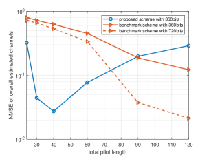
Figure 2: NMSE comparison between quantize-then-estimate and estimate-then-quantize schemes.

Next, we show the gain of our proposed scheme in reducing the pilot transmission overhead and the feedback transmission overhead, respectively. First, Fig. 3 shows the NMSE performance comparison with respect to pilot sequence length when the quantization error and quantization overhead are both ignored under our proposed scheme and the benchmark scheme. It is observed that to achieve the same NMSE performance, our proposed scheme requires a much smaller number of time slots for pilot transmission via utilizing (3) and (4). Second, Fig. 4 shows the NMSE performance comparison with respect to the number of quantization bits, when the noise for receiving the pilot signals at the user side is ignored. Because fewer symbols are quantized under our proposed scheme thanks to the utilization of (3) and (4), our scheme requires a much smaller number of quantization bits to achieve the same NMSE.

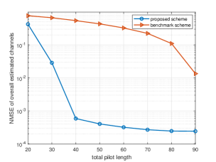
Figure 3: NMSE of performance over pilot sequence length with no quantization noise.

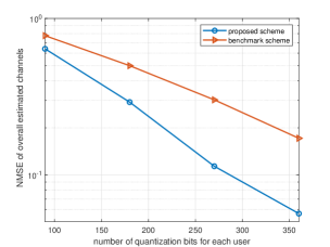
Figure 4: NMSE of performance over number of quantization bits.

VI Conclusions

In this paper, we proposed a novel “quantize-then-estimate” protocol for CSI acquisition in FDD IRS-aided communication. Specifically, all the users feed back the quantized pilot signals to the BS, which can thus leverage the correlation embedded in users’ cascaded channels for channel estimation. We show both analytically and numerically that the overhead for pilot transmission and feedback transmission under our strategy is significantly reduced. Our results open up a new solution for low-overhead communication in IRS-aided systems.

References

- [1] Z. Wang, L. Liu, and S. Cui, “Channel estimation for intelligent reflecting surface assisted multiuser communications: Framework, algorithms, and analysis,” IEEE Trans. Wireless Commun., vol. 19, no. 10, pp. 6607–6620, Oct. 2020.
- [2] Z. Xiong, A. D. Liveris, and S. Cheng, “Distributed Source Coding for Sensor Networks,” IEEE Sig. Process. Mag., vol. 21, no. 5, pp. 80–94, Sep. 2004.
- [3] D. Shen and L. Dai, “Dimension reduced channel feedback for reconfigurable intelligent surface aided wireless communications,” IEEE Trans. Commun., vol. 69, no. 11, pp. 7748–7760, Nov. 2021.
- [4] W. Chen, C.-K. Wen, X. Li, and S. Jin, “Adaptive bit partitioning for reconfigurable intelligent surface assisted FDD systems with limited feedback,” IEEE Trans. Wireless Commun., vol. 21, no. 4, pp. 2488–2505, Apr. 2021.
- [5] N. Jindal, “MIMO broadcast channels with finite-rate feedback,” IEEE Trans. Inf. Theory., vol. 52, no. 11, pp. 5045–5060, Nov. 2006.
- [6] X. Rao and V. K. Lau, “Distributed compressive CSIT estimation and feedback for FDD multi-user massive MIMO systems,” IEEE Trans. Signal Process., vol. 62, no. 12, pp. 3261–3271, Jun. 2014.
- [7] D. J. Love, R. W. Heath, V. K. Lau, D. Gesbert, B. D. Rao, and M. Andrews, “An overview of limited feedback in wireless communication systems,” IEEE J. Sel. Areas Commun., vol. 26, no. 8, pp. 1341–1365, Oct. 2008.
- [8] Y. Yang, B. Zheng, S. Zhang, and R. Zhang, “Intelligent reflecting surface meets OFDM: Protocol design and rate maximization,” IEEE Trans. Commun., vol. 68, no. 7, pp. 4522–4535, Jul. 2020.
- [9] B. Zheng, C. You, and R. Zhang, “Intelligent reflecting surface assisted multi-user OFDMA: Channel estimation and training design,” IEEE Trans. Wireless Commun., vol. 19, no. 12, pp. 8315–8329, Dec. 2020.
- [10] D. Mishra and H. Johansson, “Channel estimation and low-complexity beamforming design for passive intelligent surface assisted MISO wireless energy transfer,” in Proc. IEEE Int. Conf. Acoust. Speech Signal Process. (ICASSP), May 2019.
- [11] H. Alwazani, A. Kammoun, A. Chaaban, M. Debbah, M.-S. Alouini et al., “Intelligent reflecting surface-assisted multi-user MISO communication: Channel estimation and beamforming design,” IEEE Open J. Commun. Soc., vol. 1, pp. 661–680, Jun. 2020.
- [12] A. Gersho and R. M. Gray, Vector quantization and signal compression. Springer Science & Business Media, 1992.
- [13] R. Wang, L. Liu, S. Zhang, and C. Yu, “A new channel estimation strategy in intelligent reflecting surface assisted networks,” in Proc. IEEE Global Commun. Conf. (Globecom), Dec. 2021.