The equation of state of partially ionized hydrogen and deuterium plasma revisited

Abstract

We present novel first-principle fermionic path integral Monte Carlo (PIMC) simulation results for a dense partially ionized hydrogen (deuterium) plasma, for temperatures in the range $15,000$K $\leq T\leq 400,000$K and densities $7\cdot 10^{-7}$g/cm${}^{3}\leq\rho_{H}\leq 0.085$ g/cm³ ($1.4\cdot 10^{-6}$g/cm${}^{3}\leq\rho_{D}\leq 0.17$ g/cm³), corresponding to $100\geq r_{s}\geq 2$, where $r_{s}=\bar{r}/a_{B}$ is the ratio of the mean interparticle distance to the Bohr radius. These simulations are based on the fermionic propagator PIMC (FP-PIMC) approach in the grand canonical ensemble [A. Filinov et al., Contrib. Plasma Phys. 61, e202100112 (2021)] and fully account for correlation and quantum degeneracy and spin effects. For the application to hydrogen and deuterium, we develop a combination of the fourth-order factorization and the pair product ansatz for the density matrix. Moreover, we avoid the fixed node approximation that may lead to uncontrolled errors in restricted PIMC (RPIMC). Our results allow us to critically re-evaluate the accuracy of the RPIMC simulations for hydrogen by Hu et al. [Phys. Rev. B 84, 224109 (2011)] and of various chemical models. The deviations are generally found to be small, but for the lowest temperature, $T=15,640$ K they reach several percent. We present detailed tables with our first principles results for the pressure and energy isotherms.

I Introduction

Warm dense matter (WDM) is a rapidly growing research field on the boarder of plasma physics and condensed matter physics, e.g. Graziani et al. (2014); Fortov (2016); Moldabekov et al. (2018); Dornheim et al. (2018a). Examples include astrophysical objects such as the plasma-like matter in brown and white dwarf stars Saumon et al. (1992); Chabrier (1993); Chabrier et al. (2000), giant planets, e.g. Schlanges et al. (1995); Bezkrovniy et al. (2004); Vorberger et al. (2007); Militzer et al. (2008); Redmer et al. (2011); Nettelmann et al. (2013) and the outer crust of neutron stars Haensel et al. (2006); Daligault and Gupta (2009). In the laboratory, WDM is being routinely produced via laser compression Nora et al. (2015) or with Z-pinches Matzen et al. (2005); Knudson et al. (2015) and, in the near future, also via ion beam compression Ren et al. (2018); Tahir et al. (2019). A particularly exciting application is inertial confinement fusion (ICF) Moses et al. (2009); Hurricane et al. (2016) where recently important breakthroughs have been achieved Abu-Shawareb (2022); Zylstra (2022); Igumenshchev et al. (2023).

In warm dense matter research and ICF, in particular, an accurate description of hydrogen (and deuterium) plays a central role. Hydrogen – the most abundant and, at the same time, the simplest element in the universe – has been in the focus of research for many decades. Its properties have been investigated, among others, in many compression experiments with high intensity lasers, at x-ray free electron laser facilities and at the National Ignition Facility (NIF) at Livermore National Laboratory. Among questions of particular interest are the predicted metal–insulator transition, the hypothetical plasma phase transition and the recently predicted roton feature Dornheim et al. (2018b, 2022); Hamann et al. (2023). Aside from these questions, also basic properties such as the equation of state (EOS), compressibility, optical properties and conductivity are of prime importance for experiments involving hydrogen. However, the accuracy of existing experimental data is still not fully known. The situation is expected to change with upcoming high accuracy experiments including the colliding planar shocks platform at the NIF MacDonald et al. (2023) and the FAIR facility at GSI Darmstadt Tahir et al. (2019).

All this poses particular challenges to theory which comprises a broad arsenal of models and simulation approaches. Even after four decades of research there persist significant deviations among the results of different models, and there remains a surprisingly large scatter of data, even for relatively simple quantities, such as the equation of state. The reason is that the relevant thermodynamic and transport properties of warm dense hydrogen are influenced, among others, by electronic quantum effects, moderate to strong Coulomb correlations, the formation of atoms and molecules, lowering of the ionization and dissociation potentials, and the interaction between charged and neutral species. Available data include (semi-)analytical results within the chemical picture, such as the Pade formulas of Ebeling et al. Ebeling and Richert (1985); Trigger et al. (2003), the Saumon, Chabrier van Horn model Chabrier (1993), the model of Schlanges et al. Schlanges et al. (1995), and the fluid-variational theory of Redmer et al. Juranek et al. (2002), semi-classical molecular dynamics with quantum potentials (SC-MD), e.g. Filinov et al. (2004), electronic force fields Su and Goddard (2007); Ma et al. (2019) and various variants of quantum MD, e.g. Filinov et al. (2002); Knaup et al. (2002); Sjostrom and Daligault (2014); Dai et al. (2010); Kang and Dai (2018). A recent breakthrough occurred with the application of Kohn-Sham density functional theory (DFT) and Born-Oppenheimer MD simulations because they, for the first time, enabled the selfconsistent simulation of realistic warm dense matter, that includes both, plasma and condensed matter phases, e.g. Collins et al. (1995); Plagemann et al. (2012); Witte et al. (2017). Further developments include orbital-free DFT methods (OF-DFT), e.g. Karasiev et al. (2014); Sun et al. (2017) and time-dependent DFT (TD-DFT), e.g. Baczewski et al. (2016).

However, all these methods involve severe approximations – that are related e.g. to the concept of the chemical picture, the semi-classical approximation in MD or the choice of the exchange-correlation functional in DFT – that give rise to systematic errors that are difficult to quantify and that strongly limit the predictive power of the methods. Therefore, a special role is played by first principle computer simulations that – at least in principle – are free of systematic errors and, therefore, may serve as benchmarks and reference for other models. For the thermodynamic quantities of warm dense hydrogen such a role is being played by path integral Monte Carlo (PIMC) simulations, pioneered by D.M. Ceperley and B. Militzer Militzer and Ceperley (2000, 2001a), as well as V.S. Filinov and co-workers, e.g. V.S. Filinov (2000); Filinov et al. (2000, 2001a, 2001b). However, PIMC simulations for warm dense hydrogen are severely hampered by the necessity to accurately treat the Fermi statistics of the electrons. This is known as the fermion sign problem (FSP) that was shown to be N-P hard Troyer and Wiese (2005); Dornheim (2021), i.e. simulations suffer an exponential loss of accuracy with increasing quantum degeneracy of the electrons. For this reason, the computationally expensive direct fermionic PIMC simulations of V.S. Filinov et al., that could use only a limited number of high-temperature factors on the order of $20\dots 50$, became increasingly inaccurate for values of the electron degeneracy parameter $\chi\gtrsim 1$, cf. Eq. (1). An alternative strategy was developed by Ceperley: eliminate the FSP via the fixed node approximation Ceperley (1991, 1996a). This leads to the restricted PIMC (RPIMC) method, and the RPIMC results for hydrogen, including new data Hu et al. (2010, 2011a), still today remain the most reliable reference. The importance of the RPIMC data has grown even more because they have been used by Militzer and co-workers as primary input (in combination with DFT) for extended thermodynamic data tables for hydrogen and a broad set of more complex materials Militzer and Driver (2015).

The magnitude of the systematic error in RPIMC that is introduced by the fixed node approximation is commonly believed to be small. This is, in part, based on the good accuracy of the associated zero-temperature approach (diffusion Monte Carlo), as confirmed by available full CI ground state data. However, the situation is different at finite temperature. While the fixed node approximation in RPIMC has been criticized Filinov (2001, 2014), and occasionally improvements beyond free-particle nodes have been tested Militzer and Pollock (2000); Militzer et al. (2021), so far, no alternative first-principle results have been available that allow one to assess the accuracy and applicability range of the method at finite temperatures. This has changed only recently, when configuration PIMC (CPIMC) simulations have been introduced by Bonitz and co-workers Schoof et al. (2011, 2015a). These are first principle finite temperature PIMC simulations in Fock space that have no sign problem at strong degeneracy and are thus complementary to standard coordinate space PIMC. When applied to the model system of the warm dense uniform electron gas (UEG), the combination of CPIMC with permutation blocking PIMC – coordinate space PIMC that uses fourth-order propagators and determinant sampling – and was introduced by Dornheim (PB-PIMC Dornheim et al. (2015)) made it possible to produce benchmark thermodynamic data with a relative error below $1\%$ Dornheim et al. (2016a); Groth et al. (2016a); Dornheim et al. (2018a). These results were used, among others, to develop finite temperature exchange-correlation functionals for DFT, such as the finite-temperature LDA functional GDSMB Groth et al. (2017). Moreover, these UEG results provided, for the first time, the opportunity to analyze the accuracy of RPIMC simulations in the WDM range. In fact comparison to RPIMC simulations for the UEG of Brown et al. Brown et al. (2013) revealed unexpectedly large errors of the latter exceeding $10\%$ around $r_{s}=1$ Schoof et al. (2015b), for more details, see Refs. Dornheim et al. (2017, 2018a); Filinov et al. (2021).

It is, therefore, of high interest to extend the first-principle direct PIMC simulations to warm dense hydrogen, applying the novel advanced methods that were successfully applied to the UEG before. This will also allow one to benchmark the aforementioned earlier hydrogen simulations and RPIMC, in particular. This is the goal of the present paper. To this end we apply the fermionic propagator PIMC (FP-PIMC) approach – a grand canonical extension of the PB-PIMC method that was recently successfully applied to the thermodynamic properties of the UEG in Ref. Filinov et al. (2021) and to the static density response function and the dynamic structure factor of the UEG Filinov et al. (2023a) and helium 3 Filinov et al. (2023b).

Here we extend the FP-PIMC method to a two-component electron-proton plasma. The approach is formulated in coordinate space and, therefore, the fermion sign problem restricts our simulations to moderate densities, $r_{s}\gtrsim 2$. We present extensive new data for a broad density and temperature range, $r_{s}\in[2;100]$ and $T\in[15,000;400,000]$. Our results include the equation of state, various energy contributions, and pair distributions. Further, we extract approximate data for the degree of ionization and the fraction of molecules. The comparison with earlier results reveals significant inaccuracies of the latter, in particular for low temperatures and/or low densities.

This paper is organized as follows: in Sec. II we recall the main parameters and give a brief overview on selected theoretical data for warm dense hydrogen which will be used for comparison to our results. In Sec. III our FP-PIMC approach is presented and its extension to hydrogen is explained. Section IV presents our numerical results. Detailed data tables for the equation of state and total energy are presented in the appendix.

II Warm dense hydrogen and deuterium

II.1 Relevant parameters

Let us recall the basic parameters of warm dense hydrogen Bonitz (2016); Bonitz et al. (2019):

• The first are the quantum degeneracy parameters, $\theta$ and $\chi$, which involve the Fermi energy $E_{F}$ and the thermal DeBroglie wave length $\lambda$, respectively:

  $$\theta =\frac{k_{B}T}{E_{F}}\,,\quad\chi=n\lambda^{3}\,,$$ (1)

  $$\lambda =\frac{h}{\sqrt{2\pi mk_{B}T}}\,,$$ (2)

  $$E_{F} =\frac{\hbar^{2}}{2m}(3\pi^{2}n)^{2/3}\,,$$ (3)

  where $n$ is the density, $T$ the temperature, and $m$ the particle mass. The proton degeneracy parameter $\chi_{p}$ is a factor $(m_{e}/m_{p})^{3/2}$ smaller than the one of the electrons and is negligible in the parameter range studied in this paper.

• The second parameter is the classical coupling parameter of protons,

  $$\Gamma_{p}=\frac{e^{2}}{ak_{B}T}\,,\quad a^{3}=\frac{4}{3\pi n}\,,$$ (4)

  where $a$ is the mean inter-particle distance.

• Finally, the quantum coupling parameter (Brueckner parameter) of electrons in the low-temperature limit is,

  $$r_{s}=\frac{a}{a_{B}},\quad a_{B}=\frac{\hbar^{2}}{m_{r}e^{2}},\quad m_{r}=\frac{m_{e}m_{p}}{m_{e}+m_{p}},$$ (5)

  where $a_{B}\approx 0.529\AA$ is the Bohr radius, and $m_{r}$ is the reduced mass which, for hydrogen and deuterium, is $m_{r}\approx m_{e}$.

Note that the degeneracy parameters refer to an ideal plasma and give only a rough picture of the physical situation in WDM. At moderate to strong coupling, the spatial extension of electrons may be strongly modified and the physical degeneracy parameter may differ substantially from $\theta$ and $\chi$. Similarly, the presence of bound states significantly alters the physical degeneracy parameters. For a discussion of this effect, see Ref. Filinov et al. (2003a). On the other hand, bound states also significantly affect the coupling strength in the plasma because they lead to a reduction of the number of free particles that interact via the long range Coulomb potential.

II.2 Selected theoretical reference results for warm dense hydrogen

Here we give a brief overview on existing theoretical and simulation results for dense hydrogen and deuterium, see also the discussion in Sec. I. Here we concentrate on those that will be considered for comparison with our simulation results in Sec. IV. For further details on the different methods, the reader is referred to various text books, e.g. Filinov and Bonitz (2006); Fortov (2016); Graziani et al. (2014).

1. by CP2019 we denote the hydrogen EOS by Chabrier et al. Chabrier et al. (2019) that combines simulations from three relevant physical domains, for temperatures below $T\leq 100,000$K:

   i.

   $\rho\leq 0.05$ g/cm³ ($r_{s}\geq 3.8$): the theory of Saumon, Chabrier and van Horn Saumon et al. (1995) in the low-density, low-temperature molecular/atomic phase,

   ii.

   $\rho>10$ g/cm³ ($r_{s}<0.65$): the EOS of Chabrier and Potekhin Chabrier and Potekhin (1998) in the fully ionized plasma (the high-density and high-temperature phase),

   iii.

   $0.3\leq\rho\leq 5$ g/cm³ ($0.8\leq r_{s}\leq 2$) ab initio quantum molecular dynamics calculations Caillabet et al. (2011) at intermediate density and temperature, dominated by pressure dissociation and ionization processes.

   iv.

   For the missing density interval ($2\leq r_{s}\leq 3.8$) spline interpolation of the main thermodynamic quantities is performed that ensures continuity of the quantities and their first two derivatives.

2. by FVT we denote fluid variational theory of Juranek et al. Juranek et al. (2002). There hydrogen is treated as fluid mixture of atoms and molecules, including deviations from linear mixing, and their concentrations are obtained by self-consistent solutions of non-ideal Saha equations. That reference states reasonable accuracy for $\rho\lesssim 0.6$ g cm^-3.

3. by WREOS we denote the wide-range EOS of Wang and Zhang, Ref. Wang and Zhang (2013). They combine ab initio Kohn-Sham DFT-MD, for $\theta<1$ with orbital-free DFT simulations, for $\theta>1$.

4. by HXCF we denote the equation of state table of deuterium of Mihaylov et al., Ref. Mihaylov et al. (2021). It aims at a universal DFT-based treatment for all temperatures and densities including high-order exchange-correlation functionals and also path integral MD (PIMD) data. The data points for $r_{s}=17.53$ (deuterium density $\rho_{D}=0.001$g cm^-3) that are included in the figures below have been obtained by Kohn-Sham MD (based on PIMD).

5. by RPIMC we denote results from restricted (fixed nodes) PIMC simulations and RPIMC-DFT combinations, see also Sec. I, for a discussion. In Ref. Militzer et al. (2021) a first-principles equation of state database was provided which will be used for comparison throughout this work. While these tables are given for many materials and contain combinations of RPIMC data with DFT-LDA simulations, for hydrogen only RPIMC data are involved Militzer et al. (2021).

The above selection of the different hydrogen equations of state is by no means representative. The goal is to compare our new PIMC data with recent results that are frequently used in astrophysics or warm dense matter research and for which reference data for the same temperatures have been published so interpolation can be avoided.

In our opinion, among the data above, the RPIMC-based ones are the most reliable because they do not involve any sources of systematic errors – except for the choice of the nodes in the fixed node approximation. On the other hand, many other equations of state involve RPIMC data, in one way or the other. For these reasons, the comparison with RPIMC is in the focus of the analysis of our new simulation data. Since our FP-PIMC simulations do not involve any approximation, such as fixed nodes, we expect them to be more reliable as RPIMC and, in case of deviations between the two, the origin should be in the nodes of RPIMC. The main source of error in FP-PIMC is of statistical nature, for these reasons we devote special attention to verify convergence of our results.

III Overview on the present direct fermionic PIMC simulations

III.1 Fermionic propagator PIMC (FP-PIMC)

We use Feynman’s path integral picture of quantum mechanics where particles are represented by coordinate space-imaginary time “trajectories”. Fermions with different spin projections are denoted by the coordinate vector $\mathbf{R}^{s}_{p}=(\mathbf{r}^{s}_{1,p},\ldots,\mathbf{r}^{s}_{N^{s},p})$ with $\{s=\uparrow,\downarrow\}$, and the ions by the vector $\mathbf{R}^{I}_{p}$. The ensemble of the particle trajectories in the imaginary time is denoted by the variable $\mathbf{X}^{s(I)}=(\mathbf{R}^{s(I)}_{1},\ldots,\mathbf{R}^{s(I)}_{P})$, where the lower index indicates the imaginary time argument, $\tau_{p}=p\epsilon$ with $\epsilon=\beta/P$ and $0\leq p\leq P$. Here, $P\geq 1$ denotes the number of high-temperature factors (“time slices”) in the path integral formalism, see below.

To evaluate the fermionic partition function, the sum over $N_{s}!$ permutations is performed explicitly, which contains sign-alternating terms, where the sign $\text{Sgn}(\sigma_{s})=\pm 1$ depends on the parity of the permutation in each of the two spin-subspaces:

$$Z_{F}= (N^{\uparrow}!N^{\downarrow}!)^{-1}\sum\limits_{p\in\wp}\int\text{d}\mathbf{X}^{\uparrow}\text{d}\mathbf{X}^{\downarrow}\text{d}\mathbf{X}^{I}\prod\limits_{p=1}^{P}\text{Sgn}(\sigma_{\uparrow})\text{Sgn}(\sigma_{\downarrow})$$

$$\times\lvert\langle\mathbf{R}_{p-1}|e^{-\epsilon\hat{H}}|\hat{\pi}_{\sigma_{\uparrow}}\hat{\pi}_{\sigma_{\downarrow}}\mathbf{R}_{p}\rangle\rvert\,,$$ (6)

where we introduced the notation $\mathbf{R}_{p}=(\mathbf{R}^{\uparrow}_{p},\mathbf{R}^{\downarrow}_{p},\mathbf{R}^{I}_{p})$, and the sum over $p\in\wp$ runs over different permutation classes. In this representation, called the direct path-integral Monte Carlo (DPIMC) method, physical expectation values are evaluated with the statistical error

$$\langle A\rangle=\frac{\left\langle\hat{A}\cdot\prod\limits^{s}\text{Sgn}(\sigma_{s})\right\rangle}{\langle s\rangle}\pm\delta A,\quad\delta A\sim 1/\langle s\rangle\,,$$ (7)

which scales inversely proportional to the average sign

$$\langle s\rangle=\left\langle\prod\limits^{s}\text{Sgn}(\sigma)\right\rangle=\frac{Z_{F}}{Z_{B}}=e^{-\beta N(f^{F}-f^{B})}\,.$$ (8)

The sign decays exponentially with particle number $N$, inverse temperature $\beta$ and the free energy difference of bosons and fermions.

To recover the effect of the exchange-correction hole as observed by the interaction of two spin-like fermions, one important improvement to the DPIMC sampling (6) is necessary. This physical effect can be reproduced in numerical simulations by the use of anti-symmetric propagators (determinants) already on the level of stochastic importance sampling of particle trajectories. This requires to introduce a modified partition function where the summation over different permutation classes is performed analytically in the kinetic energy part of the density matrix (DM), and results in the Slater determinant constructed from the free-particle propagators

$$Z_{F}=\frac{1}{N^{\uparrow}!N^{\downarrow}!}\int\text{d}\mathbf{X}^{\uparrow}\text{d}\mathbf{X}^{\downarrow}\text{d}\mathbf{X}^{I}\prod\limits_{p=1}^{P}\text{Sgn}_{p}\,e^{-S^{A}_{p}}$$ (9)

$$\text{Sgn}_{p}=\text{Sgn}\det\mathbb{M}^{\uparrow}_{p-1,p}\cdot\text{Sgn}\det\mathbb{M}^{\downarrow}_{p-1,p},$$ (10)

$$e^{-S^{A}_{p}}=e^{-\epsilon U(\mathbf{R}_{p-1},\mathbf{R}_{p})}e^{W_{\text{ex}}(\mathbf{R}_{p-1},\mathbf{R}_{p})},$$ (11)

$$W_{\text{ex}}=\ln\lvert\det\mathbb{M}^{\uparrow}_{p-1,p}\rvert+\ln\lvert\det\mathbb{M}^{\downarrow}_{p-1,p}\rvert,$$ (12)

where the off-diagonal “action”, $S^{A}_{p}$, depends on the interaction term $U$ between charged particles on two successive time slices ($p-1,p$), while $W_{\text{ex}}$ accounts for exchange effects due to Fermi statistics via the Slater determinants.

The fermionic (anti-symmetric) free-particle (FFP-) propagator between two adjacent time slices is given by

$$D_{p-1,p}^{s}=\sum\limits_{\sigma_{s}}\left\langle\mathbf{R}^{s}_{p-1}\left|e^{-\epsilon\hat{K}}\right|\hat{\pi}_{\sigma_{s}}\mathbf{R}^{s}_{p}\right\rangle=\frac{\det\mathbb{M}^{s}_{p-1,p}}{\lambda^{DN^{s}}_{\epsilon}},$$ (13)

where the spin components are denoted by $s=\uparrow,\downarrow$, and $\mathbf{M}^{s}$ is the $N^{s}\times N^{s}$ anti-symmetric diffusion matrix

$$\mathbb{M}^{s}=||m_{kl}(p-1,p)||,\quad k,l=1,\ldots N^{s}\,,$$ (14)

$$m_{kl}(p-1,p)=\exp\left(-\frac{\pi}{\lambda^{2}_{\epsilon}}[\mathbf{r}^{s}_{l,p}-\mathbf{r}^{s}_{k,p-1}]^{2}\right)\,.$$ (15)

This representation has several advantages. First, the resulting density matrix is anti-symmetric with respect to any pair exchange of same spin fermions. Second, the probability of micro-states is now proportional to the value of the Slater determinants, and the degeneracy of the latter, at small particle separations, correctly recovers the Pauli-blocking effect. Third, the FFP-propagators partially reduce the fermion sign-problem (FSP).

The change of the sign of the Slater determinants, evaluated along the imaginary time interval, $0\leq\tau_{p}\leq\beta$, is taken into account by the extra factors, $\text{Sgn}_{p}$. Combined together they define the average sign in fermionic PIMC,

$$\langle S\rangle=\left\langle\prod\limits_{p=1}^{P}\text{Sgn}\,\det\mathbb{M}^{\uparrow}_{p-1,p}\cdot\text{Sgn}\det\mathbb{M}^{\downarrow}_{p-1,p}\right\rangle,$$ (16)

and characterize the efficiency of simulations in terms of the statistical error $\delta A$ in Eq. (7). The PIMC simulations become hampered by the FSP Ceperley (1996b); Troyer and Wiese (2005) once the statistical uncertainties are strongly enhanced due to an exponential decay of the average sign $\langle S(N,\beta)\rangle$ with the particle number $N$, the inverse temperature $\beta=1/k_{B}T$ or the degeneracy parameter, $\theta$ (or $\chi$). The usage of the fermionic propagators, Eq. (13), permits to partially overcome the sign problem and make the simulations feasible up to $\chi\lesssim 3$.

The efficiency of the fermionic propagator approach has been demonstrated by several authors, including Takahashi and Imada Takahashi and Imada (1984), V. Filinov and co-workers Filinov et al. (2001a, c); Bonitz et al. (2005) and Lyubartsev Lyubartsev (2005). Chin Chin (2015) used determinant propagators to simulate relatively large ensembles of electrons in 3D quantum dots. The PB-PIMC simulations by Dornheim et al. Dornheim et al. (2015, 2018a) have addressed the thermodynamic proprieties of the UEG from first principles.

III.2 Quantum pair potentials in plasma simulations

Before discussing our plasma simulations, we review the concept of effective quantum potentials that are used to overcome the divergence of the attractive Coulomb potential which leads to divergencies in classical statistical thermodynamics. Taking quantum effects into account gives rise to modified pair potentials which do not exhibit these singularities anymore. Such potentials have been derived by Kelbg Kelbg (1963a, b, 1964), Deutsch Deutsch and Lavaud (1972) and others. They capture the basic quantum diffraction effects and are exact in the weak coupling limit. Furthermore, an improved version of the Kelbg potential (IKP) was derived Filinov et al. (2004, 2003a) that extends the applicatbility range beyond the weak coupling limit, as will be discussed below. In Eq. (17) we reproduce the IKP whereas the original Kelbg potential follows from it by setting the parameter $\gamma_{ij}$ equal to one.

$$U(r,\lambda_{ij})=\frac{Z_{q}}{r}\left[1-e^{-\frac{r^{2}}{\lambda_{ij}^{2}}}+\frac{\sqrt{\pi}r}{\lambda_{ij}\gamma_{ij}}\left(1-\operatorname{erf}\left[\frac{\gamma_{ij}r}{\lambda_{ij}}\right]\right)\right],$$

$$Z_{q}=q_{i}q_{j},\quad\lambda_{ij}^{2}=\frac{\hbar^{2}\beta}{2\mu_{ij}},\quad\frac{1}{\mu_{ij}}=\frac{1}{m_{i}}+\frac{1}{m_{j}}\,,$$ (17)

and was obtained via first-order perturbation theory. Quantum effects related to the finite extension of particles on the length scale of the de-Broglie wavelength, $\lambda_{ij}$, which depends on temperature and the reduced mass, enter explicitly.

This potential has the advantage of preserving the correct first derivative of the the exact binary Slater sum $S_{ij}(r)$ at zero interparticle distance. However, it does not include strong coupling effects, in particular it does not include bound states, which become important at low temperatures. This drawback has been corrected with the introduction of the improved Kelbg potential (IKP) by A. Filinov et al. Filinov et al. (2003b, 2004). The correction parameter $\gamma_{ij}$ in Eq. (17) is directly related to the exact Slater sum at zero distance

$$\gamma_{ij}(\beta,\mu_{ij})=-\frac{\sqrt{\pi}}{\lambda_{ij}}\frac{Z_{q}\beta}{\ln[S_{ij}(r_{ij}=0,\beta)]}\,.$$ (18)

A detailed discussion of the accuracy of the IKP, Eq. (17), for all types of binary Coulomb interactions, and practical applications for a hydrogen plasma in both, PIMC and MD simulations was presented in Ref. Filinov et al. (2004).

In our recent work Bonitz et al. (2023) we performed detailed accuracy and convergence tests, being relevant for the present plasma simulations. First, we performed FP-PIMC simulations with the IKP and compared them to simulations where the exact off-diagonal pair potential (see next Sec. III.3) for the electron-ion interaction Ceperley (1995a) (defined by the exact Slater sum) was employed. In summary, we found that, while the IKP allows to accurately describe the electron-electron (ion-ion) correlation effects, its accuracy given by the diagonal approximation to the off-diagonal pair density matrix

$$\rho(\mathbf{r},\mathbf{r}^{\prime};\tau)\approx\frac{1}{2}\left[\rho(\mathbf{r},\mathbf{r};\tau)+\rho(\mathbf{r}^{\prime},\mathbf{r}^{\prime};\tau)\right]\,,$$ (19)

is not sufficient. The IKP exhibits very slow convergence with respect to the number of high-temperature propagators $P$, as was shown in Ref. Bonitz et al. (2023). Additional extensive tests of the $P$-convergence in the present FP-PIMC simulations, including the dependence on the system size, will be summarized in Sec. IV.1.

III.3 Combination of the fourth-order factorization scheme with the product density matrix ansatz

As shown in the previous discussion, while it is sufficient to use the fitted IKP for the binary interactions $ij=ee,ii$, a more accurate treatment of the attractive electron-ion interaction is required to reduce the number of factors, $P$, to a moderate value. This is crucial because the efficiency of FP-PIMC sensitively depends on the imaginary time step $\epsilon=\beta/P$. A larger time step (smaller $P$-value) in the high-temperature factorization increases the average sign $\langle S\rangle$ in Eq. (16) and extends the applicability range of fermionic simulations to higher degeneracy. To achieve this goal – without loss of accuracy – as was done in the UEG case Filinov et al. (2021); Dornheim et al. (2015), we take advantage of the fourth-order factorization scheme proposed by Chin et al. Chin and Chen (2002) and Sakkos et al. Sakkos et al. (2009):

$$e^{-\beta\hat{H}}=\prod\limits_{p=1}^{P}e^{-\epsilon(\hat{K}+\hat{V})}$$ (20)

$$\approx\prod\limits_{p=1}^{P}e^{-\epsilon\hat{W}_{1}}e^{-t_{1}\epsilon\hat{K}}e^{-\epsilon\hat{W}_{2}}e^{-t_{1}\epsilon\hat{K}}e^{-\epsilon\hat{W}_{1}}e^{-t_{0}\epsilon\hat{K}}+O(\epsilon^{4})\,.$$

The potential and the kinetic energy contributions along the imaginary time step $\epsilon$ are divided into three parts as, $t_{1}\epsilon+t_{1}\epsilon+t_{0}\epsilon=\epsilon$, with $t_{0}$ being a free parameter which influences the $P$-convergence. As a result the higher order commutators between $\hat{K}$ and $\hat{V}$ exactly cancel, up to the order $O(\epsilon^{4})$ Suzuki (1985). Thereby the effective total number of factors in Eq. (9) becomes $3P$, which has to be taken into account in the cited $P$-values in Sec. IV.1.

The new potential energy operators introduced in (20) take the form Chin and Chen (2002)

$$\hat{W}_{1}=v_{1}\hat{V}+u_{0}a_{1}\hat{W}_{Q},$$ (21)

$$\hat{W}_{2}=v_{2}\hat{V}+u_{0}a_{2}\hat{W}_{Q},\quad a_{2}=1-2a_{1}$$ (22)

$$\hat{W}_{Q}=\epsilon^{2}[[\hat{V},\hat{K}],\hat{V}]=\frac{\hbar^{2}}{m}\epsilon^{2}\sum\limits_{i=1}^{N}\lvert\mathbf{F}_{i}^{2}\rvert,$$ (23)

where $\mathbf{F}_{i}$ is the full force acting on a particle “i”. The involved coefficients are defined as

$$v_{1}=\frac{1}{6(1-2t_{0})^{2}},\;v_{2}=1-2v_{1},\;2t_{1}=1-t_{0},$$ (24)

$$u_{0}=\frac{1}{12}\left[1-\frac{1}{1-2t_{0}}+\frac{1}{6(1-2t_{0})^{3}}\right].$$ (25)

The choice $t_{0}=1/6$ (as used here), in particular, corresponds to an equidistant time-step in Eq. (20), and a symmetric action of the diffusion operator $e^{-t_{1}\epsilon\hat{K}}$.

Below we proceed with an explicit derivation of the combination of this scheme with the pair product ansatz (PPA) for the N-particle density matrix introduced by Pollock and Ceperley Ceperley (1995a) which was efficiently employed in the many RPIMC simulations Brown et al. (2013); Militzer and Pollock (2000); Militzer and Ceperley (2001a); Hu et al. (2011b); Militzer et al. (2021).

Let us explicitly write the contribution of binary interactions in the N-body density operator of a two-component system composed of electrons (e) and ions (I)

$$e^{-\epsilon\hat{H}}=e^{-\epsilon(\hat{K}_{e}+\hat{K}_{I}+\hat{V}_{ee}+\hat{V}_{II}+\hat{V}_{eI})},$$ (26)

where each operator is the sum of one-particle or two-particle operators. Later we will explicitly use the large mass asymmetry of the species, $m_{I}/m_{e}\gg 1$. Now we apply the fourth-order factorization result (20) with redefined (non-commuting) operators

$$\hat{\bar{K}}=\hat{K}_{e}+\hat{K}_{I}+\hat{V}_{eI},$$ (27)

$$\hat{\bar{V}}=\hat{V}_{ee}+\hat{V}_{\text{II}}\,,$$ (28)

and evaluate the additional quantum corrections, $\hat{W}_{Q}$, to the bare operator $\hat{\bar{V}}$ by Eq. (21)–(23). After omitting all mutually commuting operators we are left with the final result

$$\hat{\bar{W}}_{Q}=\hat{W}_{ee,Q}+\hat{W}_{II,Q},$$ (29)

$$\hat{W}_{ee,Q}=\frac{\hbar^{2}}{m_{e}}\epsilon^{2}\sum\limits_{i=1}^{N_{e}}\lvert\mathbf{F}_{e,i}^{2}\rvert,$$ (30)

$$\hat{W}_{II,Q}=\frac{\hbar^{2}}{m_{I}}\epsilon^{2}\sum\limits_{j=1}^{N_{I}}\lvert\mathbf{F}_{I,j}^{2}\rvert,$$ (31)

where $\mathbf{F}_{e(I),i}$ is the full force acting on particle “i” only from the same particle species [i.e. with the exclusion of the e-i interaction]. The corresponding matrix elements are diagonal in the coordinate representation

$$\langle\mathbf{R}_{p-1}|e^{-\epsilon\hat{\bar{W}}_{n}}|\mathbf{R}_{p}\rangle=e^{-\epsilon W(\mathbf{R}_{p})}\,\delta(\mathbf{R}_{p}-\mathbf{R}_{p-1})\,,$$ (32)

$$W=-\frac{1}{2}\epsilon\,\left[\bar{W}_{n}(\mathbf{R}_{p-1};\tau_{p-1})+\bar{W}_{n}(\mathbf{R}_{p};\tau_{p})\right],$$ (33)

$$\bar{W}_{n}=v_{n}(V_{ee}+V_{II})+u_{0}a_{n}(W_{ee,Q}+W_{II,Q}).$$ (34)

In particular, the $ee$-correlations are treated in the fourth-order factorization scheme the same as in the UEG case Dornheim et al. (2015); Filinov et al. (2021). As an alternative approach to Chin’s result, Eqs. (21)–(23), we can include first quantum corrections via the effective quantum potentials, e.g. the IKP (see Sec III.2). Note that a direct use of the IKP in Eqs. (21)–(23) is not justified as this would lead to double counting of quantum diffraction effects.

Hence, for particles with the same charge and mass we benefit from the fast $P$-convergence of Chin’s scheme in a one-component system Sakkos et al. (2009); Dornheim et al. (2015); Filinov et al. (2021). However, this scheme will fail for two electrons with different spins, once, at low temperature/high density, they closely approach each other, e.g. within a molecule or by scattering of two neutrals, cf. Fig. 1c. This behavior will be prohibited by a divergent Coulomb force in Eq. (23), unless a tiny time-argument $\epsilon$ is employed. Therefore, for plasma simulations we use a hybrid scheme: $V_{ee}^{\uparrow\uparrow},V_{ee}^{\downarrow\downarrow}$ and $V_{II}$ are treated via Eqs. (21)–(23), whereas $V_{ee}^{\uparrow\downarrow}$ is treated via the IKP (17) with the fit parameter $\gamma_{ee}(\epsilon,\mu_{ee})$ Filinov et al. (2003a).

To complete our result, we proceed with the evaluation of the second operator (diffusion operators plus the electron-ion contribution). To shorten the notations we use $\epsilon\equiv t_{n}\epsilon\;(n=0,1)$:

$$\rho(\mathbf{R}_{p-1},\mathbf{R}_{p},\epsilon)=\langle\mathbf{R}_{p-1}|e^{-\epsilon\hat{\bar{K}}}|\mathbf{R}_{p}\rangle\approx$$

$$\int\text{d}\mathbf{R}_{p}^{\prime}\,\langle\mathbf{R}_{p-1}|e^{-\epsilon(\hat{K}_{e}+\hat{V}_{eI}})|\mathbf{R}_{p}^{\prime}\rangle\langle\mathbf{R}_{p}^{\prime}|e^{-\epsilon\hat{K}_{I}}|\mathbf{R}_{p}\rangle.$$ (35)

In the second line we employed a first approximation, and neglected the commutator term, $\epsilon^{2}[\hat{V}_{eI},\hat{K}_{I}]$, which is justified by the nearly classical behavior of ions.

In the second step, we use the PPA, with the explicit result, $|\mathbf{R}^{\prime\,e}_{p}\rangle=|\mathbf{R}_{p}^{e}\rangle$, which follows from the fact that the diffusion operator (in the second term) acts only on the ion variables. This allows us to simply the first term to

$$\langle\mathbf{R}_{p-1}|e^{-\epsilon(\hat{K}_{e}+\hat{V}_{eI})}|\mathbf{R}_{p}^{\prime}\rangle=$$

$$\langle\mathbf{R}_{p-1}^{I}|\mathbf{R}_{p}^{\prime\,I}\rangle\times\rho^{e}_{0}(\mathbf{R}_{p-1}^{e},\mathbf{R}^{e}_{p},\epsilon)\,\times$$

$$\prod\limits_{i=1}^{N_{e}}\prod\limits_{j=1}^{N_{I}}\exp{\left[-\epsilon\,U_{eI}(\mathbf{r}^{ij}_{p-1},\mathbf{r}^{ij}_{p})\right]},$$ (36)

$$\mathbf{r}^{ij}_{p-1}=\lvert\mathbf{r}^{i,e}_{p-1}-\mathbf{r}^{j,I}_{p-1}\rvert,\quad\mathbf{r}^{ij}_{p}=\lvert\mathbf{r}^{i,e}_{p}-\mathbf{r}^{j,I}_{p-1}\rvert\,,$$ (37)

After performing the integral over $\mathbf{R}_{p}^{\prime}$, we get our final result for the DM in Eq. (35)

$$\rho(\mathbf{R}_{p-1},\mathbf{R}_{p},\epsilon)=$$

$$\rho^{e}_{0}(\mathbf{R}_{p-1}^{e},\mathbf{R}^{e}_{p},\epsilon)\times\rho^{I}_{0}(\mathbf{R}_{p-1}^{I},\mathbf{R}^{I}_{p},\epsilon)$$

$$\times\prod\limits_{i=1}^{N_{e}}\prod\limits_{j=1}^{N_{I}}\exp{\left[-\epsilon\,U_{eI}(\mathbf{r}^{ij}_{p-1},\mathbf{r}^{ij}_{p})\right]}\,,$$ (38)

where $\rho_{0}^{e}$ and $\rho_{0}^{I}$ are the $N$-body free-particle DM for electrons and ions, and $U_{eI}$ is the exact pair potential for the electron-ion problem. An explicit numerical scheme to evaluate $U_{eI}$ was proposed by Storer and Klemm Storer (1968); Klemm and Storer (1973), and a parametrization was introduced by Pollock Pollock (1988) and Ceperley Ceperley (1995a). Its diagonal approximation via (19), at high temperatures, converges to the IKP Filinov et al. (2004), but is more accurate for $T\lesssim 1Ry$.

The above derivation by its physical assumptions resembles the adiabatic approximation but applied at the “elevated” (via the factorization) higher temperature $T\sim\epsilon^{-1}$. The thermal fluctuations in the ion trajectory propagating from $|\mathbf{R}_{p}^{I}\rangle$ to $|\mathbf{R}_{p}^{\prime\,I}\rangle$ are induced by the diffusion operator $e^{-\epsilon\hat{K}_{I}}$, and are of the order of the ion DeBroglie wavelength $\lambda_{I}(\epsilon)$, Eq. (2). This length scale should be much smaller than the Bohr radius – the characteristic spatial range of the e-i interaction. In this case the interaction energy in the DM can be approximated in different ways, cf. $V_{eI}(\lvert\mathbf{r}^{e}_{p}-\mathbf{r}^{\prime\,I}_{p}\rvert)\approx V_{eI}(\lvert\mathbf{r}^{e}_{p}-\mathbf{r}^{I}_{p}\rvert)\approx V_{eI}(\lvert\mathbf{r}^{e}_{p}-\mathbf{r}^{I}_{p-1}\rvert)$.

In the final step, the free-particle electron DM should be antisymmetrized as in Eq. (9). This can be done by splitting the e-i pair potential into a diagonal (D) and an off-diagonal (OD) contribution

$$U_{eI}(\mathbf{r}_{p-1},\mathbf{r}_{p};\epsilon)=$$

$$\frac{1}{2}\left[u^{D}_{\epsilon}(\mathbf{r}_{p-1})+u^{D}_{\epsilon}(\mathbf{r}_{p})\right]+u^{\text{OD}}_{\epsilon}(\mathbf{r}_{p-1},\mathbf{r}_{p}).$$ (39)

By performing, as before, the summation over permutations in Eq. (6), we obtain the same representation for the partition function as in (9) with the following modifications:

First, the number of imaginary time slices in the particle trajectories is changed $P\rightarrow 3P$, due to the 4th-order representation (20) [we perform two additional diffusion steps weighted by the interactions $\hat{W}_{1(2)}$];

Second, the anti-symmetric diffusion matrix now includes the off-diagonal part of the e-i pair potential directly in the matrix elements

$$\mathbb{M}^{s,\text{int}}=||m_{kl}^{\text{int}}(p-1,p)||,\quad k,l=1,\ldots N^{s}\,,$$ (40)

$$m_{kl}^{\text{int}}(p-1,p)=$$

$$\exp\left(-\frac{\pi}{\lambda^{2}_{\epsilon}}[\mathbf{r}^{s}_{l,p}-\mathbf{r}^{s}_{k,p-1}]^{2}-\epsilon\sum\limits_{j=1}^{N_{I}}u^{\text{OD}}_{\epsilon}(\mathbf{r}_{p-1}^{kj},\mathbf{r}_{p}^{lj})\right)\,,$$

where the sum runs over all ions, and the vectors $\{\mathbf{r}_{p-1}^{kj}$,$\mathbf{r}_{p}^{lj}\}$ specify the e-i distances on two successive time slices. Note, that in the Slater determinant all electron coordinates are permuted, and each electron does not need to be specified by a distinguished trajectory, as in PIMC for Bose systems Ceperley (1995a) or in RPIMC Ceperley (1991);

Third, the potential energy part is now diagonal and includes several contributions [the arguments are defined as $x=(\mathbf{R}_{p-1},\mathbf{R}_{p-1};t_{n}\epsilon)$ and $x^{\prime}=(\mathbf{R}_{p},\mathbf{R}_{p};t_{n}\epsilon)$]:

1. Due to 4th-order factorization,

   $$U^{\text{4th}}(x,x^{\prime})=\frac{1}{2}\left[W(x)+W(x^{\prime})\right],$$ (41)

   $$W(x)=W_{ee}^{\uparrow\uparrow}(x)+W_{ee}^{\downarrow\downarrow}(x)+W_{\text{II}}(x),$$ (42)

2. The IKP potential for the opposite spin electrons

   $$U_{ee}^{\uparrow\downarrow}(x,x^{\prime})=\frac{1}{2}\left[U_{ee}^{IKP}(x)+U_{ee}^{IKP}(x^{\prime})\right],$$ (43)

   or, alternatively, we use the diagonal part $u_{\epsilon}^{D}$ of the exact pair potential for two electrons, similar to Eq. (39).

3. The e-i interaction is included via the diagonal part of the e-i pair potential

   $$U^{\text{D}}_{eI}(x,x^{\prime})=\frac{1}{2}\left[u^{D}(x)+u^{D}(x^{\prime})\right].$$ (44)

4. The off-diagonal contributions to the ei-interaction are explicitly included in the Slater determinants, and account for the indistinguishable nature of the same spin electrons.

Note, that only the 4th-order factorization includes the bare Coulomb potential, whereas the other effective potentials, $U^{\uparrow\downarrow}$ and $U_{eI}$, are soft and permit formation of bound states even with only a few high-temperature factors involved, e.g. $P\sim 3$.

With the above derivation, we have achieved our main goal: exchange effects related to the electron spin are taken into account via the anti-symmetric short-time propagators (40) in the form of Slater determinants modified by e-i correlations.

III.4 Thermodynamic functions

In this section we present the estimators for the main thermodynamic functions of interest used in our FP-PIMC approach. We start from the definition of the partition function,

$$Z=\int\text{d}\mathbf{X}\int\prod\limits_{p=1}^{P}e^{-\epsilon_{p}U(\mathbf{R}_{p})}\det\mathbb{M}[\rho_{0}(\mathbf{R}_{p-1},\mathbf{R}_{p};\tau)]\,,$$

where, $\mathbf{R}_{p}=(\mathbf{r}_{1,p},\mathbf{r}_{2,p},\ldots,\mathbf{r}_{N,p})$, contains the coordinates of all particles. Compared to the exact representation, cf. Eqs. (9), (34)–(40), and (21)–(23) we have simplified the notations to highlight the general structure of the related thermodynamic estimators. For example, the single determinant represents the contributions of two Slater determinants (for the spin up/down electrons). The explicit expressions of the total, kinetic and potential energy for the 4th-order factorization is re-derived with additional contributions from the quantum correction, $\hat{W}_{Q}$ (23), for details see Sakkos et al. Sakkos et al. (2009). Also the summation over $P$ should be extended to $3P$ due to additional factorization factors in (20).

The total interaction energy $U$ is the sum of the pair potentials of particles of the same kind and between different species,

$$U(\mathbf{R}_{p})=\sum_{\alpha}\sum_{i<j}^{N_{\alpha}}u_{\alpha\alpha}(\mathbf{r}^{ij}_{p})+\sum_{\alpha}\sum_{\beta}\sum\limits_{i=1}^{N_{\alpha}}\sum\limits_{j=1}^{N_{\beta}}u_{\alpha\beta}(\mathbf{r}^{ij}_{p})\,.$$ (45)

III.4.1 Pressure

The pressure is related to the partition function via

$$\beta p=\frac{\partial\ln Z}{\partial V}\,,$$ (46)

where the derivative is performed by introducing a scaling factor, $\alpha=L/L_{0}=(V/V_{0})^{1/3}$, and by re-scaling all particle coordinates, $\mathbf{r}\rightarrow\alpha\mathbf{r}$,

$$\frac{\partial\ln Z}{\partial V}=\left[\frac{\partial\ln Z(\alpha\mathbf{X})}{\partial\alpha}\frac{\alpha}{3V}\right]_{\alpha=1}.$$ (47)

This standard procedure, applied within the FP-PIMC representation of the $N$-body DM, leads to several contributions which originate from its kinetic and potential parts, as well as additional terms, in the case of quantum potentials, such as the (improved) Kelbg potential, Eq. (17).

The interaction-induced contribution to the pressure is obtained as the $\alpha$-derivative of the potential energy term with the substitution $\{\mathbf{x}_{i}=\alpha\mathbf{r}_{i},\;\;i=1,\dots N\}$

$$\frac{\partial U(\mathbf{X}_{p})}{\partial\alpha}=\sum\limits_{i<j}\sum\limits_{d=1}^{3}\left[\frac{u(\mathbf{x}_{p}^{ij})}{\partial x_{p}^{ij,d}}\frac{\partial x_{p}^{ij,d}}{\partial\alpha}\right]_{\alpha=1}=\sum\limits_{i<j}^{N}\nabla u(\mathbf{r}_{p}^{ij})\cdot\mathbf{r}_{p}^{ij}$$

and leads to an analogous result as in classical Statistical Physics, with an additional averaging along the particle trajectories

$$p^{V}=-\frac{1}{3V}\left\langle\frac{1}{P}\sum\limits_{p=1}^{P}\sum\limits_{i<j}^{N}\nabla u(\mathbf{r}_{p}^{ij})\cdot\mathbf{r}_{p}^{ij}\right\rangle\,,$$ (48)

with $\mathbf{r}^{ij}_{p}=\mathbf{r}_{i,p}-\mathbf{r}_{j,p}$, where the coordinate vectors $\mathbf{r}_{i,p}=\mathbf{r}_{i}(\tau_{p})$ depend on the imaginary time argument, $0\leq\tau_{p}\leq\beta$, with $1\leq p\leq P$.

The long-range interactions with the periodically repeated main simulation cell are evaluated either via the Ewald summation or the angle-averaged Yakub potential (“Y”) Yakub and Ronchi (2005) which gives rise to additional contributions. We have tested both potentials and found that, for the simulation parameters used in this paper, the results for both are practically indistinguishable. For the case of the Yakub potential the long-range interaction term

$$u_{t}^{Y}(\mathbf{r}^{ij}_{p})=\frac{2\pi}{3V}r_{p}^{2},$$ (49)

gives rise to the tail correction to the pressure

$$p_{1}^{Y}=\left\langle\frac{1}{P}\sum\limits_{p=1}^{P}\sum\limits_{i<j}^{N}\frac{\partial u^{Y}_{t}(x^{ij}_{p})}{\partial\alpha}|_{\alpha=1}\right\rangle=\left\langle-\left[\frac{3}{\alpha}u^{Y}_{t}(r^{ij}_{p})\right]_{\alpha=1}\right\rangle$$

and an additional contribution to the virial part

$$p_{2}^{Y}=\frac{1}{V}\left\langle\frac{1}{P}\sum\limits_{p=1}^{P}\sum\limits_{i<j}^{N}\nabla u^{Y}_{t}(\mathbf{r}^{ij}_{p})\cdot\mathbf{r}^{ij}_{p})\right\rangle\,.$$ (50)

Next, we take into account the contribution of the kinetic energy part (constructed with the Slater determinants between adjacent time slices $\{\tau_{p-1},\tau_{p}\}$)

$$p^{T}=\frac{1}{3V}3Nk_{B}T\cdot P+$$ (51)

$$\left\langle\frac{1}{3VP}\sum\limits_{p=1}^{P}\frac{\partial\det\mathbb{M}[\rho(\alpha\mathbf{R}_{p-1},\alpha\mathbf{R}_{p}]/\partial\alpha}{\det\mathbb{M}[\rho(\mathbf{R}_{p-1},\mathbf{R}_{p}]}\right\rangle\,.$$

Alternatively, using the result for the $\alpha$-derivative of the matrix elements in $\mathbb{M}[m_{kl}]$

$$\left[\frac{\partial m_{kl}(\alpha\mathbf{r}_{k,p-1},\alpha\mathbf{r}_{l,p})}{\partial\alpha}\right]_{\alpha=1}=m_{kl,p}^{0,\alpha},$$ (52)

$$m_{kl,p}^{0,\alpha}=-\frac{2}{\lambda^{2}_{\tau_{p}}}\left(\mathbf{r}_{l,p}-\mathbf{r}_{k,p-1}\right)^{2}\,e^{-\frac{(\mathbf{r}_{l,p}-\mathbf{r}_{k,p-1})^{2}}{\lambda^{2}_{\tau_{p}}}}$$

the same contribution is directly related to the thermal part of the total kinetic energy, $E_{\text{kin}}^{T}$, as follows

$$p^{T}=\frac{2}{3V}E_{\text{k}}^{T}.$$ (53)

Once, the e-i interactions are included in the matrix elements via Eq. (40), we get an additional contribution related to the off-diagonal potential

$$\left[\frac{\partial m^{\text{int}}_{kl}(p-1,p)}{\partial\alpha}\right]_{\alpha=1}=m^{\text{int},\alpha}_{kl,p}$$ (54)

$$m^{\text{int},\alpha}_{kl,p}/m^{\text{int}}_{kl}(p-1,p)=-\frac{2}{\lambda^{2}_{\tau_{p}}}\left(\mathbf{r}_{l,p}-\mathbf{r}_{k,p-1}\right)^{2}$$

$$-\epsilon\sum\limits_{j=1}^{N_{I}}\frac{\partial}{\partial\alpha}u^{\text{OD}}_{\epsilon}(\alpha\mathbf{r}_{p-1}^{kj},\alpha\mathbf{r}_{p}^{lj})|_{\alpha=1}\,.$$ (55)

Thus, the full pressure estimator is given by

$$p=p^{T}+p^{V}+p_{1}^{Y}+p_{2}^{Y}\,.$$ (56)

III.4.2 Kinetic energy

The PIMC representation of the full kinetic energy is based on the exact estimator

$$E_{k}=\sum_{\alpha}\sum_{i=1}^{N_{\alpha}}\frac{m_{i}^{\alpha}}{\beta}\;\frac{\partial Z}{\partial m_{i}^{\alpha}}\,.$$ (57)

In our case the mass derivative of the matrix elements in the free-particle Slater determinants can be sequentially reduced, first, to the partial derivatives with respect to the two-particle reduced de Broglie wavelength, $\lambda_{ij}$, see Eq. (17), and, in a second step, to the $\alpha$-derivatives used in Sec. III.4.1 for the pressure estimator. This way we can directly prove Eq. (53) and write the intermediate result

$$E_{k}^{T}=\frac{3}{2}Nk_{B}TP+$$

$$\left\langle\frac{1}{2P}\sum\limits_{p=1}^{P}\frac{\partial\det\mathbb{M}[\rho(\alpha\mathbf{R}_{p-1},\alpha\mathbf{R}_{p}]/\partial\alpha}{\det\mathbb{M}[\rho(\mathbf{R}_{p-1},\mathbf{R}_{p}]}\right\rangle\,.$$ (58)

Some additional care should be taken with the use of effective quantum potentials. Both, the exact pair and the improved Kelbg potentials, cf. $U_{ee}^{IKP}$ and $U_{eI}^{D}$, Eqs. (43) and (44), contain an additional dependence on the temperature and particle masses via $\lambda_{ij}$. This leads to an additional contribution to the kinetic energy and also to the total energy. Using Eq. (57) we can estimate the corresponding correction

$$E_{k}^{\lambda}=\left\langle\frac{1}{2P}\sum\limits_{p=1}^{P}\sum\limits_{i,j}^{N}\lambda_{ij}\frac{\partial u(r^{ij}_{p})}{\partial\lambda_{ij}}\right\rangle\,,$$ (59)

$$u(x)=U_{ee}^{\uparrow\downarrow}(x)+U^{D}_{eI}(x)\,.$$ (60)

Finally, we express the full kinetic energy as

$$E_{k}=E_{k}^{T}+E_{k}^{\lambda}.$$ (61)

III.4.3 Total and potential energy

The total energy is given by

$$E_{T}=-\frac{1}{Z}\frac{\partial Z}{\partial\beta}\,.$$ (62)

As the inverse temperature $\beta=\tau P$ is directly contained in $\lambda_{ij}(\tau)$, the kinetic energy case, discussed above, can be directly used, with the result

$$E=E_{k}^{T}+E_{k}^{\lambda}+E_{p}\;.$$ (63)

The potential energy follows directly from Eq. (61)

$$E_{p}=E-E_{k}=\left\langle\frac{1}{P}\sum\limits_{p=1}^{P}\sum\limits_{i<j}^{N}u(r^{ij}_{p})+u^{Y}_{t}(r^{ij}_{p})\right\rangle+\Delta E^{\rm OD}_{p}\,.\;$$ (64)

where $\Delta E^{\rm OD}_{p}$ denotes the correction due to the off-diagonal quantum pair potential $u^{\rm OD}_{\epsilon}$.

IV Simulation results

We have carried out fermionic PIMC calculations in a broad range of densities and temperatures relevant for warm dense matter. The simulations have been performed for a deuterium plasma (D), with $m_{D}/m_{e}=3673$, but our data are applicable to the hydrogen (H) EOS as well by a simple rescaling of the mass density via the relations,

$$\rho_{\text{D}}[\text{g/cm}^{3}]=(1.75313/r_{s})^{3},$$ (65)

$$\rho_{\text{H}}[\text{g/cm}^{3}]=(1.39181/r_{s})^{3},$$ (66)

and $\rho_{\text{D}}=1.9985\;\rho_{\text{H}}$. In the discussion of the results in the following sections we will mainly refer to hydrogen density $\rho_{H}$.

The EOS was evaluated for a series of isotherms covering the range $15,600$ K $\leq T\leq 400,000$ K. The analyzed density interval ($1\leq r_{s}\leq 100$) for hydrogen (deuterium) corresponds to $7\cdot 10^{-7}$g/cm${}^{3}\leq\rho_{H}\leq 0.085$ g/cm³ ($1.4\cdot 10^{-6}$g/cm${}^{3}\leq\rho_{D}\leq 0.17$ g/cm³) and to electron degeneracy parameter values of $\theta\gtrsim 0.5$ and $\chi\lesssim 3$.

For all simulation conditions the collected data for the pressure and the internal energy isotherm are presented in the combined EOS-table, see Tab. 1 in Appendix B. The statistical errors strongly depend on the temperature-density combination and the corresponding values of the degeneracy parameters $\{\theta,\chi\}$, which influences the severity of the FSP in our simulations.

In addition, we resolve the kinetic and the potential energy contributions, and this way we are able to verify the virial theorem in our thermodynamic data. In particular, we employed the thermodynamic (56) and the virial (valid for Coulomb systems)

$$p^{v}V=\frac{2}{3}E_{k}+\frac{1}{3}E_{p},$$ (67)

estimators for the pressure. Both are found to agree within the statistical errors if the number $P$ is sufficiently high.

IV.1 Convergence analysis

To validate the numerical accuracy of our simulations we performed a convergence analysis of the main thermodynamic quantities with respect to the number $P$ of high-temperature factors in the fermionic partition function $Z_{F}$, Eq. (9), which was done for three representative temperatures, $T=15,640$ K, $31,250$ K, and $125,000$ K.

IV.1.1 Convergence of the pair distribution functions (PDF)

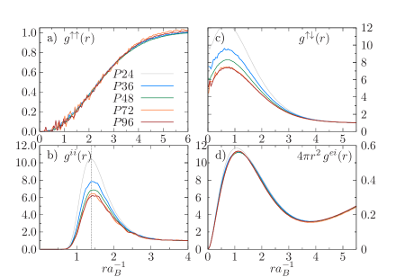
Figure 1: Dependence of the pair distribution functions on the number of factors $P$, for $T=15,640$ K, $r_{s}=7$, and the particle number $N=34$. a) PDF for same spin electrons; b) ion PDF; c) PDF for electrons with anti-parallel spins; d) electron-ion PDF. The presence of neutral bound complexes $H,H_{2}$ and molecular ions $H_{2}^{+}$ can be identified from the broad peaks in $g^{ii}(r)$ for ion-ion distances, $1.1a_{B}\leq r\leq 2.2a_{B}$, and $g^{\uparrow\downarrow}(r)$. The fraction of molecules, contributing to the peak height in $g^{ii}(r)$ (the vertical dotted line denotes the bond length $l_{B}=1.4a_{B}$ in $H_{2}$), however, is strongly overestimated for the cases with only few propagators $P=24(36)$. Full convergence is achieved only at $P=72(96)$. The atom fraction (related to the peak height in panel d) has only a weak $P$-dependence.

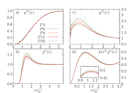
Figure 2: Same as Fig. 1, but for $T=31,250$ K and $r_{s}=5$. The molecular fraction is strongly overestimated for $P=4$, and convergence is achieved at $P=12(16)$, [cf. Fig. b)]. As for lower temperatures, the peak height in $4\pi r^{2}g^{ei}$ in panel d) exhibits only a weak $P$-dependence.

First, we address the $P$-convergence of the PDF at $T=15,640$K, in Fig. 1, and $T=31,250$K, in Fig. 2. The four panels clearly demonstrate how sensitive the inter-particle correlations are to the choice of $P$. In PIMC simulations higher $P$-values are, in general, required to accurately include the effects of three-body and higher-order correlations. This is obviously the case for the attractive Coulomb interaction experienced by the electrons within an atom or a molecule what explains the significantly slower convergence of both $g^{\uparrow\downarrow}(r)$ and $g^{ii}(r)$, compared to $g^{\uparrow\uparrow}(r)$ and $g^{ei}(r)$.

The increase of $g^{\uparrow\downarrow}>1$, below $r=1a_{B}$ (panels b) indicates the formation of molecules, which are also clearly observed as attractive correlations between pairs of atoms, with a broad peak in $g^{ii}(r)$ at $r\sim 1.4a_{B}$ (panels c). Note, that the peak amplitude becomes strongly suppressed at $P>48(15kK)$, and $P>12$ (31kK). Convergence is reached only for $P\geq 72$, for $15$kK and $P\geq 16$, for $31$kK (the corresponding lines agree within the statistical errors). The same trend is observed in $g^{\uparrow\downarrow}(r)$ as well. By using too low $P$-values [e.g. $P=24$, for 15kK, and $P=8$, for 31kK] the attractive interaction within the bound complexes ($H_{2},H_{2}^{+}$) is significantly overestimated. First, this has a strong effect on the plasma composition at low temperatures (see the cluster analysis in Sec. IV.4), and, second, influences all thermodynamic functions including the EOS.

In contrast, significantly lower $P$-values are sufficient to describe the correlations between the spin-like electrons (panels a). These electrons do not participate in molecule formation and, their short-range Coulomb repulsion is enhanced by Pauli blocking which is taken into account by the anti-symmetrization of the many-body density matrix employing Slater determinants (40). A similar effect was observed for the UEG Groth et al. (2016b); Filinov et al. (2021), where only few (fourth-order) propagators [$P\sim 2\dots 3$] were found to be sufficient even for temperatures below the Fermi temperature, $0.5\leq\theta$.

Finally, we analyze the electron-ion PDF (panels d). It does show some weak $P$-dependence, but only in the range $0.5a_{B}\leq r\leq 1.5a_{B}$. This behavior is physically reasonable: at short distances ($r\leq 0.5a_{B}$) pairwise e-i correlations dominate over the many-body effects, and the employed pair approximation for the $N$-body density matrix Ceperley (1995b); Militzer and Pollock (2000) becomes nearly exact. The influence of the plasma environment on the electron density within an atom becomes significant only at distances $r\gtrsim a_{B}$ where the pair-product ansatz for the $N$-body density matrix is not appropriate.

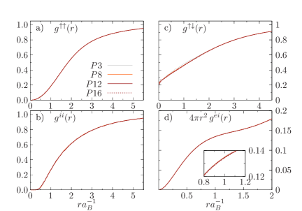
Figure 3: The PDF similar to Fig. 1 at $T=125,000$ K and $r_{s}=5$. In contrast to low temperatures ($T\leq 35,000$K), $P=3$ is completely sufficient to accurately capture the electron-electron and the electron-ion correlations.

The relative importance of many-body effects for the PDF and the influence of the number $P$ is further analyzed in Fig. 3 for a higher temperature ($T=125,000$ K) when only few bound complexes are present. For the density $r_{s}=5$ the lowest value $P=9$ is completely sufficient for accurate thermodynamic functions. Some minor effects can be resolved only in the e-i PDF (panel d) at $r\sim a_{B}$, as demonstrated in the inset. Physically, a particular choice of $P$ has an effect on the interaction between neutrals and free electrons once they approach each other to distances comparable to the effective atomic radius. This effect can be observed as an onset of formation of a local maximum in $4\pi r^{2}g^{ei}$ at $0.8\lesssim ra_{B}^{-1}\lesssim 1.2$, and this type of correlations exhibits the slowest $P$-convergence.

IV.1.2 Convergence of thermodynamic functions

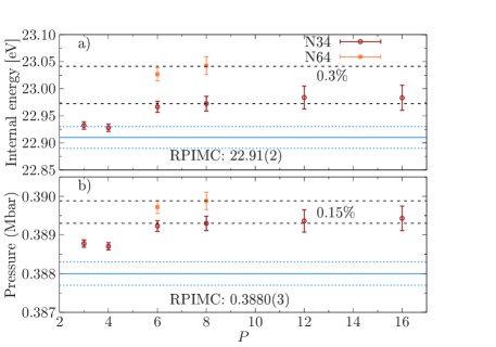
Figure 4: Convergence of (a) internal energy (per atom) and (b) pressure vs. $P$, for $r_{s}=5$ and $T=125,000$K. The extrapolation to the $P\to\infty$ limit is indicated by the dashed lines. The numbers in percent indicate the relative deviation between two system sizes $N=34$ and $N=64$. The RPIMC data Hu et al. (2011b) are shown by the solid blue line (dashed lines are the error bars).

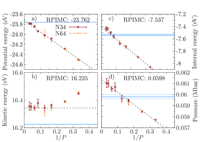
Figure 5: $1/P$-dependence of (a) kinetic energy, (b) internal energy, (c) kinetic energy , (d) pressure for $T=31,250$ K and $r_{s}=5$ and a number of factors $3\leq P\leq 32$. The extrapolation to the $P\to\infty$ limit is indicated by the dashed lines. Horizontal blue lines: RPIMC data Hu et al. (2011b).

For an accurate reconstruction of the EOS the $P$-convergence of the main thermodynamic functions has to be verified, in addition to the behavior of the PDF. We start with the simplest case of high temperature, cf. Fig. 4, when convergence of the PDF is achieved with a few factors, $P=3$, see Fig. 3. Similar conclusions can be drawn here. For $P\geq 6$, the FP-PIMC estimators for the energy and the pressure converge within the statistical error bars to the $P\rightarrow\infty$-limit. To demonstrate the finite-size effects we compare simulations for $N=34$ and $N=64$. The relative deviations in percent are cited in each panel.

A similar analysis is presented in Fig. 5, for $T=31,250$K and $r_{s}=5$. Both, the internal energy and the pressure converge to the asymptotic value, now for much larger $P$-values ($P\geq 24$). A significant increase of the statistical error bars at high $P$ is due to the decay of the average sign (16) to $\langle S\rangle\sim 0.035$ $(0.025)$, for $P=12$ $(P=16)$. Note, that the thermodynamic estimator for the potential energy $\epsilon_{p}$ (panel a) exhibits a much slower $P$-convergence compared to the kinetic energy $\epsilon_{k}$ (panel b). This can be explained by a relatively slow $1/P$-convergence of atomic and molecular fractions (see Sec. IV.1.3), and a change in plasma composition has a stronger effect on $\epsilon_{p}$. The estimated molecular fraction, see Fig. 17b, is not negligible and reaches $5\%$ for $r_{s}=5$. The results saturate only for $P=24(32)$ propagators. The simulations for a larger system size $N=64$ ($P\leq 8$) agree within the error bars.

After having established the convergence of the thermodynamic functions with $P$, we now compare the results to the RPIMC data [for details, see Sec. II.2] which are shown in Figs. 4 and 5 by the blue lines with error bars. First, for $T=125,000$K, we observe good agreement between FP-PIMC and RPIMC, where the deviations are about $0.6\%$, for the total energy and $0.5\%$, for the pressure ($N=64$), with the FP-PIMC data are being larger. The same behavior of internal energy and pressure is observed for $T=31,250$K, see the results of the $P\rightarrow\infty$ limit in Fig. 5. From panel (b), it becomes clear that the main source of discrepancy is the kinetic energy which is underestimated in RPIMC by $0.1$eV which directly influences the pressure, due to the virial relation (67). Some deviations to the RPIMC EOS become more noticeable at lower temperatures, and a systematic comparison, in a wide range of densities and temperatures, will be discussed in the following sections.

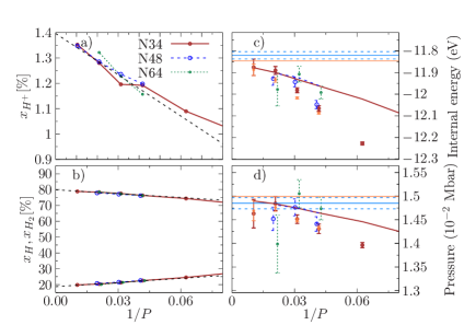
Figure 6: P-convergence of the FP-PIMC results, for $r_{s}=6$, $T=15,640$ K and $N=34$ ($P\leq 96$), $N=64$ ($P\leq 72$, see different symbols). (a) Fraction of free ions. (b) Upper (lower) curve: fraction of atoms (molecules). (c) Internal energy, and (d) pressure. Solid brown ($N=34$), dashed blue ($N=48$) and dotted green ($N=64$) lines in (c) and (d) are the HSCM model results, Eqs. (69, 68), with the $N$- and $P$-dependent fractions $\{x_{H^{+}},x_{H},x_{H_{2}}\}$ derived from the FP-PIMC data in panels (a) and (b). The extrapolation to the $P\to\infty$ limit is indicated by the horizontal (sienna) line. Horizontal blue lines in c) and d): RPIMC data Hu et al. (2011b).

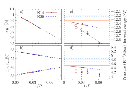
Figure 7: Same as in Fig. 6, but for $r_{s}=4$, $T=15,640$ K and $N=14,20$. Horizontal blue lines in c) and d): RPIMC data Hu et al. (2011b).

IV.1.3 Convergence of the plasma composition

Next, in Figs. 7–8 we concentrate on the low temperature case ($T=15,640$K), where the plasma is dominated by atoms and molecules. This regime was found to be the most difficult for the convergence analysis. A full $P$-convergence of all quantities cannot be achieved directly, even with a number of $P=96$ fourth-order propagators, corresponding to approximately $300$ imaginary time slices in total. The main reason is the relatively slow convergence of the ion-ion and the opposite spin electron PDFs, see Fig. 1. The peak height of both characterizes the change in the molecular (atomic) fraction and exhibits a strong $P$-dependence. As a result the bound electrons and ions contribute very differently to the kinetic and potential energy, depending on whether they belong to a molecule or to an atom. Also the dissociation equilibrium between the neutral bound complexes has a significant effect on the pressure.

Taking into account these preliminary considerations, we develop a new scheme to perform an extrapolation to the $P\rightarrow\infty$ limit. It is based on a hard-sphere chemical model (HSCM), introduced in Appendix A, based on the numerical solution of the coupled Saha equations for the hydrogen ionization–dissociation equilibrium. The corresponding thermodynamic expressions for pressure and energy of the model are defined by the equations

$$\beta p=n_{a}+n_{m}+n_{i}+\beta(p_{e}^{id}+p^{(3)}_{ex}+p_{ex}^{C}),$$ (68)

$$E=\sum\limits_{s=a,m,i,e}E_{id}^{s}+E_{ex}^{HS}+E_{ex}^{C}\,,$$ (69)

where $n_{a}$ and $n_{m}$ are the densities of atoms and molecules, $p_{e}^{id}$ is the pressure of an ideal Fermi gas, $E^{s}_{id}$ are the ideal energy contributions, and the definitions of the excess (ex) contributions are provided in Appendix A.

As the input the above equations require the species fractions $\{x_{H^{+}},x_{H},x_{H_{2}}\}$ resolved either from the HSCM or extracted from the FP-PIMC cluster analysis, $x_{i}=f_{i}(r_{s},T,P,N)$, and contain an explicit dependence on the simulation parameters. In our simulations we have accurately determined the $P$-dependence of $\{x_{H^{+}},x_{H},x_{H_{2}}\}$ of free ions, atoms and molecules, as a function of $r_{s}$, $T$, and the system size $N$. These fractions have been analyzed at three different densities corresponding to $r_{s}=6,4$ and $14$ and are presented in Figs. 6–8 (panels a, b). The deduced HSCM results for internal energy and pressure, Eqs. (69) and (68), are compared in panels c), d) with the FP-PIMC data (symbols with error bars). In each case, we observe that all fractions $x_{s}$ follow a $1/P$-scaling law, where $x_{H^{+}}$ [$x_{H},x_{H_{2}}$] changes approximately by $0.5\%$ ($1\%$), from $P=96$ to $P\rightarrow\infty$, cf. panels a) [b)]. However, before using the extrapolated values, we have to verify that finite-size effects (dependence on the particle number $N$, FSE) are not significant for the results. We have performed this analysis which revealed that FSE are negligible for $N\geq 34$ (as in Figs. 4 and 5). Therefore, the extrapolation results for the plasma composition can be considered valid, also in the thermodynamic limit. More details on the treatment of FSE are given in Sec. IV.1.4).

We now discuss the improved extrapolation procedure that exploits the chemical model, starting from the intermediate density ($r_{s}=6$, Fig. 6), where the best agreement between our HSCM-model and the FP-PIMC is observed. Indeed, the HSCM-curves reproduce the PIMC data ($N=34,48,64$) for pressure and energy [Figs. c), d)] within the statistical error bars for $P\geq 30$. Interestingly, a number $P=30$ of fourth-order propagators corresponds to an effective temperature $3\times P\times 15,640$K$\approx 1.5\cdot 10^{6}$K which is close to the value $2\cdot 10^{6}$ K that was found sufficient to accurately reproduce the properties of an isolated hydrogen molecule by Militzer et al. Militzer and Ceperley (2001b).

Next, consider a higher density corresponding to $r_{s}=4$, cf. Fig. 7. Here the degeneracy is significantly increased leading to a rapid increase of the FSP with both $P$ and $N$, and we have to restrict our FP-PIMC simulations to $N=14(20)$. This situation makes an accurate extrapolation to $P\to\infty$ and to the thermodynamic limit very complicated. Here we strongly benefit from the strongly improved convergence of the species fractions in the chemical model. In fact, the HSCM data experience a $1/P$-dependence similar to the scaling of the FP-PIMC data (see the black dashed line obtained by a linear extrapolation). Even though the slopes are different, in both cases the same $P\rightarrow\infty$ limit (shown by the solid horizontal sienna line) is approached.

Finally, for the lowest density case, $r_{s}=14$, cf. Fig. 8 a) and b), we observe some fluctuations in the fraction of bound states with the particle number for $34\leq N\leq 64$. This is related with the slow convergence of thermodynamic averages at low densities: one has to sample a significantly larger number of configurations, giving rise to an increase of the simulation time. Therefore, we choose the $N=34$ as a reference, for $r_{s}=6$ and $r_{s}=14$. However, we observe that the $1/P$-slope predicted by HSCM noticeably deviates from the $1/P$-scaling of the FP-PIMC data (dashed black line). The observed discrepancy in the energy (pressure) is about $1\%$ ($3\%$), and indicates that this method is not applicable in the present case, without substantial improvement of the HSCM.

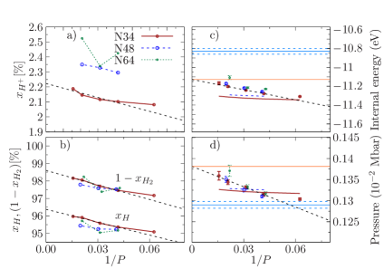
Figure 8: Same as in Fig. 6, but for $r_{s}=14$, $T=15,640$ K and $N=20,34,48,64$. The chemical model (solid brown ($N=34$) and dashed blue ($N=48$) curves) predict different $1/P$-slopes in the FP-PIMC data, therefore, we use the latter to extract the $P\to\infty$ limit (horizontal sienna line).

Finally, we compare our extrapolated results for pressure and internal energy to the RPIMC data Hu et al. (2011b) which are shown in Figs. 6–8 by the horizontal blue lines. While for $r_{s}=6$ both simulations agree within the error-bars, cf. Fig. 6, for $r_{s}=14$ and $r_{s}=4$ systematic deviations are observed. A more systematic analysis will be performed below for the pressure and energy isotherms.

IV.1.4 Finite size effects

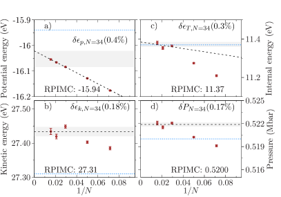
Figure 9: Convergence of the thermodynamic quantities with the system size $N=14\,,20\,,34\,,48\,,64$ for $r_{s}=4$ and $T=95\,250$ K and $P=4$. Dashed lines: linear extrapolation to the thermodynamic limit. The shaded area is the confidence interval for the mean thermodynamic value $\langle\hat{O}\rangle$: $O(\infty)-\Delta O_{N}$, for all simulations with $N\geq 34$. In parentheses we provide the relative deviation of the finite-size result $\langle O_{N=34}\rangle$ from the asymptotic value, $\delta O_{N=34}/O(\infty)$ [$\%$]. Horizontal dotted blue lines: RPIMC data Hu et al. (2011b).

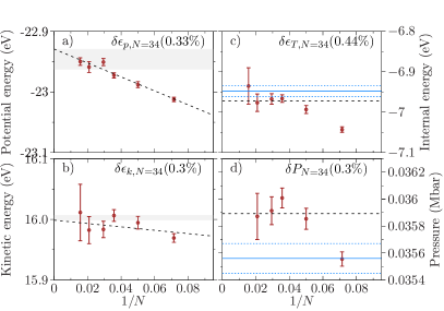
Figure 10: Same as in Fig. 9, but for $r_{s}=6$ and $T=31,250$ K. The finite-size effects, $14\leq N\leq 64$, are estimated using $P=12$. The convergent result is obtained via $1/P$-extrapolation, as explained in Fig. 5.

In this section we analyze the influence of the finite size effects (FSE). The convergence of the FP-PIMC results strongly depends on the complexity of the FSP and, therefore, in some regions of the temperature-density plane with $n\lambda^{3}\gtrsim 3$ we have to restrict the simulations to $N\leq 34$. Nevertheless, by the inclusion of periodic boundary conditions via the Ewald summation Allen and Tildesley (1987); Fraser et al. (1996) or the Yakub procedure Yakub and Ronchi (2005), the $N$-dependence of the thermodynamic observables is substantially reduced. This is illustrated below for two relevant cases: the first is that of a partially ionized plasma and the second corresponds to a situation where atoms and molecules dominate. To study the FSE we performed simulations with $N=14,20,34,48,64$ ions.

For the first case we chose $r_{s}=4$ and $T=95,250$K, where only few bound states are present. The four main thermodynamic functions are plotted in Fig. 9 and exhibit an almost linear $1/N$-scaling. The relative deviation of the reference system size ($N=34$) from the TDL in percent is indicated in each panel and provides a quantitative estimate of possible finite-size errors. This also applies to the values reported in Appendix B, including the special cases when, due to the FSP, the simulations were restricted to $N\leq 20$.

Several important conclusions can be drawn. The smallest (and the largest) FSE are observed in the kinetic $\epsilon_{k}$ (and the potential $\epsilon_{p}$) energy contributions. The kinetic energy estimator (61) has a factor $3-4$ larger statistical error compared to $\epsilon_{p}$, but it is much less influenced by the FSE than the potential energy. In particular, for $N=20$ the estimated kinetic energy deviates from the TDL by $\delta\epsilon_{k,N=20}\sim 0.2\%$, while the deviations in the potential energy reach up to $\delta\epsilon_{p,N=20}\sim 1\%$. Since the internal energy (64) and the pressure (67) contain both quantities (with different weights), the related FSE can be reduced significantly, once they are removed from the potential energy Dornheim et al. (2016b); Filinov et al. (2021).

The second case, corresponding to $T=31,250$K and $r_{s}=6$, cf. Fig. 10, exhibits very similar scaling relations. Note, that the FSE are practically absent in the kinetic energy (panel b) and pressure (panel d), even for the smallest system size $N=20$. For the lower temperature $T=15,640$K (not shown) this occurs even for $N=14$. In this regime the plasma composition is dominated by bound states (see below), and an almost ideal neutral gas behavior is expected at $r_{s}\geq 6$ with only a weak dependence on the system size.

After having analyzed the convergence of our FP-PIMC simulations with respect to $P$ and $N$ we now turn to a discussion of the thermodynamic properties.

IV.2 EOS at high temperatures and low densities: the non-degenerate case

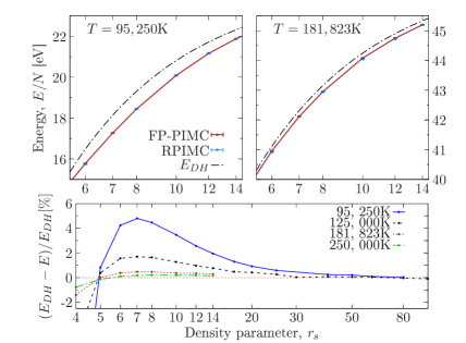
Figure 11: Upper panels: Internal energy per particle versus the density parameter, for $T=95,250$K and $181,823$K. The FP-PIMC ($N=64$) is compared to RPIMC EOS Hu et al. (2011b) and the Debye-Hückel limit (DH) (71), $E_{\text{DH}}$ (dashed-dotted line). Lower panel: Relative deviations of the FP-PIMC energy from $E_{\text{DH}}$ for four temperatures.

In this section we analyze the EOS at high temperatures, $T\geq 95,250$K, and low densities, $r_{s}\geq 5$ ($\rho_{H}\leq 2.15\cdot 10^{-2}$g/cm³), where the plasma is non-degenerate and strongly or even completely ionized. Isotherms of total energy and pressure are shown in Figs. 11 and 12 and display the expected monotonic increase with $r_{s}$. For $k_{B}T>1Ry$ (right figures), in the low-density limit, the pressure approaches the classical ideal gas result, $p_{cl}=(n_{e}+n_{i})k_{B}T$, and the energy, $2\frac{3}{2}k_{B}T$. When the density increases, interaction effects grow, and the leading correction to the ideal gas behavior is given by the Debye-Hückel limit (DH Debye and Hückel (1923)):

$$\beta p_{\text{DH}}=\beta p_{\rm id}-\frac{\kappa^{3}}{24\pi},$$ (70)

$$E_{\text{DH}}=E_{\rm id}-k_{B}T\frac{\kappa^{3}}{8\pi n},$$ (71)

where the inverse Debye length, $\kappa^{2}=4\pi ne^{2}/k_{B}T$, is defined by the full density, $n=n_{i}+n_{e}$, and we introduced $\beta p_{\rm id}=n_{i}+\beta p^{\rm id}_{e}\,,E_{\rm id}=\frac{3}{2}k_{B}T+\frac{2}{3}\frac{p^{\rm id}_{e}}{n_{e}}\,,$ where $p^{\rm id}_{e}$ is the pressure of an ideal Fermi gas.

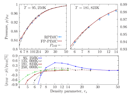
Figure 12: Same as Fig. 11, but for the pressure isotherms plotted in units of $p_{cl}=(n_{e}+n_{i})k_{B}T$.

Extending the FP-PIMC simulations to low densities, $r_{s}=100$, we can establish the validity range of the DH limit: it is generally very accurate for $r_{s}\gtrsim 20$ and, when the temperature increases, the density range grows towards smaller $r_{s}$, cf. lower panels of Figs. 11 and 12. In contrast, when the density increases, $r_{s}\lesssim 20$, the DH approximation underestimates the (negative) correlations in the plasma, and it entirely misses bound states.

Finally, we compare the FP-PIMC results to the RPIMC EOS Hu et al. (2011b) shown by the blue symbols in the top parts of Figs. 11 and 12. For the energy isotherms, we observe perfect agreement in the entire density range where RPIMC data are available ($r_{s}\leq 14$). At the same time, RPIMC slightly underestimates the pressure. This good agreement could be expected, as in the density range of $5\leq r_{s}\leq 14$ the electron degeneracy factor varies between $4\leq\theta\leq 61$, i.e. the electrons are non-degenerate, and the fixed-node approximation does not have a significant impact on the simulations.

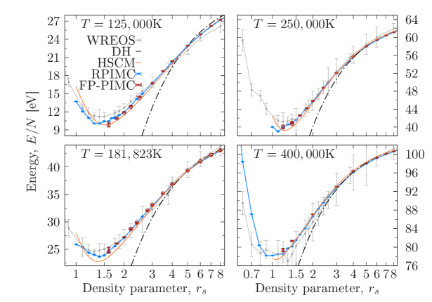
Figure 13: Isotherms of internal energy for four temperatures $T=125,000-400,000$K. Red symbols: FP-PIMC data for $N=34(64)$. Blue symbols: RPIMC, grey symbols with error bars: WREOS; dash-dotted line: Debye-Hückel limit (DH); orange lines: chemical model (“HSCM”).

IV.3 EOS at moderate and high densities: the case of degenerate electrons

We now turn to higher densities, $1.5\leq r_{s}\leq 8$, corresponding to a hydrogen mass density $5\cdot 10^{-3}\text{g/cm}^{3}\leq\rho_{H}\leq 0.80\,$g/cm³, where electron degeneracy effects become important. The results are presented in Figs. 13–15.

We start by considering the case of high temperatures, $T\geq 125,000$ K where the plasma is (almost) fully ionized. Figure 13 shows four energy isotherms and compares our FP-PIMC results to alternative models that were introduced in Sec. II.2. The overall behavior of the isotherms is well known: from the low-density limit the energy monotonically decreases, due to an increase of (negative) Coulomb correlations. Upon further density increase growth of Coulomb correlations competes with a more rapid increase of quantum kinetic energy resulting in an energy minimum around $r_{s}=1\dots 1.5$, after which the energy increases steeply. Our FP-PIMC simulations allow us to accurately determine the total energy isotherms (cf. red symbols in Fig. 13) and to come close to the energy minimum: we reach $r_{s}=1.6$, for $T=125,000$K and $r_{s}=1.2$, for $T\geq 250,000$K. For $r_{s}<1.2$ FP-PIMC simulations are not feasible due to the FSP: the electron degeneracy parameter reaches $\theta=0.53$, whereas the average sign, Eq. (16), drops below $2\cdot 10^{-3}$.

The analysis of the energy isotherms is extended to lower temperatures in Figs. 14 and 15 where we, in addition, include also the equation of state. For $T=95,250$ K our simulations are possible up to $r_{s}=2$. Interestingly, while we cannot access the energy minimum (which is around $r_{s}=1.5$), we completely resolve the pressure minimum which occurs at significantly lower densities (around $r_{s}\approx 2.5$). The same is observed for $T=62,500$ K, cf. Fig. 15, where the error bars are still reasonably small. For $T=31,250$ K we reach $r_{s}=4$ which is very close to the minimum, but at least another data point at higher density would be needed to give a conclusive answer. Thus we can provide first-principle data for the location and depth of the pressure minimum, for $T\geq 62,500$ K. Since this minimum arises from a competition of a variety of physical effects (see above) which are difficult to capture simultaneously in simpler models, our data constitute highly valuable benchmarks for other models.

Due to the limitations of the FP-PIMC simulations by the FSP, it is interesting to explore how accurate the chemical model (HSCM) is that was introduced and applied in Sec. IV.1.3, and whether it is suitable to provide an extension of the isotherms to smaller $r_{s}$. It turns out that the HSCM model (solid orange lines) is particularly well adopted to the energy isotherms and is accurate for all densities in the very broad range $r_{s}\geq 3$. Also, the HSCM model seems to qualitatively capture the behavior of the total energy around its minimum, up to $r_{s}\sim 1$, for $T\geq 125,000$ K and up to $r_{s}\sim 1.2$, for $T\leq 125,000$ K. On the other hand, the present HSCM model is much less accurate for the pressure, see left parts of Figs. 14–16.

We now turn to the comparison with the results from other models, cf. Sec. II.2. Consider first the comparison with the RPIMC results. For all FP-PIMC data shown in Figs. 13–15 we observe agreement with RPIMC, within the statistical errors.

Next, we compare to WREOS – the wide-range EOS by Wang et al. yue Wang and fang Zhang (2008). The agreement of the energies for $T\geq 125,000$ K is very reasonable within the provided error-bars but, apparently, the energy minimum is underestimated. Similar trends are observed for the EOS and for lower temperatures and become even more pronounced for temperatures $30,000\text{K}\leq T\leq 100,000$K, cf. Fig. 15. Due to the large error bars, we did not include the data for $T=95,250$ K into Fig. 14. Note that the DFT data of Ref.  Wang and Zhang (2013) for the energy contain an unknown constant. To plot the data in Fig. 15, the single molecule ground-state energy [-15.502 eV] was subtracted.

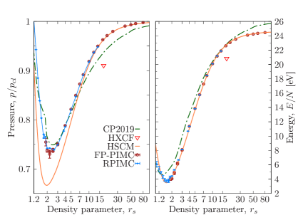
Figure 14: Isotherms of pressure (left – in units of $p_{cl}=2nk_{B}T$) and internal energy (right), for $T=95,250$K. Small red symbols: FP-PIMC data for $N=34$ and $N=20$ (at $r_{s}\leq 2$); Blue symbols: RPIMC; dash-dotted green line: CP2019; Red triangle at $r_{s}=17.53$: HXCF; Orange line: “HSCM”; cf. App. A.

Consider now the comparison to the low-density result ($r_{s}=17.53$) from the “HXCF” data by Mihaylov et al. Mihaylov et al. (2021), cf. Sec. II.2. We observe very good agreement for the energy (cf. the red triangle in Fig. 15) and a minor discrepancy in the pressure. Further, we observe the general trend that “HXCF” starts to systematically deviate from the FP-PIMC data with increasing temperature. While we find a nearly perfect agreement at $31,250$K, significant deviations appear at $95,250$K, see Fig. 14.

We now turn to the isotherms labeled “CP2019”, by Chabrier et al. Chabrier et al. (2019), cf. Sec. II.2, which are included in Figs. 14 and 15. These data extend to low densities allowing for a comparison in the range from $r_{s}\approx 3$ to $r_{s}=100$. Overall, the agreement with the FP-PIMC curves is good, with the pressure data being more accurate whereas the energies are systematically too high.

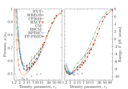
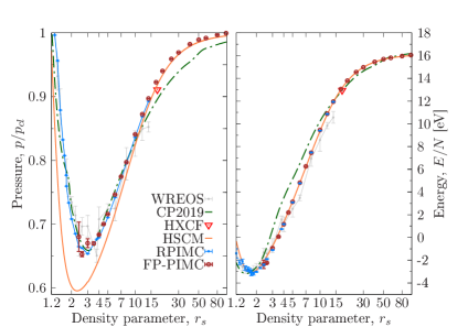
Figure 15: Same as in Fig. 14, but for $T=31,250$K (left) and $T=62,500$K (right). Open red circles: FP-PIMC data; solid blue lines with symbols: RPIMC; grey lines with error bars: WREOS; open squares: “FVT”: green dash-dotted lines: “CP2019”; red triangles at $r_{s}=17.53$: “HXCF”; orange lines: “HSCM”, grey lines in the left figure: “CM”, cf. App. A.

The fluid variational theory (FVT) by Juranek et al. Juranek et al. (2002) is included for the 31kK isotherms. We observe that, both, the total energies and pressure are substantially too low, where a comparison is possible, i.e. for $r_{s}\in[4,15]$. This is apparently caused by the contributions of unbound electrons, so the improved FVT+ model of Holst et al. Redmer et al. (2006); Holst et al. (2007) is expected to be more accurate.

IV.4 EOS in the atomic and molecular regime

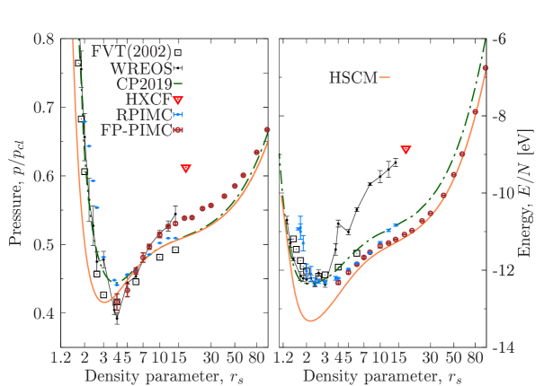
Figure 16: Same as Fig. 15, but for $T=15,640$ K. Open red circles: FP-PIMC with $P=72\dots 96$ and $N=34$, for $r_{s}\geq 4.5$ [$N=14$, for $r_{s}\geq 3.7$]; blue symbols: RPIMC; black lines with error-bars: WREOS; open squares: “FVT”; dash-dotted green lines: “CP2019”; red triangle at $r_{s}=17.53$: “HXCF”; orange lines: “HSCM”, cf. App. A.

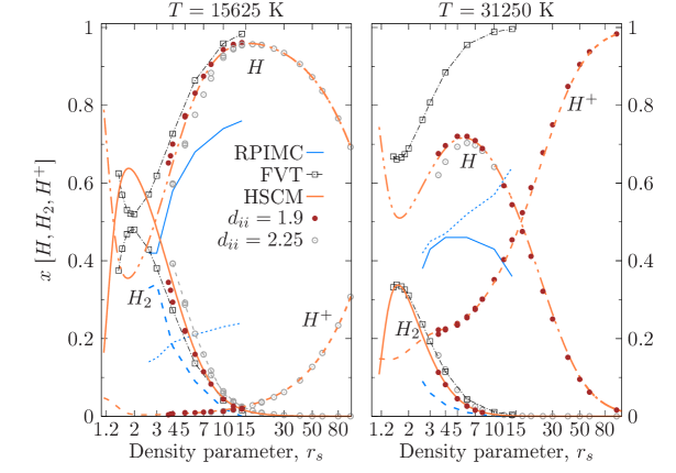
Figure 17: Fractions of molecules, atoms and free protons, for two isotherms, $T=15,640$ K (left) and $T=31,250$ K (right). FP-PIMC results are plotted for $d^{cr}_{H}=1.9a_{B}$ (brown solid dots) [$d^{cr}_{H}=2.25a_{B}$, open gray circles], for details, see text. Blue lines: RPIMC data for $d^{cr}_{H}=1.9a_{B}$; open squares: atom and molecule fractions from the FVT. Orange lines: “HSCM”, cf. Sec. A.

Now we turn to the lowest temperature in the considered range, $T=15,640$ K, where the thermodynamic functions are dominated by the contributions of neutrals. The isotherms of pressure and energy follow the trends discussed for the higher temperatures, cf. Fig. 16. Again, our simulations are severely hampered by the FSP – here we are limited to $r_{s}\geq 3.5$. We use $N=14$ ($N=20$) particles for $r_{s}\in[3.5,5]$, and $N=34$, for larger $r_{s}$. Nevertheless convergence with respect to $P$ and $N$ has been achieved, but the error bars are increasing towards lower $r_{s}$. At the same time, we observe very good agreement of our chemical model (HSCM) with the simulations, cf. the energy isotherms in Fig. 16. This indicates that the cluster analysis used to extract “fractions” of atoms and molecules from the FP-PIMC simulations is consistent (see below).

While we had observed very good agreement of RPIMC with our simulations, for $T\geq 31,250$ K before, in the present case the deviations are significantly larger, and it is interesting to analyze them in more detail. Consider first, the energy. Here we observe excellent agreement for $r_{s}\in[5,10]$. For $r_{s}=4$ the RPIMC energy is too high by about $1.5\%$ whereas for larger $r_{s}$ deviations exceed $3\%$. Let us now turn to the pressure isotherms. Here both simulations agree for $r_{s}=6$, but the FP-PIMC shows a much stronger slope in this point. Consequently, the RPIMC pressure is too high, for smaller $r_{s}$ (up to $8\%$) and too low for large $r_{s}$ (up to $5\%$).

A more detailed comparison of the FP-PIMC and RPIMC results is achieved by analyzing the microscopic configurations of the electron paths, in particular, their spatial extension. Even though the PIMC approach does not distinguish between bound and free electrons, an (artificial) distinction can be introduced via a cluster analysis, as demonstrated by Militzer et al. in Ref. Militzer and Ceperley (2001a). They introduced a critical average proton–proton separation, $d_{H}^{cr}=1.9a_{B}$, below which the configuration was “counted as a molecule”. Even though this threshold value has no direct physical meaning, it allows to better compare different PIMC simulations. This value is a reasonable estimate for the spatial extension of a molecule, if we consider the slope of the ion-ion PDF at this temperature, see Fig. 1.

We have used the same criterion for the molecules but use a modified criterion for the atoms, as explained below. The results for $T=15,625$ K and $T=31,250$ K are shown in Fig. 17. For both temperatures, we observe reasonable agreement for the molecule fractions. However, the fraction of atoms (free protons), in the FP-PIMC simulations is significantly higher (lower) than in the RPIMC data. However, since this is the case for both temperatures, whereas the thermodynamic functions, for $T=31,250$ K, are in very good agreement, this cluster analysis does not fully explain the discrepancies, see also Sec. V.

For completeness, we explain how we define the atom fraction in our FP-PIMC cluster analysis. For each ion trajectory ($\{\mathbf{r}_{p,j}=\mathbf{r}_{j}(\tau_{p}),\,0\leq\tau_{p}\leq\beta\}$) we calculate the total charge due to all electrons within a sphere of radius $R_{a}=3a_{B}$

$$\rho_{\text{net}}^{I,j}=\frac{1}{P}\sum\limits_{i=1}^{N_{e}}g_{p,i}\,\theta(\lvert\mathbf{r}_{p,i}-\mathbf{r}_{p,j}\rvert)\,,$$ (72)

averaged along the imaginary time, and

$$\theta(x)=\begin{cases}1,\lvert x\rvert\leq R_{a}\\ 0,\;\rm{else}\,.\end{cases}$$

The weighting factor $g_{p,i}$ takes into account the possibility that each electron defined by the vector $\mathbf{r}_{p,i}=\mathbf{r}_{i}(\tau_{p})$, at a given imaginary time, can be simultaneously within the radius $R_{a}$ of several ($N_{p}^{I}$) atoms. In this case its contribution on the given time slice $\tau_{p}$ is equally distributed between the nearby $N_{p}^{I}$ ions with the weight $g_{p,i}=1/N_{p}^{I}$. Following this recipe we treat an ion as “neutral” (belonging to an atom) or free particle depending on the accumulated net charge $\rho_{\text{net}}^{I,j}$, according to the criterion

$$\lvert\rho_{\text{net}}^{I,j}/e\rvert=\begin{cases}\leq 0.2,\quad\text{neutral},\quad N_{a}\to N_{a}+1\,,\\[4.30554pt] \geq 0.8,\quad\text{free ion},\quad N_{i}\to N_{i}+1\,,\end{cases}$$

where we indicated that for the cases we increase either the number of atoms or the number free ions by one.

The final fractions of free and bound ions are obtained by statistical averaging, as in the case of other observables. Finally, If two “neutrals” are found at a distance $d_{ii}\leq 1.9$ (or 2.25) $a_{B}$, they are counted as a molecule, as discussed above, and we update the number of molecules, $N_{m}\to N_{m}+1$. The corresponding particle fractions are determined by the statistical averaging similar to other thermodynamic quantities

$$\langle N_{i(a,m)}\rangle=\frac{\left\langle N_{i(a,m)}\cdot\prod\limits_{p=1}^{P}\text{Sgn}_{p}\right\rangle}{\left\langle\prod\limits_{p=1}^{P}\text{Sgn}_{p}\right\rangle}$$

where $\text{Sgn}_{p}$ is the sign of configurations due to the Slater determinants in the fermionic partition function (9). In Fig. 17 we plot the corresponding fractions of ions, atoms and molecules,

$$x[H^{+}]=\frac{\langle N_{i}\rangle}{N},\quad x[H]=\frac{\langle N_{a}\rangle}{N},\quad x[H_{2}]=\frac{2\langle N_{m}\rangle}{N}.$$

Note that the fractions of atoms and molecules that are obtained from the described cluster analysis maybe given some physical significance if the results is reasonably independent of the chosen threshold values. To this end we varied these values. As an illustration, we included results for a typical second case for the molecules, $d_{H}^{cr}=2.25a_{B}$, in Fig. 17. Obviously, the influence of the threshold is rather small which allows us to use these results in our chemical model, as well as for comparison with other approaches, such as the FVT, the results of which are also presented in Fig. 17. While the agreement with FP-PIMC is very good, for $T=15,625$ K, the model fails for $T=31,250$ K because, in the latter case, already a significant fraction of free particles ($20\%\dots 30\%$) is present.

Finally, for an additional comparison between RPIMC and FP-PIMC, in Fig. 18 we plot the kinetic and the potential energy isotherms, for three temperatures. For $T=31,250$ K and $T=62,500$ K where the total energies of RPIMC and FP-PIMC agreed within statistical errors, similar agreement is observed for the potential energy. On the other hand, we observe noticeable deviations of the kinetic energies. This shows that the kinetic energy is an observable that is very sensitive to details and, possibly errors, of the simulation procedure, whereas in the total energy deviations are reduced due to possible error compensations. This observation is confirmed for $T=15,640$ K. Here, for $r_{s}\gtrsim 6$, we observe significant deviations of both potential and kinetic energy which have opposite sign.

Finally, let us briefly summarize the comparison with the other models that are also included in Fig. 16. While the DFT-based “WREOS” data showed reasonable agreement with FP-PIMC, for $T\geq 31,250$ K, here we observe stronger deviations. For the pressure, the agreement is rather good, except for $r_{s}=4$ and $r_{s}=14$. On the other hand there are significant deviations for the internal energy which rapidly increase with $r_{s}$. Similar large deviations are observed for the “HXCF” data point for the energy at $r_{s}=17.53$. However, “HXCF” also strongly disagrees for the pressure. The EOS “CP2019” exhibits similar trends as for $T\geq 31,250$ K. Here the largest deviations (of the order of several percent) for the pressure are observed around the minimum (positive deviations) and in the range $10\lesssim r_{s}\lesssim 50$ (too low values). For the energy there appears to be an almost constant positive shift compared to FP-PIMC. Finally, the “FVT”-curve for the pressure (energy) proceeds close to the “CP2019” isotherm, for $r_{s}$-values larger than $6$ ($3$) and, hence, exhibits similar deviations from FP-PIMC.

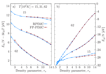
Figure 18: Isotherms of (a) kinetic energy and (b) potential energy for three temperatures indicated in the figure. FP-PIMC and RPIMC data are compared.

V Conclusions and outlook

With the upcoming new experimental facilities, in particular the colliding planar shocks platform at the NIF MacDonald et al. (2023) and the FAIR facility at GSI Darmstadt Tahir et al. (2019), high precision thermodynamic data for highly compressed matter will be available. This poses new challenges to theory and simulations. While presently a large variety of competing models and simulation approaches are being used the predictions of which often deviate significantly from one another, no hard experimental benchmarks have been available or the experimental error bars are too large for a discrimination. On the other hand, existing restricted path integral Monte Carlo simulations, which are expected to be the most accurate approach, are computationally expensive, and no independent test of their accuracy or range of applicability has been available.

In this article we have presented extensive independent fermionic PIMC simulation results for dense partially ionized hydrogen (for the present parameters these apply also to deuterium). These simulations avoid the fixed node approximation and are thus free of systematic errors. Therefore, our simulations are well capable to serve as benchmarks for RPIMC and other approaches. At high densities, the present FP-PIMC simulations are severely hampered by the fermion sign problem which restricts simulations to moderate degeneracy of the electrons – here we had to limit ourselves to temperatures above $15,000$ K and densities in the range of $r_{s}\in[2,100]$. We have presented details of our fermionic propagator PIMC approach and demonstrated in detail convergence with respect to the simulation size $N$ and the number $P$ of fourth-order propagators. The results for the equation of the state, energy contributions and pair distributions should be valuable for benchmarking and possibly improving alternative methods. Even though PIMC simulations are performed in the physical picture where no artificial distinction between “free” and “bound” electrons is necessary, we performed a cluster analysis of the spatial extension of the electrons and approximately extracted the degree of ionization and dissociation. These results are also valuable reference for other methods. In contrast to chemical models, which are hampered by an unavoidable inconsistency in the treatment of the interaction between charged particles, neutral particles and between charges and neutrals, PIMC treats all interactions and exchange effects selfconsistently. The results only depend on two parameters – the relevant average “spatial extension” of an atom and of a molecule, respectively, but the influence of this choice is small and easy to quantify, as was shown in Fig. 17.

Let us summarize our comparison with the available RPIMC data by Militzer et al. for partially ionized hydrogen. Based on earlier comparisons against first-principle CPIMC and PB-PIMC simulations for the uniform electron gas (UEG)Schoof et al. (2015b); Groth et al. (2016a); Dornheim et al. (2018a) – a much simpler system without bound states – which revealed errors on the order of $10\%$ for high densities, similar deviations could be expected. Presently, no CPIMC simulations for hydrogen are available, due to the increase of the FSP for two-component simulations. Thus, the accuracy of existing hydrogen data for high densities and strong degeneracy on the order of $\theta\lesssim 0.5$ has to be left open.

On the other hand, the present FP-PIMC simulations provide the first accurate fermionic PIMC simulations in the complementary range of $\theta\gtrsim 0.5$, translating into density parameters $r_{s}\gtrsim 4$, for $T\geq 15,640$ K and smaller values, for higher temperatures. As we have demonstrated, this is sufficient to reach the minimum of the pressure isotherms, and come close to the energy minimum. Summarizing, we conclude that the comparison for partially ionized hydrogen reveals overall very good agreement between RPIMC and FP-PIMC in the entire density range where both data sets are available, for temperatures as low as $T=31,250$ K. We interpret this as a strong independent confirmation of the extended first-principle simulations reported from the RPIMC method.

A more detailed comparison can be conducted from the EOS, Tab. 1 (see Appendix). Depending on the density-temperature range we resolve some systematic deviations, both in the pressure and energy, which are well above the statistical errors. In particular, for $T>62kK$ the deviations stay below 1%. The FP-PIMC EOS contains results for two system sizes, $N=34(64)$, and allows us to estimate the influence of FSE which are small. Therefore, the main reason for the observed discrepancies, is due to the fixed-node approximation. Consider, in particular, the lowest temperature isotherm $T=15,640$ K, cf. Fig. 16, where in the range of the minimum, deviations of up to 8% are predicted (the RPIMC data are too high). As we showed in Fig. 17, the RPIMC results significantly underestimate (overestimates) the fraction of bound complexes (free particles), in comparison to the FP-PIMC results. Also, the deviations of the RPIMC results for pressure and energy increase for lower densities, $r_{s}\gtrsim 12$, where the RPIMC data are too high by several percent. This is unexpected since there is no FSP at these parameters. Therefore, this discrepancy is, most likely, not related to the fixed node approximation but could rather reflect a sampling problem. Here, improved RPIMC data that also extend to $r_{s}=100$ would be desirable.

Finally, let us briefly summarize the results of the comparison to other methods as introduced in Sec. II.2 in the parameter range where FP-PIMC results have been reported. First, the wide range equation of state of Chabrier et al. (“CP2019”) exhibits overall a good accuracy capturing the main trends. The largest deviations for pressure and energy are on the order of several percent, in the range of the minimum of the isotherms, but there are also systematic deviations for low densities. On the other hand, the DFT-based wide-range data sets of Wang et al. (“WREOS”) and Mihaylov et al. (“HXCF”) show a different behavior. WREOS is rather accurate for $T\gtrsim 250,000$ K, but exhibits increasing discrepancies when the temperature is lowered. For the lowest temperature, $T=15,640$ K, the pressure isotherm is very accurate, however, large deviations are observed for the energy. For the comparison with HXCF we avoided parameters that are designated in Ref. Mihaylov et al. (2021) as “interpolation”. This left us with the comparison for the density $r_{s}=17.53$ where the simulation method is clear. There we observed very good agreement for $T=31,250$ K and $T=62,500$ K, but significant discrepancies for $T=95;250$ K and even larger deviations for $T=15,640$ K. Based on the comparison with a variety of DFT-MD simulations (not shown) our data should be able to discriminate between different exchange-correlation functionals. LDA-type functionals are clearly not sufficient, even though the finite temperature version (GDSMFB Groth et al. (2017)) provides some improvement. Very good agreement, at low temperatures, was observed for DFT-MD simulations with PBE functionals Wang and Zhang (2013) confirming the crucial importance of correlation effects Desjarlais (2003).

The presented comparisons are by no means exhaustive and do not pretend to be representative. The focus was on data that are available for the isotherms that were investigated in our paper (these values were selected due to existing RPIMC data), so additional errors, caused by interpolation, could be avoided. For these reasons we did not compare to other frequently used data sets including the SESAME tables or the Rostock equation of state which was reported to be close to the RPIMC results Becker et al. (2014). For more detailed comparisons, also with other methods, the reader is referred to our extensive data tables provided in the Appendix.

Due to the relative simplicity of hydrogen, first principle FP-PIMC simulations are possible that are free of systematic errors. We expect that the benchmark data presented in our paper will allow one to constrain thermodynamic data to within $1\%$, providing ample opportunities to improve alternative simulation methods as well as chemical models for the challenging conditions of warm dense matter. This will be important not only for dense hydrogen but also for the application of theoretical models and simulations to more complex materials and for reliable comparisons with existing and upcoming experiments.

Appendix A Chemical Models (HSCM)

Here we briefly summarize the chemical models “CM” and “HSCM” that have been used for comparison in some of the figures of the main text. We start with the grand potential and the ideal part of the free energy density

$$\Omega=F_{id}^{\text{HS}}+F_{id}^{C}+F^{\text{HS}}_{\text{ex}}+F^{C}_{\text{ex}}-\sum\limits_{s}\mu_{s}\rho_{s},$$

$$\beta f_{id}=\sum_{s}\rho_{s}(\ln\Lambda_{i}^{3}\rho_{i}-1)\,.$$

The free energy is decomposed into an ideal gas part, $F_{id}^{s}$, and an excess part, $F^{s}_{\text{ex}}$, related to non-ideality effects. The contribution of neutral particles (atoms/molecules, $s=\{a,m\}$), is treated on the hard sphere level (superscript “HS”), whereas the superscript “C” denotes the Coulomb contribution ($s=\{e,i\}$). Charge-neutral contributions, e.g. Schlanges et al. (1995); Redmer and Röpke (1985) are neglected.

Using the thermodynamic relations we can express the pressure, the excess chemical potential and the excess interaction energy as follows

$$p=\sum_{s}\mu_{s}\rho_{s}-(f^{s}_{id}+f^{s}_{ex}),$$

$$\mu^{a(m)}_{ex}=\frac{\partial f^{\text{HS}}_{ex}}{\partial\rho_{a(m)}},\quad\mu^{e(i)}_{ex}=\frac{\partial f^{\text{C}}_{ex}}{\partial\rho_{e(i)}}$$

$$\frac{E_{ex}^{\rm HS(C)}}{V}=f_{ex}^{\rm HS(C)}-T\,\frac{\partial f_{ex}^{\rm HS(C)}}{\partial T}\,.$$ (73)

A.1 Hard-sphere fluid model

To obtain the chemical potential and the pressure for each species “$s$” in a multi-component hard-sphere model, we follow the method proposed by Hansen-Goos et al. Hansen-Goos and Roth (2006). They introduced an expansion of the related equation of state in terms of the powers of partial densities $\rho_{s}$ and the size of all components weighted by the density contributions Rosenfeld (1989)

$$n_{0}=\sum\limits_{s}\rho_{s},\quad n_{1}=\sum\limits_{s}\rho_{s}R_{s},\;$$

$$n_{2}=\sum\limits_{s}\rho_{s}A_{s},\quad n_{3}=\sum\limits_{s}\rho_{s}V_{s}$$ (74)

where $R_{s}$, $A_{s}=4\pi R_{s}^{2}$, and $V_{s}=4/3\pi R_{s}^{3}$ are the radius, the surface area, and the volume of a sphere of species “$s$”. Systematic improvements of the original Carnahan-Starling equation of state (derived for a one-component system)

$$\frac{\beta p}{\rho}=\frac{1+\eta+\eta^{2}-\eta^{3}}{(1-\eta)^{3}}\,,$$

up to the third-order expansion in the packing fraction, $\eta=n_{3}$, have been analyzed in detail Hansen-Goos and Roth (2006). The validity of the resulting hard-sphere EOS has been justified by the accurate agreement with the simulation data.

The third order expansion has been employed in the present analysis o dissociation equilibrium in hydrogen (deuterium), where atoms and molecules have been treated as spheres of radii $\{R_{a},R_{m}\}$, with the result for the pressure

$$\beta p^{(3)}= \frac{n_{0}}{1-n_{3}}+\frac{n_{1}n_{2}(1+1/3n_{3}^{2})}{(1-n_{3})^{2}}+$$

$$\frac{n_{2}^{3}(1-2/3n_{3}+1/3n_{3}^{2})}{12\pi(1-n_{3})^{3}}\,.$$

The excess chemical potentials (A) follow as

$$\mu_{ex}^{s}=\frac{\partial f^{(3)}_{ex}}{\partial n_{3}}\,V_{s}+\frac{\partial f^{(3)}_{ex}}{\partial n_{2}}\,A_{s}+\frac{\partial f^{(3)}_{ex}}{\partial n_{1}}\,R_{s}+\frac{\partial f^{(3)}_{ex}}{\partial n_{0}}\,,$$ (75)

using the third-order $n_{3}$-expansion, $f^{(3)}_{ex}$ Hansen-Goos and Roth (2006), for the excess free energy density.

The chemical model that includes the hard sphere effects, as described above, has been called “HSCM”, in the main text, whereas the model that neglects these terms has been denoted “CM”. The deviation from the classical ideal pressure and energy (excess contribution) can be quantified by

$$\beta\Delta p_{\text{HS}}=\beta p^{(3)}-n_{0},$$

$$\Delta E_{\text{HS}}=\frac{1}{n}\left[f^{(3)}_{ex}-T\,\frac{\partial f^{(3)}_{ex}}{\partial T}\right].$$

The factor, $1/n$ (with $n=N/V$ being the total number density of ions (electrons), appears if we define $\Delta E_{\text{HS}}$ as the excess energy per ion, due to the “HS”-effect, in a system consisting of both, neutrals and free particles. Note, that the contribution of the second term in $\Delta E_{\text{HS}}$ should be accurately evaluated, as the fractions of atoms and molecules experience a noticeable variation with temperature and density. This results in a similar temperature-density dependence of the expansion variables (74) constructed from corresponding partial densities of neutrals, $\rho_{a}(r_{s},\beta)$ and $\rho_{m}(r_{s},\beta)$. Their explicit evaluation can be obtained via the solution of the non-ideal Saha equations introduced in Sec. A.2.

In the present model, we use fixed (temperature and density independent) effective radii $\{R_{a},R_{m}\}$ choosing the values $\{0.66\AA,1.32\AA\}$, obtained by the fluid variation theory of Juranek al. Juranek and Redmer (2000). We also used other radii as provided by Ref. Schlanges et al. (1995), but did observe significant changes in the considered parameter range, $r_{s}\gtrsim 3$.

A.2 Non-ideal Saha equations for the ionization–dissociation equilibrium

We impose electro-neutrality and charge conservation which leads

$$N_{i(e)}=N_{i(e)}^{\star}+N_{a}+2N_{m},\quad N_{e}=N_{i}=N\,,$$

with $N^{*}$ denoting the number of unbound electrons (ions), and $n=n_{i(e)}=N_{i(e)}/V$, the full ion (electron) density. The conditions for the dissociation-ionization equilibrium are given by

$$\mu_{m}=\mu_{a}+\mu_{a},\quad\mu_{a}=\mu_{e}+\mu_{i}\,,$$ (76)

where the chemical potential of the constituent particles are spitted into an ideal and an exchange-correlation contribution

$$\mu^{id}_{e}=\mu^{cl}_{e}+\Delta\mu_{e},$$

$$\mu_{e}+\mu_{i}=\mu^{id}_{e}+\mu^{id}_{i}+\mu_{ex}^{C},$$

$$\mu_{ex}^{C}=\frac{\partial f_{ex}^{C}}{\partial n_{e}}+\frac{\partial f_{ex}^{C}}{\partial n_{i}},$$

$$\mu_{a}=\mu^{cl}_{a}+\mu_{ex}^{a},\quad\mu_{m}=\mu^{cl}_{m}+\mu_{ex}^{m}.$$

$\mu^{a}_{ex}$ and $\mu^{m}_{ex}$ are defined in Eq. (75) by the partial derivatives of the free energy functional of a reference two-component hard-sphere system. The ideal part depends on the thermal wavelength $\lambda_{s}$, the spin degeneracy factor $g_{s}$, and the particle density $n_{s}$. For electrons and ions we take into account the “excluded volume” factor $(1-\eta)$

$$\beta\mu^{id}_{s}=\ln\left(\frac{n_{s}\lambda_{s}^{3}}{g_{s}(1-\eta)}\right).$$ (77)

The term $\Delta\mu_{e}$ in Eq. (A.2) accounts for the deviation of the ideal Fermi gas result from the classical expression (77). For the free energy density $f_{ex}^{C}$ one can employ a suitable approximation derived in  Kremp et al. (2005); Ebeling et al. (2017). In particular, we have used a quantum Debye-Hückel reduced-mass approximation where the free energy, the interaction energy and the chemical potential (due to Coulomb correlations) are expressed via Ebeling’s “ring functions”, e.g. Kremp and Schmitz (1967); Riemann et al. (1995); Ebeling (2016)

$$\beta E_{ex}^{ij}/V=-\frac{\kappa^{3}}{8\pi}G(\kappa\lambda_{ij}),$$

$$\mu_{ex}^{ij}=-\frac{1}{2}e^{2}\kappa\,G(\kappa\lambda_{ij}),$$

$$\beta f_{ex}^{ij}=-\frac{\kappa^{3}}{12\pi}R(\kappa\lambda_{ij})\,,$$

$$\beta p_{ex}^{ij}=-\frac{\kappa^{3}}{24\pi}\left[G(\kappa\lambda_{ij})+\kappa\lambda_{ij}G^{\prime}(\kappa\lambda_{ij})\right]\,,$$

which have been approximated by Padé formulas Ebeling and Richert (1982, 1985); Ebeling et al. (2017)

$$G(x)=\frac{1+0.1875x^{2}+x^{3}}{1+0.4431x+0.1963x^{2}+1.1892x^{7/2}},$$

$$R(x)=\frac{1+0.1875x^{2}+3x^{3}}{1+0.4431x+0.1963x^{2}+3.667x^{7/2}}.$$

The argument, $x=\kappa\lambda_{ij}$, includes the inverse Debye length, $\kappa^{2}=8\pi\bar{n}^{\star}\beta e^{2}$ (where $\bar{n}^{\star}$ is the re-normalized by the excluded volume effect density of free ions/electrons, see below), and $\lambda_{ij}^{2}=\hbar^{2}\beta/2\mu_{ij}$. In the reduced mass approximation we assume that the differences between the atom and ion masses are not relevant and, therefore, we set in Eqs. (73) and (A.2)

$$\mu^{i}_{ex}=\mu_{ex}^{e}=\mu_{ex}^{ei},$$

$$\mu_{ex}^{C}=\mu^{i}_{ex}+\mu_{ex}^{e}=2\mu_{ex}^{ei},$$

$$E_{ex}^{C}=E_{ex}^{ei},\quad p_{ex}^{C}=p_{ex}^{ei}.$$

Next, we consider the ionization equilibrium, which leads to the Saha equation with the non-ideality effects included via the excess chemical potential $\mu_{ex}^{I}$ of the ionization process

$$\frac{n_{a}}{n_{i}^{\star}n_{e}^{\star}}=\Lambda^{3}\,\sigma_{\text{PLB}}(\beta)\,\exp(\beta\mu_{ex}^{I}),$$ (78)

$$\mu_{ex}^{I}=\mu_{ex}^{C}+\Delta\mu_{e}-\mu^{a}_{ex}$$

where

$$\Lambda^{2}=\frac{\lambda_{e}^{2}\lambda_{i}^{2}}{\lambda_{a}^{2}}=\frac{2\pi\hbar^{2}\beta}{m_{r}},$$

$$\sigma_{\text{PLB}}(\beta)=\sum\limits_{s=1}^{\infty}s^{2}\,\left[\exp(-\beta E_{s})-1+\beta E_{s}\right]\,,$$

and $\sigma_{\text{PLB}}(\beta)$ is the regularized Planck-Brillouin-Larkin (PBL) partition function, for a discussion, see Refs. Ebeling et al. (2012); Ballenegger (2012). Now, the atom fraction can be determined from the Saha equation (78) which, however, needs to be modified to take into account the excluded volume effect: electrons and ions “cannot penetrate” neutrals, i.e. $V\rightarrow V(1-\eta)$. The packing fraction, $\eta=n_{3}$, see Eq. (74), is estimated via the number density of atoms and molecules and their radii, and re-normalizes the free electron and ion density to $\bar{n}^{\star}=n^{\star}/(1-\eta)$. Introducing the ionization fraction, $n^{\star}=\alpha_{I}n$, the mass-action law (78) can be reduced to

$$\frac{1-\alpha_{I}}{\alpha_{I}^{2}}=\frac{1}{(1-\eta)^{2}}\,K^{I}(\bar{n}^{\star},\beta,\mu_{ex}^{I}),$$

which can be solved with respect to $\alpha_{I}$ as a function of the rate constant $K^{I}$ and the excess chemical potential

$$K^{I}(\bar{n}^{\star},\beta,\mu_{ex}^{I})=\Lambda^{3}\,\sigma_{\text{PLB}}(\beta)\,\exp(\beta\mu_{ex}^{I}),$$

$$\mu^{I}_{ex}=f(\bar{n}^{\star},\beta,\alpha_{I},\alpha_{D}).$$

The second Saha equation for the dissociation equilibrium can be written in the form

$$\frac{n_{m}}{n_{a}n_{a}}=K^{D}(\beta,\mu_{ex}^{D}),$$ (79)

$$K^{D}(\beta,\mu_{ex}^{D})=\frac{g_{m}}{g_{a}g_{a}}\frac{\Lambda_{a}^{3}\Lambda_{a}^{3}}{\Lambda_{m}^{3}}Z^{\text{rot}}Z^{\text{vib}}\exp\left[\beta(D_{0}+\mu_{ex}^{D})\right],$$

$$\mu_{ex}^{D}=2\mu^{a}_{ex}-\mu^{m}_{ex}$$

where $D_{0}=4.763$eV is the dissociation energy of a $H_{2}$-molecule, and the contributions of vibrational and rotational states Mayer and Goeppert-Mayer (1948) are included via the partition functions

$$Z^{\text{rot}}\approx\frac{T}{T_{\text{rot}}}\,,$$

$$Z^{\text{vib}}\approx\left[1-\exp(-\beta T_{\text{vib}})\right]^{-1}\,,$$

where we use $T_{\text{vib}}=87.58$K and $T_{\text{rot}}=6338.2$K. For temperatures $T>1000$K, in both expression, contributions of the order $\mathcal{O}(T_{\text{rot(vib)}}/T)$ in the free energy density can be neglected. Introducing the degree of dissociation, $n_{a}=\alpha_{D}(n_{a}+n_{m})$, the mass-action law (79) becomes

$$\frac{1-\alpha_{D}}{\alpha_{D}^{2}}=K^{D}(\beta,\mu_{ex}^{D}).$$ (80)

Examples of solutions of the coupled Saha equations are included in Fig. 17. The comparison to the results of the FP-PIMC cluster analysis indicates remarkable agreement in a wide density range, $3\leq r_{s}\leq 100$, cf. Sec. IV.4 of the main text.

Appendix B Tables of FP-PIMC thermodynamic data

In this appendix we present detailed tables of our FP-PIMC simulations. In addition to the equation of state and the total energy we also present the relative deviation between our data and the RPIMC results of Militzer et al, Ref. Militzer et al. (2021). The data are converged with respect to the number $P$ of high-temperature factors and the particle number $N$. In some cases, results for several particle numbers are given to illustrate the magnitude of finite size effects. In particular, underlined numbers indicate deviations to RPIMC when we used $N=64$ particles.

Table 1: First principles FP-PIMC data for deuterium/hydrogen plasma, including pressure $p$ and internal energy $E/N$ with statistical errors given in the parantheses. The column $\Delta p/p$ denotes the relative statistical error (first number) and the deviation from RPIMC Hu et al. (2011b), i.e. $(p^{\text{RPIMC}}-p^{\text{FP-PIMC}})/p^{\text{FP-PIMC}}$), second number, and similar for $\Delta E/E$. $\theta=T/T_{F}$ is the electron degeneracy parameter. The default system size is $N=34$. For $N=64$ (if available) an extra line is added.

$T$[K]	$r_{s}$	$p$ [Mbar]	$E/N$ [eV]	$\Delta p/p\,[\%]$	$\Delta E/E\,[\%]$	$\theta$
250,000	1.2 (N20)	58.30(43)	39.98(43)	0.74(-0.85)	1.08(-0.21)	0.62
	1.4 (N20)	35.616(32)	40.69(5)	0.09(0.12)	0.13(0.75)	0.84
	1.4 (N30)	35.75(13)	40.97(20)	0.35(-0.27)	0.49(0.06)
	1.6	23.825(29)	42.62(7)	0.12(-0.40)	0.17(-0.28)	1.10
	1.8	16.7343(87)	44.19(3)	0.052	0.067	1.39
	1.8 (N64)	16.737(54)	44.27(18)	0.32	0.41
	2.0	12.2728(40)	45.852(19)	0.033(-0.59)	0.041(-0.49)	1.72
		12.314(14)	46.08(6)	0.11(-0.93)	0.14(-1.03)
	2.4	7.2001(16)	48.699(13)	0.021(0.08)	0.026(0.29)	2.47
		7.213(3)	48.86(3)	0.041(-0.096)	0.049(-0.041)
	3.0	3.76445(62)	52.087(9)	0.017(-0.30)	0.019(-0.21)	3.87
		3.76812(92)	52.202(15)	0.024(-0.40)	0.028(-0.43)
	4.0	1.62844(23)	55.7648(87)	0.014(-0.21)	0.016(-0.1)	6.88
		1.63076(31)	55.908(11)	0.019(-0.35)	0.020(-0.35)
	5.0	0.84767(12)	58.032(8)	0.013(-0.19)	0.015(-0.038)	10.75
		0.84859(15)	58.16(1)	0.018(-0.31)	0.019(-0.26)
	6.0	0.49589(7)	59.498(8)	0.014(-0.26)	0.015(-0.17)	15.47
		0.496403(95)	59.6239(12)	0.019(-0.36)	0.020(-0.37)
	7.0	0.31456(4)	60.485(9)	0.014	0.014	21.06
		0.31478(6)	60.592(12)	0.019	0.02
	8.0	0.21186(3)	61.199(9)	0.014(-0.12)	0.015(-0.03)	21.06
		0.212146(40)	61.343(12)	0.019(-0.26)	0.02(-0.26)
	10.0	0.10923(2)	62.130(9)	0.014(-0.21)	0.014(-0.06)	42.99
		0.109346(21)	62.255(12)	0.019(-0.32)	0.019(-0.26)
	12.0	0.063494(9)	62.709(9)	0.014(-0.15)	0.014(-0.06)	61.90
		0.063537(12)	62.807(12)	0.019(-0.216)	0.019(-0.217)
	14.0	0.0401099(55)	63.106(9)	0.014(-0.17)	0.014(-0.10)	84.26
		0.0401336(76)	63.196(12)	0.019(-0.23)	0.019(-0.25)
181,823	1.6 (N20)	16.59(2)	24.39(5)	0.12(0.42)	0.19(1.48)	0.80
	1.6	16.82(16)	24.98(37)	0.93(-0.92)	1.49(-0.94)
	1.8	11.679(23)	26.05(8)	0.20	0.31	1.01
	2.0	8.4965(64)	27.225(30)	0.075(-0.60)	0.11(-0.53)	1.25
	2.2	6.4233(28)	28.556(17)	0.043(-0.42)	0.061(-0.27)	1.513
	2.2 (N64)	6.447(14)	28.747(84)	0.21(-0.79)	0.29(-0.93)
	2.4	4.9830(15)	29.783(13)	0.031(-0.08)	0.042(0.20)	1.800
		4.9906(48)	29.885(39)	0.097(-0.23)	0.13(-0.15)
	2.8	3.1889(7)	32.002(9)	0.022	0.028	2.45
		3.1936(14)	32.103(18)	0.043	0.055
	3.0	2.6153(5)	33.011(8)	0.02(-0.35)	0.025(-0.31)	2.81
		2.6179(9)	33.093(14)	0.034(-0.46)	0.043(-0.55)
	3.5	1.6781(3)	35.1287(75)	0.018	0.021	3.83
		1.67937(42)	35.196(10)	0.025	0.029
	4.0	1.14179(18)	36.812(7)	0.016(-0.16)	0.018(-0.032)	5.00
		1.14300(24)	36.898(9)	0.021(-0.26)	0.025(-0.265)
	5.0	0.598717(85)	39.283(6)	0.014(-0.18)	0.016(-0.083)	7.82
		0.59918(12)	39.3579(86)	0.020(-0.26)	0.022(-0.274)
	6.0	0.352316(55)	40.955(7)	0.016(-0.17)	0.017(-0.086)	11.25
		0.352616(73)	41.033(9)	0.021(-0.26)	0.023(-0.275)
	7.0	0.224470(34)	42.115(7)	0.015	0.016	15.32
		0.224677(43)	42.200(9)	0.019	0.021
	8.0	0.151657(21)	42.954(6)	0.014(-0.10)	0.015(-0.033)	20.01
		0.151794(29)	43.0387(87)	0.019(-0.19)	0.020(-0.23)
	10.0	0.078559(11)	44.0803(67)	0.015(-0.19)	0.015(-0.09)	31.27
		0.078629(15)	44.164(9)	0.019(-0.28)	0.020(-0.28)
	12.0	0.0457687(63)	44.748(6)	0.014(-0.17)	0.014(-0.06)	45.02
		0.0458167(86)	44.8399(87)	0.019(-0.28)	0.019(-0.27)
	14.0	0.0289573(40)	45.2016(64)	0.014(-0.13)	0.014(-0.025)	61.28
		0.0289812(55)	45.2807(9)	0.019(-0.21)	0.019(-0.20)
	17.0	0.0162524(22)	45.656(6)	0.013	0.013	90.36
	20.0	0.0100110(13)	45.9447(62)	0.013	0.0135	125
	25.0	0.00514182(71)	46.2451(64)	0.014	0.014	195
	30.0	0.00298112(42)	46.4242(66)	0.014	0.014	281
	40.0	0.12607(18) $\cdot 10^{-3}$	46.6453(70)	0.0145	0.015	500
	50.0	0.646379(90) $\cdot 10^{-3}$	46.7662(66)	0.014	0.014	782
	60.0	0.374232(53) $\cdot 10^{-3}$	46.8239(66)	0.014	0.014	1125
	80.0	0.158027(22) $\cdot 10^{-3}$	46.9102(66)	0.014	0.014	2001
	100.0	0.80937(11) $\cdot 10^{-4}$	46.9505(67)	0.014	0.014	3127

$T$[K]	$r_{s}$	$p$ [Mbar]	$E/N$ [eV]	$\Delta p/p\,[\%]$	$\Delta E/E\,[\%]$	$\theta$
125,000	1.6 (N20)	10.85(17)	9.87(40)	1.58(1.06)	4.11(5.78)	0.55
	1.8 (N20)	7.52(2)	10.91(7)	0.27(-0.29)	0.64(1.81)	0.69
	2.0 (N20)	5.4316(48)	11.82(2)	0.087(-0.34)	0.19(0.74)	0.86
	2.2 (N20)	4.0810(19)	12.823(1)	0.046(0.17)	0.092(1.53)	1.04
	2.5 (N20)	2.80676(81)	14.3374(74)	0.029(-0.505)	0.052(1.42)	1.30
	2.2	4.0941(74)	12.937(46)	0.18(-0.15)	0.35(0.64)	1.04
	2.5	2.8180(20)	14.476(18)	0.069(-0.90)	0.12(0.45)	1.30
	3.0	1.6652(5)	16.7418(85)	0.032(-0.55)	0.051(-0.49)	1.93
	3.5	1.07448(24)	18.747(6)	0.023	0.032	2.63
	4.0	0.73490(14)	20.4006(54)	0.019(-0.56)	0.026(-0.54)	3.40
	5.0	0.389230(62)	22.966(5)	0.016(-0.316)	0.020(-0.246)	5.38
	6.0	0.230966(36)	24.8116(46)	0.016(-0.20)	0.018 (-0.087)	7.73
	7.0	0.148395(23)	26.2034(46)	0.015	0.0176	10.53
	8.0	0.100851(14)	27.2199(43)	0.014(-0.050)	0.016(0.00036)	13.75
	10.0	0.052688(8)	28.6154(47)	0.015(-0.091)	0.0165(0.0160)	21.5
	12.0	0.0308841(43)	29.489(4)	0.0138(-0.142)	0.0147(0.00237)	31.0
	14.0	0.0196128(27)	30.067(4)	0.0136(-0.0652)	0.0144(0.0422)	42.1
	17.0	0.0110505(15)	30.6457(42)	0.0134	0.0138	62.12
	20.0	0.682187(91) $\cdot 10^{-2}$	31.0026(4)	0.0133	0.0136	86.0
	25.0	0.351243(47) $\cdot 10^{-2}$	31.376(4)	0.0134	0.0136	134.0
	30.0	0.204159(30) $\cdot 10^{-2}$	31.632(5)	0.0145	0.0147	193
	40.0	0.86397(12) $\cdot 10^{-3}$	31.8596(44)	0.0138	0.014	343
	50.0	0.443236(59) $\cdot 10^{-3}$	31.9919(43)	0.0133	0.0134	537
	60.0	0.256795(34) $\cdot 10^{-3}$	32.0704(43)	0.0133	0.0134	773
	80.0	0.108558(15) $\cdot 10^{-3}$	32.1847(44)	0.0137	0.0137	1375
	100.0	0.556326(82) $\cdot 10^{-4}$	32.2407(48)	0.0148	0.0148	2149
95,250	2.2	2.905(33)	4.84(20)	1.135(1.69)	4.22(9.59)	0.79
	2.5	2.0060(42)	6.243(38)	0.208	0.61	1.02
	3.0	1.17896(67)	8.109(10)	0.057(-0.25)	0.13(0.38)	1.47
	3.0 (N64)	1.1856(25)	8.230(40)	0.21(-0.81)	0.48(-1.09)	1.47
	4.0	0.52179(12)	11.3647(47)	0.024(-0.34)	0.042(0.046)	2.62
		0.52180(23)	11.3797(88)	0.045(-0.345)	0.078(-0.085)	2.62
	5.0	0.278393(52)	13.851(4)	0.019(-0.14)	0.027(-0.22)	4.09
		0.278450(84)	13.8713(62)	0.030(-0.16)	0.045(-0.37)	4.09
	6.0	0.166672(27)	15.7828(34)	0.016(-0.34)	0.022(-0.27)	5.90
		0.166827(36)	15.8144(46)	0.0216(-0.435)	0.029(-0.47)	5.90
	7.0	0.107805(16)	17.2732(33)	0.015	0.019	8.02
		0.107891(22)	17.3055(45)	0.020	0.026	8.02
	8.0	0.073792(11)	18.4462(33)	0.015(-0.11)	0.018(0.02)	10.48
		0.073826(15)	18.4723(44)	0.0197(-0.16)	0.0238(-0.12)	10.48
	10.0	0.0389322(58)	20.0895(35)	0.015(-0.16)	0.017(-0.048)	16.4
		0.0389756(80)	20.1351(47)	0.020(-0.27)	0.0236(-0.274)	16.4
	12.0	0.0229801(33)	21.1608(34)	0.014(-0.044)	0.016(0.091)	23.6
		0.0230113(53)	21.2114(64)	0.023(-0.18)	0.0256(-0.148)	23.6
	14.0	0.0146659(21)	21.8805(34)	0.014(-0.176)	0.016(-0.048)	32.1
		0.0146822(30)	21.9259(48)	0.020(-0.287)	0.022(-0.255)	32.1
	17.0	0.83024(12) $\cdot 10^{-2}$	22.5957(33)	0.014	0.015	47.3
		0.83092(16) $\cdot 10^{-2}$	22.6365(46)	0.019	0.020	47.3
	20.0	0.514349(71) $\cdot 10^{-2}$	23.0538(33)	0.0137	0.014	65.5
	25.0	0.265675(37) $\cdot 10^{-2}$	23.5141(34)	0.014	0.0143	102.4
	30.0	0.155475(32) $\cdot 10^{-2}$	24.0883(50)	0.0205	0.021	147.4
	40.0	0.655798(95) $\cdot 10^{-3}$	24.0844(35)	0.014	0.0146	262.0
	50.0	0.336680(50) $\cdot 10^{-3}$	24.2311(36)	0.0148	0.0149	409.0
	60.0	0.195317(27) $\cdot 10^{-3}$	24.3396(34)	0.014	0.014	589.6
	80.0	0.825642(12) $\cdot 10^{-4}$	24.443(3)	0.014	0.014	1048
		0.826306(94) $\cdot 10^{-4}$	24.4754(28)	0.0114	0.0115	1048
	100.0	0.423114(60) $\cdot 10^{-4}$	24.4946(34)	0.014	0.014	1638

$T$[K]	$r_{s}$	$p$ [Mbar]	$E/N$ [eV]	$\Delta p/p\,[\%]$	$\Delta E/E\,[\%]$	$\theta$
75,000	3.0	0.8659(48)	2.49(8)	0.55	3.1	1.16
	4.0	0.38091(30)	5.098(11)	0.08	0.22	2.06
	5.0	0.204275(94)	7.3549(70)	0.046	0.094	3.22
	6.0	0.122951(45)	9.1967(58)	0.037	0.063	4.64
	7.0	0.080013(32)	10.7006(64)	0.040	0.055	6.32
	8.0	0.055101(18)	11.9415(56)	0.034	0.047	8.25
	10.0	0.0294190(88)	13.816(6)	0.030	0.038	12.9
	12.0	0.017534(54)	15.1083(56)	0.031	0.037	18.6
	14.0	0.0112658(37)	16.0037(62)	0.033	0.039	25.28
62,500	2.6 (N20)	1.044(12)	-2.10(12)	1.17(0.37)	5.9(-9.5)	0.726
	3.0	0.6901(71)	-0.95(11)	1.03(-2.48)	11.7(17.1)	0.967
	3.5	0.4343(15)	0.069(37)	0.34	54.	1.32
	3.5 (N64)	0.393(22)	-0.93(55)	5.62(-11.)	59.2(-179.)	1.32
	4.0	0.29689(41)	1.1610(16)	0.14(-0.64)	1.32(0.73)	1.70
		0.2966(13)	1.1579(50)	0.44(-0.55)	4.25(1.04)	1.70
	4.5	0.21366(18)	2.194(9)	0.082	0.43	2.17
		0.21529(62)	2.290(33)	0.29	1.44	2.17
	5.0	0.1592(1)	3.137(7)	0.063(-0.77)	0.23(-1.60)	2.70
		0.15961(18)	3.167(13)	0.11(-1.0)	0.41(-2.53)	2.70
	6.0	0.096076(43)	4.815(5)	0.04(-0.60)	0.11(-0.88)	3.86
		0.096196(53)	4.8309(68)	0.055(-0.72)	0.14(-1.20)	3.86
	7.0	0.062783(24)	6.2589(48)	0.037	0.076	5.27
		0.062850(36)	6.2774(72)	0.057	0.12	5.27
	8.0	0.043290(15)	7.4536(46)	0.035(-0.09)	0.062(0.31)	6.87
		0.043430(22)	7.5013(66)	0.05(-0.415)	0.088(-0.32)	6.87
	10.0	0.0233774(71)	9.450(4)	0.03(-0.54)	0.045(-0.52)	10.75
		0.02337(1)	9.4544(61)	0.044(-0.525)	0.064(-0.56)	10.75
	12.0	0.0140376(41)	10.8839(43)	0.029(-0.41)	0.040(-0.22)	15.5
		0.0140452(60)	10.8992(62)	0.043(-0.46)	0.057(-0.36)	15.5
	14.0	0.90889(27) $\cdot 10^{-2}$	11.9542(45)	0.029(-0.47)	0.038(-0.20)	21.0
		0.90993(40) $\cdot 10^{-2}$	11.9828(67)	0.044(-0.58)	0.056(-0.44)	21.0
	17.0	0.52209(15) $\cdot 10^{-2}$	13.0526(46)	0.029	0.035	31.0
	20.0	0.3267(1) $\cdot 10^{-2}$	13.7865(48)	0.030	0.035	43.0
	25.0	0.170665(61) $\cdot 10^{-2}$	14.5465(56)	0.036	0.039	67.0
		0.17071(8) $\cdot 10^{-2}$	14.5601)(73)	0.047	0.050	67.0
	30.0	0.99795(41) $\cdot 10^{-3}$	14.9682(65)	0.041	0.043	96.5
	40.0	0.42666(15) $\cdot 10^{-3}$	15.4458(56)	0.035	0.036	171
		0.42736)(19) $\cdot 10^{-3}$	15.4848(79)	0.044	0.045	171
	50.0	0.220030(68) $\cdot 10^{-3}$	15.6877(50)	0.031	0.031	268.7
		0.2202(1) $\cdot 10^{-3}$	15.7203(72)	0.045	0.046	268.7
	60.0	0.127664(38) $\cdot 10^{-3}$	15.8019(48)	0.030	0.030	386
		0.127874(57) $\cdot 10^{-3}$	15.842(7)	0.044	0.045	386
	80.0	0.54130(16) $\cdot 10^{-4}$	15.9597(48)	0.030	0.030	687
	100.0	0.277896(80) $\cdot 10^{-4}$	16.0419(47)	0.029	0.029	1074
50,000	3.0	0.5005(41)	-4.556(64)	0.82	1.41	0.77
	4.0	0.21794(81)	-2.749(30)	0.37	1.10	1.38
	5.0	0.11642(13)	-1.1855(95)	0.11	0.80	2.15
	6.0	0.070107(42)	0.1824(54)	0.060	2.95	3.09
	7.0	0.045865(22)	1.4186(44)	0.046	0.31	4.21
	8.0	0.031773(13)	2.5272(41)	0.042	0.16	5.50
	10.0	0.0172604(60)	4.4277(37)	0.035	0.083	8.60
	12.0	0.0104598(49)	5.9609(54)	0.047	0.091	12.40
	14.0	0.68375(24) $\cdot 10^{-2}$	7.1964(43)	0.035	0.06	16.85
	17.0	0.39738(12) $\cdot 10^{-2}$	8.5612(37)	0.030	0.044	24.85
	20.0	0.251274(71) $\cdot 10^{-2}$	9.5452(36)	0.028	0.038	34.40
	25.0	0.132898(42) $\cdot 10^{-2}$	10.6277(40)	0.031	0.038	53.74
	30.0	0.78366(31) $\cdot 10^{-3}$	11.2675(50)	0.039	0.044	77.4
	40.0	0.33759(14) $\cdot 10^{-3}$	11.9635(53)	0.042	0.044	137.5
	50.0	0.174537(78) $\cdot 10^{-3}$	12.2841(57)	0.045	0.046	215
	60.0	0.101562(55) $\cdot 10^{-3}$	12.4629(70)	0.054	0.056	309
	100.0	0.22157(12) $\cdot 10^{-4}$	12.7506(69)	0.053	0.054	860

$T$[K]	$r_{s}$	$p$ [Mbar]	$E/N$ [eV]	$\Delta p/p\,[\%]$	$\Delta E/E\,[\%]$	$\theta$
31,250	4.0 (N28)	0.1158(31)	-8.25(11)	2.70(-0.68)	1.40(-1.42)	0.86
	5.0	0.0610(4)	-7.451(30)	0.65(-1.9)	0.40(-1.11)	1.34
	6.0	0.03624(23)	-6.928(29)	0.63(-1.87)	0.41(0.28)	1.93
	7.0	0.023019(79)	-6.454(16)	0.34	0.247	2.63
	8.0	0.015877(42)	-5.892(13)	0.26(-0.48)	0.21(-0.55)	3.44
	10.0	0.85724(71) $\cdot 10^{-2}$	-4.8223(42)	0.083(-1.43)	0.088(0.39)	5.37
	12.0	0.51871(36) $\cdot 10^{-2}$	-3.8193(37)	0.069(-1.58)	0.098(0.019)	7.74
	14.0	0.33920(22) $\cdot 10^{-2}$	-2.8807(37)	0.065(-0.82)	0.13(-0.47)	10.53
	17.0	0.19977(11) $\cdot 10^{-2}$	-1.5625(34)	0.055	0.22	15.5
	20.0	0.128679(67) $\cdot 10^{-2}$	-0.3531(35)	0.052	0.99	21.5
	25.0	0.70367(34) $\cdot 10^{-3}$	1.3719(36)	0.048	0.26	33.6
	30.0	0.42727(19)$\cdot 10^{-3}$	2.7425(35)	0.045	0.13	48.4
	40.0	0.1934(1) $\cdot 10^{-3}$	4.7058(41)	0.051	0.086	86.
	50.0	0.103092(56) $\cdot 10^{-3}$	5.86616	0.054	0.073	134.4
	60.0	0.610953(35) $\cdot 10^{-4}$	6.5628(46)	0.058	0.067	344.
	100.0	0.136866(93) $\cdot 10^{-4}$	7.6035(54)	0.068	0.072	536.
15,625	4.0	0.0452(13)	-12.319(47)	2.84(6.0)	0.38(-0.89)	0.43
	$4.0$(N14)	0.0430(13)	-12.47(5)	3.(11.)	0.4(-2.0)	0.43
	5.0	0.02409(52)	-12.057(38)	2.17(5.3)	0.32(-0.72)	0.67
	6.0	0.01484(14)	-11.846(18)	0.97(0.46)	0.15(-0.22)	0.967
	7.0	0.974(14) $\cdot 10^{-2}$	-11.669(28)	1.44	0.24	1.32
	8.0	0.6743(50) $\cdot 10^{-2}$	-11.535(15)	0.74(-2.27)	0.13(0.126)	1.72
	10.0	0.3572(27) $\cdot 10^{-2}$	-11.370(51)	0.75(-2.29)	0.44(-0.79)	2.69
	12.0	0.21171(98) $\cdot 10^{-2}$	-11.2975(98)	0.465(-3.26)	0.087(-2.90)	3.87
	14.0	0.13437(54) $\cdot 10^{-2}$	-11.2028(86)	0.40(-4.0)	0.077(-3.33)	5.27
	17.0	0.7617(18) $\cdot 10^{-3}$	-11.0754(5)	0.25	0.048	7.76
	20.0	0.4685(11) $\cdot 10^{-3}$	-10.9734(5)	0.23	0.045	10.75
	25.0	0.24568(53) $\cdot 10^{-3}$	-10.724(5)	0.22	0.045	16.8
	30.0	0.14335(27) $\cdot 10^{-3}$	-10.526(4)	0.19	0.042	24.2
	40.0	0.6195(12) $\cdot 10^{-4}$	-10.062(5)	0.20	0.048	43.0
	50.0	0.32544(58) $\cdot 10^{-4}$	-9.527(4)	0.18	0.046	67.2
	60.0	0.19336(35) $\cdot 10^{-4}$	-8.9906(45)	0.18	0.05	96.7
	80.0	0.8611(11) $\cdot 10^{-5}$	-7.8957(36)	0.13	0.045	172.
	100.0	0.46378(58) $\cdot 10^{-5}$	-6.7590(36)	0.125	0.053	268.

References

- Graziani et al. (2014) F. Graziani, M. P. Desjarlais, R. Redmer, and S. B. Trickey, Frontiers and Challenges in Warm Dense Matter (Springer, 2014).
- Fortov (2016) V. E. Fortov, Extreme States of Matter (High Energy Density Physics, Second Edition) (Springer, Heidelberg, 2016).
- Moldabekov et al. (2018) Zh. A. Moldabekov, S. Groth, T. Dornheim, H. Kählert, M. Bonitz, and T. S. Ramazanov, “Structural characteristics of strongly coupled ions in a dense quantum plasma,” Phys. Rev. E 98, 023207 (2018).
- Dornheim et al. (2018a) Tobias Dornheim, Simon Groth, and Michael Bonitz, “The uniform electron gas at warm dense matter conditions,” Phys. Rep. 744, 1 – 86 (2018a).
- Saumon et al. (1992) D. Saumon, W. B. Hubbard, G. Chabrier, and H. M. van Horn, “The role of the molecular-metallic transition of hydrogen in the evolution of Jupiter, Saturn, and brown dwarfs,” Astrophys. J. 391, 827–831 (1992).
- Chabrier (1993) Gilles Chabrier, “Quantum effects in dense Coulombic matter - Application to the cooling of white dwarfs,” Astrophys. J. 414, 695 (1993).
- Chabrier et al. (2000) G. Chabrier, P. Brassard, G. Fontaine, and D. Saumon, “Cooling Sequences and Color-Magnitude Diagrams for Cool White Dwarfs with Hydrogen Atmospheres,” Astrophys. J. 543, 216 (2000).
- Schlanges et al. (1995) M. Schlanges, M. Bonitz, and A. Tschttschjan, “Plasma phase transition in fluid hydrogen-helium mixtures,” Contributions to Plasma Physics 35, 109–125 (1995).
- Bezkrovniy et al. (2004) V. Bezkrovniy, V. S. Filinov, D. Kremp, M. Bonitz, M. Schlanges, W. D. Kraeft, P. R. Levashov, and V. E. Fortov, “Monte Carlo results for the hydrogen Hugoniot,” Phys. Rev. E 70, 057401 (2004).
- Vorberger et al. (2007) J. Vorberger, I. Tamblyn, B. Militzer, and S. A. Bonev, “Hydrogen-helium mixtures in the interiors of giant planets,” Phys. Rev. B 75, 024206 (2007).
- Militzer et al. (2008) B. Militzer, W. B. Hubbard, J. Vorberger, I. Tamblyn, and S. A. Bonev, “A Massive Core in Jupiter Predicted from First-Principles Simulations,” Astrophys. J. Lett. 688, L45 (2008).
- Redmer et al. (2011) Ronald Redmer, Thomas R. Mattsson, Nadine Nettelmann, and Martin French, “The phase diagram of water and the magnetic fields of uranus and neptune,” Icarus 211, 798 – 803 (2011).
- Nettelmann et al. (2013) Nadine Nettelmann, Robert Püstow, and Ronald Redmer, “Saturn layered structure and homogeneous evolution models with different EOSs,” Icarus 225, 548–557 (2013).
- Haensel et al. (2006) P. Haensel, A. Y. Potekhin, and D.G. Yakovlev, Neutron Stars 1: Equation of State and Structure (New York: Springer, 2006).
- Daligault and Gupta (2009) J. Daligault and S. Gupta, “Electron-Ion Scattering in Dense Multi-Component Plasmas: Application to the Outer Crust of an Accreting Neutron Star,” Astrophys. J. 703, 994 (2009).
- Nora et al. (2015) R. Nora, W. Theobald, R. Betti, F.J. Marshall, D.T. Michel, W. Seka, B. Yaakobi, M. Lafon, C. Stoeckl, J. Delettrez, A.A. Solodov, A. Casner, C. Reverdin, X. Ribeyre, A. Vallet, J. Peebles, F.N. Beg, and M.S. Wei, “Gigabar Spherical Shock Generation on the OMEGA Laser,” Phys. Rev. Lett. 114, 045001 (2015).
- Matzen et al. (2005) M. Keith Matzen, M. A. Sweeney, R. G. Adams, J. R. Asay, J. E. Bailey, G. R. Bennett, D. E. Bliss, D. D. Bloomquist, T. A. Brunner, R. B. Campbell, G. A. Chandler, C. A. Coverdale, M. E. Cuneo, J.-P. Davis, C. Deeney, M. P. Desjarlais, G. L. Donovan, C. J. Garasi, T. A. Haill, C. A. Hall, D. L. Hanson, M. J. Hurst, B. Jones, M. D. Knudson, R. J. Leeper, R. W. Lemke, M. G. Mazarakis, D. H. McDaniel, T. A. Mehlhorn, T. J. Nash, C. L. Olson, J. L. Porter, P. K. Rambo, S. E. Rosenthal, G. A. Rochau, L. E. Ruggles, C. L. Ruiz, T. W. L. Sanford, J. F. Seamen, D. B. Sinars, S. A. Slutz, I. C. Smith, K. W. Struve, W. A. Stygar, R. A. Vesey, E. A. Weinbrecht, D. F. Wenger, and E. P. Yu, “Pulsed-power-driven high energy density phys. and inertial confinement fusion research,” Phys. Plasmas 12, 055503 (2005).
- Knudson et al. (2015) M. D. Knudson, M. P. Desjarlais, A. Becker, R. W. Lemke, K. R. Cochrane, M. E. Savage, D. E. Bliss, T. R. Mattsson, and R. Redmer, “Direct observation of an abrupt insulator-to-metal transition in dense liquid deuterium,” Science 348, 1455–1460 (2015).
- Ren et al. (2018) J. Ren, C. Maurer, P. Katrik, P.M. Lang, A.A. Golubev, V. Mintsev, Y. Zhao, and D.H.H. Hoffmann, “Accelerator-driven high-energy-density physics: Status and chances,” Contrib. Plasma Phys. 58, 82–92 (2018).
- Tahir et al. (2019) Naeem A. Tahir, Paul Neumayer, Alexander Shutov, Antonio R. Piriz, Igor V. Lomonosov, Vincent Bagnoud, Sofia A. Piriz, and Claude Deutsch, “Equation-of-state studies of high-energy-density matter using intense ion beams at the facility for antiprotons and ion research,” Contrib. Plasma Phys. 59, e201800143 (2019).
- Moses et al. (2009) E. I. Moses, R. N. Boyd, B. A. Remington, C. J. Keane, and R. Al-Ayat, “The National Ignition Facility: Ushering in a new age for high energy density science,” Phys. Plasmas 16, 041006 (2009).
- Hurricane et al. (2016) O. A. Hurricane, D. A. Callahan, D. T. Casey, E. L. Dewald, T. R. Dittrich, T. Döppner, S. Haan, D. E. Hinkel, L. F. Berzak Hopkins, O. Jones, A. L. Kritcher, S. Le Pape, T. Ma, A. G. MacPhee, J. L. Milovich, J. Moody, A. Pak, H.-S. Park, P. K. Patel, J. E. Ralph, H. F. Robey, J. S. Ross, J. D. Salmonson, B. K. Spears, P. T. Springer, R. Tommasini, F. Albert, L. R. Benedetti, R. Bionta, E. Bond, D. K. Bradley, J. Caggiano, P. M. Celliers, C. Cerjan, J. A. Church, R. Dylla-Spears, D. Edgell, M. J. Edwards, D. Fittinghoff, M. A. Barrios Garcia, A. Hamza, R. Hatarik, H. Herrmann, M. Hohenberger, D. Hoover, J. L. Kline, G. Kyrala, B. Kozioziemski, G. Grim, J. E. Field, J. Frenje, N. Izumi, M. Gatu Johnson, S. F. Khan, J. Knauer, T. Kohut, O. Landen, F. Merrill, P. Michel, A. Moore, S. R. Nagel, A. Nikroo, T. Parham, R. R. Rygg, D. Sayre, M. Schneider, D. Shaughnessy, D. Strozzi, R. P. J. Town, D. Turnbull, P. Volegov, A. Wan, K. Widmann, C. Wilde, and C. Yeamans, “Inertially confined fusion plasmas dominated by alpha-particle self-heating,” Nat. Phys. 12, 800–806 (2016).
- Abu-Shawareb (2022) H. Abu-Shawareb, “Lawson criterion for ignition exceeded in an inertial fusion experiment,” Phys. Rev. Lett. 129, 075001 (2022).
- Zylstra (2022) A.B. Zylstra, “Experimental achievement and signatures of ignition at the national ignition facility,” Phys. Rev. E 106, 025202 (2022).
- Igumenshchev et al. (2023) I. V. Igumenshchev, W. Theobald, C. Stoeckl, R. C. Shah, D. T. Bishel, V. N. Goncharov, M. J. Bonino, E. M. Campbell, L. Ceurvorst, D. A. Chin, T. J. B. Collins, S. Fess, D. R. Harding, S. Sampat, N. R. Shaffer, A. Shvydky, E. A. Smith, W. T. Trickey, L. J. Waxer, A. Colaïtis, R. Liotard, P. J. Adrian, S. Atzeni, F. Barbato, L. Savino, N. Alfonso, A. Haid, and Mi Do, “Proof-of-principle experiment on the dynamic shell formation for inertial confinement fusion,” Phys. Rev. Lett. 131, 015102 (2023).
- Dornheim et al. (2018b) T. Dornheim, S. Groth, J. Vorberger, and M. Bonitz, “Ab initio Path Integral Monte Carlo Results for the Dynamic Structure Factor of Correlated Electrons: From the Electron Liquid to Warm Dense Matter,” Phys. Rev. Lett. 121, 255001 (2018b).
- Dornheim et al. (2022) Tobias Dornheim, Zhandos Moldabekov, Jan Vorberger, Hanno Kählert, and Michael Bonitz, “Electronic pair alignment and roton feature in the warm dense electron gas,” Communications Physics 5, 304 (2022).
- Hamann et al. (2023) Paul Hamann, Linda Kordts, Alexey Filinov, Michael Bonitz, Tobias Dornheim, and Jan Vorberger, “Prediction of a roton-type feature in warm dense hydrogen,” Phys. Rev. Res. 5, 033039 (2023).
- MacDonald et al. (2023) M. J. MacDonald, C. A. Di Stefano, T. Döppner, L. B. Fletcher, K. A. Flippo, D. Kalantar, E. C. Merritt, S. J. Ali, P. M. Celliers, R. Heredia, S. Vonhof, G. W. Collins, J. A. Gaffney, D. O. Gericke, S. H. Glenzer, D. Kraus, A. M. Saunders, D. W. Schmidt, C. T. Wilson, R. Zacharias, and R. W. Falcone, “The colliding planar shocks platform to study warm dense matter at the National Ignition Facility,” Physics of Plasmas 30, 062701 (2023).
- Ebeling and Richert (1985) W. Ebeling and W. Richert, “Plasma phase transition in hydrogen,” Physics Letters A 108, 80 – 82 (1985).
- Trigger et al. (2003) S. A. Trigger, W. Ebeling, V. S. Filinov, V. E. Fortov, and M. Bonitz, “Internal energy of high-density hydrogen: Analytic approximations compared with path integral Monte Carlo calculations,” Journal of Experimental and Theoretical Physics 96, 465–479 (2003).
- Juranek et al. (2002) Hauke Juranek, Ronald Redmer, and Yaakov Rosenfeld, “Fluid variational theory for pressure dissociation in dense hydrogen: Multicomponent reference system and nonadditivity effects,” The Journal of Chemical Physics 117, 1768–1774 (2002), https://doi.org/10.1063/1.1486210 .
- Filinov et al. (2004) A. V. Filinov, V. O. Golubnychiy, M. Bonitz, W. Ebeling, and J. W. Dufty, “Temperature-dependent quantum pair potentials and their application to dense partially ionized hydrogen plasmas,” Phys. Rev. E 70, 046411 (2004).
- Su and Goddard (2007) Julius T. Su and William A. Goddard, “Excited electron dynamics modeling of warm dense matter,” Phys. Rev. Lett. 99, 185003 (2007).
- Ma et al. (2019) Qian Ma, Jiayu Dai, Dongdong Kang, M. S. Murillo, Yong Hou, Zengxiu Zhao, and Jianmin Yuan, “Extremely low electron-ion temperature relaxation rates in warm dense hydrogen: Interplay between quantum electrons and coupled ions,” Phys. Rev. Lett. 122, 015001 (2019).
- Filinov et al. (2002) V. Filinov, P. Thomas, I. Varga, T. Meier, M. Bonitz, V. Fortov, and S. W. Koch, “Interacting electrons in a one-dimensional random array of scatterers: A quantum dynamics and Monte Carlo study,” Phys. Rev. B 65, 165124 (2002).
- Knaup et al. (2002) M. Knaup, P.-G. Reinhard, C. Toepffer, and G. Zwicknagel, “Wave packet molecular dynamics simulations of hydrogen at mbar pressures,” Computer Physics Communications 147, 202 – 204 (2002), proceedings of the Europhysics Conference on Computational Physics Computational Modeling and Simulation of Complex Systems.
- Sjostrom and Daligault (2014) Travis Sjostrom and Jérôme Daligault, “Fast and accurate quantum molecular dynamics of dense plasmas across temperature regimes,” Phys. Rev. Lett. 113, 155006 (2014).
- Dai et al. (2010) Jiayu Dai, Yong Hou, and Jianmin Yuan, “Unified first principles description from warm dense matter to ideal ionized gas plasma: Electron-ion collisions induced friction,” Phys. Rev. Lett. 104, 245001 (2010).
- Kang and Dai (2018) Dongdong Kang and Jiayu Dai, “Dynamic electron–ion collisions and nuclear quantum effects in quantum simulation of warm dense matter,” Journal of Physics: Condensed Matter 30, 073002 (2018).
- Collins et al. (1995) L. Collins, I. Kwon, J. Kress, N. Troullier, and D. Lynch, “Quantum molecular dynamics simulations of hot, dense hydrogen,” Phys. Rev. E 52, 6202–6219 (1995).
- Plagemann et al. (2012) K-U Plagemann, P Sperling, R Thiele, M P Desjarlais, C Fortmann, T Döppner, H J Lee, S H Glenzer, and R Redmer, “Dynamic structure factor in warm dense beryllium,” New Journal of Physics 14, 055020 (2012).
- Witte et al. (2017) B. B. L. Witte, L. B. Fletcher, E. Galtier, E. Gamboa, H. J. Lee, U. Zastrau, R. Redmer, S. H. Glenzer, and P. Sperling, “Warm dense matter demonstrating non-drude conductivity from observations of nonlinear plasmon damping,” Phys. Rev. Lett. 118, 225001 (2017).
- Karasiev et al. (2014) Valentin V. Karasiev, Travis Sjostrom, and S.B. Trickey, “Finite-temperature orbital-free DFT molecular dynamics: Coupling Profess and Quantum Espresso,” Computer Physics Communications 185, 3240 – 3249 (2014).
- Sun et al. (2017) H.Y. Sun, Dongdong Kang, Yong Hou, and J.Y. Dai, “Transport properties of warm and hot dense iron from orbital free and corrected Yukawa potential molecular dynamics,” Matter and Radiation at Extremes 2, 287–295 (2017).
- Baczewski et al. (2016) A. D. Baczewski, L. Shulenburger, M. P. Desjarlais, S. B. Hansen, and R. J. Magyar, “X-ray Thomson Scattering in Warm Dense Matter without the Chihara Decomposition,” Phys. Rev. Lett. 116, 115004 (2016).
- Militzer and Ceperley (2000) B. Militzer and D. M. Ceperley, “Path Integral Monte Carlo Calculation of the Deuterium Hugoniot,” Phys. Rev. Lett. 85, 1890–1893 (2000).
- Militzer and Ceperley (2001a) B. Militzer and D. M. Ceperley, “Path integral monte carlo simulation of the low-density hydrogen plasma,” Phys. Rev. E 63, 066404 (2001a).
- V.S. Filinov (2000) V.E. Fortov V.S. Filinov, M. Bonitz, “High density phenomena in hydrogen plasma,” JETP Lett. 72, 244 (2000).
- Filinov et al. (2000) V.S. Filinov, V.E. Fortov, M. Bonitz, and D. Kremp, “Pair distribution functions of dense partially ionized hydrogen,” Phys. Lett. A 274, 228 – 235 (2000).
- Filinov et al. (2001a) V S Filinov, M Bonitz, W Ebeling, and V E Fortov, “Thermodynamics of hot dense H-plasmas: path integral Monte Carlo simulations and analytical approximations,” Plasma Phys. Control. Fusion 43, 743 (2001a).
- Filinov et al. (2001b) V.S. Filinov, M. Bonitz, D. Kremp, W.‐D. Kraeft, W. Ebeling, P.R. Levashov, and V.E. Fortov, “Path Integral Simulations of the Thermodynamic Properties of Quantum Dense Plasma,” Contrib. Plasma Phys. 41, 135–138 (2001b).
- Troyer and Wiese (2005) Matthias Troyer and Uwe-Jens Wiese, “Computational complexity and fundamental limitations to fermionic quantum monte carlo simulations,” Phys. Rev. Lett. 94, 170201 (2005).
- Dornheim (2021) Tobias Dornheim, “Fermion sign problem in path integral monte carlo simulations: grand-canonical ensemble,” Journal of Physics A: Mathematical and Theoretical 54, 335001 (2021).
- Ceperley (1991) D. M. Ceperley, “Fermion nodes,” Journal of Statistical Physics 63, 1237–1267 (1991).
- Ceperley (1996a) D.M. Ceperley, “Path integral monte carlo methods for fermions,” in Monte Carlo and Molecular Dynamics of Condensed Matter Systems, edited by K. Binder and G. Ciccotti (Italian Physical Society, Bologna, 1996).
- Hu et al. (2010) S. X. Hu, B. Militzer, V. N. Goncharov, and S. Skupsky, “Strong coupling and degeneracy effects in inertial confinement fusion implosions,” Phys. Rev. Lett. 104, 235003 (2010).
- Hu et al. (2011a) S. X. Hu, B. Militzer, V. N. Goncharov, and S. Skupsky, “First-principles equation-of-state table of deuterium for inertial confinement fusion applications,” Phys. Rev. B 84, 224109 (2011a).
- Militzer and Driver (2015) Burkhard Militzer and Kevin P. Driver, “Development of path integral monte carlo simulations with localized nodal surfaces for second-row elements,” Phys. Rev. Lett. 115, 176403 (2015).
- Filinov (2001) Vladimir Filinov, “Cluster expansion for ideal fermi systems in the ‘fixed-node approximation’,” Journal of Physics A: Mathematical and General 34, 1665 (2001).
- Filinov (2014) V. S. Filinov, “Analytical contradictions of the fixed-node density matrix,” High Temperature 52, 615–620 (2014).
- Militzer and Pollock (2000) Burkhard Militzer and E. L. Pollock, “Variational density matrix method for warm, condensed matter: Application to dense hydrogen,” Phys. Rev. E 61, 3470–3482 (2000).
- Militzer et al. (2021) Burkhard Militzer, Felipe González-Cataldo, Shuai Zhang, Kevin P. Driver, and Fran çois Soubiran, “First-principles equation of state database for warm dense matter computation,” Phys. Rev. E 103, 013203 (2021).
- Schoof et al. (2011) T. Schoof, M. Bonitz, A. Filinov, D. Hochstuhl, and J.W. Dufty, “Configuration path integral Monte Carlo,” Contrib. Plasma Phys. 84, 687–697 (2011).
- Schoof et al. (2015a) T. Schoof, S. Groth, and M. Bonitz, “Towards ab initio thermodynamics of the electron gas at strong degeneracy,” Contrib. Plasma Phys. 55, 136–143 (2015a).
- Dornheim et al. (2015) Tobias Dornheim, Simon Groth, Alexey Filinov, and Michael Bonitz, “Permutation blocking path integral Monte Carlo: a highly efficient approach to the simulation of strongly degenerate non-ideal fermions,” New J. Phys. 17, 073017 (2015).
- Dornheim et al. (2016a) T. Dornheim, S. Groth, T. Schoof, C. Hann, and M. Bonitz, “Ab initio quantum Monte Carlo simulations of the uniform electron gas without fixed nodes: The unpolarized case,” Phys. Rev. B 93, 205134 (2016a).
- Groth et al. (2016a) S. Groth, T. Schoof, T. Dornheim, and M. Bonitz, “Ab initio quantum Monte Carlo simulations of the uniform electron gas without fixed nodes,” Phys. Rev. B 93, 085102 (2016a).
- Groth et al. (2017) Simon Groth, Tobias Dornheim, Travis Sjostrom, Fionn D. Malone, W. M. C. Foulkes, and Michael Bonitz, “Ab initio Exchange-Correlation Free Energy of the Uniform Electron Gas at Warm Dense Matter Conditions,” Phys. Rev. Lett. 119, 135001 (2017).
- Brown et al. (2013) Ethan W. Brown, Bryan K. Clark, Jonathan L. DuBois, and David M. Ceperley, “Path-Integral Monte Carlo Simulation of the Warm Dense Homogeneous Electron Gas,” Phys. Rev. Lett. 110, 146405 (2013).
- Schoof et al. (2015b) T. Schoof, S. Groth, J. Vorberger, and M. Bonitz, “Ab Initio thermodynamic results for the degenerate electron gas at finite temperature,” Phys. Rev. Lett. 115, 130402 (2015b).
- Dornheim et al. (2017) Tobias Dornheim, Simon Groth, Fionn D. Malone, Tim Schoof, Travis Sjostrom, W. M. C. Foulkes, and Michael Bonitz, “Ab initio quantum Monte Carlo simulation of the warm dense electron gas,” Phys. Plasmas 24, 056303 (2017), https://doi.org/10.1063/1.4977920 .
- Filinov et al. (2021) Alexey Filinov, Pavel R. Levashov, and Michael Bonitz, “Thermodynamics of the uniform electron gas: Fermionic path integral Monte Carlo simulations in the restricted grand canonical ensemble,” Contributions to Plasma Physics 61, e202100112 (2021).
- Filinov et al. (2023a) A. V. Filinov, J. Ara, and I. M. Tkachenko, “Dynamical response in strongly coupled uniform electron liquids: Observation of plasmon-roton coexistence using nine sum rules, shannon information entropy, and path-integral monte carlo simulations,” Phys. Rev. B 107, 195143 (2023a).
- Filinov et al. (2023b) A. V. Filinov, J. Ara, and I. M. Tkachenko, “Dynamic properties and the roton mode attenuation in liquid helium3: ab initio study within the self-consistent method of moments,” Philosophical Transactions of the Royal Society A: Mathematical, Physical and Engineering Sciences 381, 20220324 (2023b).
- Bonitz (2016) M. Bonitz, Quantum Kinetic Theory, 2nd ed., Teubner-Texte zur Physik (Springer, Cham, 2016).
- Bonitz et al. (2019) M. Bonitz, Zh. A. Moldabekov, and T. S. Ramazanov, “Quantum hydrodynamics for plasmas—quo vadis?” Physics of Plasmas 26, 090601 (2019).
- Filinov et al. (2003a) A. Filinov, M. Bonitz, and W. Ebeling, “Improved Kelbg potential for correlated Coulomb systems,” J. Phys. A: Math. Gen. 36, 5957–5962 (2003a).
- Filinov and Bonitz (2006) A. Filinov and M. Bonitz, “Classical and quantum Monte Carlo,” in Introduction to Computational Methods in Many Body Physics, edited by M. Bonitz and D. Semkat (Rinton Press, Princeton, 2006) pp. 94–102.
- Chabrier et al. (2019) G. Chabrier, S. Mazevet, and F. Soubiran, “A new equation of state for dense hydrogen–helium mixtures,” The Astrophysical Journal 872, 51 (2019).
- Saumon et al. (1995) D. Saumon, W. B. Hubbard, G. Chabrier, and H. M. van Horn, “An Equation of State for Low-Mass Stars and Giant Planets,” Astrophys. J. Supplement Series 99, 713–741 (1995).
- Chabrier and Potekhin (1998) Gilles Chabrier and Alexander Y. Potekhin, “Equation of state of fully ionized electron-ion plasmas,” Phys. Rev. E 58, 4941–4949 (1998).
- Caillabet et al. (2011) L. Caillabet, S. Mazevet, and P. Loubeyre, “Multiphase equation of state of hydrogen from ab initio calculations in the range 0.2 to 5 g/cc up to 10 ev,” Phys. Rev. B 83, 094101 (2011).
- Wang and Zhang (2013) Cong Wang and Ping Zhang, “Wide range equation of state for fluid hydrogen from density functional theory,” Physics of Plasmas 20, 092703 (2013), https://doi.org/10.1063/1.4821839 .
- Mihaylov et al. (2021) D. I. Mihaylov, V. V. Karasiev, S. X. Hu, J. R. Rygg, V. N. Goncharov, and G. W. Collins, “Improved first-principles equation-of-state table of deuterium for high-energy-density applications,” Phys. Rev. B 104, 144104 (2021).
- Ceperley (1996b) D.M. Ceperley, “Path integral monte carlo methods for fermions,” in Monte Carlo and Molecular Dynamics of Condensed Matter Systems, edited by K. Binder and G. Ciccotti (Italian Physical Society, Bologna, 1996).
- Takahashi and Imada (1984) Minoru Takahashi and Masatoshi Imada, “Monte carlo calculation of quantum systems,” Journal of the Physical Society of Japan 53, 963–974 (1984), https://doi.org/10.1143/JPSJ.53.963 .
- Filinov et al. (2001c) V.S. Filinov, V.E. Fortov, M. Bonitz, and P.R. Levashov, “Phase transition in strongly degenerate hydrogen plasma,” JETP Lett. 74, 384 (2001c).
- Bonitz et al. (2005) M. Bonitz, V. S. Filinov, V. E. Fortov, P. R. Levashov, and H. Fehske, “Crystallization in Two-Component Coulomb Systems,” Phys. Rev. Lett. 95, 235006 (2005).
- Lyubartsev (2005) Alexander P Lyubartsev, “Simulation of excited states and the sign problem in the path integral monte carlo method,” Journal of Physics A: Mathematical and General 38, 6659–6674 (2005).
- Chin (2015) Siu A. Chin, “High-order path-integral monte carlo methods for solving quantum dot problems,” Phys. Rev. E 91, 031301 (2015).
- Kelbg (1963a) G. Kelbg, “Theorie des Quanten-Plasmas,” Annalen der Physik 467, 219–224 (1963a).
- Kelbg (1963b) G. Kelbg, “Quantenstatistik der Gase mit Coulomb-Wechselwirkung,” Annalen der Physik 467, 354–360 (1963b).
- Kelbg (1964) G. Kelbg, “Klassische statistische Mechanik der Teilchen-Mischungen mit sortenabhängigen weitreichenden zwischenmolekularen Wechselwirkungen,” Annalen der Physik 469, 394–403 (1964).
- Deutsch and Lavaud (1972) C. Deutsch and M. Lavaud, “The partition function of a two-dimensional plasma,” Physics Letters A 39, 253–254 (1972).
- Filinov et al. (2003b) V S Filinov, P Thomas, I Varga, T Meier, M Bonitz, V E Fortov, and S W Koch, “Electronic transport in a one-dimensional random array of scatterers,” J. Phys. A: Math. Gen. 36, 5905 (2003b).
- Bonitz et al. (2023) M. Bonitz, W. Ebeling, A. Filinov, W.D. Kraeft, R. Redmer, and G. Röpke, “Günter kelbg, the kelbg potential and its impact on quantum plasma theory,” Contributions to Plasma Physics 63, e202300029 (2023).
- Ceperley (1995a) D. M. Ceperley, “Path integrals in the theory of condensed helium,” Rev. Mod. Phys. 67, 279–355 (1995a).
- Chin and Chen (2002) Siu A. Chin and C. R. Chen, “Gradient symplectic algorithms for solving the schrödinger equation with time-dependent potentials,” The Journal of Chemical Physics 117, 1409–1415 (2002), https://doi.org/10.1063/1.1485725 .
- Sakkos et al. (2009) K. Sakkos, J. Casulleras, and J. Boronat, “High order chin actions in path integral monte carlo,” The Journal of Chemical Physics 130, 204109 (2009), https://doi.org/10.1063/1.3143522 .
- Suzuki (1985) Masuo Suzuki, “Decomposition formulas of exponential operators and lie exponentials with some applications to quantum mechanics and statistical physics,” Journal of Mathematical Physics 26, 601–612 (1985).
- Hu et al. (2011b) S. X. Hu, B. Militzer, V. N. Goncharov, and S. Skupsky, “First-principles equation-of-state table of deuterium for inertial confinement fusion applications,” Phys. Rev. B 84, 224109 (2011b).
- Storer (1968) R.G. Storer, “Path‐Integral Calculation of the Quantum‐Statistical Density Matrix for Attractive Coulomb Forces,” Journal of Mathematical Physics 9, 964–970 (1968).
- Klemm and Storer (1973) A.D. Klemm and R.G. Storer, “The structure of quantum fluids: Helium and Neon,” Aust. J. Phys. 26, 43 (1973).
- Pollock (1988) E.L. Pollock, “Properties and computation of the coulomb pair density matrix,” Computer Physics Communications 52, 49–60 (1988).
- Yakub and Ronchi (2005) E. Yakub and C. Ronchi, “A new method for computa- tion of long ranged coulomb forces in computer simula- tion of disordered systems,” J. Low Temp. Phys. 139, 633 (2005).
- Groth et al. (2016b) S. Groth, T. Schoof, T. Dornheim, and M. Bonitz, “Ab initio quantum monte carlo simulations of the uniform electron gas without fixed nodes,” Phys. Rev. B 93, 085102 (2016b).
- Ceperley (1995b) D. M. Ceperley, “Path integrals in the theory of condensed helium,” Rev. Mod. Phys. 67, 279–355 (1995b).
- Militzer and Ceperley (2001b) B. Militzer and D. M. Ceperley, “Path integral monte carlo simulation of the low-density hydrogen plasma,” Phys. Rev. E 63, 066404 (2001b).
- Allen and Tildesley (1987) M. P. Allen and D. J. Tildesley, “Computer simulation of liquids,” (Clarendon, Oxford, 1987).
- Fraser et al. (1996) Louisa M. Fraser, W. M. C. Foulkes, G. Rajagopal, R. J. Needs, S. D. Kenny, and A. J. Williamson, “Finite-size effects and coulomb interactions in quantum monte carlo calculations for homogeneous systems with periodic boundary conditions,” Phys. Rev. B 53, 1814–1832 (1996).
- Dornheim et al. (2016b) Tobias Dornheim, Simon Groth, Travis Sjostrom, Fionn D. Malone, W. M. C. Foulkes, and Michael Bonitz, “Ab Initio Quantum Monte Carlo Simulation of the Warm Dense Electron Gas in the Thermodynamic Limit,” Phys. Rev. Lett. 117, 156403 (2016b).
- Debye and Hückel (1923) P. Debye and E. Hückel, Physik. Z. 24, 185 (1923).
- yue Wang and fang Zhang (2008) Yue yue Wang and Jie fang Zhang, “Cylindrical dust acoustic waves in quantum dusty plasmas,” Physics Letters A 372, 3707 – 3713 (2008).
- Redmer et al. (2006) R Redmer, B Holst, H Juranek, N Nettelmann, and V Schwarz, “Equation of state for dense hydrogen and helium: application to astrophysics,” Journal of Physics A: Mathematical and General 39, 4479 (2006).
- Holst et al. (2007) B. Holst, N. Nettelmann, and R. Redmer, “Equation of state for dense hydrogen and plasma phase transition,” Contributions to Plasma Physics 47, 368–374 (2007).
- Desjarlais (2003) Michael P. Desjarlais, “Density-functional calculations of the liquid deuterium hugoniot, reshock, and reverberation timing,” Phys. Rev. B 68, 064204 (2003).
- Becker et al. (2014) Andreas Becker, Winfried Lorenzen, Jonathan J. Fortney, Nadine Nettelmann, Manuel Schöttler, and Ronald Redmer, “Ab initio equations of state for hydrogen (h-REOS.3) and helium (he-REOS.3) and their implications for the interior of brown dwarfs,” The Astrophysical Journal Supplement Series 215, 21 (2014).
- Redmer and Röpke (1985) R. Redmer and G. Röpke, “Quantum statistical approach to the equation of state and the critical point of cesium plasma,” Physica A: Statistical Mechanics and its Applications 130, 523–552 (1985).
- Hansen-Goos and Roth (2006) Hendrik Hansen-Goos and Roland Roth, “A new generalization of the Carnahan-Starling equation of state to additive mixtures of hard spheres,” The Journal of Chemical Physics 124, 154506 (2006).
- Rosenfeld (1989) Yaakov Rosenfeld, “Free-energy model for the inhomogeneous hard-sphere fluid mixture and density-functional theory of freezing,” Phys. Rev. Lett. 63, 980–983 (1989).
- Juranek and Redmer (2000) Hauke Juranek and Ronald Redmer, “Self-consistent fluid variational theory for pressure dissociation in dense hydrogen,” The Journal of Chemical Physics 112, 3780–3786 (2000), https://doi.org/10.1063/1.480939 .
- Kremp et al. (2005) D. Kremp, M. Schlanges, and W.-D. Kraeft, Quantum Statistics of Nonideal Plasmas (Springer, Heidelberg, 2005).
- Ebeling et al. (2017) W. Ebeling, V.E. Fortov, and V.S. Filinov, Quantum Statistics of Dense Gases and Nonideal Plasmas (Springer, Heidelberg, 2017).
- Kremp and Schmitz (1967) D. Kremp and Z. Schmitz, Z. Naturforschung 22a, 1366,1392 (1967).
- Riemann et al. (1995) J. Riemann, M. Schlanges, H. E. DeWitt, and W. D. Kraeft, “Equation of state of the weakly degenerate one-component plasma,” Physica A: Statistical Mechanics and its Applications 219, 423–435 (1995).
- Ebeling (2016) W. Ebeling, “The work of Baimbetov on Nonideal Plasmas and Some Recent Developments,” Contributions to Plasma Physics 56, 163–175 (2016).
- Ebeling and Richert (1982) W. Ebeling and W. Richert, “Thermodynamic functions of nonideal hydrogen plasmas,” Annalen der Physik 494, 362–370 (1982).
- Ebeling et al. (2012) W. Ebeling, W.-D. Kraeft, and G. Röpke, “On the quantum statistics of bound states within the Rutherford model of matter,” Annalen der Physik 524, 311–326 (2012).
- Ballenegger (2012) V. Ballenegger, “The divergent atomic partition function or how to assigncorrect statistical weights to bound state,” Annalen der Physik 524, A103–A105 (2012).
- Mayer and Goeppert-Mayer (1948) J.E. Mayer and M. Goeppert-Mayer, Statistical Mechanics, Chap. 7, p. 149 (Wiley, New York, 1948).