Adaptive proximal gradient method for convex optimization
 

Abstract

In this paper, we explore two fundamental first-order algorithms in convex optimization, namely, gradient descent (GD) and proximal gradient method (ProxGD). Our focus is on making these algorithms entirely adaptive by leveraging local curvature information of smooth functions. We propose adaptive versions of GD and ProxGD that are based on observed gradient differences and, thus, have no added computational costs. Moreover, we prove convergence of our methods assuming only local Lipschitzness of the gradient. In addition, the proposed versions allow for even larger stepsizes than those initially suggested in [MM20].

1 Intro

In this paper, we address a convex minimization problem

$$\min_{x\in\mathbbm{R}^{d}}F(x).$$

We are interested in the cases when either $F$ is differentiable and then we will use notation $F=f$, or it has a composite additive structure as $F=f+g$. Here, $f$ represents a convex and differentiable function, while $g$ is convex, lower semi-continuous (lsc), and prox-friendly. Throughout the paper, we will interchangeably refer to the smoothness of $f$ and the Lipschitzness of $\nabla f$, occasionally with the adjective "locally," indicating that it is restricted to a bounded set. We will refer to this property as smoothness, without mentioning the Lipschitzness of $f$, so we hope there will be no confusion in this regard.

For simplicity, in most of the introduction, we consider only the simpler problem $\min_{x}f(x)$. We study one of the most classical optimization algorithm — gradient descent —

$$x^{k+1}=x^{k}-\alpha_{k}\nabla f(x^{k}).$$ (1)

Its simplicity and the sole prerequisite of knowing the gradient of $f$ make it appealing for diverse applications. This method is central in modern continuous optimization, forming the bedrock for numerous extensions.

Given the initial point $x^{0}$, the only thing we need to implement (1) is to choose a stepsize $\alpha_{k}$ (also known as a learning rate in machine learning literature). This seemingly tiny detail is crucial for the method convergence and performance. When a user invokes GD as a solver, the standard approach would be to pick an arbitrary value for $\alpha_{k}$, run the algorithm, and observe its behavior. If it diverges at some point, the user would try a smaller stepsize and repeat the same procedure. If, on the other hand, the method takes too much time to converge, the user might try to increase the stepsize. In practice, this approach is not very efficient, as we have no theoretical guarantees for a randomly guessed stepsize, and the divergence may occur after a long time. Both underestimating and overestimating the stepsize can, thus, lead to a large overhead.

Below we briefly list possible approaches to choosing or estimating the stepsize and we provide a more detailed literature overview in Section 5.

Fixed stepsize.

When $f$ is $L$-smooth, GD can utilize a fixed stepsize $\alpha_{k}=\alpha<\frac{2}{L}$ and values larger than $\frac{2}{L}$ will provably lead to divergence. Consequently, in such scenarios, the rate of convergence is given by $f(x^{k})-f_{*}=\mathcal{O}\left(\frac{1}{\alpha k}\right)$, clearly indicating a direct dependence on the stepsize. Nevertheless, several drawbacks emerge from this approach:

1. $L$ is not available in many practical scenarios;

2. if the curvature of $f$ changes a lot, GD with the global value of $L$ may be too conservative;

3. $f$ may be not globally $L$-smooth.

For illustration, consider the following functions. Firstly, when dealing with $f(x)=\frac{1}{2}\|Ax-b\|^{2}$, where $A\in\mathbbm{R}^{n\times d}$ and $b\in\mathbbm{R}^{n}$, estimating $L$ involves evaluating the largest eigenvalue of $A^{\top}A$. Second, the logistic loss $f(x)=\log(1+\exp(-ba^{\top}x))$, with $a\in\mathbbm{R}^{d},b\in\{-1,1\}$, is almost flat for large $x$, yet for values of $x$ closer to $0$, it has $L=\frac{1}{4}\|a\|^{2}$ . Thus, if the solution is far from $0$, gradient descent with a constant stepsize would be too conservative. Finally, consider $f(x)=x^{4}$. While this simple objective is not globally $L$-smooth for any value of $L$, on any bounded set it is smooth, and we would hope we can still minimize objectives like that.

Linesearch.

Also known as backtracking in the literature. In the $k$-th iteration we compute $x^{k+1}$ with a certain stepsize $\alpha_{k}$ and check a specific condition. If the condition holds, we accept $x^{k+1}$ and proceed to the next iteration; otherwise we halve $\alpha_{k}$ and recompute $x^{k+1}$ using this reduced stepsize. This approach, while the most robust and theoretically sound, incurs substantially higher computational cost compared to regular GD due to the linesearch procedure.

Adagrad-type algorithms.

These are the methods of the type

$$v_{k} =v_{k-1}+\|\nabla f(x^{k})\|^{2}$$ (2)

$$x^{k+1} =x^{k}-\frac{d_{k}}{\sqrt{v_{k}}}\nabla f(x^{k}),$$

where $v_{-1}\geq 0$ is some constants, and $d_{k}$ is an estimate of $\|x^{0}-x^{*}\|$ some some solution $x^{*}$. While such methods indeed have certain nice properties, $d_{k}$ is usually either constant or quickly converges to a constant value, so a quick glance at (2) will reveal that its stepsizes are decreasing. Therefore, despite the name, we cannot expect true adaptivity of this method to the local curvature of $f$.

Heuristics.

Numerous heuristics exist for selecting $\alpha_{k}$ based on local properties of $f$ and $\nabla f$, with the Barzilai-Borwein method [BB88] being among the most widely popular. However, it is crucial to note that we are not particularly interested in such approaches, as they lack consistency and may even lead to divergence, even for simple convex problems.

We have already mentioned adaptivity a few times, without properly introducing it. Now let us try to properly understand its meaning in the context of gradient descent. Besides the initial point $x^{0}$, GD has only one degree of freedom — its stepsize. From the analysis we know that it has to be approximately an inverse of the local smoothness. We call a method adaptive, if it automatically adapts a stepsize to this local smoothness without additional expensive computation and the method does not deteriorate the rate of the original method in the worst case. In our case, original method is GD with a fixed stepsize.

By this definition, GD with linesearch is not adaptive, because it finds the right stepsize with some extra evaluations of $f$ or $\nabla f$. GD with diminishing steps (as in subgradient or Adagrad methods) is also not adaptive, because decreasing steps cannot in general represent well the function’s curvature; also the rate of the subgradient method is definitely worse. It goes without saying, that for a good method its rate must experience improvement when we confine the class of smooth convex functions to the strongly convex ones.

Contribution

In a previous work [MM20], which serves as the cornerstone for the current paper, the authors proposed an adaptive gradient method named “Adaptive Gradient Descent without Descent” (AdGD). In the current paper, we

• deepen our understanding of AdGD and identify its limitations;

• refine its theory to accommodate even larger steps;

• extend the revised algorithm from unconstrained to the proximal case.

The analysis in the last two cases is not a trivial extension, and we were rather pleasantly surprised that this was possible at all. After all, the theory of GD is well-established and we thought it to be too well-explored for us to discover something new.

Continuous point of view.

It is instructive for some time to switch from the discrete setting to the continuous and to compare gradient descent (GD) with its parent — gradient flow (GF)

$$x^{\prime}(t)=-\nabla f(x(t)),\qquad x(0)=x_{0},$$ (3)

where $t$ is the time variable and $x^{\prime}(t)$ denotes the derivative of $x(t)$ with respect to $t$. To guarantee existence and uniqueness of a trajectory $x(t)$ of GF, it is sufficient to assume that $\nabla f$ is locally Lipschitz-continuous. Then one can prove convergence of $x(t)$ to a minimizer of $f$ in just a few lines. For GD, on the other hand, the central assumption is global Lipschitzness of $\nabla f$. Our analysis of gradient descent makes it level: local Lipschitzness suffices for both. Or to put it differently, we provide an adaptive discretization of GF that converges under the same assumptions as the original continuous problem (3).

Proximal case.

We emphasize that there is already an excellent extension by Latafat et al. [Lat+23] of the work [MM20] to the additive composite case. Our proposed result, however, is based on an improved unconstrained analysis and uses a different proof. We believe that both these facts will be of interest. We don’t have a good understanding why, but for us finding the proof for the proximal case was quite challenging. It does not follow the standard lines of arguments and uses a novel Lyapunov energy in the analysis.

Nonconvex problems.

We believe that our algorithm will be no less important in the nonconvex case, where gradients are rarely globally Lipschitz continuous and where the curvature may change more drastically. It is true that our analysis applies only to the convex case, but, as far as we know, limited theory has never yet prevented practitioners from using methods in a broader setting. And based on our (speculative) experience, we found it challenging to identify nonconvex functions where the method did not converge to a local solution.

Outline.

In Section 2, we begin by revisiting AdGD from [MM20], examining its limitations, and demonstrating a simple way to enhance it. This section maintains an informal tone, making it easily accessible for quick reading and classroom presentation. In Section 3, we further improve the method and provide all formal proofs. Section 4 extends the improved method to the proximal case. In Section 5 we put our finding in the perspective and compare it to some existing works. Lastly, in Section 6, we conduct experiments to evaluate the proposed method against different linesearch variants.

1.1 Preliminaries

We say that a mapping is locally Lipschitz if it is Lipschitz over any compact set of its domain. A function $f\colon\mathbbm{R}^{d}\to\mathbbm{R}$ is (locally) smooth if its gradient $\nabla f$ is (locally) Lipschitz.

A convex $L$-smooth function $f$ is characterized by the following inequality

$$f(y)-f(x)-\langle\nabla f(x),y-x\rangle\geqslant\frac{1}{2L}\|\nabla f(y)-\nabla f(x)\|^{2}\quad\forall x,y.$$ (4)

This is equivalently of saying that $\nabla f$ is a $\frac{1}{L}$-cocoercive operator, that is

$$\langle\nabla f(y)-\nabla f(x),y-x\rangle\geqslant\frac{1}{L}\|\nabla f(y)-\nabla f(x)\|^{2}\quad\forall x,y.$$ (5)

For a convex differentiable $f$ that is not $L$-smooth one can only say that $\nabla f$ is monotone, that is

$$\langle\nabla f(y)-\nabla f(x),y-x\rangle\geqslant 0\quad\forall x,y.$$ (6)

We use notation $[t]_{+}=\max\{t,0\}$ and for any $a>0$ we suppose that $\frac{a}{0}=+\infty$. With a slight abuse of notation, we write $[n]$ to denote the set $\{1,\dots,n\}$. A solution and the value of the optimization problem $\min f(x)$ are denoted by $x^{*}$ and $f_{*}$, respectively.

2 Adaptive gradient descent: better analysis

Let us start with the simpler problem of $\min_{x}f(x)$ with a convex, locally smooth $f\colon\mathbbm{R}^{d}\to\mathbbm{R}$. To solve it, in [MM20], the authors proposed a method called adaptive gradient descent without descent (AdGD), whose update is given below:

$$\alpha_{k} =\min\Bigl{\{}\sqrt{1+\theta_{k-1}}\alpha_{k-1},\frac{\|x^{k}-x^{k-1}\|}{2\|\nabla f(x^{k})-\nabla f(x^{k-1})\|}\Bigr{\}},\qquad\textrm{where }\theta_{k}=\frac{\alpha_{k}}{\alpha_{k-1}}$$ (7)

$$x^{k+1} =x^{k}-\alpha_{k}\nabla f(x^{k}).$$

Similarly to the standard GD, this method leads to $\mathcal{O}(1/k)$ convergence rate. However, unlike the former, it doesn’t require any knowledge about Lipschitz constant of $\nabla f$ and doesn’t even require a global Lipschitz continuity of $\nabla f$.

The update for $\alpha_{k}$ has two ingredients. The first bound $\alpha_{k}\leqslant\sqrt{1+\theta_{k-1}}\alpha_{k-1}$ sets how fast steps may increase from iteration to iteration. The second $\alpha_{k}\leqslant\frac{\|x^{k}-x^{k-1}\|}{2\|\nabla f(x^{k})-\nabla f(x^{k-1})\|}$ corresponds to the estimate of local Lipschitzness of $\nabla f$.

It is important to understand how essential these bounds are. Do we really need to control the growth rate of $\alpha_{k}$ or is it an artifact of our analysis? For the second bound, it is not clear whether $2$ in the denominator is necessary. For example, given $L$-smooth $f$, our scheme (7) does not encompass a standard GD with $\alpha_{k}=\frac{1}{L}$ for all $k$.

First bound.

Answering the first question is relatively easy. Consider the following function

$$f(x)=\begin{cases}\frac{1}{2}x^{2},&x\in[-1,1]\\ a(|x|-\log(1+|x|))+b,&x\not\in[-1,1]\end{cases}$$ (8)

where parameters $a,b>0$ are chosen to ensure that $f(\pm 1)$ and $f^{\prime}(\pm 1)$ are well-defined, namely $a=2$ and $b=2\log 2-\frac{3}{2}$, see Lemma 16 in Appendix.

From an optimization point of view, $f$ is a nice function. In particular, it is convex (even locally strongly convex) and its gradient is $1$-Lipschitz, see Lemma 16. This means that both GD and AdGD linearly converge on it. However, if we remove the first condition for $\alpha_{k}$ in AdGD, this new modified algorithm will fail to converge. We can prove an even stronger statement. Specifically, let $c\geqslant 1$, $\alpha_{0}=1$ and consider the following method

$$\alpha_{k} =\frac{\|x^{k}-x^{k-1}\|}{c\|\nabla f(x^{k})-\nabla f(x^{k-1})\|},\quad\forall k\geqslant 1$$ (9)

$$x^{k+1} =x^{k}-\alpha_{k}\nabla f(x^{k}),\quad\forall k\geqslant 0.$$

In other words, the update in (9) is the same as in (7) except we removed the first constraint for $\alpha_{k}$ in (7) and introduced a constant factor $c$ to make the second one more general.

Theorem 1.

For any $c\geqslant 1$ there exists $x^{0}$ such that the method (9) applied to $f$ defined in (8) diverges.

The formal proof of this statement is in Appendix, but its main idea should be intuitively clear. First, observe that for $x$ with large absolute value, $f(x)$ behaves mostly like a linear function. However, $f^{\prime}(x)$ approaches $-1$ when $x\to-\infty$ and $+1$ when $x\to+\infty$. Therefore, if $x^{k}$ and $x^{k-1}$ have the same sign, the local smoothness estimate will be too optimistic and $x^{k+1}$ will “leapfrog” the optimum. In contrast, if the signs of $x^{k}$ and $x^{k-1}$ are different, then $x^{k+1}$ will fail to get sufficiently close to the optimum. It is interesting to remark that on this function both versions of the Barzilai-Borwein method will diverge as well.

Consequently, the answer to the first question is affirmative: we do need some extra condition for the stepsize $\alpha_{k}$.

Second bound.

The answer to the second question is the opposite: it is indeed an artifact of our previous analysis. In the next section, we propose an improvement over the previous version [MM20]. We give a concise presentation in an informal way. We keep a more formal style for section 3 where even better version (also slightly more complicated) will be presented.

2.1 Improving AdGD

The analysis of GD usually starts from the standard identity, followed by convexity inequality

$$\|x^{k+1}-x^{*}\|^{2} =\|x^{k}-\alpha_{k}\nabla f(x^{k})-x^{*}\|^{2}$$

$$=\|x^{k}-x^{*}\|^{2}-2\alpha_{k}\langle\nabla f(x^{k}),x^{k}-x^{*}\rangle+\alpha_{k}^{2}\|\nabla f(x^{k})\|^{2}$$

$$\leqslant\|x^{k}-x^{*}\|^{2}-2\alpha_{k}\bigl{(}f(x^{k})-f(x^{*})\bigr{)}+\alpha_{k}^{2}\|\nabla f(x^{k})\|^{2}.$$ (10)

In [MM20] the only “nontrivial” step in the proof was upper bounding $\alpha_{k}^{2}\|\nabla f(x^{k})\|^{2}$, that is $\|x^{k+1}-x^{k}\|^{2}$. Now we do it in a slightly different way. First, we need the following fact.

Lemma 1.

For GD iterates $(x^{k})$ with arbitrary stepsizes, it holds

$$\langle\nabla f(x^{k}),\nabla f(x^{k-1})\rangle\leqslant\|\nabla f(x^{k-1})\|^{2}.$$ (11)

Proof.

This is just monotonicity of $\nabla f$ in disguise:

$$\|\nabla f(x^{k-1})\|^{2}-\langle\nabla f(x^{k}),\nabla f(x^{k-1})\rangle =\langle\nabla f(x^{k-1})-\nabla f(x^{k}),\nabla f(x^{k-1})\rangle$$

$$=\frac{1}{\alpha_{k-1}}\langle\nabla f(x^{k-1})-\nabla f(x^{k}),x^{k-1}-x^{k}\rangle\geqslant 0.\qed$$

Now we are going to bound $\|x^{k+1}-x^{k}\|^{2}$. For convenience, denote the approximate local Lipschitz constant as

$$L_{k}=\frac{\|\nabla f(x^{k})-\nabla f(x^{k-1})\|}{\|x^{k}-x^{k-1}\|}.$$

Let $\alpha_{k}$ satisfy $\alpha_{k}\|\nabla f(x^{k})-\nabla f(x^{k-1})\|\leqslant\gamma\|x^{k}-x^{k-1}\|$ for some $\gamma>0$, that is $\alpha_{k}L_{k}\leqslant\gamma$. Using $\|u\|^{2}=\|u-v\|^{2}-\|v\|^{2}+2\langle u,v\rangle$, we have

$$\|x^{k+1}-x^{k}\|^{2} =\alpha_{k}^{2}\|\nabla f(x^{k})\|^{2}$$

$$=\alpha_{k}^{2}\|\nabla f(x^{k})-\nabla f(x^{k-1})\|^{2}-\alpha_{k}^{2}\|\nabla f(x^{k-1})\|^{2}+2\alpha_{k}^{2}\langle\nabla f(x^{k}),\nabla f(x^{k-1})\rangle$$

$$=\alpha_{k}^{2}L_{k}^{2}\|x^{k}-x^{k-1}\|^{2}-\alpha_{k}^{2}\|\nabla f(x^{k-1})\|^{2}+2\alpha_{k}^{2}\langle\nabla f(x^{k}),\nabla f(x^{k-1})\rangle$$

$$\overset{\eqref{eq:prop1}}{\leqslant}\gamma^{2}\|x^{k}-x^{k-1}\|^{2}+\alpha_{k}^{2}\langle\nabla f(x^{k}),\nabla f(x^{k-1})\rangle$$

$$=\gamma^{2}\|x^{k}-x^{k-1}\|^{2}+\alpha_{k}\theta_{k}\langle\nabla f(x^{k}),x^{k-1}-x^{k}\rangle$$

$$\leqslant\gamma^{2}\|x^{k}-x^{k-1}\|^{2}+\alpha_{k}\theta_{k}(f(x^{k-1})-f(x^{k})),$$ (12)

where the last inequality follows from convexity of $f$. For $\gamma<1$ we can rewrite (2.1) as

$$\|x^{k+1}-x^{k}\|^{2}\leqslant\frac{\gamma^{2}}{1-\gamma^{2}}\|x^{k}-x^{k-1}\|^{2}-\frac{\gamma^{2}}{1-\gamma^{2}}\|x^{k+1}-x^{k}\|^{2}+\frac{\alpha_{k}\theta_{k}}{1-\gamma^{2}}(f(x^{k-1})-f(x^{k})).$$

Substituting this inequality into (2.1) gives us

$$\|x^{k+1}-x^{*}\|^{2}+\frac{\gamma^{2}}{1-\gamma^{2}}\|x^{k+1}-x^{k}\|^{2}+\alpha_{k}\left(2+\frac{\theta_{k}}{1-\gamma^{2}}\right)(f(x^{k})-f_{*})$$

$$\leqslant\, \|x^{k}-x^{*}\|^{2}+\frac{\gamma^{2}}{1-\gamma^{2}}\|x^{k}-x^{k-1}\|^{2}+\frac{\alpha_{k}\theta_{k}}{1-\gamma^{2}}(f(x^{k-1})-f_{*}).$$ (13)

As we want to telescope the above inequality, we require

$$\frac{\alpha_{k}\theta_{k}}{1-\gamma^{2}}\leqslant\alpha_{k-1}\left(2+\frac{\theta_{k-1}}{1-\gamma^{2}}\right)\iff\alpha_{k}^{2}\leqslant\left(2(1-\gamma^{2})+\theta_{k-1}\right)\alpha_{k-1}^{2}.$$

On the other hand, we have already used that $\alpha_{k}L_{k}\leqslant\gamma$. These two conditions lead to the bound

$$\alpha_{k}=\min\left\{\sqrt{2(1-\gamma^{2})+\theta_{k-1}}\alpha_{k-1},\frac{\gamma}{L_{k}}\right\},$$ (14)

where $\gamma\in(0,1)$ can be arbitrary. Now by playing with different values of $\gamma$, we obtain different instances of adaptive gradient descent method. For instance, by setting $\gamma=\frac{1}{\sqrt{2}}$, we get

$$\alpha_{k}=\min\left\{\sqrt{1+\theta_{k-1}}\alpha_{k-1},\frac{1}{\sqrt{2}L_{k}}\right\},$$

which is a strict improvement upon the original version in [MM20]. A simple reason why this is possible is that, unlike in [MM20], we did not resort to the Cauchy-Schwarz inequality and instead relied on transformation (2.1) and Lemma 1.

Algorithm 1 Adaptive gradient descent

1:  Input: $x^{0}\in\mathbbm{R}^{d}$, $\theta_{0}=0$, $\alpha_{0}>0$

2:  $x^{1}=x^{0}-\alpha_{0}\nabla f(x^{0})$

3:  for $k=1,2,\dots$ do

4:     $L_{k}=\dfrac{\|\nabla f(x^{k})-\nabla f(x^{k-1})\|}{\|x^{k}-x^{k-1}\|}$

5:     $\alpha_{k}=\min\left\{\sqrt{1+\theta_{k-1}}\alpha_{k-1},\dfrac{1}{\sqrt{2}L_{k}}\right\}$

6:     $x^{k+1}=x^{k}-\alpha_{k}\nabla f(x^{k})$

7:     $\theta_{k}=\frac{\alpha_{k}}{\alpha_{k-1}}$

Algorithm 2 Adaptive gradient descent-2

1:  Input: $x^{0}\in\mathbbm{R}^{d}$, $\theta_{0}=\frac{1}{3}$, $\alpha_{0}>0$

2:  $x^{1}=x^{0}-\alpha_{0}\nabla f(x^{0})$

3:  for $k=1,2,\dots$ do

4:     $L_{k}=\dfrac{\|\nabla f(x^{k})-\nabla f(x^{k-1})\|}{\|x^{k}-x^{k-1}\|}$

5:     $\alpha_{k}=\min\left\{\sqrt{\frac{2}{3}+\theta_{k-1}}\alpha_{k-1},\frac{\alpha_{k-1}}{\sqrt{[2\alpha_{k-1}^{2}L_{k}^{2}-1]_{+}}}\right\}$

6:     $x^{k+1}=x^{k}-\alpha_{k}\nabla f(x^{k})$

7:     $\theta_{k}=\frac{\alpha_{k}}{\alpha_{k-1}}$

We summarize the new scheme in Algorithm 1. We do not provide a formal proof for this scheme and hope that inequality (2.1) should be sufficient for the curious reader to complete the proof. In any case, the next section will contain a further improvement with all the missing proofs.

Remark 1.

One might notice that we have used several times monotonicity of $\nabla f$, where we actually could use a stronger property of cocoercivity (5). That is true, but we just prefer simplicity. We recommend work [Lat+23] that exploits cocoercivity in this framework.

3 Adaptive gradient descent: larger stepsize

In this section we modify Algorithm 1 to use even larger steps resulting in Algorithm 2. This, however, will require slightly more complex analysis.

Recall the notation $[t]_{+}=\max\{t,0\}$ and note that the second bound $\alpha_{k}\leqslant\frac{\alpha_{k-1}}{\sqrt{[2\alpha_{k-1}^{2}L_{k}^{2}-1]_{+}}}$ is equivalent to

$$\alpha_{k}^{2}L_{k}^{2}-\frac{\alpha_{k}^{2}}{2\alpha_{k-1}^{2}}\leqslant\frac{1}{2},$$ (15)

which obviously allows for larger range of $\alpha_{k}$ than $\alpha_{k}^{2}L_{k}^{2}\leqslant\frac{1}{2}$ in Algorithm 1. On the other hand, the first bound $\alpha_{k}\leqslant\sqrt{\frac{2}{3}+\theta_{k-1}}\alpha_{k-1}$ is definitely worse. At the moment, it is not even clear whether it allows $\alpha_{k}$ to increase.

Remark 2.

A notable distinction between Algorithm 2 and Algorithm 1 is that the former allows to use a standard fixed step $\alpha_{k}=\frac{1}{L}$, provided that $f$ is $L$-smooth. For instance, if we start from $\alpha_{0}=\frac{1}{L}$ and use $L\geqslant L_{k}$ in every iteration (we can always use a larger value), then it follows from (15) and $\theta_{k-1}\geqslant\frac{1}{3}$ that $\alpha_{k}=\frac{1}{L}$ for all $k\geqslant 1$.

Initial stepsize.

This is an important though not very exciting topic. Algorithm 2 requires an initial stepsize $\alpha_{0}$. While, as it will be proved later, the algorithm converges for any value $\alpha_{0}>0$ with the rate

$$\min_{i\in[k]}(f(x^{i})-f_{*})\leqslant\frac{R^{2}}{2\sum_{i=1}^{k}\alpha_{i}},$$

(see eq. (21) for the definition of $R$), the choice of $\alpha_{0}$ will impact further steps due to the bound $\alpha_{k}\leqslant\sqrt{2/3+\theta_{k-1}}\alpha_{k-1}$. Because of this reason, we do not want to choose $\alpha_{0}$ too small. On the other hand, too large $\alpha_{0}$ will make $R$ large. To counterbalance these two extremes, we suggest to do the following:

$$\text{choose\, }\alpha_{0}\text{\, such that \, }\alpha_{0}L_{1}\in\left[\frac{1}{\sqrt{2}},2\right].$$ (16)

The upper bound ensures that $\alpha_{0}$ is not too large, while the lower ensures that it is not too small either. In most scenarios, this requires to run a linesearch, but we emphasize one more time: it is only needed for the first iteration. In some sense, our condition (16) is similar to classical Goldstein’s rule [Gol62] on selecting the stepsize: not too small and not too big.

Of course, if we start with a very small $\alpha_{0}$, only the first bound for $\alpha_{k}$ will be active for some time, and we will eventually reach a reasonable range for a stepsize. However, linesearch with a more aggressive factor (say, $10$) will allow us to reach this range faster. If we start with $\alpha_{0}=10^{-8}$ when in fact a reasonable range for steps in this region is $[1,10]$, then we will need at least $100$ iterations of our method, while linesearch with a factor $10$ will find it in less than $10$ iterations.

It may happen that the problem is degenerated in a sense that for any $\alpha_{0}$, $\alpha_{0}L_{1}<\frac{1}{\sqrt{2}}$. In other words, increasing $\alpha_{0}$ leads to decreasing $L_{1}$ and linesearch may never stop. In this case we should terminate a linesearch after $\alpha_{0}$ reaches any prescribed value, say $1$.

3.1 Analysis

Lemma 2.

For iterates $(x^{k})$ of Algorithm 2 it holds

$$\|x^{k+1}-x^{k}\|^{2}\leqslant\frac{1}{2}\|x^{k}-x^{k-1}\|^{2}+\frac{3}{2}\alpha_{k}\theta_{k}(f(x^{k-1})-f(x^{k})).$$ (17)

Before we continue, let us give some intuition for this lemma. Its analysis follows mostly the same steps as in (2.1). However, now we will split $\alpha_{k}^{2}\|\nabla f(x^{k-1})\|^{2}$ into two parts and use one of it to improve the smoothness bound for $\alpha_{k}$.

Proof.

We start from the third line in (2.1) and then apply the above-mentioned splitting:

$$\|x^{k+1}-x^{k}\|^{2}=\, \alpha_{k}^{2}L_{k}^{2}\|x^{k}-x^{k-1}\|^{2}-\alpha_{k}^{2}\|\nabla f(x^{k-1})\|^{2}+2\alpha_{k}^{2}\langle\nabla f(x^{k}),\nabla f(x^{k-1})\rangle$$

$$=\, \left(\alpha_{k}^{2}L_{k}^{2}-\frac{\alpha_{k}^{2}}{2\alpha_{k-1}^{2}}\right)\|x^{k}-x^{k-1}\|^{2}-\frac{\alpha_{k}^{2}}{2}\|\nabla f(x^{k-1})\|^{2}+2\alpha_{k}^{2}\langle\nabla f(x^{k}),\nabla f(x^{k-1})\rangle$$

$$\overset{\eqref{eq:bound2}\&\eqref{eq:prop1}}{\leqslant} \frac{1}{2}\|x^{k}-x^{k-1}\|^{2}+\frac{3}{2}\alpha_{k}^{2}\langle\nabla f(x^{k}),\nabla f(x^{k-1})\rangle$$

$$=\, \frac{1}{2}\|x^{k}-x^{k-1}\|^{2}+\frac{3}{2}\alpha_{k}\theta_{k}\langle\nabla f(x^{k}),x^{k-1}-x^{k}\rangle.$$ (18)

Convexity of $f$ completes the proof. ∎

Lemma 3.

For iterates $(x^{k})$ of Algorithm 2 and any solution $x^{*}$ it holds

$$\|x^{k+1}-x^{*}\|^{2}+\|x^{k+1}-x^{k}\|^{2}+\alpha_{k}(2+3\theta_{k})(f(x^{k})-f_{*})$$

$$\leqslant\, \|x^{k}-x^{*}\|^{2}+\|x^{k}-x^{k-1}\|^{2}+3\alpha_{k}\theta_{k}(f(x^{k-1})-f_{*}).$$ (19)

Proof.

From (17) we have

$$\|x^{k+1}-x^{k}\|^{2}\leqslant\|x^{k}-x^{k-1}\|^{2}-\|x^{k+1}-x^{k}\|^{2}+3\alpha_{k}\theta_{k}(f(x^{k-1})-f(x^{k})).$$ (20)

Using this inequality in (2.1), we get

$$\|x^{k+1}-x^{*}\|^{2}+\|x^{k+1}-x^{k}\|^{2}+2\alpha_{k}(f(x^{k})-f_{*})$$

$$\leqslant\, \|x^{k}-x^{*}\|^{2}+\|x^{k}-x^{k-1}\|^{2}+3\alpha_{k}\theta_{k}(f(x^{k-1})-f(x^{k})),$$

which is equivalent to (3). ∎

Lemma 4.

The sequence $(x^{k})$ is bounded. In particular, for any solution $x^{*}$ we have $x^{k}\in B(x^{*},R)$, where

$$R^{2}=\|x^{0}-x^{*}\|^{2}+2\alpha_{0}^{2}\|\nabla f(x^{0})\|^{2}+\alpha_{0}(f(x^{0})-f_{*}).$$ (21)

Proof.

The first bound for $\alpha_{k}$ in Algorithm 2 gives us $3\alpha_{k}\theta_{k}\leqslant(2+3\theta_{k-1})\alpha_{k-1}$. We use it in (3) and telescope then to obtain

$$\|x^{k+1}-x^{*}\|^{2}+\|x^{k+1}-x^{k}\|^{2}+\alpha_{k}(2+3\theta_{k})(f(x^{k})-f_{*})$$

$$\leqslant\, \|x^{1}-x^{*}\|^{2}+\|x^{1}-x^{0}\|^{2}+\alpha_{0}(2+3\theta_{0})(f(x^{0})-f_{*}).$$ (22)

This immediately implies that $(x^{k})$ is bounded, but we would like to obtain the bound without an intermediate iterate $x^{1}$. From (2.1) we know that

$$\|x^{1}-x^{*}\|\leqslant\|x^{0}-x^{*}\|^{2}+\alpha_{0}^{2}\|\nabla f(x^{0})\|^{2}-2\alpha_{0}(f(x^{0})-f_{*}).$$

Combining it with (3.1), we deduce

$$\|x^{k+1}-x^{*}\|^{2}+\|x^{k+1}-x^{k}\|^{2}+\alpha_{k}(2+3\theta_{k})(f(x^{k})-f_{*})$$

$$\leqslant\, \|x^{0}-x^{*}\|^{2}+2\alpha_{0}^{2}\|\nabla f(x^{0})\|^{2}+3\theta_{0}\alpha_{0}(f(x^{0})-f_{*}).$$

Using that $\theta_{0}=\frac{1}{3}$ completes the proof. ∎

Remark 3.

We could have used $\theta_{0}=0$ as we did in Algorithm 1 which would have improved the final constant $R$. However, since the first bound for $\alpha_{k}$ is worse this time, we would need a more complicated initial bound for $\alpha_{0}$. We decided to keep it simple.

Notation. For brevity, we write $\alpha_{k}\mapsto 1$ to denote that in the $k$-th iteration $\alpha_{k}$ satisfies the first bound, that is $\alpha_{k}=\sqrt{\frac{2}{3}+\theta_{k-1}}$. Similarly, for $\alpha_{k}\mapsto 2$. Also let $L$ be the Lipschitz constant of $\nabla f$ over the set $B(x^{*},R)$. This means that $L_{k}\leqslant L$ for all $k$.

Next few statements are not very important for the first reading, as they only concern with a lower bound of $\sum_{i=1}^{k}\alpha_{i}$. The main statement in Theorem 2 is valid independently of them, so the reader can go directly there.

Lemma 5.

If $\alpha_{k}\mapsto 2$, then $\alpha_{k}\geqslant\frac{1}{\sqrt{2}L}$ and $\alpha_{k-1}+\alpha_{k}\geqslant\frac{2}{L}$.

Proof.

Note that in this case $\alpha_{k}=\frac{\alpha_{k-1}}{\sqrt{2\alpha_{k-1}^{2}L_{k}^{2}-1}}$, and hence $\frac{1}{\alpha_{k-1}^{2}}+\frac{1}{\alpha_{k}^{2}}=2L_{k}^{2}$. This implies that $\alpha_{k}\geqslant\frac{1}{\sqrt{2}L_{k}}\geqslant\frac{1}{\sqrt{2}L}$. By AM-GM inequality,

$$\left(\frac{1}{\alpha_{k-1}^{2}}+\frac{1}{\alpha_{k}^{2}}\right)(\alpha_{k-1}+\alpha_{k})^{2}\geqslant\frac{2}{\alpha_{k-1}\alpha_{k}}\cdot 4\alpha_{k-1}\alpha_{k}=8$$

and the conclusion $\alpha_{k-1}+\alpha_{k}\geqslant\sqrt{\frac{8}{2L^{2}_{k}}}=\frac{2}{L_{k}}$ follows. ∎

Lemma 6.

If $\alpha_{0}$ satisfies (16), then $\alpha_{k}\geqslant\frac{1}{\sqrt{3}L}$ for all $k\geqslant 1$.

Proof.

We use induction. For $k=1$, we have either $\alpha_{1}=\sqrt{\frac{2}{3}+\theta_{0}}\alpha_{0}\geqslant\frac{1}{\sqrt{2}L}$ or $\alpha_{1}\mapsto 2$, which in view of Lemma 5 also implies $\alpha_{1}\geqslant\frac{1}{\sqrt{2}L}$.

Suppose that $\alpha_{k-1}\geqslant\frac{1}{\sqrt{3}L}$ and we must show that $\alpha_{k}\geqslant\frac{1}{\sqrt{3}L}$. If $\alpha_{k}\mapsto 2$, then we are done. Therefore, suppose that $\alpha_{k}\mapsto 1$. Consider two options for $\alpha_{k-1}$. If $\alpha_{k-1}\mapsto 1$, then $\theta_{k-1}\geqslant\sqrt{2/3}$. Thus, for $\alpha_{k}$ we have that

$$\alpha_{k}\geqslant\sqrt{\frac{2}{3}+\sqrt{\frac{2}{3}}}\alpha_{k-1}\geqslant\alpha_{k-1}\geqslant\frac{1}{\sqrt{3}L}.$$

If $\alpha_{k-1}\mapsto 2$, then $\alpha_{k-1}\geqslant\frac{1}{\sqrt{2}L}$ and hence

$$\alpha_{k}=\sqrt{\frac{2}{3}+\theta_{k-1}}\alpha_{k-1}\geqslant\sqrt{\frac{2}{3}}\cdot\frac{1}{\sqrt{2}L}=\frac{1}{\sqrt{3}L},$$

which completes the proof. ∎

Remark 4.

It is clear from above proof that condition $\alpha_{0}\geqslant\frac{1}{\sqrt{2}L_{1}}$ from (16) was used only to give us the basis for induction. Without that condition, one can still show in the same way that $\alpha_{k}\geqslant\min\{\alpha_{0},\frac{1}{\sqrt{3}L}\}$.

Summing this result from $1$ to $k$ yields $\sum_{i=1}^{k}\alpha_{i}\geqslant\frac{k}{\sqrt{3}L}$. The stepsize in the previous section is lower bounded by a $\sqrt{1}{\sqrt{2}L}$, so it is natural to wonder: why is the current section contains a “larger stepsize”? The answer is that while we cannot show that each individual step is larger, we still show in the next theorem that its total length will be lower bounded by the same quantity.

Theorem 2.

Let $f$ be convex with a locally Lipschitz gradient $\nabla f$. Then the sequence $(x^{k})$ generated by Algorithm 2 converges to a solution and

$$\min_{i\in[k]}\bigl{(}f(x^{i})-f_{*}\bigr{)}\leqslant\frac{R^{2}}{2\sum_{i=1}^{k}\alpha_{i}},$$ (23)

where $R$ is defined as in (21). In particular, if $\alpha_{0}$ satisfies (16), then

$$\min_{i\in[k]}\bigl{(}f(x^{i})-f_{*}\bigr{)}\leqslant\frac{LR^{2}}{\sqrt{2}k},$$ (24)

where $L$ is the Lipschitz constant of $\nabla f$ over $B(x^{*},R)$.

Of course, the important bound here is (23). The second bound only shows that our choice of stepsizes $\alpha_{k}$ cannot be too bad. The bound in (24) is stronger than the bound $\frac{\sqrt{3}LR^{2}}{2k}$, which could be obtained as a direct consequence of Lemma 6. The derivation of the sharper bound as in (24) is presented in Section 3.2.

Proof.

We proceed in the same way as in Lemma 4, but this time we keep all the terms that were discarded earlier. Specifically, summing (3) over all $k$ yields

$$\|x^{k+1}-x^{*}\|^{2}+\|x^{k+1}-x^{k}\|^{2}$$

$$+\, \alpha_{k}(2+3\theta_{k})(f(x^{k})-f_{*})+\sum_{i=1}^{k-1}(\alpha_{i}(2+3\theta_{i})-3\alpha_{i+1}\theta_{i+1})(f(x^{i})-f_{*})$$

$$\leqslant\, \|x^{1}-x^{*}\|^{2}+\|x^{1}-x^{0}\|^{2}+3\alpha_{1}\theta_{1}(f(x^{0})-f_{*})$$

$$\leqslant\, \|x^{0}-x^{*}\|^{2}+2\alpha_{0}^{2}\|\nabla f(x^{0})\|^{2}+\alpha_{0}(f(x^{0})-f_{*})=R^{2},$$ (25)

where the last two bounds follow from the same arguments as in Lemma 4. Note that each factor $(\alpha_{k}(2+3\theta_{k})-3\alpha_{k+1}\theta_{k+1})$ is nonnegative and their sum is

$$\alpha_{k}(2+3\theta_{k})+\sum_{i=1}^{k-1}(\alpha_{i}(2+3\theta_{i})-3\alpha_{i+1}\theta_{i+1})=2\sum_{i=1}^{k}\alpha_{i}+3\theta_{1}\alpha_{1}\geqslant 2\sum_{i=1}^{k}\alpha_{i}.$$

Hence, we readily obtain that

$$\min_{i\in[k]}(f(x^{i})-f_{*})\leqslant\frac{R^{2}}{2\sum_{i=1}^{k}\alpha_{i}}.$$

In particular, if $\alpha_{0}$ satisfies (16), then inequality (24) is a direct consequence of Lemma 10, which we prove in the next section.

It remains to prove that $(x^{k})$ converges to a solution. Next arguments will be similar to the ones in [MM20]. We have already proved that $(x^{k})$ is bounded. As $f$ is $L$-smooth over $B(x^{*},R)$, we have

$$f(x^{*})-f(x^{k})\geqslant\langle\nabla f(x^{k}),x^{*}-x^{k}\rangle+\frac{1}{2L}\|\nabla f(x^{k})\|^{2}.$$

Using this sharper bound instead of plain convexity in (2.1) and repeating the same arguments as in Lemma 3, we end up with the same inequality plus the extra term

$$\|x^{k+1}-x^{*}\|^{2}+\|x^{k+1}-x^{k}\|^{2}+\alpha_{k}(2+3\theta_{k})(f(x^{k})-f_{*})+\frac{\alpha_{k}}{L}\|\nabla f(x^{k})\|^{2}$$

$$\leqslant\, \|x^{k}-x^{*}\|^{2}+\|x^{k}-x^{k-1}\|^{2}+3\alpha_{k}\theta_{k}(f(x^{k-1})-f_{*}).$$ (26)

Now, by telescoping this inequality we infer that $\sum_{i=1}^{k}\frac{\alpha_{i}}{L}\|\nabla f(x^{i})\|^{2}\leqslant R^{2}$. Since the sequence $(\alpha_{k})$ is separated from $0$ (note that this is independent of condition (16) by Remark 4), we conclude that $\nabla f(x^{k})\to 0$ as $k\to\infty$. Hence, all limit points of $(x^{k})$ are solutions. Applying $3\theta_{k}\alpha_{k}\leqslant(2+3\theta_{k-1})\alpha_{k-1}$ in (3.1) we get

$$\|x^{k+1}-x^{*}\|^{2}+b_{k+1}\leqslant\|x^{k}-x^{*}\|^{2}+b_{k},$$

where $b_{k}=\|x^{k}-x^{k-1}\|^{2}+\alpha_{k-1}(2+3\theta_{k-1})(f(x^{k-1})-f_{*})$. Then the convergence of $(x^{k})$ to a solution follows from the standard Opial-type arguments. ∎

3.2 Better bounds for the sum of stepsizes

In this section we prove the bound $\sum_{i=1}^{k}\alpha_{i}\geqslant\frac{k}{\sqrt{2}L}$.

Lemma 7.

If $\theta_{k}<\frac{1}{3}$, then $\alpha_{k}\mapsto 2$ and $\alpha_{k-1}L_{k}>\sqrt{5}$, $\alpha_{k-2}L_{k}\geqslant\frac{3}{2}$, $\alpha_{k-3}L_{k}\geqslant 1$.

Proof.

By definition, $\alpha_{k}\mapsto 1$ means that $\alpha_{k}=\sqrt{\frac{2}{3}+\theta_{k-1}}\alpha_{k-1}$ and thus $\theta_{k}\geqslant\sqrt{\frac{2}{3}}$. Hence, $\alpha_{k}\mapsto 2$. Then we have that $\theta_{k}=\frac{1}{\sqrt{2\alpha_{k-1}^{2}L_{k}^{2}-1}}<\frac{1}{3}$ which implies $\alpha_{k-1}L_{k}>\sqrt{5}$. Since we get a large $\alpha_{k-1}$, the first bound on stepsizes does not allow previous steps to be much smaller. That is the idea we shall use.

For any $k$, we have that $\theta_{k}\leqslant\sqrt{\frac{2}{3}+\theta_{k-1}}$. As $\theta_{0}\leqslant 1$, it is trivial to prove that $\theta_{k}\leqslant\frac{1+\sqrt{\frac{11}{3}}}{2}\eqqcolon t_{0}$, which is the root of $t-\sqrt{\frac{2}{3}+t}=0$. From $\alpha_{k-1}L_{k}>\sqrt{5}$, it follows that

$$\sqrt{5}<\alpha_{k-1}L_{k}\leqslant\sqrt{\frac{2}{3}+\theta_{k-2}}\alpha_{k-2}L_{k}\leqslant t_{0}\alpha_{k-2}L_{k}.$$

Hence, to prove $\alpha_{k-2}L_{k}\geqslant\frac{3}{2}$, it only remains to check that $\frac{\sqrt{5}}{t_{0}}\geqslant\frac{3}{2}$.

Similarly, we have

$$\frac{3}{2}\leqslant\alpha_{k-2}L_{k}\leqslant\sqrt{\frac{2}{3}+\theta_{k-3}}\alpha_{k-3}L_{k}\leqslant t_{0}\alpha_{k-3}L_{k}.$$

And to prove $\alpha_{k-3}L_{k}\geqslant 1$, we must check that $\frac{3}{2t_{0}}\geqslant 1$. ∎

Given the sequence $(\alpha_{k})_{k\geq 1}$, we call its element $\alpha_{m}$ a breakpoint, if $\theta_{m}<\frac{1}{3}$ and $\alpha_{m}<\frac{1}{L}$ . The next lemma says that a small step can only occur shortly after a breakpoint.

Lemma 8.

If $\alpha_{k}<\frac{1}{\sqrt{2}L}$, then exactly one of the following holds

1. $\alpha_{k-1}$ is a breakpoint;

2. $\alpha_{k-1}<\alpha_{k}$ and $\alpha_{k-2}$ is a breakpoint.

Proof.

In view of Lemma 5, the statement implies that $\alpha_{k}\mapsto 1$. Suppose that $\alpha_{k-1}$ is not a breakpoint, since otherwise we are done. This means that either (a) $\alpha_{k-1}\geqslant\frac{1}{L}$ or (b) $\alpha_{k-1}<\frac{1}{L}$ and $\theta_{k-1}\geqslant\frac{1}{3}$. In the first case we immediately get a contradiction, since $\alpha_{k}=\sqrt{\frac{2}{3}+\theta_{k-1}}\alpha_{k-1}\geqslant\sqrt{\frac{2}{3}}\frac{1}{L}>\frac{1}{\sqrt{2}L}$. Then if we consider (b), the bound $\theta_{k-1}\geqslant\frac{1}{3}$ implies that $\alpha_{k-1}\leqslant\alpha_{k}<\frac{1}{\sqrt{2}L}$. Then we can apply the same arguments as above, but to $\alpha_{k-1}$. This means that either $\alpha_{k-2}$ will be a breakpoint or we will have a chain $\alpha_{k-2}\leqslant\alpha_{k-1}\leqslant\alpha_{k}<\frac{1}{\sqrt{2}L}$. However, the latter option cannot occur, because using $\theta_{k-1}\geqslant 1$ and $\alpha_{k-1}\geqslant\frac{1}{\sqrt{3}L}$ ensure us that

$$\alpha_{k}=\sqrt{\frac{2}{3}+\theta_{k-1}}\alpha_{k-1}\geqslant\sqrt{\frac{2}{3}+1}\frac{1}{\sqrt{3}L}=\frac{\sqrt{5}}{3L}>\frac{1}{\sqrt{2}L}.$$

∎

Although a breakpoint indicates that we are in the region with a small stepsize, Lemma 7 guarantees that previous steps were quite large. The next lemma shows that in total we make a significant progress.

Lemma 9.

If $\alpha_{m}$ is a breakpoint, then $\sum_{j=-2}^{2}\alpha_{m+j}>\frac{5}{L}$.

Proof.

If $\alpha_{m}$ is a breakpoint, then on one hand Lemma 7 implies that $\alpha_{m-1}\geqslant\frac{\sqrt{5}}{L_{m}}$, $\alpha_{m-2}\geqslant\frac{3}{2L_{m}}$. On the other hand, we have that $\alpha_{m}\geqslant\frac{1}{\sqrt{2}L}$, $\alpha_{m+1}\geqslant\frac{1}{\sqrt{3}L}$, and $\alpha_{m+2}\geqslant\frac{1}{\sqrt{3}L}$. Combining, we get

$$\sum_{j=-2}^{2}\alpha_{m+j}L\geqslant\frac{3}{2}+\sqrt{5}+\frac{1}{\sqrt{2}}+\frac{2}{\sqrt{3}}>5.59.$$

∎

Lemma 10.

If $\alpha_{0}$ satisfies (16), then for any $k\geqslant 1$ we have

$$\sum_{i=1}^{k}\alpha_{i}\geqslant\frac{k}{\sqrt{2}L}.$$ (27)

Proof.

Let $\mathcal{M}=\{m\text{ is a breakpoint: }\alpha_{m+1}<\frac{1}{\sqrt{2}L}\}$. We can split $\sum_{i=1}^{k}\alpha_{i}$ into two terms as

$$\sum_{i=1}^{k}\alpha_{i}=\sum_{m\in\mathcal{M}}\sum_{j=-2}^{2}\alpha_{m+j}+\text{rest}.$$ (28)

We claim that elements in the “rest” are greater or equal than $\frac{1}{\sqrt{2}L}$. Indeed, if $\alpha_{i}<\frac{1}{\sqrt{2}L}$ is in the “rest” term, then either $\alpha_{i-1}$ is a breakpoint or $\alpha_{i-1}<\frac{1}{\sqrt{2}L}$ and $\alpha_{i-2}$ is a breakpoint, as Lemma 8 suggests. In either case, $\alpha_{i}$ must be included in the first sum, by the definition of $\mathcal{M}$.

Now let us estimate both terms. The first sum in (28) is greater than $\frac{5|\mathcal{M}|}{L}>\frac{5|\mathcal{M}|}{\sqrt{2}L}$, by Lemma 9. The total sum in the “rest” term is not less than $\frac{k-5|\mathcal{M}|}{\sqrt{2}L}$. Hence, the desired inequality follows. It has to be only noted that if $k-1\in\mathcal{M}$, we have to additionally consider the sum $\sum_{j=-2}^{1}\alpha_{k-1+j}\geqslant\frac{4}{\sqrt{2}L}$, for which the bound follows from the same arguments as in Lemma 9. ∎

Remark 5.

It is obvious that our analysis was not optimal. For instance, whenever $\alpha_{k}\mapsto 2$, we could use $\alpha_{k-1}+\alpha_{k}\geqslant\frac{2}{L}$ instead of more conservative $\frac{2}{\sqrt{2}L}$. Similarly, we got a much better bound for every breakpoint. However, we did not want to overcomplicate an already tedious examination. We leave it as an open question if one can provide a bound closer to $\frac{k}{L}$ (or better?) with a readable proof.

4 Adaptive proximal gradient method

In this section we turn to a more general problem of a composite optimization problem

$$\min_{x}F(x)\coloneqq f(x)+g(x),$$ (29)

where $g\colon\mathbbm{R}^{d}\to(-\infty,+\infty]$ is a convex lsc function and $f\colon\mathbbm{R}^{d}\to\mathbbm{R}$ is a convex differentiable function with locally Lipschitz $\nabla f$. Additionally, we assume that $g$ is prox-friendly, that is we can efficiently compute its proximal mapping $\operatorname{prox}_{g}=(\operatorname{Id}+\partial g)^{-1}$. As before, we suppose that (29) has a solution.

Algorithm 3 Adaptive proximal gradient method

1:  Input: $x^{0}\in\operatorname{dom}g$, $\theta_{0}=\frac{1}{3}$, $\alpha_{0}>0$

2:  $x^{1}=\operatorname{prox}_{\alpha_{0}g}(x^{0}-\alpha_{0}\nabla f(x^{0}))$

3:  for $k=1,2,\dots$ do

4:     $L_{k}=\dfrac{\|\nabla f(x^{k})-\nabla f(x^{k-1})\|}{\|x^{k}-x^{k-1}\|}$

5:     $\alpha_{k}=\min\left\{\sqrt{\frac{2}{3}+\theta_{k-1}}\alpha_{k-1},\frac{\alpha_{k-1}}{\sqrt{[2\alpha_{k-1}^{2}L_{k}^{2}-1]_{+}}}\right\}$ // $[t]_{+}\coloneqq\max(t,0)$

6:     $x^{k+1}=\operatorname{prox}_{\alpha_{k}g}(x^{k}-\alpha_{k}\nabla f(x^{k}))$

7:     $\theta_{k}=\frac{\alpha_{k}}{\alpha_{k-1}}$

As one can notice, the only difference between Algorithm 3 and Algorithm 2 is the presence of the proximal mapping. The analysis, however, is not a straightforward generalization.

Recall that the second bound for the stepsize $\alpha_{k}$ is equivalent to

$$\alpha_{k}^{2}\left(L_{k}^{2}-\frac{1}{2\alpha_{k-1}^{2}}\right)\leqslant\frac{1}{2}.$$ (30)

We can rewrite $x^{k+1}=\operatorname{prox}_{\alpha_{k}g}(x^{k}-\alpha_{k}\nabla f(x^{k}))$ as an implicit equation

$$x^{k+1}=x^{k}-\alpha_{k}(\nabla f(x^{k})+\widetilde{\nabla}g(x^{k+1})),$$ (31)

where $\widetilde{\nabla}g(x^{k+1})$ is a certain subgradient of $g$ at $x^{k+1}$, that is $\widetilde{\nabla}g(x^{k+1})\in\partial g(x^{k+1})$. For this particular subgradient we will also use notation

$$\widetilde{\nabla}F(x^{k})=\nabla F(x^{k})+\widetilde{\nabla}g(x^{k}).$$

First, we adapt our basic inequality (2.1) to the more general case. By prox-inequality, we have

$$\langle x^{k+1}-x^{k}+\alpha_{k}\nabla f(x^{k}),x-x^{k+1}\rangle\geqslant\alpha_{k}(g(x^{k+1})-g(x)),\quad\forall x.$$ (32)

Then we set $x=x^{*}$ above and transform it into

$$\|x^{k+1}-x^{*}\|^{2}+2\alpha_{k}(g(x^{k+1})-g(x^{*}))\leqslant\|x^{k}-x^{*}\|^{2}+2\alpha_{k}\langle\nabla f(x^{k}),x^{*}-x^{k+1}\rangle-\|x^{k+1}-x^{k}\|^{2}.$$ (33)

This standard inequality is at the heart of the analysis of the proximal gradient method. To complete the full proof, or rather to get the final inequality, the classical analysis only requires applying one convexity inequality and one descent lemma to function $f$. Our analysis, however, will be different. The main nuisance is that in the $k$-th iteration the proximal map yields us $g(x^{k+1})-g(x^{*})$ term, while our adaptivity approach works with $f(x^{k})-f(x^{*})$, as we remember from before. Thus, our first obstacle is to understand how to combine these two terms.

First, we estimate the term $\langle\nabla f(x^{k}),x^{*}-x^{k+1}\rangle$ in the RHS of (33). We have

$$\langle\nabla f(x^{k}),x^{*}-x^{k+1}\rangle =\langle\nabla f(x^{k}),x^{*}-x^{k}\rangle+\langle\nabla f(x^{k}),x^{k}-x^{k+1}\rangle$$

$$=\langle\nabla f(x^{k}),x^{*}-x^{k}\rangle+\langle\nabla f(x^{k})+\widetilde{\nabla}g(x^{k}),x^{k}-x^{k+1}\rangle+\langle\widetilde{\nabla}g(x^{k}),x^{k+1}-x^{k}\rangle$$

$$\leqslant f(x^{*})-f(x^{k})+\langle\nabla f(x^{k})+\widetilde{\nabla}g(x^{k}),x^{k}-x^{k+1}\rangle+g(x^{k+1})-g(x^{k}),$$

where in the last inequality we used separately convexity of $f$ and $g$. Applying this inequality in (33) yields

$$\,\|x^{k+1}-x^{*}\|^{2}+2\alpha_{k}(F(x^{k})-F(x^{*}))$$

$$\leqslant \,\|x^{k}-x^{*}\|^{2}+2\alpha_{k}\langle\nabla f(x^{k})+\widetilde{\nabla}g(x^{k}),x^{k}-x^{k+1}\rangle-\|x^{k+1}-x^{k}\|^{2}$$

$$\leqslant \,\|x^{k}-x^{*}\|^{2}+\alpha_{k}^{2}\|\nabla f(x^{k})+\widetilde{\nabla}g(x^{k})\|^{2}.$$ (34)

As we see, the final inequality is very much in the spirit of (2.1).

Lemma 11 (Compare to Lemma 1).

For iterates $(x^{k})$ with arbitrary stepsizes, it holds

$$\langle\nabla f(x^{k})+\widetilde{\nabla}g(x^{k}),\nabla f(x^{k-1})+\widetilde{\nabla}g(x^{k})\rangle\leqslant\|\nabla f(x^{k-1})+\widetilde{\nabla}g(x^{k})\|^{2}.$$ (35)

Proof.

As before, this is just monotonicity of $\nabla f$ in disguise:

$$\|\nabla f(x^{k-1})+\widetilde{\nabla}g(x^{k})\|^{2}-\langle\nabla f(x^{k})+\widetilde{\nabla}g(x^{k}),\nabla f(x^{k-1})+\widetilde{\nabla}g(x^{k})\rangle$$

$$\qquad=\langle\nabla f(x^{k-1})-\nabla f(x^{k}),\nabla f(x^{k-1})+\widetilde{\nabla}g(x^{k})\rangle$$

$$\qquad=\frac{1}{\alpha_{k-1}}\langle\nabla f(x^{k-1})-\nabla f(x^{k}),x^{k-1}-x^{k}\rangle\geqslant 0.\qed$$

The next lemma is special for the composite case. Although it looks like this fact should be known in the literature, we were not able to identify it.

Lemma 12.

For iterates $(x^{k})$ of the proximal gradient method with arbitrary stepsizes, it holds

$$\|\nabla f(x^{k})+\widetilde{\nabla}g(x^{k+1})\|\leq\|\nabla f(x^{k})+\widetilde{\nabla}g(x^{k})\|.$$ (36)

Proof.

This time it is just a monotonicity of $\partial g$ in disguise:

$$\|\nabla f(x^{k})+\widetilde{\nabla}g(x^{k})\|^{2} =\|\nabla f(x^{k})+\widetilde{\nabla}g(x^{k+1})+\widetilde{\nabla}g(x^{k})-\widetilde{\nabla}g(x^{k+1})\|^{2}$$

$$\overset{\eqref{eq:implicit}}{=}\left\|\frac{1}{\alpha_{k}}(x^{k}-x^{k+1})+\widetilde{\nabla}g(x^{k})-\widetilde{\nabla}g(x^{k+1})\right\|^{2}$$

$$=\frac{1}{\alpha_{k}^{2}}\|x^{k}-x^{k+1}\|^{2}+\frac{2}{\alpha_{k}}\langle x^{k}-x^{k+1},\widetilde{\nabla}g(x^{k})-\widetilde{\nabla}g(x^{k+1})\rangle+\|\widetilde{\nabla}g(x^{k})-\widetilde{\nabla}g(x^{k+1})\|^{2}$$

$$\geqslant\frac{1}{\alpha_{k}^{2}}\|x^{k}-x^{k+1}\|^{2}+\frac{2}{\alpha_{k}}\langle x^{k}-x^{k+1},\widetilde{\nabla}g(x^{k})-\widetilde{\nabla}g(x^{k+1})\rangle$$

$$\geqslant\|\nabla f(x^{k})+\widetilde{\nabla}g(x^{k+1})\|^{2},$$

where the last inequality follows from monotonicity of $\partial g$ and (31). ∎

In Section 3 we estimated $\|x^{k+1}-x^{k}\|^{2}=\alpha_{k}^{2}\|\nabla f(x^{k})\|^{2}$. This time, $\|x^{k+1}-x^{k}\|^{2}$ and $\alpha_{k}^{2}\|\widetilde{\nabla}F(x^{k})\|^{2}$ are different and it is the latter term that matters to us.

Lemma 13 (Compare to Lemma 2).

For iterates $(x^{k})$ of Algorithm 3 it holds

$$\alpha_{k}^{2}\|\widetilde{\nabla}F(x^{k})\|^{2}\leqslant\frac{\alpha_{k-1}^{2}}{2}\|\widetilde{\nabla}F(x^{k-1})\|^{2}+\frac{3}{2}\alpha_{k}\theta_{k}(F(x^{k-1})-F(x^{k})).$$

Proof.

The main idea of the proof is exactly the same as in Lemma 2. However, the presence of $\widetilde{\nabla}g(x^{k})$ make it slightly more cumbersome. The previous two lemmata are instrumental on our way. We have

$$\quad\alpha_{k}^{2}\|\nabla f(x^{k})+\widetilde{\nabla}g(x^{k})\|^{2}=\alpha_{k}^{2}\|\nabla f(x^{k})-\nabla f(x^{k-1})\|^{2}-\alpha_{k}^{2}\|\nabla f(x^{k-1})+\widetilde{\nabla}g(x^{k})\|^{2}$$

$$\qquad\qquad+2\alpha_{k}^{2}\langle\nabla f(x^{k})+\widetilde{\nabla}g(x^{k}),\nabla f(x^{k-1})+\widetilde{\nabla}g(x^{k})\rangle$$

$$=\alpha_{k}^{2}L_{k}^{2}\|x^{k}-x^{k-1}\|^{2}-\frac{\alpha_{k}^{2}}{2\alpha_{k-1}^{2}}\|x^{k}-x^{k-1}\|^{2}-\frac{\alpha_{k}^{2}}{2}\|\nabla f(x^{k-1})+\widetilde{\nabla}g(x^{k})\|^{2}$$

$$\qquad\qquad+2\alpha_{k}^{2}\langle\nabla f(x^{k})+\widetilde{\nabla}g(x^{k}),\nabla f(x^{k-1})+\widetilde{\nabla}g(x^{k})\rangle$$

$$\overset{\eqref{eq:scalar_prod_to_norm}}{\leqslant}\alpha_{k}^{2}\left(L_{k}^{2}-\frac{1}{2\alpha_{k-1}^{2}}\right)\|x^{k}-x^{k-1}\|^{2}+\frac{3\alpha_{k}^{2}}{2}\langle\nabla f(x^{k})+\widetilde{\nabla}g(x^{k}),\nabla f(x^{k-1})+\widetilde{\nabla}g(x^{k})\rangle$$

$$\overset{\eqref{eq:step_prox}\&\eqref{eq:implicit}}{\leqslant}\frac{1}{2}\|x^{k}-x^{k-1}\|^{2}+\frac{3}{2}\alpha_{k}\theta_{k}\langle\nabla f(x^{k})+\widetilde{\nabla}g(x^{k}),x^{k-1}-x^{k}\rangle$$

$$\overset{\eqref{eq:implicit}}{=}\frac{\alpha_{k-1}^{2}}{2}\|\nabla f(x^{k-1})+\widetilde{\nabla}g(x^{k})\|^{2}+\frac{3}{2}\alpha_{k}\theta_{k}\langle\widetilde{\nabla}F(x^{k}),x^{k-1}-x^{k}\rangle$$

$$\overset{\eqref{eq:subgrad_prox}}{\leqslant}\frac{\alpha_{k-1}^{2}}{2}\|\nabla f(x^{k-1})+\widetilde{\nabla}g(x^{k-1})\|^{2}+\frac{3}{2}\alpha_{k}\theta_{k}\langle\widetilde{\nabla}F(x^{k}),x^{k-1}-x^{k}\rangle.$$

Convexity of $F$ completes the proof. ∎

Lemma 14 (Compare to Lemma 3).

For iterates $(x^{k})$ of Algorithm 3 and any solution $x^{*}$ it holds

$$\|x^{k+1}-x^{*}\|^{2}+\alpha_{k}^{2}\|\widetilde{\nabla}F(x^{k})\|^{2}+\alpha_{k}(2+3\theta_{k})(F(x^{k})-F_{*})$$

$$\leqslant\, \|x^{k}-x^{*}\|^{2}+\alpha_{k-1}^{2}\|\widetilde{\nabla}F(x^{k-1})\|^{2}+3\alpha_{k}\theta_{k}(F(x^{k-1})-F_{*}).$$ (37)

Proof.

The same as in Lemma 3. ∎

We define $R$ in the same way as in (21)

$$R^{2}=\|x^{0}-x^{*}\|^{2}+2\alpha_{0}^{2}\|\widetilde{\nabla}F(x^{0})\|^{2}+\alpha_{0}(F(x^{0})-F_{*}).$$ (38)

Lemma 15.

The sequence $(x^{k})$ is bounded. In particular, for any solution $x^{*}$ of (29) we have $x^{k}\in B(x^{*},R)$.

Proof.

The same as in Lemma 4. We use (14) to telescope until $k=1$ and then apply (4) with $k=0$ to bound $\|x^{1}-x^{*}\|^{2}$. ∎

Theorem 3.

Let $f$ be convex with a locally Lipschitz gradient $\nabla f$ and $g$ be convex lsc. Then the sequence $(x^{k})$ generated by Algorithm 3 converges to a solution of (29) and

$$\min_{i\in[k]}\bigl{(}F(x^{i})-F_{*}\bigr{)}\leqslant\frac{R^{2}}{2\sum_{i=1}^{k}\alpha_{i}}.$$ (39)

In particular, if $\alpha_{0}$ satisfies (16), then

$$\min_{i\in[k]}\bigl{(}F(x^{i})-F_{*}\bigr{)}\leqslant\frac{LR^{2}}{\sqrt{2}k},$$ (40)

where $L$ is the Lipschitz constant of $\nabla f$ over $B(x^{*},R)$.

Proof.

The proof of inequalities (39) and (40) is almost identical to the one in Theorem 2. The proof of convergence of $(x^{k})$ to a solution is, however, more nuanced. The nontrivial part is to show that all limit points of $(x^{k})$ are solutions. While on the surface, it should be no harder than before, the fact that $\lim_{k\to+\infty}\alpha_{k}$ can be $+\infty$ complicates things a bit.

Let $x^{*}$ be a solution of (29). By $L$-smoothness of $f$ over $B(x^{*},R)$, we have

$$f(x^{*})-f(x^{k}) \geqslant\langle\nabla f(x^{k}),x^{*}-x^{k}\rangle+\frac{1}{2L}\|\nabla f(x^{k})-\nabla f(x^{*})\|^{2}.$$

Using this improved bound, similarly as it was done in (3.1), we get

$$\|x^{k+1}-x^{*}\|^{2}+\alpha_{k}^{2}\|\widetilde{\nabla}F(x^{k})\|^{2}+\alpha_{k}(2+3\theta_{k})(F(x^{k})-F_{*})+\frac{\alpha_{k}}{L}\|\nabla f(x^{k})-\nabla f(x^{*})\|^{2}$$

$$\leqslant\, \|x^{k}-x^{*}\|^{2}+\alpha_{k-1}^{2}\|\widetilde{\nabla}F(x^{k-1})\|^{2}+3\alpha_{k}\theta_{k}(F(x^{k-1})-F_{*}).$$ (41)

By telescoping this inequality as before, we can now additionally infer that

$$\sum_{k=1}^{\infty}\alpha_{k}\|\nabla f(x^{k})-\nabla f(x^{*})\|^{2}<+\infty$$ (42)

and thus, $\|\nabla f(x^{k})-\nabla f(x^{*})\|\to 0$. Specifically, this implies $\nabla f(x^{k})-\nabla f(x^{k-1})\to 0$ as $k\to\infty$.

We want to prove that all limit points of $(x^{k})$ are solutions. To this end, we will use prox-inequality (32) rewritten as

$$\frac{1}{\alpha_{k}}\langle x^{k+1}-x^{k},x-x^{k+1}\rangle+\langle\nabla f(x^{k}),x-x^{k+1}\rangle\geqslant g(x^{k+1})-g(x),\forall x$$ (43)

which in turn, by convexity of $f$, leads to

$$\frac{1}{\alpha_{k}}\langle x^{k+1}-x^{k},x-x^{k+1}\rangle+\langle\nabla f(x^{k})-\nabla f(x^{k+1}),x-x^{k+1}\rangle\geqslant F(x^{k+1})-F(x).$$ (44)

The left-hand side has two terms, and the second term evidently tends to $0$ as $\nabla f(x^{k+1})-\nabla f(x^{k})\to 0$. If we can show the same for the first term, it will imply that all limit points of $(x^{k})$ are solutions.

Consider (43) again, but this time we set $x=x^{k}$. This yields

$$-\frac{1}{\alpha_{k}}\|x^{k+1}-x^{k}\|^{2}+\langle\nabla f(x^{k}),x^{k}-x^{k+1}\rangle\geqslant g(x^{k+1})-g(x^{k}).$$

We manipulate the inequality above as follows

$$\frac{1}{\alpha_{k}}\|x^{k+1}-x^{k}\|^{2} \leqslant\langle\nabla f(x^{k}),x^{k}-x^{k+1}\rangle+g(x^{k})-g(x^{k+1})$$

$$=\langle\nabla f(x^{k})-\nabla f(x^{*}),x^{k}-x^{k+1}\rangle+\underbrace{\langle\nabla f(x^{*}),x^{k}-x^{k+1}\rangle+g(x^{k})-g(x^{k+1})}_{\delta_{k}}$$

$$\leqslant\frac{\alpha_{k}}{2}\|\nabla f(x^{k})-\nabla f(x^{*})\|^{2}+\frac{1}{2\alpha_{k}}\|x^{k+1}-x^{k}\|^{2}+\delta_{k},$$

where in the last inequality we applied Cauchy-Schwarz and Young’s inequalities. From this we deduce that

$$\frac{1}{\alpha_{k}}\|x^{k+1}-x^{k}\|^{2}\leqslant\alpha_{k}\|\nabla f(x^{k})-\nabla f(x^{*})\|^{2}+2\delta_{k}.$$

Note that the sequence $\left(\alpha_{k}\|\nabla f(x^{k})-\nabla f(x^{*})\|^{2}\right)$ is summable by (42). Also, the sequence $(\delta_{k})$ is summable, since $(x^{k})$ is bounded and $g(x^{k})$ is lower-bounded: $g(x^{k})\geqslant F_{*}-f(x^{k})>-\infty$ for all $k$. Hence, $\sum_{k}\frac{1}{\alpha_{k}}\|x^{k+1}-x^{k}\|^{2}<+\infty$ and, thus, $\frac{1}{\alpha_{k}}\|x^{k+1}-x^{k}\|^{2}\to 0$ as $k\to+\infty$. Given that $(\alpha_{k})$ is separated from zero, it immediately follows that $\frac{1}{\alpha_{k}}\|x^{k+1}-x^{k}\|\to 0$ as well.

Therefore, we have proved that all limit points of $(x^{k})$ are solutions. The proof of convergence of the whole sequence $(x^{k})$ runs as before in Theorem 2. ∎

Remark 6.

We didn’t derive a linear convergence of the adaptive proximal gradient, when $F$ is strongly convex. We only mention that it is quite straightforward and goes along the same lines as the original AdGD in [MM20, Theorem 2] in the strongly convex regime.

5 Literature and discussion

Linesearch.

There are many variants of linesearch procedures that go back to celebrated works of Goldstein [Gol62] and Armijo [Arm66]. We discuss an efficient implementation of the latter in detail in the next section. For other variants of linesearch, we refer to [BN16, Sal17].

Adagrad-type methods.

Original Adagrad algorithm was proposed simultaneously in [DHS11] and [MS10]. The method has had a stunning impact on machine learning applications. It has also spawned a stream of various extensions that retain the same idea of using eventually decreasing steps. Because of this, its adaptivity is more prominent in the non-smooth regime, where stepsizes must be diminishing to guarantee convergence. Recent works [DM23, IHC23] have proposed ways to increase $d_{k}$ in the update (2) and [KMJ23] even proved convergence of such method on smooth objectives. However, the stepsize in these method still eventually stops increasing as $d_{k}$ is upper bounded by a constant.

In addition, Adagrad-type methods are usually sensitive to the initialization, as they either degrade in performance when $d_{k}=D$ and $D$ is not chosen carefully, or their convergence rate depends multiplicatively on $\log(\|x^{0}-x^{*}\|/d_{0})$. In contrast, in our methods, the cost of estimating $\alpha_{0}$ to satisfy condition (16) is additive and its impact vanishes as the total number of iterations increases.

Refined results on GD with a fixed stepsize.

Paper [TV22] summarizes quite well the difficulty of GD analysis with large steps. In it, the authors derive sharp convergence bounds separately for two cases $\alpha L\in(0,1]$ and $\alpha L\in(1,2)$, and the latter case is considerably harder. In our analysis it is even harder, since the steps can go far beyond the global upper bound $\frac{2}{L}$. A surprising recent result [Gri23] showcases how actually little is understood in this case.

Small gradient.

The lack-of-descent property makes it hard to deduce the $\mathcal{O}(1/k)$ rate for the last-iterate $\|\nabla f(x^{k})\|$, which is known for GD with a fixed stepsize. We leave it as an open problem to establish a rate.

Extensions.

Because the analysis of the algorithm is so special, it is not easy to extend it to basic generalizations of GD. However, some works have already build upon it. In [VMC21], the authors consider a convex smooth minimization subject to linear constraints and combined the adaptive GD [MM20] with the Chambolle-Pock algorithm [CP10]. The authors of [Lat+23] went even further and considered a more general composite minimization problem subject to linear constraints, where the same two ideas as before were combined with a novel way of handling the prox mapping.

If we consider variational inequalities settings in the monotone case, then it is not clear how such adaptivity can help, since the most natural extension, the forward-backward method will diverge. On the other hand, an adaptive golden ratio algorithm [Mal19], which is the precursor of a given work, already has all the properties that AdProxGD has.

6 Experiments

In the experiments we compare our method to the ProxGD with Armijo’s linesearch. We believe it is the best and arguably the most popular alternative to our method. An efficient implementation of Armijo’s linesearch requires two parameters, $s>1$ and $r<1$. In the $k$-th iteration, the first iteration of linesearch starts from $\alpha_{k}=s\alpha_{k-1}$, that is, we want to try a slightly larger step than in the previous iteration. If linesearch does not terminate, we start decreasing a stepsize geometrically with a ratio $r$. Formally, we are looking for the largest $\alpha_{k}=sr^{i}\alpha_{k-1}$, for $i=0,1,\dots$, such that for $x^{k+1}=\operatorname{prox}_{\alpha_{k}g}(x^{k}-\alpha_{k}\nabla f(x^{k}))$ it holds that

$$f(x^{k+1})\leqslant f(x^{k})+\langle\nabla f(x^{k}),x^{k+1}-x^{k}\rangle+\frac{1}{2\alpha_{k}}\|x^{k+1}-x^{k}\|^{2}.$$

It is evident that each iteration of this linesearch requires one evaluation of $f$ and $\operatorname{prox}_{g}$. However, it is important to highlight that in some cases, the last evaluation of $f(x^{k+1})$ (during linesearch) may not incur any additional costs, as certain expensive operations, such as matrix-vector multiplication, can be reused to compute the next gradient $\nabla f(x^{k+1})$. Throughout our comparisons, we consistently took these factors into account and reported only essential operations that cannot be further reused.

Our legend will stay the same for all plots:

AdProxGD  (1.2, 0.5)  (1.5, 0.8)  (1.1, 0.5)  (1.2, 0.9)
(1.1, 0.9)  (1.5, 0.5)  (1.2, 0.8)  (1.1, 0.8)  (1.5, 0.9)

where each pair of numbers represent $(s,r)$ for ProxGD with linesearch described above. As we will see, the choice of $(s,r)$ matters a lot.

Maximum likelihood estimate of the information matrix.

We consider [BV04, Equation (7.5)], where our goal is to estimate the inverse of a covariance matrix $Y$ subject to eigenvalue bounds. Formally, this problem can be formulated as follows

$$\min_{X\in\mathbbm{S}^{n}}f(X)=\log\det X-\operatorname{tr}(XY)\quad\text{subject to}\quad lI\preccurlyeq X\preccurlyeq uI,$$ (45)

where $\mathbbm{S}^{n}$ denotes the space of $n$-by-$n$ symmetric matrices and $A\preccurlyeq B$ means that $B-A$ is positive semidefinite.

Computing projection onto the constraint set $\mathcal{C}=\{X\colon lI\preccurlyeq X\preccurlyeq uI\}$ requires computing matrix eigendecomposition. However, it is noteworthy that once the eigendecomposition is computed, both the objective and gradient evaluations can be carried out at a low cost. Consequently, when comparing methods, we only emphasized the number of projections conducted. We generated a random $y\in\mathbbm{R}^{n}$ with entries from $N(0,10)$ and $\delta_{i}\in\mathbbm{R}^{n}$ with entries from $N(0,1)$, and then set $y_{i}=y+\delta_{i}$, for $i=1,\dots,M$. Then we computed $Y=\frac{1}{M}\sum_{i=1}^{M}y_{i}y_{i}^{\top}$. The results are presented in Figure 1.

AdProxGD  (1.2, 0.5)  (1.5, 0.8)  (1.1, 0.5)  (1.2, 0.9)
(1.1, 0.9)  (1.5, 0.5)  (1.2, 0.8)  (1.1, 0.8)  (1.5, 0.9)

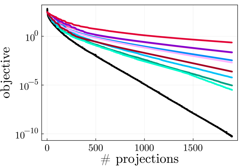
(a) $n=100$, $l=0.1$, $u=10$, $M=50$

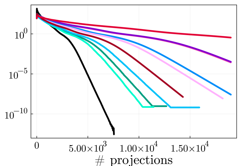
(b) $n=50$, $l=0.1$, $u=1000$, $M=100$

Figure 1: Maximum likelihood estimate, problem (45)

Low-rank matrix completion

We consider a famous low-rank matrix completion problem in the form

$$\min_{X\in\mathbbm{R}^{n\times n}}\frac{1}{2}\|P_{\Omega}(X-A)\|^{2}_{F}\quad\text{subject to}\quad\|X\|_{*}\leqslant r,$$ (46)

where $\Omega$ is a subset of indices $(i,j)$ and $r$ is the supposed maximum rank. To project onto the spectral ball $\mathcal{C}=\{X\colon\|X\|_{*}\leqslant r\}$, computing the singular value decomposition (SVD) is required, making it the most computationally expensive operation in this setting.

We created matrix $A$ by multiplying matrices $U$ and $V^{\top}$, where $U$ and $V$ are $n$-by-$r$ matrices with entries sampled from a normal distribution. The subset $\Omega$ was randomly chosen as a fraction of $\frac{1}{5}n^{2}$ entries from $[n]\times[n]$. The obtained results are depicted in Figure 2, where we solely compared the number of computed SVDs.

AdProxGD  (1.2, 0.5)  (1.5, 0.8)  (1.1, 0.5)  (1.2, 0.9)
(1.1, 0.9)  (1.5, 0.5)  (1.2, 0.8)  (1.1, 0.8)  (1.5, 0.9)

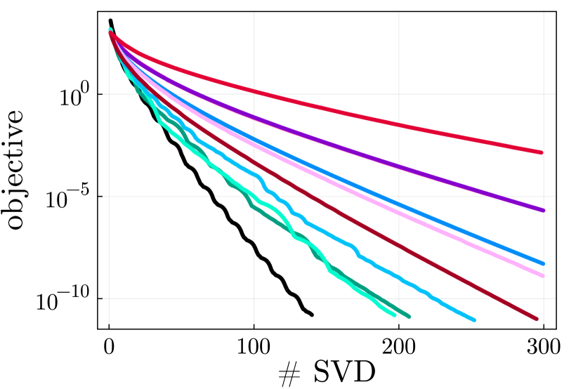
(a) $n=100$, $r=20$

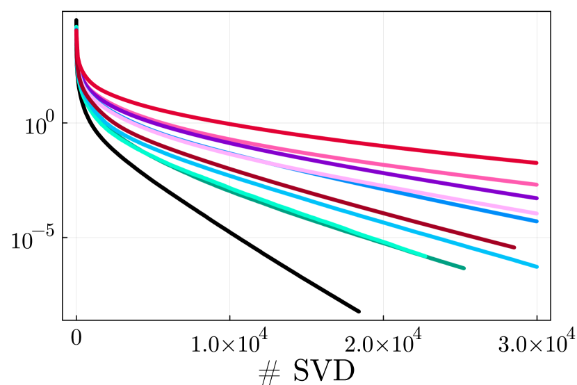
(b) $n=200$, $r=20$

Figure 2: Low-rank matrix completion, problem (46)

Minimal length piecewise-linear curve subject to linear constraints.

We consider [BV04, Example 10.4], where we want to minimize the length of a piecewise-linear curve passing through $n$ points in $\mathbb{R}^{2}$ with coordinates $(1,x_{1}),\dots,(n,x_{n})$ while satisfying linear constraints $Ax=b$, where $x=(x_{1},\dotsc,x_{n})$. Given $A\in\mathbbm{R}^{m\times n}$ and $b\in\mathbbm{R}^{m}$, this can be modeled as

$$\min_{x\in\mathbbm{R}^{n}}(1+x_{1})^{\nicefrac{{1}}{{2}}}+\sum_{i=1}^{n-1}(1+(x_{i+1}-x_{i})^{2})^{\nicefrac{{1}}{{2}}}\quad\text{subject to}\quad Ax=b.$$ (47)

While applying the proximal gradient method, the most computationally expensive operation is computing the projection onto $\mathcal{C}=\{x\colon Ax=b\}$. Assuming that $A$ is full rank with $m\leqslant n$, this projection can be computed as $P_{\mathcal{C}}z=z-A^{\top}(AA^{\top})^{-1}(Az-b)$.

In comparison, we focused solely on the number of computed projections. We generated a random $m$-by-$n$ matrix $A$ and random vector $w$ with entries sampled from a normal distribution and set $b=Aw$.

AdProxGD  (1.2, 0.5)  (1.5, 0.8)  (1.1, 0.5)  (1.2, 0.9)
(1.1, 0.9)  (1.5, 0.5)  (1.2, 0.8)  (1.1, 0.8)  (1.5, 0.9)

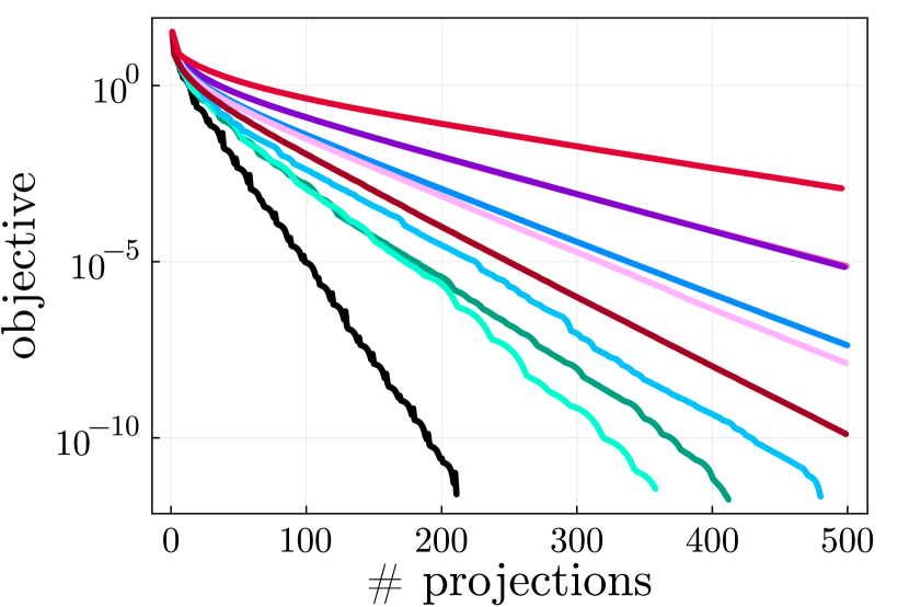
(a) $m=50$, $n=200$

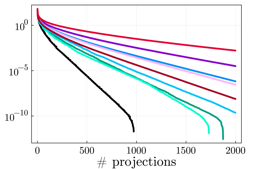
(b) $m=50$, $n=500$

Figure 3: Minimal length piecewise-linear curve, problem (47)

Nonnegative matrix factorization.

We want to solve the matrix factorization problem subject to nonnegative constraints:

$$\min_{U,V\in\mathbbm{R}^{n\times r}_{+}}f(U,V)=\frac{1}{2}\|UV^{\top}-A\|^{2}_{F},$$ (48)

where $A$ is a given $n$-by-$n$ low-rank matrix. Although nonconvex, this problem is famously well-tackled by first-order methods. In each iteration, the gradient $\nabla f(x)$ involves 3 matrix-matrix multiplications, whereas evaluating the objective $f(x)$ only requires 1. Note that for the last iteration of the linesearch, the computed matrix product can be reused to compute the gradient for the next iteration.

We created matrix $A$ by multiplying matrices $B$ and $C^{\top}$, where $B$ and $C$ are $n$-by-$r$ matrices with entries sampled from a normal distribution. Negative entries in both matrices $B$ and $C$ were then set to zero. The results are presented in Figure 4, where the number of gradients roughly means the number of 3 matrix-matrix multiplications.

AdProxGD  (1.2, 0.5)  (1.5, 0.8)  (1.1, 0.5)  (1.2, 0.9)
(1.1, 0.9)  (1.5, 0.5)  (1.2, 0.8)  (1.1, 0.8)  (1.5, 0.9)

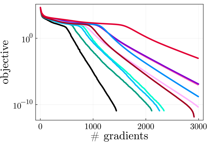
(a) $n=100$, $r=20$

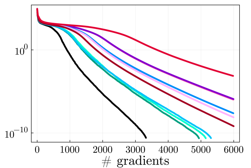
(b) $n=100$, $r=30$

Figure 4: Nonnegative matrix factorization, problem (48)

Dual of the entropy maximization problem.

Consider the entropy maximization problem subject to linear constraints

$$\min\sum_{i=1}^{n}x_{i}\log x_{i}\quad\text{subject to $Ax\leqslant b$,\quad$\sum_{i=1}^{n}x_{i}=1$, and $x_{i}>0$, }$$ (49)

where $A\in\mathbbm{R}^{m\times n}$. Its dual problem is given by

$$\min_{\lambda\in\mathbbm{R}^{m}_{+},\mu\in\mathbbm{R}}e^{-\mu-1}\sum_{i=1}^{n}e^{-a_{i}^{\top}\lambda}+\langle b,\lambda\rangle+\mu,$$ (50)

where $a_{i}\in\mathbbm{R}^{m}$ is the $i$-th column of $A$ (the derivation is provided in [BV04, Chapter 5.1.6]).

AdProxGD  (1.2, 0.5)  (1.5, 0.8)  (1.1, 0.5)  (1.2, 0.9)
(1.1, 0.9)  (1.5, 0.5)  (1.2, 0.8)  (1.1, 0.8)  (1.5, 0.9)

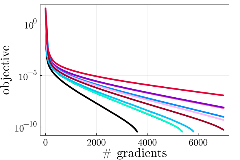
(a) $m=500$, $n=100$

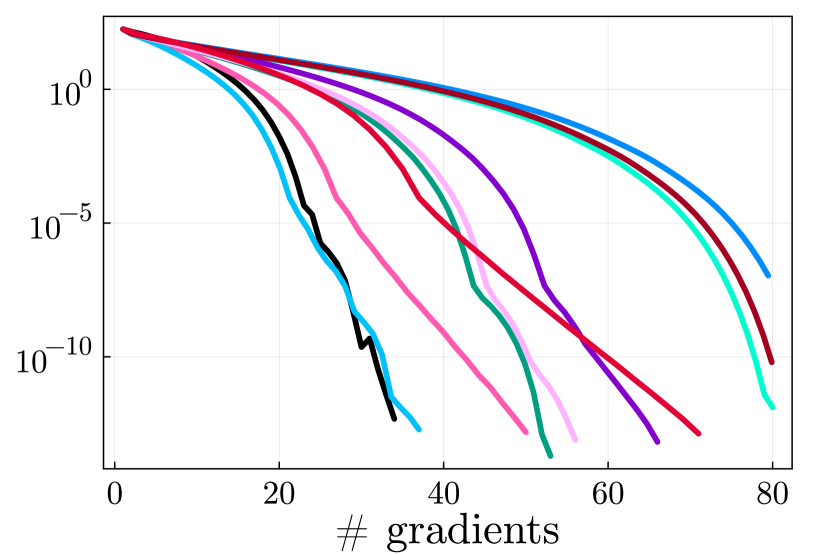
(b) $m=100$, $n=500$

Figure 5: Dual of the entropy maximization, problem (50)

It is the latter problem (50) that we solved. We generated $m$-by-$n$ matrix $A$ with entries sampled from a normal distribution. Then we generated a random $w\in\mathbbm{R}^{n}$ from the unit simplex and set $b=Aw$. Each gradient requires two matrix-vector multiplication, while the objective only one (and, as before, the last one can be reused for the next gradient). The results are presented in Figure 5, where the number of gradients roughly means the number of 2 matrix-vector multiplications.

Conclusion.

Based on our preliminary experiments, it is evident that AdProxGD indeed performs better. To our surprise, a few specific pairs $(r,s)$ consistently outperform the rest among ProxGD with linesearch. We are not aware of any theoretical finding that would confirm this evidence.

Appendix

Lemma 16.

The function $f$ defined in (8) satisfies the following properties:

1. $f$ is convex.

2. $f^{\prime}$ is $L$-Lipschitz with $L=1$.

3. $f$ is locally strongly convex, i.e., for any bounded set $\mathcal{X}$ there exists a constant $\mu_{\mathcal{X}}>0$ such that $|f^{\prime}(x)-f^{\prime}(y)|\geqslant\mu_{\mathcal{X}}|x-y|$ for any $x,y\in\mathcal{X}$.

4. $|f^{\prime}(x)|\leqslant G$ with $G=2$.

5. $f$ is $2$-Lipschitz.

Proof.

First, let us find $f^{\prime}$ and $f^{\prime\prime}$:

$$f^{\prime}(x)=\begin{cases}x,&x\in[-1,1]\\ \frac{ax}{1+|x|},&x\not\in[-1,1]\end{cases},\qquad f^{\prime\prime}(x)=\begin{cases}1,&x\in(-1,1)\\ \frac{a}{(1+|x|)^{2}},&x\not\in[-1,1]\end{cases},$$

so indeed $a=2$ and $b=2\log 2-\frac{3}{2}$. Convexity of $f$ follows from the fact that $f^{\prime\prime}(x)>0$ for any $x$. Lipschitzness of $f^{\prime}$ follows directly from the bound $f^{\prime\prime}(x)\leqslant 1$ for all $x$. Similarly, local strong convexity follows from the bound $f^{\prime\prime}(x)\geq\frac{1}{\max_{z\in\mathcal{X}}(1+|z|)^{2}}\eqqcolon\mu_{\mathcal{X}}$ for any $x\in\mathcal{X}$. Finally, the last two properties trivially follow from the expression for $f^{\prime}(x)$. ∎

Proof of Theorem 1.

Let us choose $x^{0}=r+2$ with a sufficiently large $r>6c$. This readily implies that

$$x^{1}=x^{0}-\frac{2x^{0}}{1+x^{0}}=\frac{x^{0}(x^{0}-1)}{x^{0}+1}>x^{0}-2=r.$$

Our goal is to show that the iterates follow a very specific pattern. Namely, we prove that for all $k\geqslant 0$,

$$\operatorname{sign}(x^{2k})=\operatorname{sign}(x^{2k+1}),\quad\operatorname{sign}(x^{2k+2})\neq\operatorname{sign}(x^{2k}),\quad|x^{2k+2}|>2|x^{2k+1}|>|x^{2k}|.$$

If this condition holds true, then the sequence $(x^{k})$ must be divergent.

First, observe that if $|x^{k}|,|x^{k-1}|\geqslant r$ and $\operatorname{sign}(x^{k})=\operatorname{sign}(x^{k-1})$, then the smoothness estimate admits a simple expression:

$$L_{k} =\frac{|f^{\prime}(x^{k})-f^{\prime}(x^{k-1})|}{|x^{k}-x^{k-1}|}=\frac{2\left|\frac{x^{k}}{1+|x^{k}|}-\frac{x^{k-1}}{1+|x^{k-1}|}\right|}{|x^{k}-x^{k-1}|}=\frac{2\left|\frac{|x^{k}|}{1+|x^{k}|}-\frac{|x^{k-1}|}{1+|x^{k-1}|}\right|}{||x^{k}|-|x^{k-1}||}$$

$$=\frac{2}{(1+|x^{k}|)(1+|x^{k-1}|)}<\frac{2}{r(1+|x^{k}|)}.$$

Therefore, in that case $\alpha_{k}|f^{\prime}(x^{k})|>\frac{r(1+|x^{k}|)}{2c}|f^{\prime}(x^{k})|=\frac{r|x^{k}|}{c}>3|x^{k}|$. Since $\operatorname{sign}(f^{\prime}(x^{k}))=\operatorname{sign}(x^{k})$, it implies that $|x^{k+1}|>2|x^{k}|$ and $\operatorname{sign}(x^{k+1})\neq\operatorname{sign}(x^{k})$.

Next, if $|x^{k}|,|x^{k-1}|\geqslant r>3$ with $|x^{k}|\geqslant 2|x^{k-1}|$ and $\operatorname{sign}(x^{k})\neq\operatorname{sign}(x^{k-1})$, then we have $\frac{2|x^{k}|}{1+|x^{k}|}>\frac{3}{2}$ and

$$L_{k} =\frac{|f^{\prime}(x^{k})-f^{\prime}(x^{k-1})|}{|x^{k}-x^{k-1}|}=\frac{2\left|\frac{x^{k}}{1+|x^{k}|}-\frac{x^{k-1}}{1+|x^{k-1}|}\right|}{|x^{k}-x^{k-1}|}=\frac{2\left(\frac{|x^{k}|}{1+|x^{k}|}+\frac{|x^{k-1}|}{1+|x^{k-1}|}\right)}{|x^{k}|+|x^{k-1}|}$$

$$>\frac{3}{|x^{k}|+|x^{k-1}|}>\frac{3}{|x^{k}|+\frac{1}{2}|x^{k}|}\geqslant\frac{2}{|x^{k}|}.$$

This implies $\alpha_{k}<\frac{|x^{k}|}{2c}\leqslant\frac{|x^{k}|}{2}$. Since $\operatorname{sign}(f^{\prime}(x^{k}))=\operatorname{sign}(x^{k})$ and $\frac{\alpha_{k}}{1+|x^{k}|}\leqslant\frac{|x^{k}|}{2(1+|x^{k}|)}<\frac{1}{2}$, we conclude that $\operatorname{sign}(x^{k+1})=\operatorname{sign}(x^{k})$ and

$$|x^{k+1}|=\left|x^{k}-\alpha_{k}\frac{x^{k}}{1+|x^{k}|}\right|=|x^{k}|\left(1-\frac{\alpha_{k}}{1+|x^{k}|}\right)>\frac{1}{2}|x^{k}|.$$

As $x^{0}$ and $x^{1}$ satisfy the first case, by induction we deduce that all iterates $(x^{k})$ follow the described pattern. ∎

Acknowledgments.

The authors would like to thank Puya Latafat, who found a subtle error in the convergence proof of $(x^{k})$ in Theorem 3 in the first version of this manuscript.

References

- [Arm66] Larry Armijo “Minimization of functions having Lipschitz continuous first partial derivatives” In Pacific J. Math. 16.1 Mathematical Sciences Publishers, 1966, pp. 1–3 DOI: 10.2140/pjm.1966.16.1
- [BB88] Jonathan Barzilai and Jonathan M. Borwein “Two-point step size gradient methods” In IMA J Numer Anal 8.1 Oxford University Press (OUP), 1988, pp. 141–148 DOI: 10.1093/imanum/8.1.141
- [BN16] José Yunier Bello Cruz and Tran T.A. Nghia “On the convergence of the forward–backward splitting method with linesearches” In Optim. Methods Softw. 31.6 Taylor & Francis, 2016, pp. 1209–1238
- [BV04] Stephen Boyd and Lieven Vandenberghe “Convex Optimization” Cambridge University Press, 2004 DOI: 10.1017/cbo9780511804441
- [CP10] Antonin Chambolle and Thomas Pock “A first-order primal-dual algorithm for convex problems with applications to imaging” In J Math Imaging Vis 40.1 Springer ScienceBusiness Media LLC, 2010, pp. 120–145 DOI: 10.1007/s10851-010-0251-1
- [DM23] Aaron Defazio and Konstantin Mishchenko “Learning-rate-free learning by D-adaptation” In Proceedings of the 40th International Conference on Machine Learning 202, 2023, pp. 7449–7479 URL: https://proceedings.mlr.press/v202/defazio23a.html
- [DHS11] John Duchi, Elad Hazan and Yoram Singer “Adaptive subgradient methods for online learning and stochastic optimization” In J. Mach. Learn. Res. 12, 2011, pp. 2121–2159
- [Gol62] A.. Goldstein “Cauchy’s method of minimization” In Numer. Math. 4.1 Springer ScienceBusiness Media LLC, 1962, pp. 146–150 DOI: 10.1007/bf01386306
- [Gri23] Benjamin Grimmer “Provably faster gradient descent via long steps”, 2023 arXiv:2307.06324
- [IHC23] Maor Ivgi, Oliver Hinder and Yair Carmon “DoG is SGD’s best friend: A parameter-free dynamic step size schedule” In Proceedings of the 40th International Conference on Machine Learning 202, 2023, pp. 14465–14499
- [KMJ23] Ahmed Khaled, Konstantin Mishchenko and Chi Jin “DoWG unleashed: An efficient universal parameter-free gradient descent method”, 2023 arXiv:2305.16284
- [Lat+23] Puya Latafat, Andreas Themelis, Lorenzo Stella and Panagiotis Patrinos “Adaptive proximal algorithms for convex optimization under local Lipschitz continuity of the gradient”, 2023 arXiv:2301.04431
- [Mal19] Yura Malitsky “Golden ratio algorithms for variational inequalities” In Math. Program. 184.1-2 Springer ScienceBusiness Media LLC, 2019, pp. 383–410 DOI: 10.1007/s10107-019-01416-w
- [MM20] Yura Malitsky and Konstantin Mishchenko “Adaptive gradient descent without descent” In Proceedings of the 37th International Conference on Machine Learning 119, Proceedings of Machine Learning Research PMLR, 2020, pp. 6702–6712 arXiv: http://proceedings.mlr.press/v119/malitsky20a.html
- [MS10] H. McMahan and Matthew Streeter “Adaptive bound optimization for online convex optimization” In Proceedings of the 23rd Annual Conference on Learning Theory (COLT), 2010
- [Sal17] Saverio Salzo “The variable metric forward-backward splitting algorithm under mild differentiability assumptions” In SIAM J. Optim. 27.4 Society for Industrial & Applied Mathematics (SIAM), 2017, pp. 2153–2181 DOI: 10.1137/16m1073741
- [TV22] Marc Teboulle and Yakov Vaisbourd “An elementary approach to tight worst case complexity analysis of gradient based methods” In Math. Program. 201.1-2 Springer ScienceBusiness Media LLC, 2022, pp. 63–96 DOI: 10.1007/s10107-022-01899-0
- [VMC21] Maria-Luiza Vladarean, Yura Malitsky and Volkan Cevher “A first-order primal-dual method with adaptivity to local smoothness” In NeurIPS 34, 2021, pp. 6171–6182 arXiv:2110.15148