Unifying heat transport model for the transition between buoyancy-dominated and Lorentz-force-dominated regimes in quasistatic magnetoconvection

Abstract

In magnetoconvection, the flow of electromagnetically conductive fluid is driven by a combination of buoyancy forces, which create the fluid motion due to thermal expansion and contraction, and Lorentz forces, which distort the convective flow structure in the presence of a magnetic field. The differences in the global flow structures in the buoyancy-dominated and Lorentz-force-dominated regimes lead to different heat transport properties in these regimes, reflected in distinct dimensionless scaling relations of the global heat flux (Nusselt number Nu) versus the strength of buoyancy (Rayleigh number Ra) and electromagnetic forces (Hartmann number Ha). Here, we propose a theoretical model for the transition between these two regimes for the case of a quasistatic vertical magnetic field applied to a convective fluid layer confined between two isothermal, a lower warmer and an upper colder, horizontal surfaces. The model suggests that the scaling exponents $\gamma$ in the buoyancy-dominated regime, $\mbox{\rm{Nu}}\sim\mbox{\rm{Ra}}^{\gamma}$, and $\xi$ in the Lorentz-force-dominated regime, $\mbox{\rm{Nu}}\sim(\mbox{\rm{Ha}}^{-2}\mbox{\rm{Ra}})^{\xi}$, are related as $\xi=\gamma/(1-2\gamma)$, and the onset of the transition scales with $\mbox{\rm{Ha}}^{-1/\gamma}\mbox{\rm{Ra}}$. These theoretical results are supported by our Direct Numerical Simulations for $10\leq\mbox{\rm{Ha}}\leq 2000$, Prandtl number $\mbox{\rm{Pr}}=0.025$ and Ra up to $10^{9}$ and data from the literature.

1 Introduction

Magnetoconvection (MC) governs most astro- and geophysical systems and is relevant to various engineering applications [25, 7]. The former include, for instance, outer layers of stars and liquid metal planetary cores [12], examples of the latter comprise liquid-metal batteries, induction heating, casting, liquid-metal cooling for nuclear fusion reactors and semiconductor crystal growth [6]. MC occurs in an electrically conducting fluid that is subjected both to a magnetic field and an imposed temperature gradient. The buoyancy forces induce convective fluid motion due to thermal expansion and contraction, while the magnetic field affects this motion and distorts the global flow structure through the Lorentz force, which eventually influences the heat transport in the system. The resulting main two control parameters, the strength of the imposed thermal driving and that of the external magnetic field, are encoded in independent dimensionless groups, the Rayleigh number Ra and Hartmann number Ha, respectively.

One of the key objectives in MC research is to provide scaling relations for the heat transport through the system, represented in dimensionless form by the Nusselt number Nu, as a function of Ra and Ha. However, the heat transport scaling relations also depend on the flow configuration, including the angle between the magnetic field and gravity, the geometry of the container and the boundary conditions (BCs), and on whether the buoyancy forces dominate over the Lorentz forces in the system or vice versa. This inherent complexity results in the need, at least in principle, to derive separate heat transport scaling relations to describe each specific flow regime itself and transitions between distinct regimes. The considerable difficulty of doing so in a coherent manner is exacerbated by non-universal scaling relations even within specific regimes – the scaling relations in the buoyancy-dominated and Lorentz-force-dominated regimes themselves change with the control parameters, and transitions between the different regimes are also non-universal.

The objective of this paper is to offer a unifying heat transport model for the transition between the buoyancy-dominated and Lorentz-force-dominated regimes in quasistatic MC. We focus on Rayleigh–Bénard convection (RBC) [2] with an applied vertical magnetic field and assume that the magnetic field is constant in the entire domain, without being affected by a fluid motion or finite magnetic diffusion. The model uses the theoretical predictions by Grossmann and Lohse [9, 10, 24] for RBC without magnetic field and transfers the approach by Ecke and Shishkina [8, §3.3] for transitions in rotating RBC to the case of RBC with a vertical magnetic field. To verify the proposed model, we compare the theoretical predictions with results for liquid metal MC obtained by direct numerical simulation (DNS) carried out by us and others [16, 27, 3, 26], as well as experiments [5, 13, 28, 26]. In addition, we carried out simulations for a different working fluid at higher Prandtl number Pr to compare our DNS data with that from Ref. [15]. The predictions of the proposed model agree well the experimental and DNS data.

2 Model for the transition between the buoyancy dominated and Lorentz force dominated regimes

We consider a layer of electrically conducting fluid confined between two infinitely wide and long plates, driven by a buoyancy force generated by an imposed vertical temperature difference between the top and bottom plates, and subjected to a uniform vertically orientated magnetic field. When the magnetic field is weak compared to the buoyancy force, we recover classical RBC scaling for the dimensionless convective heat flux $\mbox{\rm{Nu}}-1$, that is, the total dimensionless heat flux Nu less its conductive contribution, $\mbox{\rm{Nu}}-1\sim(\mbox{\rm{Ra}}/\mbox{\rm{Ra}}_{c,b})^{\gamma}\sim\mbox{\rm{Ra}}^{\gamma}$, for an exponent $\gamma$, where where $\mbox{\rm{Ra}}_{c,b}$ is the critical Ra for RBC bulk onset for a given container geometry. When the Lorentz force is strong compared to the buoyancy force, we expect a similar scaling law $\mbox{\rm{Nu}}-1\sim\left(\mbox{\rm{Ra}}/\mbox{\rm{Ra}}_{c,L}\right)^{\xi}$, for an exponent $\xi$. Here, the dependence on the critical Rayleigh number $\mbox{\rm{Ra}}_{c,L}$ in the Lorentz-force-dominated regime is kept due to its dependence on Ha, that can be obtained from the linear stability theory [4] $\mbox{\rm{Ra}}_{c,L}\sim\mbox{\rm{Ha}}^{2}$, with no dependence on the Prandtl number.

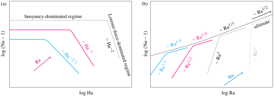
Figure 1: Scalings of $\mbox{\rm{Nu}}-1$ versus (a) Ha and (b) Ra, according to the theory.

Although these buoyancy-dominated and Lorentz-force-dominated scaling laws appear disconnected, they are intrinsically linked under the assumption that they must overlap at some intermediate region between the two extreme regimes, where neither the influence of the Lorentz force or buoyancy force on the convective heat transport can be ignored. At the transition between these regimes, the two corresponding scaling laws will scale in the same way,

$$\mbox{\rm{Ra}}^{\gamma}\sim\mbox{\rm{Nu}}-1\sim(\mbox{\rm{Ha}}^{-2}\mbox{\rm{Ra}})^{\xi},$$ (1)

To construct a relationship between the two scaling exponents $\gamma$ and $\xi$, we assume that this cross-over occurs when the thicknesses of the thermal and viscous boundary layers (BLs) scale in the same way, motivated by the observation that the viscous layer is nested within the thermal BL in the Lorentz-force-dominated regime and vice versa in the buoyancy-dominated regime. In a domain of height $H$ over a semi-infinite plate, the average thermal BL thickness from laminar Prandtl-Blasius boundary layer theory [18, 21] is $\delta_{\theta}=H/(2\mbox{\rm{Nu}})\sim\mbox{\rm{Nu}}^{-1}$, while the laminar viscous BL influenced by a vertical magnetic field is the Hartmann layer [11, 7], $\delta_{\small\mbox{\rm{Ha}}}=cH/\mbox{\rm{Ha}}\sim\mbox{\rm{Ha}}^{-1}$, where $c$ is a constant. Assuming that $\delta_{\theta}\sim\delta_{\small\mbox{\rm{Ha}}}$ at the transition implies $\mbox{\rm{Nu}}\sim\mbox{\rm{Ha}}$. Since this transition is seen to typically occur at high Nusselt numbers, meaning $\mbox{\rm{Nu}}\approx\mbox{\rm{Nu}}-1$, we obtain

$$\mbox{\rm{Ha}}\sim\mbox{\rm{Nu}}\sim\mbox{\rm{Ra}}^{\gamma}\sim\mbox{\rm{Ra}}^{\xi}\mbox{\rm{Ha}}^{-2\xi}\sim\mbox{\rm{Ra}}^{-2\xi\gamma+\xi},$$ (2)

resulting in the following relationship between the exponents,

$$\xi={\gamma/(1-2\gamma)},\quad\textrm{or}\quad\gamma={\xi/(1+2\xi)}.$$ (3)

One can see that a larger (smaller) exponent in one regime requires a larger (smaller) exponent the other regime, and that $\gamma$ is always smaller than $1/2$.

In Fig. 1 we present a sketch of the proposed scaling relations for $(\mbox{\rm{Nu}}-1)$ versus Ha (Fig. 1 a) and Ra (Fig. 1 b), according to the relations (3). Once $\gamma$ is known for any specific Pr, the exponent $\xi$ can be calculated from Eq. (3). These scalings can then be used define coordinates $(\mbox{\rm{Nu}}-1)\mbox{\rm{Ra}}^{-\gamma}$ and $\mbox{\rm{Ha}}^{-1/\gamma}\mbox{\rm{Ra}}$ with respect to which the heat transport dependence for different values of Ha and Ra collapse onto a master curve, as sketched in Fig. 2. The transition then should take place in a Rayleigh-number range that scales as $\mbox{\rm{Ha}}^{1/\gamma}$.

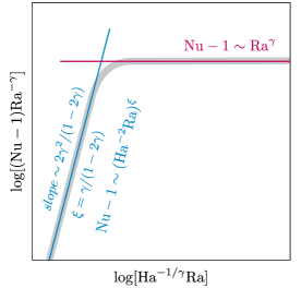
Figure 2: Schematic representation of the normalized convective heat transport $\mbox{\rm{Nu}}-1$ displaying the transition from the Lorentz-force-dominated regime, $\mbox{\rm{Nu}}-1\sim(\mbox{\rm{Ha}}^{-2}\mbox{\rm{Ra}})^{\xi}$, to the buoyancy-dominated regime, $\mbox{\rm{Nu}}-1\sim\mbox{\rm{Ra}}^{\gamma}$, according to our model. The scaling exponents $\xi$ and $\gamma$ follow Eq. (3), while the transition scales with $\mbox{\rm{Ha}}^{-1/\gamma}\mbox{\rm{Ra}}$.

To close the model, a theoretical prediction for either $\gamma$ or $\xi$ must be made. The former is readily available through Grossmann–Lohse (GL) theory [9, 10, 24] for RBC without magnetic field, applicable here in the buoyancy-dominated regime. For any given Pr and Ra-range, the theory provides accurate predictions of the value of $\gamma$, for containers of aspect ratio $\Gamma\gtrsim 1$. For $\Gamma\ll 1$, the data can be rescaled according to the method suggested in [22, 1], which we do not discuss here, as in the present study $\Gamma=1$.

3 Status Quo – experimental and numerical data.

To verify the theoretical model we compare its predictions against data obtained from experiments of liquid-metal MC [5, 13, 28, 26] and DNS conducted by us and others [16, 27, 3, 26]. However, before doing so we provide a brief overview of the data collated from the literature and produced by us to demonstrate the considerable challenges that arise when trying to draw firm conclusions on the scaling of the heat transport with Ha and Ra.

We simulate an incompressible, viscous buoyancy-driven flow of an electrically conducting fluid in the presence of an imposed magnetic field for very small magnetic Reynolds number $\mbox{\rm{Re}}_{m}\ll 1$ and magnetic Prandtl number $\mbox{\rm{Pr}}_{m}\ll 1$ by numerically solving the MC equations within the Oberbeck–Boussinessq and quasistatic approximation,

$$\frac{\partial\bm{u}}{\partial t}+\bm{u}\cdot{\nabla}\bm{u}+{\nabla}p = \sqrt{\frac{\mbox{\rm{Pr}}}{\mbox{\rm{Ra}}}}[{\nabla}^{2}\bm{u}+\mbox{\rm{Ha}}^{2}(\bm{j}\times\bm{e}_{B})]+T\bm{e}_{z},\quad\ \$$ (4)

$$\frac{\partial T}{\partial t}+\bm{u}\cdot{\nabla}T = \frac{1}{\sqrt{\mbox{\rm{Ra}}\mbox{\rm{Pr}}}}{\nabla}^{2}T,$$ (5)

$${\nabla}\cdot\bm{u} = 0,$$ (6)

$$\bm{j} = -{\nabla}\phi+\bm{u}\times\bm{e}_{B},$$ (7)

$${\nabla}^{2}\phi = {\nabla}\cdot(\bm{u}\times\bm{e}_{B}).$$ (8)

where $\bm{u}$ is the velocity, $T$ the temperature, $p$ the kinematic pressure, $\bm{j}$ the electric current density, $\phi$ the electric potential, and $\bm{e}_{z}$ and $\bm{e}_{B}$ are unit vectors that point, respectively, upward (opposite to gravity) and in the direction of the magnetic field $\bm{B}=B_{0}\bm{e}_{B}$. The magnetic field is aligned with the buoyancy force, $\bm{e}_{B}=\bm{e}_{z}$.

Equations  (4)–(8) have been non-dimensionalized using the container height $H$, the free-fall velocity $u_{f\!f}\equiv(\alpha gH\Delta)^{1/2}$, the free-fall time $t_{f\!f}\equiv H/u_{f\!f}$, the temperature difference between the bottom and top plates, $\Delta\equiv T_{+}-T_{-}$, and the external magnetic field strength, $B_{0}$, as units of length, velocity, time, temperature and magnetic field strength, respectively. The dimensionless control parameters are the Rayleigh number Ra, the Prandtl number Pr, and the Hartmann number Ha,

$$\mbox{\rm{Ra}}\equiv~{}\frac{\alpha g\Delta H^{3}}{\kappa\nu},\qquad\mbox{\rm{Pr}}\equiv~{}\frac{\nu}{\kappa},\qquad\mbox{\rm{Ha}}\equiv~{}B_{0}H\sqrt{\frac{\sigma}{\rho\nu}}\ ,$$ (9)

where $\sigma$ is the electrical conductivity, $\rho$ the mass density, $\alpha$ the thermal expansion coefficient, $g$ the acceleration due to gravity, $\nu$ the kinematic viscosity, and $\kappa$ the thermal diffusivity. We apply no-slip BCs for the velocity at all boundaries, $\bm{u}=0$, constant temperatures at the end-faces, i.e., $T=T_{+}$ at the bottom plate at $z=0$ and $T=T_{-}$ at the top plate at $z=H$, and adiabatic BC at the side walls, $\partial T/\partial\bm{n}=0$, where $\bm{n}$ is the vector orthogonal to the surface. All solid boundaries are considered electrically insulated; Neumann BCs for the electric potential are $\partial\phi/\partial\bm{n}=0$. The simulation domain is cubic of height $H$, width $W$, length $L$, $H=W=L$, i.e. has aspect ratio $\Gamma\equiv L/H=1$. Most simulations are carried out for liquid metals such as GaInSn at $\mbox{\rm{Pr}}=0.025$, for Ra up to $10^{9}$ and Ha up to $2000$. Some DNS are conducted also for $\mbox{\rm{Pr}}=8$, to extend the parameter range studied in Ref. [15]. In the bulk, spatial flow fluctuations are resolved down to 2-5, occasionally 10 Kolmogorov miscroscales, near the rigid walls we resolve the thermal and Hartmann BLs [23]. Our DNSs have been carried out with an MC extension of goldfish [14, 20, 19]. Further details of the simulations are provided in appendix A.

In Fig. 3 we present $\mbox{\rm{Nu}}-1$ as a function of Ra (Fig. 3 a-b) and Ha (Fig. 3 c-d), respectively, from our DNS, experimental [5, 13, 28, 26] and DNS data [16, 3, 26] for liquid metals, $0.025\leq\Pr\leq 0.029$ (Fig. 3 b, d) and a fluid with $\mbox{\rm{Pr}}=8$ (Fig. 3 a, c). In addition, in Fig. 3 (b, d), we plot for comparison the DNS data [27] for free-slip BCs. In Fig. 3 (a-b) one can see that Nu generally increases with growing Ra, but with different slopes for different Ha, which are steeper for larger Ha. In the double logarithmic plots of Fig. 3 (a-b), the curves of the $(\mbox{\rm{Nu}}-1)$-vs.-Ra dependences for different Ha approach each other when Ra increases. In Fig. 3 (c-d) one can see that Nu remains to be almost unaffected by the magnetic field for relatively small Ha, but for a strong Lorentz force (large Ha) they gradually decrease with growing Ha. Here, again, the decreasing slopes are different for different Ra, and the transition to the regime, where the heat transport is affected by the magnetic field, depends on Ra. In summary, the data in Fig. 3 look rather different in different experiments and DNS. In what follows, we show that our model results in a collapse of all data points on a single master curve.

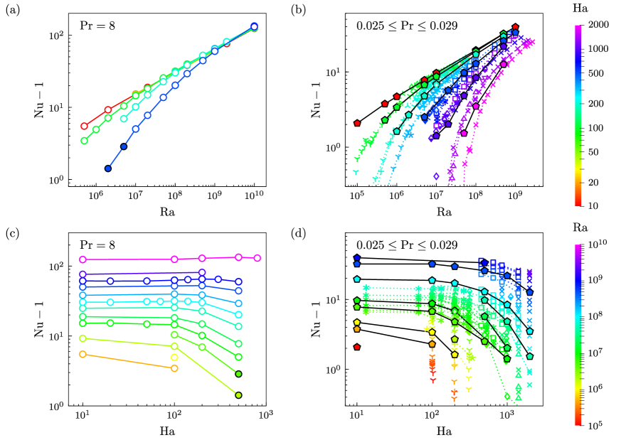
Figure 3: The dimensionless convective heat transport, i.e., $\mbox{\rm{Nu}}-1$, as functions of (a, b) Ra and (c-d) Ha, for (a, c) $\mbox{\rm{Pr}}=8$ and (b, d) $0.025\leq\Pr\leq 0.029$. The color scales are according to (a-b) Ha and (c-d) Ra.

4 Model validation

We now validate the model using the data presented in Fig. 3. To calculate the scaling exponent $\gamma$ in the buoyancy-dominated regime, for the considered Pr and Ra-ranges, we use GL theory, which gives $\gamma$ about 0.30 for $\mbox{\rm{Pr}}=8$ and about 0.31 for $\mbox{\rm{Pr}}=0.025$. These values agree very well with fits to data for the Ra-ranges in the buoyancy-dominated regime for both values of Pr, see appendix A for further details. Using Eq. (3) with $\gamma=0.30$ for $\mbox{\rm{Pr}}=8$ and $\gamma=0.31$ for $\mbox{\rm{Pr}}=0.025$, we calculate the exponent $\xi$ in the Lorentz-force-dominated regime, which equals $\xi=0.75$ for $\mbox{\rm{Pr}}=8$ and $\xi\approx 0.82$ for $\mbox{\rm{Pr}}=0.025$. In Fig. 4 we plot all data presented previously Fig. 3 using the coordinates suggested by our model and visualised in Fig. 2. This results in a clear collapse of the data onto master curves for $\mbox{\rm{Pr}}=8$ (Fig. 4 a) and $0.025\leq\mbox{\rm{Pr}}\leq 0.029$ (Fig. 4 b). Some deviation of the data from the master curve in Fig. 4 (b) is observed when Ra is relatively small and the flow is in the wall-mode regime, that is, before the onset of bulk convection where heat transport is confined to the near-wall region. Since the influence of no-slip side-walls is outside of the scope of our model, the observed deviations are expected in this regime.

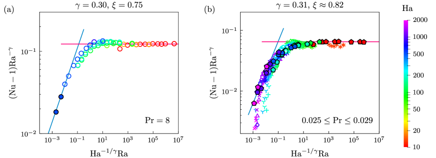
Figure 4: All data from Fig. 3 follow master scaling curves if plotted as Fig. 2 suggests, for (a) $\mbox{\rm{Pr}}=8$ and (b) $0.025\leq\mbox{\rm{Pr}}\leq 0.029$. The values of $\gamma$ are calculated from GL theory, and the values of $\xi$ are calculated from Eq. (3). Pink and blue lines show the predictions of the slopes in the buoyancy and Lorentz-force-dominated regimes, respectively. The symbols have the same meaning as in Fig. 3.

5 Conclusion

In conclusion, we have proposed a heat transport model for the transition between the buoyancy- and Lorentz-force-dominated regimes of vertical MC. We validated the model using our DNS and data available in the literature. We wish to emphasize that the proposed model is parameter-free. For a given Pr and Ra-range, one can calculate the scaling exponent in the buoyancy-dominated regime, using GL theory. Then, using Eq. (3), one can calculate the scaling exponent $\xi$ in the Lorentz-force-dominated regime and collapse the data on a master curve by rescaling the coordinate axes as in Fig. 2. The model can in principle be extended to include the effect of a fluctuating magnetic field, this merely results in an adjustment of the prefactors.

Appendix A Appendix

A.1 Numerical simulations

All direct numerical simulations have been carried using the direct numerical solver goldfish [14], which has been widely used in previous studies of different convective flows. The new version of the code that applies a fourth-order finite-volume discretisation on staggered grids and a third-order Runge–Kutta time marching scheme [20, 19] has been extended to simulate magnetoconvective flows, where a consistent and conservative scheme [17] is utilised to calculate the current density and the Lorentz force. The three-dimensional DNS are performed using staggered grids that provide fine resolution in the core part of the domain and near the rigid walls [23], to resolve the thermal and Hartmann boundary layers. The main parameters and key observables of the simulations are summarised in table 1.

The DNS dataset comprises 37 simulations to cover the necessary ranges in Ha and Ra. To obtain a dataset this large within the available resources, a compromise had to be made in terms of the bulk resolution. Hence a number of simulations do not resolve scales close to the Kolmogorov microscale. To ensure accurate predictions of mean Nu, grid refinement studies have been done for key simulations (marked by * in the $h_{\text{DNS}}/h_{\text{K}}$ column). For these cases, changing the grid resolution by a factor of at least 2.5 resulted in changes of Nu by less than 1% over a long-time average.

A.2 Grossmann-Lohse scaling

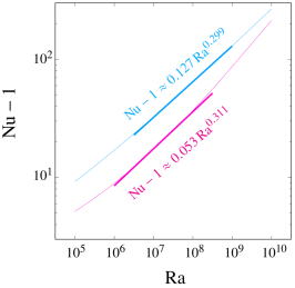
Figure 5: Predictions of GL theory [9, 10, 24] (thin lines) for $\mbox{\rm{Nu}}-1$ versus Ra scaling relations in RBC without magnetic field, for $\Pr=8$ (blue) and $\Pr=0.025$ (pink). The power fits for the considered Ra-ranges are highlighted with thick lines of the corresponding colors.

Figure 5 shows a comparison between the predictions of Grossmann-Lohse theory [9, 10, 24] for the dependence of the dimensionless heat transport $\mbox{\rm{Nu}}-1$ on the Rayleigh number Ra, $\mbox{\rm{Nu}}-1=A\,\mbox{\rm{Ra}}^{\gamma}$ for $\Pr$-dependent prefactor $A$. Fits to data have been carried out for $3\times 10^{6}\leqslant 10^{9}$ for $\Pr=0.025$ and $3\times 10^{6}\leqslant 10^{9}$ for $\Pr=8$. As can been seen from the data presented in fig. 5, the theoretical predictions agree very well with the data.

A.3 Flow and temperature field visualisations

Figures 6 and 7 present visualisations the velocity magnitude and temperature, respectively, at an instant in time during statistically steady evolution in the magnetically dominated and the buoyancy-dominated regimes. In both figures, the respective panels (a) correspond to $\mbox{\rm{Ra}}=10^{7}$, $\mbox{\rm{Ha}}=1000$, panels (b) to $\mbox{\rm{Ra}}=10^{9}$, $\mbox{\rm{Ha}}=10$. As can be seen from a comparison of the flow and temperature field between both regimes, both velocity and temperature fluctuate on much smaller scales in the buoyancy-dominated regime. The magnetically dominated regime is shows strong vertical flows near the walls, and we note the absence of plumes in the temperature field.

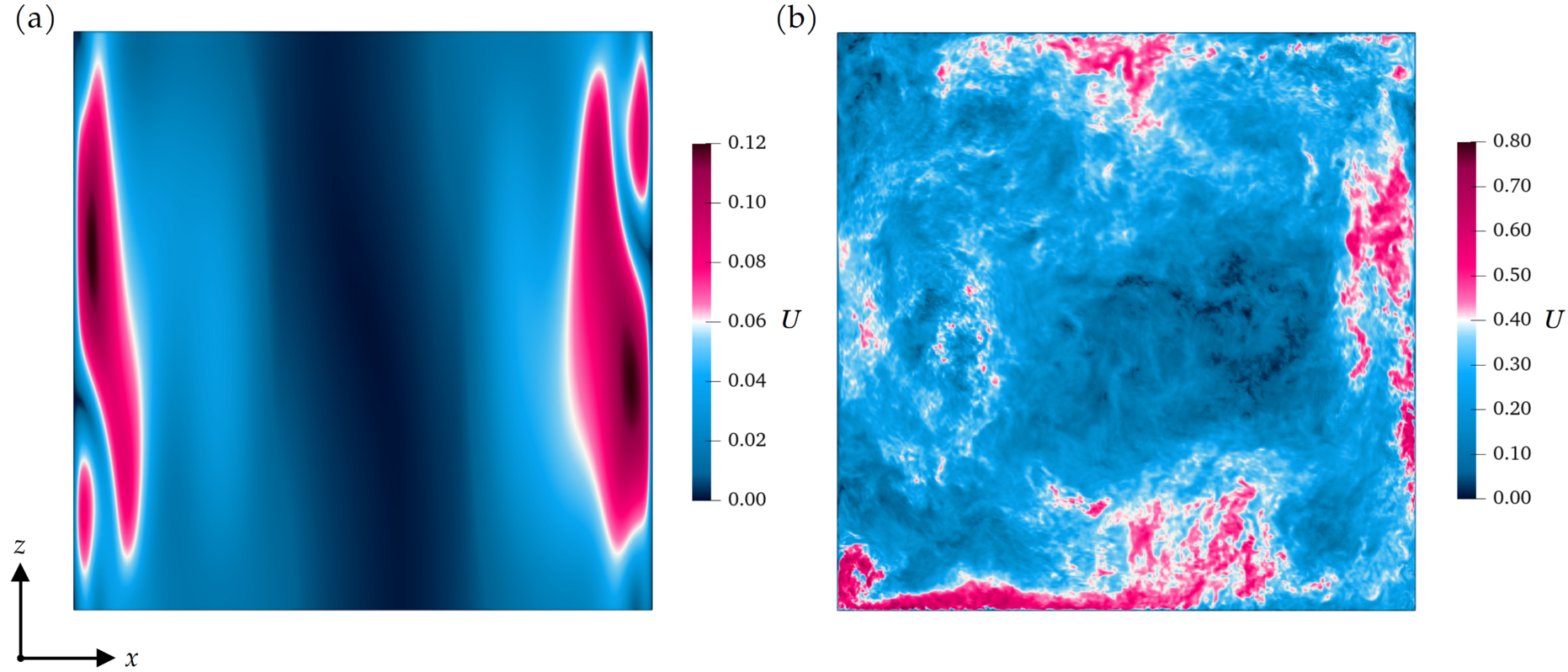
Figure 6: Instantaneous velocity magnitude $U$ shown on the $y$ mid-plane for (a) $Ra=10^{7}$, $Ha=1000$ and (b) $Ra=10^{9}$, $Ha=10$.

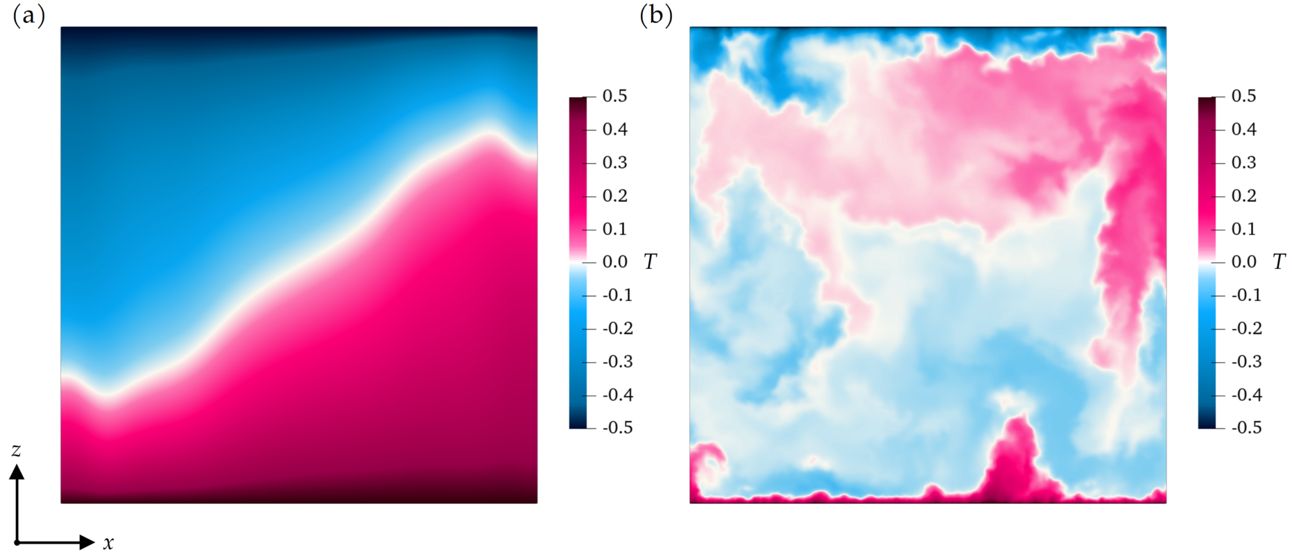
Figure 7: Instantaneous temperature field $T$ shown on the $y$ mid-plane for (a) $Ra=10^{7}$, $Ha=1000$ and (b) $Ra=10^{9}$, $Ha=10$.

$\Pr$	Ha	Ra	Nu	$\sigma_{\mbox{\rm{Nu}}}$	$N_{x}$	$N_{y}$	$N_{z}$	$T_{run}$	$\mathcal{N}_{\theta}$	$\mathcal{N}_{\text{Ha}}$	$h_{\text{DNS}}/h_{\text{K}}$
$8$	500	$2.0\times 10^{6}$	2.42	0.01	100	100	300	350	90	8	0.40
	500	$5.0\times 10^{6}$	3.86	0.02	100	100	300	550	70	8	0.60
0.025	10	1.0$\times 10^{5}$	3.08	0.04	150	150	200	40	49	36	1.06
	10	5.0$\times 10^{5}$	4.76	0.21	150	150	200	45	37	36	1.76
	10	1.0$\times 10^{6}$	5.70	0.32	150	150	200	65	33	36	2.20
	10	5.0$\times 10^{6}$	8.77	0.67	150	150	200	100	25	36	3.64
	10	1.0$\times 10^{7}$	10.68	0.78	150	150	200	160	22	36	4.49*
	10	1.0$\times 10^{8}$	20.42	1.98	250	250	350	50	29	67	5.42
	10	5.0$\times 10^{8}$	33.18	1.47	250	250	350	90	21	67	8.76
	10	1.0$\times 10^{9}$	40.47	2.32	350	350	450	40	25	87	8.64*
	100	5.0$\times 10^{5}$	3.29	0.06	200	200	250	20	60	10	1.07
	100	1.0$\times 10^{6}$	4.39	0.14	200	200	250	30	50	10	1.34
	100	5.0$\times 10^{6}$	7.74	0.56	200	200	250	40	35	10	2.40
	100	1.0$\times 10^{7}$	9.69	0.44	200	200	250	60	31	10	3.09*
	100	1.0$\times 10^{8}$	19.72	1.36	220	220	300	45	24	13	5.81
	100	5.0$\times 10^{8}$	33.10	1.76	250	250	350	65	21	16	8.45*
	200	1.0$\times 10^{6}$	2.62	0.03	220	220	350	120	101	15	1.13
	200	2.0$\times 10^{6}$	3.69	0.01	220	220	350	225	84	15	1.46
	200	5.0$\times 10^{6}$	5.78	0.22	220	220	350	225	66	15	2.06
	200	1.0$\times 10^{7}$	7.87	0.39	220	220	350	160	56	15	2.65*
	200	1.0$\times 10^{8}$	18.06	1.82	250	250	400	100	42	17	5.07
	200	5.0$\times 10^{8}$	30.56	2.63	250	250	400	100	32	17	8.66*
	500	5.0$\times 10^{6}$	3.51	0.06	220	220	350	650	86	9	1.82
	500	2.0$\times 10^{7}$	6.70	0.34	220	220	350	190	61	9	3.02
	500	5.0$\times 10^{7}$	10.73	0.64	220	220	350	300	48	9	4.27*
	500	1.0$\times 10^{8}$	13.88	0.76	250	250	400	500	48	11	4.74
	500	5.0$\times 10^{8}$	26.75	1.77	250	250	400	150	34	11	8.36
	500	1.0$\times 10^{9}$	34.44	2.59	250	250	400	250	30	11	10.64*
	1000	1.0$\times 10^{7}$	2.41	0.26	220	220	300	600	90	5	1.92*
	1000	2.0$\times 10^{7}$	3.02	0.08	220	220	300	1300	80	5	2.30
	1000	5.0$\times 10^{7}$	5.84	0.37	220	220	300	500	56	5	3.02
	1000	1.0$\times 10^{8}$	9.39	0.51	220	220	300	1100	44	5	3.77
	1000	5.0$\times 10^{8}$	22.78	1.35	220	220	300	60	18	5	6.44*
	2000	5.0$\times 10^{7}$	2.53	0.09	250	250	400	90	116	5	2.20
	2000	1.0$\times 10^{8}$	4.50	0.11	250	250	400	160	86	5	2.68
	2000	5.0$\times 10^{8}$	13.60	0.63	250	250	400	220	49	5	4.47*

Table 1: Details on the conducted DNS, including the standard deviation $\sigma_{\small\mbox{\rm{Nu}}}$ of the Nusselt number Nu, the number of nodes $N_{x}$, $N_{y}$, $N_{z}$ in the directions $x$, $y$ and $z$, respectively; the number of simulation free-fall times used for averaging $T_{run}$; the number of the nodes within the thermal boundary layer, and within the Hartmann boundary layer $\mathcal{N}_{\text{Ha}}$; the Kolmogorov microscale, $h_{\text{K}}$, and the relative mean grid stepping, $h_{\text{DNS}}/h_{\text{K}}$. Simulations marked by * are those for which grid refinement studies have been completed.

References

- [1] G. Ahlers, E. Bodenschatz, R. Hartmann, X. He, D. Lohse, P. Reiter, R.J.A.M. Stevens, R. Verzicco, M. Wedi, S. Weiss, X. Zhang, L. Zwirner, and O. Shishkina. Aspect ratio dependence of heat transfer in a cylindrical Rayleigh–Bénard cell. Phys. Rev. Lett., 128:084501, 2022.
- [2] G. Ahlers, S. Grossmann, and D. Lohse. Heat transfer and large scale dynamics in turbulent Rayleigh–Bénard convection. Rev. Mod. Phys., 81:503–537, 2009.
- [3] R. Akhmedagaev, O. Zikanov, D. Krasnov, and J. Schumacher. Turbulent Rayleigh–Bénard convection in a strong vertical magnetic field. J. Fluid Mech., 895:R4, 2020.
- [4] S. Chandrasekhar. Hydrodynamic and Hydromagnetic Stability. Clarendon Press, 1961.
- [5] S. Cioni, S. Chaumat, and J. Sommeria. Effect of a vertical magnetic field on turbulent Rayleigh–Bénard convection. Phys. Rev. E, 62:R4520–R4523, 2000.
- [6] P. A. Davidson. Magnetohydrodynamics in materials processing. Annu. Rev. Fluid Mech., 31:273–300, 1999.
- [7] P. A. Davidson. Introduction to Magnetohydrodynamics. Cambridge University Press, 2016.
- [8] R. E. Ecke and O. Shishkina. Turbulent rotating Rayleigh–Bénard convection. Annu. Rev. Fluid Mech., 55:603–638, 2023.
- [9] S. Grossmann and D. Lohse. Scaling in thermal convection: A unifying theory. J. Fluid Mech., 407:27–56, 2000.
- [10] S. Grossmann and D. Lohse. Thermal convection for large Prandtl numbers. Phys. Rev. Lett., 86:3316–3319, 2001.
- [11] J. Hartmann and F. Lazarus. Hg-dynamics ii. experimental investigations on the flow of mercury in a homogeneous magnetic field. Det Kgl Danske Videnskabernes Selskkab Math-fys Medd, 15(7):1–45, 1937.
- [12] C. A. Jones. Planetary magnetic fields and fluid dynamos. Annu. Rev. Fluid Mech., 43:583–614, 2011.
- [13] E. M. King and J. M. Aurnou. Magnetostrophic balance as the optimal state for turbulent magnetoconvection. Proc. Natl. Acad. Sci., 112:990–994, 2015.
- [14] G. L. Kooij, M. A. Botchev, E. M.A. Frederix, B. J. Geurts, S. Horn, D. Lohse, E. P. van der Poel, O. Shishkina, R. J. A. M. Stevens, and R. Verzicco. Comparison of computational codes for direct numerical simulations of turbulent Rayleigh–Bénard convection. Comp. Fluids, 166:1–8, 2018.
- [15] Z. L. Lim, K. L. Chong, G.-Y. Ding, and K.-Q. Xia. Quasistatic magnetoconvection: heat transport enhancement and boundary layer crossing. J. Fluid Mech., 870:519–542, 2019.
- [16] W. Liu, D. Krasnov, and J. Schumacher. Wall modes in magnetoconvection at high Hartmann numbers. J. Fluid Mech., 849:R2, 2018.
- [17] M.-J. Ni and J.-F. Li. A consistent and conservative scheme for incompressible MHD flows at a low magnetic Reynolds number. Part III: On a staggered mesh. J. Comput. Phys., 231:281–298, 2012.
- [18] L. Prandtl. Über Flüssigkeitsbewegung bei sehr kleiner Reibung. In Verhandlungen des III. Int. Math. Kongr., Heidelberg, 1904, pages 484–491. Teubner, 1905.
- [19] P. Reiter, O. Shishkina, D. Lohse, and D. Krug. Crossover of the relative heat transport contributions of plume ejecting and impacting zones in turbulent Rayleigh–Bńard convection. Europhys. Lett., 134:34002, 2021.
- [20] P. Reiter, X. Zhang, and O. Shishkina. Flow states and heat transport in Rayleigh–Bénard convection with different sidewall boundary conditions. J. Fluid Mech., 936:A32, 2022.
- [21] H. Schlichting. Boundary layer theory. McGraw-Hill, 1979.
- [22] O. Shishkina. Rayleigh–Bénard convection: The container shape matters. Phys. Rev. Fluids, 6:090502, 2021.
- [23] O. Shishkina, R. J. A. M. Stevens, S. Grossmann, and D. Lohse. Boundary layer structure in turbulent thermal convection and its consequences for the required numerical resolution. New J. Phys., 12:075022, 2010.
- [24] R. J. A. M. Stevens, E. P. van der Poel, S. Grossmann, and D. Lohse. The unifying theory of scaling in thermal convection: The updated prefactors. J. Fluid Mech., 730:295–308, 2013.
- [25] N. O. Weiss and M. R. E. Proctor. Magnetoconvection. Cambridge University Press, 2014.
- [26] Y. Xu, S. Horn, and J. M. Aurnou. The transition from wall modes to multimodality in liquid gallium magnetoconvection. https://arxiv.org/pdf/2303.08966.pdf, 2023.
- [27] M. Yan, M. A. Calkins, S. Maffei, K. Julien, S. Tobias, and P. Marti. Heat transfer and flow regimes in quasi-static magnetoconvection with a vertical magnetic field. J. Fluid Mech., 877:1186–1206, 2019.
- [28] T. Zürner, F. Schindler, T. Vogt, S. Eckert, and J. Schumacher. Flow regimes of rayleigh–bénard convection in a vertical magnetic field. J. Fluid Mech., 894:A21, 2020.