Fusion regression methods with repeated functional data

Abstract

Linear regression and classification methods with repeated functional data are considered. For each statistical unit in the sample, a real-valued parameter is observed over time under different conditions. Two regression methods based on fusion penalties are presented. The first one is a generalization of the variable fusion methodology based on the 1-nearest neighbor. The second one, called group fusion lasso, assumes some grouping structure of conditions and allows for homogeneity among the regression coefficient functions within groups. A finite sample numerical simulation and an application on EEG data are presented.
Keywords. linear models, regression, classification, variable fusion, fused lasso, multivariate functional data, repeated functional data, group lasso

1 Introduction

Let $X$ be a functional random variable valued in some Hilbert space of real-valued functions defined on the time interval $[0,T]$, $T>0$. Without loss of generality, we assume that this space is the set of squared integrable functions $L_{2}([0,T])$ (Ramsey and Silverman, , 2005). The setting we consider in this paper assumes that $X$ is observed under $p$ different conditions $\{\mathscr{C}_{1},\ldots,\mathscr{C}_{p}\}$, $p\geq 1$. For instance, these conditions can represent times or/and locations (regions) in some metrical space $(\mathscr{S},d)$, typically $(\mathbb{R}^{s},\|\cdot\|_{2})$, for some natural integer $s\geq 1$. Thus, proximity or grouping structures of conditions can be considered through the distance $\color[rgb]{0,0,0}d(\cdot,\cdot)$. As an example, EEG data (Ruiz et al., , 2021) measure the brain activity through the electric field intensity over a time interval of $T=500ms$ and at different regions of the brain using $p=28$ electrodes/sensors evenly distributed (Figure 1).

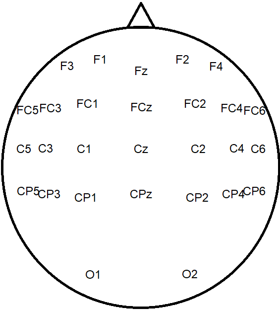
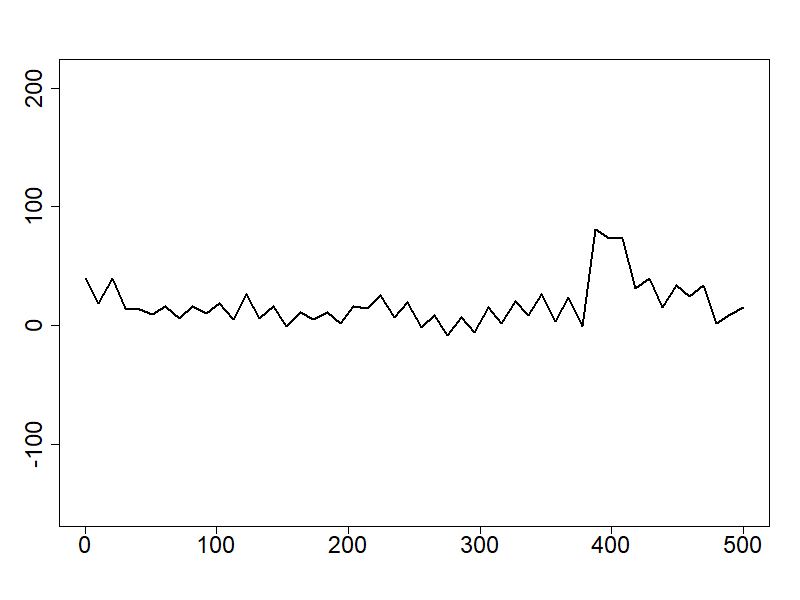
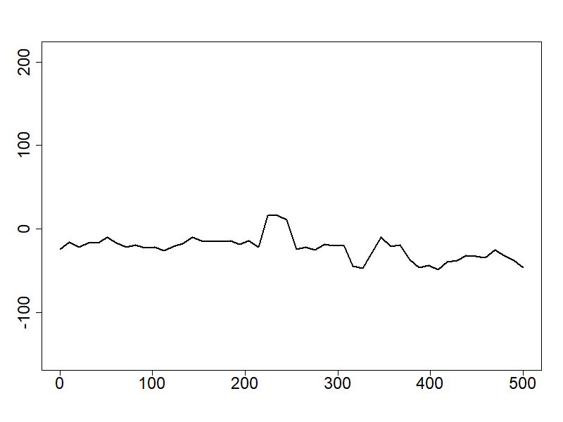
F1: F2: F3: F4: $\vdots$ $\vdots$ O1: O2:

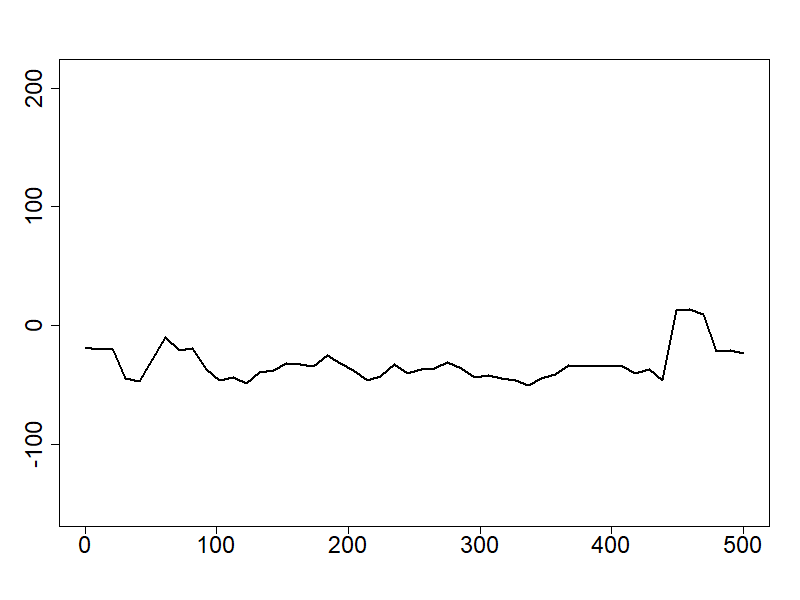
Figure 1: FingerMovements data. Each subject is represented by $p=28$ EEG recordings (right) corresponding to $28$ sensors located on the scalp (left).

Let denote with $X^{(j)}$ the observation of $X$ under the condition $\mathscr{C}_{j}$, $j=1,\ldots,p$, and with $\mathbf{X}$, the random vector

$$\mathbf{X}=(X^{(1)},\ldots,X^{(p)})^{\top}.$$

The realizations of $X^{(1)},\ldots,X^{(p)}$ are known as repeated functional data. Principal components analysis (PCA) were developed to deal with the dependency between the components $X^{(j)}$. In Chen and Müller, (2012) the authors use a double PCA exploiting the metric structure of the space of conditions $\{\mathscr{C}_{1},\ldots,\mathscr{C}_{p}\}$ belong. In Jacques and Preda, (2014) that structure is ignored and $\mathbf{X}$ is viewed as a $p$-dimensional functional random vector of which principal components are used for clustering and visualization.

In this paper we are interested in the estimation of the linear regression model with scalar or binary response $Y$ and predictor $\mathbf{X}$ taking into account the topology of the measurement conditions through some neighborhood or group belonging relationship (defined eventually by the distance $d$). Thus, as a difference of the classical framework of linear regression with multivariate functional data, in our approach, we use the structure of the space the conditions of measurement of components $X^{(j)}$ belong, for the model estimation. To the best of our knowledge, there are no proposed methods in the multivariate functional data framework that explicitly take into account the information carried by the spatial feature of data. The existing contributions mainly consider $\mathbf{X}$ as a $p$-dimensional functional vector and methodologies were designed to take into account the dependence between the dimensions of $\mathbf{X}$ (see e.g Yi et al., (2022), Górecki et al., (2015), Beyaztas and Lin Shang, (2022), Moindjié et al., (2022)).

We tackle the problem from the interpretation point of view in the sense that components $X^{(j)}$’s spatially close should provide similar information in the regression model. Our motivation application is on electroencephalography recordings (EEG) classification. Each subject is writing a text and the electric field intensity $X$ is measured simultaneously at $p=28$ spatial positions (sensors) of the scalp during $T=500ms$. Two groups of subjects are considered: the right-handed $(Y=0)$ and left-handed $(Y=1)$ writers. The question is to know and interpret in what measure the ability of a person to be left or right-handed is associated with some different activity of the brain. In statistical terms, to understand the relationship between $Y$ and $\mathbf{X}$.

The standard functional linear regression model assumes that there exists $\beta^{(0)}\in\mathbb{R}$ and the regression coefficient function $\beta=(\beta^{(1)},\ldots,\beta^{(p)})^{\top}\in\mathscr{H}=\{L_{2}([0,T])\}^{p}$ such that

$$\mathbb{E}(Y|\mathbf{X})\approx{\color[rgb]{0,0,0}\color[rgb]{0,0,0}\beta^{(0)}+\sum_{j=1}^{p}\langle X^{(j)},\beta^{(j)}\rangle_{L_{2}}}$$ (1)

where

$$\langle X^{(j)},\beta^{(j)}\rangle_{L_{2}}=\int_{0}^{T}X^{(j)}(t)\beta^{(j)}(t)dt,$$

for $j=1,\ldots,p$.
If $\{(X_{i},Y_{i})\}_{i=1:n}$ is an i.i.d. sample of size $n$, $n\geq 1$, drawn from the same distribution as $(\mathbf{X},Y)$ and $\{(x_{i},y_{i})\}_{i=1:n}$ is an observation of that sample, the estimation of the model (1) is based on the minimization of the mean of the squared errors (MSE), that is,

$$(\hat{\beta}^{(0)},\hat{\beta})=\operatorname*{arg\,min}_{(\psi^{(0)},\psi)\in\mathbb{R}\times\mathscr{H}}\frac{1}{n}\sum_{i=1}^{n}\left(y_{i}-\left(\psi^{(0)}+\sum_{j=1}^{p}\langle x_{i}^{(j)},\psi^{(j)}\rangle_{L_{2}}\right)\right)^{2}.$$ (2)

Because of the non-invertibility of the covariance operator, the direct estimation of the coefficient $\beta$ under the minimization of the MSE criterion is an ill-posed problem (Cardot et al., , 1999). The principal component regression (PCR) and the partial least squares (PLS) have been successful alternatives in this case (see e.g Escabias et al., (2005), Aguilera et al., (2006), Preda and Saporta, (2002), Moindjié et al., (2022)). However, in these approaches, the estimated coefficient functions are sometimes difficult to interpret: why do two components $X^{(j)}$ and $X^{(j^{\prime})}$ that are associated to close conditions $\mathscr{C}_{j}$ and $\mathscr{C}_{j^{\prime}}$, i.e. the distance $d(\mathscr{C}_{j},\mathscr{C}_{j^{\prime}})$ is small, have very different associated coefficient functions $\beta^{(j)}$ and $\beta^{(j^{\prime})}$? This situation occurs especially when $p$ is large. In Godwin, (2013), the authors propose to add the constraint $\mathscr{P}=\sum_{j=1}^{p}||\psi^{(j)}||_{{}_{L_{2}}}$ in the regression model. In this case, $\mathscr{P}$ is a generalization to functional multivariate variables of the penalty group lasso (GL), originally introduced in the multivariate data case (Meier et al., (2008), Yuan and Lin, (2006)).

This penalty leads to achieving a trade-off between a minimum number of contributing components $X^{(j)}$ and model fit. Our hypothesis is that closeness between components $X^{(j)}$, in the sense of the distance $d$ between the corresponding conditions $\mathscr{C}_{j}$, can help for a better interpretation of $\beta$. For this purpose, the fusion penalty was introduced in the finite multivariate setting in Land and Friedman, (1997).

Let $v$ be a surjective function, $v:\{\mathscr{C}_{1},\ldots,\mathscr{C}_{p}\}\mapsto\{1,\ldots,K\}$, $K\leq p$, and define the fusion penalty (in the functional framework) as

$$\mathscr{P}(\beta)=\sum_{k=1}^{K}\sqrt{\sum_{j\in\mathscr{I}_{k}}\left|\left|\beta^{(j)}-\bar{\beta}_{\mathscr{I}_{k}}\right|\right|^{2}_{L_{2}}},$$

where for each $k=1:K$, $\mathscr{I}_{k}=\left\{j:v(\mathscr{C}_{j})=k\right\}$ and $\bar{\beta}_{\mathscr{I}_{k}}(t)=\frac{1}{|\mathscr{I}_{k}|}\sum_{j\in\mathscr{I}_{k}}\beta^{(j)}(t)$ for $t\in[0,T]$ and $|\mathscr{I}_{k}|$ denotes the cardinal of $\mathscr{I}_{k}$ for $k=1,\ldots,p$. Then, the proximity between conditions $\mathscr{C}_{1},\ldots,\mathscr{C}_{p}$ can be integrated through the function $v$ and the distance $d$ : $v^{-1}(k)$ represents all the conditions closest to $\mathscr{C}_{k}$. Obviously, this penalty favors close dimensions of ${\bf X}$ to have similar corresponding dimensions of the regression function (the $\beta^{(j)}$’s functions).

To our knowledge, this penalty has not been explored in the case of regression with repeated functional variables (nor multivariate functional variables). In the classical multivariate setting, the models that have this penalty are known as the variable fusion model (FU) (Land and Friedman, , 1997) and, when a lasso penalty is added, as the fused lasso method (FL) (Tibshirani et al., , 2005). More recently, the group fusion method (GFL) introduced in Bleakley and Vert, (2011) extended this penalty from unique conditions to groups of conditions. However, in these cases, the function $v$ has been oriented as a way to integrate consecutive conditions (or dimensions), i.e. $v$ is defined as $v(\mathscr{C}_{j})=j+1$, for $1\leq j\leq p-1$ and $v(\mathscr{C}_{p})=p$. Even if this case can be well-suited for the setting $\mathscr{S}\subset\mathbb{R}$ ($s=1$), it limits the number of applications as for multivariate locations, i.e. $s\geq 2$. In this case, the function $v$ can be defined through the distance $d$ and can be used naturally to extend the variable fusion method (Land and Friedman, , 1997) to such a spatial structure of components of ${\bf X}$.

In this paper, we introduce two new fusion-like penalties for the functional linear regression estimation under the mean squares error criterion. The first one is an extension of the variable fusion method (FU) where the 1-nearest neighbor graph (1-NN) is used to define $v$. We show that the estimation of FU in this setting is equivalent to a group lasso method such as those studied in Godwin, (2013). The second method we introduce takes into account a more general grouping structure of conditions. We call it the group fusion lasso (GFUL) model. It allows also us to test the equality among the dimensions of the coefficient regression function belonging to the same cluster of conditions.

The paper is organized as follows. Section 2 presents the proposed methodologies and their estimation strategies using basis function expansion techniques. A comparison study of the two methods and the group lasso approach is performed using simulated data in Section 3.1. A real data application from the EEG classification task is presented in Section 3.2. The paper ends with a discussion in Section 4.

2 Two new fusion methods for linear regression with multivariate functional data

Without loss of generality assume that $\mathbf{X}$ and $Y$ are zero mean random variables. Moreover, we consider that $\{(x_{i},y_{i})\}_{i=1,\ldots,n}$ is an observation of $\{(X_{i},Y_{i})\}_{i=1,\ldots,n}$, an i.i.d sample of size $n\geq 1$ drawn from the joint distribution as $(\mathbf{X},Y)$.
Under the zero mean assumption of $\bf X$ and $Y$, the intercept $\beta^{(0)}$ in (1) vanishes and the mean square criterion (2) becomes:

$$\hat{\beta}=\operatorname*{arg\,min}_{\psi\in\mathscr{H}}\frac{1}{n}\sum_{i=1}^{n}\left(y_{i}-\sum_{j=1}^{p}\langle x_{i}^{(j)},\psi^{(j)}\rangle_{L_{2}}\right)^{2}.$$

Remind that for each $i=1,\ldots,n$, $y_{i}\in\mathbb{R}$ and $x_{i}$ is a multivariate function defined on $[0,T]$,

$$x_{i}(t)=\left(x_{i}^{(1)}(t),\ldots,x_{i}^{(j)}(t),\ldots,x_{i}^{(p)}(t)\right)^{\top},\ \ \ t\in[0,T],$$

where each dimension $x_{i}^{(j)}$ is observed under the condition $\mathscr{C}_{j}$, $j=1,\ldots,p$.

Let us now introduce our first model of penalty based on distance among conditions.

2.1 Fusion method based on the neighbor relationship among conditions

The basic idea is that if two conditions $\mathscr{C}_{j}$ and $\mathscr{C}_{j^{\prime}}$ are close in the space $\mathscr{S}$ (with respect to distance $d$), then the contributions brought by the components $X^{(j)}$ and $X^{(j^{\prime})}$ in the linear model (1), i.e., $\beta^{(j)}$ and $\beta^{(j^{\prime})}$, might be comparable. Allowing for identical coefficients $\beta^{(j)}$ associated with close conditions, the variable fusion methodology is a candidate to obtain a parsimonious model and to compete with existing linear model approaches (Land and Friedman, (1997), Tibshirani et al., (2005), Bleakley and Vert, (2011)).
When the conditions $\mathscr{C}_{j}$ belong to $\mathbb{R}^{s}$ with $s\geq 2$, the distance $d$ defines a neighbor relationship between conditions and thus it can be used to estimate the regression coefficient functions accordingly. More precisely, following the ideas in Land and Friedman, (1997), the 1-nearest neighbor (1-NN) variable fusion model can be formulated as the following optimization problem:

$$\begin{split}\hat{\beta}_{\lambda}&=\operatorname*{arg\,min}_{\beta\in\mathscr{H}}\frac{1}{2}\sum_{i=1}^{n}\left(y_{i}-\sum_{j=1}^{p}\langle x_{i}^{(j)},\beta^{(j)}\rangle_{L_{2}}\right)^{2}+\lambda\sum_{j=1}^{p}||\beta^{(j)}-\beta^{(v(\mathscr{C}_{j}))}||_{L_{2}}\end{split}$$ (3)

where $\lambda\geq 0$, $v:\{\mathscr{C}_{1},\ldots,\mathscr{C}_{p}\}\to\{1,\ldots,p\}$ denotes the neighbor function

$$v(\mathscr{C}_{j})=\operatorname*{arg\,min}_{i\in\{1,\ldots,p\}\backslash\{j\}}d(\mathscr{C}_{i},\mathscr{C}_{j}),\;j=1,\ldots,p.$$ (4)

The function $v$ helps to integrate into the estimation process of $\beta$ the information brought by the conditions (locations, spatial distributions). Notice that if the set of $\operatorname*{arg\,min}$ in (4) is not unique, then we choose randomly or experimentally an element of this set.
For ease of notation, let denote with $\langle\cdot,\cdot\rangle_{\mathscr{H}}$ the inner product in $\mathscr{H}$ defined by :

$$\langle f,g\rangle_{\mathscr{H}}=\sum_{i=1}^{p}\langle f^{(i)},g^{(i)}\rangle_{L_{2}},$$

for all $f,g\in\mathscr{H}$.

The penalty function in (3) can then be rewritten as

$$\sum_{j=1}^{p}||\beta^{(j)}-\beta^{(v(\mathscr{C}_{j}))}||_{L_{2}}=||\mathbf{L}\beta||_{L_{2},1},$$

where $\mathbf{L}=\mathbf{W}-\mathbb{I}_{p\times p}$ and $\mathbf{W}=(w_{i,j})_{1\leq i\leq p,1\leq j\leq p}$ is the adjacency matrix with elements

$$w_{i,j}=\left\{\begin{array}[]{ll}1&\mbox{if $v(\mathscr{C}_{i})=j$ }\\ 0&\mbox{otherwise. }\end{array}\right.$$

$\mathbb{I}_{p\times p}$ is the $p\times p$ identity matrix and $||\cdot||_{L_{2},1}$ is the norm on $\mathscr{H}$ defined as :

$$||f||_{L_{2},1}=\sum_{i=1}^{p}||f^{(i)}||_{L_{2}},\;f\in\mathscr{H}.$$

For illustrative purposes, consider the toy example shown in Figure 2, with $\mathscr{S}\subset\mathbb{R}^{2}$ and $p=8$. It represents $p=8$ points corresponding to the conditions $\mathscr{C}_{j}\in\mathbb{R}^{2}$, $j=1,\ldots,p$. The neighborhood relationship among the conditions is given by the following $v$ function: $v(\mathscr{C}_{1})=8$, $v(\mathscr{C}_{2})=5$, $v(\mathscr{C}_{3})=4$, $v(\mathscr{C}_{4})=5,v(\mathscr{C}_{5})=4,v(\mathscr{C}_{6})=1,v(\mathscr{C}_{7})=1$ and $v(\mathscr{C}_{8})=1$.

Remark that the rank of the matrix $\mathbf{L}$ is generally lower than $p$, since symmetric relationships are possible (contrary to consecutive conditions case, see e.g Land and Friedman, (1997)). For example, Figure 2 shows that $\mathscr{C}_{1}$ is the neighbor of $\mathscr{C}_{8}$ and $\mathscr{C}_{8}$ is the neighbor of $\mathscr{C}_{1}$, the same for the couple $(\mathscr{C}_{5},\mathscr{C}_{4})$.

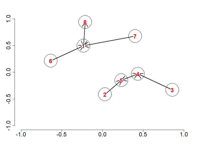
Figure 2: One nearest neighbor graph: $a\rightarrow b$ means $b$ is the neighbor of $a$.

Lemma 1.

If $r$ is the rank of the matrix $\mathbf{L}$, there exists a $r\times p$ full rank matrix $\mathbf{L}_{0}$ such as

$$||\mathbf{L}f||_{L_{2},1}=||\mathbf{L}_{0}f||_{L_{2},1},\;f\in\mathscr{H}.$$ (5)

Thus, $\mathbf{L}_{0}$ avoids redundancy. Its construction consists of finding the couples of rows corresponding to symmetric relations and then, for each such a couple, replace it with a row representing the double of the replaced ones. The rank of the matrix $\mathbf{L}$ coincides with the number of vertices of the undirected version of the 1-NN graph.
As an illustration, in our toy example (Figure 2), we have the following matrices

$$\mathbf{L}=\begin{pmatrix}-1&0&0&0&0&0&0&1\\ 0&-1&0&0&1&0&0&0\\ 0&0&-1&1&0&0&0&0\\ 0&0&0&-1&1&0&0&0\\ 0&0&0&1&-1&0&0&0\\ 1&0&0&0&0&-1&0&0\\ 1&0&0&0&0&0&-1&0\\ 1&0&0&0&0&0&0&-1\end{pmatrix}$$

and

$$\mathbf{L}_{0}=\begin{pmatrix}-2&0&0&0&0&0&0&2\\ 0&-1&0&0&1&0&0&0\\ 0&0&-1&1&0&0&0&0\\ 0&0&0&-2&2&0&0&0\\ 1&0&0&0&0&-1&0&0\\ 1&0&0&0&0&0&-1&0\end{pmatrix}.$$

Hence, lemma 1 implies that there’s an alternative reformulation of (3). Similarly to the variable fusion methodology (Land and Friedman, , 1997), Proposition 1 shows that (3) can be resolved using a lasso method.

Proposition 1.

The solution of (3) is given by

$$\hat{\beta}_{\lambda}=\mathbf{D}^{-1}\hat{\psi}_{\lambda},$$

where

$$\hat{\psi}_{\lambda}=\operatorname*{arg\,min}_{f\in\mathscr{H}}\frac{1}{2}\sum_{i=1}^{n}\left(y_{i}-\langle(\mathbf{D}^{-1})^{\operatorname*{\top}}x_{i},f\rangle_{\mathscr{H}}\right)^{2}+\lambda\sum_{j=1}^{r}||f^{(j)}||_{L_{2}},$$ (6)

$\mathbf{D}=\begin{pmatrix}\mathbf{L}_{0}\\ \mathbf{T}\end{pmatrix}$, $\mathbf{L}_{0}$ is the $r\times p$ reduced matrix of $\mathbf{L}$ and $\mathbf{T}$ is a $(p-r)\times p$ matrix which rows form a basis of the null space of $\mathbf{L}_{0}$, $\mathbf{L}_{0}\mathbf{T}^{\operatorname*{\top}}=\mathbf{0}_{r\times(p-r)}$ and $\mathbf{0}_{r\times(p-r)}$ is the $r\times(p-r)$ matrix of zeros.

Note that the estimation of the non-penalized part of $f$ in (6), $f^{(r+1)},\ldots,f^{(p)}$, might lead (putting maximum weights on the non-constrained part of $\beta$) to model overfitting. To fix this issue, we propose to modify the penalty term in (6) as:

$$||\mathbf{L}\beta||_{L_{2},1}+\frac{\sqrt{p-r}}{\eta}||\mathbf{T}\beta||_{L_{2},2},$$

where $\eta$ is the Frobenius matrix norm of $\mathbf{T}$, and $||\cdot||_{L_{2},2}$ denotes the Frobenius norm of $\mathscr{H}$:

$$||f||_{L_{2},2}=\sqrt{\sum_{i=1}^{p}||f^{(i)}||^{2}_{L_{2}}},$$

for $f\in\mathscr{H}$.
Thus, the optimization problem (6) becomes :

$$\hat{\psi}_{\lambda}=\operatorname*{arg\,min}_{f\in\mathscr{H}}\frac{1}{2}\sum_{i=1}^{n}\left(y_{i}-\langle(\mathbf{D}^{-1})^{\operatorname*{\top}}x_{i},f\rangle_{\mathscr{H}}\right)^{2}+\lambda\left(\sum_{j=1}^{r}||f^{(j)}||_{L_{2}}+\frac{\sqrt{p-r}}{\eta}\left(\sum_{j=r+1}^{p}||f^{(j)}||^{2}_{L_{2}}\right)^{1/2}\right).$$ (7)

This methodology is based on only one neighbor. In the next section, we introduce a similar methodology based on more than one neighbor, we called it the group fusion lasso.

2.2 The group fusion lasso

Let consider the example represented in Figure 3. In this example, we assume that the conditions are labeled according to $K=3$ groups: the yellow group $(\mathscr{C}_{3},\mathscr{C}_{4},\mathscr{C}_{7})$, the red group $(\mathscr{C}_{1},\mathscr{C}_{6},\mathscr{C}_{8})$ and the black group$(\mathscr{C}_{2},\mathscr{C}_{5})$. For this configuration, more than one neighbor must be considered. Indeed, the following sets $(\mathscr{C}_{1},\mathscr{C}_{6},\mathscr{C}_{8})$ $(\mathscr{C}_{3},\mathscr{C}_{4},\mathscr{C}_{7})$, $(\mathscr{C}_{2},\mathscr{C}_{5})$ have symmetric neighborhood relations (i.e. $\mathscr{C}_{8}$ has $(\mathscr{C}_{1},\mathscr{C}_{6})$ as neighbours, $\mathscr{C}_{6}$ has $(\mathscr{C}_{1},\mathscr{C}_{8})$ as neighbours, etc.). Rather than examining the interactions of the conditions individually, we propose in this section to test the resulting group relations.

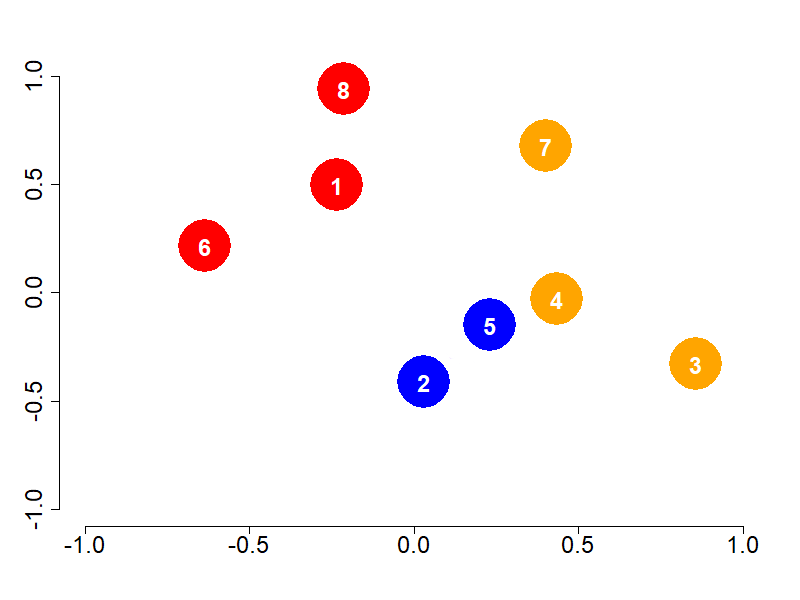
Figure 3: Conditions with grouping structure

The grouping structure of conditions is now given by the surjective function $v$,

$$v:\{\mathscr{C}_{1},\ldots,\mathscr{C}_{p}\}\to\{1,\ldots,K\},$$ (8)

where $K$ is a number of groups, $K\leq p$.
We recall the definition of the sets of index

$$\mathscr{I}_{k}=\{j\in\{1,\ldots,p\},\;v(\mathscr{C}_{j})=k\},\;k=1,\ldots,K.$$

Let denote the size of each group by

$$p_{k}=|\mathscr{I}_{k}|,\ \ \forall k\in 1,\ldots,K.$$

The idea behind the group fusion methodology (GFU) is to introduce criteria that favor having similar coefficients for the components corresponding to conditions belonging to the same group. In the example presented in Figure 3, $p=8$, $K=3$ and

• $v(\mathscr{C}_{1})=v(\mathscr{C}_{6})=v(\mathscr{C}_{8})=1$, the ”red” group,

• $v(\mathscr{C}_{2})=v(\mathscr{C}_{5})=2$, the ”black” group

• $v(\mathscr{C}_{3})=v(\mathscr{C}_{4})=v(\mathscr{C}_{7})=3$ the ”yellow” group.

Then, as in the lasso regularization framework, this estimation methodology forces the clusters of conditions to have close coefficient functions and, eventually, some of them be exactly the same:

$$\{\beta^{(1)}=\beta^{(6)}=\beta^{(8)}\}\ \ \mbox{and/or}\ \{\beta^{(2)}=\beta^{(5)}\}\ \mbox{and/or}\ \{\beta^{(3)}=\beta^{(4)}=\beta^{(7)}\}.$$

For this purpose, let modify the criterion (3) by adding a term penalty for each group $k$ of coefficient functions, $\mathscr{P}_{k}(\cdot)$, $k=1,\ldots,K$, as follows:

$$\hat{\beta}_{\lambda}=\operatorname*{arg\,min}_{\beta\in\mathscr{H}}\frac{1}{2}\displaystyle\sum_{i=1}^{n}(y_{i}-\langle x_{i},\beta\rangle_{\mathscr{H}})^{2}+\lambda\displaystyle\sum_{k=1}^{K}\mathscr{P}_{k}(\beta),$$ (9)

where $\mathscr{P}_{k}(\beta)=\sqrt{p_{k}}\sqrt{\displaystyle\sum_{i\in\mathscr{I}_{k}}||\beta^{(i)}-\bar{\beta}_{\mathscr{I}_{k}}||_{L_{2}}^{2}}$ and $\bar{\beta}_{\mathscr{I}_{k}}(t)=\frac{1}{p_{k}}\displaystyle\sum_{j\in\mathscr{I}_{k}}\beta^{(j)}(t)$, $t\in[0,T]$.

Remark.

If for some $k\in 1,\ldots,K$, $\mathscr{I}_{k}=\{j\}$, then there is no penalty on the $j$-th component (dimension) of the corresponding coefficient function, $\beta^{(j)}$.

As in the previous criterion (3), the optimization criterion (9) might lead to model overfitting (see Proposition 2): the fusion penalties have no control over all terms in the norm of $\beta$. To overcome this difficulty we introduce the group fusion lasso (GFUL) methodology as a modified version of the elastic-net strategy (Zou and Hastie, , 2005), that is,

$$\hat{\beta}_{\lambda,\alpha}=\operatorname*{arg\,min}_{\beta\in\mathscr{H}}\frac{1}{2}\sum_{i=1}^{n}(y_{i}-\langle x_{i},\beta\rangle_{\mathscr{H}})^{2}+\lambda\sum_{k=1}^{K}\mathscr{P}_{\alpha,k}(\beta),$$ (10)

with

$$\mathscr{P}_{\alpha,k}(\beta)=(1-\alpha)\mathscr{P}_{k}(\beta)+\alpha||\bar{\beta}_{\mathscr{I}_{k}}||_{L_{2}},\ \ \alpha\in(0,1).$$

The purpose of GFUL is related to the group lasso methodology where, given some grouping structure of predictor variables, the objective is to force to zero all the coefficients of variables within some group(s) (for more details see Meier et al., (2008), Yuan and Lin, (2006)). From this perspective, GFUL aims to obtain some group conditions with the same coefficient functions, which is a more general statement.

Remark.

The penalty function is composed of two terms: the first one, $\mathscr{P}_{k}(\beta)$ is of fusion type; $\mathscr{P}_{k}(\beta)$is zero if only if $\beta^{(j)}=\beta^{(k)},\;\;\forall j,k\in\mathscr{I}_{k}$; the second term, $||\bar{\beta}_{\mathscr{I}_{k}}||_{L_{2}}$ is a group-lasso-like penalty.

As for FU methodology (see Proposition 1), we show now that GFUL estimation reduces to a group-lasso one.

In the GFUL methodology, the membership of conditions to groups is a central notion. Let define the indicator matrix $\mathbf{M}=(m_{k,j})_{1\leq k\leq K,1\leq j\leq p}$ as

$$m_{k,j}=\left\{\begin{array}[]{ll}1&\mbox{if }j\in\mathscr{I}_{k}\\ 0&\mbox{otherwise.}\end{array}\right.$$

In the toy example (Figure 3), the matrix $\mathbf{M}$ is given by

$$\begin{pmatrix}1&0&0&0&0&1&0&1\\ 0&1&0&0&1&0&0&0\\ 0&0&1&1&0&0&1&0\end{pmatrix}.$$

In a general case, up to a permutation of columns, $\mathbf{M}$ can be written as

$$\mathbf{M}=\begin{pmatrix}\vec{1}_{p_{1}}^{\operatorname*{\top}}&\vec{0}_{p_{2}}^{\operatorname*{\top}}&...&0\\ \vec{0}_{p_{1}}^{\operatorname*{\top}}&\vec{1}_{p_{2}}^{\operatorname*{\top}}&...&0\\ ...&&&...\\ \vec{0}_{p_{1}}^{\operatorname*{\top}}&\vec{0}_{p_{2}}^{\operatorname*{\top}}&...&\vec{1}_{p_{K}}^{\operatorname*{\top}}\end{pmatrix},$$

where $\vec{1}_{p_{k}}$,$\vec{0}_{p_{k}}$ are respectively the $p_{k}$ column vector of ones and the $p_{k}$ column vector of zeros.
Let denote by $\bar{\mathbf{M}}$ the standardized version of $\mathbf{M}$, i.e. $\bar{\mathbf{M}}=\text{diag}(1/p_{1},1/p_{2},\ldots,1/p_{K})\mathbf{M}$.
Then, similarly as in Lemma 1, the following result holds:

Lemma 2.

Let $f\in\mathscr{H}$, $\alpha\in(0,1)$ and $p_{k}\geq 2$, for $k=1,\ldots,K$. Consider $2K$ synthetic groups $\{\tilde{\mathscr{I}}_{k}\}_{k=1}^{2K},$ defined as

$$\tilde{\mathscr{I}}_{k}=\left\{\begin{array}[]{c c}\left\{j\in\{1,\ldots,p\}\left|1+\sum_{l=1}^{k-1}(p_{l}-1)\leq j\leq\sum_{l=1}^{k}(p_{l}-1)\right\}\right.&k=1,\ldots,K\\ \\ \left\{k+p-2K\right\}&k=K+1,\ldots,2K.\end{array}\right.$$

Up to a permutation of dimensions, the penalty function of GFUL can be written as

$$\sum_{k=1}^{K}\mathscr{P}_{\alpha,k}(f)=\sum_{k=1}^{2K}\sqrt{\sum_{i\in\tilde{\mathscr{I}}_{k}}||(\mathbf{G}_{\alpha}f)^{(i)}||_{L_{2}}^{2}},\ f\in\mathscr{H}$$ (11)

where $\mathbf{G}_{\alpha}$ is the $p\times p$ non-singular matrix given by:

$$\mathbf{G}_{\alpha}=\begin{pmatrix}(1-\alpha)\mathbf{R}\\ \alpha\bar{\mathbf{M}}\end{pmatrix},$$

with $\mathbf{R}$ is the block diagonal matrix composed of the following elements $\sqrt{p_{1}}\mathrm{R}_{1},\ldots,\sqrt{p_{K}}\mathrm{R}_{K}$, and for $k=1,\ldots,K$, $\mathrm{R}_{k}$ is the upper triangular $(p_{k}-1)\times p_{k}$ matrix obtained from the reduced rank QR decomposition of $\mathrm{P}_{k}=\mathbb{I}_{p_{k}\times p_{k}}-\displaystyle\frac{1}{p_{k}}\mathbf{1}_{p_{k}\times p_{k}}$; here $\mathbf{1}_{p_{k}\times p_{k}}$ denotes the $p_{k}\times p_{k}$ matrix of ones.

Using the non-singularity of $\mathbf{G}_{\alpha}$, the following proposition provides a way to estimate GFUL using a simpler model.

Proposition 2.

For $\alpha\in(0,1)$, the solution of (10), holds $\hat{\beta}_{\alpha,\lambda}=\mathbf{G}^{-1}_{\alpha}\hat{\psi}_{\lambda}$, where

$$\hat{\psi}_{\lambda}=\operatorname*{arg\,min}_{f\in\mathscr{H}}\frac{1}{2}\sum_{i=1}^{n}(y_{i}-\langle(\mathbf{G}_{\alpha}^{-1})^{\operatorname*{\top}}x_{i},f\rangle_{\mathscr{H}})^{2}+\lambda\sum_{k=1}^{2K}\sqrt{\sum_{i\in\tilde{\mathscr{I}}_{k}}||f^{(j)}||_{L_{2}}^{2}},$$ (12)

The proof of this proposition follows as a direct consequence of the non-singularity of $\mathbf{G}_{\alpha}$ and Lemma 2.

Remark.

The case of $\alpha=1$ or $\alpha=0$ can be resolved using the same technique as in Proposition 1. Indeed, the non-null part of $\mathbf{G}_{\alpha}$ is full rank for $\alpha\in\{0,1\}$

The direct estimation of $\beta$, under least squares regression, is generally an ill-posed inverse problem (Cardot et al., (1999), Aguilera et al., (2006)). The basis expansion technique, a well-known dimension reduction technique as an alternative to solve this problem, is presented in the next section.

2.3 Computational aspect: Basis expansion

The basis expansion technique assumes that there exists a set of linearly independent functions $\{\phi_{k}\}^{M}_{k=1}$, such as, for each $i=1,\ldots,n$, $x_{i}$ can be written as

$$x_{i}^{(j)}(t)=\sum_{k=1}^{M}a_{i,k}^{(j)}\phi_{k}(t)=(a_{i}^{(j)})^{\top}\phi(t),\ t\in[0,T]$$ (13)

where $a_{i,k}^{(j)}\in\mathbb{R}$ for $i=1,\ldots,n$, $j=1,\ldots,p$ and

• $a_{i}^{(j)}=\begin{pmatrix}a_{i,1}^{(j)}&\ldots&a_{i,M}^{(j)}\end{pmatrix}^{\top}$,

• $\phi=\begin{pmatrix}\phi_{1}&\ldots&\phi_{M}\end{pmatrix}^{\operatorname*{\top}}$ is the vector of functions. The most common choices of $\phi$ are Fourier or B-splines functions, depending on the periodicity of $\bf X$ (Ramsey and Silverman, , 2005).

Note that for each $x_{i}$, we have that

$$x_{i}=\begin{pmatrix}x_{i}^{(1)}\\ \vdots\\ x_{i}^{(p)}\end{pmatrix}=\Phi a_{i}$$

where

$$a_{i}=\begin{pmatrix}a_{i}^{(1)}\\ \vdots\\ a_{i}^{(p)}\end{pmatrix}\text{ and }\Phi=\begin{pmatrix}\phi_{1}&\ldots&\phi_{M}&0&\ldots&0&\ldots&0&\ldots&0\\ 0&\ldots&0&\phi_{1}&\ldots&\phi_{M}&\ldots&0&\ldots&0\\ \vdots&&&&&&&&&\vdots\\ 0&\ldots&0&0&\ldots&0&\ldots&\phi_{1}&\ldots&\phi_{M}\end{pmatrix}.$$

Notice that in the expression in (13), we use the same basis $\phi$ for all dimensions of $\bf X$. This seems realistic since $X^{(1)},\ldots,X^{(p)}$ measure the same parameter $X$. However, that is not mandatory, each dimension $X^{(j)}$ can be expressed on its own basis.
Similarly, we assume that the coefficient function $\beta$ can also be expressed as

$$\beta(t)=\Phi(t)b,\;t\in[0,T]$$

where

$$b=\begin{pmatrix}b^{(1)}\\ \vdots\\ b^{(p)}\end{pmatrix},\text{ with }b^{(j)}\in\mathbb{R}^{M}.$$

Remark that the predictors $x_{i}$ and $\beta$ admit also the equivalent matrix notations

$$\beta(t)=\mathbf{B}\phi(t)\text{ and }x_{i}(t)=\mathbf{A}_{i}\phi(t)$$ (14)

where $\mathbf{A}_{i}$ and $\mathbf{B}$ are the following matrices of size $p\times M$,
$\mathbf{B}=\begin{pmatrix}b^{(1)}&\ldots&b^{(p)}\end{pmatrix}^{\top}$ and $\mathbf{A}_{i}=\begin{pmatrix}a_{i}^{(1)}&a_{i}^{(2)}&...&a_{i}^{(p)}\end{pmatrix}^{\operatorname*{\top}}$, for all $i=1,\ldots,n$.

Proposition 3.

The following statements hold

1. $||\beta||_{L_{2},1}\doteq\displaystyle\sum_{j=1}^{p}||\beta^{(j)}||_{L_{2}}=||\mathbf{B}\mathrm{F}^{1/2}||_{2,1}$, where $||\cdot||_{2,1}$ is the $(2,1)$ matrix norm and $\mathrm{F}^{1/2}$ is the square root matrix of $\mathrm{F}$= $\{\langle\phi_{i},\phi_{j}\rangle\}_{i,j}$.

2. Let $k$ be an integer in $\{0,\ldots,p-1\}$ and $\bf Z$ be a matrix of size $(p-k)\times p$. Define $\beta_{0}(t)=\mathbf{Z}\beta(t)$, for all $t\in[0,T]$. Then

   $$\beta_{0}(t)=b_{0}\Phi(t),\ \ \forall t\in[0,T],$$

   where $b_{0}=(\mathbf{Z}\otimes\mathbb{I}_{M\times M})b$ and $\otimes$ denotes the Kronecker product.

The first statement says that the norm of $\beta$ depends on the vector $b$ and the basis $\{\phi_{k}\}^{M}_{k=1}$ via the matrix F.
As an example, let consider the following group lasso problem (each dimension represents a group)

$$\hat{\beta}_{\lambda} =\operatorname*{arg\,min}_{\beta\in\mathscr{H}}\frac{1}{2}\sum_{i=1}^{n}\left(y_{i}-\langle x_{i},\beta\rangle_{\mathscr{H}}\right)^{2}+\lambda\sum_{j=1}^{p}||\beta^{(j)}||_{L_{2}}$$ (15)

Since $\langle x_{i}^{(j)},\beta^{(j)}\rangle=(a_{i}^{(j)})^{\top}\mathrm{F}b^{(j)}$ and $||\beta^{(j)}||_{L_{2}}=\left((b^{(j)})^{\top}\mathrm{F}b^{(j)}\right)^{\frac{1}{2}}$, the problem in (15) is equivalent to the one of finding the vector

$$\hat{b}_{\lambda}=\begin{pmatrix}\hat{b}^{(1)}_{\lambda}\\ \hat{b}^{(2)}_{\lambda}\\ \vdots\\ \hat{b}^{(p)}_{\lambda}\end{pmatrix}$$

such that

$$\hat{b}_{\lambda}=\operatorname*{arg\,min}_{b\in\mathbb{R}^{pM}}\frac{1}{2}\sum_{i=1}^{n}\left(y_{i}-\sum_{j=1}^{p}(a_{i}^{(j)})^{\top}\mathrm{F}b^{(j)}\right)+\lambda\sum_{j=1}^{p}||\mathrm{F}^{1/2}b^{(j)}||_{2}.$$ (16)

Let denote by $\hat{\gamma}^{(j)}=\mathrm{F}^{1/2}b^{(j)}$. Then, obtaining $\hat{\gamma}_{\lambda}$ as solution of

$$\hat{\gamma}_{\lambda}=\operatorname*{arg\,min}_{\gamma\in\mathbb{R}^{pM}}\frac{1}{2}\sum_{i=1}^{n}\left(y_{i}-\sum_{j=1}^{p}(a_{i}^{(j)})^{\top}\mathrm{F}^{1/2}\gamma^{(j)}\right)+\lambda\sum_{j=1}^{p}||\gamma^{(j)}||_{2}$$

therefore allows to estimate $b^{(j)}$ as

$$\hat{b}_{\lambda}^{(j)}=(\mathrm{F}^{1/2})^{-1}\hat{\gamma}^{(j)}_{\lambda},\ \ j=1,\ldots,p.$$

The problem (15) is studied in Godwin, (2013) using principal component analysis in order to avoid multicollinearity and high-dimension issues (Aguilera et al., (2006), Escabias et al., (2005)).

The second statement in Proposition 3 shows the correspondence (relationship) between expansion coefficients in the basis $\phi$ after linear transformation of a function in $\mathscr{H}$, in particular for the coefficient function $\beta$. In the next section, this relationship helps to estimate the coefficient regression function under the FU methodology by reducing the problem to a group-lasso-like, as in (17).

2.3.1 FU estimation

In order to obtain the solution $\hat{\beta}_{\lambda}$ of the FU criterion (7), we use the second statement in Proposition 3 and Proposition 1. Let $\hat{\gamma}_{\lambda}$ be the solution of the minimization problem

$$\hat{\gamma}_{\lambda}=\operatorname*{arg\,min}_{\gamma\in\mathbb{R}^{pM}}\frac{1}{2}\sum_{i=1}^{n}\left(y_{i}-a_{i}^{\top}(\mathbf{D}\otimes\mathbb{I}_{M\times M})^{-1}\mathbf{F}^{1/2}\gamma\right)^{2}+\lambda\left(\sum_{j=1}^{r}||\gamma^{(j)}||_{2}+\frac{\sqrt{p-r}}{\eta}\sqrt{\sum_{j=r+1}^{p}||\gamma^{(j)}||_{2}^{2}}\right),$$

where $\mathbf{F}^{1/2}=\begin{pmatrix}\mathrm{F}^{1/2}&0&\ldots&0\\ 0&\mathrm{F}^{1/2}&\ldots&0\\ \vdots&&&\vdots\\ 0&0&\ldots&\mathrm{F}^{1/2}\end{pmatrix}.$

Then, the coefficient function $\hat{\beta}_{\lambda}$ is given by

$$\hat{\beta}_{\lambda}=\Phi(\mathbf{D}\otimes\mathbb{I}_{M\times M})(\mathbf{F}^{1/2})^{-1}\hat{\gamma}_{\lambda}.$$

2.3.2 GFUL estimation

We use a similar procedure as in Section 2.3.1 for the estimation of $\hat{\beta}_{\lambda,\alpha}$.

Let define the sets $\mathscr{G}_{1},\ldots,\mathscr{G}_{2K}$ as follows.

$$\mathscr{G}_{k} =\left\{j\left|1+M\sum_{l=1}^{k-1}(p_{k}-1)\leq j\leq M\sum_{l=1}^{k}(p_{k}-1)\right.\right\} k=1,\ldots,K,$$

$$\mathscr{G}_{k} =\left\{j\left|p^{\prime}+M(k-1-K)+1\leq j\leq p^{\prime}+M(k-K)\right.\right\} k=K+1,\ldots,2K,$$

where $p^{\prime}=M(p-K)$, and $K$ is the number of groups in GFUL. Note that $\{\mathscr{G}_{k}\}_{k=1}^{2K}$ correspond to $\{\tilde{\mathscr{I}}_{k}\}_{k=1}^{2K}$ (see Lemma 2) under the basis expansion hypothesis, i.e when each $\beta^{(j)}$ is represented by $M$ expansion coefficients.

For convenient notation, let define the permutation matrix $\mathbf{S}=\left(s_{u,v}\in\{0,1\}\right)_{(u,v)\in\{1,\ldots,p\}^{2}}$, such that

$$\mathbf{S}\mathbf{\beta}=\begin{pmatrix}\beta_{\mathscr{I}_{1}}\\ \beta_{\mathscr{I}_{2}}\\ \ldots\\ \beta_{\mathscr{I}_{K}}\end{pmatrix},$$

where $\beta_{\mathscr{I}_{k}}$ is the vector of components of $\beta$ corresponding to the set of indexes $\mathscr{I}_{k}$, $k=1,\ldots,K$.

Then, the group fusion lasso problem reduces to determine $\hat{\gamma}_{\lambda,\alpha}$ as solution of the following problem

$$\hat{\gamma}_{\lambda,\alpha} =\operatorname*{arg\,min}_{\gamma\in\mathbb{R}^{pM}}\frac{1}{2}\sum_{i=1}^{n}\left(y_{i}-a_{i}^{\top}(\mathbf{G}_{\alpha}\mathbf{S}\otimes\mathbb{I}_{M\times M})^{-1}\mathbf{F}^{1/2}\gamma\right)^{2}+\lambda\sum_{k=1}^{2K}||\gamma_{\mathscr{G}_{k}}||_{2}.$$ (17)

Therefore, $\hat{\beta}_{\lambda,\alpha}$ is given by

$$\hat{\beta}_{\lambda,\alpha}=\Phi(\mathbf{G}_{\alpha}\mathbf{S}\otimes\mathbb{I}_{M\times M})(\mathbf{F}^{1/2})^{-1}\hat{\gamma}_{\lambda,\alpha}.$$

Remark.

The case of binary response can be naturally taken into account in our proposed methodologies. More precisely, as in Meier et al., (2008), the MSE criterion is replaced by the likelihood one (multiplied by -1) whereas the penalized terms are the same. In this case, the optimization problem in (3) becomes:

$$\hat{\beta}_{\lambda}=\operatorname*{arg\,min}_{\beta\in\mathscr{H}}-\sum_{i=1}^{n}\left(y_{i}\langle x_{i},\beta\rangle_{\mathscr{H}}-\log(1+\langle x_{i},\beta\rangle_{\mathscr{H}})\right)+\lambda\sum_{j=1}^{p}||\beta^{(j)}-\beta^{(v(\mathscr{C}_{j}))}||_{2}.$$ (18)

3 Numerical experiments

3.1 Simulations

We present a simulation study that compares the performance of the proposed methods, FL and GFUL, with competitor lasso methods. Notice that all our models are estimated by using Lukas and Meier, (2020) R package. The R code sources of our simulations are available at https://github.com/imoindjie/GFUL-FU.

3.1.1 The simulation setting

The setting of the simulation is as follows. In order to show the efficiency of taking into account the grouping structure of conditions, we consider two scenarios. In the first one, the number of conditions is fixed to $p=12$ and we show that all the methods perform equally in terms of MSE criteria. In the second one, we increase the number of conditions to $p=80$ and then, we show the efficiency of our methodology with respect to the others. In both scenarios, the number of groups is $K=4$ and the number of conditions in each group is $p_{1}=p_{2}=\ldots=p_{K}=\displaystyle\frac{p}{K}\doteq\kappa$.
Next, we present the construction of our simulation study.

• the conditions and the grouping structure,

• the theoretical regression coefficient functions,

• the definition of the predictor and the response variables,

• the two simulation settings,

• the competitor methods,

• the goodness of fit and homogeneity among conditions coefficient regression functions

(a) The conditions and the grouping structure.

Let consider the $p$ conditions $\mathscr{C}_{j}$, $j=1,\ldots,p$, as points in $\mathbb{R}^{2}$ and their group structure defined as follows:

$$\mbox{Group 1:}\ \ \mathscr{C}_{j} =\zeta_{j}+c_{1}, j=1,\ldots,\kappa,$$

$$\mbox{Group 2:}\ \ \mathscr{C}_{j} =\zeta_{j}+c_{2}, j=\kappa+1,\ldots,2\kappa,$$

$$\mbox{Group 3:}\ \ \mathscr{C}_{j} =\zeta_{j}+c_{3}, j=2\kappa+1,\ldots,3\kappa,$$

$$\mbox{Group 4:}\ \ \mathscr{C}_{j} =\zeta_{j}+c_{4}, j=3\kappa+1,\ldots,p,$$

where

$$\zeta_{j}=\left(\cos(2\pi\frac{j\text{mod}\kappa}{\kappa}),\sin(2\pi\frac{j\text{mod}\kappa}{\kappa})\right)^{\top},$$

and $c_{1}=\left(0,0\right)^{\top}$, $c_{2}=\left(3,3\right)^{\top}$, $c_{3}=2c_{2}$, $c_{4}=3c_{2}$ are the ”centers” of the groups.

Figure 4 presents the conditions for $p=12$ and $p=80$.
One can imagine that these conditions correspond to the position of $p$ points in a $10\times 10$ squared metal piece where one observes in each point $\mathscr{C}_{j},j=1,\ldots,p,$ the temperature $X^{(j)}$ over the time interval $[0,1]$.

(a)	(b)

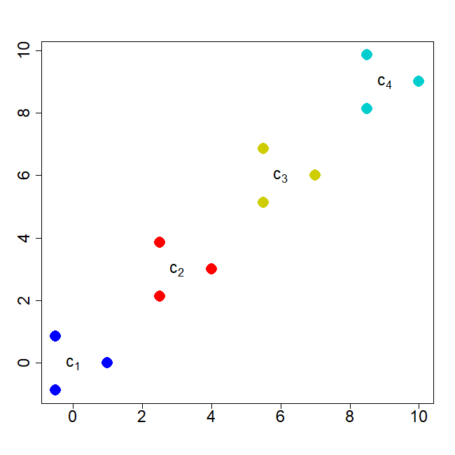
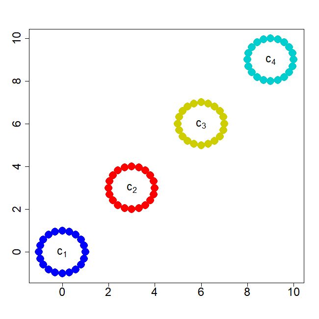
Figure 4: Conditions when $p=12$ (a) and $p=80$ (b). The colors are associated with each group of conditions.

(b) The theoretical regression coefficient functions.

The theoretical coefficient regression function $\beta=(\beta^{(1)},\ldots,\beta^{(p)})$ is defined as follows:

$$\mbox{Groupe 1:}\ \ \beta^{(j)} =0, j=1,\ldots,\kappa,$$

$$\mbox{Groupe 2:}\ \ \beta^{(j)} =\sqrt{2}\sum_{k=1}^{3}\Delta_{k}, j=\kappa+1,\ldots,2\kappa,$$

$$\mbox{Groupe 3:}\ \ \beta^{(j)} =b_{j}\sum_{k=1}^{9}\Delta_{k}, j=2\kappa+1,\ldots,3\kappa,$$

$$\mbox{Groupe 4:}\ \ \beta^{(j)} =-\sqrt{2}\sum_{k=1}^{3}\Delta_{k}, j=3\kappa+1,\ldots,p,$$

where $b_{j}=(-1)^{j}\frac{1+j\text{mod}\kappa}{\kappa}$, the functions $\Delta_{1},\ldots,\Delta_{9}$ denote the set of functions defined by:

$$\Delta_{s}(t)=(1-0.2(10t-s)^{2})_{+},$$

where $(.)_{+}$ is the positive part function. In this setting, only the third group has different coefficient functions.

(c) The predictor and the response variables.

For $j=1,\ldots,p$, $X^{(j)}$ is generated as

$$X^{(j)}(t)=\sum_{s=1}^{9}a_{s}\Delta_{s}(t),$$

where $a_{s}\sim\mathscr{N}(0,1),s=1,\ldots,9$ and $t\in[0,1]$.
The response variable $Y$ is given by

$$Y=\langle X,\beta\rangle_{\mathscr{H}}+\epsilon,$$

where $\epsilon\sim\mathscr{N}(0,\sigma^{2}_{\epsilon})$. The values of $\sigma^{2}_{\epsilon}$ are set such that the noise to signal ratio, $\displaystyle\frac{\sigma^{2}_{\epsilon}}{var(Y)}$, is of about $10\%$.

(d) The two simulation settings

Two scenarios are presented according to the size of groups, $\kappa$:

• $\kappa=3$, $\sigma_{\epsilon}=1.6$

• $\kappa=20$, $\sigma_{\epsilon}=3.6$

The theoretical coefficient regression functions $\beta^{(j)}$, $j=1,\ldots,p$ for the two scenario are presented in Figure 5.

		Group 1 ${\scriptstyle\beta^{(1)}=\beta^{(2)}=\beta^{(3)}}$	Group 2 ${\scriptstyle\beta^{(4)}=\beta^{(5)}=\beta^{(6)}}$	Group 3 ${\scriptstyle\beta^{(7)}\neq\beta^{(8)}\neq\beta^{(9)}}$	Group 4 ${\scriptstyle\beta^{(10)}=\beta^{(11)}=\beta^{(12)}}$
S1	$\beta^{(j)}\mbox{'s}$
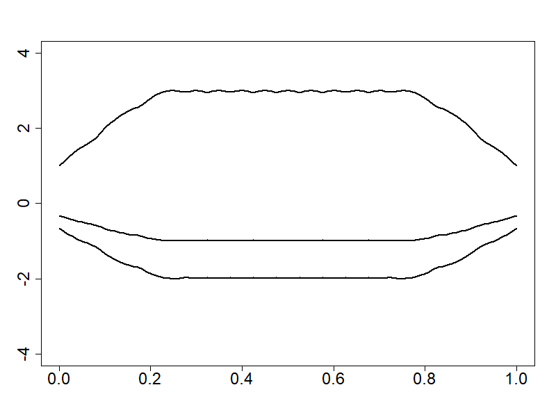
		${\scriptstyle\beta^{(1)}=\beta^{(2)}=\ldots=\beta^{(20)}}$	${\scriptstyle\beta^{(21)}=\beta^{(22)}=\ldots=\beta^{(40)}}$	${\scriptstyle\beta^{(41)}\neq\beta^{(42)}\neq\ldots\neq\beta^{(60)}}$	${\scriptstyle\beta^{(61)}=\beta^{(62)}=\ldots=\beta^{(80)}}$
S2	$\beta^{(j)}\mbox{'s}$

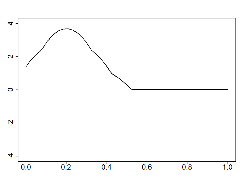
Figure 5: Theoretical regression coefficient function $\beta$ for the two scenario

The function predictor $\bf X$ is observed on $100$ equidistant sampling time points in the interval $[0,1]$. For all dimensions of $\bf X$, $X^{(j)}$ $j=1,\ldots,p$, we use as an approximation their expansion into a cubic B-splines basis of size $M=20$. To assess model performances, a random training sample of $80\%$ of the data is considered and the remaining $20\%$ is used for prediction. This experiment is repeated $I=100$ times.

(e) The competitor methods

The variable fusion methodology (FU) is employed using the 1-NN relationship among conditions whereas the grouping structure is used for the group fusion lasso (GFUL). In order to evaluate their performances, FU and GFUL are compared with two group lasso methods (Godwin, , 2013). The first one, denoted by GL1 (”Group Lasso 1”), uses each dimension $X^{(j)}$ of ${\bf X}$ as a group, as in the classical lasso setting. The second one, denoted by GL2 (Group Lasso 2), uses the same group definitions as in GFUL (see equation (8) ).
In addition to these methods, we propose also the regression model HG (Homogeneous Groups) resuming all the conditions within a group $\mathscr{I}_{k}$ by their mean function,

$$m^{(k)}=\frac{1}{p_{k}}\sum_{j\in\mathscr{I}_{k}}X^{(j)},$$

and then fit a multivariate functional linear model

$$Y=\sum_{k=1}^{K}\int_{0}^{T}m^{(k)}(t)\gamma^{(k)}(t)dt+\epsilon,$$

using principal component regression methodology (Aguilera et al., (2006)).
The idea behind this method is to obtain the same coefficient regression function for all conditions within a group, and that for all the groups: $\forall k=1,\ldots,K$,

$$\beta^{(j)}=(1/p_{k})\gamma^{(k)},\ \ \ \forall j\in\mathscr{I}_{k}.$$

The difference with GFUL is that the latter one allows only for some groups to have identical coefficient functions, whereas HG imposes it for all groups.

Except for the model HG which doesn’t have a penalty term, the hyperparameters ($\alpha,\lambda$) in (10)) are tuned by 10-fold cross-validation: $\lambda$ is chosen from the set

$$\lambda\in\left\{0.96^{i}\lambda_{\max},i=0,1,\ldots,148\right\}\cup\left\{0\right\}$$

and

$$\alpha\in\{0.1,0.2,\ldots,1\},$$

with $\lambda_{\max}$ is determined as in Lukas and Meier, (2020).

(f) The goodness of fit and homogeneity among conditions coefficient regression functions

For each method, the goodness of fit is assessed by the mean squared error (MSE) computed on the test set. Their ability to recover the true equality among coefficient functions $\beta^{(j)}$ is measured by ”sensitivity” (Sens) and ”specificity” (Spec) metrics. They are defined as follows. For each pair $\left(\beta^{(j)},\beta^{(k)}\right)$, $j,k=1,\ldots,p$, we define

$$Sens(j,k)=\mathbb{P}\left(\hat{\beta}^{(j)}=\hat{\beta}^{(k)}|\beta^{(j)}=\beta^{(k)}\right),$$

and

$$Spec(j,k)=\mathbb{P}\left(\hat{\beta}^{(j)}\neq\hat{\beta}^{(k)}|\beta^{(j)}\neq\beta^{(k)}\right).$$

Thus, $Sens(j,k)$ measures the capability of the method to obtain identical estimated coefficient functions $\hat{\beta}^{(j)}=\hat{\beta}^{(k)}$ when the theoretical ones verify that equality, $\beta^{(j)}=\beta^{(k)}$.

Then, as global measures, let define

Sens $$=\frac{2}{p(p-1)}\sum_{j=1}^{p}\sum_{k<j}Sens(j,k),$$

Spec $$=\frac{2}{p(p-1)}\sum_{j=1}^{p}\sum_{k<j}Spec(j,k).$$

3.1.2 Results

Scenario 1

Let remind that in this scenario $p=12$ and $\kappa=3$. The summary of the obtained metrics in S1 is presented Table 1.

In the first scenario ($p=12$), all models give close results except the naive model (HG). Indeed, the HG model gives the highest MSE and the estimation of the coefficient functions is not consistent (see Figure 6). Thus, the naive hypothesis that ” dimensions in the same group share the same regression coefficient function” might lead to inconsistent results. Table 1 shows that the variable fusion (FU) and the group fusion lasso methods (GFUL) reach the highest scores of sensibility and specificity. This demonstrates the ability of these methodologies to find true equalities among coefficients as compared to the group lasso methods (GL1 and GL2).

	MSE	Sens	Spec
GL1	6.2(1.59)	0.22(0.13)	1(0.01)
GL2	6.07(1.45)	0.29(0.12)	1(0)
FU	5.97(1.52)	0.82(0.22)	0.99(0.01)
GFUL	5.21(1.81)	0.92(0.22)	1(0)
HG	14.85(3.25)	1(0)	0.95(0)

Table 1: Scenario S1: MSE mean and standard error (in parentheses), Sensibility and specificity obtained metrics with $I=100$ experiments.

	Group 1 ${\scriptstyle\beta^{(1)}=\beta^{(2)}=\beta^{(3)}}$	Group 2 ${\scriptstyle\beta^{(4)}=\beta^{(5)}=\beta^{(6)}}$	Group 3 ${\scriptstyle\beta^{(7)}\neq\beta^{(8)}\neq\beta^{(9)}}$	Group 4 ${\scriptstyle\beta^{(10)}=\beta^{(11)}=\beta^{(12)}}$
GFUL
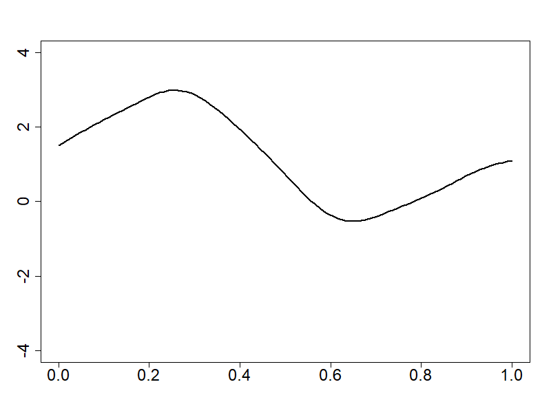
FU
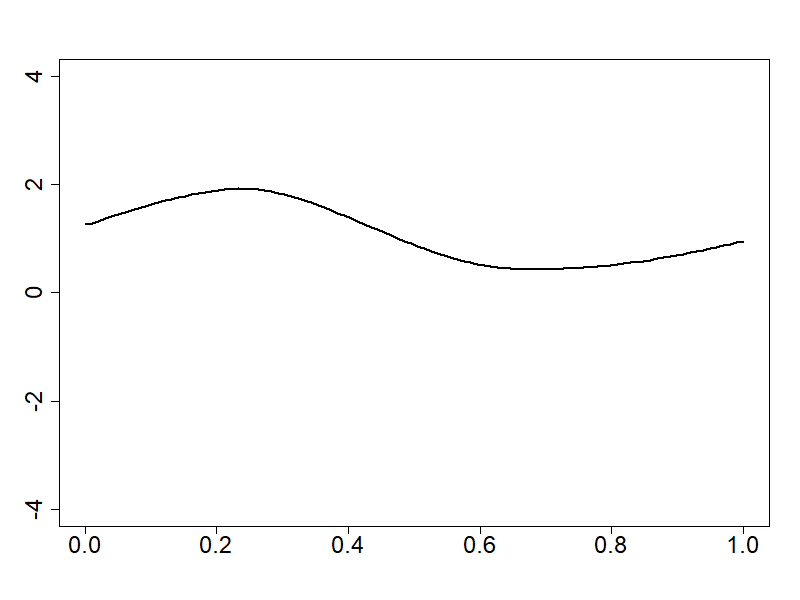
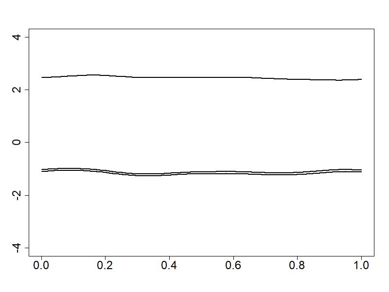
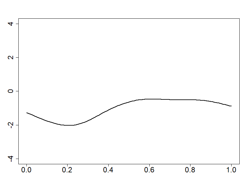
GL1
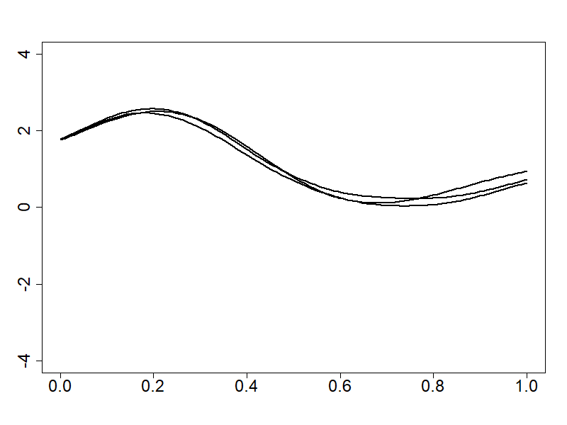
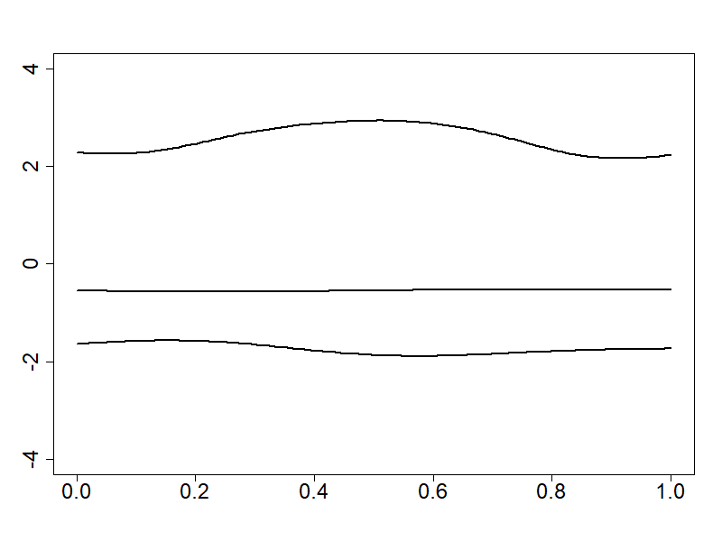
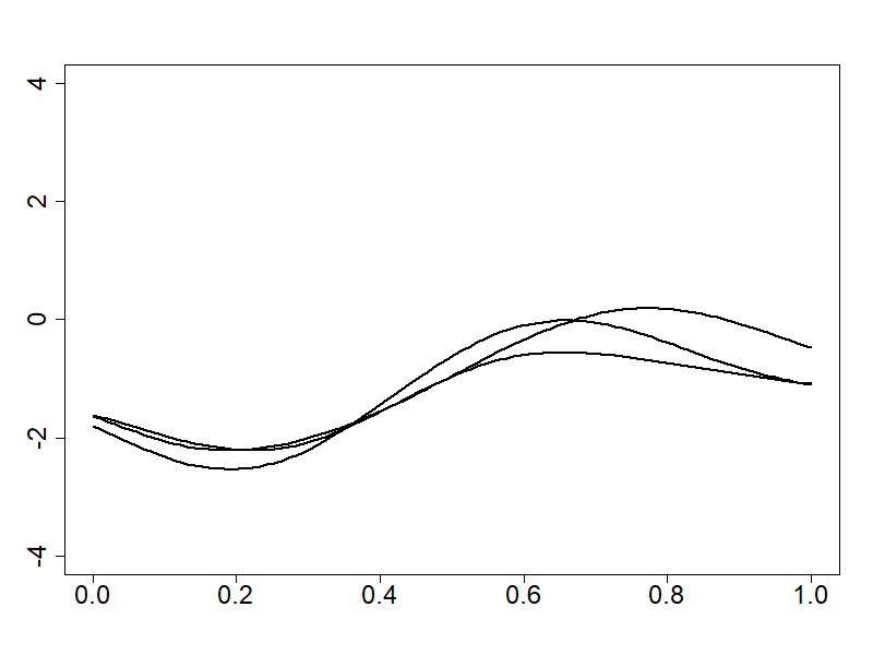
GL2
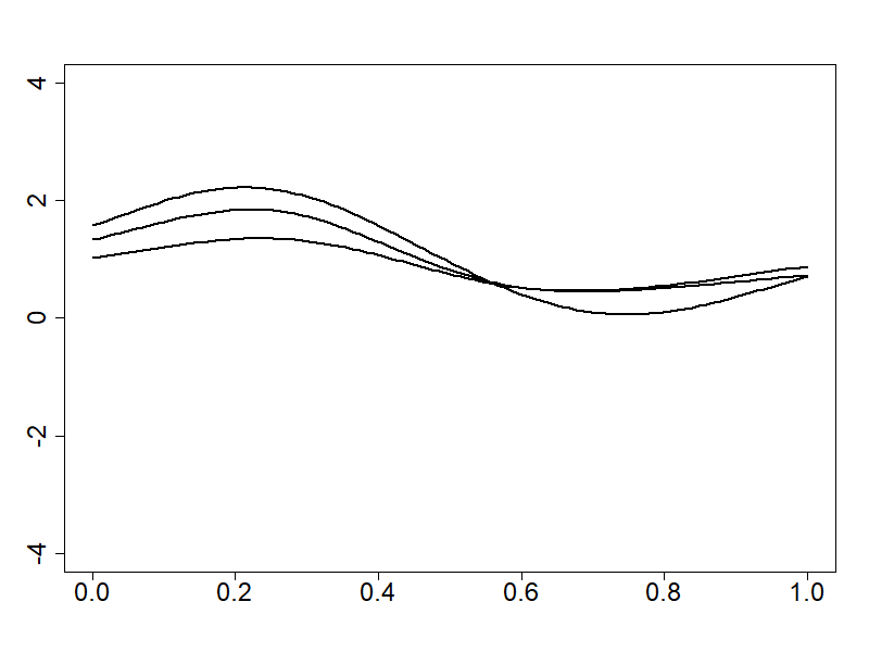
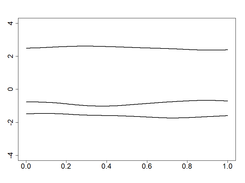
HG

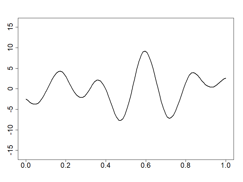
Figure 6: Scenario 1- The estimations of $\beta$ by the different methods(first simulation).

Scenario 2:

In this scenario, $p=80$ and $\kappa=20$. Table 2 presents the results. It shows that GFUL is the best methodology for the MSE metric. The high specificity and the low sensitivity of the competitor methods indicate that they ignore that some groups share the same regression coefficient functions (see Figure 7). This is also reflected in the MSE criteria.

Let observe that all the other methods, including FU, provide quite bad results with respect to GFUL. This can be explained by the fact that these methods are clearly not adapted to consider the grouping structure of conditions.

	MSE	Sens	Spec
GL1	88.74(23.75)	0.2(0.19)	0.85(0.18)
GL2	64.29(17.22)	0.08(0.14)	1(0)
FU	70.58(18.53)	0.07(0.01)	1(0)
GFUL	31.68(16.33)	0.73(0.4)	1(0)
HG	69.37(15.61)	1(0)	0.93(0)

Table 2: Scenario S2: MSE mean and standard error (in parentheses), Sensibility and specificity obtained metrics with $I=100$ experiments.

	Group 1 ${\scriptstyle\beta^{(1)}=\beta^{(2)}=\ldots=\beta^{(20)}}$	Group 2 ${\scriptstyle\beta^{(21)}=\beta^{(22)}=\ldots=\beta^{(40)}}$	Group 3 ${\scriptstyle\beta^{(41)}\neq\beta^{(42)}\neq\ldots\neq\beta^{(60)}}$	Group 4 ${\scriptstyle\beta^{(61)}=\beta^{(62)}=\ldots=\beta^{(80)}}$
GFUL
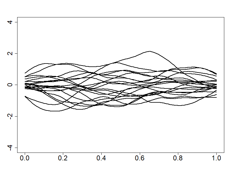
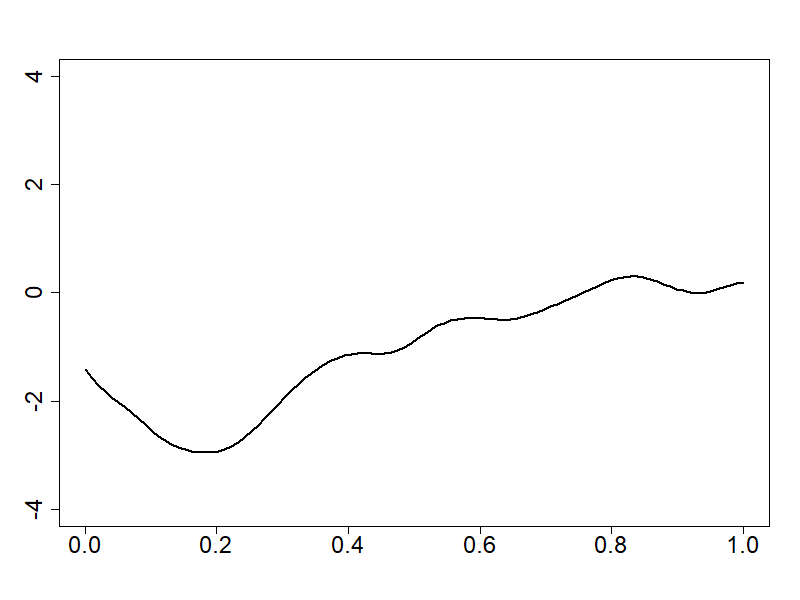
FU
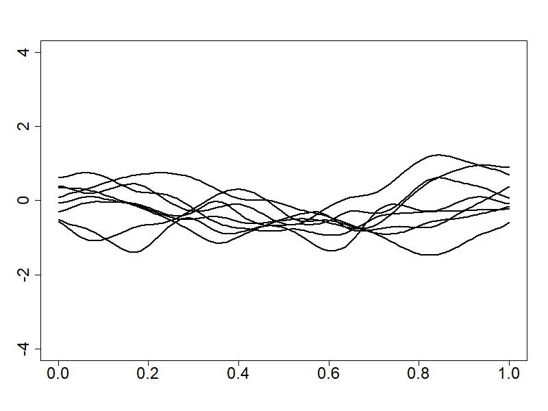
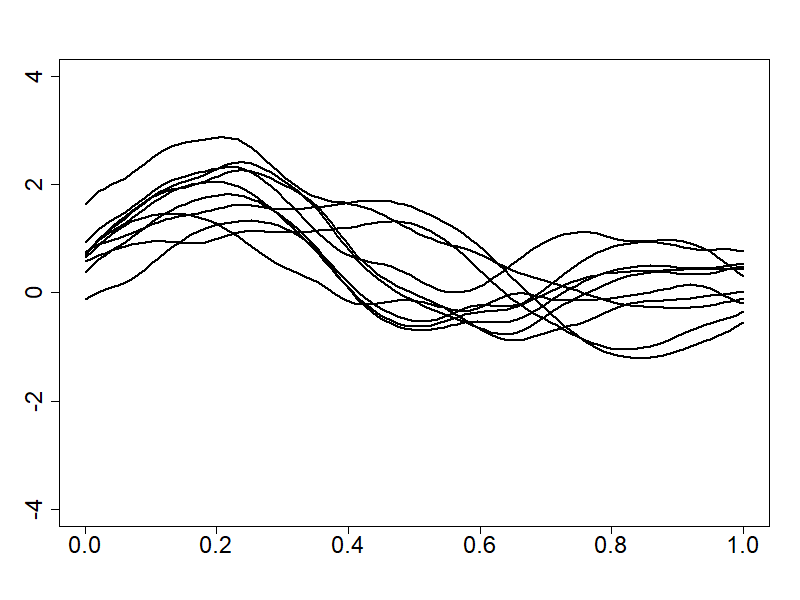
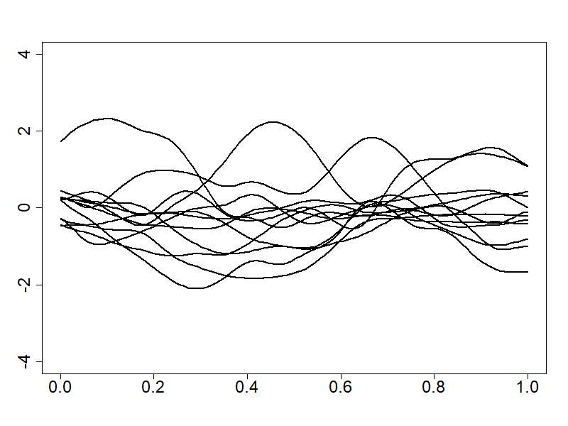
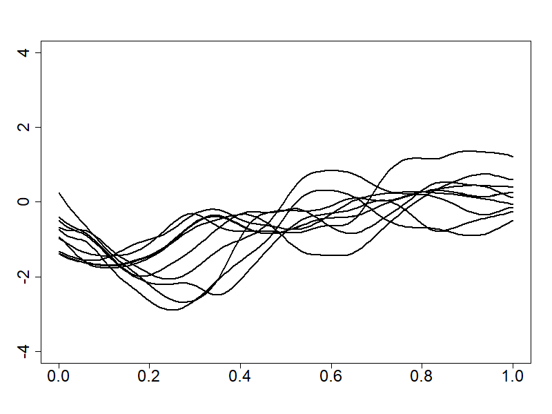
GL1
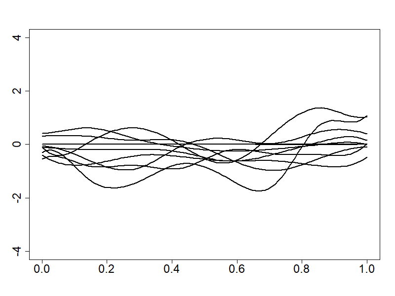
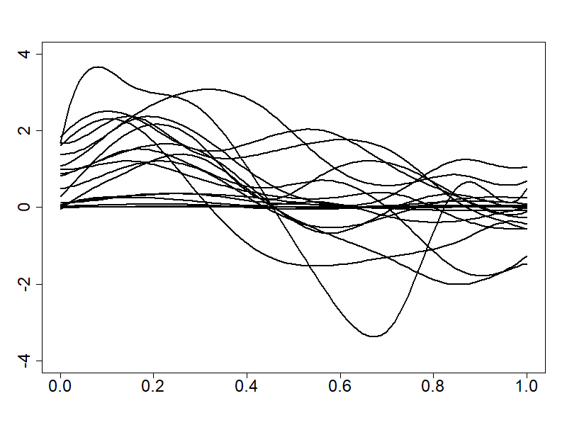
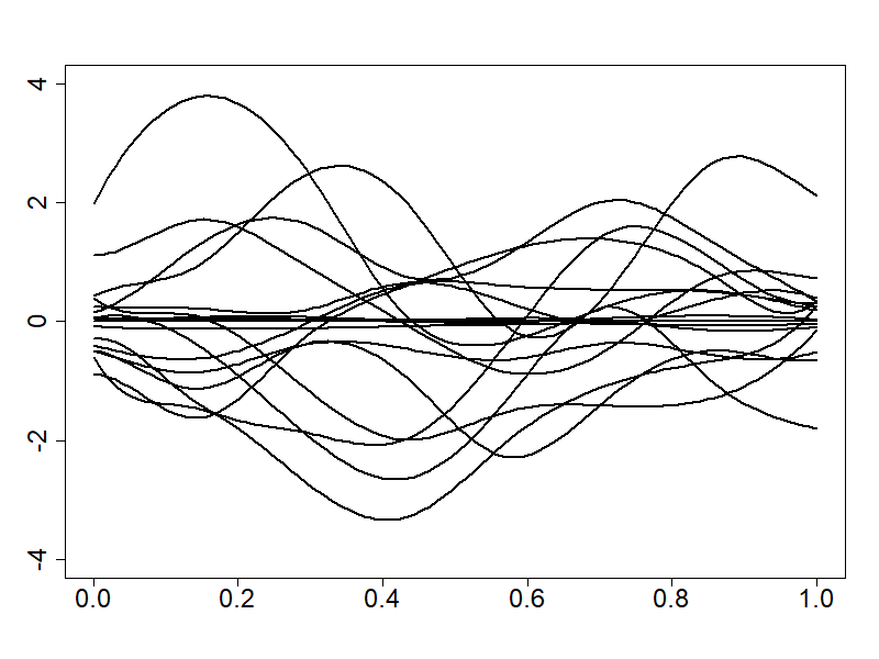
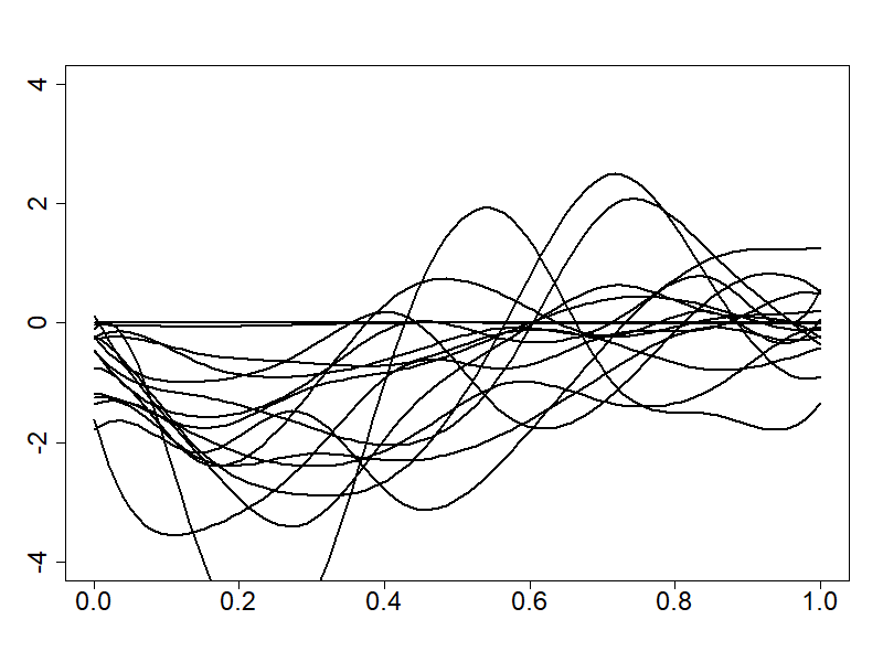
GL2
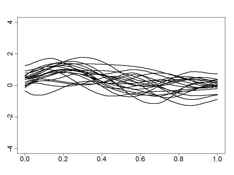
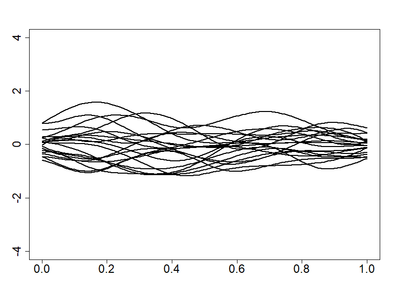
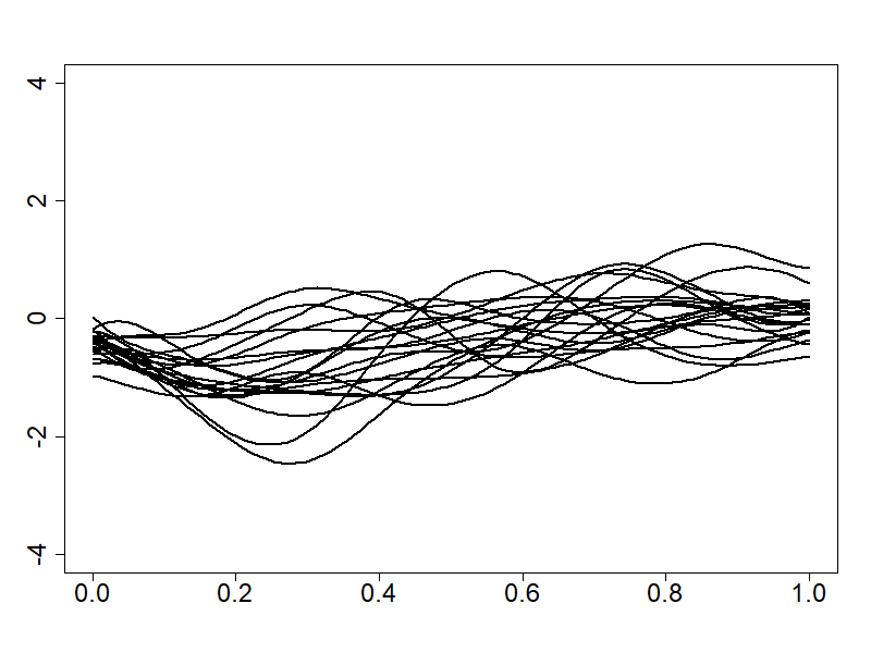
HG

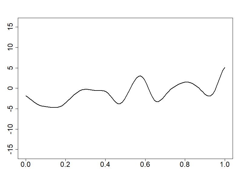
Figure 7: Scenario 2- The estimations of $\beta$ by the different methods (first simulation).

3.2 Application: FingerMovements

In this section, we are interested in a supervised binary classification problem for FingerMovements dataset. These data come from the brain-computer interface domain and are used for binary classification as a benchmark. More precisely, a subject has been asked to type characters using only the index and the pinky fingers of the right ($Y=0$) and the left ($Y=1$) hands. The challenge is to determine, based on their electroencephalography (EEG) recording ($\bf X$), the hand that has been used. The EEG signal is recorded by $p=28$ sensors located on the scalp during $500$ ms. Thus, for any subject, $p=28$ curves are available. Each curve is summarized by $50$ equidistant times points in the interval $[0,500ms]$. The Figure 1 (see the Introduction section) presents the curves registered by a sample of 6 sensors (named F1,F2, F3, F4,O1,O2), for a given subject. The dataset is composed of $N=416$ subjects and it is split into a training set of $n=316$ units and a test set of $100$ units.

This dataset has been used in Ruiz et al., (2021). The authors showed that the Inception Time (IT) model (Ismail Fawaz et al., , 2020) provides the best predictions among the state-of-the-art models.

In this section we compare the results obtained by our methodologies (FU and GFUL) with the competitors one, i.e. GL1, GL2 and IT.

The FU method is based on the 1-NN graph built with the Euclidean distance between the spatial location of sensors $\mathscr{C}_{j}\in\mathbb{R}^{3}$, $j=1,\ldots,28$. For the GFUL method, we used $K=10$ clusters of conditions obtained from the k-means clustering algorithm applied to sensor locations. The $K=10$ groups correspond to well-defined scalp regions (group $1$ = frontal left, group $2$ = frontal right, etc). See Figure 8.

Conditions	1-NN	Groups

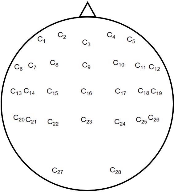
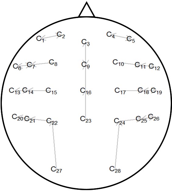
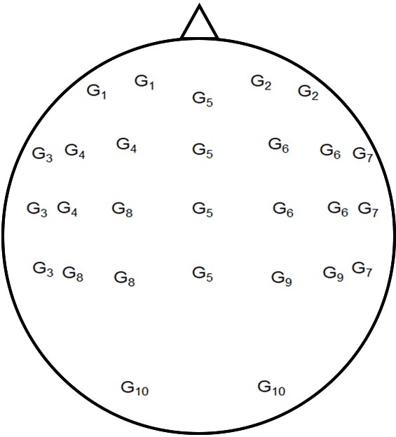
Figure 8: Conditions and groups for the FingerMovements Dataset

Two group lasso models are also fitted: GL1 and GL2. Similarly to the simulation study, the GL1 method uses each dimension as a group whereas GL2 uses the same grouping structure as GFUL.

For all dimensions $X^{(j)}$, $j=1,\ldots,28$, a basis of $M=30$ B-splines is used to reconstruct the functional form of the predictors. The hyperparameters $\lambda$ and $\alpha$ are tuned by a 10-fold cross-validation procedure, on the following grids

$$\lambda\in\left\{0.96^{i}\lambda_{\max},i=0,1,\ldots,148\right\}\cup\left\{0\right\}$$

and

$$\alpha\in\{0,0.1,0.2,\ldots,1\},$$

where $\lambda_{\max}$ is the minimum value such that the penalty term vanishes ($\mathscr{P}(\hat{\beta}_{\lambda,\alpha})=0$).

3.3 Results

FU	GFUL

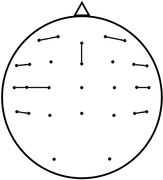
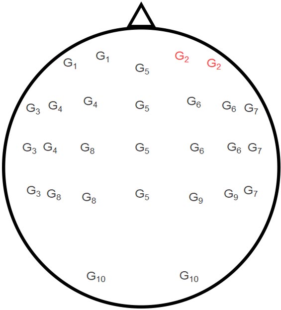
Figure 9: Estimated structures

FU: connected points share the same coefficients, GFUL: groups in red share the same coefficients

Table 3 shows that our proposed methodologies perform better than most competitors (GL2 and IT) in terms of accuracy (well-classified rate) estimated on the test sample. Figure 9 shows the grouping structure of the estimated regression coefficient functions obtained with FU and GFUL. Hence, those results provide information about the importance of sensors and their locations (also through the grouping structure) for the prediction of the response. The associated coefficient functions graphs are presented in the appendix A.

Methods	Accuracy
FU	64%
GFUL	68%
IT	56.7%
GL1	65%
GL2	58%

Table 3: Accuracy obtained on the test dataset

4 Discussion

In this paper we introduced two new criteria for estimating a linear regression model with the predictor represented by a functional random variable observed under different conditions (eventually spatially distributed). We called that data repeated functional. When some grouping structure of the observation conditions is present, our methods can integrate it in the fitting process through specific penalties: fusion and group fusion-lasso.

The numerical simulation study confirms the efficacy of taking into account such a grouping structure of conditions, as well as the application to Finger movements data. Both proposed methodologies give similar results or outperform the lasso method competitors.

The GFUL method can be seen as a generalization of the fusion method in more than one neighbor. However, GFUL tests group membership at once instead of testing one-on-one interactions. This is a quite strong hypothesis, as it assumes that equality relations (among regression coefficient functions) in a group can be either all true or all false. The use of smaller overlaps between groups could be an alternative model. In this setting, the solution is related to the group lasso with overlap, which is more challenging (Yuan et al., , 2011). An extensive study of adapted optimization problems should be done. One can also explore the model group lasso proposed in Jacob et al., (2009). Yet, it seems that using this approach leads to losing the diffusion between overlapped groups, the penalty is no longer defined on the $2,1$ norm (See Jacob et al., (2009) for details). The integration of sparsity conditions and the study of other types of neighborhood structures in the fusion method can be some future promising developments.

Appendix A Additional figures: FingerMovements

$\hat{\beta}^{(1)}=\hat{\beta}^{(2)}$	$\hat{\beta}^{(3)}=\hat{\beta}^{(9)}$	$\hat{\beta}^{(4)}=\hat{\beta}^{(5)}$	$\hat{\beta}^{(6)}=\hat{\beta}^{(7)}$
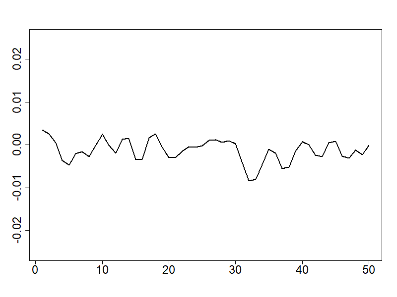
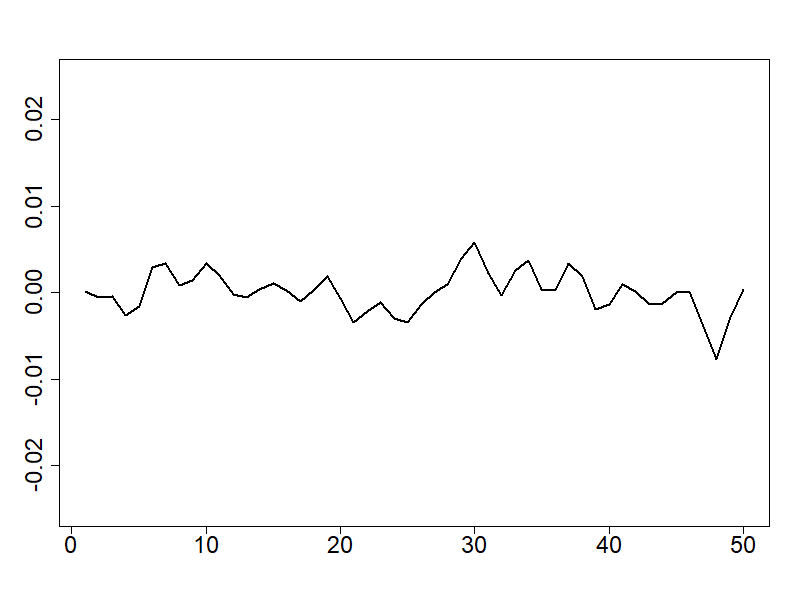
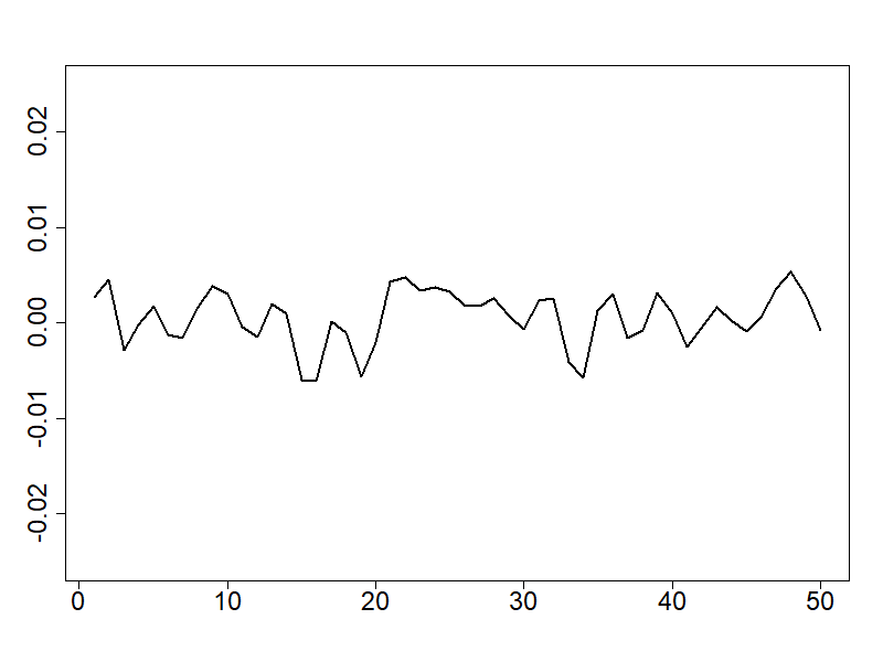
$\hat{\beta}^{(8)}$	$\hat{\beta}^{(10)}$	$\hat{\beta}^{(11)}=\hat{\beta}^{(12)}$	$\hat{\beta}^{(13)}=\hat{\beta}^{(14)}=\hat{\beta}^{(15)}$
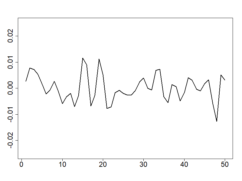
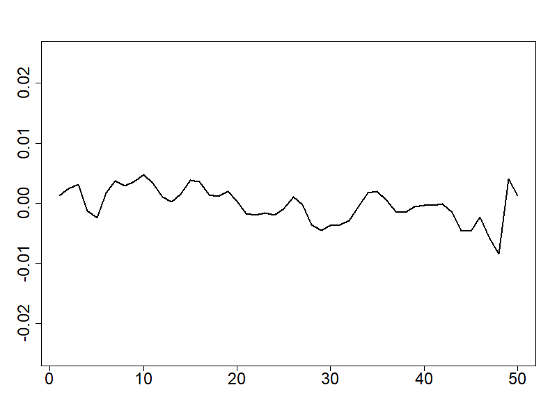
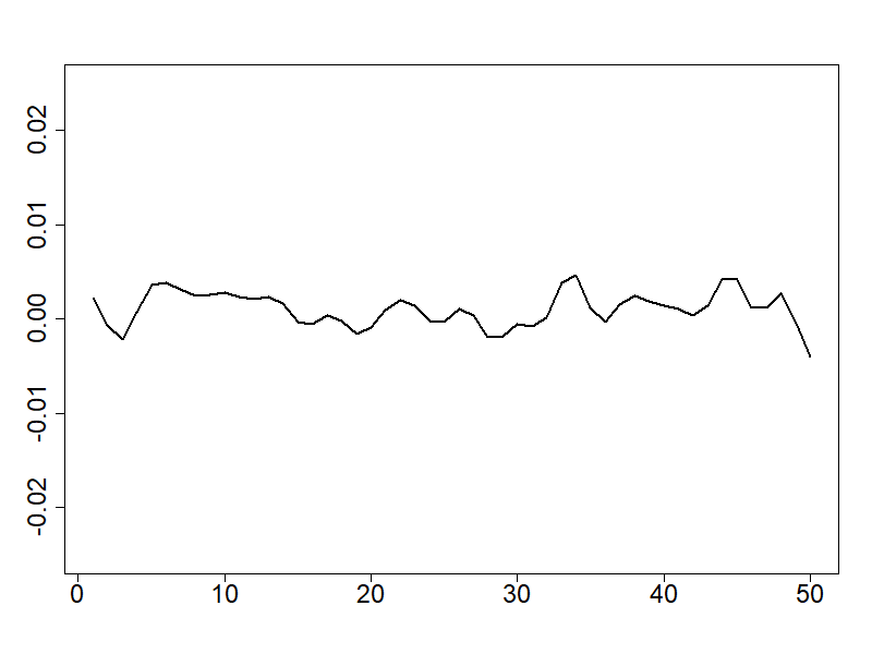
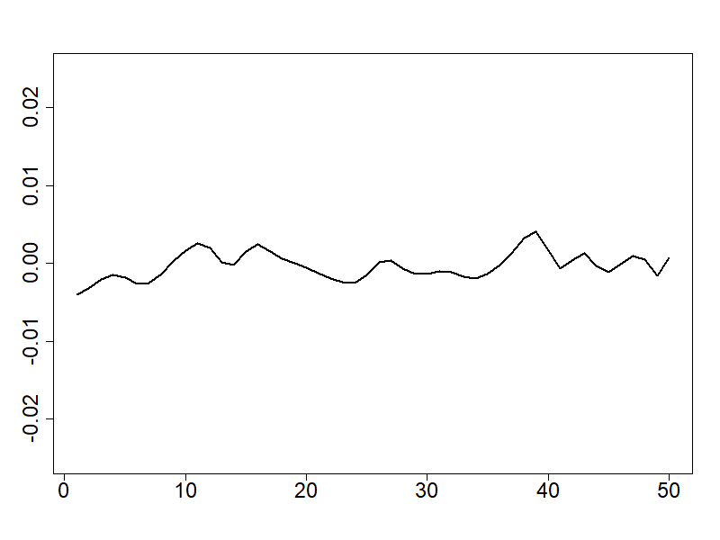
$\hat{\beta}^{(16)}$	$\hat{\beta}^{(17)}$	$\hat{\beta}^{(18)}=\hat{\beta}^{(19)}$	$\hat{\beta}^{(20)}=\hat{\beta}^{(21)}$
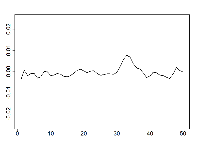
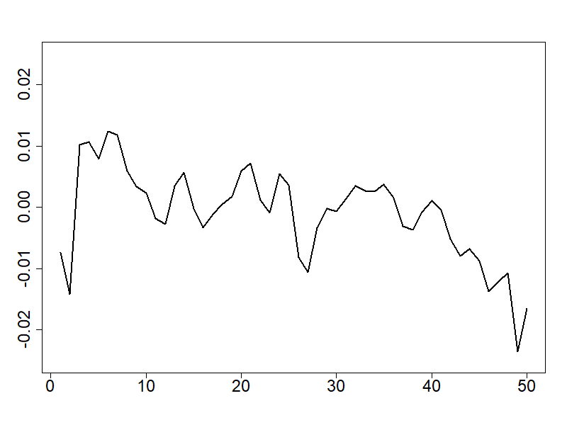
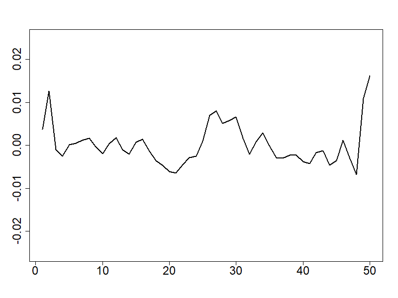
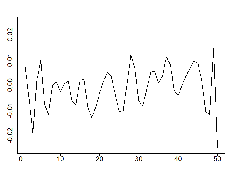
$\hat{\beta}^{(22)}$	$\hat{\beta}^{(23)}$	$\hat{\beta}^{(24)}$	$\hat{\beta}^{(25)}=\hat{\beta}^{(26)}$
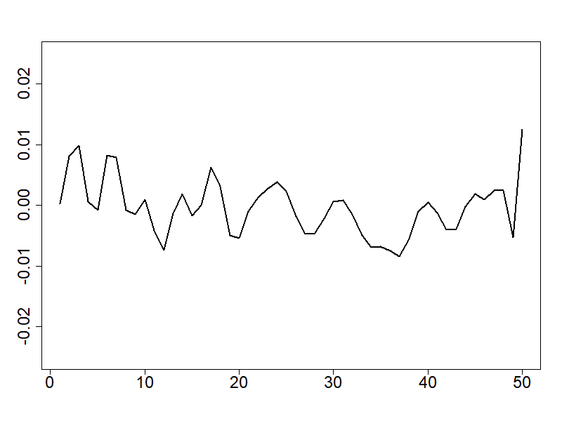
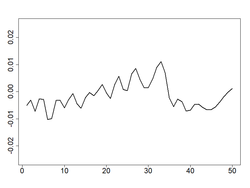
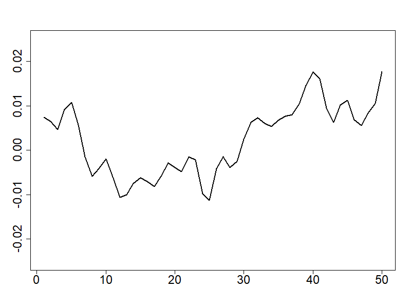
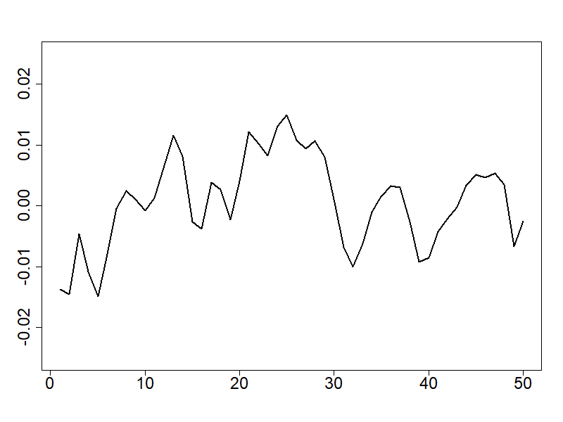
$\hat{\beta}^{(27)}$	$\hat{\beta}^{(28)}$

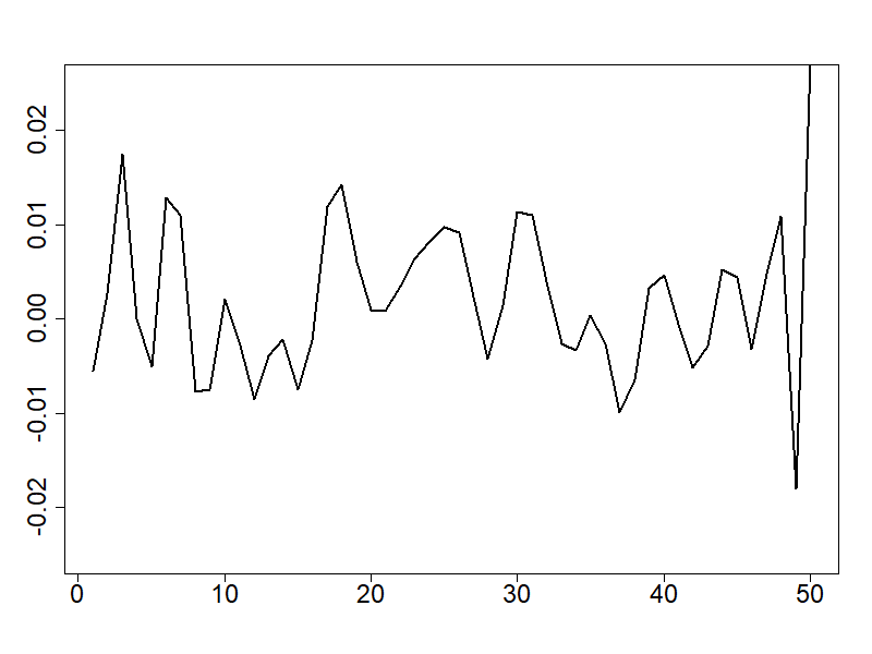
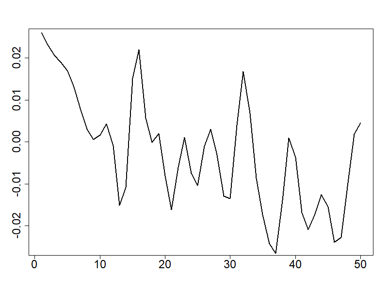
Figure 10: Fusion variable model

Group 1	Group 2	Group 3	Group 4	Group 5
$\scriptstyle\hat{\beta}^{(1)}\neq\hat{\beta}^{(2)}$	$\scriptstyle\hat{\beta}^{(4)}=\hat{\beta}^{(5)}=0$	$\scriptstyle\hat{\beta}^{(6)}\neq\hat{\beta}^{(13)}\neq\hat{\beta}^{(20)}$	$\scriptstyle\hat{\beta}^{(7)}\neq\hat{\beta}^{(8)}\neq\hat{\beta}^{(14)}$	$\scriptstyle\hat{\beta}^{(3)}\neq\hat{\beta}^{(9)}\neq\hat{\beta}^{16)}\neq\hat{\beta}^{(23)}$
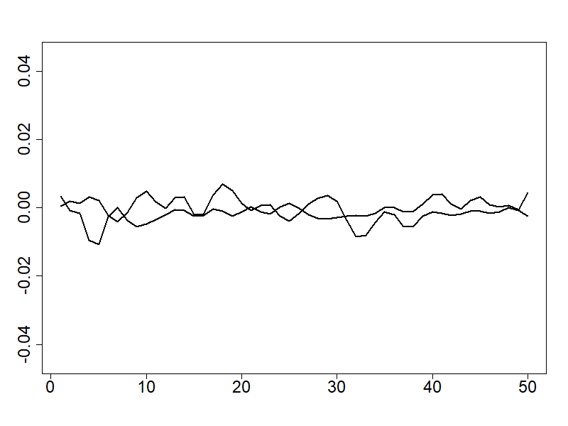
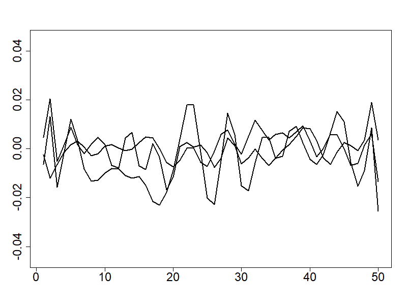
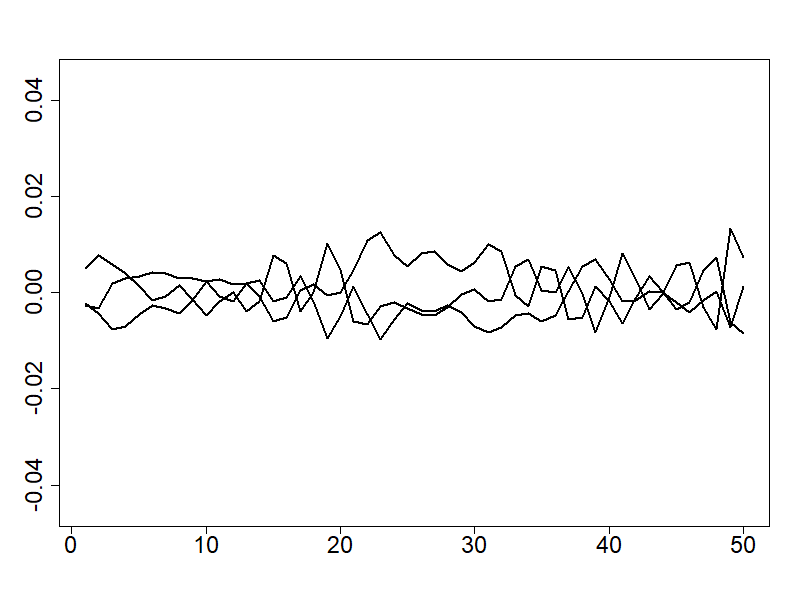
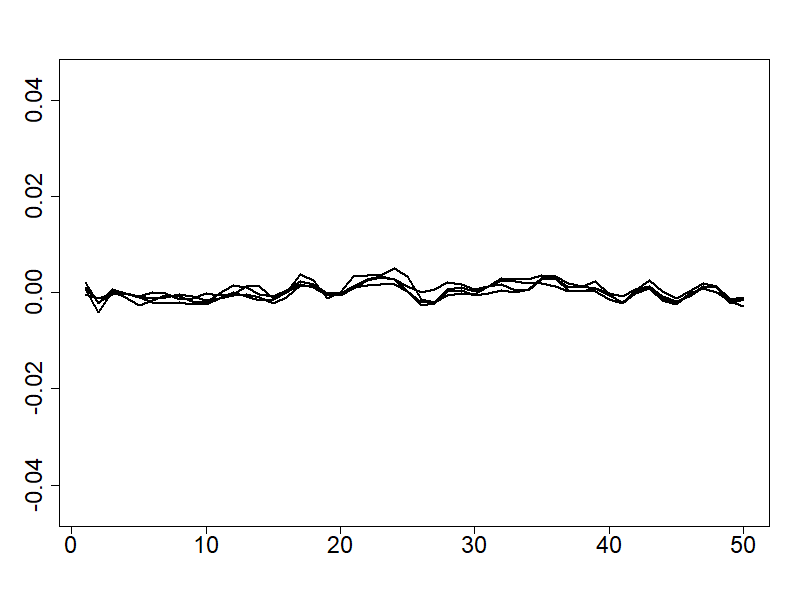
Group 6	Group 7	Group 8	Group 9	Group 10
$\scriptstyle\hat{\beta}^{(10)}\neq\hat{\beta}^{(11)}\neq\hat{\beta}^{(17)}\neq\hat{\beta}^{(18)}$	$\scriptstyle\hat{\beta}^{(12)}\neq\hat{\beta}^{(19)}\neq\hat{\beta}^{(26)}$	$\scriptstyle\hat{\beta}^{(15)}\neq\hat{\beta}^{(21)}\neq\hat{\beta}^{(22)}$	$\scriptstyle\hat{\beta}^{(24)}\neq\hat{\beta}^{(25)}$	$\scriptstyle\hat{\beta}^{(27)}\neq\hat{\beta}^{(28)}$

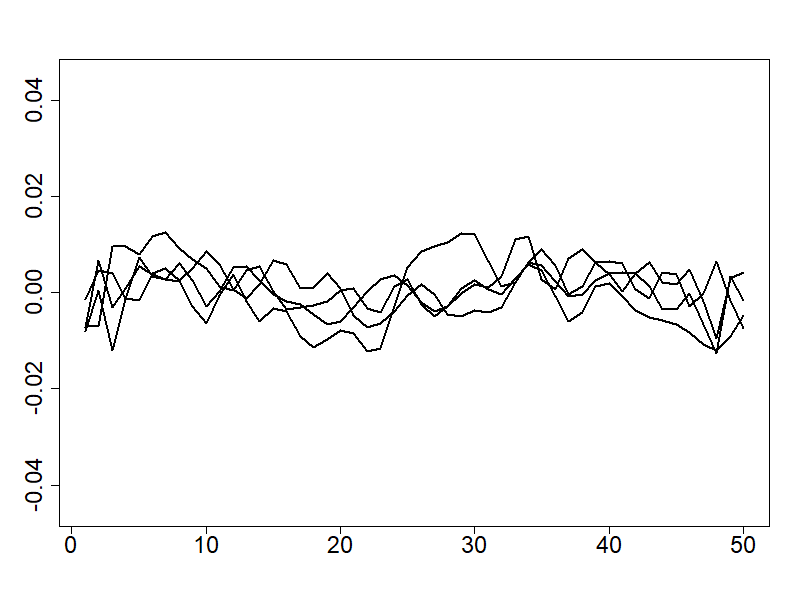
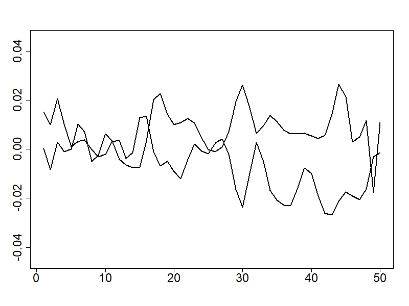
Figure 11: GFUL estimated coefficients

$\hat{\beta}^{(1)}$	$\hat{\beta}^{(2)}$	$\hat{\beta}^{(3)}$	$\hat{\beta}^{(4)}$
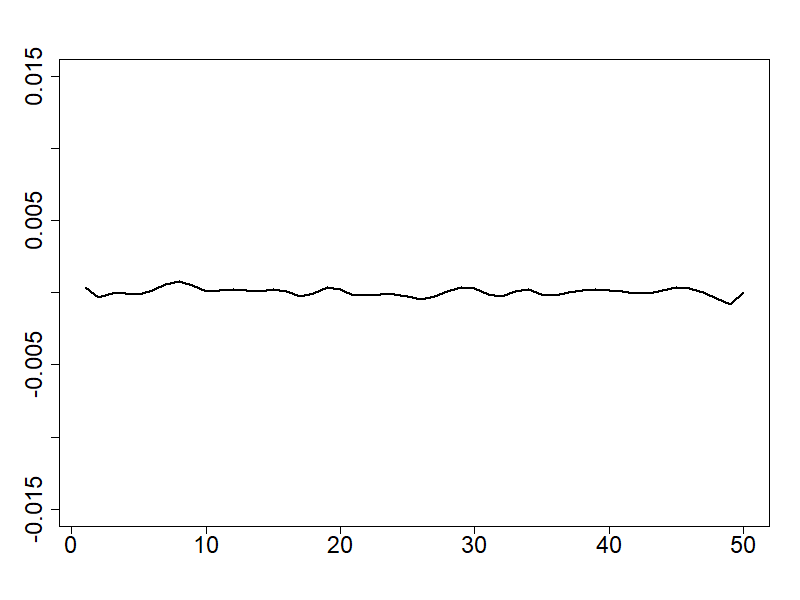
$\hat{\beta}^{(5)}$	$\hat{\beta}^{(6)}$	$\hat{\beta}^{(7)}$	$\hat{\beta}^{(8)}$
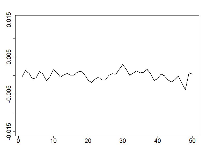
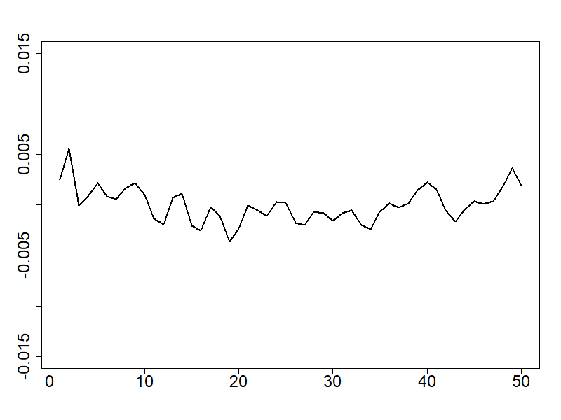
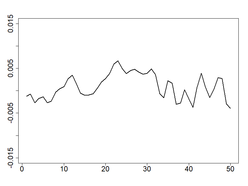
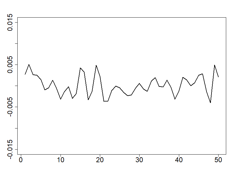
$\hat{\beta}^{(9)}$	$\hat{\beta}^{(10)}$	$\hat{\beta}^{(11)}$	$\hat{\beta}^{(12)}$
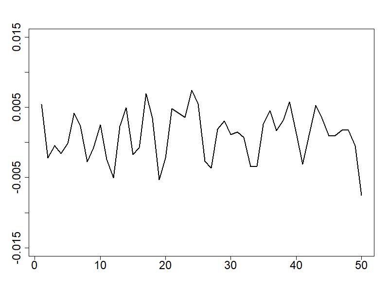
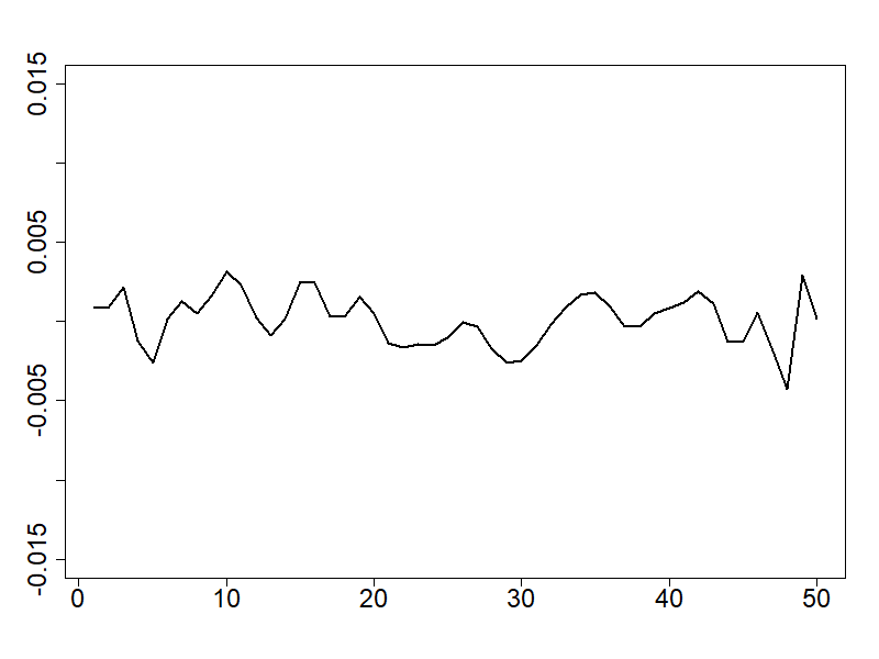
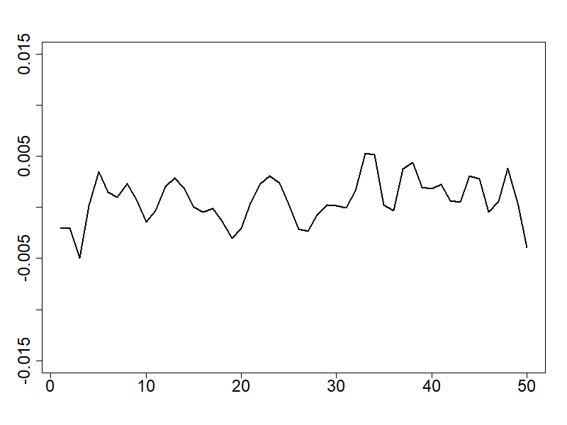
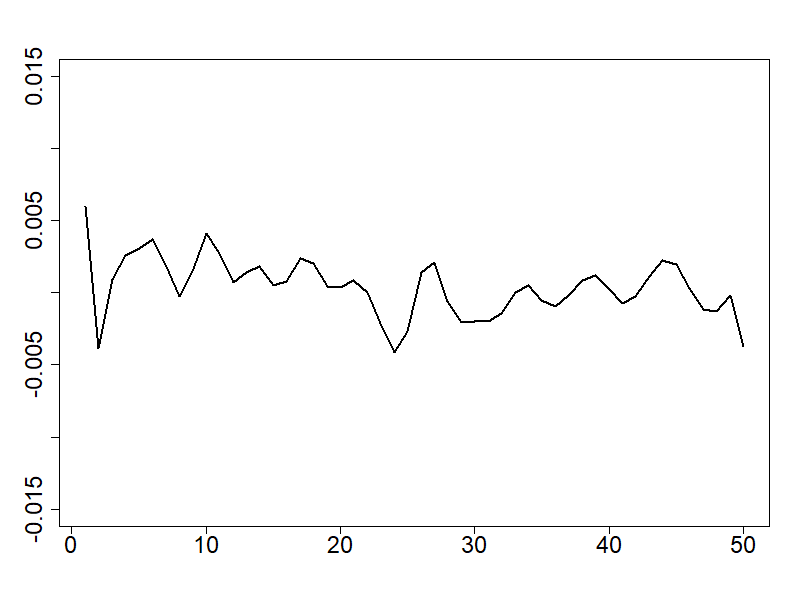
$\hat{\beta}^{(13)}=0$	$\hat{\beta}^{(14)}$	$\hat{\beta}^{(15)}$	$\hat{\beta}^{(16)}$
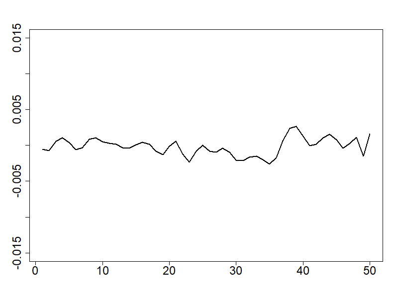
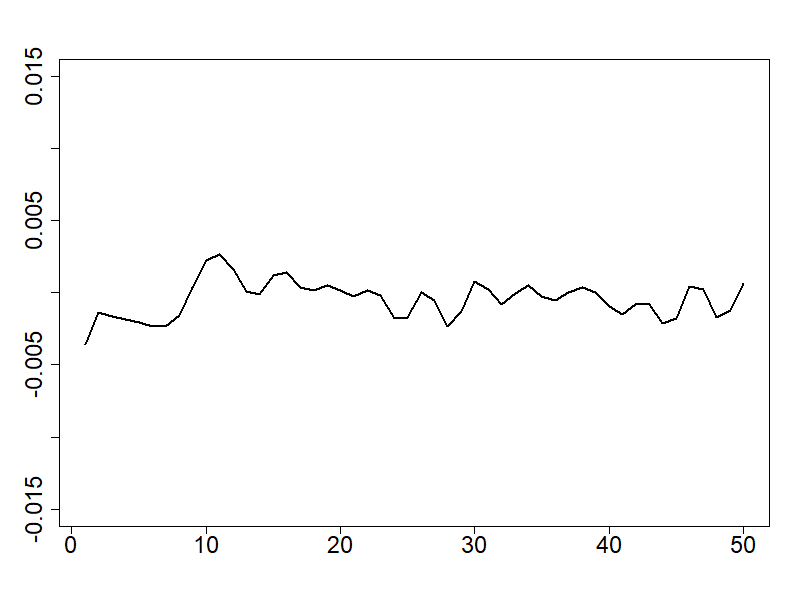
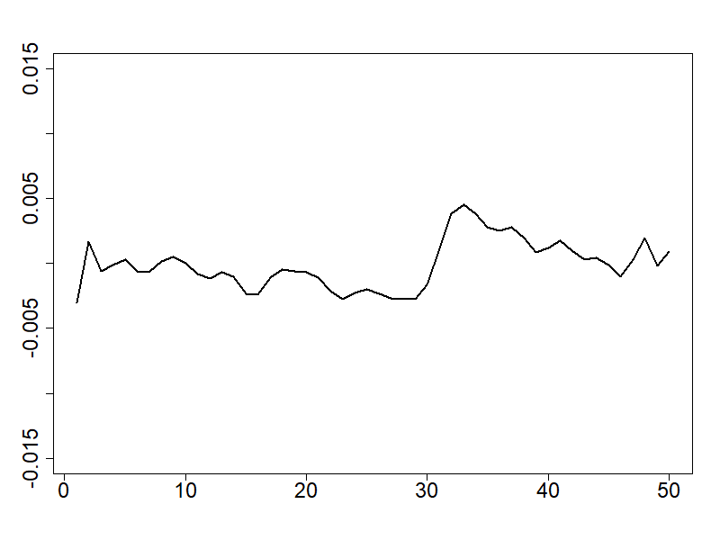
$\hat{\beta}^{(17)}$	$\hat{\beta}^{(18)}$	$\hat{\beta}^{(19)}$	$\hat{\beta}^{(20)}$
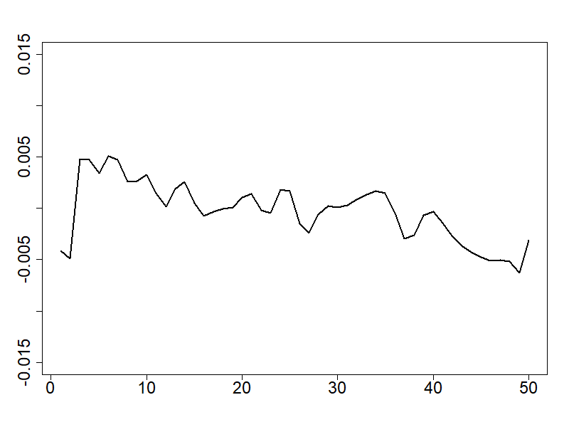
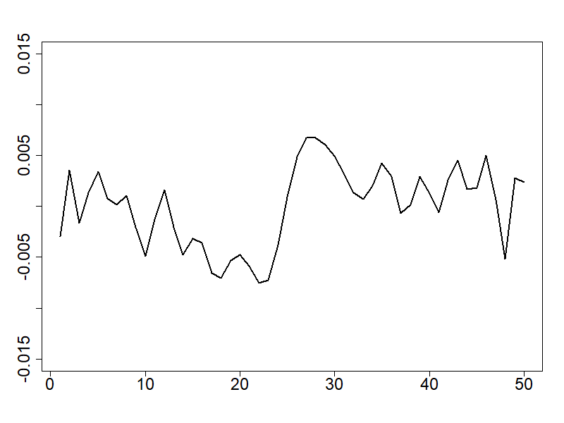
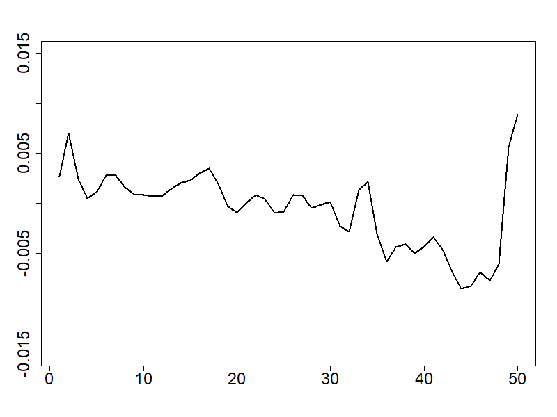
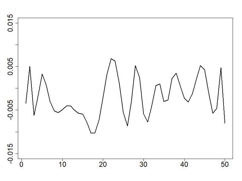
$\hat{\beta}^{(21)}$	$\hat{\beta}^{(22)}$	$\hat{\beta}^{(23)}$	$\hat{\beta}^{(24)}$
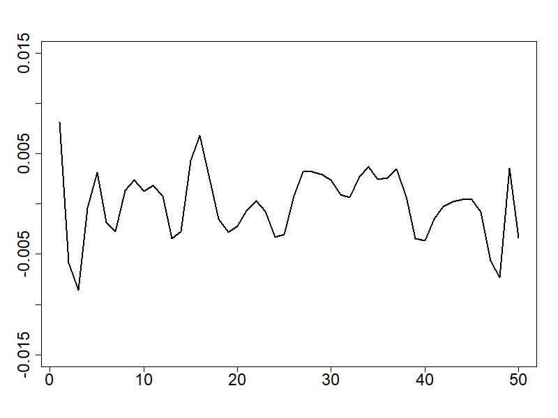
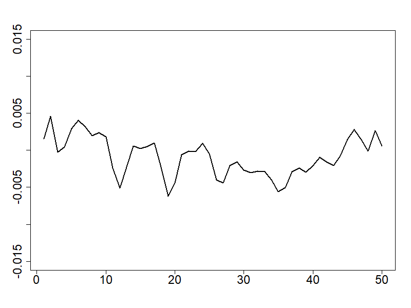
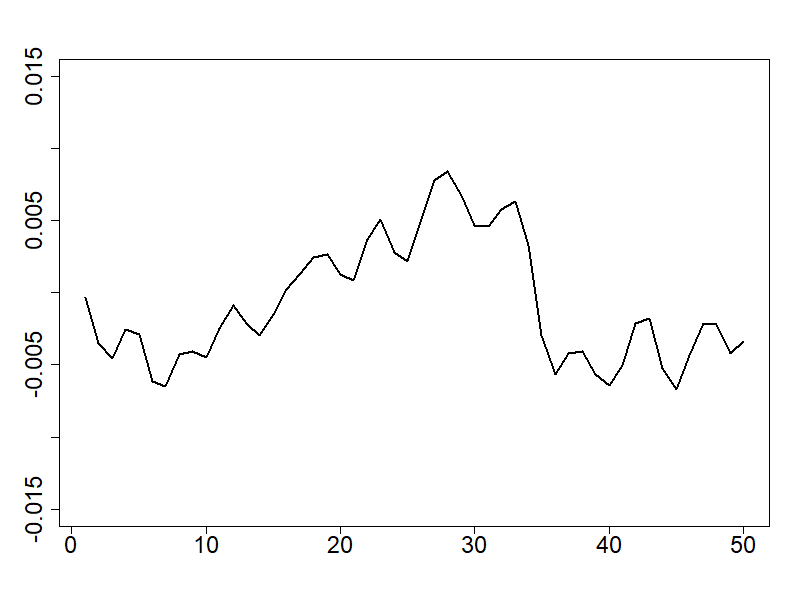
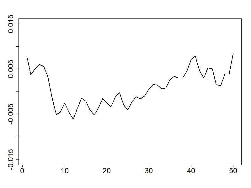
$\hat{\beta}^{(25)}$	$\hat{\beta}^{(26)}$	$\hat{\beta}^{(27)}$	$\hat{\beta}^{(28)}$

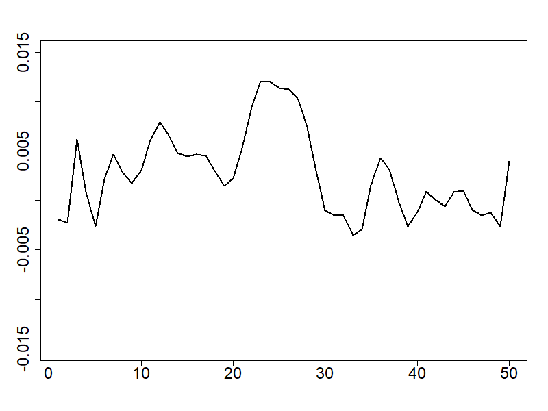
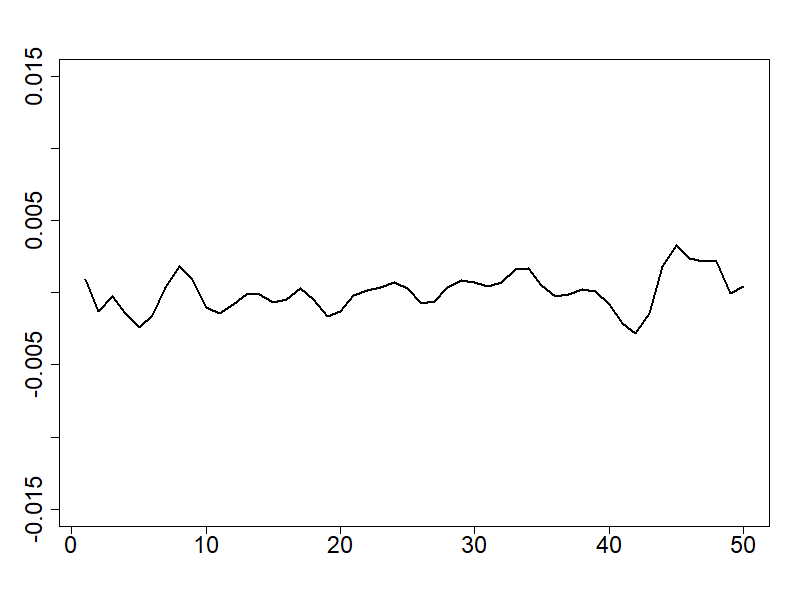
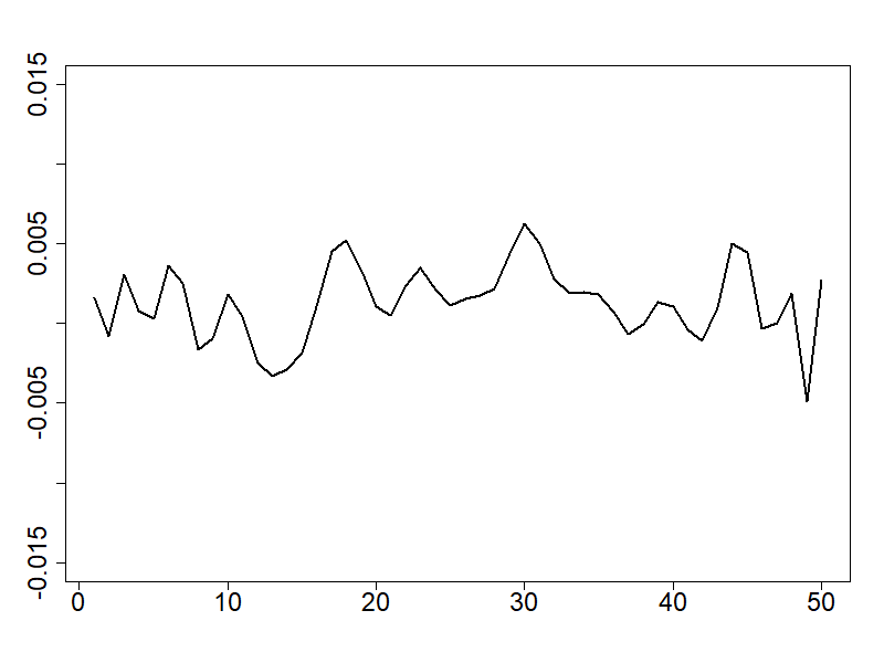
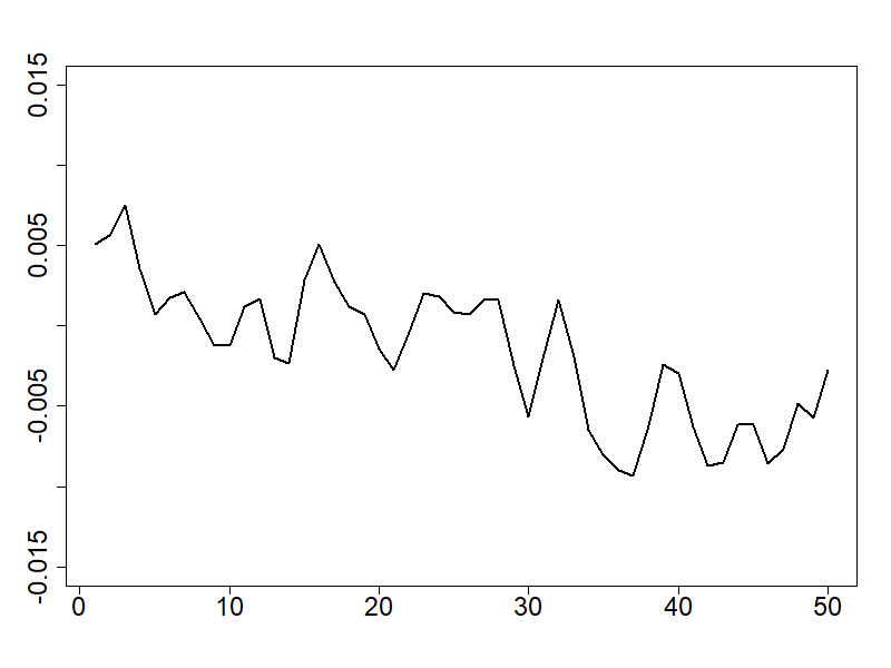
Figure 12: GL1 estimated coefficients model

$\hat{\beta}^{(1)}$	$\hat{\beta}^{(2)}$	$\hat{\beta}^{(3)}$	$\hat{\beta}^{(4)}$
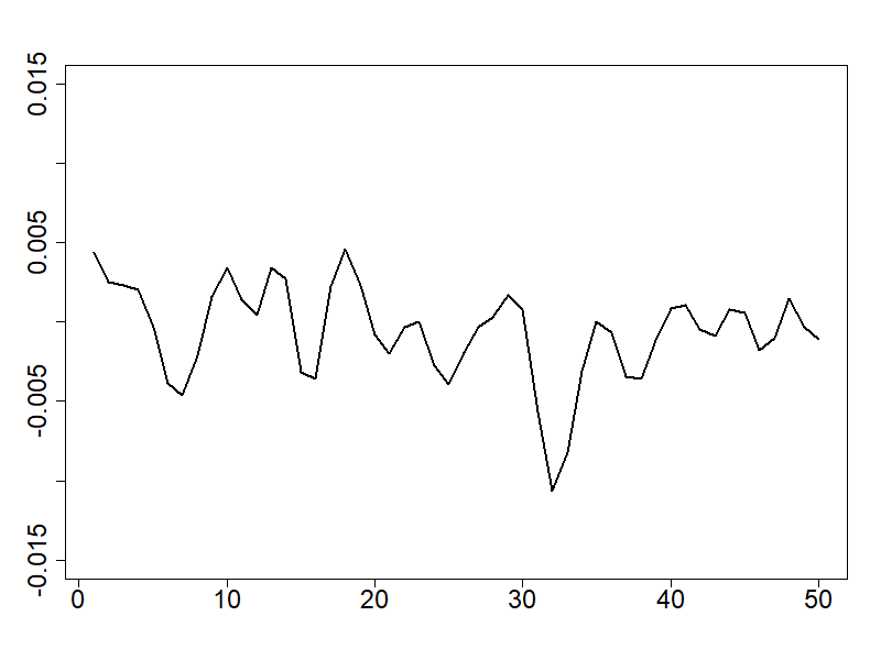
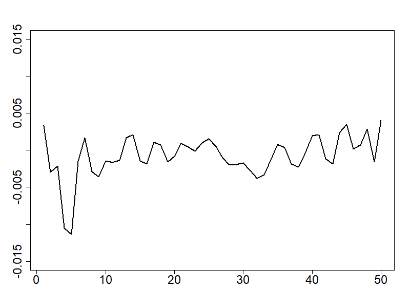
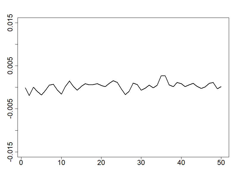
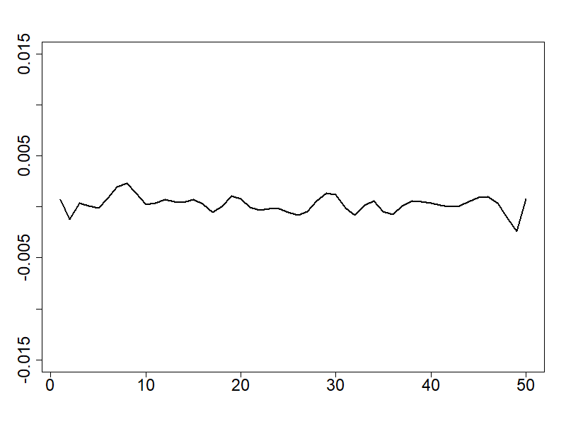
$\hat{\beta}^{(5)}$	$\hat{\beta}^{(6)}$	$\hat{\beta}^{(7)}$	$\hat{\beta}^{(8)}$
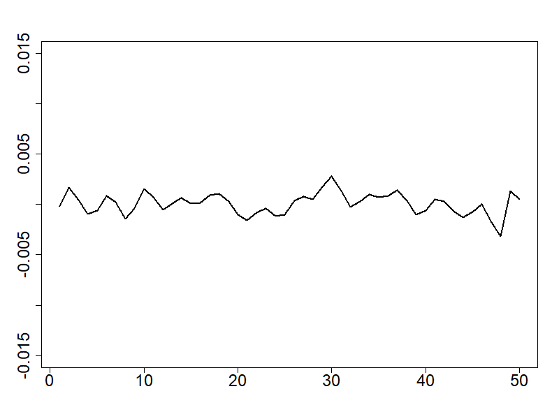
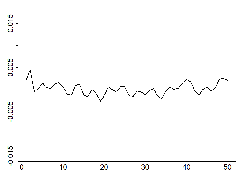
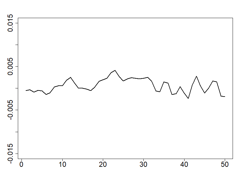
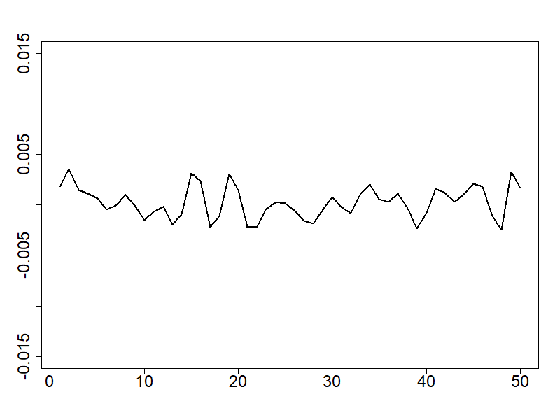
$\hat{\beta}^{(9)}$	$\hat{\beta}^{(10)}$	$\hat{\beta}^{(11)}$	$\hat{\beta}^{(12)}$
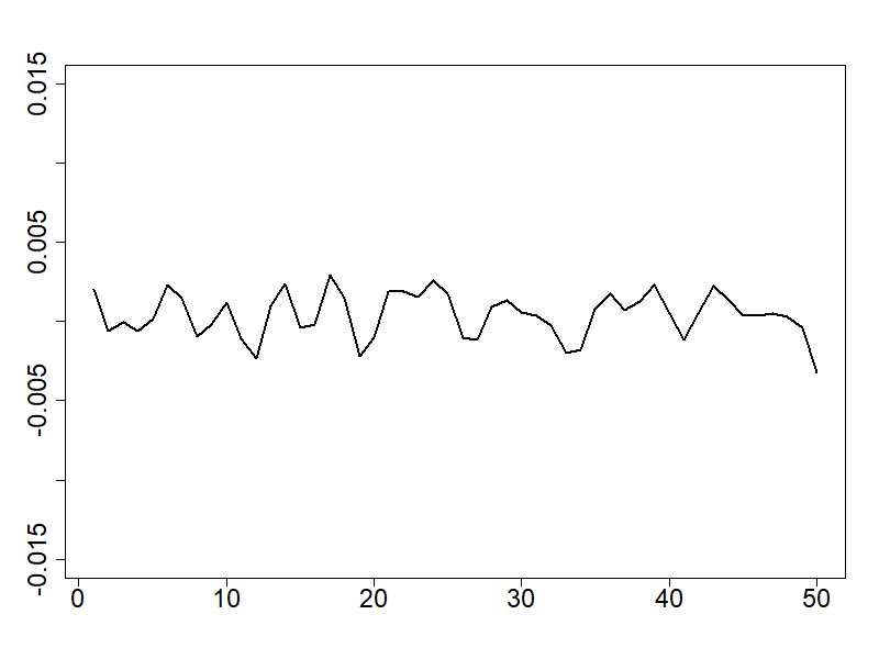
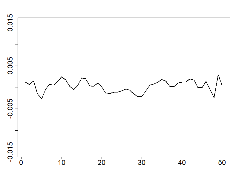
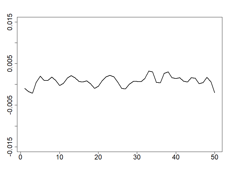
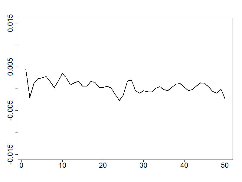
$\hat{\beta}^{(13)}$	$\hat{\beta}^{(14)}$	$\hat{\beta}^{(15)}$	$\hat{\beta}^{(16)}$
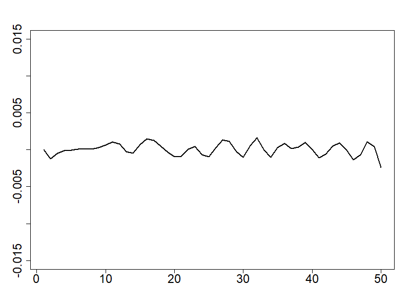
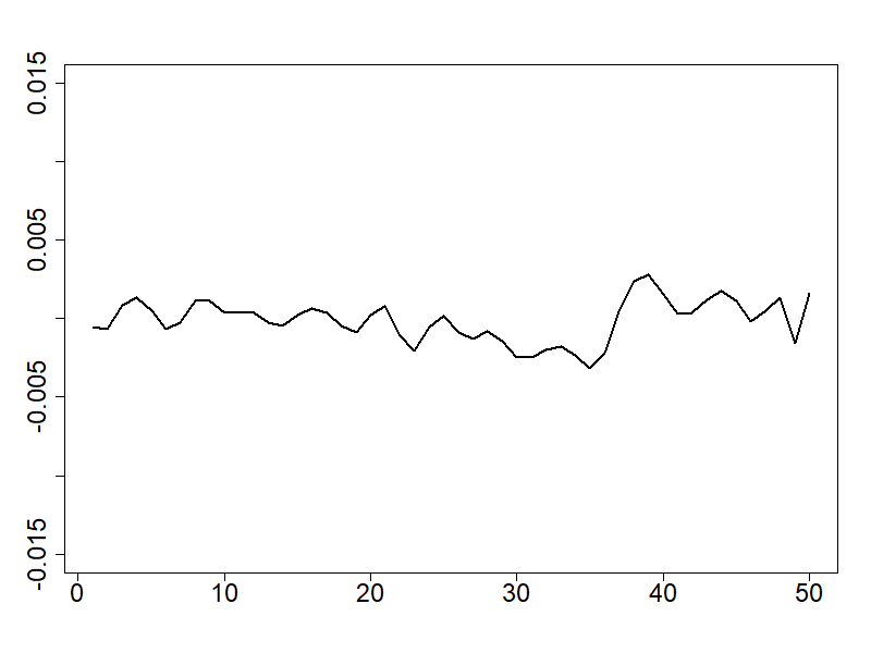
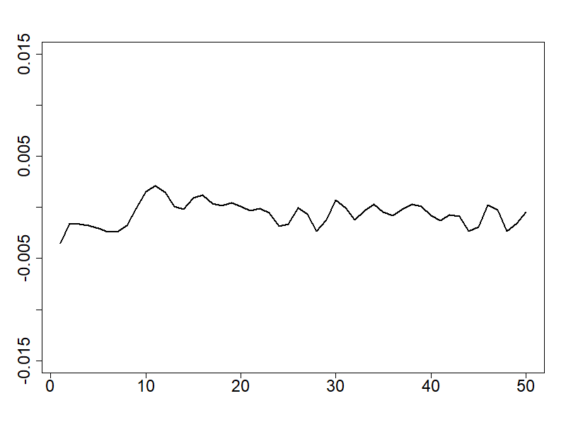
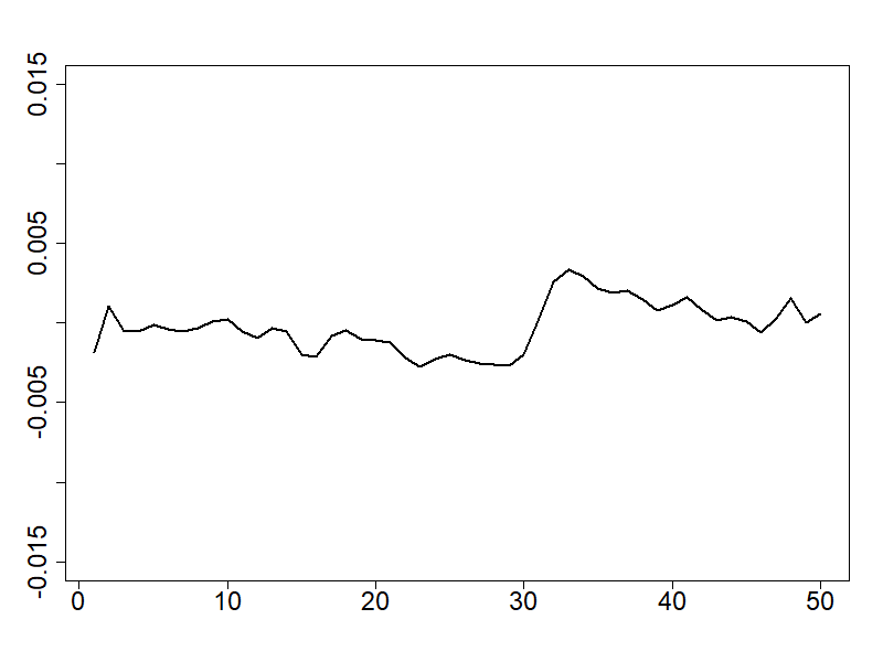
$\hat{\beta}^{(17)}$	$\hat{\beta}^{(18)}$	$\hat{\beta}^{(19)}$	$\hat{\beta}^{(20)}$
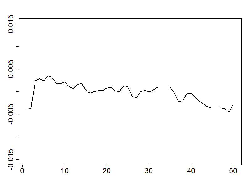
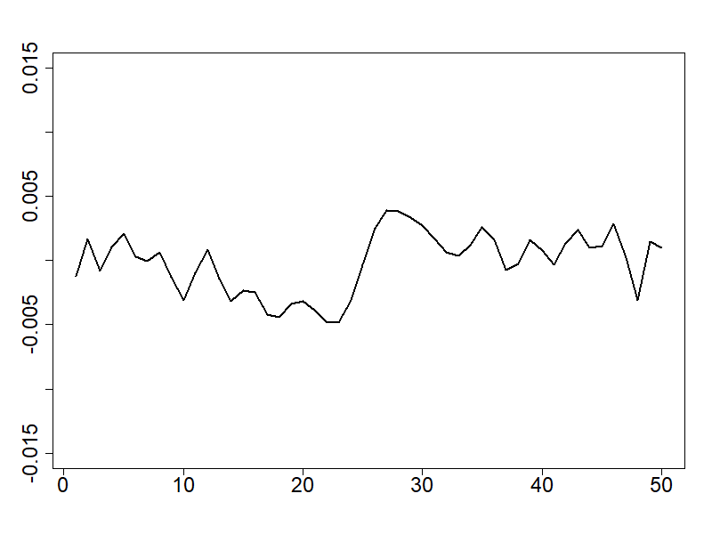
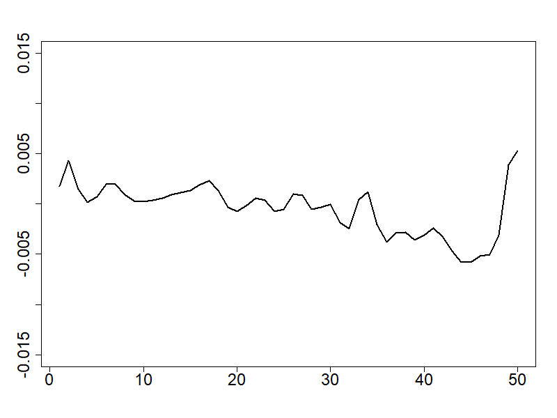
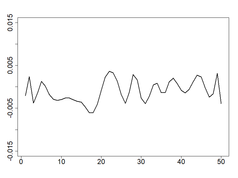
$\hat{\beta}^{(21)}$	$\hat{\beta}^{(22)}$	$\hat{\beta}^{(23)}$	$\hat{\beta}^{(24)}$
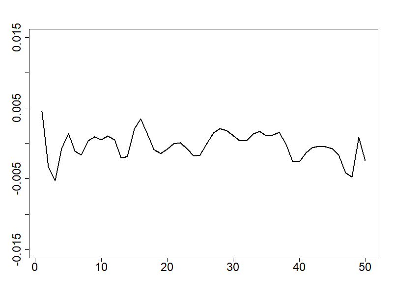
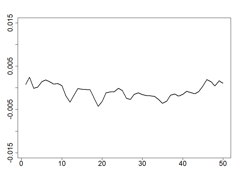
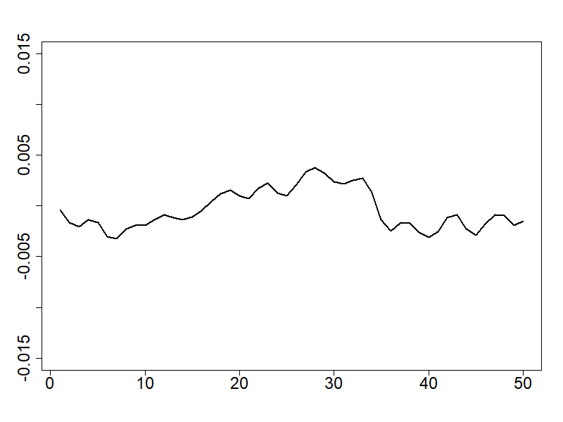
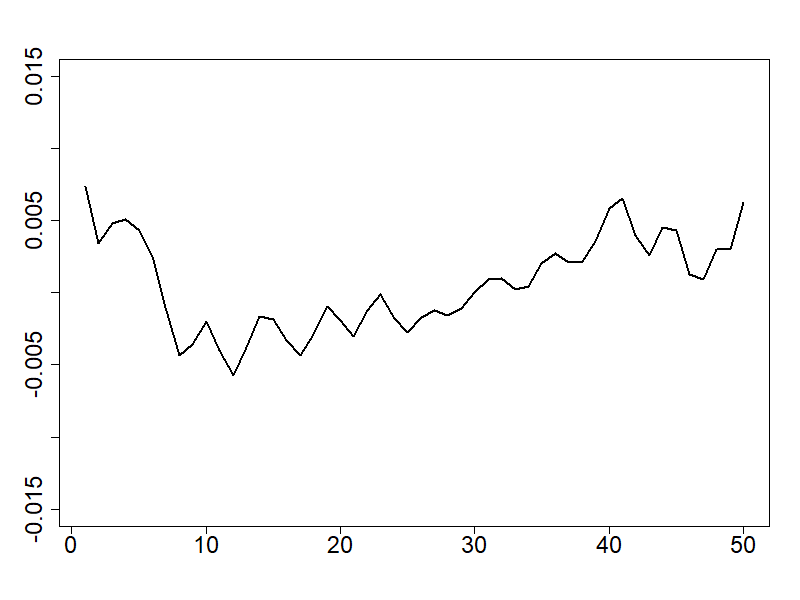
$\hat{\beta}^{(25)}$	$\hat{\beta}^{(26)}$	$\hat{\beta}^{(27)}$	$\hat{\beta}^{(28)}$

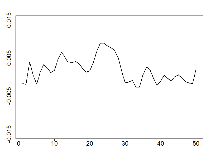
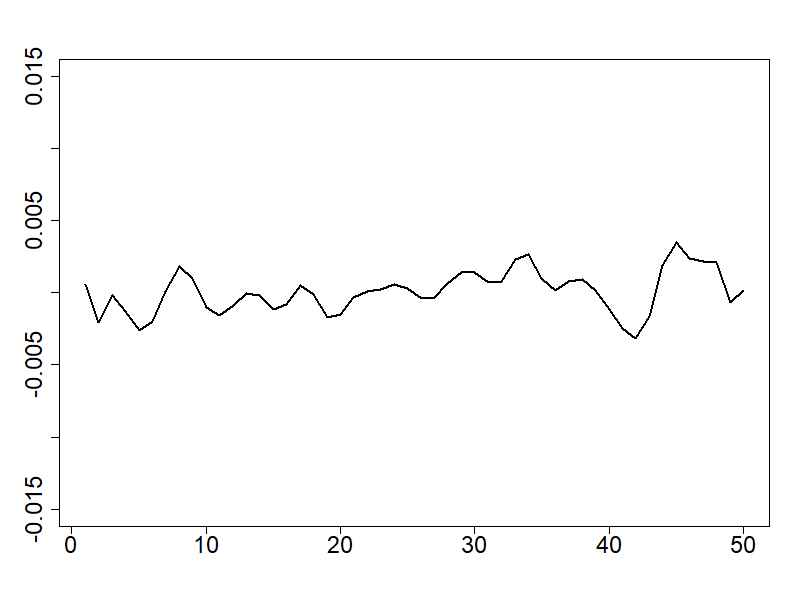
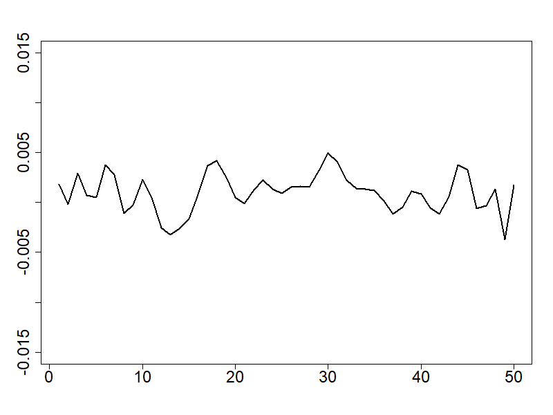
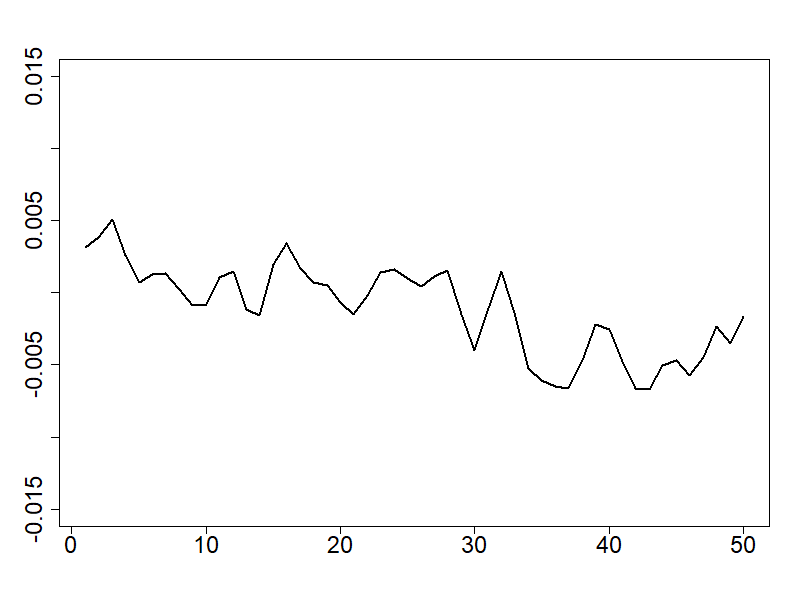
Figure 13: GL2 estimated coefficient model

Appendix B Proofs

Proof of Lemma 1.

Let the neighbor function $v$: $\{\mathscr{C}_{1},\mathscr{C}_{2},\ldots,\mathscr{C}_{p}\}\to\{1,2,\ldots,p\}$, as defined in Section 2.1 and $\mathscr{V}_{0}$, $\mathscr{V}_{1}$ defined as:

$$\mathscr{V}_{0}=\{i\in\{1,2,\ldots,p\},v^{2}(\mathscr{C}_{i})=i\}$$

and

$$\mathscr{V}_{1}=\{i\in\{1,2,\ldots,p\},i>v(\mathscr{C}_{i}),v^{2}(\mathscr{C}_{i})=i\},$$

with $v^{2}(\mathscr{C}_{i})$= $v(\mathscr{C}_{v(\mathscr{C}_{i})})$, for $i=1,\ldots,p$.
Observe that $i\in\mathscr{V}_{0}$ is equivalent to $v(\mathscr{C}_{i})\in\mathscr{V}_{0}$, and $i\in\mathscr{V}_{1}$ implies that $v(\mathscr{C}_{i})\not\in\mathscr{V}_{1}$. In other words, $\mathscr{V}_{0}$ is the set of indexes corresponding to conditions for which a $2$-cycle structure is present in the $1$-NN graph. $\mathscr{V}_{1}$ is a subset of $\mathscr{V}_{0}$ with $\text{card}\mathscr{V}_{1}=\frac{1}{2}\text{card}(\mathscr{V}_{0})$.
Then, for all $f\in\mathscr{H}$, we have

$$\sum_{j=1}^{p}||(\mathbf{L}f)^{(j)}||_{2} =\sum_{j\in\mathscr{V}_{0}}||f^{(j)}-f^{(v(\mathscr{C}_{j}))}||_{2}+\sum_{j\not\in\mathscr{V}_{0}}||f^{(j)}-f^{(v(\mathscr{C}_{j}))}||_{2}$$

$$=\sum_{j\in\mathscr{V}_{1}}||2(f^{(j)}-f^{(v(\mathscr{C}_{j}))})||_{2}+\sum_{j\not\in\mathscr{V}_{0}}||f^{(j)}-f^{(v(\mathscr{C}_{j}))}||_{2}.$$

Then, there exists a matrix $\mathbf{L}_{0}\in\mathbb{R}^{r\times p}$, with $r=p-\frac{1}{2}\text{card}(\mathscr{V}_{0})$, such as

$$\sum_{j=1}^{p}||(\mathbf{L}f)^{(j)}||_{2} =\sum_{j=1}^{r}||(\mathbf{L}_{0}f)^{(j)}||_{2}.$$

Since $v$ is constructed by the one-nearest neighbor graph–only 2-cycle structures can occur (Eppstein et al., , 1997)– then $\mathbf{L}_{0}$ is a full rank matrix. ∎

Proof of Proposition 1.

We borrow some reasoning from Tibshirani and Taylor, (2011) (the full-rank matrix case). In their paper, these authors were interested in the case where the penalty is defined using the $l1$ norm and a linear transformation of the coefficient in the multivariate case. We extend their reasoning to the $||\cdot||_{L_{2},1}$ norm and the setting of multivariate functional coefficients.

Notice that

$$||\mathbf{D}f||_{L_{2},1}=\sum_{j=1}^{r}||(\mathbf{L}_{0}f)^{(j)}||_{L_{2}}+\sum_{j=r+1}^{p}||(\mathbf{T}f)^{(j)}||_{L_{2}},\ \ f\in\mathscr{H}.$$

Using the definition of $\mathbf{L}_{0}$,

$$||\mathbf{D}f||_{L_{2},1}=||\mathbf{L}f||_{L_{2},1}+\sum_{j=r+1}^{p}||(\mathbf{T}f)^{(j)}||_{L_{2},1}.$$

Hence, the problem (3) can be written as

$$\hat{\beta}_{\lambda}=\operatorname*{arg\,min}_{f\in\mathscr{H}}\frac{1}{2}\sum_{i=1}^{n}\left(y_{i}-\langle x_{i},f\rangle_{\mathscr{H}}\right)^{2}+\sum_{j=1}^{p}\lambda\mathbb{I}(j\leq r)||(\mathbf{D}f)^{(j)}||_{L_{2}}$$ (19)

with $\mathbb{I}(\cdot)$ is the indicator function. The non-singularity of $\mathbf{D}$ implies

$$\hat{\psi}_{\lambda}=\operatorname*{arg\,min}_{f\in\mathscr{H}}\frac{1}{2}\sum_{i=1}^{n}\left(y_{i}-\langle x_{i},\mathbf{D}^{-1}f\rangle_{\mathscr{H}}\right)^{2}+\sum_{j=1}^{p}\lambda\mathbb{I}(j\leq r)||f^{(j)}||_{L_{2}},$$ (20)

with $\hat{\psi}_{\lambda}=\mathbf{D}\hat{\beta}_{\lambda}$. The equality $\langle(\mathbf{D}^{-1})^{\operatorname*{\top}}x_{i},f\rangle_{\mathscr{H}}=\langle x_{i},\mathbf{D}^{-1}f\rangle_{\mathscr{H}}$ concludes the proof. ∎

Proof of Lemma 2.

To simplify the notation, let denote by $f_{\mathscr{I}_{k}}$ the function composed only of the set of dimensions of $f\in\mathscr{H}$ which belong to $\mathscr{I}_{k}$.

The proof of the lemma relies on the following statements:

1. For $f\in\mathscr{H}$,

   $$||f_{\mathscr{I}_{p_{k}}}-\bar{f}_{\mathscr{I}_{k}}\vec{1}_{p_{k}}||_{L_{2},2}=||\mathrm{R}_{k}f_{\mathscr{I}_{k}}||_{L_{2},2}.$$

   for all $k\in\{1,\ldots,K\}$.

2. The matrices $\bar{\mathbf{M}}$ and $\mathbf{R}$ are such that $\mathbf{R}\bar{\mathbf{M}}^{\top}=\mathbf{0}_{(p-K)\times K}$

For the first point (a), direct calculation shows that

$$f_{\mathscr{I}_{k}}-\bar{f}_{\mathscr{I}_{k}}\vec{1}_{p_{k}} =\underbrace{\left[\mathbb{I}_{p_{k}\times p_{k}}-\displaystyle\frac{1}{p_{k}}\mathbf{1}_{p_{k}\times p_{k}}\right]}_{\mathrm{P}_{k}}f_{\mathscr{I}_{k}}.$$ (21)

The rank of $\mathrm{P}_{k}$ is $p_{k}-1$. Let $\mathrm{R}_{k}$ be the R reduced rank matrix of size $(p_{k}-1)\times|p_{k}|$ obtained by the QR decomposition of $\mathrm{P}_{k}$. Since $||\cdot||_{L_{2},2}$ is the Frobenius function norm, we have (a), i.e. $||\mathrm{P}_{k}f_{\mathscr{I}_{k}}||_{L_{2},2}=||\mathrm{R}_{k}f_{\mathscr{I}_{k}}||_{L_{2},2}$.
For point (b), without loss of generality, we assume that

$$\mathbf{M}=\begin{pmatrix}\vec{1}_{p_{1}}^{\operatorname*{\top}}&\vec{0}_{p_{2}}^{\operatorname*{\top}}&...&0\\ \vec{0}_{p_{1}}^{\operatorname*{\top}}&\vec{1}_{p_{2}}^{\operatorname*{\top}}&...&0\\ ...&&&...\\ \vec{0}_{p_{1}}^{\operatorname*{\top}}&\vec{0}_{p_{2}}^{\operatorname*{\top}}&...&\vec{1}_{p_{K}}^{\operatorname*{\top}}\end{pmatrix}.$$

Note that $\vec{1}_{p_{k}}$ belongs to the kernel of $\mathrm{P}_{k}$, i.e $\mathrm{P}_{k}\vec{1}_{p_{k}}=\vec{0}_{p_{k}}$, for all $k\in\{1,\ldots,K\}$. From the definition of $\mathrm{R}_{k}$,it follows that $\mathrm{P}_{k}=\mathrm{Q}_{k}\begin{pmatrix}\mathrm{R}_{k}\\ \mathbf{0}_{p_{k}}^{\operatorname*{\top}}\end{pmatrix}$, where $\mathrm{Q}_{k}$ is an orthogonal matrix. Then, $\mathrm{P}_{k}\vec{1}_{k}=\mathbf{0}_{p_{k}}$ implies that $\mathrm{R}_{k}\vec{1}_{k}=\mathbf{0}_{p_{k}-1}$. As $\mathrm{R}_{k}\vec{1}_{k}=\mathbf{0}_{p_{k}-1}$ for all $k\in\{1,\ldots,K\}$, we have

$$\mathbf{R}\bar{\mathbf{M}}^{\top}=\mathbf{0}_{(p-K)\times K}.$$

Finally, as a direct consequence of (a), the matrix $\mathbf{G}_{\alpha}$ satisfies the relation (11). Observe that $\mathbf{G}_{\alpha}$ is non-singular as a consequence of (b). This concludes the proof. ∎

Proof of Proposition 3.

• The equation (14) implies that for each dimension $j$, $j=1,\ldots,p$, we have

  $$\beta^{(j)}(t) =(b^{(j)})^{\operatorname*{\top}}\phi(t),$$

  where $b^{(j)}\in\mathbb{R}^{M}$ $\;t\in[0,T]$.
  Define $\mathrm{F}$= $\{\langle\phi_{i},\phi_{j}\rangle\}_{i,j}$ and $\mathrm{F}=(\mathrm{F}^{1/2})^{\operatorname*{\top}}\mathrm{F}^{1/2}$. Thus, we have

  $$||\beta^{(j)}||_{L_{2}}=||(\mathrm{F}^{1/2})^{\operatorname*{\top}}b^{(j)}||_{2}=||(b^{(j)})^{\operatorname*{\top}}\mathrm{F}^{1/2}||_{2}.$$

  Moreover,

  $$\mathbf{B}\text{F}^{1/2}=\begin{pmatrix}(b^{(1)})^{\operatorname*{\top}}\\ (b^{(2)})^{\operatorname*{\top}}\\ ...\\ (b^{(p)})^{\operatorname*{\top}}\end{pmatrix}\text{F}^{1/2}=\begin{pmatrix}(b^{(1)})^{\operatorname*{\top}}\text{F}^{1/2}\\ (b^{(2)})^{\operatorname*{\top}}\text{F}^{1/2}\\ ...\\ (b^{(p)})^{\operatorname*{\top}}\text{F}^{1/2}\end{pmatrix},$$

  and $||\beta||_{L_{2},1}=||\mathbf{B}\mathrm{F}^{1/2}||_{2,1}$.

• Notice that $a_{i}=\text{vec}(\mathbf{A}_{i}^{\operatorname*{\top}})$, $b=\text{vec}(\mathbf{B}^{\operatorname*{\top}})$ with vec($\cdot$) denotes the vectorization operator. It follows that

  $$b_{0} =\text{vec}((\mathbf{Z}\mathbf{B})^{\operatorname*{\top}})=\text{vec}(\mathbf{B}^{\operatorname*{\top}}\mathbf{Z}^{\operatorname*{\top}})$$

  $$=(\mathbf{Z}\otimes\mathrm{I}_{M\times M})\text{vec}(\mathbf{B}^{\operatorname*{\top}})=(\mathbf{Z}\otimes\mathrm{I}_{M\times M})b,$$

  with $\otimes$ denotes the Kronecker Product.

∎

References

- Aguilera et al., (2006) Aguilera, A. M., Escabias, M., and Valderrama, M. J. (2006). Using principal components for estimating logistic regression with high-dimensional multicollinear data. Computational Statistics & Data Analysis, 50(8):1905–1924.
- Beyaztas and Lin Shang, (2022) Beyaztas, U. and Lin Shang, H. (2022). A robust functional partial least squares for scalar-on-multiple-function regression. Journal of Chemometrics, 36(4):e3394.
- Bleakley and Vert, (2011) Bleakley, K. and Vert, J.-P. (2011). The group fused lasso for multiple change-point detection. arXiv preprint arXiv:1106.4199.
- Cardot et al., (1999) Cardot, H., Ferraty, F., and Sarda, P. (1999). Functional linear model. Statistics & Probability Letters, 45(1):11–22.
- Chen and Müller, (2012) Chen, K. and Müller, H.-G. (2012). Modeling repeated functional observations. Journal of the American Statistical Association, 107(500):1599–1609.
- Eppstein et al., (1997) Eppstein, D., Paterson, M. S., and Yao, F. F. (1997). On nearest-neighbor graphs. Discrete & Computational Geometry, 17(3):263–282.
- Escabias et al., (2005) Escabias, M., Aguilera, A., and Valderrama, M. (2005). Modeling environmental data by functional principal component logistic regression. Environmetrics: The official journal of the International Environmetrics Society, 16(1):95–107.
- Godwin, (2013) Godwin, J. (2013). Group lasso for functional logistic regression. Master’s thesis.
- Górecki et al., (2015) Górecki, T., Krzyśko, M., and Wołyński, W. (2015). Classification problems based on regression models for multi-dimensional functional data. Statistics in Transition new series, 16(1).
- Ismail Fawaz et al., (2020) Ismail Fawaz, H., Lucas, B., Forestier, G., Pelletier, C., Schmidt, D. F., Weber, J., Webb, G. I., Idoumghar, L., Muller, P.-A., and Petitjean, F. (2020). Inceptiontime: Finding alexnet for time series classification. Data Mining and Knowledge Discovery, 34(6):1936–1962.
- Jacob et al., (2009) Jacob, L., Obozinski, G., and Vert, J.-P. (2009). Group lasso with overlap and graph lasso. In Proceedings of the 26th annual international conference on machine learning, pages 433–440.
- Jacques and Preda, (2014) Jacques, J. and Preda, C. (2014). Model-based clustering for multivariate functional data. Computational Statistics & Data Analysis, 71:92–106.
- Land and Friedman, (1997) Land, S. R. and Friedman, J. H. (1997). Variable fusion: A new adaptive signal regression method.
- Lukas and Meier, (2020) Lukas and Meier (2020). Package ‘grplasso’.
- Meier et al., (2008) Meier, L., Van De Geer, S., and Bühlmann, P. (2008). The group lasso for logistic regression. Journal of the Royal Statistical Society: Series B (Statistical Methodology), 70(1):53–71.
- Moindjié et al., (2022) Moindjié, I.-A., Dabo-Niang, S., and Preda, C. (2022). Classification of multivariate functional data on different domains with partial least squares approaches. arXiv preprint arXiv:2212.09145.
- Preda and Saporta, (2002) Preda, C. and Saporta, G. (2002). Régression pls sur un processus stochastique. Revue de statistique appliquée, 50(2):27–45.
- Ramsey and Silverman, (2005) Ramsey, J. O. and Silverman, B. W. (2005). Functional Data Analysis. Springer-Verlag, 2 edition.
- Ruiz et al., (2021) Ruiz, A. P., Flynn, M., Large, J., Middlehurst, M., and Bagnall, A. (2021). The great multivariate time series classification bake off: a review and experimental evaluation of recent algorithmic advances. Data Mining and Knowledge Discovery, 35(2):401–449.
- Tibshirani et al., (2005) Tibshirani, R., Saunders, M., Rosset, S., Zhu, J., and Knight, K. (2005). Sparsity and smoothness via the fused lasso. Journal of the Royal Statistical Society: Series B (Statistical Methodology), 67(1):91–108.
- Tibshirani and Taylor, (2011) Tibshirani, R. J. and Taylor, J. (2011). The solution path of the generalized lasso. The annals of statistics, 39(3):1335–1371.
- Yi et al., (2022) Yi, Y., Billor, N., Liang, M., Cao, X., Ekstrom, A., and Zheng, J. (2022). Classification of eeg signals: an interpretable approach using functional data analysis. Journal of Neuroscience Methods, 376:109609.
- Yuan et al., (2011) Yuan, L., Liu, J., and Ye, J. (2011). Efficient methods for overlapping group lasso. Advances in neural information processing systems, 24.
- Yuan and Lin, (2006) Yuan, M. and Lin, Y. (2006). Model selection and estimation in regression with grouped variables. Journal of the Royal Statistical Society: Series B (Statistical Methodology), 68(1):49–67.
- Zou and Hastie, (2005) Zou, H. and Hastie, T. (2005). Regularization and variable selection via the elastic net. Journal of the Royal Statistical Society Series B: Statistical Methodology, 67(2):301–320.