Reducing the number of qubits by a half in one dimensional quantum simulations of Ising chains

Abstract

We investigate the Ising model using the Block Renormalization Group Method (BRGM), focusing on its behavior across different system sizes. The BRGM reduces the number of spins by a factor of 1/2, effectively preserving essential physical features of the Ising model while using only half the spins. Through a comparative analysis, we demonstrate that as the system size increases, there is a convergence between results obtained from the original and renormalized Hamiltonians, provided the coupling constants are redefined accordingly. Remarkably, for a spin chain with 24 spins, all physical features, including magnetization, correlation function, and entanglement entropy, exhibit an exact correspondence with the results from the original Hamiltonian. The success of BRGM in accurately characterizing the Ising model, even with a relatively small number of spins, underscores its robustness and utility in studying complex physical systems, and facilitates its simulation on current NISQ computers, where the available number of qubits is largely constrained.

1 Introduction

The Ising model holds a prominent position in the history of physics and the development of various physics fields, including condensed matter physics and statistical mechanics. Being simply an arrangement of spin variables, with two possible values (representing molecules, particles, neurons, etc), and subjected to nearest-neighbor interactions with an additional local external field, it amazingly finds applications in a wealth of natural (from biological neural networks to ecology or the spread of diseases), artificial (e.g. artificial intelligence) and social systems (e.g. voters model). Its simpler version in one dimension was solved initially by Ernst Ising, after the proposal of his supervisor, Wilhem Lenz, to solve it in higher dimensions, not knowing that the complexity it beared had to wait for many years of advancement of science to be solved [1, 2]. Our interest in the Ising model in one dimension here is substantiated by its capability to encode mathematical and computational problems. There is a famous correspondence of Ising models with quadratic unconstrained binary optimization problem (QUBO) with boolean variables. This lies the connection of finding the ground state of the Ising model to optimization problems, and therefore to solution of problems such as the first proposed Boolean satisfiability problem [3, 4]. Indeed the connection with satisfiability problems allowed to establish that finding the ground state is a NP-hard problem for two and three dimensions [5].

The growth of the number of possible configurations as $2^{N}$, for $N$ spins is ultimately behind this complexity, and this points to a clear connection: what if spin variables are modelled as quantum two-state variables, i.e. qubits, and one allows the problem to perform a quantum evolution towards its ground state? this is the underlying idea with the utilization of quantum systems to simulate spin Ising models [6]. This connection led to two strategies: to develope approximate methods, often quantum inspired, to solve the problem; and to use directly a quantum computer.

The first strategy derived in a list of techniques, such as the Density Matrix Renormalization Group (DMRG) [7, 8], Matrix Product States, and related methods (see, for example [9],[10]). One can also make use of methods which are based on the Lie-Trotter formula [11], Krylov subspace expansion [12], truncated Taylor series [13] or randomized product formulae [14, 15, 16]. This collection of techniques allowed to obtain results fruitful also for the very development of physics. We address the reader to [17] for a recent review regarding a comparative performance of these methods.

The second strategy required the development and reliable functioning at sufficiently large sizes of quantum computers. One option is to mimic the well known Monte Carlo-based method of simulated annealing, termed as quantum annealing. This has been implemented even in commercial set-ups for thousands of qubits [18, 19]. Also, one can use quantum gate-based computers and implement various algorithms, see e.g. [20]. Most of the above approximate methods can also be used for this purpose, or in combination with hybrid optimisation methods [21, 14].

This second strategy, which evidently can lead to the most efficient methods, finds its limitation in the number of practical qubits available. For quantum annealing methods, current technology allows for the order of a few thousands while for quantum gate systems it is at present limited to a few hundreds (see e.g. [22]). But the practical problems e.g. boolean satisfiability, require even millions of variables [23].

In this technological context, reducing the number of qubits is crucial for being able to simulate larger many-body systems on current available NISQ (Noisy Intermediate-Scale Quantum) processors. In this paper we introduce and test a tool which can be used to reduce the number of qubits needed to solve a particular problem by one half. To this end we employ a well-established theoretical framework known as Renormalization Group theory (RG), which has been developed over the course of many years. The RG theory involves a series of systematic steps that aim to reduce the number of spins in the system while simultaneously redefining the original couplings between them. These steps are iterated multiple times, leading to a progressive reduction in the number of spins. By employing this iterative process, researchers are able to extract valuable information regarding the critical behavior of the system, contributing to our understanding of its fundamental properties [24, 25, 26, 27].

In particular, we concentrate on the Block RG Method (BRGM), which makes use of the concept of blocks already introduced by Kadanoff [25, 28, 29, 30]. This method shares some similarities with the DMRG method. In both cases, one makes a choice of such blocks and performs some truncation on the eigenstates. However, while in the latter approach one chooses the eigenstates of the corresponding density matrix matrix with the highest eigenvalues, for the BRGM one keeps the lowest energy states of the block Hamiltonian, i.e. we perform the RG procedure in “real space”. As it has been shown, a wise choice of these blocks and, in particular of the distribution of spin couplings inside and among the blocks (the so-called “intrablock” and “interblock” terms, respectively) can provide a good approximation to the study of critical phenomena in these systems [30, 31, 32, 33].

The focus of our investigation implies a new approach, as it revolves around determining whether the BRGM iteration process yields meaningful results within a finite number of steps. To address this, we have conducted a thorough examination of the BRGM applied to the Ising model, utilizing a comparative analysis of relevant quantities. Our methodology involved systematically reducing the number of spins by a factor of 1/2 while appropriately adjusting the coupling constants. Remarkably, even with a relatively small number of spins, we have observed an excellent agreement between the obtained results and the ones that correspond to the original, larger Hamiltonian. These findings highlight the efficacy of the BRGM iteration procedure in accurately characterizing the relevant properties of the Ising model, supporting its utility as a valuable tool in the study of complex physical systems using an effectively reduced number of spins.

The structure of this paper is organized as follows: Sec.Sec. 2 offers a brief overview of the theoretical foundations of the BRGM. We delve into the key concepts and principles underlying this approach, providing a concise review of the theory and its application in the context of the Ising model. Building upon this theoretical foundation, Sec. 3 focuses on our investigation of the physical features of the Ising model using the BRGM approach. We introduce the magnetization, correlation functions, and entanglement entropy of the system for various number of spins. Section 4 is dedicated to the presentation and discussion of our findings. We compare and contrast the results for different spin numbers, and discuss their implications. Finally, in Sec. 5 we provide a comprehensive conclusion based on our results, and discuss the broader implications of our study.

2 A Brief Review of the BRGM

The method we follow here is based on a block spin transformation that preserves the structure of the model [32]. We start from the Ising Hamiltonian subject to an external magnetic field, defined as

$$H=-\sum_{i=1}^{N}J_{i}\sigma_{i}^{z}\sigma_{i+1}^{z}-\sum_{i=1}^{N}\Gamma_{i}\sigma_{i}^{x},$$ (1)

where $\sigma_{i}^{z}$ and $\sigma_{i}^{x}$ are Pauli matrices acting on the $i$th spin, and $N$ is assumed to be even. We assume periodic boundary conditions. Then we divide the chain into blocks of two spins. We assume this Hamiotonian encodes in the coefficients $J_{i}$ and $\Gamma_{i}$ some practical problem one aims to solve.

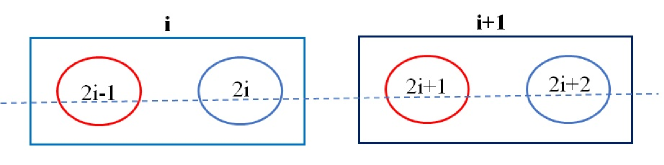
Fig. 1: Generation of block spin formations in a one-dimensional setting.

The initial Hamiltonian is split into intrablock and interblock parts [34] (see Figure. 1) giving rise to

$$H_{i}^{\rm{intra}}=-J_{2i-1}\sigma_{2i-1}^{z}\sigma_{2i}^{z}-\Gamma_{2i-1}\sigma_{2i-1}^{x},$$ (2)

$$H_{i,i+1}^{\rm{inter}}=-J_{2i}\sigma_{2i}^{z}\sigma_{2i+1}^{z}-\Gamma_{2i}\sigma_{2i}^{x},$$ (3)

where spins $2i\!-\!1$ and $2i$ belong to block $i$, and spin $2i\!+\!1$ belongs to block $i\!+\!1$. The label $i$ of block then runs from 1 to N/2. Now, we compute the eigenvalues of $H_{i}^{\rm{intra}}$ as follows

$$\varepsilon_{i}^{(1)}=\varepsilon_{i}^{(2)}=-\sqrt{(J_{2i-1})^{2}+(\Gamma_{2i-1})^{2}},$$ (4a)

$$\varepsilon_{i}^{(3)}=\varepsilon_{i}^{(4)}=\sqrt{(J_{2i-1})^{2}+(\Gamma_{2i-1})^{2}}.$$ (4b)

As we see, these are degenerate. The corresponding eigenvectors are

$$\ket{1}_{i}=a_{i}^{+}\ket{\uparrow\uparrow}+a_{i}^{-}\ket{\downarrow\uparrow},$$ (5a)

$$\ket{2}_{i}=a_{i}^{+}\ket{\downarrow\downarrow}+a_{i}^{-}\ket{\uparrow\downarrow},$$ (5b)

$$\ket{3}_{i}=a_{i}^{-}\ket{\downarrow\downarrow}-a_{i}^{+}\ket{\uparrow\downarrow},$$ (5c)

$$\ket{4}_{i}=a_{i}^{-}\ket{\uparrow\uparrow}-a_{i}^{+}\ket{\downarrow\uparrow},$$ (5d)

where

$$a_{i}^{\pm}=\sqrt{\frac{1}{2}(1\pm\frac{J_{2i-1}}{(J_{2i-1})^{2}+(\Gamma_{2i-1})^{2}})},$$ (6)

and $\ket{\uparrow\uparrow},\ket{\downarrow\uparrow},\ket{\uparrow\downarrow},\ket{\downarrow\downarrow}$ is the orthonormal basis in the $\sigma_{z}$ basis, i.e, $\sigma_{z}\ket{\uparrow}=\ket{\uparrow},$ $\sigma_{z}\ket{\downarrow}=-\ket{\downarrow}$. We keep the two lowest-lying energy eigenstates $\ket{1}_{i}$ and $\ket{2}_{i}$, and drop the others. We then replace each block with a single spin represented by the $\ket{1}_{i}$ and $\ket{2}_{i}$ states. To this end, we define the projector onto the coarse-grained system as

$$P=\bigotimes_{i=1}^{N/2}P_{i},$$ (7)

where $P_{i}$ is the projector

$$P_{i}=(\ket{1}\bra{1}+\ket{2}\bra{2})_{i}.$$ (8)

The resulting coarse-grained Hamiltonian $H_{\rm{RG}}$ is defined by the projection

$$H_{\rm{RG}}=PHP=\sum_{i=1}^{N/2}\varepsilon_{i}^{(1)}1_{i}-\sum_{i=1}^{N/2}\tilde{J_{i}}\tilde{\sigma_{i}^{z}}\tilde{\sigma_{i+1}^{z}}-\sum_{i=1}^{N/2}\tilde{\Gamma_{i}}\tilde{\sigma_{i}^{x}},$$ (9)

where re-normalized couplings are

$$\tilde{J_{i}}=\frac{J_{2i}J_{2i+1}}{\sqrt{(J_{2i+1})^{2}+(\Gamma_{2i+1})^{2}}},$$ (10a)

$$\tilde{\Gamma_{i}}=\frac{\Gamma_{2i-1}\Gamma_{2i}}{\sqrt{(J_{2i-1})^{2}+(\Gamma_{2i-1})^{2}}}.$$ (10b)

As we can see, this transformation preserves the form of the initial Hamiltonian defined in Eq. (1) except for the first term in Eq. (9), which is proportional to the identity [32] and can be neglected.

3 Investigation of Physical Features of Ising Model with the Use of the BRGM

In what follows, we will investigate the application of the BRGM approach to an Ising spin chain system with different sizes, i.e. to different values of $N$. Our aim is to apply the renormalization procedure to each chain, which implies a reduction in the number of spins by a factor $1/2$. We will examine key observables, including magnetization, correlation functions, and entanglement entropy, that will be compared to calculations obtained with the original Hamiltonian. We will progressively increase the number of initial spins, by considering the cases with $N=6$, $N=12$, and $N=24$. From this study, we will show that already for $N=24$ the original and the renormalized Hamiltonians produce the same outputs. This analysis will contribute to our understanding of the BRGM method’s efficacy in capturing relevant features and provide valuable insights into the properties of reduced spin chain systems.

3.1 Magnetization

Magnetization is a property of magnetic materials that describes the degree of alignment of its spins. In the context of the Ising chain Hamiltonian, which was firstly introduced as a mathematical model used to study magnetic systems, magnetization is the total magnetic moment of the system, which is the sum of the magnetic moments of each individual spin. The Ising chain Hamiltonian is computed by summing up the interactions between neighboring spins, which are either ferromagnetic or antiferromagnetic depending on the sign of the interaction strength [35, 36, 37]. To compute the magnetization of the Ising chain, one computes the expected value of the individual spins on the present state, and performs a sum over them. This allows one to study the behavior of the magnetization as a function of other physical parameters, and to investigate possible phase transitions that occur in magnetic systems. The formula to compute the magnetization for the considered system with $N$ spins is therefore [38]

$$M(t)=\frac{1}{N}\sum_{i=1}^{N}\bra{\Psi(t)}\sigma_{z}^{i}\ket{\Psi(t)},$$ (11)

where $M(t)$ is the magnetization at time $t$, $\ket{\Psi(t)}$ denotes the quantum state of the system at that time, and the summation is taken over all $N$ spins in the system. The magnetization can be positive, negative, or zero depending on the orientation of the individual magnetic moments and the strength of the interactions between them.

3.2 Spin Correlation Functions

A spin correlation function is a quantity that characterizes the degree of correlation between the spins at different positions. In the context of spin model like the present one, the spin correlation function is typically defined as the difference between averaging the product of the spin values separated by a distance $r$, and the product of the average spin values, where“average” means expected value [39, 40, 41, 42]. The spin correlation function for our considered model is given by

$$C^{i}(r)=\langle\sigma_{z}^{i}\sigma_{z}^{i+r}\rangle-\langle\sigma_{z}^{i}\rangle\langle\sigma_{z}^{i+r}\rangle,$$ (12)

where we are comparing spins at $i$ and $i\!+\!r$ positions.

In our study, we focus on analyzing the spin correlation function within the framework of our considered Ising model. Through comprehensive investigations and numerical simulations, we aim to elucidate the effects of renormalization procedures on the spin correlation function and assess the extent to which the renormalization group method preserves the characteristic correlation properties of the model.

3.3 Entanglement Entropy

Entanglement entropy is a quantity that characterizes the amount of quantum entanglement between two parts of a larger quantum system. The entanglement entropy is computed by dividing the system into two parts, $A$ and $B$, and then tracing out the degrees of freedom in region $B$ to obtain the reduced density matrix for region $A$ [43, 44]. In this work, the entanglement entropy $S$ is computed as the Von Neumann entropy of this reduced density matrix, as follows

$$S=-\rm{Tr}(\rho_{A}log(\rho_{A})),$$ (13)

where $\rho_{A}$ is the reduced density matrix for region $A$, obtained by tracing out the degrees of freedom in region $B$, and $\rm{Tr}$ denotes the trace over the Hilbert space of region $A$. In our analysis of the transverse Ising model, we consider two regions, $A$ and $B$, with $x=1$ spins in region $A$ and $N-x=N-1$ spins in region $B$. It is worth noting that, for the special case when $x=N/2$, the result is the same. In this scenario, the entanglement entropy still exhibits a logarithmic scaling with the size of the boundary between regions $A$ and $B$, indicating the presence of long-range entanglement in the system. The entanglement entropy can be used to study the behavior of the system as a function of the magnetic field strength, and to identify phase transitions and critical points in the system  [45].

4 Results and Discussion

We have developed a code with Qutip where each spin is a qubit and we perform the quantum evolution of the reduced RG Hamiltonian $H_{\rm{RG}}$ and the initial one, to compare among them. To perform such calculations we made use of the Lluis Vives computer from University of Valencia, Spain. Lluis Vives is an Altix UltraViolet 1000 server from the Silicon Graphics company. It has 64 Xeon 7500 series hexacore CPUs at 2.67 GHz and 18 MB of on-die L3 cache, 2048 GB of RAM and about 15 TB of hard disk. We have calculated with an increasing even number of spins, finding good results for $N=24$ spins, which is also already close to the limit we found of the computational capability. These are proof-of-concept calculations. With these results, we show that one can implement the reduced Hamiltonian in a real quantum computer and perform the evolution on the physical system to simulate with the RG Hamiltonian $H_{\rm{RG}}$ given in Eq. (9). The results obtained will then be helpful to solve the practical problem which may be encoded in the coefficients of the corresponding Hamiltonian of interest Eq. (1).

In the following figures, we depict four different scenarios for each of the magnitudes defined in the previous Section, as one increases the number $N$ of spins. We show results for four cases: For the original Hamiltonian $H$ (Eq. (1)); The same original Hamiltonian with half of the initial number of spins and the initial couplings; The renormalized Hamiltonian ($H_{\rm{RG}}$) with original coefficients; And for the RG Hamiltonian ($H_{\rm{RG}}$) with modified coefficients given in Eqs. 10a and 10b. The purpose of this comparison is to assess the importance of performing the RG in a consistent way, i.e. by a proper redefinition of the couplings. For the initial comparisons, we consider an homogeneous Ising model, for which all $J_{i}$ take the same value (indicated by $J$), and similarly for $\Gamma_{i}$, which will be denoted as $\Gamma$. At the end of this section we also analyze a more general situation, which involves assigning random values of the couplings at each site, to check the validity of our results.

Figure 2 shows these results for the magnetization for different numbers of spins. Figure 2 (a) corresponds to $N=6$ spins, Figure 2 (b) to $N=12$ and Figure 2 (c) to $N=24$ spins. Upon analyzing the figures representing the magnetization of the original Hamiltonian of the Ising model and its corresponding renormalized Hamiltonian as $N$ is increased, one observes a clear convergence between both of them, while the two remaining curves show a different behavior. Indeed, for the case of 24 spins, Figure 2 (c), the magnetization curves for both systems exhibit a remarkable coincidence. As we will see later, this convergence is confirmed by computing different observables.

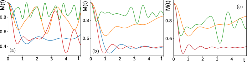
Fig. 2: Total magnetization as a function of time. Panels (a), (b), and (c) corrspond to $N=6,12$ and 24 spin respectively. In every panel blue curve corresponds to the original Hamiltonain; Orange curve is the result for the original Hamiltonian with half of the initial number of spins and the initial couplings; Green curve corresponds to the renormalized Hamiltonian ($H_{\rm{RG}}$) with original coefficients; Finally red curve is the result for the RG Hamiltonian ($H_{\rm{RG}}$) with modified coefficients. The original coefficients are taken as $J=1$ and $\Gamma=1/2$. All magnitudes are adimensional.

Figure 3 presents a comprehensive analysis of the correlation function as defined by Eq. 12 for $i=1$ and $r=1$ (we also explore there is again a clear convergence from the results derived from the BRGM Hamiltonian, with one half the original spins, towards the initial Hamiltonian, provided the renormalized coupling constants are adopted, at variance with other strategies. The degree of achieved coincidence for $N=24$ spins is striking. Conversely, any other choice (green and orange curves) gives very different results.

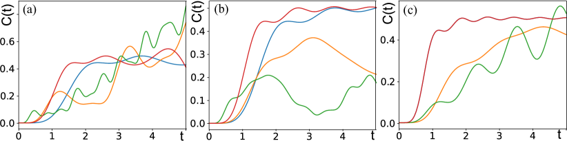
Fig. 3: The spin correlation function for $i=1$ and $r=1$ as a function of time for (a) $N=6$ spins, (b) $N=12$ spins, (c) $N=24$ spins. The correlation function given in Eq. 12 is compared in the same four instances as in Figure 2 (same color code). The original coefficients are taken as $J=1$ and $\Gamma=1/2$. All magnitudes are adimensional.

Figure 4 provides an in-depth examination of the entanglement entropy through the depiction of the same four distinct scenarios depicted in the previous two figures. The same comments hold in this case. A complete agreement is found for the case with $24$ spins.

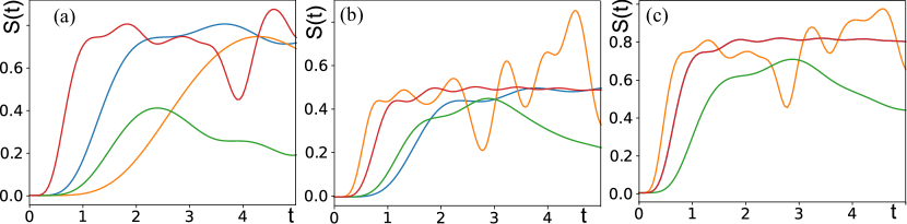
Fig. 4: The entanglement entropy as a function of time for (a) $N=6$ spins, (b) $N=12$ spins, (c) $N=24$ spins. The entanglement entropy given in Eq. (13) is compared in the same four instances as in Figure 2 (same color code). The original coefficients are taken as $J=1$ and $\Gamma=1/2$. All magnitudes are adimensional.

To conclude, we calculate for an initial Hamiltonian with random coefficients, particularly ($J_{i}$ and $\Gamma_{i}$ randomly chosen in the range of 0 and 1). We find the same results as in previous cases. We show directly the results for all three magnitudes and for $N=24$ in Figure 5. There is again a great overlap between the physical features of the original Hamiltonian and the renormalized Hamiltonian. This research contributes to the existing knowledge by highlighting the significance of this overlap in the general case. We find that regardless of the values for coefficients, the resulting outcome for physical features of a system contains 24 spins under BRGM is identical.

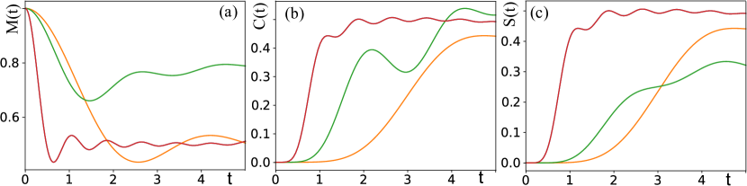
Fig. 5: (a) Magnetization, (b) Spin correlation function, (c) The entanglement entropy as a function of time for 24 spins. We present the results for the same four instances as in Figure 2 (same color code). The original coefficients $J_{i}$ and $\Gamma_{i}$ where obtained as random numbers within the interval [0,1]. All magnitudes are adimensional.

5 Conclusions

In conclusion, our analysis of the Ising model using the Block Renormalization Group Method (BRGM) has yielded valuable insights into the behavior of physical features such as magnetization, correlation function and entanglement entropy across different system sizes. The method implies a change in the number of spins by a factor $1/2$, which is a dramatic reduction in practical terms, since the dimension of the associated Hilbert space scales as $2^{N}$. We compared the results obtained from the original Hamiltonian with those from the renormalized one, and we observed that, as the value of $N$ is increased, there is a clear convergence between both Hamiltonians, provided that the coupling constants are redefined accordingly, within the spirit of the BRGM. In fact, for spin chains comprising 24 spins, all these features exhibited an exact correspondence with the results obtained with the original Hamiltonian. This remarkable similarity suggests that the BRGM successfully preserves, already at this size, the essential physical characteristics of the Ising model while making use of just half the spins. We emphasize that the technique fails for small systems, so it is necessary that a sufficiently large problem is tackled when using this tool.

Although our calculations were performed on a classical computer, the techniques involved in the BGRM can be easily exported to a quantum computer, allowing to obtain exact results with one half the qubits needed to simulate the original Hamiltonian. Reducing the amount of required resources is of fundamental importance in the NISQ era, where quantum processors are severely constrained by their limited number of qubits.

The computation for the spin chain with 24 spins presented a significant computational challenge. To overcome this hurdle, we utilized the computational resources of the Lluis Vives machine at the Valencia University in Spain. The availability of such a powerful computing platform enabled us to accurately perform the necessary calculations and obtain reliable results for the 24-spin case.

The observed consistency in magnetization, correlation function, and entanglement entropy when comparing the original Hamiltonian and the renormalized Hamiltonian with 24 spins underscores the robustness of the BRGM in capturing the essential behavior of the system. These findings provide strong evidence for the utility of the BRGM approach, particularly in scenarios where a large number of spins are involved. The established similarities provide a solid foundation for future investigations, paving the way for deeper insights into the behavior of complex physical systems.

We aim to venture into uncharted territory by investigating the potential of BRGM for other Hamiltonians of featuring diverse spin coupling patterns and interactions. This broadening of BRGM’s scope to encompass a wider range of Hamiltonians holds the potential to propel our understanding of quantum systems and critical phenomena to new heights.

References

- [1] S.G. Brush. History of the lenz-ising model. Rev. Mod. Phys., 39:883–893, Oct 1967.
- [2] T. Ising, R. Folk, R. Kenna, B. Berche, and Yu. Holovatch. The fate of ernst ising and the fate of his model. J.Phys.Stud., 21:3002, 2017.
- [3] Craig A Tovey. A simplified np-complete satisfiability problem. Discrete applied mathematics, 8(1):85–89, 1984.
- [4] Joao Marques-Silva. Practical applications of boolean satisfiability. In 2008 9th International Workshop on Discrete Event Systems, pages 74–80. IEEE, 2008.
- [5] F Barahona. On the computational complexity of ising spin glass models. Journal of Physics A: Mathematical and General, 15(10):3241, oct 1982.
- [6] Paul Benioff. Quantum mechanical models of turing machines that dissipate no energy. Phys. Rev. Lett., 48:1581–1585, Jun 1982.
- [7] Steven R. White. Density matrix formulation for quantum renormalization groups. Phys. Rev. Lett., 69:2863–2866, Nov 1992.
- [8] U. Schollwöck. The density-matrix renormalization group. Rev. Mod. Phys., 77:259–315, Apr 2005.
- [9] J Ignacio Cirac and Frank Verstraete. Renormalization and tensor product states in spin chains and lattices. Journal of Physics A: Mathematical and Theoretical, 42(50):504004, dec 2009.
- [10] Guifré Vidal. Efficient simulation of one-dimensional quantum many-body systems. Phys. Rev. Lett., 93:040502, Jul 2004.
- [11] Andrew M. Childs, Yuan Su, Minh C. Tran, Nathan Wiebe, and Shuchen Zhu. Theory of trotter error with commutator scaling. Phys. Rev. X, 11:011020, Feb 2021.
- [12] Y. Saad. Analysis of some krylov subspace approximations to the matrix exponential operator. SIAM Journal on Numerical Analysis, 29(1):209–228, 1992.
- [13] Jonathan Wei Zhong Lau, Tobias Haug, Leong Chuan Kwek, and Kishor Bharti. NISQ Algorithm for Hamiltonian simulation via truncated Taylor series. SciPost Phys., 12:122, 2022.
- [14] Earl Campbell. Random compiler for fast hamiltonian simulation. Phys. Rev. Lett., 123:070503, Aug 2019.
- [15] Chi-Fang Chen, Hsin-Yuan Huang, Richard Kueng, and Joel A. Tropp. Concentration for random product formulas. PRX Quantum, 2:040305, Oct 2021.
- [16] Paul K. Faehrmann, Mark Steudtner, Richard Kueng, Maria Kieferova, and Jens Eisert. Randomizing multi-product formulas for Hamiltonian simulation. Quantum, 6:806, September 2022.
- [17] Alexander Miessen, Pauline J. Ollitrault, Francesco Tacchino, and Ivano Tavernelli. Quantum algorithms for quantum dynamics. Nature Computational Science, 3(1):25–37, January 2023.
- [18] AJ Berkley, MW Johnson, P Bunyk, R Harris, J Johansson, T Lanting, E Ladizinsky, E Tolkacheva, MHS Amin, and G Rose. A scalable readout system for a superconducting adiabatic quantum optimization system. Superconductor Science and Technology, 23(10):105014, 2010.
- [19] Zhengbing Bian, Fabian Chudak, William G Macready, and Geordie Rose. The ising model: teaching an old problem new tricks. D-wave systems, 2:1–32, 2010.
- [20] Alba Cervera-Lierta. Exact Ising model simulation on a quantum computer. Quantum, 2:114, December 2018.
- [21] Refik Mansuroglu, Timo Eckstein, Ludwig Nützel, Samuel A Wilkinson, and Michael J Hartmann. Variational hamiltonian simulation for translational invariant systems via classical pre-processing. Quantum Science and Technology, 8(2):025006, jan 2023.
- [22] Charles Q Choi. Ibm’s quantum leap: The company will take quantum tech past the 1,000-qubit mark in 2023. IEEE Spectrum, 60(1):46–47, 2023.
- [23] Lintao Zhang and Sharad Malik. The quest for efficient boolean satisfiability solvers. In Ed Brinksma and Kim Guldstrand Larsen, editors, Computer Aided Verification, pages 17–36, Berlin, Heidelberg, 2002. Springer Berlin Heidelberg.
- [24] M. Gell-Mann and F. E. Low. Quantum electrodynamics at small distances. Phys. Rev., 95:1300–1312, Sep 1954.
- [25] Leo P. Kadanoff. Scaling laws for ising models near . Physics Physique Fizika, 2:263–272, Jun 1966.
- [26] Kenneth G. Wilson. The renormalization group: Critical phenomena and the kondo problem. Rev. Mod. Phys., 47:773–840, Oct 1975.
- [27] Kenneth G. Wilson. Renormalization group and critical phenomena. ii. phase-space cell analysis of critical behavior. Phys. Rev. B, 4:3184–3205, Nov 1971.
- [28] Sidney D. Drell, Marvin Weinstein, and Shimon Yankielowicz. Quantum field theories on a lattice: Variational methods for arbitrary coupling strengths and the ising model in a transverse magnetic field. Phys. Rev. D, 16:1769–1781, Sep 1977.
- [29] R. Jullien, P. Pfeuty, J. N. Fields, and S. Doniach. Zero-temperature renormalization method for quantum systems. i. ising model in a transverse field in one dimension. Phys. Rev. B, 18:3568–3578, Oct 1978.
- [30] Amalio Fernandez-Pacheco. Comment on the SLAC renormalization-group approach to the Ising chain in a transverse magnetic field. Physical Review D, 19(10):3173–3175, May 1979. Publisher: American Physical Society.
- [31] Miguel A. Martín-Delgado and Germán Sierra. The renormalization group method and quantum groups: the postman always rings twice. In From Field Theory to Quantum Groups, pages 113–139. WORLD SCIENTIFIC, June 1996.
- [32] Ryoji Miyazaki and Hidetoshi Nishimori. Real-space renormalization-group approach to the random transverse-field ising model in finite dimensions. Phys. Rev. E, 87:032154, Mar 2013.
- [33] Cécile Monthus. Block renormalization for quantum ising models in dimension d = 2: applications to the pure and random ferromagnet, and to the spin-glass. Journal of Statistical Mechanics: Theory and Experiment, 2015(1):P01023, jan 2015.
- [34] Ryoji Miyazaki, Hidetoshi Nishimori, and Gerardo Ortiz. Real-space renormalization group for the transverse-field ising model in two and three dimensions. Physical Review E, 83(5):051103, 2011.
- [35] Abhinav Kandala, Antonio Mezzacapo, Kristan Temme, Maika Takita, Markus Brink, Jerry M Chow, and Jay M Gambetta. Hardware-efficient variational quantum eigensolver for small molecules and quantum magnets. nature, 549(7671):242–246, 2017.
- [36] José I Latorre, Román Orús, Enrique Rico, and Julien Vidal. Entanglement entropy in the lipkin-meshkov-glick model. Physical Review A, 71(6):064101, 2005.
- [37] Subir Sachdev. Quantum phase transitions. Physics world, 12(4):33, 1999.
- [38] R Islam, Crystal Senko, Wes C Campbell, S Korenblit, J Smith, A Lee, EE Edwards, C-CJ Wang, JK Freericks, and C Monroe. Emergence and frustration of magnetism with variable-range interactions in a quantum simulator. science, 340(6132):583–587, 2013.
- [39] Michael E Fisher. The theory of equilibrium critical phenomena. Reports on progress in physics, 30(2):615, 1967.
- [40] Eduardo Fradkin. Field theories of condensed matter physics. Cambridge University Press, 2013.
- [41] John Michael Kosterlitz and David James Thouless. Ordering, metastability and phase transitions in two-dimensional systems. Journal of Physics C: Solid State Physics, 6(7):1181, 1973.
- [42] Anthony J Leggett, SDAFMGA Chakravarty, Alan T Dorsey, Matthew PA Fisher, Anupam Garg, and Wilhelm Zwerger. Dynamics of the dissipative two-state system. Reviews of Modern Physics, 59(1):1, 1987.
- [43] Luigi Amico, Rosario Fazio, Andreas Osterloh, and Vlatko Vedral. Entanglement in many-body systems. Reviews of modern physics, 80(2):517, 2008.
- [44] Pasquale Calabrese and John Cardy. Entanglement entropy and quantum field theory. Journal of statistical mechanics: theory and experiment, 2004(06):P06002, 2004.
- [45] Jens Eisert, Marcus Cramer, and Martin B Plenio. Colloquium: Area laws for the entanglement entropy. Reviews of modern physics, 82(1):277, 2010.