Multimodal Neurons in Pretrained Text-Only Transformers

Abstract

Language models demonstrate remarkable capacity to generalize representations learned in one modality to downstream tasks in other modalities. Can we trace this ability to individual neurons? We study the case where a frozen text transformer is augmented with vision using a self-supervised visual encoder and a single linear projection learned on an image-to-text task. Outputs of the projection layer are not immediately decodable into language describing image content; instead, we find that translation between modalities occurs deeper within the transformer. We introduce a procedure for identifying “multimodal neurons” that convert visual representations into corresponding text, and decoding the concepts they inject into the model’s residual stream. In a series of experiments, we show that multimodal neurons operate on specific visual concepts across inputs, and have a systematic causal effect on image captioning. Project page: mmns.csail.mit.edu

1 Introduction

In 1688, William Molyneux posed a philosophical riddle to John Locke that has remained relevant to vision science for centuries: would a blind person, immediately upon gaining sight, visually recognize objects previously known only through another modality, such as touch [24, 30]? A positive answer to the Molyneux Problem would suggest the existence a priori of ‘amodal’ representations of objects, common across modalities. In 2011, vision neuroscientists first answered this question in human subjects—no, immediate visual recognition is not possible—but crossmodal recognition capabilities are learned rapidly, within days after sight-restoring surgery [15]. More recently, language-only artificial neural networks have shown impressive performance on crossmodal tasks when augmented with additional modalities such as vision, using techniques that leave pretrained transformer weights frozen [40, 7, 25, 28, 18].

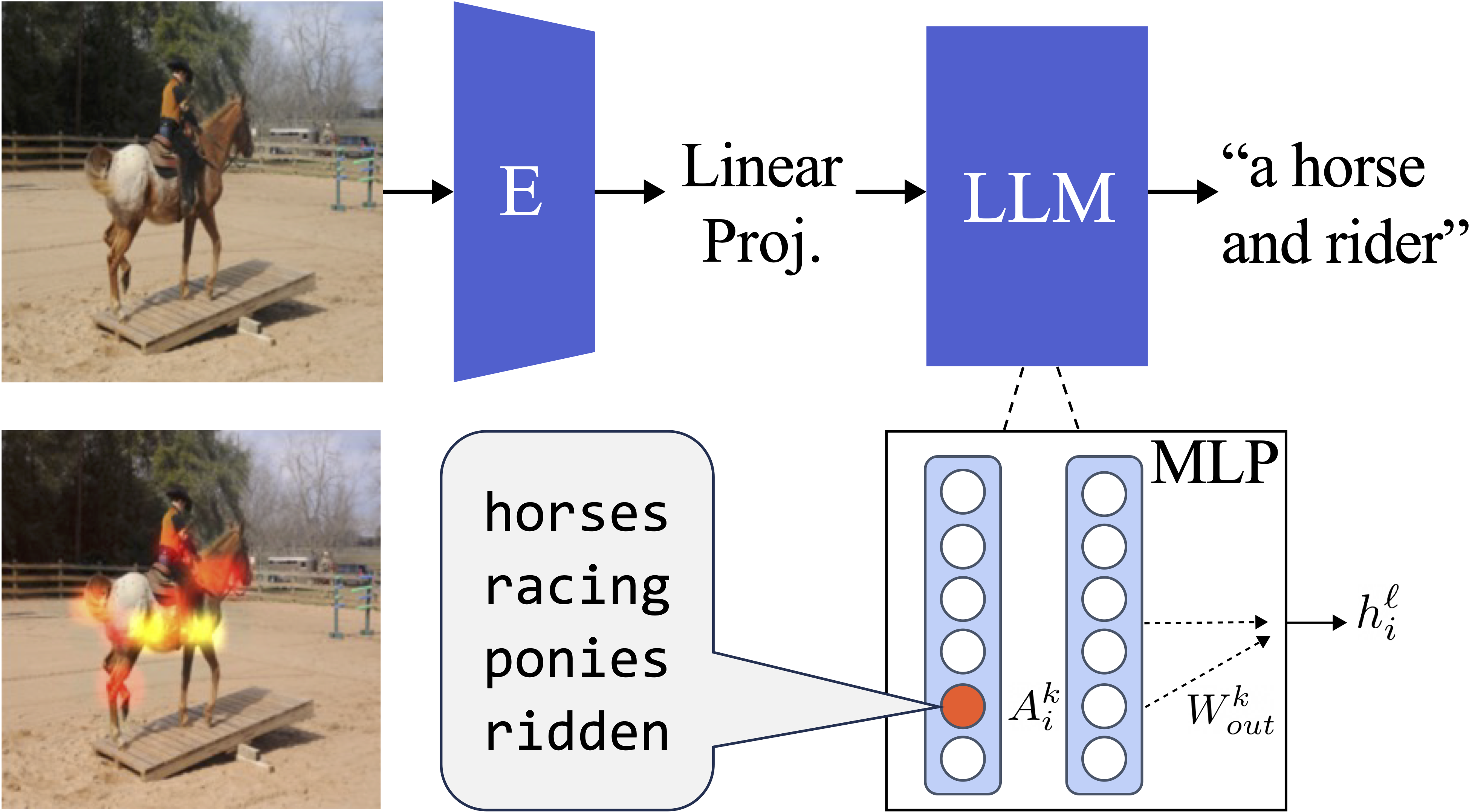
Figure 1: Multimodal neurons in transformer MLPs activate on specific image features and inject related text into the model’s next token prediction. Unit 2019 in GPT-J layer 14 detects horses.

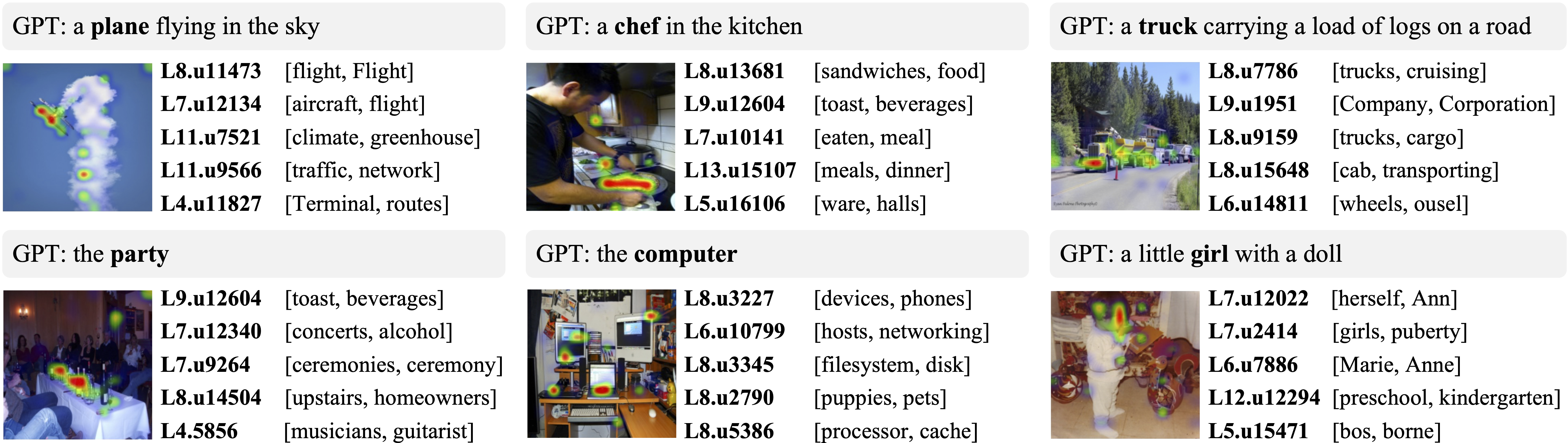
Figure 2: Top five multimodal neurons (layer L, unit u), for sample images from 6 COCO supercategories. Superimposed heatmaps ($0.95$ percentile of activations) show mean activations of the top five neurons over the image. Gradient-based attribution scores are computed with respect to the logit shown in bold in the GPT caption of each image. The two highest-probability tokens are shown for each neuron.

Vision-language models commonly employ an image-conditioned variant of prefix-tuning [20, 22], where a separate image encoder is aligned to a text decoder with a learned adapter layer. While Frozen [40], MAGMA [7], and FROMAGe [18] all use image encoders such as CLIP [33] trained jointly with language, the recent LiMBeR [28] study includes a unique setting: one experiment uses the self-supervised BEIT [2] network, trained with no linguistic supervision, and a linear projection layer between BEIT and GPT-J [43] supervised by an image-to-text task. This setting is the machine analogue of the Molyneux scenario: the major text components have never seen an image, and the major image components have never seen a piece of text, yet LiMBeR-BEIT demonstrates competitive image captioning performance [28]. To account for the transfer of semantics between modalities, are visual inputs translated into related text by the projection layer, or does alignment of vision and language representations happen inside the text transformer? In this work, we find:

1. Image prompts cast into the transformer embedding space do not encode interpretable semantics. Translation between modalities occurs inside the transformer.

2. Multimodal neurons can be found within the transformer, and they are active in response to particular image semantics.

3. Multimodal neurons causally affect output: modulating them can remove concepts from image captions.

2 Multimodal Neurons

Investigations of individual units inside deep networks have revealed a range of human-interpretable functions: for example, color-detectors and Gabor filters emerge in low-level convolutional units in image classifiers [8], and later units that activate for object categories have been found across vision architectures and tasks [44, 3, 31, 5, 16]. Multimodal neurons selective for images and text with similar semantics have previously been identified by Goh et al. [12] in the CLIP [33] visual encoder, a ResNet-50 model [14] trained to align image-text pairs. In this work, we show that multimodal neurons also emerge when vision and language are learned entirely separately, and convert visual representations aligned to a frozen language model into text.

2.1 Detecting multimodal neurons

We analyze text transformer neurons in the multimodal LiMBeR model [28], where a linear layer trained on CC3M [36] casts BEIT [2] image embeddings into the input space ($e_{L}=4096$) of GPT-J 6B [43]. GPT-J transforms input sequence $x=[x_{1},\dots,x_{P}]$ into a probability distribution $y$ over next-token continuations of $x$ [42], to create an image caption (where $P=196$ image patches). At layer $\ell$, the hidden state $h_{i}^{\ell}$ is given by $h_{i}^{\ell-1}+\mathbf{a_{i}}^{\ell}+\mathbf{m_{i}}^{\ell}$, where $\mathbf{a_{i}}^{\ell}$ and $\mathbf{m_{i}}^{\ell}$ are attention and MLP outputs. The output of the final layer $L$ is decoded using $W_{d}$ for unembedding: $y=\mathrm{softmax}(W_{d}h^{L})$, which we refer to as $~{}\mathrm{decoder}(h^{L})$.

Recent work has found that transformer MLPs encode discrete and recoverable knowledge attributes  [11, 6, 26, 27]. Each MLP is a two-layer feedforward neural network that, in GPT-J, operates on $h_{i}^{\ell-1}$ as follows:

$$\mathbf{m_{i}}^{\ell}=W^{\ell}_{out}\mathrm{GELU}(W^{\ell}_{in}h_{i}^{\ell-1})$$ (1)

Motivated by past work uncovering interpretable roles of individual MLP neurons in language-only settings [6], we investigate their function in a multimodal context.

Attributing model outputs to neurons with image input.

We apply a procedure based on gradients to evaluate the contribution of neuron $u_{k}$ to an image captioning task. This approach follows several related approaches in neuron attribution, such as Grad-CAM  [35] and Integrated Gradients  [39, 6]. We adapt to the recurrent nature of transformer token prediction by attributing generated tokens in the caption to neuron activations, which may be several transformer passes earlier. We assume the model is predicting $c$ as the most probable next token $t$, with logit $y^{c}$. We define the attribution score $g$ of $u_{k}$ on token $c$ after a forward pass through image patches $\{1,\dots,p\}$ and pre-activation output $Z$, using the following equation:

$$g_{k,c}=Z^{k}_{p}\frac{\partial y^{c}}{\partial Z^{k}_{p}}$$ (2)

This score is maximized when both the neuron’s output and the effect of the neuron are large. It is a rough heuristic, loosely approximating to first-order the neuron’s effect on the output logit, compared to a baseline in which the neuron is ablated. Importantly, this gradient can be computed efficiently for all neurons using a single backward pass.

2.2 Decoding multimodal neurons

What effect do neurons with high $g_{k,c}$ have on model output? We consider $u_{k}\in U^{\ell}$, the set of first-layer MLP units ($|U^{\ell}|=16384$ in GPT-J). Following Equation 1 and the formulation of transformer MLPs as key-value pairs from [11], we note that activation $A_{i}^{k}$ of $u_{k}$ contributes a “value” from $W_{out}$ to $h_{i}$. After the first layer operation:

$$\mathbf{m_{i}}=W_{out}A_{i}$$ (3)

As $A_{i}^{k}$ grows relative to $A_{i}^{j}$ (where $j\neq k$), the direction of $\mathbf{m_{i}}$ approaches $W_{out}^{k}A_{i}^{k}$, where $W_{out}^{k}$ is one row of weight matrix $W_{out}$. As this vector gets added to the residual stream, it has the effect of boosting or demoting certain next-word predictions (see Figure 1). To decode the language contribution of $u_{k}$ to model output, we can directly compute $\mathrm{decoder}(W_{out}^{k})$, following the simplifying assumption that representations at any layer can be transformed into a distribution over the token vocabulary using the output embeddings [11, 10, 1, 34]. To evaluate whether $u_{k}$ translates an image representation into semantically related text, we compare $\mathrm{decoder}(W_{out}^{k})$ to image content.

	BERTScore	CLIPScore
random	.3627	21.74
multimodal neurons	.3848	23.43
GPT captions	.5251	23.62

Table 1: Language descriptions of multimodal neurons correspond with image semantics and human annotations of images. Scores are reported for a random subset of 1000 COCO validation images. Each BERTScore (F1) is a mean across 5 human image annotations from COCO. For each image, we record the max CLIPScore and BERTScore per neuron, and report means across all images.

Do neurons translate image semantics into related text?

We evaluate the agreement between visual information in an image and the text multimodal neurons inject into the image caption. For each image in the MSCOCO-2017 [23] validation set, where LiMBeR-BEIT produces captions on par with using CLIP as a visual encoder [28], we calculate $g_{k,c}$ for $u_{k}$ across all layers with respect to the first noun $c$ in the generated caption. For the $100$ $u_{k}$ with highest $g_{k,c}$ for each image, we compute $\mathrm{decoder}(W_{out}^{k})$ to produce a list of the $10$ most probable language tokens $u_{k}$ contributes to the image caption. Restricting analyses to interpretable neurons (where at least 7 of the top 10 tokens are words in the English dictionary containing $\geq$ 3 letters) retains 50% of neurons with high $g_{k,c}$ (see examples and further implementation details in the Supplement).

We measure how well decoded tokens (e.g. horses, racing, ponies, ridden, $\dots$ in Figure 1) correspond with image semantics by computing CLIPScore [17] relative to the input image and BERTScore [45] relative to COCO image annotations (e.g. a cowboy riding a horse). Table 1 shows that tokens decoded from multimodal neurons perform competitively with GPT image captions on CLIPScore, and outperform a baseline on BERTScore where pairings between images and decoded multimodal neurons are randomized (we introduce this baseline as we do not expect BERTScores for comma-separated token lists to be comparable to GPT captions, e.g. a horse and rider).

Figure 2 shows example COCO images alongside top-scoring multimodal neurons per image, and image regions where the neurons are maximally active. Most top-scoring neurons are found between layers $5$ and $10$ of GPT-J ($L=28$; see Supplement), consistent with the finding from [26] that MLP knowledge contributions occur in earlier layers.

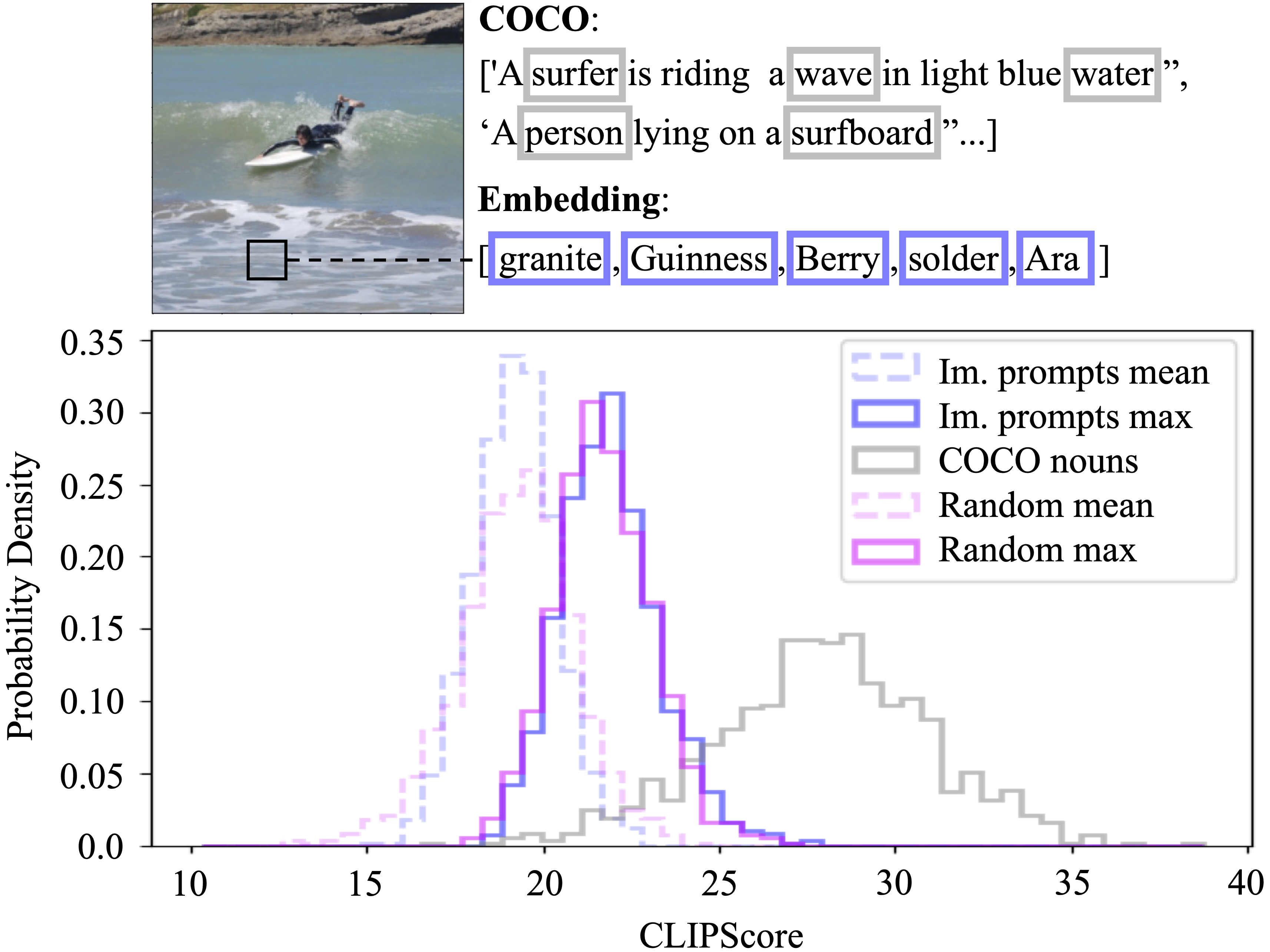
Figure 3: CLIPScores for text-image pairs show no significant difference between decoded image prompts and random embeddings. For image prompts, we report the mean across all image patches as well as the distribution of max CLIPScores per image.

	Random	Prompts	GPT	COCO
CLIPScore	19.22	19.17	23.62	27.89
BERTScore	.3286	.3291	.5251	.4470

Table 2: Image prompts are insignificantly different from randomly sampled prompts on CLIPScore and BERTScore. Scores for GPT captions and COCO nouns are shown for comparison.

3 Experiments

3.1 Does the projection layer translate images into semantically related tokens?

We decode image prompts aligned to the GPT-J embedding space into language, and measure their agreement with the input image and its human annotations for 1000 randomly sampled COCO images. As image prompts correspond to vectors in the embedding space and not discrete language tokens, we map them (and 1000 randomly sampled vectors for comparison) onto the five nearest tokens for analysis (see Figure 3 and Supplement). A Kolmogorov-Smirnov test [19, 37] shows no significant difference ($D=.037,p>.5$) between CLIPScore distributions comparing real decoded prompts and random embeddings to images. We compute CLIPScores for five COCO nouns per image (sampled from human annotations) which show significant difference ($D>.9,p<.001$) from image prompts.

We measure agreement between decoded image prompts and ground-truth image descriptions by computing BERTScores relative to human COCO annotations. Table 2 shows mean scores for real and random embeddings alongside COCO nouns and GPT captions. Real and random prompts are negligibly different, confirming that inputs to GPT-J do not readily encode interpretable semantics.

3.2 Is visual specificity robust across inputs?

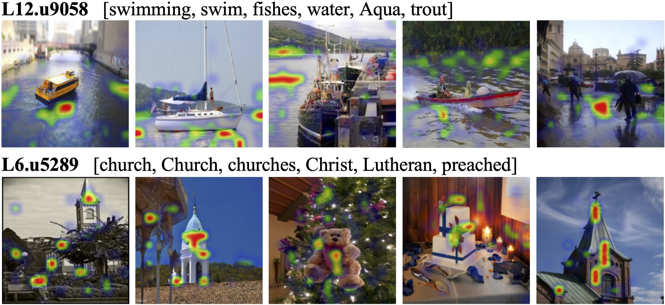
Figure 4: Top-activating COCO images for two multimodal neurons. Heatmaps ($0.95$ percentile of activations) illustrate consistent selectivity for image regions translated into related text.

A long line of interpretability research has shown that evaluating alignment between individual units and semantic concepts in images is useful for characterizing feature representations in vision models [4, 5, 46, 16]. Approaches based on visualization and manual inspection (see Figure 4) can reveal interesting phenomena, but scale poorly.

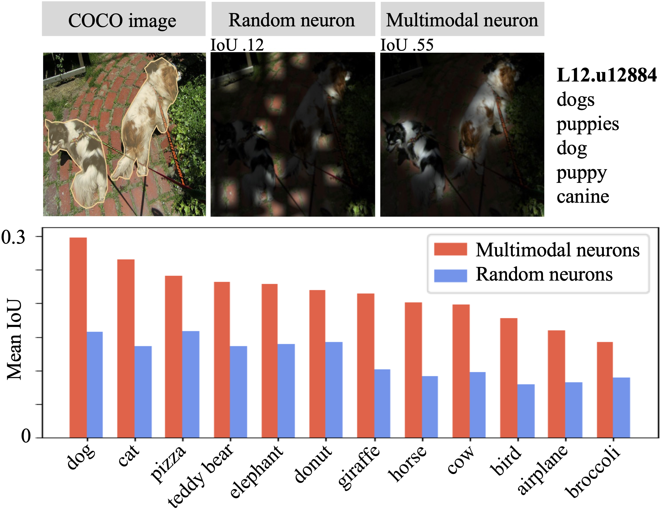
Figure 5: Across 12 COCO categories, the receptive fields of multimodal neurons better segment the concept in each image than randomly sampled neurons in the same layers. The Supplement provides additional examples.

We quantify the selectivity of multimodal neurons for specific visual concepts by measuring the agreement of their receptive fields with COCO instance segmentations, following [3]. We simulate the receptive field of $u_{k}$ by computing $A_{i}^{k}$ on each image prompt $x_{i}\in[x_{1},...,x_{P}]$, reshaping $A_{i}^{k}$ into a $14\times 14$ heatmap, and scaling to $224\times 224$ using bilinear interpolation. We then threshold activations above the $0.95$ percentile to produce a binary mask over the image, and compare this mask to COCO instance segmentations using Intersection over Union (IoU). To test specificity for individual objects, we select 12 COCO categories with single object annotations, and show that across all categories, the receptive fields of multimodal neurons better segment the object in each image than randomly sampled neurons from the same layers (Figure 5). While this experiment shows that multimodal neurons are reliable detectors of concepts, we also test whether they are selectively active for images containing those concepts, or broadly active across images. Results in the Supplement show preferential activation on particular categories of images.

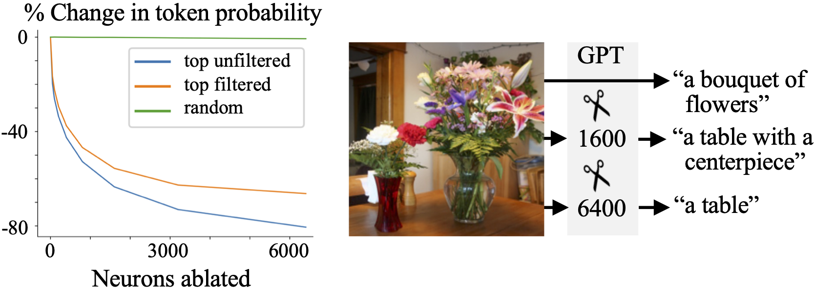
Figure 6: Ablating multimodal neurons degrades image caption content. We plot the effect of ablating multimodal neurons ordered by $g_{k,c}$ and randomly sampled units in the same layers (left), and show an example (right) of the effect on a single image caption.

3.3 Do multimodal neurons causally affect output?

To investigate how strongly multimodal neurons causally affect model output, we successively ablate units sorted by $g_{k,c}$ and measure the resulting change in the probability of token $c$. Results for all COCO validation images are shown in Figure 6, for multimodal neurons (filtered and unfiltered for interpretability), and randomly selected units in the same layers. When up to 6400 random units are ablated, we find that the probability of token $c$ is largely unaffected, but ablating the same number of top-scoring units decreases token probability by 80% on average. Ablating multimodal neurons also leads to significant changes in the semantics of GPT-generated captions. Figure 6 shows one example; additional analysis is provided in the Supplement.

4 Conclusion

We find multimodal neurons in text-only transformer MLPs and show that these neurons consistently translate image semantics into language. Interestingly, soft-prompt inputs to the language model do not map onto interpretable tokens in the output vocabulary, suggesting translation between modalities happens inside the transformer. The capacity to align representations across modalities could underlie the utility of language models as general-purpose interfaces for tasks involving sequential modeling [25, 13, 38, 29], ranging from next-move prediction in games [21, 32] to protein design [41, 9]. Understanding the roles of individual computational units can serve as a starting point for investigating how transformers generalize across tasks.

5 Limitations

We study a single multimodal model (LiMBeR-BEIT) of particular interest because the vision and language components were learned separately. The discovery of multimodal neurons in this setting motivates investigation of this phenomenon in other vision-language architectures, and even models aligning other modalities. Do similar neurons emerge when the visual encoder is replaced with a raw pixel stream such as in [25], or with a pretrained speech autoencoder? Furthermore, although we found that the outputs of the LiMBeR-BEIT projection layer are not immediately decodable into interpretable language, our knowledge of the structure of the vector spaces that represent information from different modalities remains incomplete, and we have not investigated how concepts encoded by individual units are assembled from upstream representations. Building a more mechanistic understanding of information processing within transfomers may help explain their surprising ability to generalize to non-textual representations.

6 Acknowledgements

We are grateful for the support of the MIT-IBM Watson AI Lab, and ARL grant W911NF-18-2-0218. We thank Jacob Andreas, Achyuta Rajaram, and Tazo Chowdhury for their useful input and insightful discussions.

Supplemental Material for Multimodal Neurons in Pretrained Text-Only Transformers

S.1 Implementation details

We follow the LiMBeR process for augmenting pretrained GPT-J with vision as described in Merullo et al. (2022). Each image is resized to $(224,224)$ and encoded into a sequence $[i_{1},...,i_{k}]$ by the image encoder $E$, where $k=196$ and each $i$ corresponds to an image patch of size $(16,16)$. We use self-supervised BEIT as $E$, trained with no linguistic supervision, which produces $[i_{1},...,i_{k}]$ of dimensionality $1024$. To project image representations $i$ into the transformer-defined embedding space of GPT-J, we use linear layer $P$ from Merullo et al. (2022), trained on an image-to-text task (CC3M image captioning). $P$ transforms $[i_{1},...,i_{k}]$ into soft prompts $[x_{1},...,x_{k}]$ of dimensionality $4096$, which we refer to as the image prompt. Following convention from SimVLM, MAGMA and LiMBeR, we append the text prefix “A picture of” after every every image prompt. Thus for each image, GPT-J receives as input a $(199,4096)$ prompt and outputs a probability distribution $y$ over next-token continuations of that prompt.

To calculate neuron attribution scores, we generate a caption for each image by sampling from $y$ using temperature $T=0$, which selects the token with the highest probability at each step. The attribution score $g_{k,c}$ of neuron $k$ is then calculated with respect to token $c$, where $c$ is the first noun in the generated caption (which directly follows the image prompt and is less influenced by earlier token predictions). In the rare case where this noun is comprised of multiple tokens, we let $c$ be the first of these tokens. This attribution score lets us rank multimodal neurons by how much they contribute to the crossmodal image captioning task.

S.2 Example multimodal neurons

Table S.1 shows additional examples of multimodal neurons detected and decoded for randomly sampled images from the COCO 2017 validation set. The table shows the top 20 neurons across all MLP layers for each image. In analyses where we filter for interpretable neurons that correspond to objects or object features in images, we remove neurons that decode primarily to word fragments or punctuation. Interpretable units (units where at least 7 of the top 10 tokens are words in the SCOWL English dictionary, for en-US or en-GB, with $\geq 3$ letters) are highlighted in bold.

S.3 Evaluating agreement with image captions

We use BERTScore (F1) as a metric for evaluating how well a list of tokens corresponds to the semantic content of an image caption. Section 2.2 uses this metric to evaluate multimodal neurons relative to ground-truth human annotations from COCO, and Section 3.1 uses the metric to determine whether projection layer $P$ translates $[i_{1},...,i_{k}]$ into $[x_{1},...,x_{k}]$ that already map visual features onto related language before reaching transformer MLPs. Given that $[x_{1},...,x_{k}]$ do not correspond to discrete tokens, we map each $x$ onto the $5$ token vectors with highest cosine similarity in the transformer embedding space for analysis.

Table S.2 shows example decoded soft prompts for a randomly sampled COCO image. For comparison, we sample random vectors of size $4096$ and use the same procedure to map them onto their nearest neighbors in the GPT-J embedding space. BERTScores for the random soft prompts are shown alongside scores for the image soft prompts. The means of these BERTScores, as well as the maximum values, are indistinguishable for real and random soft prompts (see Table S.2 for a single image and Figure 3 in the main paper for the distribution across COCO images). Thus we conclude that $P$ produces image prompts that fit within the GPT-J embedding space, but do not already map image features onto related language: this occurs deeper inside the transformer.

S.4 Selectivity of multimodal neurons

Figure S.1 shows additional examples of activation masks of individual multimodal neurons over COCO validation images, and IoU scores comparing each activation mask with COCO object annotations.

We conduct an additional experiment to test whether multimodal neurons are selectively active for images containing particular concepts. If unit $k$ is selective for the images it describes (and not, for instance, for many images), then we expect greater $A^{k}_{x_{i}}$ on images where it relevant to the caption than on images where it is irrelevant. It is conceivable that our method merely extracts a set of high-activating neurons, not a set of neurons that are selectively active on the inputs we claim they are relevant to captioning.

We select 10 diverse ImageNet classes (see Figure S.2) and compute the top 100 scoring units per image on each of 200 randomly sampled images per class in the ImageNet training set, filtered for interpretable units. Then for each class, we select the 20 units that appear in the most images for that class. We measure the mean activation of these units across all patches in the ImageNet validation images for each of the 10 classes. Figure S.2(a) shows the comparison of activations across each of the categories. We find that neurons activate more frequently on images in their own category than for others. This implies that our pipeline does not extract a set of general visually attentive units, but rather units that are specifically tied to image semantics.

Images	Layer.unit	Patch	Decoding (top 5 tokens)	Attr. score
	L7.u15772	119	‘ animals’, ‘ embryos’, ‘ kittens’, ‘ mammals’, ‘ eggs’	0.0214
	L5.u4923	119	‘ birds’, ‘ cages’, ‘ species’, ‘ breeding’, ‘ insects’	0.0145
	L7.u12134	119	‘ aircraft’, ‘ flight’, ‘ airplanes’, ‘ Flight’, ‘ Aircraft’	0.0113
	L5.u4888	119	‘ Boat’, ‘ sails’, ‘voy’, ‘ boats’, ‘ ships’	0.0085
	L7.u5875	119	‘ larvae’, ‘ insects’, ‘ mosquitoes’, ‘ flies’, ‘ species’	0.0083
	L8.u2012	105	‘ whales’, ‘ turtles’, ‘ whale’, ‘ birds’, ‘ fishes’	0.0081
	L7.u3030	119	‘ Island’, ‘ island’, ‘ Islands’, ‘ islands’, ‘ shore’	0.0078
	L7.u14308	119	‘uses’, ‘ dec’, ‘bill’, ‘oid’, ‘FS’	0.0078
	L9.u12771	119	‘ satellites’, ‘ Flight’, ‘ orbiting’, ‘ spacecraft’, ‘ ship’	0.0075
	L4.u12317	119	‘ embryos’, ‘ chicken’, ‘ meat’, ‘ fruits’, ‘ cows’	0.0071
	L8.u2012	119	‘ whales’, ‘ turtles’, ‘ whale’, ‘ birds’, ‘ fishes’	0.0062
	L5.u4530	119	‘ herds’, ‘ livestock’, ‘ cattle’, ‘ herd’, ‘ manure’	0.0056
	L5.u4923	105	‘ birds’, ‘ cages’, ‘ species’, ‘ breeding’, ‘ insects’	0.0055
	L6.u8956	119	‘ virus’, ‘ strains’, ‘ infect’, ‘ viruses’, ‘ parasites’	0.0052
	L7.u2159	105	‘ species’, ‘species’, ‘ bacteria’, ‘ genus’, ‘ Species’	0.0051
	L10.u4819	119	‘çĶ°’, ‘¬¼’, ‘”””’, ‘ Marketable’, ‘姒	0.0051
	L5.u4923	118	‘ birds’, ‘ cages’, ‘ species’, ‘ breeding’, ‘ insects’	0.0050
	L10.u927	3	‘onds’, ‘rog’, ‘lys’, ‘arrow’, ‘ond’	0.0050
	L11.u7635	119	‘ birds’, ‘birds’, ‘ butterflies’, ‘ kittens’, ‘ bird’	0.0049
	L9.u15445	119	‘ radar’, ‘ standby’, ‘ operational’, ‘ flight’, ‘ readiness’	0.0048
	L5.u15728	119	‘ playoff’, ‘ players’, ‘ teammate’, ‘ player’, ‘Players’	0.0039
	L12.u11268	113	‘elson’, ‘ISA’, ‘Me’, ‘PRES’, ‘SO’	0.0039
	L5.u9667	119	‘ workouts’, ‘ workout’, ‘ Training’, ‘ trainer’, ‘ exercises’	0.0034
	L9.u15864	182	‘lihood’, ‘/**’, ‘Advertisements’, ‘.”.’, ‘”””’	0.0034
	L9.u9766	119	‘ soccer’, ‘ football’, ‘ player’, ‘ baseball’, ‘player’	0.0033
	L10.u4819	182	‘çĶ°’, ‘¬¼’, ‘”””’, ‘ Marketable’, ‘姒	0.0033
	L18.u15557	150	‘imer’, ‘ohan’, ‘ellow’, ‘ims’, ‘gue’	0.0032
	L12.u6426	160	‘⢒, ‘ ®’, ‘ syndrome’, ‘ Productions’, ‘ Ltd’	0.0032
	L8.u15435	119	‘ tennis’, ‘ tournaments’, ‘ tournament’, ‘ golf’, ‘ racing’	0.0032
	L11.u4236	75	‘ starring’, ‘ played’, ‘ playable’, ‘ Written’, ‘ its’	0.0031
	L8.u6207	119	‘ player’, ‘ players’, ‘ Player’, ‘Ä’, ‘ talent’	0.0031
	L6.u5975	119	‘ football’, ‘ soccer’, ‘ basketball’, ‘ Soccer’, ‘ Football’	0.0030
	L2.u10316	75	‘ï’, ‘/**’, ‘Q’, ‘The’, ‘//’	0.0028
	L12.u8390	89	‘etheless’, ‘viously’, ‘theless’, ‘bsite’, ‘terday’	0.0028
	L5.u7958	89	‘ rugby’, ‘ football’, ‘ player’, ‘ soccer’, ‘ footballer’	0.0028
	L20.u9909	89	‘ Associates’, ‘ Alt’, ‘ para’, ‘ Lt’, ‘ similarly’	0.0026
	L5.u8219	75	‘ portion’, ‘ regime’, ‘ sector’, ‘ situation’, ‘ component’	0.0026
	L11.u7264	75	‘ portion’, ‘ finale’, ‘ environment’, ‘iest’, ‘ mantle’	0.0026
	L20.u452	103	‘ CLE’, ‘ plain’, ‘ clearly’, ‘ Nil’, ‘ Sullivan’	0.0026
	L7.u16050	89	‘pc’, ‘IER’, ‘ containing’, ‘ formatted’, ‘ supplemented’	0.0026
	L10.u927	73	‘onds’, ‘rog’, ‘lys’, ‘arrow’, ‘ond’	0.0087
	L5.u9667	101	‘ workouts’, ‘ workout’, ‘ Training’, ‘ trainer’, ‘ exercises’	0.0081
	L9.u3561	73	‘ mix’, ‘ CRC’, ‘ critically’, ‘ gulf’, ‘ mechanically’	0.0076
	L9.u5970	73	‘ construct’, ‘ performance’, ‘ global’, ‘ competing’, ‘ transact’	0.0054
	L10.u562	73	‘ prev’, ‘ struct’, ‘ stable’, ‘ marg’, ‘ imp’	0.0054
	L6.u14388	87	‘ march’, ‘ treadmill’, ‘ Championships’, ‘ racing’, ‘ marathon’	0.0052
	L14.u10320	73	‘ print’, ‘ handle’, ‘ thing’, ‘catch’, ‘error’	0.0051
	L9.u3053	73	‘essel’, ‘ked’, ‘ ELE’, ‘ument’, ‘ue’	0.0047
	L5.u4932	73	‘eman’, ‘rack’, ‘ago’, ‘anne’, ‘ison’	0.0046
	L9.u7777	101	‘dr’, ‘thur’, ‘tern’, ‘mas’, ‘mass’	0.0042
	L6.u16106	73	‘umble’, ‘archives’, ‘room’, ‘ decentral’, ‘Root’	0.0040
	L5.u14519	73	‘ abstract’, ‘ global’, ‘map’, ‘exec’, ‘kernel’	0.0039
	L11.u10405	73	‘amed’, ‘elect’, ‘1’, ‘vol’, ‘vis’	0.0038
	L9.u325	87	‘ training’, ‘ tournaments’, ‘ango’, ‘ ballet’, ‘ gymn’	0.0038
	L6.u14388	101	‘ march’, ‘ treadmill’, ‘ Championships’, ‘ racing’, ‘ marathon’	0.0038
	L7.u3844	101	‘DERR’, ‘Charges’, ‘wana’, ‘¬¼’, ‘verages’	0.0036
	L9.u15864	101	‘lihood’, ‘/**’, ‘Advertisements’, ‘.”.’, ‘”””’	0.0036
	L7.u3330	101	‘ Officers’, ‘ officers’, ‘ patrolling’, ‘ patrols’, ‘ troops’	0.0036
	L8.u8807	73	‘ program’, ‘ updates’, ‘ programs’, ‘ document’, ‘ format’	0.0034
	L6.u12536	87	‘ ankles’, ‘ joints’, ‘ biome’, ‘ injuries’, ‘ injury’	0.0034

Images	Layer.unit	Patch	Decoding (top 5 tokens)	Attr. score
	L8.u14504	13	‘ upstairs’, ‘ homeowners’, ‘ apartments’, ‘ houses’, ‘ apartment’	0.0071
	L13.u15107	93	‘ meals’, ‘ meal’, ‘ dinner’, ‘ dishes’, ‘ cuisine’	0.0068
	L8.u14504	93	‘ upstairs’, ‘ homeowners’, ‘ apartments’, ‘ houses’, ‘ apartment’	0.0052
	L8.u14504	150	‘ upstairs’, ‘ homeowners’, ‘ apartments’, ‘ houses’, ‘ apartment’	0.0048
	L9.u4691	13	‘ houses’, ‘ buildings’, ‘ dwellings’, ‘ apartments’, ‘ homes’	0.0043
	L8.u13681	93	‘ sandwiches’, ‘ foods’, ‘ salad’, ‘ sauce’, ‘ pizza’	0.0041
	L12.u4638	93	‘ wash’, ‘ Darkness’, ‘ Caps’, ‘ blush’, ‘ Highest’	0.0040
	L9.u3561	93	‘ mix’, ‘ CRC’, ‘ critically’, ‘ gulf’, ‘ mechanically’	0.0040
	L7.u5533	93	‘bags’, ‘Items’, ‘ comprehens’, ‘ decor’, ‘bag’	0.0039
	L9.u8687	93	‘ eaten’, ‘ foods’, ‘ food’, ‘ diet’, ‘ eating’	0.0037
	L12.u4109	93	‘ Lakes’, ‘ Hof’, ‘ Kass’, ‘ Cotton’, ‘Council’	0.0036
	L8.u943	93	‘ Foods’, ‘Food’, ‘let’, ‘ lunch’, ‘commercial’	0.0036
	L5.u16106	93	‘ware’, ‘ halls’, ‘ salt’, ‘WARE’, ‘ mat’	0.0032
	L8.u14504	143	‘ upstairs’, ‘ homeowners’, ‘ apartments’, ‘ houses’, ‘ apartment’	0.0032
	L9.u11735	93	‘ hysterical’, ‘ Gould’, ‘ Louie’, ‘ Gamble’, ‘ Brown’	0.0031
	L8.u14504	149	‘ upstairs’, ‘ homeowners’, ‘ apartments’, ‘ houses’, ‘ apartment’	0.0031
	L5.u2771	93	‘ occupations’, ‘ industries’, ‘ operations’, ‘ occupational’, ‘ agriculture’	0.0029
	L9.u15864	55	‘lihood’, ‘/**’, ‘Advertisements’, ‘.”.’, ‘”””’	0.0028
	L9.u4691	149	‘ houses’, ‘ buildings’, ‘ dwellings’, ‘ apartments’, ‘ homes’	0.0028
	L7.u10853	13	‘ boutique’, ‘ firm’, ‘ Associates’, ‘ restaurant’, ‘ Gifts’	0.0028
	L8.u15435	160	‘ tennis’, ‘ tournaments’, ‘ tournament’, ‘ golf’, ‘ racing’	0.0038
	L1.u15996	132	‘276’, ‘PS’, ‘ley’, ‘room’, ‘ Will’	0.0038
	L5.u6439	160	‘ ge’, ‘ fibers’, ‘ hair’, ‘ geometric’, ‘ ori’	0.0037
	L9.u15864	160	‘lihood’, ‘/**’, ‘Advertisements’, ‘.”.’, ‘”””’	0.0034
	L12.u2955	160	‘Untitled’, ‘Welcome’, ‘========’, ‘Newsletter’, ‘====’	0.0033
	L12.u2955	146	‘Untitled’, ‘Welcome’, ‘========’, ‘Newsletter’, ‘====’	0.0032
	L7.u2688	160	‘rection’, ‘itud’, ‘ Ratio’, ‘lat’, ‘ ratio’	0.0031
	L8.u4372	160	‘ footage’, ‘ filmed’, ‘ filming’, ‘ videos’, ‘ clips’	0.0029
	L10.u4819	146	‘çĶ°’, ‘¬¼’, ‘”””’, ‘ Marketable’, ‘姒	0.0029
	L8.u15435	93	‘ tennis’, ‘ tournaments’, ‘ tournament’, ‘ golf’, ‘ racing’	0.0029
	L8.u15435	146	‘ tennis’, ‘ tournaments’, ‘ tournament’, ‘ golf’, ‘ racing’	0.0029
	L10.u927	132	‘onds’, ‘rog’, ‘lys’, ‘arrow’, ‘ond’	0.0027
	L9.u15864	146	‘lihood’, ‘/**’, ‘Advertisements’, ‘.”.’, ‘”””’	0.0026
	L1.u8731	132	‘ âĢ¦’, ‘ [âĢ¦]’, ‘âĢ¦’, ‘ …’, ‘ Will’	0.0025
	L8.u16330	160	‘ bouncing’, ‘ hitting’, ‘ bounce’, ‘ moving’, ‘ bounced’	0.0025
	L9.u1908	146	‘ members’, ‘ country’, ‘ VIII’, ‘ Spanish’, ‘ 330’	0.0024
	L10.u4819	160	‘çĶ°’, ‘¬¼’, ‘”””’, ‘ Marketable’, ‘姒	0.0024
	L11.u14710	160	‘Search’, ‘Follow’, ‘Early’, ‘Compar’, ‘Category’	0.0024
	L6.u132	160	‘ manually’, ‘ replace’, ‘ concurrently’, ‘otropic’, ‘ foregoing’	0.0024
	L7.u5002	160	‘ painting’, ‘ paintings’, ‘ sculpture’, ‘ sculptures’, ‘ painted’	0.0024

Images	Layer.unit	Patch	Decoding (top 5 tokens)	Attr. score
	L5.u13680	132	‘ driver’, ‘ drivers’, ‘ cars’, ‘heading’, ‘cars’	0.0091
	L11.u9566	132	‘ traffic’, ‘ network’, ‘ networks’, ‘ Traffic’, ‘network’	0.0090
	L12.u11606	132	‘ chassis’, ‘ automotive’, ‘ design’, ‘ electronics’, ‘ specs’	0.0078
	L7.u6109	132	‘ automobile’, ‘ automobiles’, ‘ engine’, ‘ Engine’, ‘ cars’	0.0078
	L6.u11916	132	‘ herd’, ‘loads’, ‘ racing’, ‘ herds’, ‘ horses’	0.0071
	L8.u562	132	‘ vehicles’, ‘ vehicle’, ‘ cars’, ‘veh’, ‘ Vehicles’	0.0063
	L7.u3273	132	‘ride’, ‘ riders’, ‘ rides’, ‘ ridden’, ‘ rider’	0.0062
	L13.u5734	132	‘ Chevrolet’, ‘ Motorsport’, ‘ cars’, ‘ automotive’, ‘ vehicle’	0.0062
	L8.u2952	132	‘ rigging’, ‘ valves’, ‘ nozzle’, ‘ pipes’, ‘ tubing’	0.0059
	L13.u8962	132	‘ cruising’, ‘ flying’, ‘ flight’, ‘ refuel’, ‘ Flying’	0.0052
	L9.u3561	116	‘ mix’, ‘ CRC’, ‘ critically’, ‘ gulf’, ‘ mechanically’	0.0051
	L13.u107	132	‘ trucks’, ‘ truck’, ‘ trailer’, ‘ parked’, ‘ driver’	0.0050
	L14.u10852	132	‘Veh’, ‘ driver’, ‘ automotive’, ‘ automakers’, ‘Driver’	0.0049
	L6.u1989	132	‘text’, ‘light’, ‘TL’, ‘X’, ‘background’	0.0049
	L2.u14243	132	‘ousel’, ‘ Warriors’, ‘riages’, ‘illion’, ‘Ord’	0.0048
	L5.u6589	132	‘ vehicles’, ‘ motorcycles’, ‘ aircraft’, ‘ tyres’, ‘ cars’	0.0046
	L7.u4574	132	‘ plants’, ‘ plant’, ‘ roof’, ‘ compost’, ‘ wastewater’	0.0045
	L7.u6543	132	‘ distance’, ‘ downhill’, ‘ biking’, ‘ riders’, ‘ journeys’	0.0045
	L16.u9154	132	‘ driver’, ‘ drivers’, ‘ vehicle’, ‘ vehicles’, ‘driver’	0.0045
	L12.u7344	132	‘ commemor’, ‘ streets’, ‘ celebrations’, ‘ Streets’, ‘ highways’	0.0044
	L12.u9058	174	‘ swimming’, ‘ Swim’, ‘ swim’, ‘ fishes’, ‘ water’	0.0062
	L17.u10507	174	‘ rivers’, ‘ river’, ‘ lake’, ‘ lakes’, ‘ River’	0.0049
	L7.u3138	174	‘ basin’, ‘ ocean’, ‘ islands’, ‘ valleys’, ‘ mountains’	0.0046
	L5.u6930	149	‘ rivers’, ‘ river’, ‘ River’, ‘ waters’, ‘ waterways’	0.0042
	L7.u14218	174	‘ docks’, ‘ Coast’, ‘ swimming’, ‘ swim’, ‘melon’	0.0040
	L9.u4379	149	‘ river’, ‘ stream’, ‘ River’, ‘ Valley’, ‘ flow’	0.0038
	L6.u5868	149	‘water’, ‘ water’, ‘ waters’, ‘ river’, ‘ River’	0.0036
	L9.u4379	174	‘ river’, ‘ stream’, ‘ River’, ‘ Valley’, ‘ flow’	0.0036
	L5.u6930	174	‘ rivers’, ‘ river’, ‘ River’, ‘ waters’, ‘ waterways’	0.0032
	L7.u3138	149	‘ basin’, ‘ ocean’, ‘ islands’, ‘ valleys’, ‘ mountains’	0.0029
	L6.u5868	174	‘water’, ‘ water’, ‘ waters’, ‘ river’, ‘ River’	0.0028
	L7.u416	136	‘ praise’, ‘ glimpse’, ‘ glimps’, ‘ palate’, ‘ flavours’	0.0027
	L10.u15235	149	‘ water’, ‘ waters’, ‘water’, ‘ lake’, ‘ lakes’	0.0026
	L4.u2665	136	‘ levels’, ‘ absorbed’, ‘ density’, ‘ absorption’, ‘ equilibrium’	0.0026
	L10.u14355	149	‘ roads’, ‘ paths’, ‘ flows’, ‘ routes’, ‘ streams’	0.0026
	L17.u10507	149	‘ rivers’, ‘ river’, ‘ lake’, ‘ lakes’, ‘ River’	0.0024
	L7.u7669	174	‘ weather’, ‘ season’, ‘ forecast’, ‘ rains’, ‘ winters’	0.0024
	L8.u9322	136	‘ combustion’, ‘ turbulence’, ‘ recoil’, ‘ vibration’, ‘ hydrogen’	0.0024
	L9.u15864	182	‘lihood’, ‘/**’, ‘Advertisements’, ‘.”.’, ‘”””’	0.0022
	L7.u3138	78	‘ basin’, ‘ ocean’, ‘ islands’, ‘ valleys’, ‘ mountains’	0.0021

Table S.1: Results of attribution analysis for randomly sampled images from the COCO validation set. Includes decoded tokens for the top 20 units by attribution score. The first column shows the COCO image and superimposed heatmaps of the mean activations from the top 20 units and the top interpretable units (shown in bold). Units can repeat if they attain a high attribution score on multiple image patches.

Image	COCO Human Captions	GPT Caption
	A man riding a snowboard down the side of a snow covered slope.	A person jumping on the ice.
	A man snowboarding down the side of a snowy mountain.
	Person snowboarding down a steep snow covered slope.
	A person snowboards on top of a snowy path.
	The person holds both hands in the air while snowboarding.

Patch	Image soft prompt (nearest neighbor tokens)	BSc.	Random soft prompt (nearest neighbor tokens)	BSc.
144	[‘nav’, ‘GY’, ‘+++’, ‘done’, ‘Sets’]	.29	[‘Movement’, ‘Ord’, ‘CLUD’, ‘levy’, ‘LI’]	.31
80	[‘heels’, ‘merits’, ‘flames’, ‘platform’, ‘fledged’]	.36	[‘adic’, ‘Stub’, ‘imb’, ‘VER’, ‘stroke’]	.34
169	[‘ear’, ‘Nelson’, ‘Garden’, ‘Phill’, ‘Gun’]	.32	[‘Thank’, ‘zilla’, ‘Develop’, ‘Invest’, ‘Fair’]	.31
81	[‘vanilla’, ‘Poc’, ‘Heritage’, ‘Tarant’, ‘bridge’]	.33	[‘Greek’, ‘eph’, ‘jobs’, ‘phylogen’, ‘TM’]	.30
89	[‘oily’, ‘stant’, ‘cement’, ‘Caribbean’, ‘Nad’]	.37	[‘Forestry’, ‘Mage’, ‘Hatch’, ‘Buddh’, ‘Beaut’]	.34
124	[‘ension’, ‘ideas’, ‘GY’, ‘uler’, ‘Nelson’]	.32	[‘itone’, ‘gest’, ‘Af’, ‘iple’, ‘Dial’]	.30
5	[‘proves’, ‘Feed’, ‘meaning’, ‘zzle’, ‘stripe’]	.31	[‘multitude’, ‘psychologically’, ‘Taliban’, ‘Elf’, ‘Pakistan’]	.36
175	[‘util’, ‘elson’, ‘asser’, ‘seek’, ‘////////////////////’]	.26	[‘ags’, ‘Git’, ‘mm’, ‘Morning’, ‘Cit’]	.33
55	[‘Judicial’, ‘wasting’, ‘oen’, ‘oplan’, ‘trade’]	.34	[‘odd’, ‘alo’, ‘rophic’, ‘perv’, ‘pei’]	.34
61	[‘+++’, ‘DEP’, ‘enum’, ‘vernight’, ‘posted’]	.33	[‘Newspaper’, ‘iii’, ‘INK’, ‘Graph’, ‘UT’]	.35
103	[‘Doc’, ‘Barth’, ‘details’, ‘DEF’, ‘buckets’]	.34	[‘pleas’, ‘Eclipse’, ‘plots’, ‘cb’, ‘Menu’]	.36
99	[‘+++’, ‘Condition’, ‘Daytona’, ‘oir’, ‘research’]	.35	[‘Salary’, ‘card’, ‘mobile’, ‘Cour’, ‘Hawth’]	.35
155	[‘Named’, ‘910’, ‘collar’, ‘Lars’, ‘Cats’]	.33	[‘Champ’, ‘falsely’, ‘atism’, ‘styles’, ‘Champ’]	.30
145	[‘cer’, ‘args’, ‘olis’, ‘te’, ‘atin’]	.30	[‘Chuck’, ‘goose’, ‘anthem’, ‘wise’, ‘fare’]	.33
189	[‘MOD’, ‘Pres’, ‘News’, ‘Early’, ‘Herz’]	.33	[‘Organ’, ‘CES’, ‘POL’, ‘201’, ‘Stan’]	.31
49	[‘Pir’, ‘Pir’, ‘uum’, ‘akable’, ‘Prairie’]	.30	[‘flame’, ‘roc’, ‘module’, ‘swaps’, ‘Faction’]	.33
20	[‘ear’, ‘feed’, ‘attire’, ‘demise’, ‘peg’]	.33	[‘Chart’, ‘iw’, ‘Kirst’, ‘PATH’, ‘rhy’]	.36
110	[‘+++’, ‘Bee’, ‘limits’, ‘Fore’, ‘seeking’]	.31	[‘imped’, ‘iola’, ‘Prince’, ‘inel’, ‘law’]	.33
6	[‘SIGN’, ‘Kob’, ‘Ship’, ‘Near’, ‘buzz’]	.36	[‘Tower’, ‘767’, ‘Kok’, ‘Tele’, ‘Arbit’]	.33
46	[‘childhood’, ‘death’, ‘ma’, ‘vision’, ‘Dire’]	.36	[‘Fram’, ‘exper’, ‘Pain’, ‘ader’, ‘unprotected’]	.33
113	[‘Decl’, ‘Hide’, ‘Global’, ‘orig’, ‘meas’]	.32	[‘usercontent’, ‘OTUS’, ‘Georgia’, ‘ech’, ‘GRE’]	.32
32	[‘ideas’, ‘GY’, ‘+++’, ‘Bake’, ‘Seed’]	.32	[‘GGGGGGGG’, ‘dictators’, ‘david’, ‘ugh’, ‘BY’]	.31
98	[‘Near’, ‘Near’, ‘LIN’, ‘Bee’, ‘threat’]	.30	[‘Lavrov’, ‘Debor’, ‘Hegel’, ‘Advertisement’, ‘iak’]	.34
185	[‘ceans’, ‘Stage’, ‘Dot’, ‘Price’, ‘Grid’]	.33	[‘wholesale’, ‘Cellular’, ‘Magn’, ‘Ingredients’, ‘Magn’]	.32
166	[‘bys’, ‘767’, ‘+++’, ‘bottles’, ‘gif’]	.32	[‘Bras’, ‘discipl’, ‘gp’, ‘AR’, ‘Toys’]	.33
52	[‘Kob’, ‘Site’, ‘reed’, ‘Wiley’, ‘âĻ’]	.29	[‘THER’, ‘FAQ’, ‘ibility’, ‘ilities’, ‘twitter’]	.34
90	[‘cytok’, ‘attack’, ‘Plug’, ‘strategies’, ‘uddle’]	.32	[‘Boots’, ‘Truman’, ‘CFR’, ‘ãĤ£’, ‘Shin’]	.33
13	[‘nard’, ‘Planetary’, ‘lawful’, ‘Court’, ‘eman’]	.33	[‘Nebraska’, ‘tails’, ‘ÅŁ’, ‘DEC’, ‘Despair’]	.33
47	[‘pport’, ‘overnight’, ‘Doc’, ‘ierra’, ‘Unknown’]	.34	[‘boiling’, ‘A’, ‘Ada’, ‘itude’, ‘flawed’]	.31
19	[‘mocking’, ‘chicks’, ‘GY’, ‘ear’, ‘done’]	.35	[‘illet’, ‘severely’, ‘nton’, ‘arrest’, ‘Volunteers’]	.33
112	[‘avenue’, ‘gio’, ‘Parking’, ‘riages’, ‘Herald’]	.35	[‘griev’, ‘Swanson’, ‘Guilty’, ‘Sent’, ‘Pac’]	.32
133	[‘ãĤĬ’, ‘itto’, ‘iation’, ‘asley’, ‘Included’]	.32	[‘Purs’, ‘reproductive’, ‘sniper’, ‘instruct’, ‘Population’]	.33
102	[‘drawn’, ‘Super’, ‘gency’, ‘Type’, ‘blames’]	.33	[‘metric’, ‘Young’, ‘princip’, ‘scal’, ‘Young’]	.31
79	[‘Vand’, ‘inement’, ‘straw’, ‘ridiculous’, ‘Chick’]	.34	[‘Rez’, ‘song’, ‘LEGO’, ‘Login’, ‘pot’]	.37
105	[‘link’, ‘ede’, ‘Dunk’, ‘Pegasus’, ‘Mao’]	.32	[‘visas’, ‘Mental’, ‘verbal’, ‘WOM’, ‘nda’]	.30
	Average	.33		.33

Table S.2: Image soft prompts are indistinguishable from random soft prompts via BERTScore. Each image is encoded as a sequence of 196 soft prompts, corresponding to image patches, that serve as input to GPT-J. Here we randomly sample 35 patches for a single COCO image and map them onto nearest-neighbor tokens in transformer embedding space. BERTScore is measured relative to COCO human annotations of the same image (we report the mean score over the $5$ human captions). For comparison we sample random vectors in the transformer embedding space and compute BERTScores using the same procedure.

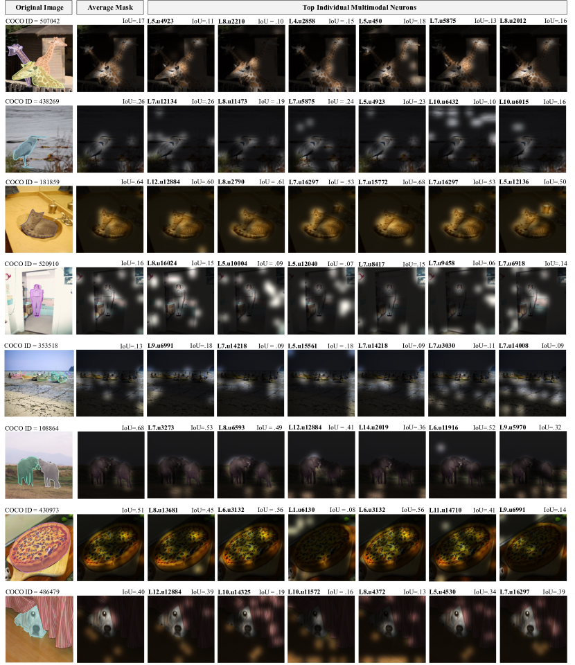
Figure S.1: Multimodal neurons are selective for objects in images. For $8$ example images sampled from the COCO categories described in Section 3.2 of the main paper, we show activation masks of individual multimodal neurons over the image, as well as mean activation masks over all top multimodal neurons. We use IoU to compare these activation masks to COCO object annotations. IoU is calculated by upsampling each activation mask to the size of the original image $(224)$ using bilinear interpolation, and thresholding activations in the 0.95 percentile to produce a binary segmentation mask.

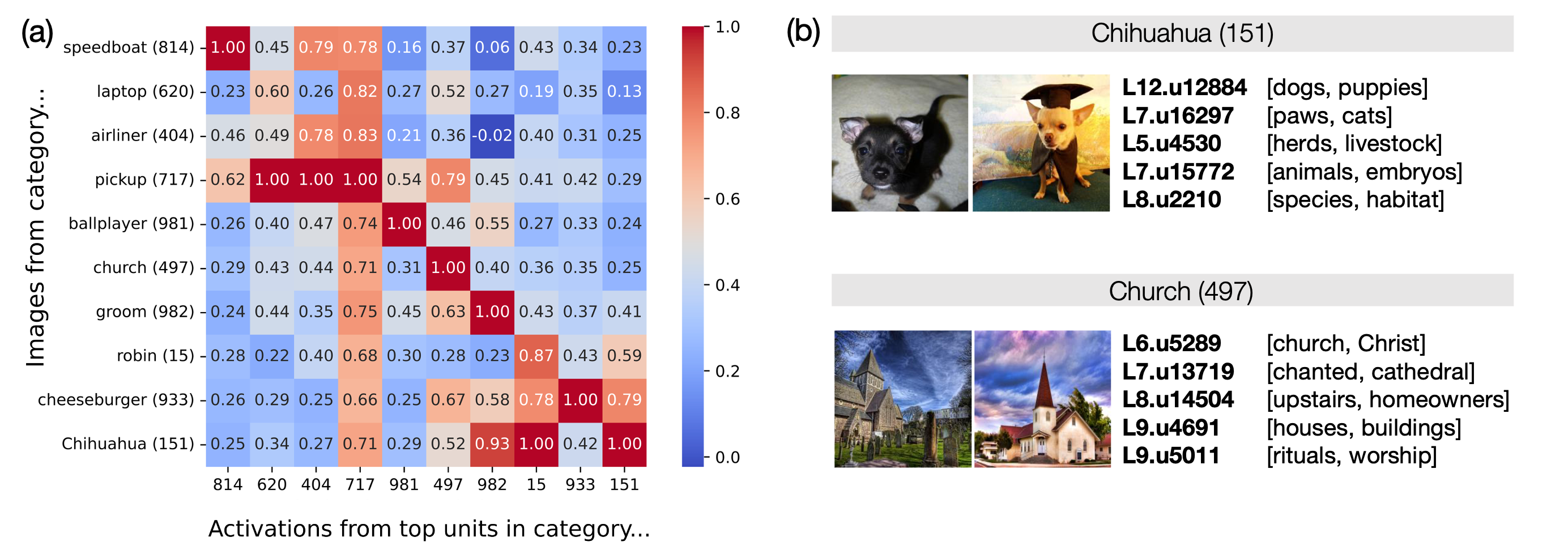
Figure S.2: Multimodal neurons are selective for image categories. (a) For 10 ImageNet classes we construct the set of interpretable multimodal neurons with the highest attribution scores on training images in that class, and calculate their activations on validation images. For each class, we report the average activation value of top-scoring multimodal units relative to the maximum value of their average activations on any class. Multimodal neurons are maximally active on classes where their attribution scores are highest. (b) Sample images and top-scoring units from two classes.

S.5 Ablating Multimodal Neurons

In Section 3.3 of the main paper, we show that ablating multimodal neurons causally effects the probability of outputting the original token. To investigate the effect of removing multimodal neurons on model output, we ablate the top $k$ units by attribution score for an image, where $k\in\{0,50,100,200,400,800,1600,3200,6400\},$ and compute the BERTScore between the model’s original caption and the newly-generated zero-temperature caption. Whether we remove the top $k$ units by attribution score, or only those that are interpretable, we observe a strong decrease in caption similarity. Table S.3 shows examples of the effect of ablating top neurons on randomly sampled COCO validation images, compared to the effect of ablating random neurons. Figure S.3 shows the average BERTScore after ablating $k$ units across all COCO validation images.

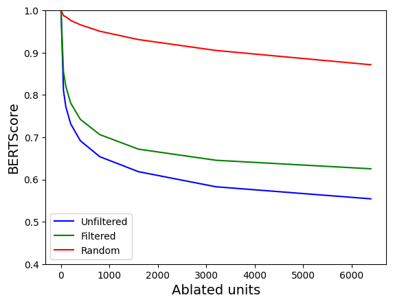
Figure S.3: BERTScores of generated captions decrease when multimodal neurons are ablated, compared to the ablation of random neurons from the same layers.

S.6 Distribution of Multimodal Neurons

We perform a simple analysis of the distribution of multimodal neurons by layer. Specifically, we extract the top 100 scoring neurons for all COCO validation images. Most of these neurons are found between layers $5$ and $10$ of GPT-J ($L=28$), suggesting translation of semantic content between modalities occurs in earlier transformer layers.

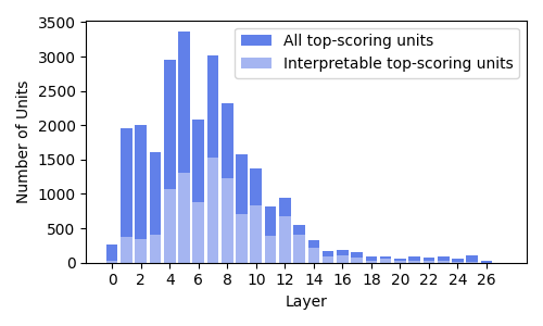
Figure S.4: Unique multimodal neurons per layer chosen using the top 100 attribution scores for each COCO validation image. Interpretable units are those for which at least 7 of the top 10 logits are words in the English dictionary containing $\geq 3$ letters.

		Captions after ablation
Img. ID	$\#$ Abl.	All multimodal	BSc.	Interpretable multimodal	BSc.	Random neurons	BSc.
219578	0	a dog with a cat	1.0	a dog with a cat	1.0	a dog with a cat	1.0
	50	a dog and a cat	.83	a dog and a cat	.83	a dog with a cat	1.0
	100	a lion and a zebra	.71	a dog and cat	.80	a dog with a cat	1.0
	200	a dog and a cat	.83	a dog and a cat	.83	a dog with a cat	1.0
	400	a lion and a lioness	.64	a dog and a cat	.83	a dog with a cat	1.0
	800	a tiger and a tiger	.63	a lion and a zebra	.71	a dog with a cat	1.0
	1600	a tiger and a tiger	.63	a lion and a zebra	.71	a dog with a cat	1.0
	3200	a tiger	.67	a tiger and a tiger	.63	a dog with a cat	1.0
	6400	a tiger	.67	a tiger in the jungle	.60	a dog with a cat	1.0
131431	0	the facade of the cathedral	1.0	the facade of the cathedral	1.0	the facade of the cathedral	1.0
	50	the facade of the church	.93	the facade of the cathedral	1.0	the facade of the cathedral	1.0
	100	the facade of the church	.93	the facade of the cathedral	1.0	the facade of the cathedral	1.0
	200	the facade	.75	the facade	.75	the facade of the cathedral	1.0
	400	the exterior of the church	.80	the facade	.75	the facade of the cathedral	1.0
	800	the exterior of the church	.80	the dome	.65	the facade of the cathedral	1.0
	1600	the dome	.65	the dome	.65	the facade of the cathedral	1.0
	3200	the dome	.65	the dome	.65	the facade of the cathedral	1.0
	6400	the exterior	.61	the dome	.65	the facade	.75
180878	0	a cake with a message		a cake with a message		a cake with a message
		written on it.	1.0	written on it.	1.0	written on it.	1.0
	50	a cake with a message		a cake with a message		a cake with a message
		written on it.	1.0	written on it.	1.0	written on it.	1.0
	100	a cake with a message		a cake for a friend’s birthday.	.59	a cake with a message
		written on it.	1.0			written on it.	1.0
	200	a cake with a message		a cake for a friend’s birthday.	.59	a cake with a message
		written on it.	1.0			written on it.	1.0
	400	a cake with a message		a cake for a friend’s birthday.	.59	a cake with a message
		written on it.	1.0			written on it.	1.0
	800	a cake	.59	a cake for a birthday party	.56	a cake with a message
						written on it.	1.0
	1600	a cake	.59	a poster for the film.	.49	a cake with a message
						written on it.	1.0
	3200	a man who is a fan of		a typewriter	.44	a cake with a message
		football	.42			written on it.	1.0
	6400	the day	.34	a typewriter	.44	a cake with a message
						written on it.	1.0
128675	0	a man surfing on a wave	1.0	a man surfing on a wave	1.0	a man surfing on a wave	1.0
	50	a man in a kayak on a lake	.74	a man surfing on a wave	1.0	a man surfing on a wave	1.0
	100	a man in a kayak on a lake	.74	a man surfing on a wave	1.0	a man surfing on a wave	1.0
	200	a man in a kayak on a lake	.74	a man surfing a wave	.94	a man surfing on a wave	1.0
	400	a man in a kayak on a lake	.74	a man surfing a wave	.94	a man surfing on a wave	1.0
	800	a man in a kayak	.64	a surfer riding a wave	.84	a man surfing on a wave	1.0
	1600	a girl in a red dress		a surfer riding a wave	.84	a man surfing on a wave	1.0
		walking on the beach	.66
	3200	a girl in a red dress	.53	a girl in a red dress	.53	a man surfing on a wave	1.0
	6400	a girl in the water	.62	a girl in a dress	.59	a man surfing on a wave	1.0

Img. ID	$\#$ Abl.	All multimodal	BSc.	Interpretable multimodal	BSc.	Random neurons	BSc.
289960	0	a man standing on a rock		a man standing on a rock		a man standing on a rock
		in the sea	1.0	in the sea	1.0	in the sea	1.0
	50	a man standing on a rock		a man standing on a rock		a man standing on a rock
		in the sea	1.0	in the sea	1.0	in the sea	1.0
	100	a man standing on a rock		a man standing on a rock		a man standing on a rock
		in the sea	1.0	in the sea.	.94	in the sea	1.0
	200	a kite soaring above the waves	.62	a man standing on a rock		a man standing on a rock
				in the sea	1.0	in the sea	1.0
	400	a kite soaring above the waves	.62	a kite surfer on the beach.	.62	a man standing on a rock
						in the sea	1.0
	800	a kite soaring above the waves	.62	a bird on a wire	.63	a man standing on a rock
						in the sea	1.0
	1600	a kite soaring above the clouds	.65	a kite surfer on the beach	.63	a man standing on a rock
						in the sea	1.0
	3200	a kite soaring above the sea	.69	a bird on a wire	.63	a man standing on a rock
						in the sea	1.0
	6400	a helicopter flying over the sea	.69	a bird on a wire	.63	a man standing on a rock
						in the sea	1.0
131431	0	the bridge at night	1.0	the bridge at night	1.0	the bridge at night	1.0
	50	the bridge	.70	the street at night	.82	the bridge at night	1.0
	100	the bridge	.70	the street at night	.82	the bridge at night	1.0
	200	the bridge	.70	the street at night	.82	the bridge at night	1.0
	400	the bridge	.70	the street	.55	the bridge at night	1.0
	800	the bridge	.70	the street	.55	the bridge at night	1.0
	1600	the bridge	.70	the street	.55	the bridge at night	1.0
	3200	the night	.61	the street	.55	the bridge at night	1.0
	6400	the night	.61	the street	.55	the bridge at night	1.0
559842	0	the team during the match.	1.0	the team during the match.	1.0	the team during the match.	1.0
	50	the team.	.70	the team.	.70	the team during the match.	1.0
	100	the team.	.70	the team.	.70	the team during the match.	1.0
	200	the team.	.70	the team.	.70	the team during the match.	1.0
	400	the group of people	.52	the team.	.70	the team during the match.	1.0
	800	the group	.54	the team.	.70	the team during the match.	1.0
	1600	the group	.54	the team.	.70	the team during the match.	1.0
	3200	the group	.54	the team.	.70	the team during the match	1.0
	6400	the kids	.46	the team.	.70	the team during the match.	1.0
47819	0	a man and his horse.	1.0	a man and his horse.	1.0	a man and his horse.	1.0
	50	a man and his horse.	1.0	a man and his horse.	1.0	a man and his horse.	1.0
	100	the soldiers on the road	.47	a man and his horse.	1.0	a man and his horse.	1.0
	200	the soldiers on the road	.47	the soldiers on the road	.47	a man and his horse.	1.0
	400	the soldiers	.46	the soldiers	.46	a man and his horse.	1.0
	800	the soldiers	.46	the soldiers	.46	a man and his horse.	1.0
	1600	the soldiers	.46	the soldiers	.46	a man and his horse.	1.0
	3200	the soldiers	.46	the soldiers	.46	a man and his horse.	1.0
	6400	the soldiers	.46	the soldiers	.46	a man and his horse.	1.0

Table S.3: Captions and BERTScores (relative to original GPT caption) after incremental ablation of multimodal MLP neurons. All multimodal neurons are detected, decoded, and filtered to produce a list of “interpretable” multimodal neurons using the procedure described in Section 2 of the main paper. Random neurons are sampled from the same layers as multimodal neurons for ablation. Images are randomly sampled from the COCO validation set. Captions are generated with temperature $=0$.

References

- [1] J Alammar. Ecco: An open source library for the explainability of transformer language models. In Proceedings of the 59th annual meeting of the association for computational linguistics and the 11th international joint conference on natural language processing: System demonstrations, pages 249–257, 2021.
- [2] Hangbo Bao, Li Dong, Songhao Piao, and Furu Wei. Beit: Bert pre-training of image transformers. arXiv preprint arXiv:2106.08254, 2021.
- [3] David Bau, Bolei Zhou, Aditya Khosla, Aude Oliva, and Antonio Torralba. Network dissection: Quantifying interpretability of deep visual representations. In Proceedings of the IEEE conference on computer vision and pattern recognition, pages 6541–6549, 2017.
- [4] David Bau, Bolei Zhou, Aditya Khosla, Aude Oliva, and Antonio Torralba. Network dissection: Quantifying interpretability of deep visual representations. In Computer Vision and Pattern Recognition, 2017.
- [5] David Bau, Jun-Yan Zhu, Hendrik Strobelt, Agata Lapedriza, Bolei Zhou, and Antonio Torralba. Understanding the role of individual units in a deep neural network. Proceedings of the National Academy of Sciences, 2020.
- [6] Damai Dai, Li Dong, Yaru Hao, Zhifang Sui, Baobao Chang, and Furu Wei. Knowledge neurons in pretrained transformers. arXiv preprint arxiv:2104.08696, 2022.
- [7] Constantin Eichenberg, Sidney Black, Samuel Weinbach, Letitia Parcalabescu, and Anette Frank. Magma–multimodal augmentation of generative models through adapter-based finetuning. arXiv preprint arXiv:2112.05253, 2021.
- [8] Dumitru Erhan, Yoshua Bengio, Aaron Courville, and Pascal Vincent. Visualizing higher-layer features of a deep network. University of Montreal, 1341(3):1, 2009.
- [9] Noelia Ferruz and Birte Höcker. Controllable protein design with language models. Nature Machine Intelligence, 4(6):521–532, 2022.
- [10] Mor Geva, Avi Caciularu, Guy Dar, Paul Roit, Shoval Sadde, Micah Shlain, Bar Tamir, and Yoav Goldberg. Lm-debugger: An interactive tool for inspection and intervention in transformer-based language models. arXiv preprint arXiv:2204.12130, 2022.
- [11] Mor Geva, Roei Schuster, Jonathan Berant, and Omer Levy. Transformer feed-forward layers are key-value memories. arXiv preprint arXiv:2012.14913, 2020.
- [12] Gabriel Goh, Nick Cammarata †, Chelsea Voss †, Shan Carter, Michael Petrov, Ludwig Schubert, Alec Radford, and Chris Olah. Multimodal neurons in artificial neural networks. Distill, 2021. https://distill.pub/2021/multimodal-neurons.
- [13] Yaru Hao, Haoyu Song, Li Dong, Shaohan Huang, Zewen Chi, Wenhui Wang, Shuming Ma, and Furu Wei. Language models are general-purpose interfaces. arXiv preprint arXiv:2206.06336, 2022.
- [14] Kaiming He, Xiangyu Zhang, Shaoqing Ren, and Jian Sun. Deep residual learning for image recognition. In Proceedings of the IEEE conference on computer vision and pattern recognition, pages 770–778, 2016.
- [15] Richard Held, Yuri Ostrovsky, Beatrice de Gelder, Tapan Gandhi, Suma Ganesh, Umang Mathur, and Pawan Sinha. The newly sighted fail to match seen with felt. Nature neuroscience, 14(5):551–553, 2011.
- [16] Evan Hernandez, Sarah Schwettmann, David Bau, Teona Bagashvili, Antonio Torralba, and Jacob Andreas. Natural language descriptions of deep visual features. In International Conference on Learning Representations, 2022.
- [17] Jack Hessel, Ari Holtzman, Maxwell Forbes, Ronan Le Bras, and Yejin Choi. CLIPScore: a reference-free evaluation metric for image captioning. In EMNLP, 2021.
- [18] Jing Yu Koh, Ruslan Salakhutdinov, and Daniel Fried. Grounding language models to images for multimodal generation. arXiv preprint arXiv:2301.13823, 2023.
- [19] Andrej N Kolmogorov. Sulla determinazione empirica di una legge didistribuzione. Giorn Dell’inst Ital Degli Att, 4:89–91, 1933.
- [20] Brian Lester, Rami Al-Rfou, and Noah Constant. The power of scale for parameter-efficient prompt tuning. arXiv preprint arXiv:2104.08691, 2021.
- [21] Kenneth Li, Aspen K Hopkins, David Bau, Fernanda Viégas, Hanspeter Pfister, and Martin Wattenberg. Emergent world representations: Exploring a sequence model trained on a synthetic task. arXiv preprint arXiv:2210.13382, 2022.
- [22] Xiang Lisa Li and Percy Liang. Prefix-tuning: Optimizing continuous prompts for generation. arXiv preprint arXiv:2101.00190, 2021.
- [23] Tsung-Yi Lin, Michael Maire, Serge Belongie, James Hays, Pietro Perona, Deva Ramanan, Piotr Dollár, and C Lawrence Zitnick. Microsoft coco: Common objects in context. In Computer Vision–ECCV 2014: 13th European Conference, Zurich, Switzerland, September 6-12, 2014, Proceedings, Part V 13, pages 740–755. Springer, 2014.
- [24] John Locke. An Essay Concerning Human Understanding. London, England: Oxford University Press, 1689.
- [25] Kevin Lu, Aditya Grover, Pieter Abbeel, and Igor Mordatch. Pretrained transformers as universal computation engines. arXiv preprint arXiv:2103.05247, 1, 2021.
- [26] Kevin Meng, David Bau, Alex J Andonian, and Yonatan Belinkov. Locating and editing factual associations in gpt. In Advances in Neural Information Processing Systems, 2022.
- [27] Kevin Meng, Arnab Sen Sharma, Alex Andonian, Yonatan Belinkov, and David Bau. Mass editing memory in a transformer. arXiv preprint arxiv:2210.07229, 2022.
- [28] Jack Merullo, Louis Castricato, Carsten Eickhoff, and Ellie Pavlick. Linearly mapping from image to text space. arXiv preprint arXiv:2209.15162, 2022.
- [29] Suvir Mirchandani, Fei Xia, Pete Florence, Brian Ichter, Danny Driess, Montserrat Gonzalez Arenas, Kanishka Rao, Dorsa Sadigh, and Andy Zeng. Large language models as general pattern machines. In arXiv preprint arXiv:2307.04721, 2023.
- [30] Michael J. Morgan. Molyneux’s Question: Vision, Touch and the Philosophy of Perception. Cambridge University Press, 1977.
- [31] Chris Olah, Alexander Mordvintsev, and Ludwig Schubert. Feature visualization. Distill, 2(11):e7, 2017.
- [32] Vishal Pallagani, Bharath Muppasani, Keerthiram Murugesan, Francesca Rossi, Lior Horesh, Biplav Srivastava, Francesco Fabiano, and Andrea Loreggia. Plansformer: Generating symbolic plans using transformers. arXiv preprint arXiv:2212.08681, 2022.
- [33] Alec Radford, Jong Wook Kim, Chris Hallacy, Aditya Ramesh, Gabriel Goh, Sandhini Agarwal, Girish Sastry, Amanda Askell, Pamela Mishkin, Jack Clark, et al. Learning transferable visual models from natural language supervision. In International conference on machine learning, pages 8748–8763. PMLR, 2021.
- [34] Ori Ram, Liat Bezalel, Adi Zicher, Yonatan Belinkov, Jonathan Berant, and Amir Globerson. What are you token about? dense retrieval as distributions over the vocabulary. arXiv preprint arXiv:2212.10380, 2022.
- [35] Ramprasaath R. Selvaraju, Michael Cogswell, Abhishek Das, Ramakrishna Vedantam, Devi Parikh, and Dhruv Batra. Grad-CAM: Visual explanations from deep networks via gradient-based localization. International Journal of Computer Vision, 128(2):336–359, oct 2019.
- [36] Piyush Sharma, Nan Ding, Sebastian Goodman, and Radu Soricut. Conceptual captions: A cleaned, hypernymed, image alt-text dataset for automatic image captioning. In Proceedings of the 56th Annual Meeting of the Association for Computational Linguistics (Volume 1: Long Papers), pages 2556–2565, Melbourne, Australia, July 2018. Association for Computational Linguistics.
- [37] Nickolay Smirnov. Table for estimating the goodness of fit of empirical distributions. The annals of mathematical statistics, 19(2):279–281, 1948.
- [38] Aarohi Srivastava, Abhinav Rastogi, Abhishek Rao, Abu Awal Md Shoeb, Abubakar Abid, Adam Fisch, Adam R Brown, Adam Santoro, Aditya Gupta, Adrià Garriga-Alonso, et al. Beyond the imitation game: Quantifying and extrapolating the capabilities of language models. arXiv preprint arXiv:2206.04615, 2022.
- [39] Mukund Sundararajan, Ankur Taly, and Qiqi Yan. Axiomatic attribution for deep networks. In Doina Precup and Yee Whye Teh, editors, Proceedings of the 34th International Conference on Machine Learning, volume 70 of Proceedings of Machine Learning Research, pages 3319–3328. PMLR, 06–11 Aug 2017.
- [40] Maria Tsimpoukelli, Jacob L Menick, Serkan Cabi, SM Eslami, Oriol Vinyals, and Felix Hill. Multimodal few-shot learning with frozen language models. Advances in Neural Information Processing Systems, 34:200–212, 2021.
- [41] Serbulent Unsal, Heval Atas, Muammer Albayrak, Kemal Turhan, Aybar C Acar, and Tunca Doğan. Learning functional properties of proteins with language models. Nature Machine Intelligence, 4(3):227–245, 2022.
- [42] Ashish Vaswani, Noam Shazeer, Niki Parmar, Jakob Uszkoreit, Llion Jones, Aidan N Gomez, Łukasz Kaiser, and Illia Polosukhin. Attention is all you need. Advances in neural information processing systems, 30, 2017.
- [43] Ben Wang and Aran Komatsuzaki. GPT-J-6B: A 6 Billion Parameter Autoregressive Language Model. https://github.com/kingoflolz/mesh-transformer-jax, May 2021.
- [44] Matthew D Zeiler and Rob Fergus. Visualizing and understanding convolutional networks. In Computer Vision–ECCV 2014: 13th European Conference, Zurich, Switzerland, September 6-12, 2014, Proceedings, Part I 13, pages 818–833. Springer, 2014.
- [45] Tianyi Zhang, Varsha Kishore, Felix Wu, Kilian Q Weinberger, and Yoav Artzi. Bertscore: Evaluating text generation with bert. arXiv preprint arXiv:1904.09675, 2019.
- [46] Bolei Zhou, David Bau, Aude Oliva, and Antonio Torralba. Interpreting deep visual representations via network dissection. IEEE transactions on pattern analysis and machine intelligence, 41(9):2131–2145, 2018.